Polar state memory in active fluids

Spontaneous emergence of correlated states such as flocks and vortices are prime examples of remarkable collective dynamics and self-organization observed in active matter [1, 2, 3, 4, 5, 6]. The formation of globally correlated polar states in geometrically confined systems proceeds through the emergence of a macroscopic steadily rotating vortex that spontaneously selects a clockwise or counterclockwise global chiral state [7, 8]. Here, we reveal that a global vortex formed by colloidal rollers exhibits state memory. The information remains stored even when the energy injection is ceased and the activity is terminated. We show that a subsequent formation of the collective states upon re-energizing the system is not random. We combine experiments and simulations to elucidate how a combination of hydrodynamic and electrostatic interactions leads to hidden asymmetries in the local particle positional order encoding the chiral state of the system. The stored information can be accessed and exploited to systematically command subsequent polar states of active liquid through temporal control of the activity. With the chirality of the emergent collective states controlled on-demand, active liquids offer new possibilities for flow manipulation, transport, and mixing at the microscale.

Ensembles of interacting self-propelled particles, or active matter, exhibit a plethora of remarkable collective phenomena which have been widely observed and studied in both biological and artificial systems [9, 10, 11, 12, 13, 14, 15, 16, 17]. Many synthetic active systems are realized by ensembles of externally energized particles [18, 19, 20, 21, 22, 23, 24]. The onset of globally correlated vortical states in active ensembles is associated with a spontaneous symmetry breaking between two equally probably chiral states (characterized by clockwise or counterclockwise rotations). Once the global state is formed, it is often robust and stable [7, 8]. Subsequent control of such polar states, however, remains elusive and largely unexplored. Here we use a model system of colloidal rollers powered by the Quincke electro-rotation mechanism [25, 26] to demonstrate an intrinsic chiral state memory in active liquids. The experimental system consists of polystyrene spheres dispersed in a weakly conductive liquid that are sandwiched between two ITO-coated glass slides and energized by a static (DC) electric field (Fig. 1a, see Methods for details). The particles continuously roll with a typical speed of $v_{0}\sim$0.7 mm s^-1, while energized by a uniform DC electric field $E$ = 2.7 V $\text{\,}\mathrm{\SIUnitSymbolMicro m}$^-1. The rollers experience hydrodynamic and electrostatic interactions that promote alignment of their translational velocities [13]. At low particle number densities, the rollers move randomly and resemble the dynamics of an isotropic gas. Confined in a well at density above a certain threshold, the rollers self-organize into a single stable vortex (Fig. 1). Trajectories of Quincke rollers in the vortex are nearly circular, and the average tangential velocity $\textbf{v}_{\text{t}}$ increases with the distance from the center (Fig. 1a,b).

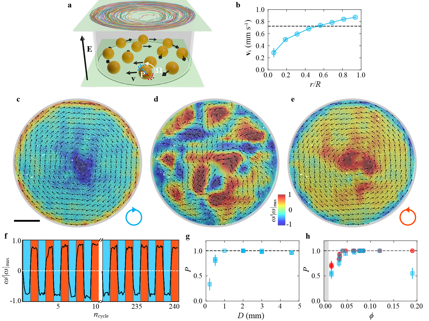
Figure 1: Vortex chiral state reversal induced by a temporal modulation of activity. a, A sketch of the experimental setup. Red and blue specks illustrate induced positive and negative charges around a particle. Particles develop a tilted dipole $\bf{P}$ and rotate with an angular velocity $\bf{\Omega}$ resulting in a translational velocity $\bf{v}$ along the surface. Particle trajectories in a typical self-organized vortex of rollers are illustrated as an insert on the top cell surface. The local particle density in the vortex is not uniform with a noticeable depletion in the center of the well. b, Averaged tangential velocities $v_{\text{t}}$ of particles in the roller vortex as a function of the distance from the center. $R$ is the radius of the well. The dash line shows the averaged velocity $v_{0}$ of an isolated roller measured in a dilute sample under the same experimental conditions. The error bars are standard deviations of the mean. c-e, Snapshots of superimposed velocity (arrows) and vorticity (background color) fields of the rollers during a vortex reversal under a temporal modulation of the activity. c, A stable initial roller vortex with a clockwise rotation. d, Intermittent flocking after re-activation of the system. Rollers initially move mostly towards the center of the cell. e, A stable vortex with a counter-clockwise rotation evolved from the state shown in d. The blue and red circles with an arrow illustrate the chirality of the states. The scale bar is 0.2 mm. The field strength $E=$ 2.7 V $\text{\,}\mathrm{\SIUnitSymbolMicro m}$^-1, the particle area fraction $\phi=0.12$. See Supplementary Video 1. f, Cycling of the vortex chiral state by a temporal termination and subsequent restoration of the electric field. The black curve shows normalized magnitude of the vorticity in the vortex center. Blue spans indicate CW vortices, and red spans correspond to CCW vortices. The vortex reversal is observed for every one of 240 cycles. The particle area fraction $\phi=$ 0.08. See Supplementary Video 1 for details. g, The reversal probability $P$ as a function of the well diameter $D$. The particle area fraction $\phi$ = 0.07$\pm$0.01. $P=N_{\text{r}}/N_{\text{t}}$, where $N_{\text{r}}$ is the number of times the vortex reversal is observed during $N_{\text{t}}$ activity cycles. h, The reversal probability $P$ (blue squares) as a function of the particles area fraction $\phi$ for $D=$ 2 mm. Red circles illustrate the probability of the vortex formation in the same system. A shaded area indicates the area fractions $\phi<$ 0.01 where no stable vortex is observed. Dash lines depict $P=1$. Error bars are standard deviations of the mean.

The roller vortex is robust and remains stable as long as the system is energized. Typical velocity and vorticity fields in a stable vortex are shown in Fig. 1c. Two possible chiral states of the vortex, clockwise (CW) or counter-clockwise (CCW), are equally probable, and the system spontaneously selects one in the course of the vortex self-assembly from initially random distribution of particles. When the electric field is switched off, particles come to rest within a time scale given by the Maxwell-Wagner relaxation time $\tau_{\text{MW}}$ and viscous time scale $\tau_{\nu}$ that are both of the order of 1 ms for our system. The particle arrangements appear to be random and the direction of the original vortex cannot be easily identified. A cessation of the activity beyond $\tau_{\text{MW}}=(\epsilon_{\text{p}}+2\epsilon_{\text{f}})/(\sigma_{\text{p}}+2\sigma_{\text{f}})$, where $\epsilon_{\text{p,f}}$ and $\sigma_{\text{p,f}}$ are respective particle and fluid permittivities and conductivities, preserves the particle positions but erases their previous velocities, polarizations and resets aligning forces. Once the system is re-energized by the same DC electric field, particles initially move mostly toward the center of the well where the density is the lowest (see Fig. 1d). Eventually the rollers redistribute over the well and form a single vortex with the direction of rotation opposite to the state preceding the cessation of the activity (Fig. 1e, see also Supplementary Video 1).

The probability of the vortex reversal, $P$, achieves 1 in a wide range of explored experimental parameters (see Fig. 1f-h). The activity cessation time $\tau_{\text{off}}$ in a range from 10 ms up to 5 minutes has been probed and resulted in no significant effect on the reversal probability upon the re-energizing the system. This observation allows us to exclude the effects caused by remnant hydrodynamic flows or polarization. When $\tau_{\text{off}}$ is comparable to $\tau_{\text{MW}}$ and $\tau_{\nu}$, the vortex does not terminate completely and its subsequent reversal is not triggered. Persistence of the rotation at small $\tau_{\text{off}}$ is supported by the incomplete depolarization of the particles and the inertia of a macroscopic hydrodynamic flow.

The robustness of the chiral state reversal suggests the presence of a dynamic state memory in the ensemble. The information that is preserved long after the termination of activity, can be stored only in the particle positional arrangements of the ensemble.

The reversal probability depends on the system diameter, $D$, and particle area fraction $\phi$ (see Fig. 1g, h). For small diameters the persistence length of roller trajectories is reduced by the high curvature of the walls and the vortex formation probability decreases. The chiral state reversal is robust in a wide range of the particle number densities ($0.04<\phi<0.12$). For dilute area fractions ($\phi<0.03$), the inter-particle interactions are weak and motion of the rollers is uncorrelated. At higher area fractions ($\phi>0.19$), while the vortex formation probability is high, the reversal probability decreases. The repulsions between the particles at high particle number density reduce the degree of density variations in the system, leading to a decrease in the “quality” of the stored information in asymmetric particle arrangements against the background noise.

Figure 2: Rollers dynamics during chirality reversal of the polar state. a-f, Snapshots of a roller vortex undergoing the chiral state reversal. The electric field is reapplied at $t=$ 0 s after a short cessation of activity, $\tau_{\text{off}}$= 0.5 s. Rollers are shown as circles colored according to the magnitude of the tangential velocity $\bf{v}_{\text{t}}$. a, Particles in a stable CCW vortex. b, Particles are at rest when the electric field is off. c, Rollers ensemble moments after the system is re-energized. d, Most of the particles move towards the center of the well. CW (blue) and CCW (red) roller flocks are formed. e, Particles redistribute over the well. The CW rotating flocks start to dominate over those with CCW rotation. f, A stable CW vortex is formed. The scale bar is 0.2 mm. See also Supplementary Video 2. g, Time evolution of the average normal (blue) and tangential (red) velocities during the chiral state reversal. h, Same process as in g is calculated in simulations (see Methods and Supplementary Note 1). Gray areas indicate the state with the electric filed off.

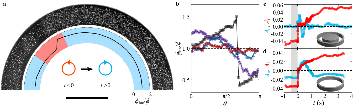
Figure 3: Positional order asymmetries in polar active fluids. a, Microscopic image illustrates the spatial distribution of rollers in a circular track (only half of the track is shown) with a width $W=$ 0.25 mm. Particles move CCW and form a stable traveling band along the track. The black curve in the inner ring illustrate the average azimuthal particle density. The background color of the inner ring indicates the direction of initial rollers velocities at the moment when the DC electric field is re-applied. The scale bar is 0.5 mm. See also Supplementary Video 3. b, Azimuthal density distribution of rollers in circular tracks with outer diameter $D=2$ mm and the width $W=$ 0.25 mm (black), 0.50 mm (purple), 0.75 mm $\text{\,}\mathrm{(}$blue) and in the well (red) as a function of azimuthal angle. Average particles area fraction $\phi=0.12$. A half of the track (or well) is shown. c-d, Evolutions of local order parameters $A_{\text{n}}$ (blue) and $A_{\text{t}}$ (red) in a track of the width $W=$ 0.25 mm (c) and a well with $D=$ 2 mm (d) during a vortex reversal. The initial direction of the vortex is CCW. The area fraction $\phi=$ 0.12. Oscillations of $A_{\text{n}}$ at the initial stage of the band formation in a track correspond to the reflections of density bands from the walls. A non-zero value of $A_{\text{n}}$ reflects the existence of a particle density gradient along the normal direction in the well. Shaded areas indicate field-off time.

While the observed chiral state reversal is a remarkably robust phenomenon, the formation of a new polar state upon re-activation proceeds through a seemingly chaotic process (see Supplementary Video 2). In a stable vortex illustrated in Fig. 2a, all particles initially move CCW with an average tangential velocity of $\textbf{v}_{\text{t}}$ = 0.82 mm s^-1 and nearly zero normal velocity. When the DC electric field is switched off, all particles cease to roll without significant alteration of their relative positions set during the vortex rotation (Fig. 2b). After the field is restored, the particles restart motion in seemingly random directions (Fig. 2c). Flocks of rollers with spatially correlated velocities form (Fig. 2d,e ). The center of the well becomes the densest part of the system in a fraction of a second, and within the next few seconds, particles redistribute into a new stable vortex with a depletion zone in the center (Fig. 2f). The process is characterized by the behavior of the average tangential and normal components of the rollers velocities shown in Fig. 2g. At the very first moments upon reactivation, the tangential motion of particles is mostly chaotic, manifested by the emergence of small flocks of rollers moving in both CW and CCW directions. In contrast, the normal component of the average roller velocities sharply increases at re-activation and eventually subside to zero. While initial fractions of particles moving CCW and CW are approximately the same, the CW fraction steadily grows with time and eventually plateaus with the average tangential velocity reaching $\textbf{v}_{\text{t}}=-0.82$ mm s^-1 (equal in magnitude but opposite in the direction to the initial vortex).

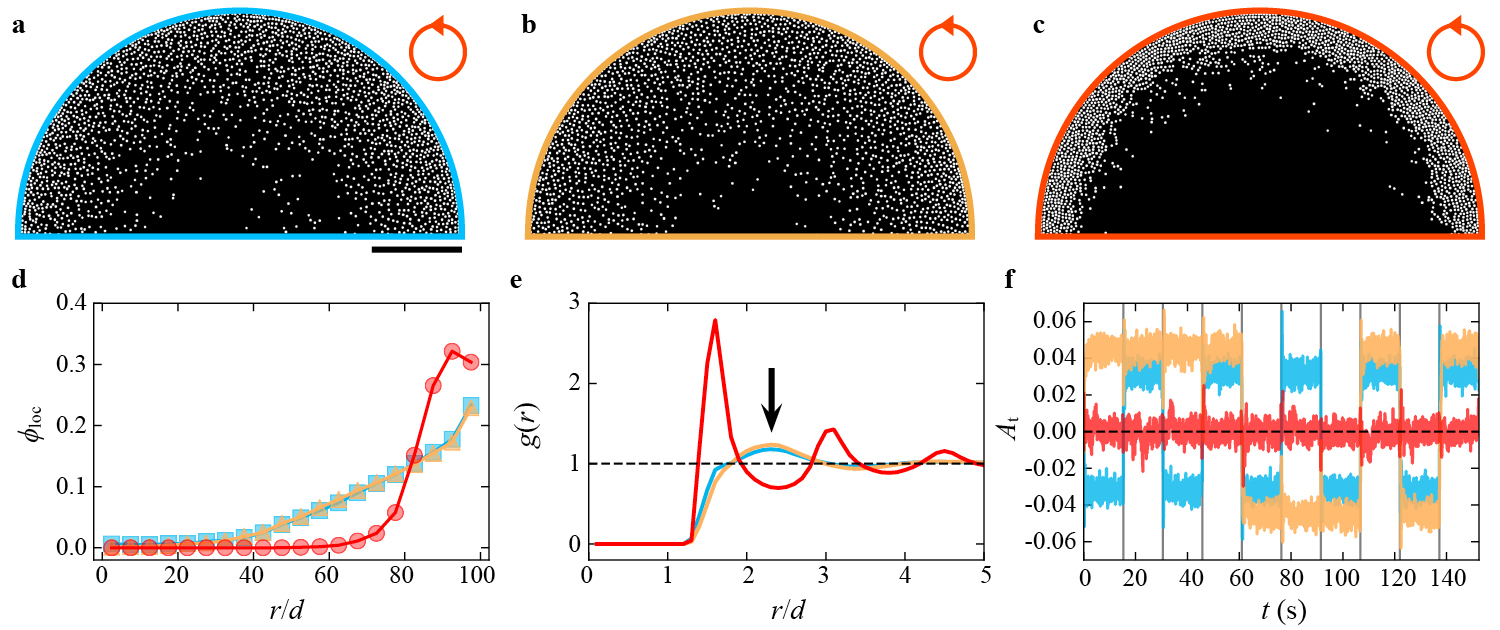
Figure 4: Role of microscopic interactions in the chiral state reversal. a-c, Simulation snapshots of stable spontaneous vortices formed under three different scenarios. a, Both electrostatic and hydrodynamic interactions between rollers are included in the model. b, only hydrodynamic interactions drive rollers dynamics. c, only electrostatic interactions contribute to the collective dynamics. Only half of the wells are shown. The scale bar is 0.2 mm. The particle area fraction $\phi$ = 0.10 and the field strength is $E=$ 2.0 V $\text{\,}\mathrm{\SIUnitSymbolMicro m}$^-1. d, Radial variations of local particle density, $\phi_{\text{loc}}$, in a stable vortex formed with both electrostatic and hydrodynamic interactions (blue), only hydrodynamic (orange), and only electrostatic (red) interactions. $r$ is the distance of particles from the center of the well. e, Positional pair correlation functions $g(\text{r})$ of particles in stable vortices shown in a-c. The same color coding is used as in d. The black arrow in e points to the identical location of a first peak for scenarios a and b. f, Local order parameter $A_{\text{t}}$ calculated for 10 activity cessation cycles. The ensemble does not store any information in the positional order when only electrostatic interactions govern collective dynamics of the rollers (red curve). Local positional order asymmetries encoding the information about the chiral state of the ensemble develop only for scenarios including hydrodynamic interactions (blue, orange). Nevertheless, robust reversal is observed only when both hydrodynamic and electrostatic interactions are present(blue).

The chirality of the collective motion can be similarly reversed in an annulus (see Supplementary Video 3). However, in contrast to the cylindrical confinement, particle traveling bands with a visible local density gradient along the direction of motion are observed in these experiments. The traveling density bands carry the information about the chirality of the polar state. Upon activity termination, it is possible to recover the previous direction of the band motion by a snapshot of the track. In a stable CCW-rotating band shown in Fig. 3a, the local particle density $\phi_{\text{loc}}$ increases slowly with an azimuth angle toward the front of the band, and then abruptly drops at the frontier. When the system is re-energized, the inter-particle repulsive interactions push rollers away from the high-density regions resulting in a reversal of the band motion.

As the width of the track grows, the tangential density gradient (i.e., the band structure) dissolves and completely vanishes in the case of a well (Fig. 3b). Nevertheless, the reversal of the vortex chiral state upon temporal modulation of activity is preserved. It suggests that a structural asymmetry encoded in the local particle positions is now hidden by being redistributed over the whole ensemble. To unveil intrinsic asymmetries in the positional arrangements of rollers in a vortex, we introduce two local order parameters $A_{\text{n}}$ and $A_{\text{t}}$.

$$A_{\text{n,t}}=\langle\mathbf{F}_{i}\cdot\mathbf{u}^{i}_{\text{n,t}}\rangle_{i}.$$ (1)

Here, $\mathbf{F}_{i}$ is a model repulsive unit force acting on the particle $i$ from the the nearest neighbors (See Supplementary Note 2), and $\mathbf{u}^{i}_{\text{n,t}}$ are normal and tangential unit vectors respectively at the position of the particle $i$. $\langle...\rangle_{i}$ indicates averaging over all particles. We can simplify the averaging over the neighbors by taking into account only a single nearest particle in Eq. 1.

Equipped with two order parameters we analyze the reversal process in a circular track and a well. The non-zero value of $A_{\text{t}}$ in the track during a stable collective motion indicates the density gradient along the tangential direction, see Fig. 3c. Simultaneously, $A_{\text{n}}$ is zero within the noise level during the band motion, indicating the absence of normal particle density gradients in a track. Both $A_{\text{n}}$ and $A_{\text{t}}$ remain nearly constant while the system is in a stable dynamic state. The positive (or negative) value of $A_{\text{t}}$ indicates a CW (or CCW) vortex or band. In a well, the value of $A_{\text{t}}$ also exhibits stable non-zero values comparable in magnitude to those observed in narrow tracks, even though the density bands are absent (Fig. 3d).

To elucidate the physics underlying the chiral state memory formation in the ensemble of active rollers and uncover mechanisms leading to the encoding and subsequent retrieval of the information by the active system we develop a particle-based model by coupling the Quincke rotation mechanism[25] with Stokesian Dynamics[27] (see Methods and Supplementary Note 1). The simulations correctly capture all phenomenology observed in the roller ensemble upon temporal modulation of the activity (Fig. 2h, Supplementary Figure 1 and Supplementary Video 4, 5).

In ensembles of Quincke rollers both electrostatic and hydrodynamic interactions contribute to the velocity alignment processes resulting in a coherent large-scale motion [13]. To identify the microscopic mechanisms driving the emergence of a dynamic state memory encoded in the particles positional arrangements, we investigate the behavior of the system when either electrostatic or hydrodynamic interactions are “turned off” in the simulations. Without electrostatic interactions, a stable vortex still forms and has a structure similar to a regular vortex with both types of interactions present (see Fig. 4a,b and Supplementary Video 4). The absence of the electrostatic interactions does not affect significantly the overall particle distribution in the vortex as indicated by a radial particle density distribution (Fig. 4d) and pair correlation function, $g(r)$ (Fig. 4e). The vortex also preserves the non-zero local order parameter $A_{\text{t}}$ indicating the presence of the local positional order asymmetries (Fig. 4f).

In contrast, the absence of the long-range hydrodynamic interactions results in particle accumulation near the boundary of the well (Fig. 4c-d). The vortex forms, however, with most of the particles densely packed near the boundary as indicated by multiple peaks of $g(r)$ (see Fig. 4e). Importantly, the order parameter $A_{\text{t}}$ is at the noise level, see Fig. 4f, indicative that the local asymmetries along the tangential direction disappear. The plots of the order parameter $A_{\text{t}}$ as the system undergoes activity-inactivity cycles demonstrate that in both cases of truncated interactions no robust vortex reversal is observed, and the probability of the reversal is close to 0.5 suggestive that each time the system randomly selects the chiral state. It implies very specific roles of those two interactions. The hydrodynamic interactions are responsible for the development of asymmetries in the local positional order within the vortex that effectively encode the information about the chiral state. Electrostatic interactions on the other hand are crucial for de-coding this information in the process of vortex formation. When both ingredients are present the system exhibits remarkable reversibility of its chiral state upon temporal control of the activity by the external field.

To further generalize the results we have constructed a phenomenological model with a bare minimum of “ingredients”: isotropic short-range repulsions between particles and velocity alignment interactions (see Supplementary Note 3). The model mimics main experimental observations and captures chiral state reversal upon re-energizing of the ensemble with information encoded exclusively in the particle positional order (Supplementary Video 6). It suggests that in general, the presence of short-range isotropic repulsions and velocity alignment interactions is enough to develop the local density asymmetries forming the basis for the ensemble polar state memory.

In this study, we demonstrate that active liquids formed by motile particles are capable of developing memory of their dynamic states and store it in seemingly random positional arrangements of the particles. We show that an ensemble of Quincke rollers stores the information about the globally correlated state via local inter-particle positional arrangements. The information is preserved long after a complete cessation of activity beyond the Maxwell-Wagner and viscous times. Surprisingly, a relatively weak level of the local arrangement asymmetry is enough to prescribe the direction of the global vortex motion with high fidelity.

We isolate the role of hydrodynamics as a driving force in the development of the ensemble chiral state memory, and reveal the crucial role of electrostatic repulsive interactions as a main mechanism for the system to access the stored information. The dynamics of the global chiral state reversal involves seemingly chaotic evolution of multiple flocks indicative that the information readout in the system is not instantaneous and relies on multiple inter-particle interactions. However, the reversal process is robust, and a temporal control of the activity can be exploited to systematically command the subsequent polar states of an active liquid. We envision that with the chirality of the emergent states controlled on-demand, active liquids offer new possibilities for a flow manipulation, transport, and mixing at the microscale.

Competing interests

The authors declare no competing interests.

Methods

Experimental setup

Polystyrene colloidal particles (G0500, Thermo Scientific) with an average diameter $d$ of 4.8 $\text{\,}\mathrm{\SIUnitSymbolMicro m}$ are dispersed in a 0.15 mol L^-1 dioctyl sulfosuccinate sodium (AOT)/hexadecane solution. The colloidal suspension is then injected into a cylindrical chamber made out of a SU-8 cylindrical spacer confined between two parallel ITO-coated glass slides (IT100, Nanocs). A typical height, L, and inner diameter of the experimental cell, D, are 45 $\text{\,}\mathrm{\SIUnitSymbolMicro m}$ and 1 mm, respectively. A uniform DC electric field is introduced by applying a voltage between two ITO-coated glass slides. The field strength $E$ is kept at 2.7 V $\text{\,}\mathrm{\SIUnitSymbolMicro m}$^-1. The period of the pulse function of the DC field is $T=$ 10 s for $\phi<0.1$ and 20 s for $\phi>0.1$ with the zero-voltage time interval of $0.5$ s and $1$ s respectively.

Viscous time scale $\tau_{\nu}\sim L^{2}/\nu$. Here , $\nu$ is kinematic viscosity of the media. $\tau_{\nu}\simeq$ 1 ms.

Dynamics of the colloidal suspensions is captures by an Olympus IX71 inverted microscope (4$\times$ objective) and a fast-speed camera (IL 5, Fastec Imaging). To optimize the image processing the frame rates are selected at 120 FPS for particle image velocimetry (PIV) and 850-1000 FPS for particle tracking velocimetry (PTV). PIV, PTV and further data analysis are carried out with a custom-made scripts in Matlab, Python, and Trackpy.

Measurements of the local area fraction

The local area fractions $\phi_{\text{loc}}$ in Fig. 3a-b is measured by dividing the track into sectors with 52.4 $\text{\,}\mathrm{\SIUnitSymbolMicro m}$ outside arc length. $\phi_{\text{loc}}$ is the particle area fraction in each sector. In Fig. 4d, the well is divided into concentric rings with 25 $\text{\,}\mathrm{\SIUnitSymbolMicro m}$ thickness, and the area fraction is calculated for each ring.

Numerical model

We developed a particle-based simulation of a population of Quincke rollers by combining the Quincke rotation mechanism[25], which enables the active motion of particles, together with Stokesian Dynamics[27] to account for the many-particles hydrodynamic interactions. In this work, the simulation models $N=4096$ spherical particles of radius $a=2.5$ $\text{\,}\mathrm{\SIUnitSymbolMicro m}$ with dielectric permittivity $\epsilon_{\text{p}}=3$ and conductivity $\sigma_{\text{p}}=0$ immersed in a weakly conducting liquid (AOT/hexadecane) with dielectric permittivity $\epsilon_{\text{l}}=2$ and conductivity $\sigma_{\text{l}}=2\times 10^{-8}$ S m^-1. The viscosity of the fluid is $\eta=2\ \mathrm{mPa\cdot s}$. A uniform external electric field $\mathbf{E}_{0}=E_{0}\mathbf{\hat{z}}$ ($E_{0}$ = 2 V $\text{\,}\mathrm{\SIUnitSymbolMicro m}$^-1) is applied along the z-axis. The particles are confined inside a circular well of diameter $D=1\ \mathrm{mm}$, which corresponds to an area fraction of 10 %. Because the particles are strongly attracted to the bottom electrode surface, for simplicity, the motion of the particles is constrained at the 2D plane $h$ = 0.1$a$ above the bottom electrode.
To leading order of approximation[28, 29], each particle carries an electric dipole moment resulting from the dominant dipolar interfacial charge at each particle-fluid interface and evolves according to the surface charge conservation equation:

$$\frac{\mathrm{d}\mathbf{P}^{\alpha}}{\mathrm{d}t}=\mathbf{\Omega}^{\alpha}\times\left(\mathbf{P}^{\alpha}-\chi^{\infty}\mathbf{E}^{\alpha}\right)-\frac{1}{\tau}\left(\mathbf{P}^{\alpha}-\chi^{0}\mathbf{E}^{\alpha}\right)$$ (2)

where $\mathbf{P}^{\alpha}$ and $\mathbf{\Omega}^{\alpha}$ are the electric dipole moment and the angular velocity of the $\alpha$-th particle, $\mathbf{E}^{\alpha}=\mathbf{E}_{0}+\delta\mathbf{E}^{\alpha}$ is the electric field at $\alpha$-th particle’s location and $\delta\mathbf{E}^{\alpha}$ includes contributions from both the surrounding particles and their image dipoles; $\chi^{\infty}=4\pi\epsilon_{0}a^{3}\frac{\epsilon_{\text{p}}-\epsilon_{\text{l}}}{\epsilon_{\text{p}}+2\epsilon_{\text{l}}}$ and $\chi^{0}=4\pi\epsilon_{0}a^{3}\frac{\sigma_{\text{p}}-\sigma_{\text{l}}}{\sigma_{\text{p}}+2\sigma_{\text{l}}}$ are the respective high-frequency and low-frequency polarizability; $\tau=\frac{\epsilon_{\text{p}}+2\epsilon_{\text{l}}}{\sigma_{\text{p}}+2\sigma_{\text{l}}}$ is the Maxwell-Wagner relaxation time[30]. Please be noted that eqn. 2 does not depend on the fluid flow velocity, which essentially ignores possible electro-osmotic flow effects on the dynamics of surface charge transport.
Each Quincke particle interacts with the external electric fields:

$$\mathbf{T}^{\alpha}_{\text{ext}}=\mathbf{P}^{\alpha}\times\mathbf{E}_{0}$$ (3)

and also with its surrounding rollers via the screened dipole-dipole interaction and Coulombic interaction:

$$U^{\alpha\beta}_{\text{d}}(\mathbf{r})=\varepsilon_{\text{d}}\exp{\left(-\kappa_{\text{d}}r\right)}\left[\frac{1}{r^{3}}\left(\mathbf{P}^{\alpha}\cdot\mathbf{P}^{\beta}\right)-\frac{3}{r^{5}}\left(\mathbf{P}^{\alpha}\cdot\mathbf{r}\right)\left(\mathbf{P}^{\beta}\cdot\mathbf{r}\right)\right]$$ (4)

$$U^{\alpha\beta}_{\text{q}}(r)=\varepsilon_{\text{q}}\frac{\exp{\left(-\kappa_{\text{q}}r\right)}}{r}$$ (5)

where $\mathbf{r}=\mathbf{r}^{\alpha}-\mathbf{r}^{\beta}$, $r=\left|\mathbf{r}\right|$ and $\mathbf{r}^{\alpha}$ is the position of $\alpha$-th particle; $\varepsilon_{\text{q}}$ and $\kappa_{\text{q}}^{-1}$ are the interaction strength and the screening length of the Coulombic interaction, which is included to account for steric interactions and possible net charges on each particles. Since the concentration of AOT is 0.15 mol L^-1, the $\kappa_{\text{q}}^{-1}$ is estimated[31] as $0.2a$ $(500\ \mathrm{nm})$, which makes the Coulombic interaction highly short-ranged and $\epsilon_{\text{q}}$ is adjusted to ensure particles do not overlap during simulations. The interaction strength and the screening length of the dipole-dipole interaction are $\varepsilon_{\text{d}}$ and $\kappa_{\text{d}}^{-1}$, respectively; $\epsilon_{\text{d}}=1.0$ and $\kappa_{\text{d}}^{-1}\approx 5a\gg\kappa_{\text{q}}^{-1}$ to ensure that each particle can interact with its neighbors about one particle diameter away.
The total force $\mathbf{F}^{\alpha}$ and the total torque $\mathbf{T}^{\alpha}$ acting on each particles can be obtained by summing over all microscopic interactions. Then, the corresponding motion of each particles are calculated via the mobility matrix formulation based on the configuration of N particles[32]:

$$\begin{pmatrix}\mathbf{U}\\ \mathbf{\Omega}\end{pmatrix}=\mathcal{M}\begin{pmatrix}\mathbf{F}\\ \mathbf{T}\end{pmatrix}$$ (6)

where $\mathbf{U}=\{\mathbf{U}^{1},\cdots,\mathbf{U}^{N}\}$ and $\mathbf{\Omega}=\{\mathbf{\Omega}^{1},\cdots,\mathbf{\Omega}^{N}\}$ are the translational and angular velocity vector of N particles, respectively; $\mathbf{F}=\{\mathbf{F}^{1},\cdots,\mathbf{F}^{N}\}$ and $\mathbf{T}=\{\mathbf{T}^{1},\cdots,\mathbf{T}^{N}\}$ are the force and torque vector of N particles, respectively; $\mathcal{M}(\mathbf{r}^{1},\cdots,\mathbf{r}^{N})$ is the grand mobility tensor, which maps the applied forces and torques into the respective translational and angular velocities of each particles.
The explicit expressions of the mobility tensor in an unbound medium have been derived via the multipole expansion method for well-separated pair of particles[33, 32] or using the Rotne-Prager-Yamakwa (RPY) approximation for overlapping particles[34, 35]. Furthermore, additional wall corrections of these mobility tensors have also been derived for the case near an infinite no-slip boundary based on the method of reflection[36, 37]. In this work, the hydrodynamic interactions between Quincke rollers are modelled with the Rotne-Prager-Blake tensor with wall corrections[19, 38].
Besides the deterministic motions calculated via eqn. 6, the stochastic Brownian noise should also be included to account for the thermal fluctuations. In principle, the hydrodynamically-correlated Brownian noise which obeys the fluctuation-dissipation theorem[39] should be used, i.e., $\mbox{\boldmath$\xi$}=\sqrt{2k_{B}T}\mathcal{M}^{1/2}\mathcal{W}+k_{B}T\mbox{\boldmath$\nabla$}\cdot\mathcal{M}$, where $k_{B}$ is the Boltzmann constant, $T$ is the temperature, $\mathcal{W}$ is a vector of independent standard Gaussian noise. However, for a typical Quincke roller system, the active velocity ($\sim$ 1 mm s^-1) driven by external electric fields is much large than the diffusive velocity ($\sim$ 0.1 $\text{\,}\mathrm{\SIUnitSymbolMicro m}$ s^-1) caused by the thermal energy. The Brownian noise is only important when the roller just starts moving and is negligible once the roller picks up speed. For simplicity, the uncorrelated Brownian noise is used instead:

$$\mbox{\boldmath$\xi$}\approx\sqrt{2k_{B}\chi T}\mathcal{M}^{1/2}_{bulk}\mathcal{W}$$ (7)

where $\mathcal{M}_{bulk}$ is the diagonal grand mobility tensor in an unbound medium and $\chi\approx 0.1$ is a factor which accounts for the diffusion hindrance near the boundary[40].
Adding the deterministic hydrodynamic velocities (eqn. 6) and the stochastic Brownian velocities (eqn. 7) together, the system evolves according to the following equation of motion:

$$\frac{\mathrm{d}}{\mathrm{d}t}\begin{pmatrix}\mathbf{r}\\ \mathbf{q}\end{pmatrix}=\mathcal{M}\begin{pmatrix}\mathbf{F}\\ \mathbf{T}\end{pmatrix}+\mbox{\boldmath$\xi$}$$ (8)

where $\mathbf{r}=\{\mathbf{r}^{1},\cdots,\mathbf{r}^{N}\}$ and $\mathbf{q}=\{\mathbf{q}^{1},\cdots,\mathbf{q}^{N}\}$ are the position and orientation vector of N particles, respectively. Solving the above equation of motion (eqn. 8) simultaneously with the time evolution equation of the electric dipole moment (eqn.2) enables the dynamic simulations of a population of Quincke rollers.

References

- [1] Vicsek, T. & Zafeiris, A. Collective motion. Physics Reports 517, 71–140 (2012).
- [2] Marchetti, M. C. et al. Hydrodynamics of soft active matter. Reviews of Modern Physics 85, 1143 (2013).
- [3] Aranson, I. S. Active colloids. Physics-Uspekhi 56, 79 (2013).
- [4] Snezhko, A. Complex collective dynamics of active torque-driven colloids at interfaces. Current Opinion in Colloid & Interface Science 21, 65–75 (2016).
- [5] Zöttl, A. & Stark, H. Hydrodynamics determines collective motion and phase behavior of active colloids in quasi-two-dimensional confinement. Physical review letters 112, 118101 (2014).
- [6] Wu, K.-T. et al. Transition from turbulent to coherent flows in confined three-dimensional active fluids. Science 355, eaal1979 (2017).
- [7] Bricard, A. et al. Emergent vortices in populations of colloidal rollers. Nature communications 6, 7470 (2015).
- [8] Kaiser, A., Snezhko, A. & Aranson, I. S. Flocking ferromagnetic colloids. Science advances 3, e1601469 (2017).
- [9] Peruani, F. et al. Collective motion and nonequilibrium cluster formation in colonies of gliding bacteria. Physical review letters 108, 098102 (2012).
- [10] Schaller, V., Weber, C., Semmrich, C., Frey, E. & Bausch, A. R. Polar patterns of driven filaments. Nature 467, 73 (2010).
- [11] Sumino, Y. et al. Large-scale vortex lattice emerging from collectively moving microtubules. Nature 483, 448 (2012).
- [12] Sokolov, A. & Aranson, I. S. Physical properties of collective motion in suspensions of bacteria. Physical review letters 109, 248109 (2012).
- [13] Bricard, A., Caussin, J.-B., Desreumaux, N., Dauchot, O. & Bartolo, D. Emergence of macroscopic directed motion in populations of motile colloids. Nature 503, 95 (2013).
- [14] Yan, J. et al. Reconfiguring active particles by electrostatic imbalance. Nature materials 15, 1095 (2016).
- [15] Kokot, G. et al. Active turbulence in a gas of self-assembled spinners. Proceedings of the National Academy of Sciences 114, 12870–12875 (2017).
- [16] Doostmohammadi, A., Ignés-Mullol, J., Yeomans, J. M. & Sagués, F. Active nematics. Nature communications 9, 1–13 (2018).
- [17] Zhang, B., Sokolov, A. & Snezhko, A. Reconfigurable emergent patterns in active chiral fluids. Nature Communications 11, 1–9 (2020).
- [18] Martin, J. E. & Snezhko, A. Driving self-assembly and emergent dynamics in colloidal suspensions by time-dependent magnetic fields. Reports on Progress in Physics 76, 126601 (2013).
- [19] Driscoll, M. et al. Unstable fronts and motile structures formed by microrollers. Nature Physics 13, 375 (2017).
- [20] Weber, C. A. et al. Long-range ordering of vibrated polar disks. Physical review letters 110, 208001 (2013).
- [21] Kokot, G. & Snezhko, A. Manipulation of emergent vortices in swarms of magnetic rollers. Nature communications 9, 2344 (2018).
- [22] Massana-Cid, H., Codina, J., Pagonabarraga, I. & Tierno, P. Active apolar doping determines routes to colloidal clusters and gels. Proceedings of the National Academy of Sciences 115, 10618–10623 (2018).
- [23] Han, K. et al. Reconfigurable structure and tunable transport in synchronized active spinner materials. Science advances 6, eaaz8535 (2020).
- [24] Palacci, J., Sacanna, S., Steinberg, A. P., Pine, D. J. & Chaikin, P. M. Living crystals of light-activated colloidal surfers. Science 339, 936–940 (2013).
- [25] Quincke, G. Ueber rotationen im constanten electrischen felde. Annalen der Physik 295, 417–486 (1896).
- [26] Melcher, J. & Taylor, G. Electrohydrodynamics: a review of the role of interfacial shear stresses. Annual review of fluid mechanics 1, 111–146 (1969).
- [27] Durlofsky, L., Brady, J. F. & Bossis, G. Dynamic simulation of hydrodynamically interacting particles. Journal of Fluid Mechanics 180, 21–49 (1987).
- [28] Das, D. & Saintillan, D. Electrohydrodynamic interaction of spherical particles under quincke rotation. Phys. Rev. E 87, 043014 (2013).
- [29] Pannacci, N., Lobry, L. & Lemaire, E. How insulating particles increase the conductivity of a suspension. Phys. Rev. Lett. 99, 094503 (2007).
- [30] Jones, T. B. & Jones, T. B. Electromechanics of Particles (Cambridge University Press, 2005).
- [31] Sainis, S. K., Germain, V., Mejean, C. O. & Dufresne, E. R. Electrostatic interactions of colloidal particles in nonpolar solvents: Role of surface chemistry and charge control agents. Langmuir 24, 1160–1164 (2008).
- [32] Sangtae Kim, S. J. K. Microhydrodynamics - Principles and Selected Applications (Dover Publications, Inc., 2005).
- [33] Brady, J. F. & Bossis, G. Stokesian dynamics. Annual Review of Fluid Mechanics 20, 111–157 (1988).
- [34] Rotne, J. & Prager, S. Variational treatment of hydrodynamic interaction in polymers. J. Chem. Phys. 50, 4831–4837 (1969).
- [35] Wajnryb, E., Mizerski, K. A., Zuk, P. J. & Szymczak, P. Generalization of the rotne-prager-yamakawa mobility and shear disturbance tensors. Journal of Fluid Mechanics 731, R3 (2013).
- [36] Blake, J. R. A note on the image system for a stokeslet in a no-slip boundary. Mathematical Proceedings of the Cambridge Philosophical Society 70, 303–310 (1971).
- [37] Swan, J. W. & Brady, J. F. Simulation of hydrodynamically interacting particles near a no-slip boundary. Physics of Fluids 19, 113306 (2007).
- [38] Balboa Usabiaga, F., Delmotte, B. & Donev, A. Brownian dynamics of confined suspensions of active microrollers. J. Chem. Phys. 146, 134104 (2017).
- [39] Ermak, D. L. & McCammon, J. A. Brownian dynamics with hydrodynamic interactions. J. Chem. Phys. 69, 1352–1360 (1978).
- [40] Kazoe, Y. & Yoda, M. Measurements of the near-wall hindered diffusion of colloidal particles in the presence of an electric field. Appl. Phys. Lett. 99, 124104 (2021).
Acknowledgements
The research of B. Z., A. Sok., A. S. at Argonne National Laboratory was supported by the U.S. Department of Energy, Office of Science, Basic Energy Sciences, Materials Sciences and Engineering Division. Use of the Center for Nanoscale Materials, an Office of Science user facility, was supported by the U.S. Department of Energy, Office of Science, Office of Basic Energy Sciences, under Contract No. DE-AC02-06CH11357. H.Y. and M.O.d.l.C. were supported by the Center for Bio-Inspired Energy Science, an Energy Frontier Research Center funded by the US Department of Energy, Office of Science, Basic Energy Sciences under Award DE-SC0000989.