DISTRIBUTED STOCHASTIC OPTIMIZATION WITH LARGE DELAYS

Abstract.

One of the most widely used methods for solving large-scale stochastic optimization problems is distributed asynchronous stochastic gradient descent (DASGD), a family of algorithms that result from parallelizing stochastic gradient descent on distributed computing architectures (possibly) asychronously. However, a key obstacle in the efficient implementation of DASGD is the issue of delays: when a computing node contributes a gradient update, the global model parameter may have already been updated by other nodes several times over, thereby rendering this gradient information stale. These delays can quickly add up if the computational throughput of a node is saturated, so the convergence of DASGD may be compromised in the presence of large delays. Our first contribution is that, by carefully tuning the algorithm’s step-size, convergence to the critical set is still achieved in mean square, even if the delays grow unbounded at a polynomial rate. We also establish finer results in a broad class of structured optimization problems (called variationally coherent), where we show that DASGD converges to a global optimum with probability $1$ under the same delay assumptions. Together, these results contribute to the broad landscape of large-scale non-convex stochastic optimization by offering state-of-the-art theoretical guarantees and providing insights for algorithm design.

1. Introduction

With the advent of high-performance computing infrastructures that are capable of handling massive amounts of data, distributed stochastic optimization has become the predominant paradigm in a broad range of applications in operations research [15, 16, 30, 50, 45, 44, 32]. Starting with a series of seminal contributions by Tsitsiklis et al. [49], recent years have witnessed a commensurate surge of interest in the parallelization of first-order methods, ranging from ordinary (stochastic) gradient descent [1, 42, 40, 11, 31, 18, 35], to coordinate/dual coordinate descent [34, 2, 33, 46, 17, 47], randomized Kaczmarz algorithms [34], online methods [41, 26, 22, 24], block coordinate descent [51, 36, 52], ADMM [53, 23], and many others.

This popularity is a direct consequence of Moore’s law of silicon integration and the commensurately increased distribution of computing power. For instance, in a typical supercomputer cluster, up to several thousands of “workers” (or sometimes tens of thousands) perform independent computations with little to no synchronization – as the cost of such coordination quickly becomes prohibitive in terms of overhead and energy spillage. Similarly, massively parallel computing grids and data centers (such as those of Google, Amazon, IBM or Microsoft) may house up to several million computing nodes and/or servers, all working asynchronously to execute a variety of different tasks. Finally, taking the concept of distributed computing to its logical extreme, volunteer computing grids (such as Berkeley’s BOINC infrastructure or Stanford’s folding@home project) essentially span the entire globe and harness the computing power of a vast, heterogeneous network of non-clustered nodes that receive and process computational requests in a non-concurrent fashion, rendering syncrhonization impossible. In this way, by eliminating the required coordination overhead, asynchronous operations become simultaneously more appealing (in physically clustered systems) and more scalable (in massively parallel and/or volunteer computing grids).

In this broad context, perhaps the most widely deployed method is distributed asynchronous stochastic gradient descent (DASGD) and its variants. In addition to its long history in mathematical optimization, DASGD has also emerged as one of the principal algorithmic schemes for training large-scale machine learning models. In “big data” applications in particular, obtaining first-order information on the underlying learning objective is a formidable challenge, to the extent that the only information that can be readily computed is an imperfect, stochastic gradient thereof [13, 14, 27, 54, 40, 55]. This information is typically obtained from a group of computing nodes (or processors) working in parallel, and is then leveraged to provide the basis for a distributed descent step.

Depending on the specific computing architecture, the resulting DASGD scheme varies accordingly. More concretely, there are two types of distributed computing architectures that are common in practice: The first is a cluster-oriented, multi-core, shared memory architecture where different processors independently compute stochastic gradients and update a global model parameter [11, 31, 18]. The second is a “master-worker” architecture used predominantly in computing grids (and, especially, volunteer computing grids): here, each worker node independently – and asynchronously – computes a stochastic gradient of the objective and sends it to the master; the master then updates the model’s global parameter and sends out new computation requests [1, 31]. In both cases, DASGD is inherently susceptible to delays, a key impediment that is usually absent in centralized stochastic optimization settings. For instance, in a master-worker system, when a worker sends its gradient update to the master, the master may have already updated the model parameters several times (using updates from other workers), so the received gradient is already stale by the time it is received. In fact, even in the perfectly synchronized setting where all workers have the same speed and send input to the master in an exact round-robin fashion, there is still a constant delay that grows roughly proportionally to the number of workers in the system [1].

This situation is exacerbated in volunteer computing grids: here, workers typically volunteer their time and resources following a highly erratic and inconstant update/work schedule, often being turned off and/or being used for different tasks for hours (or even days) on end. In such cases, there is no lower bound on the fraction of resources used by a worker to compute an update at any given time (this is especially true in heterogeneous computing grids such as BOINC and SimGrid), meaning in turn that there is no upper bound on the induced delays. This can also happen in parallel computing environments where many tasks with different priorities are executed at the same time across different machines and, likewise, even in multi-core infrastructures with a shared memory, memory-starved processors can become arbitrarily slow in performing gradient computations.

From a theoretical standpoint, the issue of delays and asynchronicities has been studied from the early days of distributed computing [7], and one of the principal results in the field is the subsequential convergence of DASGD with probability $1$ when no constraints are present and when the observed delays grow moderately with time – i.e., sublinearly relative to a global clock [48, 49]. In several current systems (for example, in volunteer computing grids), as slower workers become saturated and accumulate computation requests over time while new (and possibly faster) workers enter the system, delays can quickly add up and grow at a superlinear rate relative to the system’s global timer. Further, in several applications, there are natural constraints imposed on a subset (or all) of the decision variables that represent the model parameters. In such contexts, the following questions remain open: How robust is the performance envelope of DASGD for constrained optimization under large delays and asynchronicities? Can this robustness be leveraged from a theoretical viewpoint in order to design new and more efficient algorithms?

1.1. Our Contributions and Related Work

Our aim in this paper is to establish the convergence of DASGD in the presence of large, superlinear delays, in as wide a class of objectives as possible and in the presence of constraints where efficient projection can be performed. To that end, we focus on the following classes of problems, where different convergence results can be obtained:

General non-convex objectives. 

We first consider the class of general smooth non-convex functions, with no structural assumption on the objectives. In this (difficult) case, Tsitsiklis et al. [49] showed that, under sublinear delays, DASGD converges to a level set of the objective which contains a critical point with probability $1$; in particular, if every such point is a global minimizer (e.g., if the problem is pseudo-convex) and the method is run with an $\Omega(1/n)$ step-size schedule, DASGD converges to the problem’s solution set. More recently, Lian et al. [31] derived an estimate for the rate of convergence of the surrogate length $n^{-1}\sum_{k=1}^{n}\operatorname{\mathbb{E}}[\lVert\operatorname{\nabla}f(X_{k})\rVert_{2}^{2}]$ as $n\to\infty$ under the assumption that the delays affecting the algorithm are bounded. Our first contribution is to show that these assumptions on the delays are not needed: specifically, as we show in Theorem 1, by tuning the algorithm’s step-size appropriately, it is possible to retain this convergence guarantee, even if delays grow as polynomials of arbitrary degree.

Variationally coherent objectives. 

Albeit directly applicable to general non-convex stochastic optimization, Theorem 1 only guarantees convergence to stationarity in the mean square sense; to ensure global optimality, stronger structural assumptions on the objectives must be imposed. The “gold standard” of such assumptions (and by far the most widely studied one) is convexity: in the context of distributed stochastic convex optimization, recent works by Agarwal and Duchi [1] and Recht et al. [42], have established convergence for DASGD under bounded delays for each of the two distributed computing architectures, while Chaturapruek et al. [11] and Feyzmahdavian et al. [18] extended the bounded delays assumption to a setting with finite-mean i.i.d. delays. To go beyond this framework, we focus the class of mean variationally coherent optimization problems [56, 57], which includes pseudo-, quasi- and/ star-convex problems, as well as many other classes of functions with non-convex profiles. Our main result here is that, in such problems, the global state parameter $X_{n}$ of DASGD converges to a global minimum with probability $1$, even when the delays between gradient updates and requests grow at a polynomial rate (and this, without any distributional assumption on how the underlying delays are generated).

To go beyond this framework, we focus on a class of unimodal problems, which we call variationally coherent, and which properly includes all pseudo-, quasi- and/ star-convex problems, as well as many other classes of functions with highly non-convex profiles. Our main result here may be stated as follows: in stochastic variationally coherent problems, provided a lazy descent scheme is used (akin to dual averaging) to mesh with the constraint set in the distributed procedure, the global state parameter $X_{n}$ of DASGD converges to a global minimum with probability $1$, even when the delays between gradient updates and requests grow at a polynomial rate (and this, without any distributional assumption on how the underlying delays are generated).

This result extends the works mentioned above in several directions: specifically, it shows that

1. Convexity is not required to obtain global convergence results.

2. Constraints do not hinder almost sure convergence under a suitable lazy projection scheme.

3. The robustness of DASGD is guaranteed even under large, superlinear delays.

We find these outcomes particularly appealing because, coupled with the existing rich literature on the topic, they help explain and reaffirm the prolific empirical success of DASGD in large-scale machine learning problems, and offer concrete design insights for fortifying the algorithm’s distributed implementation against delays and asynchronicities.

Techniques. 

Our analysis relies on techniques and ideas from stochastic approximation and (sub-)martingale convergence theory. A key feature of our approach is that, instead of focusing on the discrete-time algorithm, we first establish the convergence of an underlying, deterministic dynamical system by means of a particular energy (Lyapunov) function which is decreasing along continuous-time trajectories and “quasi-decreasing” along the iterates of DASGD. To control this gap, we connect the continuous- and discrete-time frameworks via the theory of asymptotic pseudotrajectories (APT), as pioneered by Benaïm and Hirsch [4]. By itself, the asymptotic pseudotrajectory (APT) method does not suffice to establish convergence under delays. However, if the step-size of the method is chosen appropriately (following a quasi-linear decay rate for polynomially growing delays), it is possible to leverage $L^{p}$ martingale tail convergence results to show that the problem’s solution set is recurrent under DASGD. This, combined with the above, allows us to prove our core convergence results.

Even though the ordinary differential equation (ODE) approximation of discrete-time Robbins–Monro algorithms has been widely studied in control and optimization theory [28, 20], transferring the convergence guarantees of an ODE solution trajectory to a discrete-time algorithm is a fairly subtle affair that must be done on a case-by-case basis. Further, even if this transfer is complete, the results typically have the nature of convergence-in-probability: almost-sure convergence is usually much harder to obtain [9]. Specifically, exisiting stochastic approximation results cannot be applied to our setting because a) the non-invertibility of the projection map makes the underlying dynamical system on the problem’s feasible region non-autonomous (so APT results do not apply); b) unbounded delays only serve to aggravate this issue, as they introduce a further disconnect between the DASGD algorithm and its continuous-time version. To control the discrepancy between discrete and continuous time requires a more fine-grained analysis, for which we resort to a sharper law of large numbers for $L^{p}$-bounded martingales. Finally, we also mention that the recent work of Lian et al. [32] has also considered distributed zeroth-order methods (where only the function value, rather than the gradient is available) and used techniques that are different from gradient-based analyses.

2. Problem Setup

Let $\mathcal{X}$ be a subset of $\mathbb{R}^{d}$ and let $(\Omega,\mathcal{F},\operatorname{\mathbb{P}})$ be some underlying (complete) probability space. Throughout this paper, we focus on the following stochastic optimization problem:

minimize $$\quad f(x)$$ (Opt)

subject to $$\quad x\in\mathcal{X},$$

where the objective function $f\colon\mathcal{X}\to\mathbb{R}$ is of the form

$$f(x)=\operatorname{\mathbb{E}}[F(x;\omega)]=\int_{\Omega}F(x;\omega)\>d\operatorname{\mathbb{P}}(\omega)$$ (1)

for some random function $F\colon\mathcal{X}\times\Omega\to\mathbb{R}$. Using standard optimization terminologies, (Opt) is called an unconstrained stochastic optimization problem if $\mathcal{X}=\mathbb{R}^{d}$, and is called a constrained stochastic optimization problem otherwise. In this paper, we study both unconstrained and constrained stochastic problems under smooth objectives. Specifically, we make the following regularity assumptions for the rest of the paper, which are standard in the literature:

Assumption 1.

We assume the following:

1. $F(x;\omega)$ is differentiable in $x$ for $\operatorname{\mathbb{P}}$-almost all $\omega\in\Omega$.

2. $\operatorname{\nabla}F(x;\omega)$ has finite second moment, that is, $\sup_{x\in\mathcal{X}}\operatorname{\mathbb{E}}[\lVert\nabla F(x;\omega)\rVert_{2}^{2}]<\infty$.

3. $\nabla F(x;\omega)$ is Lipschitz continuous in the mean: $\operatorname{\mathbb{E}}[\nabla F(x;\omega)]$ is Lipschitz on $\mathcal{X}$.

Remark 1.

Assumptions 1 and 2 together imply that $f$ is differentiable, because finite second moment (by Statement 2) implies finite first moment: $\operatorname{\mathbb{E}}[\lVert\nabla F(x;\omega)\rVert_{2}]<\infty$ for all $x\in\mathcal{X}$; and hence the expectation $\operatorname{\mathbb{E}}[\nabla F(x;\omega)]$ exists. By a further application of the dominated convergence theorem, we have $\nabla f(x)=\nabla\operatorname{\mathbb{E}}[F(x;\omega)]=\operatorname{\mathbb{E}}[\nabla F(x;\omega)]$. Additonally, Assumption 3 implies that $\nabla f$ is Lipschitz continuous. In the deterministic optimization literature, $f$ is sometimes called $L$-smooth, where $L$ is the Lipschitz constant.

One important class of motivating applications that can be cast in the current stochastic optimization problem (Opt) is empirical risk minimization (ERM) in machine learning. As is well-known in the distributed optimization/learning literature [1, 27, 54, 40, 31], the expectation in Eq. 1 contains as a special case the common machine learning objectives of the form $\frac{1}{N}\sum_{i=1}^{N}f_{i}(x)$, where each $f_{i}(x)$ is the loss associated with the $i$-th training sample. This setup corresponds to ERM without regularization. With regularization, ERM takes the form $\frac{1}{N}\sum_{i=1}^{N}f_{i}(x)+r(x)$, where $r(\cdot)$ is a regularizer (typically convex and known), which is again a special case of (Opt). Other related examples that are also special cases of (Opt) include the objective $\sum_{i=1}^{N}v_{i}f_{i}(x)$, which are standard in curriculum learning: $v_{i}$ are weights (between $0$ and $1$) generated from a learned curriculum that indicates how much emphasis each loss $f_{i}$ should be given.

In the large-scale data setting ($N$ is very large), such problems are typically solved in practice using stochastic gradient descent (SGD) on a distributed computing architecture. SGD is widely used primarily because in many applications, stochastic gradient, computed by first drawing a sub-batch of data and then computing the average of the gradients on that sub-batch, is the only type of information that is computationally feasible and practically convenient to obtain. Further, such problems are generally solved on a distributed computing architecture because: 1) Computing gradients is typically the computational bottleneck. Consequently, having multiple processors compute gradients in parallel can harness the available computing power in modern distributed systems. 2) The data (which determine the individual cost functions $f_{i}$’s) may simply be too large to fit on a single machine; and hence a distributed system is necessary even from a storage perspective.

With the above background, our goal in this paper is to study and establish theoretical convergence guarantees for applying stochastic gradient descent (SGD) to solve (Opt) on a distributed computing architecture. Two common distributed computing architectures that are widely delpoyed in practice (see also Fig. 1):

1. Master-worker system. This architecture is mostly used in data-centers and parallel computing grids (each computing node is a single machine, virtual or physical).

2. Multi-processor system with shared memory. This architecture is mostly used in multi-core machines or GPU computing: in the former, each processor is a CPU, while in the latter, each processor is a GPU.

In the next two subsections (Sections 2.1 and 2.2), we describe the standard procedure of parallelizing SGD on each of the two distributed computing architectures. Although running SGD on these two architectures have some differences, in Section 2.3 we give a meta algorithmic description, called distributed asynchronous stochastic gradient descent (DASGD) that unifies these two parallelizations on the same footing.

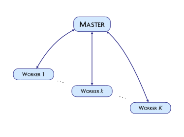
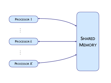
Figure 1. Two commonly used distributed computing architecutures: (a) master-worker (left) and multi-processorwith shared memory (right).

2.1. SGD on Master-Worker Systems

Here we consider the first distributed computing architecture: the master-worker system. The standard way of deploying stochastic gradient descent in such systems – and that which we adopt here – is for the workers to asychronously compute stochastic gradients and then send them to the master, while the master updates the global state of the system and pushes the updated state back to the workers ([1, 31]). This process is presented in Algorithm 1.

Algorithm 1 Running SGD on a Master-Worker Architecture

0:  $1$ Master and $K$ workers, $k=1,\dotsc,K$

1:  Each worker is seeded with the same inital iterate

2:  repeat

3:     Master: (a) Receive a stochastic gradient from worker $k$ (b) Update current iterate. (c) Send updated iterate to worker $k$

4:     Workers: (a) Receive iterate (b) Compute an i.i.d. stochastic gradient (at the received iterate) (c) Send the computed gradient to master

5:  until end

Due to the distributed nature of the master-worker system, a gradient received by the master on any given iteration can be stale. As a simple example, consider a fully coordinated update scheme where each worker sends the computed gradient to and receives the updated iterate from the master following a round-robin schedule. In this case, each worker’s gradient is received with a delay exactly equal to $K-1$ ($K$ is the number of workers in the system), because by the time the master receives worker $K$’s computed gradient, the master has already applied $K-1$ gradient updates from workers $1$ to $K-1$ (and since the schedule is round-robin, this delay of $K-1$ is true for any one of the $K$ workers).

However, delays can be much worse since we allow full asynchrony: workers can compute and send (stochastic) gradients to the master without any coordinated schedule. In the asynchronous setting, fast workers (workers that are fast in computing gradients) will cause disproprotionately large delays to gradients produced by slow workers (workers that are slow in computing gradients): when a slower worker has finished computing a gradient, a fast worker may have already computed and communicated many gradients to the master. Since the master updates the global state of the system (the current iterate), one can gain a clearer representation of this scheme by looking at the master’s update. This is given in Section 2.3.

2.2. SGD on Multi-Processor Systems with Shared Memory

Here we consider the second distributed computing architecture: multi-processor system with shared memory. In this architecture, all processors can access a global, shared memory, which holds all the data needed for computing a (stochastic) gradient, as well as the current iterate (the global state of the system). The standard way of deploying stochastic gradient descent in such systems ([11, 31]) is for each processor to independently and asychronously read the current global iterate, compute a stochastic gradient , and then update the global iterate in the shared memory. This process is given Algorithm 2:

Algorithm 2 Running SGD on a Multi-Processor System with Shared Memory

0:  $K$ processors and global (shared) memory.

1:  The initial iterate in the global memory.

2:  repeat

3:     (a) Each proceesor reads the current global iterate. (b) Each processor reads data from memory and computes a stochastic gradient. (c) Each processor updates the global iterate.

4:  until end

The key difference from Algorithm 1 is that there is no central entity that updates the global state; instead, each processor can both read the global state and update it. Since each processor is performing the operations asynchronously, different processors may be reading the same global iterate at the same time. Further, the delays in this case is again caused by the heterogeneity across different processors: if a processor is slow in computing gradients, then by the time it finishes computing its gradient, the global iterate has been updated by other, faster processors many times over, thereby causing its own gradient stale. Here, we also adopt a common assumption that updating the global iterate is an atomic operation (and hence no two processors will be updating the global iterate at the same time). This is justified because performing gradient update is a simple arithemtic operation, and hence takes negligible time compared to reading data and computing a stochastic gradient, which is the main computational bottleneck in practice. However, despite a cheap computation, performing the whole gradient update (typically achieved via locking) does have overhead. In particular, a less stringent model would be only updating one coordinate at a time: this is known as an inconsistent write/read model since different processors are updating different components of the global parameters and hence can read in elements of different ages. For simplicity, we do not consider this case, as our focus in this paper is on delays. See [31] and [34] for lucid discussions and analyses on this model. Finally, one can gain a clearer picture of this update scheme by tracking the update to the global iterate in the shared memory. This is given in Section 2.3.

2.3. DASGD: A Unifying Algorithmic Representation

In this subsection, we present a unified algorithmic description, aptly called distributed asynchronous stochastic gradient descent (DASGD), that formally captures both Algorithm 1 and Algorithm 2, where their differences are reflected in the assumptions of the meta algorithm’s parameters. We start with the unconstrained case, see Algorithm 3.

Algorithm 3 Distributed asynchronous stochastic gradient descent

0:  Initial state $X_{0}\in\mathbb{R}^{d}$, step-size sequence $\alpha_{n}$

1:  $n\leftarrow 0$;

2:  repeat

3:     $X_{n+1}=X_{n}-\alpha_{n+1}\nabla F(X_{s(n)},\omega_{n+1})$;

4:     $n\leftarrow n+1$;

5:  until end

6:  return solution candidate $X_{n}$

Algorithm 4 Distributed asynchronous stochastic gradient descent with projection

0:  Initial state $Y_{0}\in\mathbb{R}^{d}$, step-size sequence $\alpha_{n}$

1:  $n\leftarrow 0$;

2:  repeat

3:     $X_{n}=\operatorname{\mathbf{pr}_{\mathcal{X}}}(Y_{n})$;

4:     $Y_{n+1}=Y_{n}-\alpha_{n+1}\nabla F(X_{s(n)},\omega_{n+1})$;

5:     $n\leftarrow n+1$;

6:  until end

7:  return solution candidate $X_{n}$

In more detail, $n$ is a global counter and is incremented every time an update occurs to the current solution candidate $X_{n}$ (the global iterate): in the master-worker systems, the master updates it; in the multi-processor systems, each processor updates it. Since there are delays in both systems, the gradient applied to the current iterate $X_{n}$ can be a gradient associated with a previous time step. This fact is abstractly captured by Line 3 in Algorithm 4. In full generality, we will write $s(n)$ for the iteration from which the gradient received at time $n$ originated. In other words, the delay associated with iteration $s(n)$ is $n-s(n)$, since it took $n-s(n)$ iterations for the gradient computed on iteration $s(n)$ to be received at stage $n$. Note that $s(n)$ is always no larger than $n$; and if $n=s(n)$, then there is no delay in iteration $n$.

Now, the difference between the two distributed computing archecitures is reflected in the assumption of $s(n)$. Specifically, in the master-worker systems, each $s(\cdot)$ is a one-to-one function, because no two workers will ever receive same iterates from the master per Algorithm 1. On the other hand, in multi-processor systems, $s(n)$ can be the same for different $n$’s (since different processors may read the current iterate at the same time); however, it is easy to observe that the same $s$ will appear at most $K$ times for different $n$’s, since there are $K$ processors in total. As an important note, our analysis is agnostic to whether $s(n)$ is one-to-one or not. Consequently, in establishing theoretical guarantees for the meta algorithm DASGD, we obtain the same guarantees for both architectures simultaneously.

Notation-wise, we will write $d_{n}$ for the delay required to compute a gradient requested at iteration $n$. This gradient is received at iteration $n+d_{n}$. Following this notation, the delay for a gradient received at $n$ is $d_{s(n)}=n-s(n)$. Note also we have chosen the subscript associated with $\omega$ to be $n+1$: we can do so because $\omega_{n}$’s are iid (and hence the indexing is irrelevant). Finally, in constrained optimization case (where $\mathcal{X}$ is a strict subset of $\mathbb{R}^{d}$), projection must be performed. This results in DASGD with projection, which is formally given in Algorithm 4.

3. General Nonconvex Objectives

In this section, we take $\mathcal{X}=\mathbb{R}^{d}$ (i.e. unconstrained optimization) and consider general non-convex objectives. Note that for a general non-convex objective where no further structural assumption (e.g. convexity) is made, convergence to an optimal solution (even a local optimal solution) cannot be expected, and will not hold in general, even in the absence of both noise and delays (i.e. single machine deterministic optimization). In such cases, the best one can hope for, which is also the standard metric to determine the stability of the algorithm, is that the gradient vanishes in the limit.

3.1. Delay Assumption

Our goal here is to establish convergence guarantees (in mean square) of DASGD for a general non-convex objective in the presence of delays. In fact, a large family of unbounded delay processes can be tolerated. We state our main assumption regarding the delays and step-sizes:

Assumption 2.

The gradient delay process $d_{n}$ and the step-size sequence $\alpha_{n}$ of DASGD (Algorithms 3 and 4) satisfy one of the following conditions:

1. Bounded delays: $\sup_{n}d_{n}\leq D$ for some positive number $D$ and $\sum_{n=1}^{\infty}\alpha_{n}^{2}<\infty$, $\sum_{n=1}^{\infty}\alpha_{n}=\infty$.

2. Sublinearly growing delays: $d_{n}=O(n^{p})$ for some $0<p<1$ and $\alpha_{n}\propto 1/n$.

3. Linearly growing delays: $d_{n}=\operatorname{\mathcal{O}}(n)$ and $\alpha_{n}\propto 1/(n\log n)$.

4. Polynomially growing delays: $d_{n}=\operatorname{\mathcal{O}}(n^{q})$ for some $q\geq 1$ and $\alpha_{n}\propto 1/(n\log n\log\log n)$.

Note that as delays get larger, we need to use less aggressive step-sizes. This is to be expected, because the larger the delays, the more “averaging" one needs perform in order to remove the staleness that is caused by the delays; and smaller step-sizes correspond to averaging over a longer horizon. This is a one of the important insights that occur throughout the paper. Another thing to note that is the Assumption 2 also highlights the quantitative relationship between the class of delays and the class of step-sizes. For instance, when the delays increase from a linear rate to a polynomial rate, only a factor of $\frac{1}{\log\log n}$ needs to be added (which is effectively a constant). From a practical standpoint, this means that a step-size on the order of $1/(n\log n)$ will be a good model-agnostic choice and more-or-less sufficient for almost all delay processes.

3.2. Controlling the Tail Behavior of Second Moments

We now turn to establish the theoretical convergence guarantees of DASGD for general non-convex objectives. Our first step lies in controlling the tail behavior of the second moments of the gradients that are generated from DASGD. By leveraging the Lipschitz continuity of the gradient, its telescoping sum, appropriate conditionings and a careful analysis of the interplay between delays and step-sizes, we show that (next lemma) a particularly weighted tail sum of the second moments are vanishingly small in the limit (see appendix for a detailed proof).

Lemma 1.

Under Assumptions 1 and 2, if $\inf_{x\in\mathcal{X}}f(x)>-\infty$, then

$$\sum_{n=0}^{\infty}\alpha_{n+1}\operatorname{\mathbb{E}}[\|\operatorname{\nabla}f(X_{n})\|_{2}^{2}]<\infty.$$ (2)

Remark 2.

Since $\sum_{n=0}^{\infty}\alpha_{n+1}=\infty$, Lemma 1 implies that $\lim\inf_{n\rightarrow\infty}\operatorname{\mathbb{E}}[\|\operatorname{\nabla}f(X_{n})\|_{2}^{2}]=0$ (see Appendix A of [6]). Note that the converse is not true: when a subsequence of $\operatorname{\mathbb{E}}[\|\operatorname{\nabla}f(X_{n})\|_{2}^{2}]$ converges to $0$, the sum in Equation (5) need not be finite. As a simple example, consider $\alpha_{n+1}=\frac{1}{n}$, and

$$\operatorname{\mathbb{E}}[\|\operatorname{\nabla}f(X_{n})\|_{2}^{2}]=\begin{cases}\frac{1}{n},\text{ if }n=2^{k}\\ 1,\text{ otherwise}.\end{cases}$$ (3)

Then the subsequence on indicies $2^{n}$ converges to $0$, but the sum still diverges. Consequently, Lemma 1 is stronger than subsequence convergence.

3.3. Bounding the Successive Differences

However, Lemma 1 is still not strong enough to guarantee that $\lim_{n\rightarrow\infty}\operatorname{\mathbb{E}}[\|\operatorname{\nabla}f(X_{n})\|_{2}^{2}]=0$. This is because the convergent sum given in Equation (5) only limits the tail growth somewhat, but not completely. To demonstrate this point, let $c_{t}$ be the following boolean variable:

$$c_{n}=\begin{cases}1,\text{ if $n$ contains the digit $9$ in its decimal expansion,}\\ 0,\text{ otherwise}.\end{cases}$$ (4)

For instance, $c_{9}=1$, $c_{11}=0$. Now define $\alpha_{n+1}=\frac{1}{n}$, and $\operatorname{\mathbb{E}}[\|\operatorname{\nabla}f(X_{n})\|_{2}^{2}]=\begin{cases}\frac{1}{n},\text{ if }c_{n}=1\\ 1,\text{ if }c_{n}=0.\end{cases}$ As first-year Berkeley Math PhDs delightfully found out during– or painfully found out after – their qualifying exam, $\sum_{n=1}^{\infty}\alpha_{n+1}\operatorname{\mathbb{E}}[\|\operatorname{\nabla}f(X_{n})\|_{2}^{2}]<\infty$ (see Problem 1.3.24 in [12]), even though the limit $\operatorname{\mathbb{E}}[\|\operatorname{\nabla}f(X_{n})\|_{2}^{2}]$ does not exist. This indicates that to obtain convergence of $\operatorname{\mathbb{E}}[\|\operatorname{\nabla}f(X_{n})\|_{2}^{2}]$, we need to impose more stringent conditions to ensure its sufficient tail decay. Note that one issue that is revealed by the above counter-example is that the distance between two successive terms is always bounded away from $0$, no matter how large $n$ is. This obviously makes it possible for convergence to occur: a necessary condition for convergence is that the difference converges to $0$. Note that intuitively, this pathological case cannot occur for gradient descent, because the step-size is shrinking to $0$, hence making the successive difference converge to $0$ (at least in expectation). Consequently, we can bound the difference between every two successive terms in terms of a decreasing sequence that is converging to $0$. This ensures that $\operatorname{\mathbb{E}}[\|\operatorname{\nabla}f(X_{n})\|_{2}^{2}]$ cannot change two much from iteration to iteration. Further, the change between two successive terms will be vanishing. This result is formalized in the following lemma (the proof is given in the appendix):

Lemma 2.

Under Assumptions 1 and 2, there exists a constant $C>0$ such that for every $n$,

$$\Big{|}\operatorname{\mathbb{E}}[\|\operatorname{\nabla}f(X_{n+1})\|_{2}^{2}]-\operatorname{\mathbb{E}}[\|\operatorname{\nabla}f(X_{n})\|_{2}^{2}]\Big{|}\leq C\alpha_{n+1}.$$

3.4. Main Convergence Result

Putting the above two characterizations together, we obtain:

Theorem 1.

Let $X_{n}$ be the DASGD iterates generated from Algorithm 3. Under Assumptions 1 and 2, if $\inf_{x\in\mathcal{X}}f(x)>-\infty$, then

$$\lim_{n\to\infty}\operatorname{\mathbb{E}}[\|\operatorname{\nabla}f(X_{n})\|_{2}^{2}]=0.$$ (5)

Remark 3.

Three remarks are in order here. First, note that the condition $\inf_{x\in\mathcal{X}}f(x)>-\infty$ means that the optimization problem (Opt) has a solution. This is necessary, because otherwise, a stationary point may not exist in the first place, and DASGD (or even simple gradient descent) may continue decrease the objective value ad infinitum. Note that since $f$ is smooth, a minimum point is necessarily a stationary point.

Second, the above convergence is a fairly strong characterization of the fact that the gradient vanishes. In particular, it means that the gradient of the DASGD iterates converges to $0$ in mean square. Consequently, this implies that the norm of the gradient vanishes in expectation, and that the gradient converges to $0$ with high probability. Note further that if we strengthen Assumption 1 to require that all stochastic gradients are bounded almost surely (as opoosed to just bounded in second moments), then a similar analysis ensures almost sure convergence of $\|\operatorname{\nabla}f(X_{n})\|_{2}$. We omit the details due to space limitation. Finally, that Theorem 1 is a direct consequence of Lemmas 1 and 2 is a simple excercise in elementary series theory (in particular, Lemma A.4).

4. Variationally Coherent Problems

In this section, our goal is to establish global optimality convergence guarantees of DASGD in as wide a class of optimization problems as possible. Since global convergence cannot be expected to hold for all non-convex optimization problems (even without delays). a standard structural assumption to make in the existing literature on the objectives (even in the no-delay case) is convexity. Here we instead consider a much broader class of stochastic optimization problems than convex problems. Further, we allow for constrained optimization; in particular, $\mathcal{X}$ is assumed to be a convex and compact subset of $\mathbb{R}^{d}$ throughout the section. We first discuss the class of objectives and then present global convergence results and their analyses in the subsequent two subsections. We focus on the class of mean variationally coherent optimization problems [57, 38, 37, 58], defined here as follows:

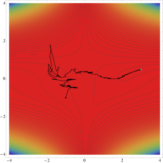
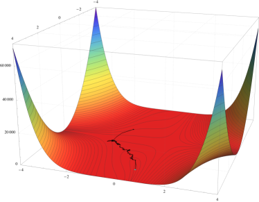
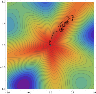
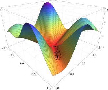
Figure 2. Examples of variationally coherent objectives: on the top row, the Beale function $f(x_{1},x_{2})=(1.5-x_{1}+x_{1}x_{2})^{2}+(2.25-x_{1}+x_{1}x_{2}^{2})^{2}+(2.625-x_{1}+x_{1}x_{2}^{3})^{2}$ over the benchmark domain $[-4,4]\times[-4,4]$; on the bottom row, the polar example $f(r,\theta)=(3+\sin(5\theta)+\cos(3\theta))r^{2}(5/3-r)$ over the unit ball $0\leq r\leq 1$. In both figures, the black curves indicate a sample trajectory of DASGD with linearly growing delays.

Assumption 3.

The optimization problem (Opt) is called variationally coherent in the mean if

$$\operatorname{\mathbb{E}}[\langle\operatorname{\nabla}F(x;\omega)\mathopen{},\mathopen{}x-x^{\ast}\rangle]\geq 0,$$ (VC)

for all $x^{\ast}\in\mathcal{X}^{\ast}$ and all $x\in\mathcal{X}$ with equality only if $x\in\mathcal{X}^{\ast}$.

Note that we do not impose the “if" condition for equality: if $x\in\mathcal{X}^{\ast}$, then the equality may or may not hold. By Assumption 1, we can interchange expectation and differentiation in (VC) to obtain

$$\langle\nabla f(x)\mathopen{},\mathopen{}x-x^{\ast}\rangle\geq 0,$$ (6)

for all $x\in\mathcal{X}$, $x^{\ast}\in\mathcal{X}^{\ast}$. As a result, mean variational coherence can be interpreted as an averaged coherence condition for the deterministic optimization problem with objective $f(x)$. Mean variationally coherent optimization problems include convex programs, pseudo-convex programs, non-degenerate quasi-convex programs and star-convex programs as special cases. For instance, if $g$ is star-convex, then $\langle\nabla f(x)\mathopen{},\mathopen{}x-x^{\ast}\rangle\geq f(x)-f(x^{\ast})$ for all $x\in\mathcal{X}$, $x^{\ast}\in\mathcal{X}^{\ast}$. This is easily seen to be a special case of variational coherence because $\langle\nabla f(x)\mathopen{},\mathopen{}x-x^{*}\rangle\geq f(x)-f(x^{*})\geq 0$, with the last inequality strict unless $x\in\mathcal{X}^{*}$. Note that star-convex functions contain convex functions as a subclass (but not necessarily pseudo/quasi-convex functions). See [56, 57] for a more detailed discussion on why these various classes of optimization problems are special cases. Fig. 2 also provides two more elaborate examples of a variationally coherent optimization problem that are not quasi-convex. Put together, these examples indicate that variationally coherent objectives can have highly non-convex profiles. Nevertheless, for the class of variationally coherent functions, it is possible to establish almost sure convergence guarantees (which we do so in the subsequent sections).

4.1. Deterministic Analysis: Convergence to Global Optima

To streamline our presentation and build intuition along the way, we will begin with the deterministic case in this subsection, where there is no randomness in the calculation of a gradient update. In this case, DASGD boils down to distributed asynchronous gradient descent (DAGD), as illustrated in Algorithm 5:

Algorithm 5 Distributed Asynchronous Gradient Descent (DAGD)

0:  Initial state $y_{0}\in\mathbb{R}^{d}$, step-size sequence $\alpha_{n}$

1:  $n\leftarrow 0$

2:  repeat

3:     $x_{n}=\operatorname{\mathbf{pr}_{\mathcal{X}}}(y_{n})$;

4:     $y_{n+1}=y_{n}-\alpha_{n+1}\nabla f(x_{s(n)})$;

5:     $n\leftarrow n+1$;

6:  until end

7:  return solution candidate $x_{n}$

4.1.1. Energy Function

We start with an energy function that measures on how “optimal" the dual variable $y$ is: the smaller the energy (i.e. the closer it is to $0$), the better the dual variable.

Definition 1.

Let $x^{\ast}\in\mathcal{X}^{\ast}$. Define the energy function $E\colon\mathbb{R}^{d}\to\mathbb{R}$ as follows:

$$E(y)=\inf_{x^{\ast}\in\mathcal{X}^{\ast}}E_{x^{\ast}}(y),\text{ where }E_{x^{\ast}}(y)=\lVert x^{\ast}\rVert_{2}^{2}-\lVert\operatorname{\mathbf{pr}_{\mathcal{X}}}(y)\rVert_{2}^{2}+2\langle y\mathopen{},\mathopen{}\operatorname{\mathbf{pr}_{\mathcal{X}}}(y)-x^{\ast}\rangle.$$ (7)

Note that one can think of $E_{x^{\ast}}(y)$ as the energy of $y$ with respect to a fixed optimal solution $x^{\ast}$, while $E(y)$ is the best (smallest) energy for a given $y$. We next characterize a few of its useful properties.

Lemma 3.

For all $y\in\mathbb{R}^{d}$, we have:

1. $E(y)\geq 0$ with equality if and only if $\operatorname{\mathbf{pr}_{\mathcal{X}}}(y)\in\mathcal{X}^{\ast}$.

2. Let $\{y_{n}\}_{n=1}^{\infty}$ be a given sequence. If $\lim_{n\to\infty}E(y_{n})=0$, then $\operatorname{\mathbf{pr}_{\mathcal{X}}}(y_{n})\rightarrow\mathcal{X}^{\ast}$ as $n\to\infty$.

Remark 4.

The proof is given in the appendix, but it is helpful to make a few quick remarks. The first statement justifies the terminology of “energy", as $E(y)$ is always non-negative. This energy function will also be the tool we use to establish an important component of the global convergence result. Further, given that $E(y)\geq 0$, it should also be clear that when $\operatorname{\mathbf{pr}_{\mathcal{X}}}(y)\in\mathcal{X}^{\ast}\subset\mathcal{X}$, we can choose a particular $x^{\ast}=\operatorname{\mathbf{pr}_{\mathcal{X}}}(y)$ such that $E(y)=0$ (but that $E(y)=0$ implies $\operatorname{\mathbf{pr}_{\mathcal{X}}}(y)\in\mathcal{X}^{\ast}$ is less obvious). Statement 2 of the lemma provides us with a way to establish convergence to optimal solutions. If we can show that $E(y_{n})\to 0$, then $x_{n}=\operatorname{\mathbf{pr}_{\mathcal{X}}}(y_{n})\to\mathcal{X}^{\ast}$. Nevertheless, as we shall see later, unlike many other Lyapunov functions in optimization, $E(y_{n})$ does not decrease monotonically; consequently, it is difficult to directly establish $E(y_{n})\to 0$. In fact, a finer-grained analysis is required to characterize the convergence behavior of $E(y_{n})$ (see Section 4.1.2).

We also assume that the converse of Statement 2 of the above lemma holds:

Assumption 4.

If $\lim_{n\to\infty}E(y_{n})=0$, then $\operatorname{\mathbf{pr}_{\mathcal{X}}}(y_{n})\rightarrow\mathcal{X}^{\ast}$ as $n\rightarrow\infty$.

Assumption 4 can be seen as a primal-dual analogue of the reciprocity conditions for the Bregman divergence. This assumption usually holds (e.g. when the feasible set $\mathcal{X}$ is a polytope), unless $\mathcal{X}$ is pathological.

Lemma 4.

Fix any $x^{\ast}\in\mathcal{X}^{\ast}$.

1. $\|\operatorname{\mathbf{pr}_{\mathcal{X}}}(y)-\hat{y}\|_{2}^{2}-\|\operatorname{\mathbf{pr}_{\mathcal{X}}}(\hat{y})-\hat{y}\|_{2}^{2}\leq\|y-\hat{y}\|_{2}^{2}$, for any $y,\hat{y}\in\mathbb{R}^{d}$.

2. $E_{x^{\ast}}(y+\Delta y)-E_{x^{\ast}}(y)\leq 2\langle\Delta y,\operatorname{\mathbf{pr}_{\mathcal{X}}}(y)-x^{*}\rangle+\|\Delta y\|_{2}^{2}$, for any $y,\Delta y\in\mathbb{R}^{d}$.

Remark 5.

The first statement of the above lemma serves as an important intermediate step in proving the second statement, and is established by leveraging the envelop theorem and several important properties of Euclidean projection. To see that this is not trivial, consider the quantity $\|\operatorname{\mathbf{pr}_{\mathcal{X}}}(y)-\hat{y}\|_{2}-\|\operatorname{\mathbf{pr}_{\mathcal{X}}}(\hat{y})-\hat{y}\|_{2}$, which we know by triangle’s inequality satisfies:

$$\begin{split}&\|\operatorname{\mathbf{pr}_{\mathcal{X}}}(y)-\hat{y}\|_{2}-\|\operatorname{\mathbf{pr}_{\mathcal{X}}}(\hat{y})-\hat{y}\|_{2}\leq\|\operatorname{\mathbf{pr}_{\mathcal{X}}}(y)-\operatorname{\mathbf{pr}_{\mathcal{X}}}(\hat{y})\|_{2}\leq\|y-\hat{y}\|_{2},\end{split}$$ (8)

where the last inequality follows from the fact that projection is a non-expansive map. However, this inequality is not sufficient for our purposes because in quantifying the perturbation $E(y+\Delta y)-E(y)$, we also need the squared term $\|\Delta y\|_{2}^{2}$, which is not easily obtainable from Equation (8). In fact, a tighter analysis is needed to establish that $\|y-\hat{y}\|_{2}^{2}$ is an upper bound on $\|\operatorname{\mathbf{pr}_{\mathcal{X}}}(y)-\hat{y}\|_{2}^{2}-\|\operatorname{\mathbf{pr}_{\mathcal{X}}}(\hat{y})-\hat{y}\|_{2}^{2}$.

4.1.2. Main Convergence Result

An intermediate result, interesting on its own and useful also as a heavy-lifting tool for our convergence analysis is then provided by the following technical result:

Proposition 1.

Under Assumptions 1, 3, 2 and 4, DAGD admits a subsequence $x_{n_{k}}$ that converges to $\mathcal{X}^{\ast}$ as $k\to\infty$.

We highlight the main steps below and refer the reader to the appendix for the details:

1. Letting $b_{n}=\operatorname{\nabla}f(x_{s(n)})-\operatorname{\nabla}f(x_{n})$, we can rewrite the gradient update in DAGD as:

   $$y_{n+1} =y_{n}-\alpha_{n+1}\operatorname{\nabla}f(x_{s(n)})$$

   $$=y_{n}-\alpha_{n+1}\operatorname{\nabla}f(x_{n})-\alpha_{n+1}\{\operatorname{\nabla}f(x_{s(n)})-\operatorname{\nabla}f(x_{n})\}$$

   $$=y_{n}-\alpha_{n+1}(\operatorname{\nabla}f(x_{n})+b_{n}).$$ (9)

   Recall here that $s(n)$ denotes the previous iteration count whose gradient becomes available only at the current iteration $n$. By bounding the magnitude of $b_{n}$ using the delay sequence through a careful analysis, we establish that under any one of the conditions in Assumption 2, $\lim_{n\to\infty}\|b_{n}\|_{2}=0$. The analysis here, particularly the one for the last three conditions, reveals the following pattern: as the magnitude of the delays gets larger and larger in the order of growth, one needs to use a more conservative step-size sequence in order to mitigate the damage done by the stale gradient information. Intuitively, smaller step-sizes are more helpful in larger delays because they carry a better “amortization" effect that makes DAGD more tolerant to delays.

2. With the defintion of $b_{n}$, DAGD can be written as:

   $$x_{n} =\operatorname{\mathbf{pr}_{\mathcal{X}}}(y_{n}),$$ (10)

   $$y_{n+1} =y_{n}-\alpha_{n+1}(\operatorname{\nabla}f(x_{n})+b_{n}).$$

   We then use the energy function to study the behavior of $y_{n}$ and $x_{n}$. More specifically, we look at the quantity $E(y_{n+1})-E(y_{n})$ and, using Lemma 4, we bound this one-step change using the step size $\alpha_{n}$, the $b_{n}$ sequence and the defining quantity $\langle\operatorname{\nabla}f(x_{n}),x_{n}-x^{*}\rangle$ of a variationally coherent function (as well as another term that will prove inconsequential). We then telescope on $E(y_{n+1})-E(y_{n})$ to obtain an upper bound for $E(y_{n+1})-E(y_{0})$. Since the energy function is always non-negative, $E(y_{n+1})-E(y_{0})$ is at least $-E(y_{0})$ for every $n$. Then, utilizing the fact that $b_{n}$ converges to $0$ and that $\langle\operatorname{\nabla}f(x_{n}),x_{n}-x^{*}\rangle$ is always positive (unless the iterate is exactly an optimal solution, in which case it is $0$), we show that the upper bound will approach $-\infty$ if $X_{n}$ only enters $\mathcal{N}(\mathcal{X}^{\ast},\epsilon)$, an open $\epsilon$-neighborhood of $\mathcal{X}^{\ast}$, a finite number of times (for an arbitrary $\epsilon>0$). This generates an immediate contradiction, and thereby establishes that $X_{n}$ will get arbitrarily close to $\mathcal{X}^{\ast}$ for an infinite number of times. This then implies that there exists a subsequence of DAGD iterates that converges to the solution set of (Opt), i.e, $x_{n_{k}}\to\mathcal{X}^{\ast}$ as $k\to\infty$.

Theorem 2.

Under Assumptions 1, 3, 2 and 4, the global state variable $x_{n}$ of DAGD (Algorithm 5) converges to the solution set $\mathcal{X}^{\ast}$ of (Opt).

We give an outline of the proof below, referring to the appendix for the details.

Fix a $\delta>0$. Since $x_{n_{k}}\to x^{*}$, as $k\to\infty$ (per Proposition 1), we have $E(y_{n_{k}})\to 0$ as $k\to\infty$ per Lemma 3. So we can pick an $n$ that is sufficiently large and $E(y_{n})<\delta$. Our goal here is to show that for $n$ large enough, once $E(y_{n})<\delta$, it will stay so forever: $E(y_{m})<\delta,\forall m\geq n$. Note in particular that the above statement is not true for all $n$, but only for $n$ large enough.

However, the behavior of $E(y_{n})$ is not very regular: it can certainly increase from iteration to iteration for any $n$. Nevertheless, we can precisely quantify how large this increment (if any) can be. This leads us to break it down to two cases:

1. Case 1: $E(y_{n})<\delta/2$.

2. Case 2: $\delta/2\leq E(y_{n})<\delta$.

For Case 1, we show in the appendix that

$$E{(y_{n+1})}-E(y_{n})\leq 2BC_{4}\alpha_{n+1}+2\alpha_{n+1}^{2}(C_{2}+B^{2}),$$ (11)

for suitable constants $B$ and $C$‘s. Now for $n$ sufficiently large, we can make the right-hand arbitrarily small, and in particular, smaller than $\delta/2$. This means $E{(y_{n+1})}\leq E{(y_{n})}+\frac{\delta}{2}<\delta$. Consequently, in this case, the energy stays within the $\delta$ bound in the next iteration.

For Case 2, we show in the appendix that

$$E{(y_{n+1})}-E(y_{n})\leq-2\alpha_{n+1}\left[\frac{a}{2}-\alpha_{n+1}(C_{2}+B^{2})\right],$$ (12)

where $a$ is a positive constant that depends only on $\delta$. Again, since $n$ is sufficiently large, we can make $\frac{a}{2}-\alpha_{n+1}(C_{2}+B^{2})$ positive, thereby making the right-hand side negative. Consequently, $E{(y_{n+1})}<E(y_{n})<\delta$. Hence, again, the energy stays within the $\delta$ bound in the next iteration.

The key conclusion from the above is that, for large enough $n$, once $E{(y_{n})}$ is less than $\delta$, $E(y_{n+1})$ is less than $\delta$ as well and so are all the iterates afterwards. Since $\delta$ is arbitrary, it follows $E{(y_{n})}\to 0$, and therefore $x_{n}\to\mathcal{X}^{\ast}$ by Lemma 3.

4.2. Stochastic Analysis: Almost Sure Convergence to Global Optima

Having established deterministic global convergence of DAGD, we now proceed to study stochastic global convergence of DASGD. Compared to the deterministic analysis, the stochastic case is much more involved because randomness can lead to very volatile behavior in the presence of delays; in particular, the simple approach employed in Theorem 2 (to establish that once $E{(y_{n})}$ is less than $\delta$, it will always remain so) no longer works. To deal with both delays and noise, a much more sophisticated analysis framework needs to be developed, which requires several news ideas. To streamline our presentation, we break the theoretical development into four subsections, each comprising an important component and step of the overall analysis.

4.2.1. Recurrence of DASGD

Our first step lies in generalizing Proposition 1 to the stochastic case. Specifically, in the presence of noise, we show that the iterates of DASGD visit any neighorhood of $\mathcal{X}^{\ast}$ infinitely often almost surely.

Proposition 2.

Under Assumptions 1, 3, 2 and 4, DASGD admits a subsequence $X_{n_{k}}$ that converges to $\mathcal{X}^{\ast}$ almost surely: $X_{n_{k}}\to\mathcal{X}^{\ast}$ with probability $1$ as $k\to\infty$.

We outline the two main steps of the proof below, referring the reader to the appendix for the details.

1. We begin by rewriting the gradient update step in DASGD as:

   $$\frac{Y_{n+1}-Y_{n}}{\alpha_{n+1}} =-\nabla F(X_{s(n)},\omega_{n+1})$$

   $$=-\operatorname{\nabla}f(X_{n})$$

   $$-[\operatorname{\nabla}f(X_{s(n)})-\operatorname{\nabla}f(X_{n})]$$

   $$-[\nabla F(X_{s(n)},\omega_{n+1})-\operatorname{\nabla}f(X_{s(n)})].$$ (13)

   Letting $B_{n}=\operatorname{\nabla}f(X_{s(n)})-\operatorname{\nabla}f(X_{n})$ and $U_{n+1}=\nabla F(X_{s(n)},\omega_{n+1})-\operatorname{\nabla}f(X_{s(n)})$, we can rewrite the DASGD update as

   $$Y_{n+1}=Y_{n}-\alpha_{n+1}\{\operatorname{\nabla}f(X_{n})+B_{n}+U_{n+1}\}.$$ (14)

   We then establish the following two facts in this step. First, we verify that $\sum_{r=0}^{n}U_{n+1}$ is a martingale adapted to $Y_{1},Y_{2}\dots,Y_{n+1}$, where $\{U_{n+1}\}_{n=0}^{\infty}$ is a $L_{2}$-bounded martingale difference sequence. Second, we show that $\lim_{n\to\infty}\|B_{n}\|_{2}=0,{a.s.}.$

   The second claim is done by first giving an upper bound on $\|B_{n}\|_{2}$ by writing $\operatorname{\nabla}f(X_{s(n)})-\operatorname{\nabla}f(X_{n})$ as a sum of one-step changes ($\operatorname{\nabla}f(X_{s(n)})-\operatorname{\nabla}f(X_{s(n)+1})+\operatorname{\nabla}f(X_{s(n)+1})-\dots+\operatorname{\nabla}f(X_{n-1})-\operatorname{\nabla}f(X_{n})$) and analyzing each such successive change. We then break that upper bound into two parts, one deterministic and one stochastic. For the deterministic part, the same analysis in the proof of Proposition 1 yields convergence to $0$.

   The stochastic part turns out to be the tail of a martingale. By leveraging the property of the step-size and a crucial property of martingale differences (two martingale differences at different time steps are uncorrelated), we establish that said martingale is $L_{2}$-bounded. Then, by applying a version of Doob’s martingale convergence theorem, it follows that said martingale converges almost surely to a limit random variable with finite second moment (and hence almost surely finite). Consequently, writing the tail as a difference between two terms (each of which converges to the same limit variablewith probability $1$), we conclude that the tail converges to $0$ (a.s.).

2. The full DASGD update may then be written as

   $$X_{n} =\operatorname{\mathbf{pr}_{\mathcal{X}}}(Y_{n})$$

   $$Y_{n+1} =Y_{n}-\alpha_{n+1}[\operatorname{\nabla}f(X_{n})+B_{n}+U_{n+1}].$$ (15)

   As in Step 2 of the proof of Proposition 1, we again bound the one-step change of the energy function $E(Y_{n+1})-E(Y_{n})$ and then telescope the differences. The two distinctions from the determinstic case are: 1) Everything is now a random variable. 2) We have three terms: in addition to the random gradient $\operatorname{\nabla}f(X_{n})$ and the random drift $B_{n}$, we also have a martingale term $U_{n+1}$. Since $B_{n}$ converges to $0$ almost surely (as shown in the previous step), its effect can be shown to be negligible. Futher, the analysis utilizes law of large numbers for martingale as well as Doob’s martingale convergence theorem to bound the effect of the various martingale terms and to establish that the final dominating term converges to $-\infty$ almost surely (which generates a contradiction since the energy function is always positive) unless a subsequence $X_{n_{k}}$ converges almost surely to $\mathcal{X}^{\ast}$. $\blacksquare$

Even though recurrence, which can be seen as the counterpart of Proposition 1, holds as per the above proposition, the random iterates $X_{n}$ are much more irregular than their deterministic counterpart $x_{n}$ in DAGD. To deal with this complexity, we work with and characterize the sample trajectories “generated" (to be made precise later) by $X_{n}$ (rather than individual iterates $X_{n}$). To work towards this general direction, we first push the DASGD update into a determinstic ordineary differential equation (ODE), as explained in the next subsection.

4.2.2. Mean-Field Approximation of DASGD

We can rewrite the DASGD update as:

$$X_{n} =\operatorname{\mathbf{pr}_{\mathcal{X}}}(Y_{n})$$

$$Y_{n+1} =Y_{n}-\alpha_{n+1}\{\operatorname{\nabla}f(X_{n})+B_{n}+U_{n+1}\}.$$ (16)

Written in this way, DASGD can be viewed as a discretization of the “mean-field” ODE

$$x =\operatorname{\mathbf{pr}_{\mathcal{X}}}(y),$$

$$\dot{y} =-\operatorname{\nabla}f(x).$$ (17)

The intuition is that this ODE provides a “mean" approximation of the DASGD update, because in (4.2.2), the noise term $U_{n+1}$ has $0$ mean, and the term $B_{n}$ converges to $0$ (and therefore has negilible effect in the long run). Thes leaves only the term $Y_{n+1}=Y_{n}-\alpha_{n+1}\operatorname{\nabla}f(X_{n})$, which can be seen as a Euler discretization of the ODE. (Of course, that Equation (4.2.2) is a good-enough approximation of Equation (4.2.2) for global almost sure convergence purposes here will be rigorously justified later.)

Next, writing Equation (4.2.2) solely in terms of $y$ yields $\dot{y}=-\operatorname{\nabla}f(\operatorname{\mathbf{pr}_{\mathcal{X}}}(y))$. Since $\operatorname{\nabla}f$ and $\operatorname{\mathbf{pr}_{\mathcal{X}}}$ are both Lipschitz continuous and $\mathcal{X}$ is a compact set, the composition $\operatorname{\nabla}f\circ\operatorname{\mathbf{pr}_{\mathcal{X}}}$ is itself Lipschitz continuous and bounded. Standard results from the theory of dynamical systems then show that (4.2.2) admits a unique global solution $y(t)$ for any initial condition $y(0)$. On the other hand, since $\operatorname{\mathbf{pr}_{\mathcal{X}}}$ is not a one-to-one map, it is not invertible; consequently, there need not exist a unique solution trajectory for $x(t)$. By this token, the rest of our analysis will focus on the trajetory of $y(t)$.

With the guarantee of the existence and uniqueness of the $y$ trajectory, let $P\colon\mathbb{R}_{+}\times\mathbb{R}^{d}\to\mathbb{R}^{d}$ be the semiflow of (4.2.2), i.e., $P(t,y_{0})$ denotes the state of (4.2.2) at time $t$ when the initial condition is $y_{0}$. In other words, when viewed as a function of time, $P(\cdot,y_{0})$ is the solution trajectory to $\dot{y}=-\operatorname{\nabla}f(\operatorname{\mathbf{pr}_{\mathcal{X}}}(y))$. It is worth pointing out that writing it in this double-argument form also allows us to interpret $P$ as a function of the initial condition: for a fixed $t$, $P(t,\cdot)$ gives different states at $t$ when the ODE starts from different initial conditions (in particular, $P(0,y)=y$). Both views will be useful later.

It turns out that with the energy function introduced here, $E(P(t,y))$ is always non-increasing. Furthermore, it is also decreasing at a meaingful rate. We end this subsection with a “sufficient decrease” property of the mean dynamics (4.2.2) (the proof given in the appendix due to space limitation):

Lemma 5.

With notation as above, we have:

1. If $\operatorname{\mathbf{pr}_{\mathcal{X}}}(P(t,y))\notin\mathcal{X}^{\ast}$, then $E(P(t,y))$ is strictly decreasing in $t$ for all $y\in\mathbb{R}^{d}$.

2. For all $\delta>0$, there exists some $T\equiv T(\delta)>0$ such that, for all $t\geq T$, we have

   $$\sup\nolimits_{y}\{E(P(t,y))-E(y):E(P(t,y))\geq\delta/2\}\leq-\delta/2.$$ (18)

Lemma 5 essentially says $E(P(t,y))$ is strictly and uniformly (across all $y$) decreasing at a non-vanishing rate. More specifically, to give some intuition of the second part of Lemma 5, note that $E(P(t,y))-E(y)$ is the energy change at time $t$ when starting at $y$. The first part says this quantity is always non-negative. While the second part says provided $E(P(t,y))\geq\delta/2$, the decrease in energy will be at least $\frac{\delta}{2}$, no matter what the initial point $y$ is. If $E(P(t,y))\geq\delta/2$ does not hold, that means the energy at time $t$ is already really small (i.e. $E(P(t,y))<\delta/2$). Consequently, the mantra of the above lemma can be stated succinctly as follows: either the energy is already close to $0$, or the energy will decrease towards $0$.

In fact, by some additional analysis, one can further show that Lemma 5 implies $P(t,y)\to\mathcal{X}^{\ast},\forall y$ as $t\to\infty$. Now, despite being an interesting result on its own (which establishes that the continuous dynamics of DASGD converges to $\mathcal{X}^{\ast}$), it is still some distance away from our final desideratum: our goal is to establish (almost sure) convergence of the discrete-time process in DASGD. So unless we can somehow relate the discrete-time iterates to the continuous-time trajectories, the convergence of DASGD is still uncertain. We fulfill this taks in the next subsection.

4.2.3. Relating DASGD Iterates to ODE Trajectories

Our goal here is to establish a quantitative connection between the DASGD iterates and the ODE trajectory studied in the previous subsection. Our general idea is that if we show the trajectory generated by the discrete-time iterates of DASGD is path-by-path “close" to the continuous-time trajectory $P(t,y)$, then likely almost-sure convergence of the DASGD iterates can be guaranteed as well.

To be more specific, there are two things that need to be more precisely defined from the preceding high-level discussion. First, what does it mean to be a trajectory generated by the discrete-time iterates of DASGD? Second, what does it mean for this trajectory to be “close" to the ODE trajectory? In general, the answers to these questions can vary depend on the specific goal at hand. In the current context, our goal is to establish global almost sure convergence (a very strong result). Consequently, we need to choose the answers rather judiciously: on the one hand, the answers must be stringent enough to ensure global almost sure convergence in the end (for instance, for the second question, a fairly strong notion of “closeness" is needed); on the other hand, they must also be flexible enough to fit in the current context.

As it turns out, the answer to the first question is rather intuitive: (perhaps) the simplest way to generate a continuous trajectory from a sequence of discrete points is the affine interpolation: connect the iterates $Y_{0},Y_{1},\dots,Y_{n}$ at times $0,\alpha_{1},\dots,\sum_{r=1}^{n=1}\alpha_{r}$. We call this curve the affine interpolation curve of DASGD and denote it by $A(t)$. Note that $A(t)$ is a random curve because the DASGD iterates $Y_{0},Y_{1},\dots,Y_{n}$ are random. To avoid confusion, we summarize the three different objects discussed so far:

1. The DASGD iterates $Y_{0},Y_{1},\dots,Y_{n}$.

2. The affine interpolation curve $A(t)$ of $Y_{n}$.

3. The flow $P(t,y)$ of the ODE (4.2.2).

The answer to the second question lies in the notion of an asymptotic pseudotrajectory (APT) , a concept introduced by Benaïm and Hirsch [4] and Benaïm and Schreiber [5]. Specifically, in our current context, a continuous curve $s(t)$ is considered close to ODE solution $P(t,y)$ if the following holds:

Definition 2.

A continuous function $s:\mathbb{R}_{+}\to\mathbb{R}^{d}$ is an APT for $P$ if for every $T>0$,

$$\lim_{t\to\infty}\sup_{0\leq h\leq T}d(s(t+h),P(h,s(t)))=0,$$ (19)

where $d(\cdot,\cdot)$ is the Euclidean metric in $\mathbb{R}^{d}$.

Intuitively, the definition matches exactly the naming: $s$ is an APT for $P$ if, for sufficiently large $t$, the flow lines of $P$ remain arbitrarily close to $s(t)$ over a time window of any (fixed) length. More precisely, for each fixed $T>0$, one can find a large enough $t_{0}$, such that for all $t>t_{0}$, the curve $s(t+h)$ approximates the trajectory $P(h,s(t))$ on the interval $h\in[0,T]$ with any predetermined degree of accuracy.

With this definition in place, to push through the agenda, we need to establish that $A(t)$, the affine interpolation curve of the DASGD iterates, is an APT for the flow $P(t,y)$ induced by the ODE (4.2.2). More precisely, we establish that $A(t)$ is an APT for the flow $P(t,y)$ almost surely, because as mentioned before, $A(t)$ is a random curve.

Lemma 6.

Let $A(t)$ be the random affine interpolation curve generated from the DASGD iterates. Then $A(t)$ is an APT of $P(t,y)$ almost surely.

Note that this result means any resulting affine interpolation curve of DASGD is close to the ODE trajectory. This also forms the basis for reasoning convergence on a path-by-path scale. However, more work still remains to be done because, unfortunately, the condition that $A(t)$ is an APT for $P$ almost surely does not guarantee that the discrete-time iterates of DASGD converge to $\mathcal{X}^{\ast}$ (for many counterexamples in general dynamical systems, see Benaïm [3]). In other words, the notion of APT is not sharp enough to ensure direct convergence result. We fulfill this final gap in the next subsection.

4.3. Main Convergence Result

Even though $A(t)$ being an APT for $P$ almost surely does not itself guarantee that the discrete-time iterates of DASGD converge to $\mathcal{X}^{\ast}$, we can use the energy function to further sharpen this result. Specifically, we use $E(A(t))$ to further control the behavior of the affine interpolation curve. In fact, the advantage of working with the affine interpolation curve $A(t)$ is that once we show $E(A(t))$ is bounded by some $\delta$ almost surely from some point onwards, then we know $E(Y_{n})$ is bounded by $\delta$ almost surely (also from some point onwards): this is because the discrete-time iterates and the affine curve coincide at discrete time points. Consequently, we focus on boudning $E(A(t))$, which will enable us to obtain our main convergence result:

Theorem 3.

Under Assumptions 1, 3, 2 and 4, the global state variable $X_{n}$ of DASGD (Algorithm 4) converges (a.s.) to the solution set $\mathcal{X}^{\ast}$ of (Opt).

Again, we only give an outline of the proof below. By Proposition 2, $X_{n}$ gets arbitrarily close to $\mathcal{X}^{\ast}$ infinitely often. Thus, it suffices to show that, if $X_{n}$ ever gets $\epsilon$-close to $\mathcal{X}^{\ast}$, all the ensuing iterates are $\epsilon$-close to $\mathcal{X}^{\ast}$ (a.s.). The way we show this “trapping" property is to use the energy function. Specifically, we consider $E(A(t))$ and show that no matter how small $\epsilon$ is, for all sufficiently large $t_{0}$, if $E(A(t_{0}))$ is less than $\epsilon$ for some $t_{0}$, then $E(A(t))<\epsilon,\forall t>t_{0}$. This would then complete the proof because $A(t)$ actually contains all the DASGD iterates, and hence if $E(A(t))<\epsilon,\forall t>t_{0}$, then $E(Y_{n})<\epsilon$ for all sufficiently large $n$. Furthermore, since $A(t)$ contains all the iterates, the hypothesis that “ if $E(A(t_{0}))$ is less than $\epsilon$ for some $t_{0}$" will be satisfied due to Proposition 2.

We expand on one more layer of detail and defer the rest into appendix. To obtain control $E(A(t))$, we control two things: the energy on the ODE path $E(P(t,y))$ and the discrepancy between $E(P(t,y))$ and $E(A(t))$. The former can be made arbitrarily small as a result of Lemma 5 (we have a direct handle on how the ODE path would behave). The latter can also be made arbitrarily small as a result of Lemma 6: since $A(t)$ is an APT for $P$, the two paths are close. Therefore, the discrepancy between $E(P)$ and $E(A)$ should also be vanishingly small. Consequently, since $E(A(t))=E(P(t,y))+\{E(A(t))-E(P(t,y))\}$, and both terms on the right can be made arbitrarily small, so can $E(A(t))$ be made arbitrarily small.

5. Discussion

We end the paper with a short simulation discussion that reveals an interesting practical observation. Specifically, we test the convergence of Algorithm 4 against a Rosenbrock test function with $d=1001$ degrees of freedom, a standard non-convex global optimization benchmark [43]. Specifically, we consider the objective

$$f_{\mathrm{Ros}}(x)=\sum_{i=1}^{1000}[1000(x_{i+1}-x_{i}^{2})^{2}+(1-x_{i})^{2}],$$ (20)

with $x_{i}\in[0,2]$, $i=1,\dots,1001$. The global minimum of $f_{\mathrm{Ros}}$ is located at $(1,\dotsc,1)$, at the end of a very thin and very flat parabolic valley which is notoriously difficult for first-order methods to traverse [43]. Since the minimum of the Rosenbrock function is known, (VC) is easily checked over the problem’s feasible region.

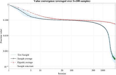
(a) Convergence with no delays between gradient updates

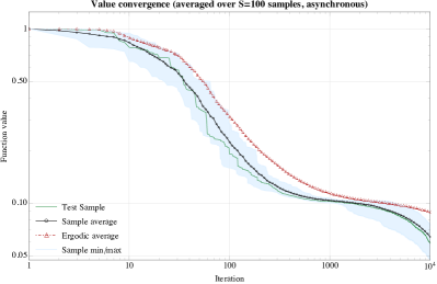
(b) Convergence with linearly growing delays

Figure 3. Value convergence in a non-convex stochastic optimization problem with $d=1001$ degrees of freedom.

For our numerical experiments, we considered a) a synchronous update schedule as a baseline; and b) an asynchronous master-worker framework with random delays that scale as $d_{n}=\Theta(n)$. In both cases, Algorithm 4 was run with a decreasing step-size of the form $\alpha_{n}\propto 1/(n\log n)$ and stochastic gradients drawn from a standard multivariate Gaussian distribution (i.e., zero mean and identity covariance matrix).

Our results are shown in Fig. 3. Starting from a random (but otherwise fixed) initial condition, we ran $S=10^{5}$ realizations of DASGD (with and without delays). We then plotted a randomly chosen trajectory (“test sample” in Fig. 3), the sample average, and the min/max over all samples at every update epoch. For comparison purposes, we also plotted the value of the so-called “ergodic average”

$$\bar{X}_{n}=\frac{\sum_{k=1}^{n}\alpha_{k}X_{k}}{\sum_{k=1}^{n}\alpha_{k}},$$ (21)

which is often used in the analysis of DASGD in the convex case (see e.g., 1). Even though this averaging leads to very robust convergence rate estimates in the convex case, we see here that it performs worse than the worst realization of DASGD. The reason for this is the lack of convexity: due to the ridges and talwegs of the Rosenbrock function, Jensen’s inequality fails dramatically to produce an improvement over $X_{n}$ (and, in fact, causes delays as it causes $X_{n}$ to deviate from its gradient path). Consequently, this simple simulation indicates that establishing convergence of the iterate $X_{n}$ itself is not only theoretically stronger (and hence more difficult) than convergence of the ergodic average, but also more practically relevant.

Appendix A Auxiliary Results

We collect here in one place all the auxiliary results in the existing literature that will be used in our proofs subsequently. The first one is a well-known characterization of convex sets and the projection operator given in [39]:

Lemma A.1.

Let $\mathcal{X}$ be a compact and convex subset of $\mathbb{R}^{d}$. Then for any $x\in\mathcal{X},y\in\mathbb{R}^{d}$:

$$\langle\operatorname{\mathbf{pr}_{\mathcal{X}}}(y)-x,\operatorname{\mathbf{pr}_{\mathcal{X}}}(y)-y\rangle\leq 0.$$ (A.1)

The second one is an $L_{p}$-bounded martingale convergence theorem given in [21]:

Lemma A.2.

Let $S_{n}$ be a martingale adapted to the filtration $\mathcal{S}_{n}$. If for some $p\geq 1$, $\sup_{n\geq 0}\mathbf{E}[|S_{n}|^{p}]<\infty$, then $S_{n}$ converges almost surely to a limiting random variable $S_{\infty}$ with $\mathbf{E}[|S_{\infty}|^{p}]<\infty$.

Remark 6.

Note that $\mathbf{E}[|S_{\infty}|^{p}]<\infty\text{ for }p\geq 1$ obviously implies $S_{\infty}$ is finite almost surely.

The third one is the classical envelope theorem (see [10]).

Lemma A.3.

Let $f:\mathbb{R}^{n}\times\mathbb{R}^{m}\rightarrow\mathbb{R}$ be a continuously differentiable function. Let $U$ be a compact set and consider the problem

$$\max_{x\in U}f(x,\theta).$$ (A.2)

Let $x^{*}:\mathcal{O}\rightarrow\mathbb{R}^{m}$ be a continuous function defined on an open set $\mathcal{O}\subset\mathbb{R}^{m}$ such that for each $\theta\in\mathcal{O}$, $x^{*}(\theta)$ solves the problem in Equation A.2. Define $V:\mathbb{R}^{m}\rightarrow\mathbb{R}$ where $V(\theta)=f(x^{*}(\theta),\theta)$. Then $V(\theta)$ is differentiable on $\mathcal{O}$ and:

$$\operatorname{\nabla}V(\theta)=\operatorname{\nabla}f(x^{*}(\theta),\theta).$$ (A.3)

The fourth one is an elementary sequence result (see [8]).

Lemma A.4.

Let $a_{n},b_{n}$ be two non-negative sequences such that $\sum_{n=1}^{\infty}a_{n}=\infty,\sum_{n=1}^{\infty}a_{n}b_{n}<\infty$. If there exists a real number $K>0$ such that $|b_{n+1}-b_{n}|\leq Ka_{n}$. Then, $\lim_{n\rightarrow\infty}b_{n}=0$.

The fifth one is law of large numbers for martingales given in [21]:

Lemma A.5.

Let $M_{n}=\sum_{k=0}^{n}d_{k}$ be a martingale adapted to $(\mathcal{F}_{n})_{n=0}^{\infty}$ and let $(u_{n})_{n=0}^{\infty}$ be a nondecreasing sequence of positive numbers with $\lim_{n\to\infty}u_{n}=\infty$. If $\sum_{n=0}^{\infty}u_{n}^{-p}\operatorname{\mathbb{E}}[\lvert d_{k}\rvert^{p}\nonscript\>|\nonscript\>\mathopen{}\mathcal{F}_{n}]<\infty$ for some $p\in[1,2]$ (a.s.), then:

$$\lim_{n\to\infty}\frac{M_{n}}{u_{n}}=0\quad\textup{(}a.s.\textup{)}$$ (A.4)

Finally, we recall the standard notion of semiflow.

Definition 3.

A semiflow $P$ on a metric space $(M,d)$ is a continuous map $P:\mathbb{R}_{+}\times M\to M$:

$$(t,x)\to P_{t}(x),$$

such that the semi-group properties hold: $P_{0}$ = identity, $P_{t+s}=P_{t}\circ P_{s}$ for all $(t,s)\in\mathbb{R}_{+}\times\mathbb{R}_{+}$.

Remark 7.

A standard way to induce a semiflow is via an ODE. Specifically, if $F:\mathbb{R}^{m}\to\mathbb{R}^{m}$ is a continuous function and if the following ODE has a unique solution trajectory for each initial point $\tilde{x}\in\mathbb{R}^{m}$:

$$\frac{dx}{dt}= F(x),$$

$$x(0) =\tilde{x},$$

then $P_{t}(\tilde{x})$ defined by the solution trajectory $x(t)\in\mathbb{R}^{m}$ as follows is a semiflow: $P_{t}(\tilde{x})\triangleq x(t)$ with $x(0)=\tilde{x}$. We say $P$ defined in this way is the semiflow induced by the corresponding ODE.

Appendix B Technical Proofs

B.1. General Nonconvex Objectives

B.1.1. Proof of Lemma 1

Proof: We start by rewriting the delayed gradient update $X_{n+1}=X_{n}-\alpha_{n+1}\nabla F(X_{s(n)},\omega_{n+1})$ in Algorithm 3 in two forms as follows, both of which will be used subsequently:

$$\begin{split}&X_{n+1}=X_{n}-\alpha_{n+1}\Bigg{(}\operatorname{\nabla}f(X_{s(n)})+\operatorname{\nabla}F(X_{s(n)},\omega_{n+1})-\operatorname{\nabla}f(X_{s(n)})\Bigg{)}\\ &=X_{n}-\alpha_{n+1}\Bigg{(}\operatorname{\nabla}f(X_{n})+\operatorname{\nabla}f(X_{s(n)})-\operatorname{\nabla}f(X_{n})+\operatorname{\nabla}F(X_{s(n)},\omega_{n+1})-\operatorname{\nabla}f(X_{s(n)})\Bigg{)}.\end{split}$$ (B.1)

Denoted $B\triangleq\sup_{x\in\mathcal{X}}\operatorname{\mathbb{E}}[\|\nabla F(x,\omega)\|_{2}^{2}]$ per Assumption 1. Since $\operatorname{\nabla}f(x)=\operatorname{\mathbb{E}}[\operatorname{\nabla}F(x,\omega)]$ is Lipschitz per Assumption 1, letting $L$ be the Lipschitz constant, we have:

$$\begin{split}&f(X_{n+1})-f(X_{n})\leq\langle\operatorname{\nabla}f(X_{n}),X_{n+1}-X_{n}\rangle+\frac{L}{2}\|X_{n+1}-X_{n}\|_{2}^{2}\\ &=-\alpha_{n+1}\langle\operatorname{\nabla}f(X_{n}),\nabla F(X_{s(n)},\omega_{n+1})\rangle+\frac{L}{2}\|\alpha_{n+1}\nabla F(X_{s(n)},\omega_{n+1})\|_{2}^{2}\\ &=-\alpha_{n+1}\langle\operatorname{\nabla}f(X_{n}),\operatorname{\nabla}f(X_{n})+\operatorname{\nabla}f(X_{s(n)})-\operatorname{\nabla}f(X_{n})+\operatorname{\nabla}F(X_{s(n)},\omega_{n+1})-\operatorname{\nabla}f(X_{s(n)})\rangle\\ &+\frac{L}{2}\alpha_{n+1}^{2}\|\operatorname{\nabla}f(X_{s(n)})+\operatorname{\nabla}F(X_{s(n)},\omega_{n+1})-\operatorname{\nabla}f(X_{s(n)})\|_{2}^{2}\\ &=-\alpha_{n+1}\|\operatorname{\nabla}f(X_{n})\|_{2}^{2}-\alpha_{n+1}\langle\operatorname{\nabla}f(X_{n}),\operatorname{\nabla}f(X_{s(n)})-\operatorname{\nabla}f(X_{n})\rangle\\ &-\alpha_{n+1}\langle\operatorname{\nabla}f(X_{n}),\operatorname{\nabla}F(X_{s(n)},\omega_{n+1})-\operatorname{\nabla}f(X_{s(n)})\rangle\\ &+\frac{L}{2}\alpha_{n+1}^{2}\|\operatorname{\nabla}f(X_{s(n)})+\operatorname{\nabla}F(X_{s(n)},\omega_{n+1})-\operatorname{\nabla}f(X_{s(n)})\|_{2}^{2}\\ &\leq-\alpha_{n+1}\|\operatorname{\nabla}f(X_{n})\|_{2}^{2}+\alpha_{n+1}\|\operatorname{\nabla}f(X_{n})\|_{2}\|\operatorname{\nabla}f(X_{s(n)})-\operatorname{\nabla}f(X_{n})\|_{2}\\ &-\alpha_{n+1}\langle\operatorname{\nabla}f(X_{n}),\operatorname{\nabla}F(X_{s(n)},\omega_{n+1})-\operatorname{\nabla}f(X_{s(n)})\rangle\\ &+\frac{L}{2}\alpha_{n+1}^{2}\Big{\{}2\|\operatorname{\nabla}f(X_{s(n)})\|_{2}^{2}+2\|\operatorname{\nabla}F(X_{s(n)},\omega_{n+1})-\operatorname{\nabla}f(X_{s(n)})\|_{2}^{2}\Big{\}}\\ &\leq-\alpha_{n+1}\|\operatorname{\nabla}f(X_{n})\|_{2}^{2}+\sqrt{B}\alpha_{n+1}\|\operatorname{\nabla}f(X_{s(n)})-\operatorname{\nabla}f(X_{n})\|_{2}\\ &-\alpha_{n+1}\langle\operatorname{\nabla}f(X_{n}),\operatorname{\nabla}F(X_{s(n)},\omega_{n+1})-\operatorname{\nabla}f(X_{s(n)})\rangle\\ &\leq L\alpha_{n+1}^{2}\Big{\{}\sqrt{B}+\|\operatorname{\nabla}F(X_{s(n)},\omega_{n+1})-\operatorname{\nabla}f(X_{s(n)})\|_{2}^{2}\Big{\}},\\ \end{split}$$

where in the last inequality follows because by Jensen’s inequality, we have:

$$\|\operatorname{\nabla}f(X_{n})\|_{2}^{2}\leq\sup_{x\in\mathcal{X}}\|\operatorname{\mathbb{E}}[\nabla F(x,\omega)]\|_{2}^{2}\leq\sup_{x\in\mathcal{X}}\operatorname{\mathbb{E}}[\|\nabla F(x,\omega)\|_{2}^{2}]\leq B.$$

Denote the filtration generated by $X_{0},X_{1},\dots,X_{n}$ to be $\mathcal{F}_{n}$. We take the expectation of both sides of Equation (B.1.1) and obtain:

$$\begin{split}&\operatorname{\mathbb{E}}[f(X_{n+1})-f(X_{n})]\leq-\alpha_{n+1}\operatorname{\mathbb{E}}[\|\operatorname{\nabla}f(X_{n})\|_{2}^{2}]+\sqrt{B}\alpha_{n+1}\operatorname{\mathbb{E}}[\|\operatorname{\nabla}f(X_{s(n)})-\operatorname{\nabla}f(X_{n})\|_{2}]\\ &-\alpha_{n+1}\operatorname{\mathbb{E}}[\langle\operatorname{\nabla}f(X_{n}),\operatorname{\nabla}F(X_{s(n)},\omega_{n+1})-\operatorname{\nabla}f(X_{s(n)})\rangle]+L\sqrt{B}\alpha_{n+1}^{2}\\ &+L\alpha_{n+1}^{2}\operatorname{\mathbb{E}}[\|\operatorname{\nabla}F(X_{s(n)},\omega_{n+1})-\operatorname{\nabla}f(X_{s(n)})\|_{2}^{2}]\\ &=-\alpha_{n+1}\operatorname{\mathbb{E}}[\|\operatorname{\nabla}f(X_{n})\|_{2}^{2}]+\sqrt{B}\alpha_{n+1}\operatorname{\mathbb{E}}[\|\operatorname{\nabla}f(X_{s(n)})-\operatorname{\nabla}f(X_{n})\|_{2}]\\ &-\alpha_{n+1}\operatorname{\mathbb{E}}\Bigg{\{}\operatorname{\mathbb{E}}\Big{\{}\langle\operatorname{\nabla}f(X_{n}),\operatorname{\nabla}F(X_{s(n)},\omega_{n+1})-\operatorname{\nabla}f(X_{s(n)})\rangle\Big{|}\mathcal{F}_{n}\Big{\}}\Bigg{\}}\\ &+L\sqrt{B}\alpha_{n+1}^{2}+L\alpha_{n+1}^{2}\operatorname{\mathbb{E}}[\|\operatorname{\nabla}F(X_{s(n)},\omega_{n+1})-\operatorname{\nabla}f(X_{s(n)})\|_{2}^{2}]\\ &=-\alpha_{n+1}\operatorname{\mathbb{E}}[\|\operatorname{\nabla}f(X_{n})\|_{2}^{2}]+\sqrt{B}\alpha_{n+1}\operatorname{\mathbb{E}}[\|\operatorname{\nabla}f(X_{s(n)})-\operatorname{\nabla}f(X_{n})\|_{2}]\\ &-\alpha_{n+1}\operatorname{\mathbb{E}}\Bigg{\{}\langle\operatorname{\nabla}f(X_{n}),\operatorname{\mathbb{E}}\Big{\{}\operatorname{\nabla}F(X_{s(n)},\omega_{n+1})-\operatorname{\nabla}f(X_{s(n)})\Big{|}\mathcal{F}_{n}\Big{\}}\rangle\Bigg{\}}\\ &+L\sqrt{B}\alpha_{n+1}^{2}+L\alpha_{n+1}^{2}\operatorname{\mathbb{E}}[\|\operatorname{\nabla}F(X_{s(n)},\omega_{n+1})-\operatorname{\nabla}f(X_{s(n)})\|_{2}^{2}]\\ &=-\alpha_{n+1}\operatorname{\mathbb{E}}[\|\operatorname{\nabla}f(X_{n})\|_{2}^{2}]+\sqrt{B}\alpha_{n+1}\operatorname{\mathbb{E}}[\|\operatorname{\nabla}f(X_{s(n)})-\operatorname{\nabla}f(X_{n})\|_{2}]+L\sqrt{B}\alpha_{n+1}^{2}\\ &+L\alpha_{n+1}^{2}\operatorname{\mathbb{E}}[\|\operatorname{\nabla}F(X_{s(n)},\omega_{n+1})-\operatorname{\nabla}f(X_{s(n)})\|_{2}^{2}]\\ &\leq-\alpha_{n+1}\operatorname{\mathbb{E}}[\|\operatorname{\nabla}f(X_{n})\|_{2}^{2}]+\sqrt{B}\alpha_{n+1}\operatorname{\mathbb{E}}[\|\operatorname{\nabla}f(X_{s(n)})-\operatorname{\nabla}f(X_{n})\|_{2}]+L\sqrt{B}\alpha_{n+1}^{2}+4LB\alpha_{n+1}^{2},\\ \end{split}$$

where the third equality follows from $\operatorname{\mathbb{E}}\Big{\{}\operatorname{\nabla}F(X_{s(n)},\omega_{n+1})-\operatorname{\nabla}f(X_{s(n)})\Big{|}\mathcal{F}_{n}\Big{\}}=0$, since $\omega_{n+1}$ is independent of $\mathcal{F}_{n}$, and the last inequality follows from $\operatorname{\mathbb{E}}[\|\operatorname{\nabla}F(X_{s(n)},\omega_{n+1})-\operatorname{\nabla}f(X_{s(n)})\|_{2}^{2}]\leq\sup_{x\in\mathcal{X}}\operatorname{\mathbb{E}}[\|\operatorname{\nabla}F(x,\omega_{n+1})-\operatorname{\nabla}f(x)\|_{2}^{2}]\leq 4B$. Since $\operatorname{\nabla}f$ is $L$-Liptchiz continuous, we have:

$$\|\operatorname{\nabla}f(X_{s(n)})-\operatorname{\nabla}f(X_{n})\|_{2}\leq L\|X_{s(n)}-X_{n}\|_{2}$$

$$=L\Big{\|}X_{s(n)}-X_{{s(n)}+1}+X_{{s(n)}+1}-X_{{s(n)}+2}+\dots+X_{n-1}-X_{n}\Big{\|}_{2}$$

$$=L\Big{\|}\sum_{r=s(n)}^{n-1}\Big{\{}X_{r}-X_{r+1}\Big{\}}\Big{\|}_{2}=L\Big{\|}\sum_{r=s(n)}^{n-1}\alpha_{r+1}\nabla F(X_{s(r)},\omega_{r+1})\Big{\|}_{2}\leq L\sum_{r=s(n)}^{n-1}\alpha_{r+1}\Big{\|}\nabla F(X_{s(r)},\omega_{r+1})\Big{\|}_{2}.$$

Taking the expectation of both sides of the above equation then yields:

$$\operatorname{\mathbb{E}}[\|\operatorname{\nabla}f(X_{s(n)})-\operatorname{\nabla}f(X_{n})\|_{2}]\leq L\sum_{r=s(n)}^{n-1}\alpha_{r+1}\operatorname{\mathbb{E}}[\|\nabla F(X_{s(r)},\omega_{r+1})\|_{2}]$$

$$\leq L\sum_{r=s(n)}^{n-1}\alpha_{r+1}\sup_{x\in\mathcal{X}}\operatorname{\mathbb{E}}[\|\nabla F(x,\omega_{r+1})\|_{2}]$$ (B.3)

$$\leq L\bar{B}\sum_{r=s(n)}^{n-1}\alpha_{r+1},$$ (B.4)

where $\bar{B}\triangleq\sup_{x\in\mathcal{X}}\operatorname{\mathbb{E}}[\|\nabla F(x,\omega_{r+1})\|_{2}]<\infty$ per Remark 1. Combining Equation (B.1.1) with Equation (B.1.1) then yields:

$$\begin{split}&\operatorname{\mathbb{E}}[f(X_{n+1})]-\operatorname{\mathbb{E}}[f(X_{n})]\leq-\alpha_{n+1}\operatorname{\mathbb{E}}[\|\operatorname{\nabla}f(X_{n})\|_{2}^{2}]+L\bar{B}\sqrt{B}\alpha_{n+1}\sum_{r=s(n)}^{n-1}\alpha_{r+1}+L\sqrt{B}\alpha_{n+1}^{2}+4LB\alpha_{n+1}^{2}.\\ \end{split}$$ (B.5)

Telescoping Equation (B.5) then yields:

$$\begin{split}&-\infty<\inf_{x\in\mathcal{X}}f(x)-f(X_{0})\leq\operatorname{\mathbb{E}}[f(X_{T+1})]-f(X_{0})=\sum_{n=0}^{T}\Big{\{}\operatorname{\mathbb{E}}[f(X_{n+1})]-\operatorname{\mathbb{E}}[f(X_{n})]\Big{\}}\\ &\leq-\sum_{n=0}^{T}\alpha_{n+1}\operatorname{\mathbb{E}}[\|\operatorname{\nabla}f(X_{n})\|_{2}^{2}]+L\bar{B}\sqrt{B}\sum_{n=0}^{T}\Big{(}\alpha_{n+1}\sum_{r=s(n)}^{n-1}\alpha_{r+1}\Big{)}+(L\sqrt{B}+4LB)\sum_{n=0}^{T}\alpha_{n+1}^{2}.\\ \end{split}$$ (B.6)

Taking $T\to\infty$, the above equation yields:

$$\begin{split}&-\infty<-\sum_{n=0}^{\infty}\alpha_{n+1}\operatorname{\mathbb{E}}[\|\operatorname{\nabla}f(X_{n})\|_{2}^{2}]+L\bar{B}\sqrt{B}\sum_{n=0}^{\infty}\Big{(}\alpha_{n+1}\sum_{r=s(n)}^{n-1}\alpha_{r+1}\Big{)}+(L\sqrt{B}+4LB)\sum_{n=0}^{\infty}\alpha_{n+1}^{2}.\\ \end{split}$$ (B.7)

Note that in all cases in Assumption 2, we have $\sum_{n=0}^{\infty}\alpha_{n+1}^{2}<\infty$. We next proceed to bound $\sum_{n=0}^{\infty}\Big{(}\alpha_{n+1}\sum_{r=s(n)}^{n-1}\alpha_{r+1}\Big{)}$ and show that it is finite in each of the cases in Assumption 2.

1. In the bounded delays case, since $\sup_{n}d_{n}\leq D$, it follows that $s(n)+D\geq n$ and hence:

   $$\begin{split}&\sum_{n=0}^{\infty}\Big{(}\alpha_{n+1}\sum_{r=s(n)}^{n-1}\alpha_{r+1}\Big{)}\leq\sum_{n=0}^{\infty}\Big{(}\alpha_{n+1}\sum_{r=n-1-D}^{n}\alpha_{r+1}\Big{)}\leq(D+1)\sum_{n=0}^{\infty}\Big{(}\alpha_{n+1}\max_{r\in\{n-1-D,\dots,n\}}\alpha_{r+1}\Big{)}\\ &\leq(D+1)\sum_{n=0}^{\infty}\Big{(}\max_{r\in\{n-1-D,\dots,n\}}\alpha_{r+1}\cdot\max_{r\in\{n-1-D,\dots,n\}}\alpha_{r+1}\Big{)}=(D+1)\sum_{n=0}^{\infty}\Big{(}\max_{r\in\{n-1-D,\dots,n\}}\alpha_{r+1}^{2}\Big{)}\\ &\leq(D+1)\sum_{n=0}^{\infty}\Big{(}\sum_{r=n-1-D}^{n}\alpha_{r+1}^{2}\Big{)}\\ &=(D+1)^{2}\sum_{n=0}^{\infty}\alpha_{n+1}^{2}<\infty,\end{split}$$

   where all the terms $\alpha_{r}$ are defined to be $0$ when $r$ drops below $0$.

2. In the sublinearly growing delays case, since $d_{n}=O(n^{p})$, it follows that $s(n)+Ks^{p}(n)\geq n$ for some positive number $K$, which further implies that $s(n)+Ks(n)\geq s(n)+Ks^{p}(n)\geq n$, thereby leading to $s(n)\geq\frac{n}{K+1}$. Consequently, we have:

   $$\begin{split}&\sum_{n=0}^{\infty}\Big{(}\alpha_{n+1}\sum_{r=s(n)}^{n-1}\alpha_{r+1}\Big{)}\leq\sum_{n=0}^{\infty}\Big{(}\frac{1}{n}\sum_{r=s(n)}^{n}\frac{1}{r}\Big{)}\leq\sum_{n=0}^{\infty}\Big{(}\frac{1}{n}\frac{Ks^{p}(n)}{s(n)}\Big{)}=K\sum_{n=0}^{\infty}\frac{1}{n}s^{p-1}(n)\leq K\sum_{n=0}^{\infty}\frac{1}{n}(\frac{n}{K+1})^{p-1}\\ &\leq(K+1)^{-p}\sum_{n=0}^{\infty}n^{p-2}<\infty.\end{split}$$ (B.8)

3. In the linearly growing delays case, since $d_{n}=O(n)$, it follows that $s(n)+Ks(n)\geq n$ for some positive number $K$ and hence again $s(n)\geq\frac{n}{K+1}$. Consequently, we have:

   $$\sum_{n=0}^{\infty}\Big{(}\alpha_{n+1}\sum_{r=s(n)}^{n-1}\alpha_{r+1}\Big{)} \leq\sum_{n=0}^{\infty}\Big{(}\frac{1}{n\log n}\sum_{r=s(n)}^{n}\frac{1}{r\log r}\Big{)}\leq\sum_{n=0}^{\infty}\Big{(}\frac{1}{n\log n}\sum_{r=s(n)}^{s(n)+Ks(n)}\frac{1}{r\log r}\Big{)}$$

   $$\leq\sum_{n=0}^{\infty}\Big{(}\frac{1}{n\log n}\int_{s(n)}^{s(n)+Ks(n)}\frac{1}{r\log r}dr\Big{)}=\sum_{n=0}^{\infty}\Big{(}\frac{1}{n\log n}\log\frac{\log(s(n)+Ks(n))}{\log s(n)}\Big{)}$$

   $$=\sum_{n=0}^{\infty}\Big{(}\frac{1}{n\log n}\log\frac{\log(K+1)+\log s(n)}{\log s(n)}\Big{)}=\sum_{n=0}^{\infty}\Big{(}\frac{1}{n\log n}\log(1+\frac{\log(K+1)}{\log s(n)})\Big{)}$$

   $$\leq\sum_{n=0}^{\infty}\Big{(}\frac{1}{n\log n}\frac{\log(K+1)}{\log s(n)}\Big{)}\leq\sum_{n=0}^{\infty}\Big{(}\frac{1}{n\log n}\frac{\log(K+1)}{\log n-\log(K+1)}$$

   $$\sim\overline{K}\sum_{n=0}^{\infty}\frac{1}{n(\log n)^{2}}<\infty.$$ (B.9)

4. In the polynomially growing delays case, since $d_{n}=O(n^{q})$, it follows that $s(n)+Ks^{q}(n)\geq n$ for some positive number $K$. Note that in this case, $s(n)=\Omega(n^{\frac{1}{2q}})$, because otherwise, $s(n)+Ks^{q}(n)=O(n^{\frac{1}{2q}}+Kn^{\frac{1}{2}})=o(n)$, which is a contradiction. Consequently, we have:

   $$\sum_{n=0}^{\infty}\Big{(}\alpha_{n+1}\sum_{r=s(n)}^{n-1}\alpha_{r+1}\Big{)} \leq\sum_{n=0}^{\infty}\Big{(}\frac{1}{n\log n\log\log n}\sum_{r=s(n)}^{n}\frac{1}{r\log r\log\log r}\Big{)}$$

   $$\leq\sum_{n=0}^{\infty}\Big{(}\frac{1}{n\log n\log\log n}\sum_{r=s(n)}^{s(n)+Ks^{q}(n)}\frac{1}{r\log r\log\log r}\Big{)}$$

   $$\leq\sum_{n=0}^{\infty}\Big{(}\frac{1}{n\log n\log\log n}\int_{s(n)}^{s(n)+Ks^{q}(n)}\frac{1}{r\log r\log\log r}dr\Big{)}$$

   $$\leq\sum_{n=0}^{\infty}\Big{(}\frac{1}{n\log n\log\log n}\log\frac{\log((K+1)\log s(n)+a\log s(n))}{\log\log s(n)}\Big{)}$$

   $$\leq\sum_{n=0}^{\infty}\Big{(}\frac{1}{n\log n\log\log n}\log(1+\frac{\log(K+1+a)}{\log\log s(n)})\Big{)}$$

   $$\leq\sum_{n=0}^{\infty}\Big{(}\frac{1}{n\log n\log\log n}\frac{\log(K+1+a)}{\log\log s(n)}\Big{)}$$

   $$\leq\sum_{n=0}^{\infty}\Big{(}\frac{1}{n\log n\log\log n}\frac{\log(K+1+a)}{\log\log\frac{n^{\frac{1}{2q}}}{K^{\prime}}}\Big{)}$$

   $$\sim\overline{K}\sum_{n=0}^{\infty}\frac{1}{n\log n(\log\log n)^{2}}<\infty.$$ (B.10)

Consequently, in each of the above 4 cases, we have $\sum_{n=0}^{\infty}\Big{(}\alpha_{n+1}\sum_{r=s(n)}^{n-1}\alpha_{r+1}\Big{)}<\infty$. Therefore, Equation (B.7) yields

$$\begin{split}&-\infty<-\sum_{n=0}^{\infty}\alpha_{n+1}\operatorname{\mathbb{E}}[\|\operatorname{\nabla}f(X_{n})\|_{2}^{2}]+L\bar{B}\sqrt{B}\sum_{n=0}^{\infty}\Big{(}\alpha_{n+1}\sum_{r=s(n)}^{n-1}\alpha_{r+1}\Big{)}+(L\sqrt{B}+4LB)\sum_{n=0}^{\infty}\alpha_{n+1}^{2}\\ &\leq-\sum_{n=0}^{\infty}\alpha_{n+1}\operatorname{\mathbb{E}}[\|\operatorname{\nabla}f(X_{n})\|_{2}^{2}]+\overline{C},\\ \end{split}$$ (B.11)

for some finite constant $\overline{C}$. Reversing the above inequality immediately yields the result:

$$\sum_{n=0}^{\infty}\alpha_{n+1}\operatorname{\mathbb{E}}[\|\operatorname{\nabla}f(X_{n})\|_{2}^{2}]<\infty.$$

$\blacksquare$

B.1.2. Proof of Lemma 2

Proof: We first recall a useful fact: for any two vectors $\mathbf{a},\mathbf{b}$ and any finite-dimensional vector norm $\|\cdot\|$,

$$\Big{|}(\|a\|+\|b\|)(\|a\|-\|b\|)\Big{|}\leq\|a+b\|\|a-b\|.$$ (B.12)

Using this fact, we can expect bound the term in question as follows:

$$\bigg{|}\mathbb{E}[\|\nabla f(X_{n+1})\|_{2}^{2}]-\mathbb{E}[\|\nabla f(X_{n})\|_{2}^{2}]\bigg{|}=\Bigg{|}\mathbb{E}\Bigg{[}\bigg{(}\|\nabla f(X_{n+1})\|_{2}+\|\nabla f(X_{n})\|_{2}\bigg{)}\bigg{(}\|\nabla f(X_{n+1})\|_{2}-\|\nabla f(X_{n})\|_{2}\bigg{)}\Bigg{]}\Bigg{|}$$

$$\leq\mathbb{E}\Bigg{[}\bigg{|}\|\nabla f(X_{n+1})\|_{2}+\|\nabla f(X_{n})\|_{2}\bigg{|}\cdot\bigg{|}\|\nabla f(X_{n+1})\|_{2}-\|\nabla f(X_{n})\|_{2}\bigg{|}\Bigg{]}$$

$$\leq\mathbb{E}\Bigg{[}\bigg{\|}\nabla f(X_{n+1})+\nabla f(X_{n})\bigg{\|}_{2}\cdot\bigg{\|}\nabla f(X_{n+1})-\nabla f(X_{n})\bigg{\|}_{2}\Bigg{]}\leq\mathbb{E}\Bigg{[}2\sup_{x\in\mathcal{X}}\|\nabla f(x)\|_{2}\cdot\bigg{\|}\nabla f(X_{n+1})-\nabla f(X_{n})\bigg{\|}_{2}\Bigg{]}$$

$$\leq 2\sqrt{B}\mathbb{E}\Bigg{[}\bigg{\|}\nabla f(X_{n+1})-\nabla f(X_{n})\bigg{\|}_{2}\Bigg{]}\leq 2\sqrt{B}\mathbb{E}\Bigg{[}L\bigg{\|}X_{n+1}-X_{n}\bigg{\|}_{2}\Bigg{]}=2L\sqrt{B}\mathbb{E}\Bigg{[}\bigg{\|}X_{n+1}-X_{n}\bigg{\|}_{2}\Bigg{]}$$

$$=2L\sqrt{B}\mathbb{E}\Bigg{[}\bigg{\|}\alpha_{n+1}\nabla F(X_{s(n)},\omega_{n+1})\bigg{\|}_{2}\Bigg{]}\leq 2L\sqrt{B}\alpha_{n+1}\sup_{x\in\mathcal{X}}\mathbb{E}\Bigg{[}\bigg{\|}\nabla F(x,\omega_{n+1})\bigg{\|}_{2}\Bigg{]}$$

$$=2L\sqrt{B}\alpha_{n+1}\sup_{x\in\mathcal{X}}\mathbb{E}\Bigg{[}\sqrt{\bigg{\|}\nabla F(x,\omega_{n+1})\bigg{\|}_{2}^{2}}\Bigg{]}$$

$$\leq 2L\sqrt{B}\alpha_{n+1}\sup_{x\in\mathcal{X}}\sqrt{\mathbb{E}\Bigg{[}\bigg{\|}\nabla F(x,\omega_{n+1})\bigg{\|}_{2}^{2}\Bigg{]}}$$

$$\leq 2L\sqrt{B}\alpha_{n+1}\sqrt{B}=2LB\alpha_{n+1},$$

where the first inequality is an application of Jensen’s inequality, the second inequality follows from Equation (B.12) the fifth inequality follows from Lipschitz continuity and the second-to-last inequality follows from another application of Jensen’s inequality and that the squre root function is concave. $\blacksquare$

B.2. Variationally Coherent Objectives

We define the following constants that will be handy later:

1. $C_{1}=\sup_{x\in\mathcal{X}}\operatorname{\mathbb{E}}[\lVert\nabla F(x;\omega)\rVert_{2}]$.

2. $C_{2}=\sup_{x\in\mathcal{X}}\operatorname{\mathbb{E}}[\lVert\nabla F(x;\omega)\rVert_{2}^{2}]$.

3. $C_{3}$ is the Lipschitz constant for $\operatorname{\nabla}f(x)(=\operatorname{\mathbb{E}}[\nabla F(x;\omega)]):$

   $$\|\operatorname{\nabla}f(x)-\operatorname{\nabla}f(x^{\prime})\|_{2}\leq C_{3}\|x-x^{\prime}\|_{2}.$$ (B.13)

4. $C_{4}=\sup_{x,x^{\prime}\in\mathcal{X}}\|x-x^{\prime}\|_{2}.$

B.2.1. Proof of Lemma 3

Per the definition of the energy function, we have:

$$\begin{split}&E_{x^{\ast}}(y)-\|\operatorname{\mathbf{pr}_{\mathcal{X}}}(y)-x^{\ast}\|_{2}^{2}=\|x^{\ast}\|^{2}_{2}-\|\operatorname{\mathbf{pr}_{\mathcal{X}}}(y)\|_{2}^{2}+2\langle y,\operatorname{\mathbf{pr}_{\mathcal{X}}}(y)-x^{\ast}\rangle-\Big{\{}\|\operatorname{\mathbf{pr}_{\mathcal{X}}}(y)\|_{2}^{2}-2\langle\operatorname{\mathbf{pr}_{\mathcal{X}}}(y),x^{\ast}\rangle+\|x^{\ast}\|_{2}^{2}\Big{\}}\\ &=-2\|\operatorname{\mathbf{pr}_{\mathcal{X}}}(y)\|_{2}^{2}+2\langle y-\operatorname{\mathbf{pr}_{\mathcal{X}}}(y),\operatorname{\mathbf{pr}_{\mathcal{X}}}(y)-x^{\ast}\rangle+2\langle\operatorname{\mathbf{pr}_{\mathcal{X}}}(y),\operatorname{\mathbf{pr}_{\mathcal{X}}}(y)-x^{\ast}\rangle+2\langle\operatorname{\mathbf{pr}_{\mathcal{X}}}(y),x^{\ast}\rangle\\ &=2\langle y-\operatorname{\mathbf{pr}_{\mathcal{X}}}(y),\operatorname{\mathbf{pr}_{\mathcal{X}}}(y)-x^{\ast}\rangle\geq 0,\end{split}$$ (B.14)

where the last inequality follows from Lemma A.1. Consequently, $E_{x^{\ast}}(y)\geq\|\operatorname{\mathbf{pr}_{\mathcal{X}}}(y)-x^{\ast}\|_{2}^{2}\geq 0$. Taking the infimum over $\mathcal{X}^{\ast}$ yields $E(y)\geq 0$.

Next, we establish that $E(y)=0$ if and only if $\operatorname{\mathbf{pr}_{\mathcal{X}}}(y)\in\mathcal{X}^{\ast}$. The if part is already established in Remark 4. It suffices to show that $E(y)=0$ implies $\operatorname{\mathbf{pr}_{\mathcal{X}}}(y)\in\mathcal{X}^{\ast}$. To see this, observe that if $E_{x^{\ast}}(y)=0$, we must have $\|\operatorname{\mathbf{pr}_{\mathcal{X}}}(y)-x^{\ast}\|_{2}^{2}=0$, therefore implying $\operatorname{\mathbf{pr}_{\mathcal{X}}}(y)=x^{\ast}.$ Since $E_{x^{\ast}}(y)$ is a continuous function of $x^{\ast}$ for each fixed $y$, and since $\mathcal{X}^{\ast}$ is a compact set, $\inf_{x^{\ast}\in\mathcal{X}^{\ast}}E_{x^{\ast}}(y)$ must be achieved by some $z^{*}\in\mathcal{X}^{\ast}$. Namely $E(y)=E_{z^{*}}(y)$. Consequently, by the preceding observation, $E(y)=0$ implies $\operatorname{\mathbf{pr}_{\mathcal{X}}}(y)=z^{*}\in\mathcal{X}^{\ast}$.

For the second statement, suppose on the contrary $E(y_{n})\to 0$ but $\operatorname{\mathbf{pr}_{\mathcal{X}}}(y_{n})$ does not converge to $\mathcal{X}^{\ast}$. Then there must exist a subsequence $n_{k}$ such that $\operatorname{\mathbf{pr}_{\mathcal{X}}}(y_{n_{k}})$ is bounded away from $\mathcal{X}^{\ast}$. Denoting by $\mathcal{N}(\mathcal{X}^{\ast},\epsilon)$ the $\epsilon$-open ball around $\mathcal{X}^{\ast}$ (i.e. $\mathcal{N}(\mathcal{X}^{\ast},\epsilon)\triangleq\{x\in\mathbb{R}^{d}\mid\text{dist}(x,\mathcal{X}^{\ast})<\epsilon\}$). Then for the subsequence $n_{k}$, there must exist some positive $\epsilon$ such that $\operatorname{\mathbf{pr}_{\mathcal{X}}}(y_{n})$ remains in $\mathcal{X}\cap\mathcal{N}^{c}(\mathcal{X}^{\ast},\epsilon)$. Since $\mathcal{X}\cap\mathcal{N}^{c}(\mathcal{X}^{\ast},\epsilon)$ is an intersection of two closed sets, it is itself closed; it is also bounded since $\mathcal{X}$ is bounded: hence it is compact. Further, since for each fixed $x^{\ast}$, $E_{x^{\ast}}(y)$ is a continuous function of $\operatorname{\mathbf{pr}_{\mathcal{X}}}(y)$, $E_{x^{\ast}}(y)$ must achieve the minimum value on the compact set $\mathcal{X}\cap\mathcal{N}^{c}(\mathcal{X}^{\ast},\epsilon)$, where the minimum value $a_{x^{\ast}}$ is positive per the first statement:

$$E_{x^{\ast}}(y)\geq a_{x^{\ast}}>0,\forall\operatorname{\mathbf{pr}_{\mathcal{X}}}(y)\in\mathcal{X}\cap\mathcal{N}^{c}(\mathcal{X}^{\ast},\epsilon),\forall x^{\ast}\in\mathcal{X}^{\ast}$$

Finally, since $E_{x^{\ast}}(y)$ is continuous in $x^{\ast}$, it must achieve the minimum value (over $x^{\ast}$) on the compact set $\mathcal{X}^{\ast}$, where the minimum value $a$ (corresponding to some $E_{x^{\ast}}(y)$) must again be positive:

$$E(y)=\inf_{x^{\ast}\in\mathcal{X}^{\ast}}E_{x^{\ast}}(y)\geq\inf_{x^{\ast}\in\mathcal{X}^{\ast}}a_{x^{\ast}}=a>0.$$

Consequently, $E(y_{n_{k}})\geq a>0$ since $\operatorname{\mathbf{pr}_{\mathcal{X}}}(y_{n_{k}})\in\mathcal{X}\cap\mathcal{N}^{c}(\mathcal{X}^{\ast},\epsilon),\forall k$. However, on this subsequence, the energy function still converges to $0$ by assumption: $E(y_{n_{k}})\to 0$, which immediately yields a contradiction. The claim is hence established. $\blacksquare$

B.2.2. Proof of Lemma 4

We first prove the first claim. By expanding it, we have:

$$\begin{split}&\|\operatorname{\mathbf{pr}_{\mathcal{X}}}(y)-\hat{y}\|_{2}^{2}-\|\operatorname{\mathbf{pr}_{\mathcal{X}}}(\hat{y})-\hat{y}\|_{2}^{2}=\|\operatorname{\mathbf{pr}_{\mathcal{X}}}(y)-y+y-\hat{y}\|_{2}^{2}-\|\operatorname{\mathbf{pr}_{\mathcal{X}}}(\hat{y})-\hat{y}\|_{2}^{2}\\ &=\|y-\hat{y}\|_{2}^{2}+\|\operatorname{\mathbf{pr}_{\mathcal{X}}}(y)-y\|_{2}^{2}+2\langle\operatorname{\mathbf{pr}_{\mathcal{X}}}(y)-y,y-\hat{y}\rangle-\|\operatorname{\mathbf{pr}_{\mathcal{X}}}(\hat{y})-\hat{y}\|_{2}^{2}\\ &=\|y-\hat{y}\|_{2}^{2}-\Big{\{}\|\operatorname{\mathbf{pr}_{\mathcal{X}}}(\hat{y})-\hat{y}\|_{2}^{2}-\|\operatorname{\mathbf{pr}_{\mathcal{X}}}(y)-y\|_{2}^{2}-2\langle y-\operatorname{\mathbf{pr}_{\mathcal{X}}}(y),\hat{y}-y\rangle\Big{\}}.\\ \end{split}$$ (B.15)

Now define the function $f(x,y)=\|x-y\|_{2}^{2}$. It follows easily that the solution to the problem $\max_{x\in\mathcal{X}}\|x-y\|_{2}^{2}$ is $x^{*}(y)=\operatorname{\mathbf{pr}_{\mathcal{X}}}(y)$. Consequently, by Lemma A.3, $V(y)=f(x^{*}(y),y)$ is a differential function in $y$ and its derivative can be computed explicitly as follows:

$$\operatorname{\nabla}V(y)=\operatorname{\nabla}f(x^{\ast}(y),y)=2(y-x^{*}(y))=2(y-\operatorname{\mathbf{pr}_{\mathcal{X}}}(y)).$$ (B.16)

Futher, since for each $x\in\mathcal{X}$, $f(x,y)$ is a convex function in $y$, and taking the maximum preserves convexity, we have $V(y)$ is also a convex function in $y$. This means that

$$V(\hat{y})-V(y)-\langle\operatorname{\nabla}V(y),\hat{y}-y\rangle\geq 0.$$

By Equation (B.16) and that $V(y)=f(x^{*}(y),y)=\|\operatorname{\mathbf{pr}_{\mathcal{X}}}(y)-x\|_{2}^{2}$, the above equation becomes:

$$\|\operatorname{\mathbf{pr}_{\mathcal{X}}}(\hat{y})-\hat{y}\|_{2}^{2}-\|\operatorname{\mathbf{pr}_{\mathcal{X}}}(y)-y\|_{2}^{2}-2\langle y-\operatorname{\mathbf{pr}_{\mathcal{X}}}(y),\hat{y}-y\rangle\geq 0.$$

Consequently, Equation (A.2) then immediately yields:

$$\|\operatorname{\mathbf{pr}_{\mathcal{X}}}(y)-\hat{y}\|_{2}^{2}-\|\operatorname{\mathbf{pr}_{\mathcal{X}}}(\hat{y})-\hat{y}\|_{2}^{2}\leq\|y-\hat{y}\|_{2}^{2}.$$

We now prove the second part. Expanding using the definition of the Lyapunov function (and skipping some tedious algebra in between), we have:

$$E_{x^{\ast}}(y+\Delta)-E_{x^{\ast}}(y) =\|x^{\ast}\|^{2}_{2}-\|\operatorname{\mathbf{pr}_{\mathcal{X}}}(y+\Delta)\|_{2}^{2}+2\langle y+\Delta,\operatorname{\mathbf{pr}_{\mathcal{X}}}(y+\Delta)-x^{\ast}\rangle$$

$$-\Big{\{}\|x^{\ast}\|^{2}_{2}-\|\operatorname{\mathbf{pr}_{\mathcal{X}}}(y)\|_{2}^{2}+2\langle y,\operatorname{\mathbf{pr}_{\mathcal{X}}}(y)-x^{\ast}\rangle\Big{\}}$$

$$=\|\operatorname{\mathbf{pr}_{\mathcal{X}}}(y)\|_{2}^{2}-\|\operatorname{\mathbf{pr}_{\mathcal{X}}}(y+\Delta)\|_{2}^{2}-2\langle y,\operatorname{\mathbf{pr}_{\mathcal{X}}}(y)-x^{\ast}\rangle+2\langle y+\Delta,\operatorname{\mathbf{pr}_{\mathcal{X}}}(y+\Delta)-x^{\ast}\rangle$$

$$=\|\operatorname{\mathbf{pr}_{\mathcal{X}}}(y)\|_{2}^{2}-\|\operatorname{\mathbf{pr}_{\mathcal{X}}}(y+\Delta)\|_{2}^{2}+2\langle y,\operatorname{\mathbf{pr}_{\mathcal{X}}}(y+\Delta)-\operatorname{\mathbf{pr}_{\mathcal{X}}}(y)\rangle$$

$$\hfill+2\langle\Delta,\operatorname{\mathbf{pr}_{\mathcal{X}}}(y)-x^{\ast}+\operatorname{\mathbf{pr}_{\mathcal{X}}}(y+\Delta)-\operatorname{\mathbf{pr}_{\mathcal{X}}}(y)\rangle$$

$$=2\langle\Delta,\operatorname{\mathbf{pr}_{\mathcal{X}}}(y)-x^{\ast}\rangle+2\langle y+\Delta,\operatorname{\mathbf{pr}_{\mathcal{X}}}(y+\Delta)-\operatorname{\mathbf{pr}_{\mathcal{X}}}(y)\rangle+\|\operatorname{\mathbf{pr}_{\mathcal{X}}}(y)\|_{2}^{2}-\|\operatorname{\mathbf{pr}_{\mathcal{X}}}(y+\Delta)\|_{2}^{2}$$

$$=2\langle\Delta,\operatorname{\mathbf{pr}_{\mathcal{X}}}(y)-x^{\ast}\rangle+\|\operatorname{\mathbf{pr}_{\mathcal{X}}}(y)-(y+\Delta)\|_{2}^{2}-\|\operatorname{\mathbf{pr}_{\mathcal{X}}}(y+\Delta)-(y+\Delta)\|_{2}^{2}$$

$$\leq 2\langle\Delta,\operatorname{\mathbf{pr}_{\mathcal{X}}}(y)-x^{\ast}\rangle+\|\Delta\|_{2}^{2}$$ (B.17)

where the last equality follows from completing the squares and the last inequality follows from the first part of the lemma. $\blacksquare$

B.2.3. Proof of Proposition 1

We provide the details for all the steps.

1. Defining $b_{n}=\operatorname{\nabla}f(x_{s(n)})-\operatorname{\nabla}f(x_{n})$, we can rewrite the gradient update in DAGD as:

   $$y_{n+1} =y_{n}-\alpha_{n+1}\operatorname{\nabla}f(x_{s(n)})$$

   $$=y_{n}-\alpha_{n+1}\operatorname{\nabla}f(x_{n})-\alpha_{n+1}\{\operatorname{\nabla}f(x_{s(n)})-\operatorname{\nabla}f(x_{n})\}$$

   $$=y_{n}-\alpha_{n+1}(\operatorname{\nabla}f(x_{n})+b_{n}).$$ (B.18)

   Recall here once again that $s(n)$ denotes the previous iteration count whose gradient becomes available only at the current iteration $n$. To establish the claim, we start by expanding $b_{n}$ as follows:

   $$\|b_{n}\|_{2} =\|\operatorname{\nabla}f(x_{s(n)})-\operatorname{\nabla}f(x_{n})\|_{2}\leq C_{3}\|x_{s(n)}-x_{n}\|_{2}$$

   $$=C_{3}\|\operatorname{\mathbf{pr}_{\mathcal{X}}}(y_{s(n)})-\operatorname{\mathbf{pr}_{\mathcal{X}}}(y_{n})\|_{2}\leq C_{3}\|y_{s(n)}-y_{n}\|_{2}$$

   $$\leq C_{3}\Big{\{}\|y_{s(n)}-y_{{s(n)}+1}\|_{2}+\|y_{{s(n)}+1}-y_{{s(n)}+2}\|_{2}+\dots+\|y_{n-1}-y_{n}\|_{2}\Big{\}}$$

   $$=C_{3}\sum_{r=s(n)}^{n-1}\|\alpha_{r+1}\operatorname{\nabla}f(x_{s(r)})\|_{2}\leq C_{3}\sup_{x\in\mathcal{X}}\|\operatorname{\nabla}f(x)\|_{2}\sum_{r=s(n)}^{n-1}\alpha_{r+1}=C_{3}V_{\max}\sum_{r=s(n)}^{n-1}\alpha_{r+1}.$$ (B.19)

   We now consider two cases, depending on whether the delays are bounded or not.

   1. If $\{\alpha_{n}\}_{n=1}^{\infty}$ and $d_{n}\leq D,\forall n$ satisfy Assumption 2, then $d_{s(n)}=n-s(n)\leq D$. Consequently,

      $$0<\sum_{r=s(n)}^{n-1}\alpha_{r+1}=\sum_{r=s(n)+1}^{n}\alpha_{r}\leq\sum_{r=n-D}^{n}\alpha_{r}\leq D\max_{r\in\{n-D,\dots,n\}}\alpha_{r}\to 0\quad\text{ as $n\to\infty$},$$ (B.20)

      where the limit approaching $0$ follows from $\lim_{n\to\infty}\alpha_{n}=0$, which itself is a consequence of Assumption 2. This implies $\lim_{n\to\infty}C_{3}V_{\max}\sum_{r=s(n)}^{n-1}\alpha_{r+1}=0$ and consequently, $\lim_{n\to\infty}\|b_{n}\|_{2}=0$.

   2. We consider each of the three conditions in turn.

      When $\alpha_{n-1}=\frac{1}{n}$ and $d_{n}=o(n)$, we have $n-s(n)\leq Ko(s(n))$ for some universal constant $K>0$, which means $n\leq s(n)+Ko(s(n))$. Consequently, we have:

      $$0 <\sum_{r=s(n)}^{n-1}\alpha_{r+1}=\sum_{r=s(n)}^{s(n)+Ko(s(n))}\alpha_{r}\leq\int_{s(n)}^{s(n)+Ko(s(n))}\frac{1}{r}dr$$

      $$=\log(s(n)+Ko(s(n)))-\log s(n)=\log\frac{Ko(s(n))+s(n)}{s(n)}\to\log 1=0\quad\text{as $n\to\infty$},$$ (B.21)

      where the last limit follows from $s(n)\to\infty$ as $n\to\infty$ because $n\leq s(n)+Ko(s(n))$.

      When $\alpha_{n-1}=\frac{1}{n\log n}$ and $d_{n}=O(n)$, it is easy to verify (by integration) that this particular choice of sequence satisfies $\sum_{n=1}^{\infty}\alpha_{n}^{2}<\infty,\sum_{n=1}^{\infty}\alpha_{n}=\infty.$ Since $d_{n}=O(n)$, we have $n-s(n)\leq Ks(n)$ for some universal constant $K>0$, which means $n\leq s(n)+Ks(n)$. Consequently, we have:

      $$0 <\sum_{r=s(n)}^{n-1}\alpha_{r+1}=\sum_{r=s(n)}^{s(n)+Ks(n)}\alpha_{r}\leq\int_{s(n)}^{s(n)+Ks(n)}\frac{1}{r\log r}dr$$

      $$=\log\frac{\log(s(n)+Ks(n))}{\log s(n)}=\log\frac{\log(K+1)+\log s(n)}{\log s(n)}\to 0\quad\text{as $n\to\infty$},$$ (B.22)

      where the last limit follows from $s(n)\to\infty$ as $n\to\infty$ because $n\leq s(n)+Ks(n)$.

      When $\alpha_{n-1}=\frac{1}{n\log n\log\log n}$ and $d_{n}=O(n^{a}),a>1$, it is again easy to verify (by integration) that this particular choice of sequence satisfies Assumption 2. Since $d_{n}=O(n^{a})$, we have $n-s(n)\leq Ks(n)^{a}$ for some universal constant $K>0$, which means $n\leq s(n)+Ks(n)^{a}$. Consequently, we have:

      $$0<\sum_{r=s(n)}^{n-1}\alpha_{r+1}=\sum_{r=s(n)}^{s(n)+Ks(n)^{a}}\alpha_{r} \leq\int_{s(n)}^{s(n)+Ks(n)^{a}}\frac{1}{r\log r\log\log r}dr$$

      $$=\log\frac{\log\log(s(n)+Ks(n)^{a})}{\log\log s(n)}$$

      $$\leq\log\frac{\log\log(s(n)^{a}+Ks(n)^{a})}{\log\log s(n)}$$

      $$<\log\frac{\log((K+1)\log s(n)+a\log s(n))}{\log\log s(n)}$$

      $$=\log\frac{\log(K+1+a)+\log\log s(n)}{\log\log s(n)}\to 0\quad\text{as $n\to\infty$},$$ (B.23)

      where the last limit follows from the fact that $s(n)\to\infty$ as $n\to\infty$ (again, because $n\leq s(n)+Ks(n)^{a}$).

2. With the defintion of $b_{n}$, DAGD can be written as:

   $$x_{n} =\operatorname{\mathbf{pr}_{\mathcal{X}}}(y_{n}),$$ (B.24)

   $$y_{n+1} =y_{n}-\alpha_{n+1}(\operatorname{\nabla}f(x_{n})+b_{n}).$$

   To prove the claim, we start by fixing an arbitrary $x^{\ast}\in\mathcal{X}^{\ast}$ and applying Lemma 4 to bound the energy change in a single gradient update as follows:

   $$\begin{split}E_{x^{*}}(y_{n+1})-E_{x^{*}}(y_{n})&\leq 2\langle y_{n+1}-y_{n},\operatorname{\mathbf{pr}_{\mathcal{X}}}(y_{n})-x^{\ast}\rangle+\|y_{n}-y_{n+1}\|_{2}^{2}\\ &=-2\langle\alpha_{n+1}(\operatorname{\nabla}f(x_{n})+b_{n}),x_{n}-x^{*}\rangle+\|y_{n}-y_{n+1}\|_{2}^{2}.\\ \end{split}$$ (B.25)

   Now telescoping the above inequality yields:

   $$E_{x^{*}}(y_{n+1})-E_{x^{*}}(y_{0}) =\sum_{r=0}^{n}\{E_{x^{*}}(y_{r+1})-E_{x^{*}}(y_{r})\}$$

   $$\leq\sum_{r=0}^{n}\{-2\alpha_{r+1}\langle\operatorname{\nabla}f(x_{r})+b_{r},x_{r}-x^{*}\rangle+\alpha_{r+1}^{2}\|\operatorname{\nabla}f(x_{r})+b_{r}\|_{2}^{2}\}$$

   $$\leq-2\sum_{r=0}^{n}\alpha_{r+1}\{\langle\operatorname{\nabla}f(x_{r}),x_{r}-x^{*}\rangle-\|b_{r}\|_{2}\|x_{r}-x^{*}\|_{2}\}+2\sum_{r=0}^{n}\alpha_{r+1}^{2}\{\|\operatorname{\nabla}f(x_{r})\|_{2}^{2}+\|b_{r}\|_{2}^{2}\}$$

   $$\leq-2\sum_{r=0}^{n}\alpha_{r+1}\{\langle\operatorname{\nabla}f(x_{r}),x_{r}-x^{*}\rangle-C_{4}\|b_{r}\|_{2}\}+2\sum_{r=0}^{n}\alpha_{r+1}^{2}\{C_{2}+B\},$$ (B.26)

   where the last inequality follows from the fact that $b_{n}$’s must be bounded (since $\lim_{n\to\infty}\|b_{n}\|_{2}=0$) and hence let $B\triangleq\sup_{n}\|b_{n}\|_{2}$. By Assumption 2, we have $2\sum_{r=0}^{n}\alpha_{r+1}^{2}\{C_{2}+B\}=\overline{B}<\infty$. Now fix any positive number $\epsilon$. Assume for contradiction purposes $x_{n}$ only enters $\mathcal{N}(x^{*},\epsilon)$ a finite number of times and let $t_{1}$ be the last time this occurs. This means that for all $r>t_{1}$, $x_{r}$ is outside the open set $\mathcal{N}(\mathcal{X}^{\ast},\epsilon)$. Therefore, since a continuous function always achieves its minimum on a compact set, we have: $\langle\operatorname{\nabla}f(x_{r}),x_{r}-x^{*}\rangle\geq\min_{x\in\mathcal{X}-\mathcal{N}(\mathcal{X}^{\ast},\epsilon)}\langle\operatorname{\nabla}f(x),x-x^{*}\rangle\triangleq a>0,\forall r>t_{1}$ (note that $a$ depends on $\epsilon$). Further, since $b_{r}\to 0$ as $r\to\infty$, pick $t_{2}$ such that $\|b_{r}\|_{2}<\frac{a}{2C_{4}},\forall r\geq t_{2}$. Denoting $t=\max(t_{1},t_{2})$, we continue the chain of inequalities in Equation (2) below:

   $$\begin{split}-E_{x^{*}}(y_{0})\\ &\leq E_{x^{*}}(y_{n+1})-E_{x^{*}}(y_{0})\leq-2\sum_{r=0}^{t}\alpha_{r+1}\{\langle\operatorname{\nabla}f(x_{r}),x_{r}-x^{*}\rangle-C_{4}\|b_{r}\|_{2}\}\\ &-2\sum_{r=t+1}^{n}\alpha_{r+1}\{\langle\operatorname{\nabla}f(x_{r}),x_{r}-x^{*}\rangle-C_{4}\|b_{r}\|_{2}\}+2\sum_{r=0}^{n}\alpha_{r+1}^{2}\{C_{2}+B\}\\ &\leq-2\sum_{r=0}^{t}\alpha_{r+1}\{\langle\operatorname{\nabla}f(x_{r}),x_{r}-x^{*}\rangle-C_{4}\|b_{r}\|_{2}\}-2\sum_{r=t+1}^{n}\alpha_{r+1}\{a-C_{4}\|b_{r}\|_{2}\}+\overline{B}\\ &\leq 2C_{4}\sum_{r=0}^{t}\alpha_{r+1}|b_{r}\|_{2}+\overline{B}-2\sum_{r=t+1}^{n}\alpha_{r+1}\{a-\frac{a}{2}\}\\ &=\overline{\overline{B}}-a\sum_{r=t+1}^{n}\alpha_{r+1}\to-\infty,\text{ as }n\to\infty\end{split}$$

   where the first inequality follows from the energy function always being positive (Lemma 3), the second-to-last inequality follows from variational coherence and the limit on the last line follows from Assumption 2 and that $\overline{\overline{B}}\triangleq 2C_{4}\sum_{r=0}^{t}\alpha_{r+1}|b_{r}\|_{2}+\overline{B}$ is just some finite constant. This yields an immediate contradiction and the claim is therefore established.

$\blacksquare$

B.2.4. Proof of Theorem 2

Fix a given $\delta>0$. Since $\alpha_{n}\to 0,b_{n}\to 0$ as $n\to\infty$, for any $a>0$, we can pick an $N$ large enough (depending on $\delta$ and $a$) such that $\forall n\geq N$, the following three statements all hold:

$$\begin{split}&2BC_{4}\alpha_{n+1}+2\alpha_{n+1}^{2}(C_{2}+B^{2})\leq\frac{\delta}{2},\\ &C_{4}\|b_{n}\|_{2}\leq\frac{a}{2},\\ &\alpha_{n+1}(C_{2}+B^{2})<\frac{a}{2}.\end{split}$$ (B.27)

We show that under either of the following two (exhaustive) possibilities, if $E(y_{n})$ is less than $\delta$, $E(y_{n+1})$ is less than $\delta$ as well, where $n\geq N$.

1. Case 1: $E(y_{n})<\frac{\delta}{2}$.

2. Case 2: $\frac{\delta}{2}\leq E(y_{n})<\delta$.

Under Case 1, it follows from Equation (B.25):

$$\begin{split}&E_{x^{*}}(y_{n+1})-E_{x^{*}}(y_{n})\leq-2\alpha_{n+1}\langle\operatorname{\nabla}f(x_{n})+b_{n},x_{n}-x^{*}\rangle+\alpha_{n+1}^{2}\|\operatorname{\nabla}f(x_{n})+b_{n}\|_{2}^{2}\\ &\leq-2\alpha_{n+1}\langle b_{n},x_{n}-x^{*}\rangle+\alpha_{n+1}^{2}\|\operatorname{\nabla}f(x_{n})+b_{n}\|_{2}^{2}\\ &\leq 2\alpha_{n+1}\|b_{n}\|_{2}\|x_{n}-x^{*}\|_{2}+2\alpha_{n+1}^{2}(C_{2}+B^{2})\\ &\leq 2BC_{4}\alpha_{n+1}+2\alpha_{n+1}^{2}(C_{2}+B^{2})\leq\frac{\delta}{2},\end{split}$$ (B.28)

where the second inequality follows from variational coherence. Taking the infimum of $x^{\ast}$ over $\mathcal{X}^{\ast}$ then yields: $E(y_{n+1})-E(y_{n})\leq\frac{\delta}{2}.$ This then implies that $E{(x^{*},y_{n+1})}\leq E(x^{*},y_{n})+\frac{\delta}{2}<\delta$.

Under Case 2, Eq. B.25 readily yields:

$$\begin{split}&E_{x^{*}}(y_{n+1})-E_{x^{*}}(y_{n})\leq-2\alpha_{n+1}\langle\operatorname{\nabla}f(x_{n})+b_{n},x_{n}-x^{*}\rangle+\alpha_{n+1}^{2}\|\operatorname{\nabla}f(x_{n})+b_{n}\|_{2}^{2}\\ &=-2\alpha_{n+1}\langle\operatorname{\nabla}f(x_{n}),x_{n}-x^{*}\rangle-2\alpha_{n+1}\langle b_{n},x_{n}-x^{*}\rangle+\alpha_{n+1}^{2}\|\operatorname{\nabla}f(x_{n})+b_{n}\|_{2}^{2}\\ &\leq-2\alpha_{n+1}a+2\alpha_{n+1}\|b_{n}\|_{2}\|x_{n}-x^{*}\|_{2}+2\alpha_{n+1}^{2}(C_{2}+B^{2})\\ &\leq-2\alpha_{n+1}\Big{\{}a-C_{4}\|b_{n}\|_{2}-\alpha_{n+1}(C_{2}+B^{2})\Big{\}}\\ &\leq-2\alpha_{n+1}\Big{\{}a-\frac{a}{2}-\alpha_{n+1}(C_{2}+B^{2})\Big{\}}\\ &=-2\alpha_{n+1}\Big{\{}\frac{a}{2}-\alpha_{n+1}(C_{2}+B^{2})\Big{\}}\\ &<0,\end{split}$$ (B.29)

where the second inequality follows from $\langle\operatorname{\nabla}f(x_{n}),x_{n}-x^{*}\rangle\geq a$ under Case 2. Taking the infimum of $x^{\ast}$ over $\mathcal{X}^{\ast}$ then yields: $E(y_{n+1})\leq E(y_{n}).$ This then implies that $E{(y_{n+1})}\leq E(y_{n})<\frac{\delta}{2}$.

Consequently, putting the above two cases together therefore yields $E{(y_{n+1})}<\delta$. $\blacksquare$

B.2.5. Proof of Proposition 2

Using the definitions introduced in the main text, we rewrite the gradient update in DASGD as:

$$Y_{n+1}=Y_{n}-\alpha_{n+1}\{\operatorname{\nabla}f(X_{n})+B_{n}+U_{n+1}\}.$$ (B.30)

1. To see that $\sum_{r=0}^{n}U_{n+1}$ is a martingale adapted to $Y_{0},Y_{1}\dots,Y_{n+1}$, first note that, by defintion, $B_{n}$ is adapted to $Y_{0},Y_{1}\dots,Y_{n}$ (since $X_{n}$ is a deterministic function of $Y_{n}$) and $Y_{n+1},Y_{n},B_{n}$ together determine $U_{n+1}$. We then check that their first moments are bounded:

   $$\begin{split}&\operatorname{\mathbb{E}}[\|\sum_{r=0}^{n}\|U_{r+1}\|_{2}]\leq\sum_{r=0}^{n}\operatorname{\mathbb{E}}[\|U_{r+1}\|_{2}]=\sum_{r=0}^{n}\operatorname{\mathbb{E}}[\|\nabla F(X_{s(r)},\omega_{r+1})-\operatorname{\nabla}f(X_{s(r)})\|_{2}]\\ &\leq\sum_{r=0}^{n}\Big{\{}\operatorname{\mathbb{E}}[\|\nabla F(X_{s(r)},\omega_{r+1})\|_{2}]+\operatorname{\mathbb{E}}[\|\operatorname{\nabla}f(X_{s(r)})\|_{2}]\Big{\}}\\ &\leq\sum_{r=0}^{n}\Big{\{}\sup_{x\in\mathcal{X}}\operatorname{\mathbb{E}}[\|\nabla F(x,\omega)\|_{2}]+\sup_{x\in\mathcal{X}}\|\operatorname{\nabla}f(x)\|_{2}\Big{\}}\\ &=\sum_{r=0}^{n}\Big{\{}\sup_{x\in\mathcal{X}}\operatorname{\mathbb{E}}[\|\nabla F(x,\omega)\|_{2}]+\sup_{x\in\mathcal{X}}\|\operatorname{\mathbb{E}}[\nabla F(x,\omega)]\|_{2}\Big{\}}\\ &\leq\sum_{r=0}^{n}2\sup_{x\in\mathcal{X}}\operatorname{\mathbb{E}}[\|\nabla F(x,\omega)\|_{2}]=\sum_{r=0}^{n}2C_{1}=2(n+1)C_{1}<\infty,\end{split}$$ (B.31)

   where the last inequality follows from Jensen’s inequality (since $\|\cdot\|_{2}$ is a convex function). Finally, the martingale property holds because: $\operatorname{\mathbb{E}}[\sum_{r=0}^{n}U_{r+1}\mid Y_{1},\dots,Y_{n+1}]=\operatorname{\mathbb{E}}[\nabla F(X_{s(n)},\omega_{n+1})-\operatorname{\nabla}f(X_{s(n)})\mid Y_{1},\dots,Y_{n}]+\sum_{r=0}^{n-1}U_{r+1}=\sum_{r=0}^{n-1}U_{r+1}.$, since $\omega_{n+1}$ is iid. Therefore, $\sum_{r=0}^{n}U_{r+1}$ is a martingale, and $U_{n+1}$ is a martingale difference sequence adapted to $Y_{0},Y_{1}\dots,Y_{n+1}$.

   Next, we show that $\lim_{n\to\infty}\|B_{n}\|_{2}=0,{a.s.}.$ By definition, we can expand $B_{n}$ as follows:

   $$\|B_{n}\|_{2} =\|\operatorname{\nabla}f(X_{s(n)})-\operatorname{\nabla}f(X_{n})\|_{2}\leq C_{3}\|X_{s(n)}-X_{n}\|_{2}=C_{3}\|\operatorname{\mathbf{pr}_{\mathcal{X}}}(Y_{s(n)})-\operatorname{\mathbf{pr}_{\mathcal{X}}}(Y_{n})\|_{2}$$

   $$\leq C_{3}\|Y_{s(n)}-Y_{n}\|_{2}=C_{3}\Big{\|}Y_{s(n)}-Y_{{s(n)}+1}+Y_{{s(n)}+1}-Y_{{s(n)}+2}+\dots+Y_{n-1}-Y_{n}\Big{\|}_{2}$$

   $$=C_{3}\Big{\|}\sum_{r=s(n)}^{n-1}\Big{\{}Y_{r}-Y_{r+1}\Big{\}}\Big{\|}_{2}=C_{3}\Big{\|}\sum_{r=s(n)}^{n-1}\alpha_{r+1}\nabla F(X_{s(r)},\omega_{r+1})\Big{\|}_{2}$$

   $$=C_{3}\Big{\|}\sum_{r=s(n)}^{n-1}\alpha_{r+1}\Big{\{}\operatorname{\nabla}f(X_{s(r)})+\nabla F(X_{s(r)},\omega_{r+1})-\operatorname{\nabla}f(X_{s(r)})\Big{\}}\Big{\|}_{2}$$

   $$=C_{3}\Big{\|}\sum_{r=s(n)}^{n-1}\alpha_{r+1}\operatorname{\nabla}f(X_{s(r)})+\sum_{r=s(n)}^{n-1}\alpha_{r+1}U_{r+1}\Big{\|}_{2}$$

   $$\leq C_{3}\sum_{r=s(n)}^{n-1}\alpha_{r+1}\|\operatorname{\nabla}f(X_{s(r)})\|_{2}+C_{3}\Big{\|}\sum_{r=s(n)}^{n-1}\alpha_{r+1}U_{r+1}\Big{\|}_{2}$$

   $$\leq C_{3}C_{1}\sum_{r=s(n)}^{n-1}\alpha_{r+1}+C_{3}\|\sum_{r=s(n)}^{n-1}\alpha_{r+1}U_{r+1}\|_{2}$$

   $$=C_{3}C_{1}\sum_{r=s(n)}^{n-1}\alpha_{r+1}+C_{3}\|\sum_{r=0}^{n-1}\alpha_{r+1}U_{r+1}-\sum_{r=0}^{s(n)-1}\alpha_{r+1}U_{r+1}\|_{2},$$ (B.32)

   where the first inequality follows from $\operatorname{\nabla}f$ being Liptichz-continuous (Assumption 3) and the second inequality follows from $\operatorname{\mathbf{pr}_{\mathcal{X}}}$ is a non-expansive map.

   By the same analysis as in the deterministic case, the first part of the last line of Equation (1) converges to $0$ (under each one of the conditions on step-size and delays in Assumption 2):

   $$\lim_{n\to\infty}C_{3}C_{1}\sum_{r=s(n)}^{n-1}\alpha_{r+1}=0.$$ (B.33)

   We then analyze the limit of $\|\sum_{r=0}^{n-1}\alpha_{r+1}U_{r+1}-\sum_{r=0}^{s(n)-1}\alpha_{r+1}U_{r+1}\|_{2}$. Define:

   $$M_{n}=\sum_{r=0}^{n-1}\alpha_{r+1}U_{r+1}.$$

   Since $U_{r+1}$’s are martingale differences, $M_{n}$ is a martingale. Further, in each of the three conditions, $\sum_{n=1}^{\infty}\alpha_{n}^{2}<\infty$. This implies that $M_{n}$ is an $L_{2}$-bounded martingale because:

   $$\begin{split}&\sup_{n}\operatorname{\mathbb{E}}[\|M_{n}\|_{2}^{2}]=\sup_{n}\operatorname{\mathbb{E}}[\Big{\|}\sum_{r=0}^{n-1}\alpha_{r+1}U_{r+1}\Big{\|}_{2}^{2}]=\sup_{n}\operatorname{\mathbb{E}}[\langle\sum_{r=0}^{n-1}\alpha_{r+1}U_{r+1},\sum_{r=0}^{n-1}\alpha_{r+1}U_{r+1}\rangle]\\ &=\sup_{n}\operatorname{\mathbb{E}}[\sum_{i,j}\langle\alpha_{i+1}U_{i+1},\alpha_{j+1}U_{j+1}\rangle]=\sup_{n}\sum_{r=0}^{n-1}\operatorname{\mathbb{E}}[\langle\alpha_{r+1}U_{r+1},\alpha_{r+1}U_{r+1}\rangle]\\ &=\sup_{n}\sum_{r=0}^{n-1}\alpha_{r+1}^{2}\operatorname{\mathbb{E}}[\|U_{r+1}\|_{2}^{2}]\leq\sup_{n}4C_{2}\sum_{r=0}^{n-1}\alpha_{r+1}^{2}\leq 4C_{2}\sum_{r=0}^{\infty}\alpha_{r+1}^{2}<\infty,\end{split}$$ (B.34)

   where the last inequality in the second line follows from the martingale property as follows:

   $$\begin{split}&\operatorname{\mathbb{E}}[\langle\alpha_{i+1}U_{i+1},\alpha_{j+1}U_{j+1}\rangle]=\alpha_{i+1}\alpha_{j+1}\operatorname{\mathbb{E}}[\langle U_{i+1},U_{j+1}\rangle]\\ &=\alpha_{i+1}\alpha_{j+1}\operatorname{\mathbb{E}}[\operatorname{\mathbb{E}}[\langle U_{i+1},U_{j+1}\rangle\mid Y_{0},Y_{1},\dots,Y_{i+1}]]\\ &=\alpha_{i+1}\alpha_{j+1}\operatorname{\mathbb{E}}[\langle U_{i+1},\operatorname{\mathbb{E}}[U_{j+1}\mid Y_{0},Y_{1},\dots,Y_{i+1}]\rangle]=\alpha_{i+1}\alpha_{j+1}\operatorname{\mathbb{E}}[\langle U_{i+1},0\rangle]=0,\end{split}$$ (B.35)

   where the second equality follows from the tower property (and without loss of generality, we have assumed $i<j$, the third equality follows from $U_{i+1}$ is adapted to $Y_{0},Y_{1},\dots,Y_{i+1}$ and the second-to-last equality follows from $U_{n+1}$ is a martingale difference. Consequently, all the cross terms in the second line of Equation (B.34) are $0$. Therefore, by Lemma A.2, by taking $p=2$ $\lim_{n\to\infty}M_{n}=M_{\infty},\text{ a.s.}$, where $M_{\infty}$ has finite second-moment. Further, since in all three cases $s(n)\to\infty$ as $n\to\infty$ (because there is at most a polynomial lag between $s(n)$ and $n$), we have $\lim_{n\to\infty}M_{s(n)}=M_{\infty},\text{ a.s.}$. Therefore

   $$\lim_{n\to\infty}\Big{\{}\sum_{r=0}^{n-1}\alpha_{r+1}U_{r+1}-\sum_{r=0}^{s(n)-1}\alpha_{r+1}U_{r+1}\Big{\}}=\lim_{n\to\infty}\Big{\{}M_{n}-M_{s(n)}\Big{\}}=0,\text{ a.s.},$$

   thereby implying:

   $$\lim_{n\to\infty}C_{3}\Big{\|}\sum_{r=0}^{n-1}\alpha_{r+1}U_{r+1}-\sum_{r=0}^{s(n)-1}\alpha_{r+1}U_{r+1}\Big{\|}_{2}=0.$$ (B.36)

   Combining Equation (B.33) and Equation (B.36) yields $\lim_{n\to\infty}\|B_{n}\|_{2}=0,{a.s.}.$

2. The full DASGD update is then:

   $$X_{n}=\operatorname{\mathbf{pr}_{\mathcal{X}}}(Y_{n})$$ (B.37)

   $$Y_{n+1}=Y_{n}-\alpha_{n+1}\{\operatorname{\nabla}f(X_{n})+B_{n}+U_{n+1}\}.$$ (B.38)

   We now bound the one-step change of the energy function $E(\mathcal{X}^{\ast},Y_{n+1})-E(\mathcal{X}^{\ast},Y_{n})$ (which is now a random quantity) and then telescope the differences.

   Pick an arbitrary $x^{\ast}\in\mathcal{X}^{\ast}$ and apply Lemma 4, we have:

   $$\begin{split}&E_{x^{*}}(Y_{n+1})-E_{x^{*}}(Y_{n})\leq-2\alpha_{n+1}\langle\operatorname{\nabla}f(X_{n})+B_{n}+U_{n+1},X_{n}-x^{*}\rangle+\|Y_{n}-Y_{n+1}\|_{2}^{2}\\ &=-2\alpha_{n+1}\langle\operatorname{\nabla}f(X_{n})+B_{n}+U_{n+1},X_{n}-x^{*}\rangle+\alpha_{n+1}^{2}\|\operatorname{\nabla}f(X_{n})+B_{n}+U_{n+1}\|_{2}^{2}\\ &\leq-2\alpha_{n+1}\langle\operatorname{\nabla}f(X_{n})+B_{n}+U_{n+1},X_{n}-x^{*}\rangle+3\alpha_{n+1}^{2}\Big{\{}\|\operatorname{\nabla}f(X_{n})\|_{2}^{2}+\|B_{n}\|_{2}^{2}+\|U_{n+1}\|_{2}^{2}\Big{\}}\\ &\leq-2\alpha_{n+1}\langle\operatorname{\nabla}f(X_{n})+B_{n}+U_{n+1},X_{n}-x^{*}\rangle+3\alpha_{n+1}^{2}\Big{\{}C_{2}+\|B_{n}\|_{2}^{2}+\|U_{n+1}\|_{2}^{2}\Big{\}}.\end{split}$$ (B.39)

   For contradiction purposes assume $X_{n}$ enters $\mathcal{N}(\mathcal{X}^{\ast},\epsilon)$ only a finite number of times with positive probability. By starting the sequence at a later index if necessary, we can without loss of generality $X_{n}$ never enters $\mathcal{N}(x^{*},\epsilon)$ with positive probability. Then on this event (of $X_{n}$ never entering $\mathcal{N}(\mathcal{X}^{\ast},\epsilon)$), we have $\langle\operatorname{\nabla}f(X_{n}),X_{n}-x^{*}\rangle\geq a>0$ as before. Telescoping Equation (B.39) then yields:

   $$\begin{split}&-\infty<-E_{x^{*}}(Y_{0})\leq E_{x^{*}}(Y_{n+1})-E_{x^{*}}(Y_{0})=\sum_{r=0}^{n}\{E_{x^{*}}(Y_{r+1})-E_{x^{*}}(Y_{r})\}\\ &\leq-2\sum_{r=0}^{n}\alpha_{n+1}\langle\operatorname{\nabla}f(X_{n})+B_{n}+U_{n+1},X_{n}-x^{*}\rangle+3\sum_{r=0}^{n}\alpha_{n+1}^{2}\Big{\{}C_{2}+\|B_{n}\|_{2}^{2}+\|U_{n+1}\|_{2}^{2}\Big{\}}\\ &\leq-2\sum_{r=0}^{n}\alpha_{n+1}\Big{\{}a+\langle B_{n}+U_{n+1},X_{n}-x^{*}\rangle\Big{\}}+3\sum_{r=0}^{n}\alpha_{n+1}^{2}\Big{\{}C_{2}+\|B_{n}\|_{2}^{2}+\|U_{n+1}\|_{2}^{2}\Big{\}}\\ &\to-\infty\text{ a.s. }\text{ as }n\to\infty.\end{split}$$ (B.40)

   We justify the last-line limit of Equation (B.40) by looking at each of its components in turn:

   1. Since $\sum_{r=0}^{n}\alpha_{n+1}^{2}<\infty$, and per the previous step, $\lim_{n\to\infty}\|B_{n}\|_{2}^{2}=0,\text{ a.s.}$, we have $3\sum_{r=0}^{\infty}\alpha_{n+1}^{2}\Big{\{}C_{2}+\|B_{n}\|_{2}^{2}\Big{\}}=C,\text{ a.s.}$, for some constant $C<\infty$.

   2. $\sum_{r=0}^{n}\alpha_{n+1}^{2}\|U_{n+1}\|_{2}^{2}$ is submartingale that is $L_{1}$ bounded since:

      $$\begin{split}&\sup_{n}\operatorname{\mathbb{E}}[\sum_{r=0}^{n}\alpha_{n+1}^{2}\|U_{n+1}\|_{2}^{2}]\leq\sup_{n}\sum_{r=0}^{n}\alpha_{n+1}^{2}\operatorname{\mathbb{E}}[\|U_{n+1}\|_{2}^{2}]\leq\sup_{n}\sum_{r=0}^{n}\alpha_{n+1}^{2}\operatorname{\mathbb{E}}[\|U_{n+1}\|_{2}^{2}]\\ &=\sup_{n}\sum_{r=0}^{n}\alpha_{n+1}^{2}\operatorname{\mathbb{E}}[\|\nabla F(X_{s(n)},\omega_{n+1})-\operatorname{\nabla}f(X_{s(n)})\|_{2}^{2}]\\ &\leq 2\sup_{n}\sum_{r=0}^{n}\alpha_{n+1}^{2}\Big{\{}\operatorname{\mathbb{E}}[\|\operatorname{\nabla}F(X_{s(n)},\omega_{n+1})\|_{2}^{2}]+\operatorname{\mathbb{E}}[\|\operatorname{\nabla}f(X_{s(n)})\|_{2}^{2}]\Big{\}}\\ &\leq 2\sup_{n}\sum_{r=0}^{n}\alpha_{n+1}^{2}\Big{\{}\sup_{x\in\mathcal{X}}\operatorname{\mathbb{E}}[\|\operatorname{\nabla}F(x,\omega)\|_{2}^{2}]+\sup_{x\in\mathcal{X}}\|\operatorname{\nabla}f(x)\|_{2}^{2}\Big{\}}\\ &\leq 2\sup_{n}\sum_{r=0}^{n}2C_{2}\alpha_{n+1}^{2}<\infty.\end{split}$$

      Consequently, by martingale convergence theorem (Lemma A.2 by taking $p=1$), $3\sum_{r=0}^{n}\alpha_{n+1}^{2}\|U_{n+1}\|_{2}^{2}\to R,\text{a.s.}$, for some random variable $R$ that is almost surely finite (in fact $\operatorname{\mathbb{E}}[|R|]<\infty$).

   3. Since $\|B_{n}\|_{2}$ converges to $0$ almost surely, its average also converges to $0$ almost surely:

      $$\sum_{n=0}^{\infty}\frac{\alpha_{n+1}\|B_{n}\|_{2}}{\sum_{r=1}^{n}\alpha_{r+1}}=0,\text{ a.s.},$$

      there by implying that

      $$\sum_{n=0}^{\infty}\frac{\alpha_{n+1}\langle B_{n},X_{n}-x^{*}\rangle}{\sum_{r=1}^{n}\alpha_{r+1}}=0,\text{ a.s.},$$

      since $|\langle B_{n},X_{n}-x^{*}\rangle|\leq\|B_{n}\|_{2}\|X_{n}-x^{*}\|_{2}\leq C_{4}\|B_{n}\|_{2}$.

      In addition, $\alpha_{n+1}\langle U_{n+1},X_{n}-x^{*}\rangle$ is a martingale difference that is $L_{2}$ bounded because $\alpha_{n+1}$ is square summable and

      $$\operatorname{\mathbb{E}}[\|\langle U_{n+1},X_{n}-x^{*}\rangle\|_{2}^{2}]\leq\operatorname{\mathbb{E}}[\|U_{n+1}\|_{2}^{2}\|X_{n}-x^{*}\|_{2}^{2}]\leq C_{4}\operatorname{\mathbb{E}}[\|U_{n+1}\|_{2}^{2}]\leq 4C_{4}C_{2}<\infty.$$

      Consequently, by applying Lemma A.5 with $p=2$ and $u_{n}=\sum_{r=1}^{n}\alpha_{r+1}$ (which is not summable), law of large number for martingales therefore implies:

      $$\sum_{n=0}^{\infty}\frac{\alpha_{n+1}\langle U_{n+1},X_{n}-x^{*}\rangle}{\sum_{r=1}^{n}\alpha_{r+1}}=0,\text{ a.s.}$$

      Combining the above two limits, we have

      $$\lim_{n\to\infty}\frac{\sum_{r=0}^{n}\alpha_{n+1}\langle B_{n}+U_{n+1},X_{n}-x^{*}\rangle}{\sum_{r=0}^{n}\alpha_{r+1}}=0,\text{ a.s.}$$

      Consequently, $-\sum_{r=0}^{n}\alpha_{n+1}\Big{\{}a+\langle B_{n}+U_{n+1},X_{n}-x^{*}\rangle\Big{\}}=-\{\sum_{r=0}^{n}\alpha_{n+1}\}\Big{\{}a+\frac{\sum_{r=0}^{n}\alpha_{n+1}\langle B_{n}+U_{n+1},X_{n}-x^{*}\rangle}{\sum_{r=0}^{n}\alpha_{r+1}}\Big{\}}\to-\infty$, as $n\to-\infty$.

B.2.6. Proof of Lemma 5

The first claim follows by computing the derivative of the energy function with respect to time (for notational simplicity, here we just use $y(t)$ to denote $P(t,y))$:

$$\begin{split}&\frac{d}{dt}E_{x^{\ast}}(y(t))=\frac{d}{dt}\Big{\{}\|x^{\ast}\|^{2}_{2}-\|\operatorname{\mathbf{pr}_{\mathcal{X}}}(y(t))\|_{2}^{2}+2\langle y(t),\operatorname{\mathbf{pr}_{\mathcal{X}}}(y(t))-x^{\ast}\rangle\Big{\}}\\ &=\frac{d}{dt}\Big{\{}-\|\operatorname{\mathbf{pr}_{\mathcal{X}}}(y(t))-y(t)\|_{2}^{2}+\|y(t)\|_{2}^{2}+2\langle y(t),-x^{\ast}\rangle\Big{\}}\\ &=2\langle\dot{y}(t),\operatorname{\mathbf{pr}_{\mathcal{X}}}(y(t))-y(t)\rangle+2\langle y(t),\dot{y}(t)\rangle+2\langle\dot{y}(t),-x^{\ast}\rangle\Big{\}}\\ &=-2\langle\operatorname{\nabla}f(x(t)),x(t)-y(t)\rangle-2\langle\operatorname{\nabla}f(x(t)),y(t)\rangle-2\langle\operatorname{\nabla}f(x(t)),-x^{\ast}\rangle\Big{\}}\\ &=-\langle\operatorname{\nabla}f(x(t))\mathopen{},\mathopen{}x(t)-x^{\ast}\rangle\leq 0,\end{split}$$ (B.41)

where the last inequality is strict unless $\operatorname{\mathbf{pr}_{\mathcal{X}}}(y(t))=x(t)=x^{\ast}$. Take the infimum over $x^{\ast}$ then yields the result: in particular, if $\operatorname{\mathbf{pr}_{\mathcal{X}}}(y(t))=x(t)\notin\mathcal{X}^{\ast}$, then $\frac{d}{dt}E_{x^{\ast}}(y(t))\leq-\epsilon<0,\forall x^{\ast}\in\mathcal{X}^{\ast}$, hence yielding the strict part of the inequality. Note also that even though $\operatorname{\mathbf{pr}_{\mathcal{X}}}(y(t))-y(t)$ is not differentiable, $\|\operatorname{\mathbf{pr}_{\mathcal{X}}}(y(t))-y(t)\|_{2}^{2}$ is; and in computing its derivative, we applied the envelope theorem as given in Lemma A.3.

For the second claim, consider all $y$ that satisfy $E(P(t,y))>\frac{\delta}{2}$. Fix any $x^{\ast}\in\mathcal{X}^{\ast}$. By the monotonicity property in the first part of the lemma, it follows that $E_{x^{*}}(P(s,y))>\frac{\delta}{2},\forall 0\leq s\leq t$. Consequently, $P(s,y)$ must be outside some $\epsilon$ neighborhood of $\mathcal{X}^{\ast}$ for $0\leq s\leq t$, for otherwise, $E_{x^{*}}(P(t,y))$ would be $0$ for at least some $x^{\ast}\in\mathcal{X}^{\ast}$, which is a contradiction to $E(P(t,y))>\frac{\delta}{2}$.

This means that there exists some positive constant $a(\delta)$ such that $\forall 0\leq s\leq t,\forall x^{\ast}\in\mathcal{X}^{\ast}$:

$$\frac{d}{ds}E_{x^{\ast}}(P(s,y))=-\langle\operatorname{\nabla}f(x(s))\mathopen{},\mathopen{}x(s)-x^{\ast}\rangle\leq-a(\delta).\quad$$ (B.42)

Consequently, pick $T(\delta)=\frac{\delta}{2a(\delta)}$, Equation (B.42) implies that for any $t>T(\delta)$:

$$E_{x^{\ast}}(P(t,y))\leq E_{x^{\ast}}(P(T(\delta),y))\leq E_{x^{\ast}}(y)-T(\delta)a(\delta)\leq E_{x^{\ast}}(y)-\frac{\delta}{2}.$$ (B.43)

Taking the supremum over $x^{\ast}\in\mathcal{X}^{\ast}$ then yields:

$$E(P(t,y))\leq E(y)-\frac{\delta}{2}.$$ (B.44)

Since Equation (B.44) is true for any $y$, taking $\sup$ over $y$ establishes the claim. $\blacksquare$

B.3. Proof of Lemma 6

First, from previous analysis, we already know that $U_{n+1}$ is a martingale difference sequence with $\sup_{n}\operatorname{\mathbb{E}}[\|U_{n+1}\|_{2}^{2}]<\infty$ and that $\alpha_{n}$ is a square-summable sequence. Recall also $\lim_{n\to\infty}B_{n}=0$ (a.s.). Now, by combining Proposition 4.1 and Proposition 4.2 in Benaïm [3], we obtain the following sufficient condition for APT:

The affine interpolation curve of the iterates generated by the difference equation $Y_{n+1}=Y_{n}-\alpha_{n+1}\{G(X_{n})+U_{n+1}\}$ is an APT for the solution to the ODE $\dot{y}=-G(y)$ if the following three conditions all hold:

1. $G$ is Lipschitz continuous and bounded. .

2. $U_{n+1}$ is a martingale difference sequence with $\sup_{n}\operatorname{\mathbb{E}}[\|U_{n+1}\|_{2}^{p}]<\infty$ and $\sum_{n=0}^{\infty}\alpha_{n+1}^{1+\frac{p}{2}}<\infty$ for some $p>2$.

By using a similar analysis as in Benaïm [3] (which we omit here due to space limitation), we can show that if the following conditions all hold:

1. $G$ is Lipschitz continuous and bounded.

2. $\lim_{n\to\infty}B_{n}=0$ (a.s.).

3. $U_{n+1}$ is a martingale difference sequence with $\sup_{n}\operatorname{\mathbb{E}}[\|U_{n+1}\|_{2}^{p}]<\infty$ and $\sum_{n=0}^{\infty}\alpha_{n+1}^{1+\frac{p}{2}}<\infty$ for some $p>2$,

then, the affine interpolation curve of the iterates generated by the difference equation $Y_{n+1}=Y_{n}-\alpha_{n+1}\{G(X_{n})+B_{n}+U_{n+1}\}$ is an APT for the solution to the ODE $\dot{y}=-G(y)$.

Take $p=2$ and recall $\operatorname{\nabla}f(\operatorname{\mathbf{pr}_{\mathcal{X}}}(\cdot))$ is Lipschitz continuous and bounded. The above list of three conditions are thus all verified, thereby yielding the result.

B.3.1. Proof of Theorem 3

By Proposition 2, $Y_{n}$ will get arbitrarily close to $\mathcal{X}^{\ast}$ infinitely often. It then suffices to show that, after long enough iterations, if $Y_{n}$ ever gets $\epsilon$-close to $\mathcal{X}^{\ast}$, all the ensuing iterates will be $\epsilon$-close to $\mathcal{X}^{\ast}$ almost surely. The way we show this “trapping" property is to use the energy function. Specifically, we consider $E(x^{\ast},A(t))$ and show that no matter how small $\epsilon$ is, for all sufficiently large $t$, if $E(x^{\ast},A(t_{0}))$ is less than $\epsilon$ for some $t_{0}$, then $E(x^{\ast},A(t))<\epsilon,\forall t>t_{0}$. This would then complete the proof because $A(t)$ actually contains all the DASGD iterates, and hence if $E(x^{\ast},A(t))<\epsilon,\forall t>t_{0}$, then $E(x^{\ast},Y_{n})<\epsilon$ for all sufficiently large $n$. Furthermore, since $A(t)$ contains all the iterates, the hypothesis that “ if $E(x^{\ast},A(t_{0}))$ is less than $\epsilon$ for some $t_{0}$" will be satisfied due to Prop 2.

We now flesh out more details of the proof. Fix any $\epsilon>0$. Since $A(t)$ is an asymptotic pseudotrajectory for $P$, we have:

$$\lim_{t\to\infty}\sup_{0\leq h\leq T}\lVert Y(t+h)-P(h,Y(t))\rVert_{2}=0.$$ (B.45)

Consequently, for any $\delta>0$, there exists some $\tau(\delta,T)$ such that $\lVert Y(t+h)-P(h,Y(t))\rVert_{2}<\delta$ for all $t\geq\tau$ and all $h\in[0,T]$. We therefore have the following chain of inequalities:

$$E_{x^{\ast}}(A(t+h))=E_{x^{\ast}}(P(h,A(t))+A(t+h)-P(h,A(t)))$$ (B.46)

$$\leq E_{x^{\ast}}(P(h,A(t)))+\langle A(t+h)-P(h,A(t))\mathopen{},\mathopen{}\operatorname{\mathbf{pr}_{\mathcal{X}}}(P(h,A(t)))-x^{\ast}\rangle+\frac{1}{2}\lVert A(t+h)-P(h,A(t))\rVert_{2}^{2}$$

$$\leq E_{x^{\ast}}(P(h,A(t)))+C_{4}\delta+\frac{1}{2}\delta^{2}=E_{x^{\ast}}(P(h,A(t)))+\frac{\varepsilon}{2},$$ (B.47)

where in the last step we have choosen $\delta$ small enough such that $C_{4}\delta+\frac{1}{2}\delta^{2}=\frac{\varepsilon}{2}$.

Now by Proposition 2, there exists some $\tau_{0}$ such that $E_{x^{\ast}}(A(\tau_{0}))<\frac{\varepsilon}{2}.$ Our goal is to establish that $E_{x^{\ast}}(A(\tau_{0}+h))<\varepsilon$ for all $h\in[0,\infty)$. To that end, partition the $[0,\infty)$ into disjoint time intervals of the form $[(n-1)T_{\varepsilon},nT_{\varepsilon})$ for some appropriate $T_{\varepsilon}$. By Lemma 5, we have:

$$E_{x^{\ast}}(P(h,A(\tau_{0})))\leq E_{x^{\ast}}(P(0,A(\tau_{0})))=E_{x^{\ast}}(A(\tau_{0}))<\frac{\varepsilon}{2}\quad\text{for all $h\geq 0$}.$$ (B.48)

Consequently:

$$E_{x^{\ast}}(A(\tau_{0}+h))<E_{x^{\ast}}(P(h,A(\tau_{0})))+\frac{\varepsilon}{2}<\frac{\varepsilon}{2}+\frac{\varepsilon}{2}=\varepsilon,$$ (B.49)

where the last inequality is a consequence of (B.48).

Now, assume inductively that Eq. B.49 holds for all $h\in[(n-1)T_{\varepsilon},nT_{\varepsilon})$ for some $n\geq 1$. Then, for all $h\in[(n-1)T_{\varepsilon},nT_{\varepsilon})$, we have:

$$E_{x^{\ast}}(A(\tau_{0}+T_{\varepsilon}+h))<E_{x^{\ast}}(P(T_{\varepsilon},A(\tau_{0}+h)))+\frac{\varepsilon}{2}\leq\max\left\{\frac{\varepsilon}{2},E_{x^{\ast}}(A(\tau_{0}+h))-\frac{\varepsilon}{2}\right\}+\frac{\varepsilon}{2}$$

$$\leq\frac{\varepsilon}{2}+\frac{\varepsilon}{2}=\varepsilon.$$ (B.50)

Consequently, Eq. B.49 holds for all $h\in[nT_{\varepsilon},(n+1)T_{\varepsilon})$. This completes the induction. Taking the infimum over $x^{\ast}$ then completes our proof.

References

• Agarwal and Duchi [2011] Agarwal, Alekh, John C Duchi. 2011. Distributed delayed stochastic optimization. J. Shawe-Taylor, R. S. Zemel, P. L. Bartlett, F. Pereira, K. Q. Weinberger, eds., Advances in Neural Information Processing Systems 24. Curran Associates, Inc., 873–881.
• Avron et al. [2015] Avron, Haim, Alex Druinsky, Anshul Gupta. 2015. Revisiting asynchronous linear solvers: Provable convergence rate through randomization. Journal of the ACM (JACM) 62(6) 51.
• Benaïm [1999] Benaïm, Michel. 1999. Dynamics of stochastic approximation algorithms. Jacques Azéma, Michel Émery, Michel Ledoux, Marc Yor, eds., Séminaire de Probabilités XXXIII, Lecture Notes in Mathematics, vol. 1709. Springer Berlin Heidelberg, 1–68.
• Benaïm and Hirsch [1996] Benaïm, Michel, Morris W. Hirsch. 1996. Asymptotic pseudotrajectories and chain recurrent flows, with applications. Journal of Dynamics and Differential Equations 8(1) 141–176.
• Benaïm and Schreiber [2000] Benaïm, Michel, Sebastian J. Schreiber. 2000. Ergodic properties of weak asymptotic pseudotrajectories for semiflows. Journal of Dynamics and Differential Equations 12(3) 579–598.
• Bertsekas and Tsitsiklis [1996] Bertsekas, Dimitri P, John N Tsitsiklis. 1996. Neuro-dynamic programming. Athena Scientific.
• Bertsekas and Tsitsiklis [1997] Bertsekas, Dimitri P., John N. Tsitsiklis. 1997. Parallel and Distributed Computation: Numerical Methods. Athena Scientific.
• Bertsekas [1995] Bertsekas, D.P. 1995. Nonlinear Programming. Athena Scientific. URL https://books.google.com/books?id=QeweAQAAIAAJ.
• Borkar [2008] Borkar, Vivek S. 2008. Stochastic Approximation: A Dynamical Systems Viewpoint. Cambridge University Press and Hindustan Book Agency.
• Carter [2001] Carter, M. 2001. Foundations of Mathematical Economics. MIT Press. URL https://books.google.com/books?id=KysvrGGfzq0C.
• Chaturapruek et al. [2015] Chaturapruek, Sorathan, John C Duchi, Christopher Ré. 2015. Asynchronous stochastic convex optimization: the noise is in the noise and sgd don’t care. Advances in Neural Information Processing Systems. 1531–1539.
• de Souza and Silva [2012] de Souza, P.N., J.N. Silva. 2012. Berkeley Problems in Mathematics. Problem Books in Mathematics, Springer New York. URL https://books.google.com/books?id=cikdswEACAAJ.
• Dean et al. [2012a] Dean, Jeffrey, Greg Corrado, Rajat Monga, Kai Chen, Matthieu Devin, Mark Mao, Andrew Senior, Paul Tucker, Ke Yang, Quoc V Le, et al. 2012a. Large scale distributed deep networks. Advances in neural information processing systems. 1223–1231.
• Dean et al. [2012b] Dean, Jeffrey, Greg S. Corrado, Rajat Monga, Kai Chen, Matthieu Devin, Quoc V. Le, Mark Z. Mao, Marc’Aurelio Ranzato, Andrew Senior, Paul Tucker, Ke Yang, Andrew Y. Ng. 2012b. Large scale distributed deep networks. Proceedings of the 25th International Conference on Neural Information Processing Systems - Volume 1. NIPS’12, Curran Associates Inc., USA, 1223–1231.
• Dey et al. [2017] Dey, Santanu S, Marco Molinaro, Qianyi Wang. 2017. Analysis of sparse cutting planes for sparse milps with applications to stochastic milps. Mathematics of Operations Research .
• Feng et al. [2013] Feng, Jiashi, Huan Xu, Shuicheng Yan. 2013. Online robust pca via stochastic optimization. Advances in Neural Information Processing Systems. 404–412.
• Fercoq and Richtárik [2015] Fercoq, Olivier, Peter Richtárik. 2015. Accelerated, parallel, and proximal coordinate descent. SIAM Journal on Optimization 25(4) 1997–2023.
• Feyzmahdavian et al. [2016] Feyzmahdavian, Hamid Reza, Arda Aytekin, Mikael Johansson. 2016. An asynchronous mini-batch algorithm for regularized stochastic optimization. IEEE Transactions on Automatic Control 61(12) 3740–3754.
• Ge et al. [2015] Ge, Rong, Furong Huang, Chi Jin, Yang Yuan. 2015. Escaping from saddle points?online stochastic gradient for tensor decomposition. Conference on Learning Theory. 797–842.
• Ghadimi and Lan [2013] Ghadimi, Saeed, Guanghui Lan. 2013. Stochastic first-and zeroth-order methods for nonconvex stochastic programming. SIAM Journal on Optimization 23(4) 2341–2368.
• Hall and Heyde [1980] Hall, P., C. C. Heyde. 1980. Martingale Limit Theory and Its Application. Probability and Mathematical Statistics, Academic Press, New York.
• Héliou et al. [2020] Héliou, Amélie, Panayotis Mertikopoulos, Zhengyuan Zhou. 2020. Gradient-free online learning in continuous games with delayed rewards. ICML ’20: Proceedings of the 37th International Conference on Machine Learning.
• Hong [2017] Hong, Mingyi. 2017. A distributed, asynchronous and incremental algorithm for nonconvex optimization: An admm approach. IEEE Transactions on Control of Network Systems .
• Hsieh et al. [2020] Hsieh, Yu-Guan, Franck Iutzeler, Jérôme Malick, Panayotis Mertikopoulos. 2020. Multi-agent online optimization with delays: Asynchronicity, adaptivity, and optimism. https://arxiv.org/abs/2012.11579.
• Jin et al. [2017] Jin, Chi, Rong Ge, Praneeth Netrapalli, Sham M Kakade, Michael I Jordan. 2017. How to escape saddle points efficiently. Proceedings of the 34th International Conference on Machine Learning-Volume 70. JMLR. org, 1724–1732.
• Joulani et al. [2016] Joulani, Pooria, András György, Csaba Szepesvári. 2016. Delay-tolerant online convex optimization: Unified analysis and adaptive-gradient algorithms. AAAI ’16: Proceedings of the 30th Conference on Artificial Intelligence.
• Krizhevsky et al. [2012] Krizhevsky, Alex, Ilya Sutskever, Geoffrey E Hinton. 2012. Imagenet classification with deep convolutional neural networks. F. Pereira, C. J. C. Burges, L. Bottou, K. Q. Weinberger, eds., Advances in Neural Information Processing Systems 25. Curran Associates, Inc., 1097–1105.
• Kushner and Yin [2013] Kushner, H., G.G. Yin. 2013. Stochastic Approximation and Recursive Algorithms and Applications. Stochastic Modelling and Applied Probability, Springer New York. URL https://books.google.com/books?id=sB0GCAAAQBAJ.
• Lee et al. [2016] Lee, Jason D, Max Simchowitz, Michael I Jordan, Benjamin Recht. 2016. Gradient descent converges to minimizers. arXiv preprint arXiv:1602.04915 .
• Lee et al. [2011] Lee, Jinho, John Hasenbein, David Morton. 2011. Stochastic optimization models for rapid detection of viruses in cellphone networks. Tech Report .
• Lian et al. [2015] Lian, Xiangru, Yijun Huang, Yuncheng Li, Ji Liu. 2015. Asynchronous parallel stochastic gradient for nonconvex optimization. Advances in Neural Information Processing Systems. 2737–2745.
• Lian et al. [2016] Lian, Xiangru, Huan Zhang, Cho-Jui Hsieh, Yijun Huang, Ji Liu. 2016. A comprehensive linear speedup analysis for asynchronous stochastic parallel optimization from zeroth-order to first-order. Advances in Neural Information Processing Systems. 3054–3062.
• Liu and Wright [2015] Liu, Ji, Stephen J Wright. 2015. Asynchronous stochastic coordinate descent: Parallelism and convergence properties. SIAM Journal on Optimization 25(1) 351–376.
• Liu et al. [2014] Liu, Ji, Stephen J Wright, Srikrishna Sridhar. 2014. An asynchronous parallel randomized kaczmarz algorithm. arXiv preprint arXiv:1401.4780 .
• Mania et al. [2017] Mania, Horia, Xinghao Pan, Dimitris Papailiopoulos, Benjamin Recht, Kannan Ramchandran, Michael I Jordan. 2017. Perturbed iterate analysis for asynchronous stochastic optimization. SIAM Journal on Optimization 27(4) 2202–2229.
• Marecek et al. [2015] Marecek, Jakub, Peter Richtarik, Martin Takac. 2015. Distributed block coordinate descent for minimizing partially separable functions. Numerical Analysis and Optimization. Springer, 261–288.
• Mertikopoulos et al. [2019] Mertikopoulos, Panayotis, Bruno Lecouat, Houssam Zenati, Chuan-Sheng Foo, Vijay Chandrasekhar, Georgios Piliouras. 2019. Optimistic mirror descent in saddle-point problems: Going the extra (gradient) mile. ICLR ’19: Proceedings of the 2019 International Conference on Learning Representations.
• Mertikopoulos and Zhou [2019] Mertikopoulos, Panayotis, Zhengyuan Zhou. 2019. Learning in games with continuous action sets and unknown payoff functions. Mathematical Programming 173(1-2) 465–507.
• Nesterov [2004] Nesterov, Yurii. 2004. Introductory Lectures on Convex Optimization: A Basic Course. No. 87 in Applied Optimization, Kluwer Academic Publishers.
• Paine et al. [2013] Paine, Thomas, Hailin Jin, Jianchao Yang, Zhe Lin, Thomas Huang. 2013. Gpu asynchronous stochastic gradient descent to speed up neural network training. arXiv preprint arXiv:1312.6186 .
• Quanrud and Khashabi [2015] Quanrud, Kent, Daniel Khashabi. 2015. Online learning with adversarial delays. NIPS ’15: Proceedings of the 29th International Conference on Neural Information Processing Systems.
• Recht et al. [2011] Recht, Benjamin, Christopher Re, Stephen Wright, Feng Niu. 2011. Hogwild: A lock-free approach to parallelizing stochastic gradient descent. Advances in neural information processing systems. 693–701.
• Rosenbrock [1960] Rosenbrock, Howard Harry. 1960. An automatic method for finding the greatest or least value of a function. Computer Journal 3(3) 175–184.
• Ruszczyński and Shapiro [2003] Ruszczyński, Andrzej, Alexander Shapiro. 2003. Stochastic programming models. Handbooks in operations research and management science 10 1–64.
• Shapiro and Philpott [2007] Shapiro, Alexander, Andy Philpott. 2007. A tutorial on stochastic programming .
• Tappenden et al. [2017] Tappenden, Rachael, Martin Takac, Peter Richtarik. 2017. On the complexity of parallel coordinate descent. Optimization Methods and Software 1–24.
• Tran et al. [2015] Tran, Kenneth, Saghar Hosseini, Lin Xiao, Thomas Finley, Mikhail Bilenko. 2015. Scaling up stochastic dual coordinate ascent. Proceedings of the 21th ACM SIGKDD International Conference on Knowledge Discovery and Data Mining. KDD ’15, ACM, New York, NY, USA, 1185–1194.
• Tsitsiklis [1984] Tsitsiklis, John N. 1984. Problems in decentralized decision making and computation. Ph.D. thesis, MIT.
• Tsitsiklis et al. [1986] Tsitsiklis, John N., Dimitri P. Bertsekas, Michael Athans. 1986. Distributed asynchronous deterministic and stochastic gradient optimization algorithms 31(9) 803–812.
• Uryasev and Pardalos [2010] Uryasev, S., P.M. Pardalos. 2010. Stochastic Optimization: Algorithms and Applications. Applied Optimization, Springer US. URL https://books.google.com/books?id=MNL6kQAACAAJ.
• Wang et al. [2016] Wang, Yu-Xiang, Veeranjaneyulu Sadhanala, Wei Dai, Willie Neiswanger, Suvrit Sra, Eric Xing. 2016. Parallel and distributed block-coordinate frank-wolfe algorithms. International Conference on Machine Learning. 1548–1557.
• Wright [2015] Wright, Stephen J. 2015. Coordinate descent algorithms. Mathematical Programming 151(1) 3–34.
• Zhang and Kwok [2014] Zhang, Ruiliang, James Kwok. 2014. Asynchronous distributed admm for consensus optimization. International Conference on Machine Learning. 1701–1709.
• Zhang et al. [2013] Zhang, Shanshan, Ce Zhang, Zhao You, Rong Zheng, Bo Xu. 2013. Asynchronous stochastic gradient descent for dnn training. 2013 IEEE International Conference on Acoustics, Speech and Signal Processing.
• Zhang et al. [2015] Zhang, Sixin, Anna E Choromanska, Yann LeCun. 2015. Deep learning with elastic averaging sgd. Advances in Neural Information Processing Systems. 685–693.
• Zhou et al. [2017] Zhou, Zhengyuan, Panayotis Mertikopoulos, Nicholas Bambos, Stephen Boyd, Peter W Glynn. 2017. Stochastic mirror descent in variationally coherent optimization problems. Advances in Neural Information Processing Systems 30 7040–7049.
• Zhou et al. [2020] Zhou, Zhengyuan, Panayotis Mertikopoulos, Nicholas Bambos, Stephen P. Boyd, Peter W. Glynn. 2020. On the convergence of mirror descent beyond stochastic convex programming. SIAM Journal on Optimization 30(1) 687–716. doi:10.1137/17M1134925.
• Zhou et al. [2018] Zhou, Zhengyuan, Panayotis Mertikopoulos, Nicholas Bambos, Peter Glynn, Yinyu Ye, Li-Jia Li, Li Fei-Fei. 2018. Distributed asynchronous optimization with unbounded delays: How slow can you go? International Conference on Machine Learning. 5970–5979.