Random search in fluid flow aided by chemotaxis

Abstract.

In this paper, we consider the dynamics of a 2D target-searching agent performing Brownian motion under the influence of fluid shear flow and chemical attraction. The analysis is motivated by numerous situations in biology where these effects are present, such as broadcast spawning of marine animals and other reproduction processes or workings of the immune systems. We rigorously characterize the limit of the expected hit time in the large flow amplitude limit as corresponding to the effective one-dimensional problem. We also perform numerical computations to characterize the finer properties of the expected duration of the search. The numerical experiments show many interesting features of the process, and in particular existence of the optimal value of the shear flow that minimizes the expected target hit time and outperforms the large flow limit.

1. Introduction

In this paper, we analyze the agent randomly searching for a target in the ambient shear flow, aided by chemotaxis on the chemical released by the target. This process occurs in multiple settings in biology. One example is reproduction for many species, where eggs secrete chemicals that attracts sperm and help improve fertilization rates. This is especially well studied for marine life such as corals, sea urchins, mollusks, etc (see [16, 25, 26, 31] for further references), but the role of chemotaxis in fertilization extends to a great number of species, including humans [24]. Another process where chemotaxis plays an important role is mammal immune systems fighting bacterial infections. Inflamed tissues release special proteins, called chemokines, that serve to chemically attract monocytes, blood killer cells, to the source of infection [6, 28]. Chemotaxis can also be involved when things go awry, for instance, playing a role in tumor growth [29]. One can also envision future applications to medical mini-robots tasked with finding some sort of targets. These processes take place in fluids, and on the length scales where the ambient fluid motion can be effectively regarded as shear flow.

As a mathematical model, we consider the following stochastic differential equation (SDE) subject to initial condition $\mathbf{X}_{0}=(x_{0},y_{0})$ on the torus $\mathbb{T}^{2}=[0,L)^{2}:$

(1.1i) $$\left(\begin{array}[]{rr}dX_{t}\\ dY_{t}\end{array}\right)= \left(\begin{array}[]{cc}{A}u(Y_{t})\\ 0\end{array}\right)dt+\left(\begin{array}[]{c}V^{(1)}\\ V^{(2)}\end{array}\right)dt+\sqrt{2\nu}\left(\begin{array}[]{rr}dB_{t}^{(1)}\\ dB_{t}^{(2)}\end{array}\right);$$

(1.1j) $$V= (V^{(1)},V^{(2)})=\varphi({\chi}|\nabla c|)\frac{\nabla c}{|\nabla c|},\quad-\Delta c+{A}u(y)\partial_{x}c=n-c.$$

The terms on the right hand side of (1.1i) model advection, chemotaxis, and random motion respectively. The function $c$ is the concentration of the chemical, and $n$ is the density of the target, that will be located in a small area at the center of the torus. For chemotaxis, we choose a variant of flux-limited models that have been studied in, for example, [3, 14, 15, 23]. and which is more realistic than the classical Keller-Segel form in that it places a speed limit on the agent.

The SDE (1.1i) models a single agent’s searching process subject to ambient fluid advection, random Brownian motion, and chemical attraction. The searching is successful if the agent reaches the region occupied by the target population $n$. The agent, positioned at point $\mathbf{X}_{t}=(X_{t},Y_{t})$, is transported by the ambient shear flow $({A}u(Y_{t}),0)$ with magnitude ${A}\in\mathbb{R}_{+}$. Meanwhile, the agent also moves randomly, which is captured by the Brownian motion $\sqrt{\nu}d\mathbf{B}_{t}=\sqrt{\nu}(dB_{t}^{(1)},dB_{t}^{(2)})$ with diffusivity $\nu$. Finally, the agent aggregates towards the higher concentration of chemoattractant density $c$, secreted by the target population $n$. The parameter ${\chi}$ denotes the chemical sensitivity, and the smooth cut-off function $\varphi\in C^{2}(\mathbb{R}_{+})$ enforces finite speed of aggregation. In fact, we will take the function $\varphi$ to be close to piecewise linear, allowing its parametrization with essentially two parameters: the maximum speed and chemical sensitivity. We consider the regime where the chemoattractant density $c$ reaches equilibrium at a much faster time scale than other relevant time scales of the problem, thus the density $c$ satisfies the elliptic equation (1.1j).

Our main goal in this paper is to gain insight into the interaction of the three transport mechanisms present in the model and their cumulative effect on the expected length of the search. There are many works dedicated to interaction of advection and diffusion - see e.g. [10] and [17]; the latter source specifically looks at diffusion exit times and contains further references. However we are not aware of any detailed mathematical - rigorous or numerical - analysis of the problem when chemotaxis is added in the mix. Our work has been largely inspired by biological experiments on broadcast spawning of abalone conducted by Riffell and Zimmer. Marine animals such as abalones, corals, and shrimp release their egg and sperm cells into the ambient ocean. The gametes are positively buoyant and rise to the surface, where fertilization happens. The eggs are not mobile but release attractive pheromone. The sperms aggregate towards the eggs by a combination of random motion and chemotaxis-guided transport. Since the processes occurs in a fluid flow that is effectively shear on length scales involved, it is of biological interest to study the relation of fertilization success rate, chemotaxis, and shear flow speed. In the papers [25], [26], [31], Zimmer, Riffell and their research group put well-mixed abalone sperms and eggs in a Taylor-Couette tank and study the quantitative relationships. The positive effect of chemotaxis has been clearly established; as far as the shear flow, the researchers observed that its effect is two-fold. If the shear rate is moderately slow, the shear enhanced fertilization. On the other hand, if the shear rate is faster than a certain threshold, the fertilization rate starts declining. We notice that the sperms are evenly distributed in the seawater in the biological experiment, and the experimental time is limited ($\approx 15$ seconds). Hence only the group of sperms surrounding the eggs have access to the egg zone. As a result, the microflow environment play a dominant role during the fertilization process under this setup. Our model addresses a related but different situation where there is a single searcher and, instead of the fertilization success rate (percentage of fertilized eggs), it monitors expected search time. We consider this set up since we would like to represent the problem in the most fundamental form, and to understand the role of different forces affecting the search on this fundamental level. Nevertheless, in our numerical computations, we mostly focus on the parameter regimes relevant for the experiments of Riffell and Zimmer.

Our main results are as follows. On the rigorous level, we are able to establish that the very large shear rates are a dimension reduction mechanism: the expected search time converges to the one of the corresponding one-dimensional problem with effective 1D chemotaxis. Such result is not unexpected, and is similar to the findings of Freidlin-Wentzel theory [10]. The presence of chemotaxis, however, necessitates some novel elements in the analysis. Numerically, we observe several phenomena that we find interesting. First, we see quite fast decrease of the expected hitting time already for quite small values of shear and chemotactic coupling. Second, we discover that in the context of our model, there is an optimal shear rate range where the searching time is minimal, and is less than the limiting 1D large shear searching time. This is entirely due to presence of chemotaxis; when it is absent, the expected hitting time is monotone decaying in flow amplitude. This finding agrees with the results of biological experiments. The difference is that in the experiments the fertilization rate declines much more steeply (and probably towards zero) for large shears. This effect is likely not because sperm have trouble finding eggs, but rather due to their inability to stay around for time necessary for fertilization. In our set up, there is no such mechanism: we just register the hit. Nevertheless, even on the fundamental level of random search/chemotaxis/fluid flow interaction, we observe the non-trivial phenomena of optimal shear range. The third interesting effect we find in the framework of our model and within the range of parameters that we tested is that increasing chemical sensitivity appears meaningfully more important for improving search performance than increasing the maximal speed. We believe that these observations can be useful for better understanding of biological processes that may involve additional elements and factors, but include the interaction of the three basic forces that we study here. We note that numerical experiments on random search in a shear flow (without chemotaxis) were also carried out in [4].

The paper is organized as follows: in the next section, we introduce the general set up and key parameters of the model in more detail and present our numerical scheme. We then proceed to describe the results of the numerical experiments. After this we state the rigorous results that we are able to prove, and proceed with the proofs.

2. General Set Up and Numerical Scheme

2.1. The set up and first hitting time

Recall that in this paper we focus on the searching success of an individual agent, whose initial position may be relatively distant from the target zone. We focus on the following geometric configuration in our numerical and analytic exploration. The domain $(L{\mathbb{T}})^{2}$ has dimension $[0,L)^{2}$. The chemical cutoff function $\varphi(\cdot)\in C^{\infty}([0,\infty))$ is chosen so that $\varphi(0)=0$ and $\varphi^{\prime}(0)=1$, $\varphi$ is monotone increasing, and $\lim_{r\rightarrow\infty}\varphi(r)=||\varphi||_{\infty}<\infty$ (see Figure 2). The norm $||\varphi||_{\infty}$ has the meaning of the maximal chemical-induced speed of the agent. The target density $n$ is stationary and concentrated in the target zone $E_{\delta}$, which is a disk $B((\frac{L}{2},\frac{L}{2});\delta)$. The size of the target $\delta$ is much smaller than $L$. The total mass of the target density is $||n||_{L^{1}({\mathbb{T}}^{2})}$ is normalized to be equal to one. The searching starts at a point $(x_{0},y_{0})$. In our numerics, the agent starts at point $(0,0)$, which is a distance $\frac{L}{\sqrt{2}}$ away from the target zone. We tried other starting positions with very similar qualitative results. The shear profile is adapted to the size of the torus and is given by $u(y)=\sin\left(\frac{2\pi(y-L/2)}{L}\right),$ with coupling constant $A$. We simulated a few other shear flow profiles, but did not observe a significant difference as long as the shear rate near the egg zone is the same. Therefore, we restrict ourselves to the $A\sin\left(\frac{2\pi(y-L/2)}{L}\right)$-flow for the sake of simplicity. In Figure 1, we provide a diagram with the general setup.

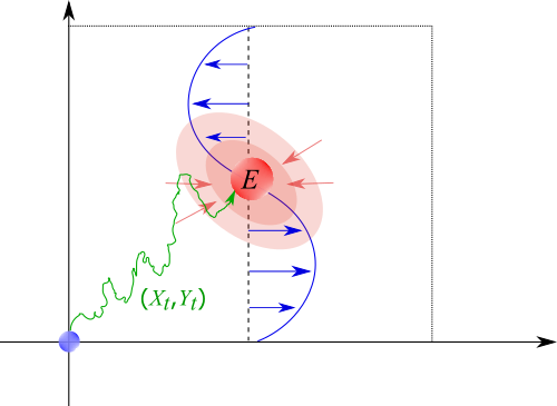
Figure 1. Problem setup.

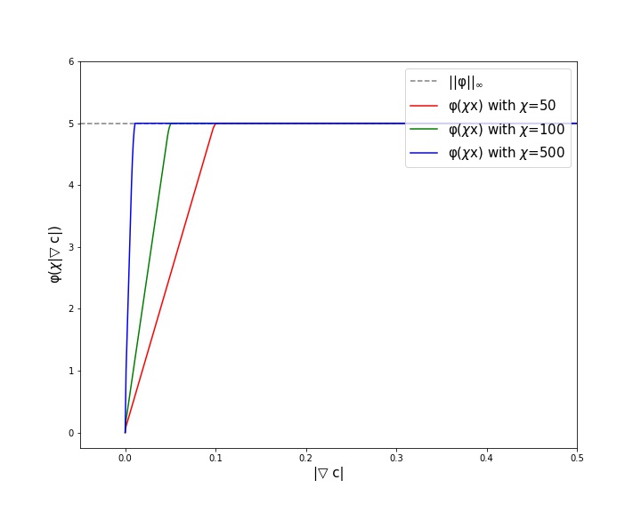
Figure 2. Cutoff function $\varphi(x)$ for chemotaxis.

To quantify the success of the search, we consider the expectation of the first hitting time of the target zone, i.e.

(2.1) $$T^{(x_{0},y_{0})}(\omega)=\min\{\tau|\mathbf{X}_{\tau}(\omega)\in E_{\delta}=B((L/2,L/2);\delta)\}.$$

Here ${\color[rgb]{0,0,0}\bf X_{\tau}(\omega)}$ is the realization of the solution to the stochastic differential equation (1.1). The expected hitting time depends on the various parameters involved in the system, specifically the size of the torus $L$, shear amplitude $A$ (or shear rate $A/L$), diffusivity $\nu,$ target size $\delta,$ chemical sensitivity $\chi,$ and maximal chemotactic speed $\|\varphi\|_{\infty}.$ Observe that to simplify the presentation, we can normalize any two parameters by rescaling space and time. We choose to normalize $\delta=1,$ which means that we measure everything in units of target size. This size is about $0.1$mm for biological experiments of Riffell and Zimmer, and we annotate our numerical plots accordingly. For different interpretations, one just needs to remember that the target size (or, to be precise in our setting, its radius) is the unit of length we use. In the numerical simulations, we will also rescale time to set the value of diffusivity at $0.25.$ With these changes, we have four parameters remaining in our model that in the terms of the original ones can be expressed as $\tilde{L}=L/\delta,$ $\tilde{A}=A\delta/4\nu,$ $\|\tilde{\varphi}\|_{\infty}=\|\varphi\|_{\infty}\delta/4\nu,$ and $\tilde{\chi}=\chi/\delta.$ In the rest of the paper, we will abuse notation and omit tilde for the remaining four renormalized parameters. Finally we remark that it is not unreasonable to also introduce two more parameters in front of $c$ and $n$ on the right hand side of the equation (1.1j) for the attractive chemical. However in this paper we do not pursue the analysis of expected hitting time dependence on these parameters.

We note that the first hitting/exit time of the Brownian motion is a classical topic in stochastic analysis. It has a close relation to analysis of elliptic equations - see e.g. well known treatises [7] and [21]. We are going to recall this connection below in the rigorous analysis sections.

Another interesting question that we do not address in this paper is concerned with the fastest or a small group of fastest searchers out of many rather than with the average search time. Indeed, in some settings such as fertilization this may be the more relevant question, even though in other situations like immune response, average time might be more important as many agents are needed to perform the biological function. We point out that extreme first passage statistics have been analyzed in [19] in the limit of the very large number of agents. In [20], a similar problem was considered for one-dimensional diffusion and mortal searchers. A review [27] discusses a variety of settings in biology where the extreme statistics are relevant. These papers contain further references on the role of redundancy through multiple agents in biological functions. While we performed some simulations to analyze the shortest search time from a collection of agents, we found the outcomes to be very unstable, at least at the number of simulations that we were able to run. It is thus difficult to compute error bounds on such results as there is no convergence to a fixed value with the increase in the number of agents - rather, one has to explore the entire probability distribution function. We leave this very interesting question to future work.

Throughout the paper, the $C$’s denote various constants that do not depend on the key parameters and their value may change from line to line.

2.2. The numerical scheme

In the numerical experiment, we run multiple simulations to calculate the average hitting time. The well known Euler-Maruyama method (see, e.g., [18]) is applied to simulate the motion of the agent.

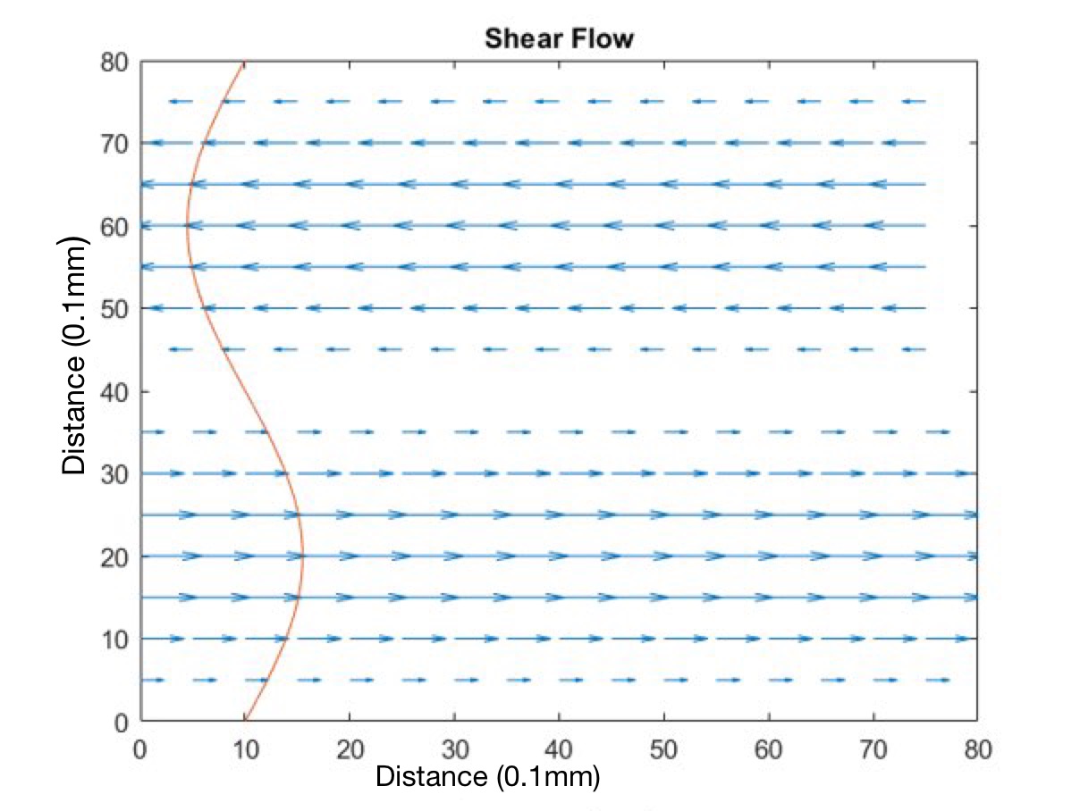
Figure 3. Shear strength multiplied by $dt=0.01s$.

There are two less standard aspects in the simulation of the system (1.1). The first aspect is approximating the shear flow advection, and the second is calculating the aggregation towards the chemoattractant.

For the first issue, we take $u(y)=\sin(2\pi(y-L/2)/L);$ recall that the target is located at $y=L/2,$ so the fluid flow can be thought of as taken relative to the target (Figure 3). For very large amplitudes of $A$ (specifically we took $800$ as threshold in the simulation), we saturate the value of the shear replacing $Au(Y_{t})$ with $800\frac{Au(Y_{t})}{|Au(Y_{t})|}$ if $|Au(Y_{t})|>800.$ We do this in order not to take the time step excessively small. We ran several simulations to check that this cutoff procedure does not affect the expected hit time. From our experiments, it appears that only the structure of $u$ near the target (basically just the shear rate) meaningfully affects the result.

Next, we calculate the chemoattractant distribution $c$, which in turn determines the aggregation. The standard finite difference method is applied. We use the five-point stencil method to approximate the Laplacian and the central difference method to discretize the advection $Au(y)\partial_{x}c$. By inverting the linear system corresponding to the discretized elliptic PDE satisfied by the chemical density, we obtain the numerical value of $c$ on the grid points. The numerical chemical gradient can be obtained through standard finite difference. However, interpolation is needed to determine the chemical gradient on the point away from the grid point. The explicit scheme is as follows. For a fixed position $(x_{0},y_{0})$, we first identify $36(=6\times 6)$ grid points in its neighborhood. Then we apply the cubic spline interpolation to determine the gradient value at the point $(x_{0},y_{0})$. Finally, the Euler-Maruyama method is applied to simulate the SDE (1.1i).

In Figure 4A, we illustrate that as the shear rate increases, the distribution of the chemical, as expected, gets stretched in the horizontal direction. In Figure 4B, we plot the chemical gradient vector.

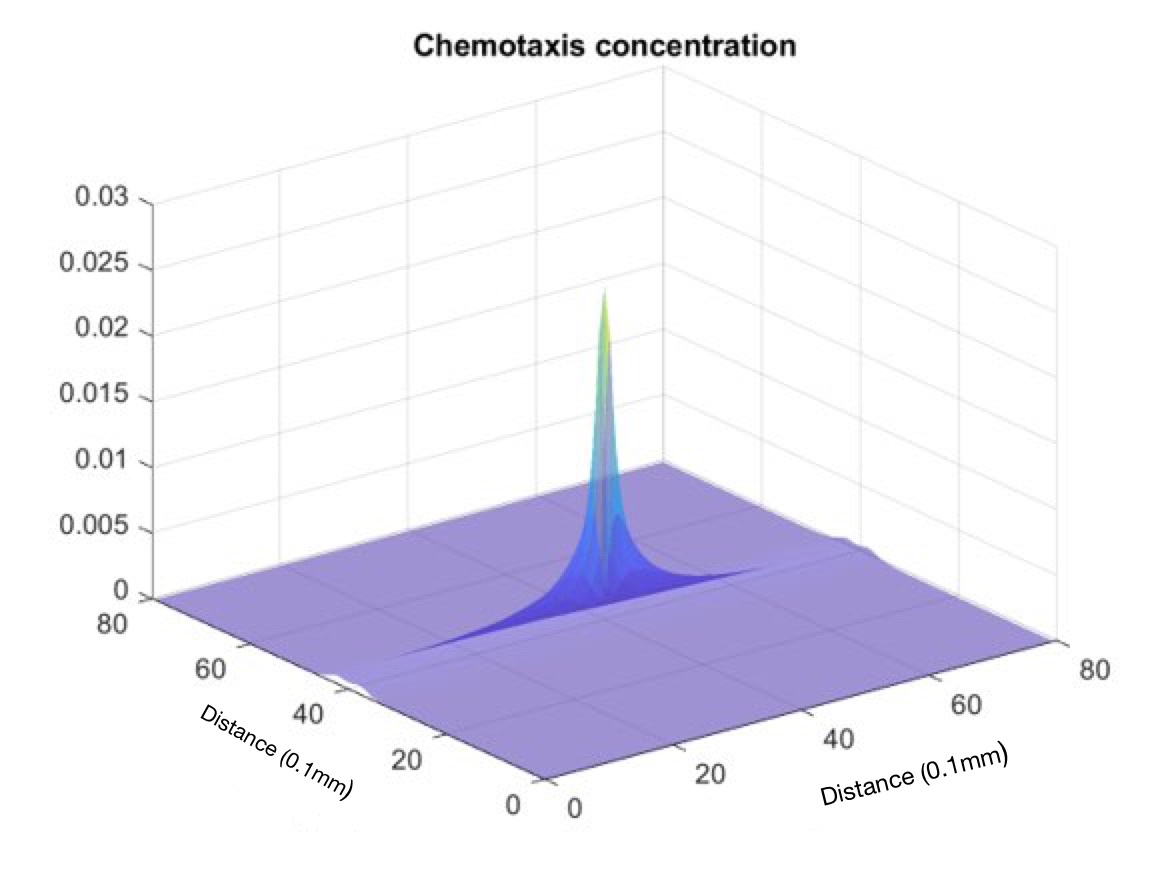
A Chemical concentration $c$

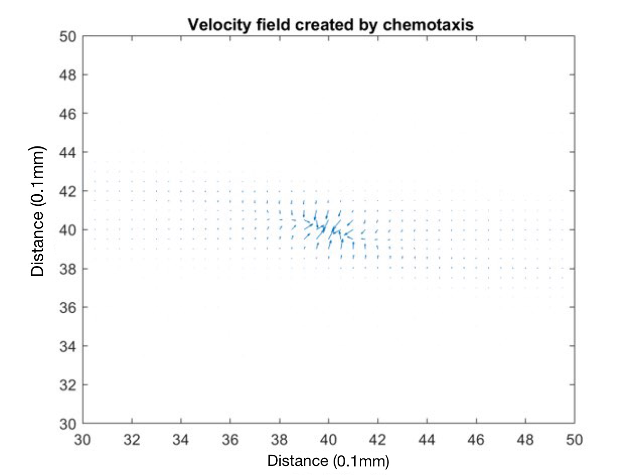
B Chemical gradient $\nabla c$

Figure 4. Chemotaxis concentration and gradient under the effect of shear flow. Boxsize is $80\ (0.1mm)$ and shear amplitude cutoff is set to $200\ (0.1mm)/s$. Based on $2000$ simulations.

3. Numerical Results

3.1. Ranges of parameters

We try to roughly align the ranges of our parameters with the corresponding ranges in the biological experiments of Zimmer and Riffell [31] - at least where these biological parameters are known or can be roughly estimated. The shear rate in our simulation is defined as the ratio $2\pi A/L$. The typical abalone egg diameter is $0.2mm$. The Taylor-Couette tank used in the experiment has distance of about $8$mm between concentric cylinders, and the shear rates tested range between $0$ and $10{\rm s}^{-1}.$ Our simulation covers these ranges of parameters and more. The maximal chemotactic speed $\|\varphi\|_{\infty}$ is limited by the sperm speed ability, which is $v_{0}\sim 0.05$mm/s. One parameter that is not immediate to estimate is the effective diffusion coefficient. There is a large number of results in the literature that rigorously deduce effective diffusion-type equations from the underlying velocity-jump processes describing individual agents - see for example [13, 22] for such derivations in the biological context. However, a limiting asymptotic assumption is necessarily involved in such a transition. We are not aware of the studies on sperm motion that would support a particular model for the change in direction. For this reason we adapt a very simplistic heuristic estimate of the diffusion coefficient outlined below. In the absence of chemical stimuli, sperm appear to move in some direction for a while, then change the direction randomly. Let $t$ be the time that sperm maintains direction. Assuming that sperm maintain speed comparable to maximal, over the larger time $T=nt,$ the displacement $D_{T}$ is given by $D_{T}=\sum_{i=1}^{n}X_{i},$ where $X_{i}$ are independent 2D random variables with amplitude $v_{0}t$ and random direction uniformly distributed over $[0,2\pi).$ We can estimate the expected displacement by

$$\mathbb{E}(D_{T}^{2})=\mathbb{E}\left(\sum_{i=1}^{n}X_{i}\cdot\sum_{j=1}^{n}X_{j}\right)=n\mathbb{E}(X_{i}^{2})=nv_{0}^{2}t^{2}=Tv_{0}^{2}t.$$

Now for a 2D Brownian motion, we have $\mathbb{E}(B_{T}^{2})=4\nu T,$ where $\nu$ is diffusion coefficient. Thus in two dimensions it is reasonable to adopt an estimate $\nu=\frac{1}{4}v_{0}^{2}t.$ The only parameter that we do not have readily available is $t$, but looking at the trajectories of sperm motion provided in [31], taking $t\sim 1$s appears to be reasonable. This leads to the estimate $\nu\approx 0.06(0.1{\rm mm})^{2}/{\rm s}.$ In the numerical simulation, we choose not to have a very small diffusion coefficient and pick $\nu_{\mathrm{num}}=0.25,$ which is equivalent to changing numerical unit time from one second to roughly $4$ second units. Two parameters in the Table 1 that get affected are the shear rate and maximal chemotactic speed, that in the new units range $0-600(4s)^{-1}$ and $0-5(0.1mm)/(4s)$ (respectively $0-150s^{-1}$ and $0-1.25(0.1mm)/s$ in natural units) in our simulation. One parameter that we cannot estimate from the biological experiment is the chemical sensitivity $\chi.$ Although the parameter ranges are coordinated with the experiment [31], we find it likely that they are relevant in a wider range of biological applications. While we use $4s$ time units in parameter table, on our plots we make an adjustment to more natural time units of just seconds. We do keep the $0.1mm$ length unit on the plots since this unit is the intrinsic target size parameter rather than a numerical artifact.

Parameters	Value/Range in Biology	Value/Range in Simulation
Diffusion Coefficient	$\sim 0.06$ $(0.1mm)^{2}/s$	$0.25$ $(0.1mm)^{2}/(4s)$
Egg Radius	$1$ ($0.1mm$)	$1$ ($0.1mm)$
Box Size	$\sim 80$ ($0.1mm$)	$50-200$ ($0.1mm$)
Shear Rate	$0-12$ ($s^{-1}$)	$0-600$ $(4s)^{-1}$
Chemical Sensitivity	not clear	$50-50000(0.1mm)$
Maximal chemotactic speed	$\sim 0.5$ (0.1mm/s)	$0-5\ (0.1mm)/(4s)$

Table 1. Parameters

3.2. Brownian motion subject to shear flow

If there is no chemical attraction, i.e., $\chi=0$, the average first hitting time is monotone decreasing in terms of the shear rate (Figure 5). Moreover, significant decay happens already at the relatively small values of shear rate (note the logarithmic scale of the graph). For large shear rates, the expected hitting time approaches the hitting time of 1D Brownian motion where the $x$ coordinate is eliminated (drawn as a line on the graph). The explicit formula for this 1D hitting time is well known and equal to $\frac{1}{\nu}\left(\frac{L}{2}-\delta\right)^{2}$ (see the argument before (5.6) for a sketch).

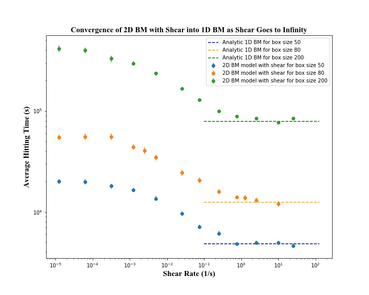
Figure 5. First hitting time with increasing shear rate. Shear amplitude cutoff is set to $200\ (0.1mm)/s$. Chemotaxis is not present.

We refer to [4] for more detailed information on a similar simulation.

3.3. Brownian motion subject to shear flow and chemical attraction: optimal shear

We carry out simulations in tori with three different sizes: $50$, $80$, $200\ (0.1mm)$. In the Figures 6A, 6B and 6C we compare the behavior of the expected hitting time dependence on shear amplitude without chemotaxis and with the maximal chemotaxis speed in the range we analyze. The expected time is computed by averaging over $1000-2000$ simulations, and the vertical bars at each point are two standard deviations of the sample in each direction. In all these simulations, presence of chemotaxis results in more than double reduction of the expected hitting time even when shear is zero. Even very small values of shear rate lead to further meaningful reduction of expected hitting time. The optimal value of the shear rate is in all cases around $0.15-0.3s^{-1}.$ This indicates that the optimal shear value is not affected by the ambient box size. At optimal shear rate, the expected hitting time is reduced more than by another factor of two, and by about a third (less for the largest box) outperforms the one-dimensional large shear rate limit. The value of this limit is indicated on the plots as a solid line. Note that this is a large shear limit without chemotaxis, which is explicitly computable. Our results in the analytic section rigorously establish that the expected search time converges in the large $A$ limit to 1D problem with effective chemotaxis. However, our numerical simulations suggest that the 1D hitting time of this 1D effective chemotaxis problem is quite close to that of the 1D diffusion without chemotaxis - at least within our ranges of parameters. The figures 6A, 6A and 6A give an impression that the optimal shear effect becomes less pronounced with increasing box size. Indeed, the minimal and the large $A$ limit expected time ratios are approximately $3370/4610\sim 73\%,$ $7880/12170\sim 65\%,$ and $70400/78400\sim 90\%$ for the box sizes $50,$ $80,$ and $200.$ One can conjecture that the effect of chemotaxis is relatively short range in the vertical direction, and so for very large box size any possible gain compared to the 1D effective problem is going to be limited.

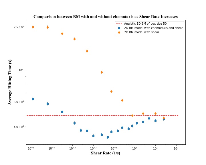
A First hitting time with shear flow and
chemical attraction: Box size 50 (0.1 mm).

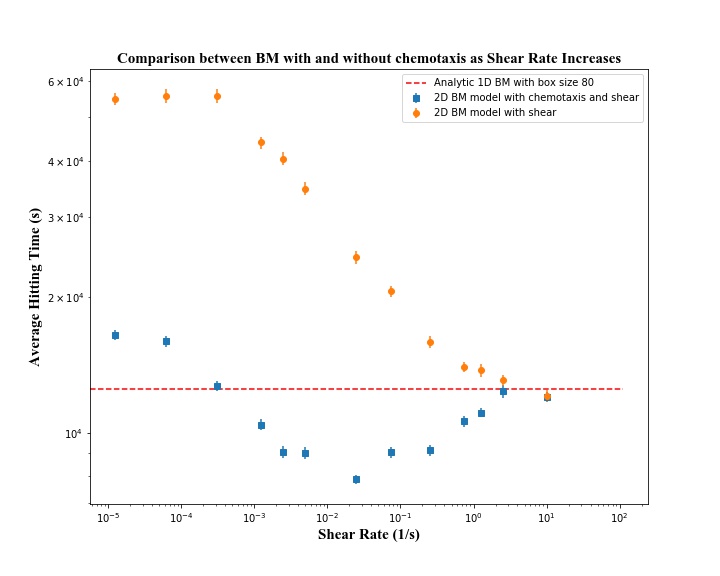
B First hitting time with shear flow and
chemical attraction: Box size 80 (0.1 mm).

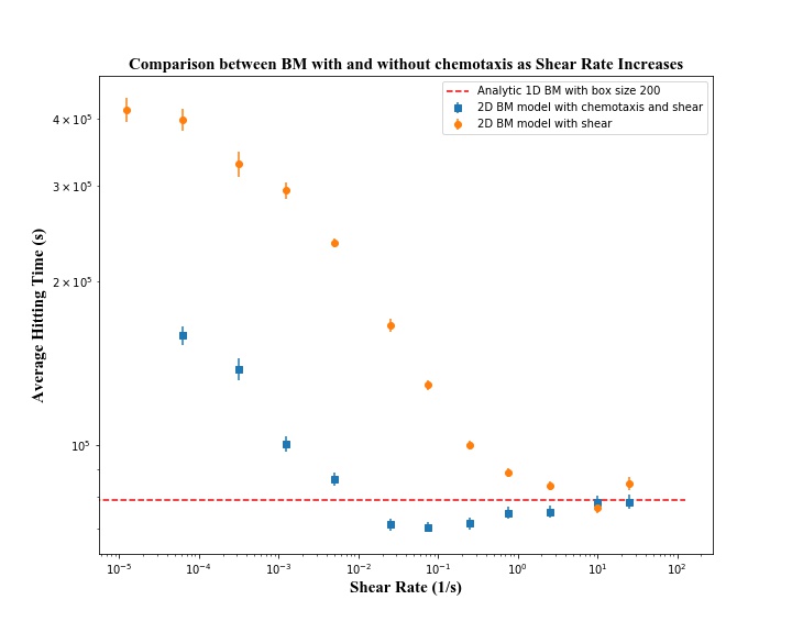
C First hitting time with shear flow and
chemical attraction: Box size 200 (0.1 mm).

Figure 6. First hitting time with shear flow and chemical attraction in different box sizes. Shear amplitude cutoff is set to $200\ (0.1mm)/s$, chemotaxis sensitivity $\chi=500\ (0.1mm)$, chemotaxis cutoff $||\varphi||_{\infty}=1.25\ (0.1mm)/s$. Based on $2000$ simulations.

In Figure 7, we explore the dependence of the expected hitting time on shear rate for different values of maximal chemotactic speed. Here the box size is taken to be $50$ $(0.1)mm$, where the effects we are going to describe are most pronounced (but they are similar for larger boxes). The first interesting phenomena we observe is that beyond certain point, increasing $\|\varphi\|_{\infty}$ does not have much effect on expected hitting time: values $0.125,$ $0.25$ (not pictured) and $1.25$ $(0.1mm/s)$ lead to very close outcomes. Due to piecewise linear structure of $\varphi,$ the maximal chemotactic speed applies only where the gradient of the chemical $c$ is maximal, meaning near the target. Although in our simulations this region is not void, apparently it is not sufficiently expansive even for fairly large sensitivity to meaningfully affect the expected hitting time. Other interesting effects we observe are quite wide range of shear rates where the agent performance exceeds the limiting one-dimensional large shear rate expected search time (the plateau effect), and the drift in the value of optimal shear rate depending on the maximal chemotactic speed.

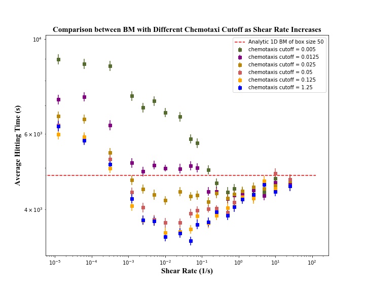
Figure 7. Average first hitting time with varying chemical cut-off $||\varphi||_{\infty}$ and shear rate $A/L$. Box size is $50\ (0.1mm)$, shear amplitude cutoff is set to $200\ (0.1mm)/s$, and chemotaxis sensitivity $\chi=500\ (0.1mm)$.

The Figure 8A illustrates the plateau effect, and shows that for shear rates between $0.015$ and $60$ $s^{-1},$ the agent meaningfully outperforms the limiting one-dimensional large shear rate expected search time for all chemotactic maximal speeds from $0.025$ to $1.25$ $(0.1mm/s)$. For small chemotactic maximal speeds such as $0.025$ $(0.1mm/s)$, the expected hitting time values form an almost constant plateau for this entire range, meaning that even very small values of shear rate combined with very small chemotactic speed are preferable to the dimensional reduction of very high shear rates. We note that sharp improvement in the agent’s search ability even for small values of shear and maximal chemotactic speed are in complete agreement with the results of biological experiments by Riffell and Zimmar. As we mentioned before, the fertilization rate success in their experiments starts falling for large values of shear much more dramatically than we observe in our computations. But this is natural: as discussed in the papers [25], [26], [31], in the fast shear environment, strong shear flows triggers spinning of the searching sperms. As a result, the sperms are less likely to attach to the eggs and succeed in fertilization. Hence the fertilization process often fails in the fast shear regime. However, the spinning effect is not taken into account in our numerical simulation. Nevertheless, we observe the great enhancement of the searching functions for small parameters and the optimal shear rate effect even in the context of our fundamental model, which suggests that these effects are prevalent across many different settings in biology.

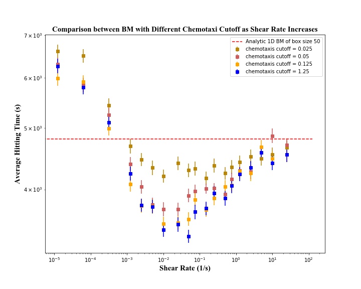
A Plateau effect

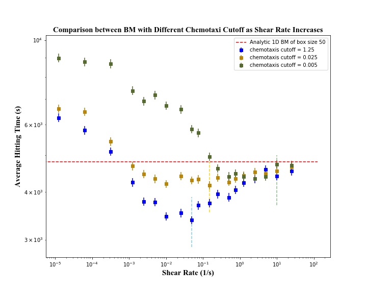
B Changes of optimal shear rate

Figure 8. Plateau effect and changes of optimal shear rate under different chemotaxis cutoff Boxsize is $80\ (0.1mm)$ and shear amplitude cutoff is set to $200\ (0.1mm)/s$.

The Figure 8B illustrates the dependence of the optimal shear value on chemotactic maximal speed. A natural conjecture is whether the combined effect of shear and chemotaxis is strongest at the threshold where the agent is just able to outswim the shear flow in the neighborhood of the target. Indeed, if the shear becomes too strong it may nullify the ability of the agent to benefit from the chemical signal even if it is perceptible. However if this simple mechanism was indeed accurate, we should observe the decline in the optimal shear value when chemotactic maximal speed declines. We could not isolate the parameter regime where such phenomenon would be clearly observable. Apparently, the interaction between shear and chemotaxis is more nuanced and subtle. It appears that for the strong and moderate values of chemotactic maximal speeds, the optimal shear values were comparable, in $\sim 0.06-0.3s^{-1}$ range. For the small values of maximal chemotactic speed, the optimal shear value tended to go up, not down. For example, for the maximal speed $0.005mm/s,$ the optimal shear value is around $1.5s^{-1}.$ The benefit of the shear flow appears to outweigh inability of the agent to go against it for small values of maximal chemotactic speed - up to a point. Very strong shears lead to expected times close to the effective 1D problem for all values of maximal chemotactic speed (at least in the range considered in this paper).

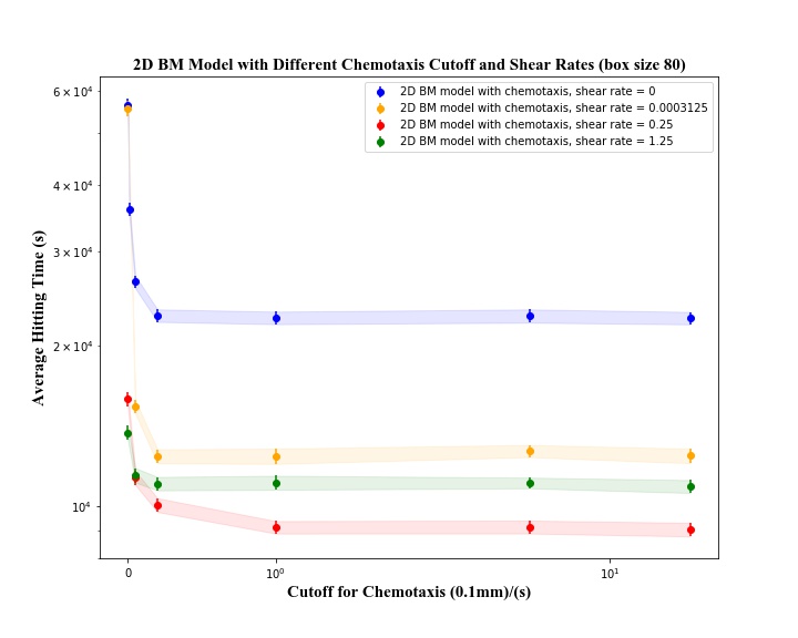
Figure 9. Average first hitting time with varying chemical cut-off $||\varphi||_{\infty}$ and shear rate $A/L$. Boxsize is $80\ (0.1mm)$, shear amplitude cutoff is set to $200\ (0.1mm)/s$, and chemotaxis sensitivity $\chi=500\ (0.1mm)$.

In Figure 9, we provide a different perspective on the same phenomena - here the expected hitting time is plotted as a function of maximal chemotactic speed for different values of shear rate. We see that initially increasing shear rate leads to decrease in the expected hit time, but then it starts going in the opposite direction for all but the smallest values of the maximal chemotactic speed.

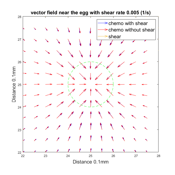
A Shear rate = 0.03 $(s)^{-1}$

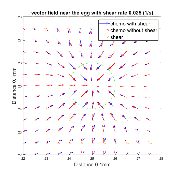
B Shear rate = 0.15 $(s)^{-1}$

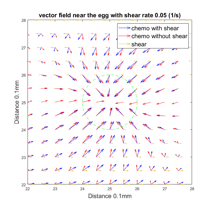
C Shear rate = 0.3 $(s)^{-1}$(Optimal)

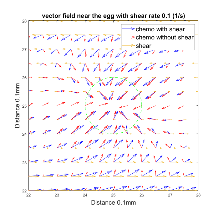
D Shear rate = 0.6 $(s)^{-1}$

Figure 10. Vector fields around the egg with different shear rates in a box of size $50\ (0.1mm)$. Shear amplitude cutoff is set to $200\ (0.1mm)/s$, chemotaxis sensitivity $\chi=500\ (0.1mm)$, chemotaxis cutoff $||\varphi||_{\infty}=1.25\ (0.1mm)/s$.

To further understand the optimal shear rate effect, we performed a numeric experiment without Brownian motion:

(3.1g) $$\left(\begin{array}[]{rr}dX_{t}\\ dY_{t}\end{array}\right)= \left(\begin{array}[]{cc}{A}u(Y_{t})\\ 0\end{array}\right)dt+\left(\begin{array}[]{c}V^{(1)}\\ V^{(2)}\end{array}\right)dt;$$

(3.1h) $$V= (V^{(1)},V^{(2)})=\varphi({\chi}|\nabla c|)\frac{\nabla c}{|\nabla c|},\quad-\Delta c+{A}u(y)\partial_{x}c=n-c.$$

This system involves the interaction of shear and chemotaxis only, and so it is deterministic. Note that in (3.1), there is no guarantee that agent will find the target at all. The result depends on the initial location of the agent. We consider a sample of agents equally spaced along the vertical axis at $x=0$ (recall that the target is located at $(L/2,L/2)$). Instead of computing the search time, we find the percentage of agents that do hit the target within a sufficiently large time frame. In Figure 10, we can see the vector fields near the egg with different shear rates in a box of size $50\ (0.1mm)$. The arrows in yellow represent vector field created by shear flow, the arrow in red represent the vector field created by chemotaxis (note that the effect of shear is still present when we numerically solved for chemical gradient), and the arrows in blue present the sum of shear and chemoattrant vector fields.

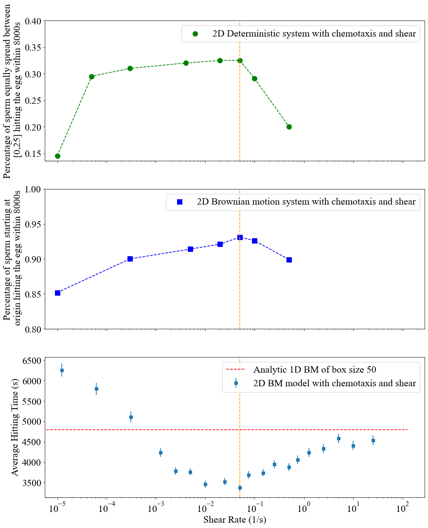
Figure 11. Effect of chemotaxis and shear in egg-searching process in deterministic system vs. stochastic system in a box of size $50\ (0.1mm)$. Shear amplitude cutoff is set to $200\ (0.1mm)/s$, chemotaxis sensitivity $\chi=500(0.1mm)$, chemotaxis cutoff $||\varphi||_{\infty}=1.25\ (0.1mm)/s$. Yellow dotted line denotes optimal configuration with shear rate $0.3\ (s)^{-1}$.

The maximal agent success rate for this setup happens at values of shear similar to the ones leading to smallest expected hitting time in the simulations with diffusion. In Figure 11, we provide a comparison of simulations without and with diffusion for $L=50\ (0.1mm),$ $\chi=500\ (0.1mm)$ and $\|\varphi\|_{\infty}=1.25\ (0.1mm/s).$ In the simulation without diffusion, we place one agent every $0.01\ (0.1mm)$ distance apart, i.e, there are 2501 agent sampling points in the interval $[0,25],$ and let them evolve according to the system (3.1) for time $8000\ s$. Then we record the number of agents that successfully hit the target in this time frame to obtain Figure 11. This simulation in deterministic system gives a natural parallel to the phenomenon we observed in the stochastic system (Figure 6A). Moreover, the optimal shear rates are similar in both cases, and the plateau effect is even more pronounced in the deterministic case. Thus these effects are intrinsic features of interaction between shear flow and chemotaxis.

We also show sample trajectories of the agent right before hitting the target zone (Figure 12). When the shear rate is optimal (0.3 $s^{-1}$), we observe that the searching agent can turn around and approach the target zone. On the other hand, if the shear rate overpowers the chemical attraction, the searching agent can be washed away even though it is right next to the target.

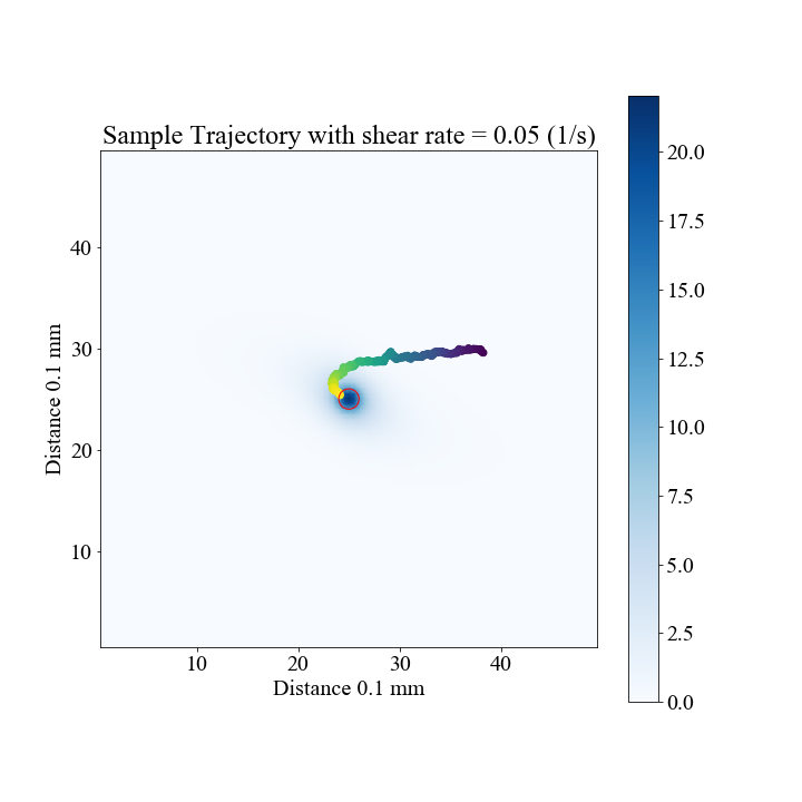
A Shear rate = 0.3 $(s)^{-1}$(Optimal)

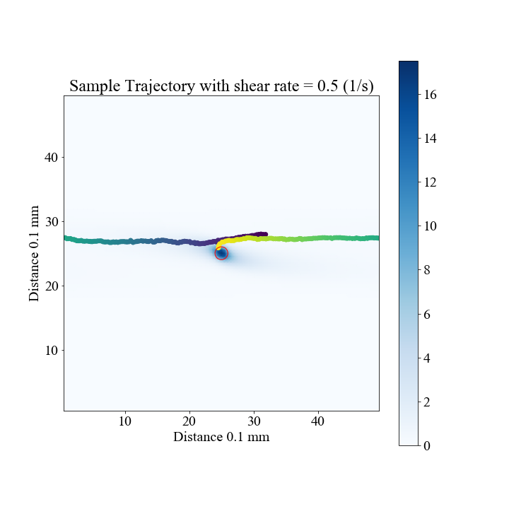
B Shear rate = 3.0 $(s)^{-1}$

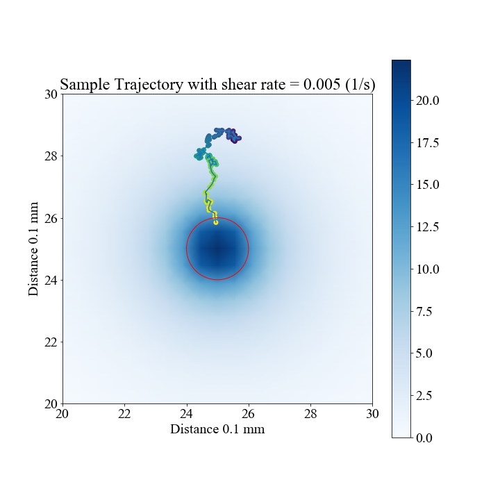
C Shear rate = 0.03 $s^{-1}$

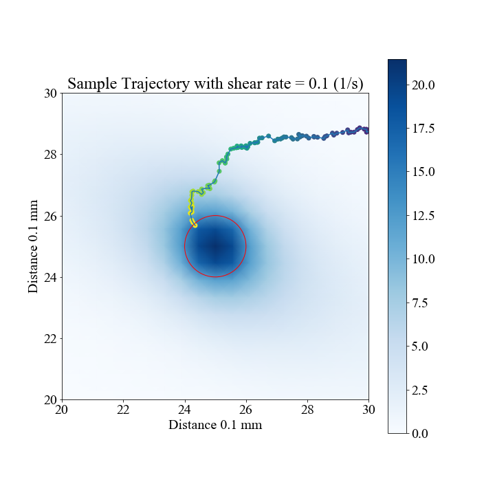
D Shear rate = 0.6 $s^{-1}$

Figure 12. Sample searching trajectories around the egg with different shear rates in a box of size $50\ (0.1mm)$. Chemotaxis sensitivity $\chi=500\ (0.1mm)$, chemotaxis cutoff $||\varphi||_{\infty}=1.25\ (0.1mm)/s$.

To better understand what happens at shear rate values close to optimal, we plot several graphs (Figure 13) that depict the probability distribution of the agent’s hitting points on the surface of the target parameterized by the approach angle $\theta$ (with and without chemotaxis and at different values of shear rate). The approach angle $\theta$ is defined as the angle between the first hitting position of the target zone $E$ and the positive direction of the $x$-axis. To compute the approach angle from the discrete trajectory of the searching agent, we identify the first position of the agent after entering the target zone. Then we interpolate between this entering position and the agent’s previous position in the simulation. The interpolation line will intersect the boundary of the egg zone at a point. The approach angle is calculated using this intersection point.

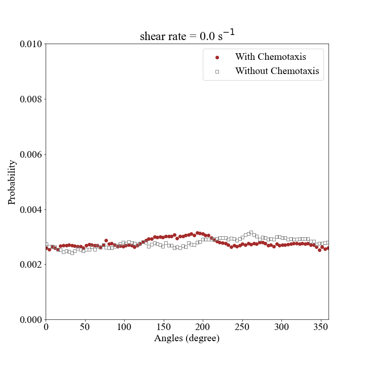
A Shear rate = 0 $s^{-1}$

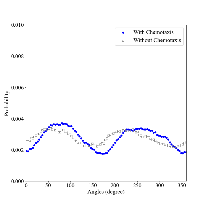
B Shear rate = 0.03 $s^{-1}$

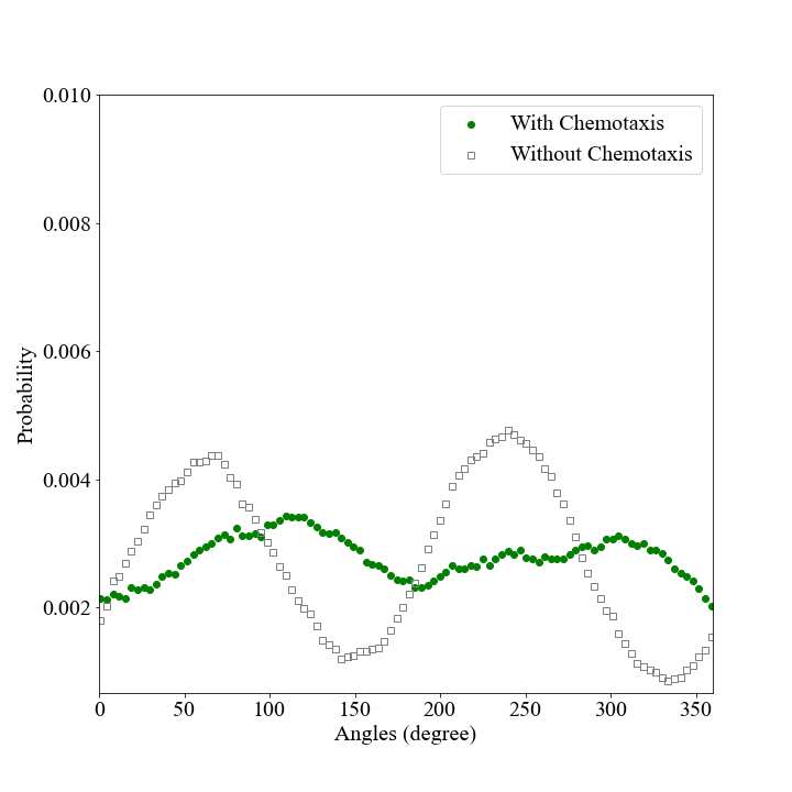
C Shear rate = 0.3 $s^{-1}$

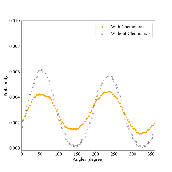
D Shear rate = 3.0 $s^{-1}$

Figure 13. The empirical distribution of the approach angle with and without chemotaxis for varying shear rates

At zero shear rate, the distribution of the approach angles is close to uniform both with and without chemotaxis. For small values of shear rate, the distributions with and without chemotaxis deviate from uniform and start to shift away from each other, although they remain close. For the shear only case hitting the target on the side exposed to the shear becomes more likely than on the protected down flow side, while the angle distribution with chemotaxis begins to shift to the right compared to shear only. At near optimal shear rates, we see an interesting phenomenon in that the peaks of angle distributions with and without chemotaxis are clearly misaligned. Without chemotaxis, the peaks are around $70^{\circ}$ and $250^{\circ},$ which corresponds to the sides exposed to shear flow, and the minima are around $150^{\circ}$ and $330^{\circ}$ corresponding to the protected from shear sides of the target. Both maxima and minima are more pronounced than when chemotaxis is present. With chemotaxis, the maxima shift to about $120^{\circ}$ and $300^{\circ},$ which in fact lie on the down flow parts of the target and are indicative of a large number of trajectories pulled towards the target even after passing it but ending up in the attractive chemical cloud. The minima in the chemotactic case are right around $0^{\circ}$ and $180^{\circ}.$ At high shear rates, the angle distributions with and without chemotaxis become aligned, with extremal points of the approach angle probability distribution with chemotaxis pulled towards those without. This is indicative of a more limited ability for the trajectories to come back from behind against the flow. Some trace of this ability remains though, since although the variation in the probability distribution grows for both cases, in the case with chemotaxis it is less pronounced - which corresponds to more even distribution of hitting points on the surface of the target.

3.4. Chemotactic maximal speed vs sensitivity

We have also explored the role of two key parameters in our chemotaxis model: chemotactic sensitivity and maximal speed cutoff $\|\varphi\|_{\infty}.$ For these simulations, we set shear rate to zero. The main conclusion we can draw from these simulations is that increased sensitivity appears to be more important for reduction of the expected hitting time than maximal chemotactic speed cutoff.

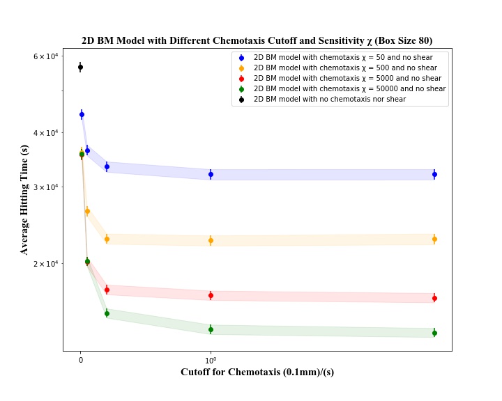
A

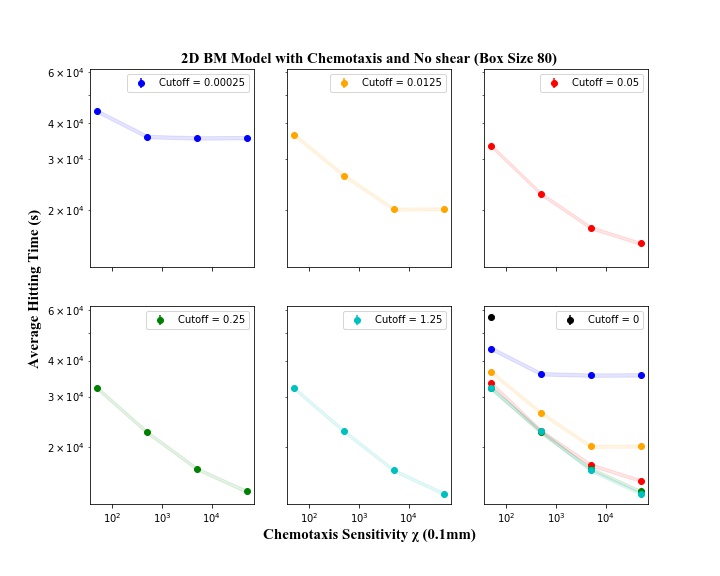
B

Figure 14. Average first hitting time with varying chemical cut-off $\varphi$ and chemical sensitivity $\chi$. Shear flow is not present.

In the Figure 14A, we fix the size of the torus to be $80\ (0.1mm)$ and explore the relationship between the average first hitting time and the maximal chemotactic speed cut-off $||\varphi||_{\infty}$ for different values of chemical sensitivity. We observe that the most of reduction in the expected hitting time happens already before reaching the maximal chemotactic speeds $\sim 0.05-0.1\ (0.1mm/s)$. The additional improvement throughout the tested speed range of up to $0.125mm/s$ is marginal. It should be noted though that even marginal improvement may be important when there is active competition between different agents. On the other hand, Figure 14B shows that increase in chemical sensitivity throughout the whole tested range continues to endow significant advantage to the agents with all but the smallest maximal chemotactic speeds.

4. Mathematical Analysis: Main Results

Throughout this section, we assume the same setting as before: the search takes place on a torus $L{\mathbb{T}}^{2}=[0,L)^{2}.$ The target is a disc of radius $\delta$ located at $(L/2,L/2).$ The agent performs target search in shear flow aided by chemotaxis (of the same form as described in (1.1j)). The only difference with the setting of numerical experiments is that we will not in general assume a certain starting point for the search, but instead will consider expected hitting times with arbitrary initial position. We also choose not to normalize any parameters, and carry $\delta$ and $\nu$ through the estimates.

Let us first consider the case of large $A$ limit when chemotaxis is not present (and the box size $L$ is fixed). One expects that strong shear effectively reduces one dimension. The result we state below is in the spirit of Freidlin-Wentzel theory [10], is likely known and is certainly in the folklore. However we could not find a convenient reference to quote and include the proof for the sake of completeness.

When no chemical aggregation is present, i.e., $\chi=0$, the SDE for the searching agent is simple, i.e.,

(4.7) $$\left(\begin{array}[]{rr}dX_{t}\\ dY_{t}\end{array}\right)= \left(\begin{array}[]{cc}{A}u(Y_{t})\\ 0\end{array}\right)dt+\sqrt{2\nu}\left(\begin{array}[]{cc}dB_{t}^{(1)}\\ dB_{t}^{(2)}\end{array}\right),$$

(4.8) $$(X_{t},Y_{t})= (x_{0},y_{0}).$$

Let $\mathbb{E}^{(x_{0},y_{0})}T_{2D}^{A}$ be the expected time of the process (4.7) on torus ${\mathbb{T}}^{2}=[0,L)^{2}$ starting at $(x_{0},y_{0})$ to hit the target $B((L/2,L/2);\delta)$, namely,

(4.9) $$\mathbb{E}^{(x_{0},y_{0})}T_{2D}^{A}=\mathbb{E}^{(x_{0},y_{0})}\min_{t}\{t|(X_{t},Y_{t})\in B((L/2,L/2);\delta),\quad(X_{t},Y_{t})\text{ solves the SDE }\eqref{Passive_transport_SDE}\}.$$

To capture the large shear behavior of the averaged first hitting time, we define the one-dimensional first hitting time

(4.10) $$T_{1D}=\min_{t}\left\{t\bigg{|}Y_{t}\in\left[\frac{L}{2}-\delta,\frac{L}{2}+\delta\right],\,(X_{t},Y_{t})\text{ solves \eqref{Passive_transport_SDE}. }\right\}.$$

As the shear strength $A$ increases, one expects that the searching agent traverses the horizontal direction fast, and $\mathbb{E}T_{2D}^{A}$ approaches $\mathbb{E}T_{1D}$.

Theorem 1.

Consider the equation (4.7). Suppose the shear profile $u(y)\in C^{2}({\mathbb{T}})$ is such that $u(L/2)=0$. Moreover, assume that

(4.11) $$\min_{y\in[L/2-2\delta,L/2+2\delta]}|u^{\prime}(y)|\geq u_{d}>0.$$

Then the average first hitting time $\mathbb{E}^{(x_{0},y_{0})}T_{2D}^{A}$ (4.9) approaches $\mathbb{E}^{y_{0}}T_{1D}$ (4.10), i.e.,

(4.12) $$\lim_{A\rightarrow\infty}\mathbb{E}^{(x_{0},y_{0})}T_{2D}^{A}=\mathbb{E}^{y_{0}}T_{1D}.$$

Remark 1.

In our simulation, $u(y)=\sin(2\pi(y-L/2)/L),$ and $u_{d}\sim L^{-1}$.

Remark 2.

It is not hard to show that $\lim_{A\rightarrow\infty}T_{2D}^{A}(\omega)=T_{1D}(\omega)$ almost surely. Indeed, by Blumenthal’s 0-1 law, if we let $\tau=\inf\{t\geq 0:B_{t}>0\},$ then $\mathbb{P}_{0}(\tau=0)=1$ see e.g. [8]. So once we reach one of the levels $y-L/2=\pm\delta$ at $T_{1D}(\omega),$ by almost sure continuity of Brownian motion, with probability one there is an interval of times arbitrarily close to the time $T_{1D}(\omega)$ during which we will dip into the target zone $|y-L/2|<\delta.$ Thus as $A\rightarrow\infty,$ $T_{2D}^{A}(\omega)$ will converge to $T_{1D}(\omega).$

If there exists chemical attraction $(\chi\neq 0)$, the analysis is more involved. As the magnitude of the shear flow $Au(y)$ increases, the chemical gradient $\nabla c$ homogenizes in the horizontal direction. Hence the attraction vector field $V$ is also homogenized in the $x$-direction. To explicitly capture the homogenization effect, we consider the elliptic equation on $(x,y)\in L{\mathbb{T}}\times L{\mathbb{T}}$:

(4.13) $$-\Delta c+Au(y)\partial_{x}c=n-c.$$

As before, we assume that the target density $n$ is stationary and its support is localized near the center of the torus, i.e.,

(4.14) $$\{y|(x,y)\in\mathrm{support}\{n\}\}=B_{\delta}(L/2,L/2)$$

Moreover, the shear flow $u(y)$ will be assumed to be strictly monotone in the neighborhood of the support of $n$, i.e., satisfy (4.11).

Next we introduce the horizontal-homogenization. Functions $f$ on $L{\mathbb{T}}\times L{\mathbb{T}}$ can be decomposed into $x$-average $\langle f\rangle$ and the remainder $f_{\sim}$:

(4.15) $$\langle f\rangle(y)=\frac{1}{L}\int_{0}^{L}f(x,y)dx,\quad f_{\sim}(x,y)=f(x,y)-\langle f\rangle(y).$$

The remainder of the chemical $c_{\sim}$ will be homogenized in the $x$-direction in the sense that $c_{\sim},\,\nabla c_{\sim}$ decay to zero as $A$ approaches infinity. The results are summarized in the next theorem.

Theorem 2.

Consider the solutions $c$ to the equation (4.13). The shear flow profile $u\in C^{2}({\mathbb{T}})$ has only finitely many critical points and is non-degenerate in the sense that if $u^{\prime}(y_{0})=0$ at a point $y_{0}$, then $u^{\prime\prime}(y_{0})\neq 0$. Further assume that the shear profile is strictly monotone near the egg zone (4.11) and the egg density is localized (4.14). Then the chemical density $c_{\sim}$ and its derivatives up to the second order are approaching zero as $A$ approaches infinity, i.e.,

(4.16) $$||\partial_{x}^{i}c_{\sim}||_{\infty}\leq\frac{C|\log A|||\partial_{x}^{i}n_{\sim}||_{\infty}}{A^{2/3}},\quad||\partial_{x}^{j}\partial_{y}c_{\sim}||_{\infty}\leq\frac{C|\log A|^{2}||\partial_{x}^{j}\nabla n_{\sim}||_{\infty}}{A^{1/6}},\quad i\in\{0,1,2\},\,j\in\{0,1\}.$$

Here the constant $C$ depends on the parameters $\nu,\,L$.

Now we consider the convergence of the average first hitting time in the full generality ($\chi\neq 0$). We use the notation $T^{A;\chi}_{2D}$ to denote the first hitting time of the SDE (1.1), namely,

(4.17) $$T_{2D}^{A;\chi}=\min_{t}\{t|(X_{t},Y_{t})\in B((L/2,L/2);\delta),\quad(X_{t},Y_{t})\text{ solves the SDE }\eqref{SDE_full}\}.$$

Next we define the effective $1D$ system

(4.18) $$dY_{t}=V_{\mathrm{eff}}^{(2)}dt+\sqrt{\nu}dB_{t},\quad V_{\mathrm{eff}}^{(2)}=\varphi(\chi|\partial_{y}\langle c\rangle|)\frac{\partial_{y}\langle c\rangle}{|\partial_{y}\langle c\rangle|},\quad Y_{0}=y_{0}.$$

Observe that $\langle c\rangle(y)$ solves a simple PDE

$$\partial^{2}_{y}\langle c\rangle=\langle n\rangle-\langle c\rangle.$$

We define the $1D$-first hitting time as follows

(4.19) $$T_{1D}^{\chi}=\min_{t}\left\{t\bigg{|}Y_{t}\in\left[\frac{L}{2}-\delta,\frac{L}{2}+\delta\right],\,Y_{t}\text{ solves \eqref{1D_effective_SDE}. }\right\}.$$

The value of $\mathbb{E}^{y_{0}}T_{1D}^{\chi}$ can be calculated using Dynkin’s formula and integration factor method; we will outline this computation in Section 7.

Theorem 3.

Consider the dynamics (1.1). Assume that the density $n\in C^{2}({\mathbb{T}}^{2})$, and the cutoff function ${\varphi(\cdot)}\in C^{2}(\mathbb{R}_{+})$ vanishes at the origin, i.e., $\varphi(0)=0$. The shear profile $u\in C^{2}({\mathbb{T}})$ satisfies all assumptions in Theorem 1 and 2. Then the expected first hitting time $\mathbb{E}^{(x_{0},y_{0})}T_{2D}^{A;\chi}$ (4.17) approaches the expected $1D$-first hitting time $\mathbb{E}^{y_{0}}T_{1D}^{\chi}$ (4.19) as the magnitude $A$ tends to infinity, i.e.,

(4.20) $$\lim_{A\rightarrow\infty}\mathbb{E}^{(x_{0},y_{0})}T_{2D}^{A;\chi}=\mathbb{E}^{y_{0}}T_{1D}^{\chi},\quad\forall(x_{0},y_{0})\in(L{\mathbb{T}})^{2}.$$

Remark 3.

In fact, explicit convergence rate will be derived in Section 7.

5. Proof of Theorem 1

If $\chi=0$, it is well known how to calculate the expected first hitting time $\mathbb{E}^{y_{0}}T_{1D}$ (4.10). Since only the $y$-component of the agent’s position determines whether the agent hit the target region $\left[\frac{L}{2}-\delta,\frac{L}{2}+\delta\right]$, it is enough to consider the SDE $dY_{t}=\sqrt{2\nu}B_{t}^{(2)}$. The agent starts at $y_{0},$ and performs the Brownian motion $\sqrt{2\nu}dB_{t}$ on $[0,L)$ with periodic boundary conditions until it hits the interval $[\frac{L}{2}-\delta,\frac{L}{2}+\delta].$ We can recast this problem equivalently as the exit time from $[-L/2+\delta,L/2-\delta]$ for a Brownian particle starting at $y_{0}$ (without loss of generality we assume that $y<L/2$). The expected first exit time is well known and can be computed explicitly; we provide a brief sketch of the argument. First recall the Dynkin formula ([21]): for $f\in C_{0}^{2}$, suppose $\tau$ is a stopping time, $\mathbb{E}^{y_{0}}[\tau]<\infty$, then

(5.1) $$\mathbb{E}^{y_{0}}[f(Y_{\tau})]=f(y_{0})+\mathbb{E}^{y_{0}}\left[\int_{0}^{\tau}Hf(Y_{s})ds\right],$$

where in our case

(5.2) $$dY_{t}=\sqrt{2\nu}dB_{t},\quad Hf=\nu\partial_{yy}f,\quad Y_{0}=y_{0}.$$

To apply the formula, we consider the solution $f$ to the partial differential equation:

(5.3) $${\nu}\partial_{yy}f=-1,\quad f\left(\pm\frac{L}{2}\mp\delta\right)=0.$$

Combining the equation and the formula (5.1), we have obtained the relation

(5.4) $$0={\color[rgb]{0,0,0}\mathbb{E}^{y_{0}}[f(Y_{\tau})]}=f(y_{0})+\mathbb{E}^{y_{0}}\left[\int_{0}^{\tau}Hf(Y_{s})ds\right]=f(y_{0})-\mathbb{E}^{y_{0}}\left[\tau\right],$$

which in turn yields that

(5.5) $$f(y_{0})=\mathbb{E}^{y_{0}}[\tau].$$

Directly solving the equation yields that

(5.6) $$\mathbb{E}^{y_{0}}T_{1D}=\mathbb{E}^{y_{0}}[\tau]=f(y_{0})=-\frac{1}{2\nu}y^{2}_{0}+\frac{1}{2\nu}\left(\frac{L}{2}-\delta\right)^{2}.$$

Now we prove Theorem 1.

Proof of Theorem 1.

For simplicity, we will provide below an argument for the agent starting at $(0,0).$ It can be generalized to $(x_{0},y_{0})$ with $y_{0}\notin[\frac{L}{2}-\delta,\frac{L}{2}+\delta]$ in a straightforward manner. For $y_{0}\in[\frac{L}{2}-\delta,\frac{L}{2}+\delta]$, the argument is similar, but extra modifications are required. We will comment on the adjustments at the end of the proof.

First note that the expected 2D hitting time is larger than the 1D hitting time. This can be seen through considering the $y$-component. If $Y_{t}$ does not reach the region $[\frac{L}{2}-\delta,\frac{L}{2}+\delta]$, then the agent does not find the target. Hence the 2D hitting time is bounded below by the 1D hitting time.

To derive an upper bound, let us focus on the searching strips

$$S^{+}=\left\{(x,y)\bigg{|}y\in\left[\frac{L}{2}+\delta-2A^{-1/3},\frac{L}{2}+\delta\right]\right\}\,\,\,{\rm and}\,\,\,S^{-}=\left\{(x,y)\bigg{|}y\in\left[\frac{L}{2}-\delta,\frac{L}{2}-\delta+2A^{-1/3}\right]\right\}.$$

These two strips are adjacent to the boundary of the target zone $y=\frac{L}{2}\pm\delta$. Due to our assumptions $u(L/2)=0$ and (4.11), and assuming that $A$ is sufficiently large, for the values of $y$ within the searching strips $S^{\pm}$ the magnitude of the velocity $u$ has a lower bound. We denote it by

(5.7) $$u_{m}:=\min_{y\in S^{\pm}}|u(y)|\geq\frac{\delta u_{d}}{2}>0.$$

Denote the center levels of $S^{\pm}$ as $y^{\pm}=\frac{L}{2}\pm\delta\mp A^{-1/3}$ respectively.

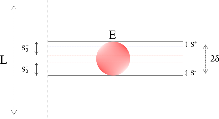
Figure 15. Setup

The expectation of the first hitting time $\tau_{0}$ of the second component getting from $(0,0)$ to one of the center levels $y^{\pm}$ can be explicitly computed similarly to (5.6). Applying the formula analogous to (5.6) but replacing $L/2-\delta$ with $L/2-\delta+A^{-1/3}$, we obtain that

(5.8) $$\mathbb{E}[\tau_{0}]=\frac{1}{2\nu}\left(\frac{L}{2}-\delta+A^{-1/3}\right)^{2}.$$

The two hitting times $\eqref{form}_{y_{0}=0}$, (5.8) differ by a small term of order ${O}(A^{-1/3})$.

Once the agent hits one of the center levels of either $S^{+}$ or $S^{-}$, we will focus on that specific strip. Without loss of generality, we assume that the agent first reaches $y^{+}$. If $A$ is very large, there is a high chance that the agent will hit the target before it exits the strip $S^{+}.$ Indeed, if the agent remains for time $\tau^{in}\geq\frac{2L}{Au_{m}}$ inside $S^{+},$ it has enough time to traverse the entire torus and hit the target. On the other hand, by the reflection principle (see, e.g., equation (3.8) in [7]), we have that

$$\mathbb{P}\left(\tau^{in}\leq\frac{2L}{Au_{m}}\right)=2\mathbb{P}\left(\sqrt{\nu}B_{\frac{2L}{Au_{m}}}\geq A^{-1/3}\right).$$

Since $\mathbb{E}[(B_{t})^{2}]=t,$ the following estimate holds:

$$\mathbb{P}\left(\tau^{in}\leq\frac{2L}{Au_{m}}\right)\leq 2\mathbb{P}\left(\sqrt{\nu}B_{\frac{2L}{Au_{m}}}\geq A^{-1/3}\right)\leq 2\frac{\mathbb{E}\left[\left(B_{\frac{2L}{Au_{m}}}\right)^{2}\right]}{\nu^{-1}A^{-2/3}}\leq\frac{4\nu L}{A^{1/3}u_{m}}.$$

Another possibility is that the $\tau^{in}\geq\frac{2L}{Au_{m}}$, but the agent does not traverse through all the searching strip. The probability of this event is again small. Denoting $X_{e}$ as the entering position and denoting $d_{\mathbb{R}}$ as the distance on the universal cover $\mathbb{R}$ of the torus ${\mathbb{T}}$, we estimate the probability as follows,

$$\mathbb{P}\left(\tau^{in}\geq\frac{2L}{Au_{m}},\,d_{\mathbb{R}}(X_{\frac{2L}{Au_{m}}},X_{e})\leq L\right)\leq\mathbb{P}\left(\sqrt{\nu}B_{\frac{2L}{Au_{m}}}\geq L\right)\leq\frac{2\nu}{Au_{m}L}.$$

We define the event

(5.9) $$F_{i}:=\left\{\tau^{in}\leq\frac{2L}{Au_{m}}\right\}\cup\left\{\tau^{in}\geq\frac{2L}{Au_{m}},d_{\mathbb{R}}(X_{\frac{2L}{Au_{m}}},X_{e})\leq L\right\}.$$

We observe that $F_{i}^{c}$ guarantees a success in the $i$-th trip to $S^{\pm}$.

(5.10) $$\mathbb{P}(F_{i})\leq\mathbb{P}\left(\left\{\tau^{in}\leq\frac{2L}{Au_{m}}\right\}\right)+\mathbb{P}\left(\left\{\tau^{in}\geq\frac{2L}{Au_{m}},d_{\mathbb{R}}(X_{\frac{2L}{Au_{m}}},X_{e})\leq L\right\}\right)\leq\frac{4\nu L}{A^{1/3}u_{m}}+\frac{2\nu}{Au_{m}L}.$$

Now in the event $F_{i}$ we wait for time $\tau^{out}$ till the agent gets back either to the level $y^{+}$ or $y^{-}$. For simplicity we can ignore the option of reaching $y^{-}$ and focus just on $y^{+}.$ Since at the stopping time $\tau^{in},$ the agent is at the boundary of $S^{+},$ analogously with the previous 1D argument, we can compute the expectation of time $\tau^{out}$ by solving the boundary value problem

$$\nu f^{\prime\prime}(z)=-1,\,\,\,f(z=0)=f(z=L)=0,$$

where $\mathbb{E}[\tau^{out}]=f(A^{-1/3}).$ Solving for $f$ yields

$$f(z)=\frac{1}{2\nu}(-z^{2}+Lz),$$

and thus $\mathbb{E}[\tau^{out}]=\frac{1}{2\nu}(LA^{-1/3}-A^{-2/3}).$ Now we can iterate, and by Markov property we obtain

$$\mathbb{E}^{(x_{0},y_{0})}[T_{2D}^{A}]\leq \mathbb{E}[\tau_{0}]+\mathbb{P}\left(F_{1}^{c}\right)\frac{2L}{Au_{m}}+\mathbb{P}\left(F_{1}\right)\left(\mathbb{E}[\tau^{out}]+\mathbb{P}\left(F_{2}^{c}\right)\frac{2L}{Au_{m}}\right)$$

$$+\mathbb{P}\left(F_{1}\right)\mathbb{P}\left(F_{2}\right)\left(\mathbb{E}[\tau^{out}]+\mathbb{P}\left(F_{3}^{c}\right)\frac{2L}{Au_{m}}\right)+...$$

$$= \mathbb{E}[\tau_{0}]+\mathbb{P}\left(F_{1}^{c}\right)\frac{2L}{Au_{m}}+\sum_{i=1}^{\infty}\left(\prod_{j=1}^{i}\mathbb{P}\left(F_{j}\right)\right)\left(\mathbb{E}[\tau^{out}]+\mathbb{P}\left(F_{i+1}^{c}\right)\frac{2L}{Au_{m}}\right).$$

Using our estimates on $\mathbb{E}[\tau^{out}]$, and the fact that $\mathbb{P}(F_{i})<1$ for sufficiently large $A$ (5.10), we find that

$$\mathbb{E}^{(x_{0},y_{0})}[T_{2D}^{A}]\leq \mathbb{E}[\tau_{0}]+C\left(\frac{L}{\nu A^{1/3}}+\frac{2L}{Au_{m}}\right)$$

$$\leq \mathbb{E}[\tau_{0}]+O(A^{-1/3})=\mathbb{E}^{y_{0}}[T_{1D}]+O(A^{-1/3}).$$

Thus the upper bound approaches $\mathbb{E}^{y_{0}}[T_{1D}]$ as $A\rightarrow\infty$.

Finally, we comment on the case where the starting position is in the egg zone level, i.e., $y_{0}\in[L/2-\delta,L/2+\delta]$. In this case, the $1$-dimensional first hitting time is zero. Hence the goal is to show that the average $2$-dimensional first hitting time converges to zero as $A\rightarrow\infty$. We distinguish between two possible cases: case a) $y_{0}\in[L/2-\delta,L/2+\delta]\backslash[L/2-A^{-1/5},L/2+A^{-1/5}]$; case b) $y_{0}\in[L/2-A^{-1/5},L/2+A^{-1/5}]$.

In the first case, without loss of generality, we focus on the upper component $y_{0}\in(L/2+A^{-1/5},L/2+\delta]$. We redefine the searching strip to be $S^{+}:=[y_{0}-2A^{-1/3},y_{0}]$, and note that the center level of $S^{+}$ is $y^{+}:=y_{0}-A^{-1/3}$. Applying the same argument as before, we have that the average first hitting time from $y_{0}$ to $y^{+}$ is bounded above by $\mathbb{E}\tau_{0}\leq CA^{-1/3}$. Inside the searching strip $S^{+}$, the assumptions $u(L/2)=0$, and (4.11) yields that the absolute value of fluid velocity has positive lower bound if $A$ is large enough, i.e.,

$$Au_{m}:= A\min_{y\in S^{+}}|u(y)|\geq Au_{d}(A^{-1/5}-2A^{-1/3})\geq A^{4/5}u_{d}/2.$$

Similarly to the previous argument, we consider the events $F_{i}:=\{\tau^{in}\leq\frac{4L}{A^{4/5}u_{d}}\}\cup\{\tau^{in}\geq\frac{4L}{A^{4/5}u_{d}},\,d_{\mathbb{R}}(X_{\frac{4L}{A^{4/5}u_{d}}},X_{e})\leq L\}$, which are adjustments to definition (5.9). Then the probability of $F_{i}$ can be estimated as follows. First of all,

$$\mathbb{P}\left(\tau^{in}\leq\frac{4L}{A^{4/5}u_{d}}\right)\leq 2\mathbb{P}\left(\sqrt{\nu}B_{\frac{4L}{A^{4/5}u_{d}}}\geq A^{-1/3}\right)\leq 2\frac{\mathbb{E}\left[\left(B_{\frac{4L}{A^{4/5}u_{d}}}\right)^{2}\right]}{\nu^{-1}A^{-2/3}}\leq\frac{8\nu L}{A^{2/15}u_{d}}.$$

Then

$$\mathbb{P}\left(\tau^{in}>\frac{4L}{A^{4/5}u_{d}},\,d_{\mathbb{R}}(X_{\frac{4L}{A^{4/5}u_{d}}},X_{e})\leq L\right)\leq\mathbb{P}\left(\sqrt{\nu}B_{\frac{4L}{A^{4/5}u_{d}}}\geq L\right)\leq\frac{4\nu}{A^{4/5}u_{d}L}.$$

Hence,

$$\mathbb{P}(F_{i})\leq\frac{8\nu L}{A^{2/15}u_{d}}+\frac{4\nu}{A^{4/5}u_{d}L}.$$

Thus $\lim_{A\rightarrow\infty}\mathbb{P}(F_{i})=0$. Now the same iterative argument as above yields the result

$$0\leq\mathbb{E}^{(x_{0},y_{0})}[T_{2D}^{A}]\leq \mathbb{E}[\tau_{0}]+\mathbb{P}\left(F_{1}^{c}\right)\frac{2L}{A^{4/5}u_{d}/2}+\sum_{i=1}^{\infty}\left(\prod_{j=1}^{i}\mathbb{P}\left(F_{j}\right)\right)\left(\mathbb{E}[\tau^{out}]+\mathbb{P}\left(F_{i+1}^{c}\right)\frac{2L}{A^{4/5}u_{d}/2}\right)$$

$$\leq C(\nu,L,u_{d})A^{-2/15}.$$

Therefore, $\lim_{A\rightarrow\infty}\mathbb{E}^{(x_{0},y_{0})}[T_{2D}^{A}]=0$.

If $y_{0}\in[L/2-A^{-1/5},L/2+A^{-1/5}]$, then we define the searching strip to be $S:=[L/2+A^{-1/5}-2A^{-1/3},L/2+A^{-1/5}]$. The average first hitting time from the starting position to the center level $y^{+}:=L/2+A^{-1/5}-A^{-1/3}$ is bounded by $\mathbb{E}[\tau_{0}]\leq CA^{-1/5}$. The speed of the shear inside the searching strip is bounded from below by $Cu_{d}A^{4/5}$. Now the same argument as above completes the proof.

∎

6. Proof of Theorem 2

We first present the enhanced dissipation estimates from the works [2], [30] and [5] adapted to our large torus setting ($|{\mathbb{T}}|=L\gg 1$).

Theorem 4.

Consider solutions $\eta_{\sim}(t,x,y)$ to the passive scalar equations

(6.1) $$\partial_{t}\eta_{\sim}+Au\left(\frac{y}{L}\right)\partial_{x}\eta_{\sim}=\nu\Delta\eta_{\sim},\quad\eta_{\sim}(t=0,x,y)=\eta_{0;\sim}(x,y),\quad\,(x,y)\in{\mathbb{T}}^{2}$$

subject to initial data $\eta_{0;\sim}\in L^{\infty}({\mathbb{T}}^{2})$ and zero average constraint $\int_{{\mathbb{T}}}\eta_{0;\sim}(x,y)dx=0,\,\forall y\in{\mathbb{T}}$.

Case a) Assume that the shear flow profile $u$ is a Lipschitz function with finitely many critical points. Furthermore, if the derivative of the profile exists at a point $y\in{\mathbb{T}}$, then it is strictly bounded away from zero, i.e., $|u^{\prime}(y)|>u_{d}>0$. If the parameter $A$ is large enough in the sense that $\frac{\nu}{AL}\leq c_{0}$ for a small constant $c_{0}=c_{0}(u)>0$, then there exist constants $C,\,\kappa>0$ depending only on the shear profile $u$ such that the following enhanced dissipation estimate holds:

(6.2) $$||\eta_{\sim}(t)||_{\infty}\leq C||\eta_{0;\sim}||_{\infty}e^{-\kappa\nu^{1/3}A^{2/3}L^{-4/3}|\log\frac{\nu}{AL}|^{-1}t},\quad\forall t\in[0,\infty).$$

Case b) The shear flow profile $u\in C^{2}({\mathbb{T}})$ is non-degenerate in the sense that if $u^{\prime}(y_{0})=0$, then $u^{\prime\prime}(y_{0})\neq 0$. Moreover, there are only finitely many critical points. If the parameter $A$ is large enough in the sense that $\frac{\nu}{AL}\leq c_{0}$ for a small constant $c_{0}=c_{0}(u)>0$, then there exist constants $C,\,\kappa>0$ depending only on the shear profile $u$ such that the following enhanced dissipation estimate holds :

(6.3) $$||\eta_{\sim}(t)||_{\infty}\leq C||\eta_{0;\sim}||_{\infty}e^{-\kappa\nu^{1/2}A^{1/2}L^{-3/2}|\log\frac{\nu}{AL}|^{-1}t},\quad\forall t\in[0,\infty).$$

Remark 4.

We will need the estimate (6.2) to derive a sufficiently strong bound on the chemical gradient $||\partial_{y}c_{\sim}||_{\infty}$. We are not able to show that the chemical gradient converges to zero as $A\rightarrow\infty$ using only estimate (6.3).

Proof.

We divide the proof into several steps.

Step # 1: Rescaling argument. If we rescale the variables in (6.1) by setting $X:=\frac{x}{L}$, $Y:=\frac{y}{L}$ and $\tau=\frac{A}{L}t$, we end up with the following:

(6.4) $$\partial_{\tau}\widehat{\eta}_{\sim}+u(Y)\partial_{X}\widehat{\eta}_{\sim}=\widehat{\nu}\Delta_{X,Y}\widehat{\eta}_{\sim},\quad\int_{0}^{1}\widehat{\eta}_{\sim}(x,y)dx=0,\quad(X,Y)\in{\mathbb{T}}^{2}.$$

Here $\widehat{\eta}(\tau,X,Y):=\eta(t,x,y)$, and $\widehat{\nu}:=\frac{\nu}{AL}$. Hence if we obtain the following estimates:

case a)

(6.5) $$||\widehat{\eta}_{\sim}(\tau)||_{L_{X,Y}^{\infty}}\leq C||\widehat{\eta}_{0;\sim}||_{L_{X,Y}^{\infty}}e^{-\kappa_{0}\widehat{\nu}^{1/3}|\log\widehat{\nu}|^{-1}\tau},\quad\forall\tau\in[0,\infty),$$

case b)

(6.6) $$||\widehat{\eta}_{\sim}(\tau)||_{L_{X,Y}^{\infty}}\leq C||\widehat{\eta}_{0;\sim}||_{L_{X,Y}^{\infty}}e^{-\kappa_{0}\widehat{\nu}^{1/2}|\log\widehat{\nu}|^{-1}\tau},\quad\forall\tau\in[0,\infty)$$

for some universal $\kappa_{0},$ then by rescaling back to the original variables, we obtain (6.2) and (6.3).

Step # 2: $L^{2}$-estimates. Consider the passive scalar equation (6.4). We will show that if the viscosity $\widehat{\nu}$ is small enough, i.e., $\widehat{\nu}\leq c_{0}(u)$ for some constant $c_{0}>0$ depending only on $u$, then the enhanced dissipation estimate holds: in case a),

(6.7) $$||\widehat{\eta}_{\sim}(\tau)||_{L^{2}}\leq C||\widehat{\eta}_{0;\sim}||_{L^{2}}e^{-\kappa_{0}\widehat{\nu}^{1/3}\tau},\quad\forall\tau\in[0,\infty);$$

in case b),

(6.8) $$||\widehat{\eta}_{\sim}(\tau)||_{L^{2}}\leq C||\widehat{\eta}_{0;\sim}||_{L^{2}}e^{-\kappa_{0}\widehat{\nu}^{1/2}\tau},\quad\forall\tau\in[0,\infty).$$

Here the constants $C,\,\kappa_{0}$ depend only on the shear profile $u$. The estimate (6.8) appears in Theorem 1.1 of [1]. We also refer the interested readers to [2] and [30].

To prove the (6.7), we first consider the mixed $x$-Fourier transform of the passive scalar equation

$$\partial_{t}\widehat{\eta}_{k}= \widehat{\nu}\partial_{YY}\widehat{\eta}_{k}-\widehat{\nu}|k|^{2}\widehat{\eta}_{k}-iu(Y)k\widehat{\eta}_{k}=:\mathcal{L}_{k}\widehat{\eta}_{k}.$$

We also consider the following resolvent equation associated with $\mathcal{L}_{k}$:

(6.9) $$-\widehat{\nu}\partial_{YY}w_{k}+\widehat{\nu}|k|^{2}w_{k}+ik(u(Y)-\lambda)w_{k}=F.$$

To prove (6.7), we will use the following inequality: for $\forall\lambda\in\mathbb{R}$,

(6.10) $$||w_{k}||_{2}^{2}\leq C\widehat{\nu}^{-2/3}|k|^{-4/3}||F||_{2}^{2}.$$

The constant $C$ depends only on the shear profile $u$, and is independent of $\lambda,\nu,|k|$. The explicit derivation of the connection between (6.10) and (6.7) is carried out on pages 7-8 of the paper [11] and here we omit further details, other than note that the main theorem of [30] plays an important role. To derive the estimate (6.10), we test the equation (6.9) with $\overline{w_{k}}$ and $-i(u-\lambda)k\overline{w}_{k}$ and take the real part to obtain the following bounds:

(6.11) $$\widehat{\nu}||\partial_{Y}w_{k}||_{2}^{2}+\widehat{\nu}|k|^{2} ||w_{k}||_{2}^{2}\leq||F||_{2}||w_{k}||_{2};$$

(6.12) $$|k|^{2}\int_{{\mathbb{T}}}(u-\lambda)^{2}|w_{k}|^{2}dY= -\text{Re}\left(ik\int_{\mathbb{T}}F(u-\lambda)\overline{w_{k}}dY\right)-\text{Re}\left(ik\widehat{\nu}\int_{\mathbb{T}}\partial_{Y}w_{k}\overline{w_{k}}\partial_{Y}(u-\lambda)dY\right).$$

Direct application of Hölder inequality and Young’s inequality yields

$$|k|^{2}||(u-\lambda)w_{k}||_{2}^{2}\leq 4||F||_{2}^{2}+\frac{1}{2}|k|^{2}||(u-\lambda)w_{k}||_{2}^{2}+\widehat{\nu}||u^{\prime}||_{\infty}|k|||\partial_{Y}w_{k}||_{2}||w_{k}||_{2}.$$

After simplification, we obtain,

(6.13) $$||(u-\lambda)w_{k}||_{2}^{2}\leq 8|k|^{-2}||F||_{2}^{2}+2\widehat{\nu}||u^{\prime}||_{\infty}|k|^{-1}||\partial_{Y}w_{k}||_{2}||w_{k}||_{2}.$$

Now we define the following partition of domain

(6.14) $$E:=\{Y||u(Y)-\lambda|\leq\widehat{\nu}^{1/3}|k|^{-1/3}\},\quad E^{c}:=\{Y||u(Y)-\lambda|>\widehat{\nu}^{1/3}|k|^{-1/3}\}.\quad$$

We claim that the size of the set $E$ is bounded by ${\color[rgb]{0,0,0}|E|}\leq C(u)\widehat{\nu}^{1/3}|k|^{-1/3}$. Here the constant $C(u)$ depends on the Lipschitz norm of the shear profile, the minimum of $|u^{\prime}|(y)$ (whenever it exists) and the total number of critical points of $u$. Specifically, if there are only finitely many critical points ($N$), then the total area of $E$ cannot exceed $C\frac{N^{2}\widehat{\nu}^{1/3}|k|^{-1/3}}{\min\{|u^{\prime}(y)||y\in{\mathbb{T}},\,u^{\prime}(y)\text{ exists. }\}}$. The proof of the above claim is as follows. There are three possible scenarios: a) $\text{dist}(\lambda,\text{Range}(u))>\widehat{\nu}^{1/3}|k|^{-1/3}$; b) $\text{dist}(\lambda,\text{Range}(u))\in(0,\widehat{\nu}^{1/3}|k|^{-1/3}]$; c) $\text{dist}(\lambda,\text{Range}(u))=0$. In scenario a), the set $E$ is empty, so the bound holds trivially. In scenario b), by definition of $N$, there can be at most $N$ critical points $y_{i}$ in the set $\{y||u(y)-\lambda|\leq\widehat{\nu}^{1/3}|k|^{-1/3}\}$. Around each such critical point $y_{i}$, there is a connected component $F(y_{i})$ of the set $\{y||u(y)-\lambda|\leq\widehat{\nu}^{1/3}|k|^{-1/3}\}$ enclosing $y_{i}$. The total number of the connected components $F(y_{i})$ is bounded by $N$. Note that the connected component $F(y_{i})$ can contain other critical points, but there can be at most $N$ of them. Further recall that if the derivative of $u$ exists, $|u^{\prime}|\geq\frac{1}{C}$. As a result, the size of each connected component $F(y_{i})$ is at most $NC\widehat{\nu}^{1/3}|k|^{-1/3}$. Thus, summing up the lengths of all connected components, we obtained the bound $|E|\leq C\frac{N^{2}\widehat{\nu}^{1/3}|k|^{-1/3}}{\min\{|u^{\prime}(y)||y\in\mathbb{T},\,u^{\prime}(y)\text{ exists.}\}}$. We note that a more careful accounting would reduce $N^{2}$ in the bound to $N,$ but we do not pursue it for simplicity. In the last scenario, we can consider the intersection points $z_{i}$ such that $u(z_{i})=\lambda$. There can be at most $N$ of these points, since the number of times a profile $u$ can cross a given value is bounded by the number of critical points. Around each intersection point $z_{i}$, we can consider the connected component $G(z_{i})$ of the set $\{y||u(y)-\lambda|\leq\widehat{\nu}^{1/3}|k|^{-1/3}\}$. The lengths of the components $G(z_{i})$ are then estimated similarly to $F(y_{i})$ in scenario b), arriving at the same bound $|E|\leq C\frac{N^{2}\widehat{\nu}^{1/3}|k|^{-1/3}}{\min\{|u^{\prime}(y)||y\in\mathbb{T},\,u^{\prime}(y)\text{ exists.}\}}$.

To estimate $||w_{k}||_{L^{2}(E)}^{2}$, we use the Gagliardo-Nirenberg inequality, and then the estimate (6.11) to get that

(6.15) $$||w_{k}||_{L^{2}(E)}^{2}\leq C\widehat{\nu}^{1/3}|k|^{-1/3}||w_{k}||_{L^{\infty}({\mathbb{T}})}^{2}$$

(6.16) $$\leq C\widehat{\nu}^{1/3}|k|^{-1/3}||w_{k}||_{L^{2}({\mathbb{T}})}||\partial_{Y}w_{k}||_{L^{2}({\mathbb{T}})}+C\widehat{\nu}^{1/3}|k|^{-1/3}||w_{k}||_{L^{2}({\mathbb{T}})}^{2}$$

(6.17) $$\leq CB\widehat{\nu}^{2/3}|k|^{-2/3}||\partial_{Y}w_{k}||_{L^{2}({\mathbb{T}})}^{2}+\left(\frac{1}{B}+C\widehat{\nu}^{1/3}|k|^{-1/3}\right)||w_{k}||_{L^{2}({\mathbb{T}})}^{2}$$

(6.18) $$\leq CB\widehat{\nu}^{-1/3}|k|^{-2/3}||F||_{L^{2}({\mathbb{T}})}||w_{k}||_{L^{2}({\mathbb{T}})}+\left(\frac{1}{B}+C\widehat{\nu}^{1/3}\right)||w_{k}||_{L^{2}({\mathbb{T}})}^{2}$$

(6.19) $$\leq {C(B)}\widehat{\nu}^{-2/3}|k|^{-4/3}||F||_{L^{2}({\mathbb{T}})}^{2}+\left(\frac{2}{B}+C\widehat{\nu}^{1/3}\right)||w_{k}||_{L^{2}({\mathbb{T}})}^{2}.$$

Next we estimate the contribution from the $E^{c}$ region. We apply the relations (6.11), (6.13) to estimate

(6.20) $$||w_{k}||_{L^{2}(E^{c})}^{2}\leq C\widehat{\nu}^{-2/3}|k|^{2/3}\int_{{\mathbb{T}}}(u-\lambda)^{2}|w_{k}|^{2}dY$$

(6.21) $$\leq C\widehat{\nu}^{-2/3}|k|^{-4/3}||F||_{L^{2}({\mathbb{T}})}^{2}+{C}\widehat{\nu}^{1/3}|k|^{-1/3}||u^{\prime}||_{L^{\infty}({\mathbb{T}})}||\partial_{Y}w_{k}||_{L^{2}({\mathbb{T}})}||w_{k}||_{L^{2}({\mathbb{T}})}$$

(6.22) $$\leq C\widehat{\nu}^{-2/3}|k|^{-4/3}||F||_{L^{2}({\mathbb{T}})}^{2}+{CB}\widehat{\nu}^{2/3}|k|^{-2/3}||u^{\prime}||_{L^{\infty}({\mathbb{T}})}^{2}||\partial_{Y}w_{k}||_{L^{2}({\mathbb{T}})}^{2}+\frac{1}{B}||w_{k}||_{L^{2}({\mathbb{T}})}^{2}$$

(6.23) $$\leq C\widehat{\nu}^{-2/3}|k|^{-4/3}||F||_{L^{2}({\mathbb{T}})}^{2}+{CB}\widehat{\nu}^{-1/3}|k|^{-2/3}||u^{\prime}||_{L^{\infty}({\mathbb{T}})}^{2}||F||_{L^{2}({\mathbb{T}})}||w_{k}||_{L^{2}({\mathbb{T}})}+\frac{1}{B}||w_{k}||_{L^{2}({\mathbb{T}})}^{2}$$

(6.24) $$\leq {C(B)}\widehat{\nu}^{-2/3}|k|^{-4/3}||u^{\prime}||_{L^{\infty}({\mathbb{T}})}^{{4}}||F||_{L^{2}({\mathbb{T}})}^{2}+\frac{2}{B}||w_{k}||_{L^{2}({\mathbb{T}})}^{2}.$$

Combining (6.19) and (6.24), we obtain that

$$||w_{k} ||_{L^{2}({\mathbb{T}})}^{2}=||w_{k}||_{L^{2}(E)}^{2}+||w_{k}||_{L^{2}(E^{c})}^{2}$$

(6.25) $$\leq C(B){(1+||u^{\prime}||_{L^{\infty}({\mathbb{T}})}^{4})}\widehat{\nu}^{-2/3}|k|^{-4/3}||F||_{L^{2}({\mathbb{T}})}^{2}+{\left(\frac{4}{B}+C\widehat{\nu}^{1/3}\right)}||w_{k}||_{L^{2}({\mathbb{T}})}^{2}.$$

Now choosing $B\geq 8$ and $\widehat{\nu}$ small enough yields the estimate (6.10) and hence (6.7). This concludes Step # 2.

Step # 3: $L^{\infty}$-enhanced dissipation estimate. We derive an $L^{2}$-$L^{\infty}$-estimate of the passive scalar semigroup $S_{s;s+\tau}$, which represents the solution operator of the equation (6.4) from time $s$ to $s+\tau$. Consider the time interval $[s,s+\kappa^{-1}d(\widehat{\nu})^{-1}|\log\widehat{\nu}|]$, where $\kappa\in(0,\kappa_{0})$ denotes a constant ($\kappa_{0}$ is defined in (6.7), (6.8)) and $d(\widehat{\nu})=\widehat{\nu}^{1/3}$ in case a) and $d(\widehat{\nu})=\widehat{\nu}^{1/2}$ in case b). First we prove the following estimate for passive scalar equation

(6.26) $$||S_{s,s+\tau}\eta_{\sim}(s)||_{\infty}\leq\frac{C}{(\widehat{\nu}\tau)^{1/2}}||\eta_{\sim}(s)||_{2}.$$

The proof of this estimate (6.26) is a combination of Nash inequality and a duality argument. We refer the interested readers to the proof of Lemma 3.1 and 3.3 in [9]. Now we decompose the interval $[s,s+\kappa^{-1}d(\widehat{\nu})^{-1}|\log\widehat{\nu}|]$ into two equal-length sub-intervals and apply the estimates (6.7) and (6.8) to derive the following:

(6.27) $$||S {}_{s,s+\kappa^{-1}d(\widehat{\nu})^{-1}|\log\widehat{\nu}|}\eta_{\sim}(s)||_{\infty}$$

(6.28) $$= ||S_{s+\frac{1}{2}\kappa^{-1}d(\widehat{\nu})^{-1}|\log\widehat{\nu}|,s+\kappa^{-1}d(\widehat{\nu})^{-1}|\log\widehat{\nu}|}S_{s,s+\frac{1}{2}\kappa^{-1}d(\widehat{\nu})^{-1}|\log\widehat{\nu}|}\eta_{\sim}(s)||_{\infty}$$

(6.29) $$\leq \frac{C}{(\widehat{\nu}\frac{1}{2}\kappa^{-1}d(\widehat{\nu})^{-1}|\log\widehat{\nu}|)^{1/2}}||S_{s,s+\frac{1}{2}\kappa^{-1}d(\widehat{\nu})^{-1}|\log\widehat{\nu}|}\eta_{\sim}(s)||_{2}$$

(6.30) $$\leq \frac{C}{(\kappa^{-1}\widehat{\nu}d(\widehat{\nu})^{-1}|\log\widehat{\nu}|)^{1/2}}||\eta_{\sim}(s)||_{2}{e^{-\frac{1}{2}\kappa_{0}d(\widehat{\nu})\kappa^{-1}d(\widehat{\nu})^{-1}|\log\widehat{\nu}|}}$$

(6.31) $$\leq \frac{1}{64}||\eta_{\sim}(s)||_{2}{\leq\frac{1}{2}||\eta_{\sim}(s)||_{\infty}}.$$

In the last line, we choose $\kappa$ and then $\widehat{\nu}$ small enough compared to universal constants so that the coefficient is small. We further note that the $L^{\infty}$-norm of $\eta_{\sim}$ is dissipative along the dynamics. To conclude, we iterate the argument on consecutive intervals to derive the estimate. ∎

To prove Theorem 2, we also need a useful formula.

Lemma 1.

a) Consider the elliptic equation on ${\mathbb{T}}^{2}$

(6.32) $$-\mathcal{L}\rho=\mathcal{S},\quad\mathcal{L}=\Delta-Au(y)\partial_{x}-\mathbf{1},$$

with $u\in C^{1}({\mathbb{T}}^{2})$ and $\mathcal{S}\in C({\mathbb{T}}^{2}).$ The solution $\rho$ can be represented as follows:

(6.33) $$\rho=\int_{0}^{\infty}e^{t\mathcal{L}}\mathcal{S}dt.$$

Here $e^{t\mathcal{L}}$ is the semigroup generated by the operator $\mathcal{L}$.

b) Consider the solution $\rho$ to the equation on ${\mathbb{T}}\times[0,{\mathbb{L}}]$,

(6.34) $$-{\mathcal{L}}^{\dagger}\rho=\mathcal{S},\, \quad\mathcal{L}^{\dagger}:=\Delta+Au(y)\partial_{x},\quad\rho(x,y=\{0,\mathbb{L}\})=0,$$

where $u\in C^{1}({\mathbb{T}}\times[0,{\mathbb{L}}])$ and $\mathcal{S}\in C({\mathbb{T}}\times[0,{\mathbb{L}}]).$ Let $e^{t{\mathcal{L}}^{\dagger}}$ be the semigroup associated with ${\mathcal{L}}^{\dagger}$. Then the solution can be represented as follows:

(6.35) $$\rho=\int_{0}^{\infty}e^{t\mathcal{L^{\dagger}}}\mathcal{S}dt.$$

Proof.

Let us first prove (6.33). Note that $e^{t\mathcal{L}}\mathcal{S}$ is the solution to the passive scalar equation

(6.36) $$\partial_{t}(e^{t\mathcal{L}}\mathcal{S})={\mathcal{L}}(e^{t\mathcal{L}}\mathcal{S}),\quad e^{0\mathcal{L}}\mathcal{S}=\mathcal{S}.$$

Note that $e^{t{\mathcal{L}}}$ is $C^{2}({\mathbb{T}}^{2})$ for every $t>0$ by parabolic regularity. By considering the time evolution of the maximum value, we observe that the solutions to the passive scalar equation decay to zero exponentially in time for all $(x,y)\in{\mathbb{T}}^{2}$. By integrating the above equation in time on both sides, we obtain that

$$0-\mathcal{S}= \int_{0}^{\infty}{\mathcal{L}}(e^{t{\mathcal{L}}}\mathcal{S})dt={\mathcal{L}}\left(\int_{0}^{\infty}e^{t{\mathcal{L}}}\mathcal{S}dt\right)={\mathcal{L}}\rho.$$

Hence $\rho$ solves $-{\mathcal{L}}\rho=\mathcal{S}$.

Next we consider case b). Since the first eigenvalue of the differential operator $-\mathcal{L}^{\dagger}$ defined on the domain ${\mathbb{T}}\times[0,\mathbb{L}]$ with Dirichlet boundary conditions at $y=0,{\mathbb{L}}$ is strictly positive, we have that the solutions to the passive scalar equation associated with $\mathcal{L}^{\dagger}$ decay to zero exponentially in time. The convergence to the initial data as $t\rightarrow 0^{+}$ is trickier as $\mathcal{S}$ does not have to satisfy the Dirichlet boundary condition. Nevertheless, it is true that

(6.37) $$e^{t{\mathcal{L}}^{\dagger}}\stackrel{{\scriptstyle t\rightarrow 0^{+}}}{{\longrightarrow}}\mathcal{S}$$

for every $(x,y)\in{\mathbb{T}}\times(0,{\mathbb{L}}).$ One way to prove this is to use Feynman-Kac formula. Let, as before, $(X_{t},Y_{t})$ be the diffusion process $dX_{t}=Au(Y_{t})dt+\sqrt{\nu}dB^{(1)}_{t},$ $dY_{t}=\sqrt{\nu}dB^{(2)}_{t}.$ Then the solution of the passive scalar equation (6.36) satisfies

(6.38) $$(e^{t\mathcal{L}}\mathcal{S})(x,y,t)=\mathbb{E}^{(x,y)}\left[\mathcal{S}(X_{t},Y_{t})1_{t<\tau^{(x,y)}}\right],$$

where $\tau^{(x,y)}$ is the hitting time of the Dirichlet boundary $y=0,{\mathbb{L}}$ for a trajectory $(X_{t},Y_{t})$ starting at $(x,y).$ The formula (6.38) is certainly well-known, though we could not find a convenient direct reference for it. It is not difficult to derive from its variant involving a potential rather than Dirichlet boundary condition [21] by taking the potential to be constant outside our domain and taking this constant to infinity. On the other hand, the formula (6.38) implies (6.37) via elementary estimates provided that $\mathcal{S}$ is continuous. Hence we apply the same argument as in the proof of integration formula (6.33) to derive (6.35).

∎

Proof of Theorem 2.

We divide the proof into two steps.

Step # 1: Estimate of the solution $h_{\sim}:=e^{t\mathcal{L}}n_{\sim}$ of the evolution equation. First of all, we consider the equation

(6.39) $$\partial_{t}h_{\sim}+Au(y)\partial_{x}h_{\sim}=\Delta h_{\sim}-h_{\sim},\quad h_{\sim}(t=0,\cdot)=n_{\sim}(\cdot),$$

and an approximate system

$$\partial_{t}h_{1}+Au_{1}(y)\partial_{x}h_{1}=\Delta h_{1}-h_{1},\quad h_{1}(t=0,\cdot)=n_{\sim}(\cdot).$$

Here the Lipschitz shear profile $u_{1}(y)$ is identical to $u(y)$ near the egg zone, i.e., $y\in[\frac{L}{2}-2\delta,\frac{L}{2}+2\delta]$. The profile $u_{1}$ only differs from the original shear profile $u$ near the critical points of $u:$ we replace every critical point with a piecewise linear profile. In particular, we choose $u_{1}(y)$ such that $|u^{\prime}_{1}(y)|\geq\frac{1}{C}>0$ for every $y$ where the derivative exists (and it may fail to exist only in a finite number of points coinciding with the critical points of $u$). Now we compare the two solutions $h_{\sim}$ and $h_{1}$,

$$\partial_{t}(h_{\sim}-h_{1})+A(u(y)-u_{1}(y))\partial_{x}h_{\sim}+ Au_{1}(y)\partial_{x}(h_{\sim}-h_{1})=\Delta(h_{\sim}-h_{1})-(h_{\sim}-h_{1}),$$

(6.40) $$h_{\sim}(0,\cdot)-h_{1}(0,\cdot)=0.$$

Here we show that for $t\leq A^{-1/4}$, the difference is small. First, let us establish that the time integration of the contribution $(u-u_{1})\partial_{x}h_{\sim}$ is small on this period. Note that the difference $u(y)-u_{1}(y)$ is supported away from the initial data and the diffusion is limited by smallness of the time interval $[0,A^{-1/4}]$; hence one expects that this term is small.

To rigorously derive the decay, we consider the equation (6.39) on the universal cover $L{\mathbb{T}}\times\mathbb{R}$ and use $h_{\sim}^{c}$ and $n_{\sim}^{c}$ to denote the solution and the initial data. Taking the horizontal Fourier transform of the equation leads to

$$\partial_{t}{k}\widehat{h}_{k}^{c}+Au(y)\frac{2\pi ik}{L}k\widehat{h}_{k}^{c}=-\frac{4\pi^{2}k^{2}}{L^{2}}{k}\widehat{h}_{k}^{c}+{k}\partial_{yy}\widehat{h}_{k}^{c}-k\widehat{h}_{k}^{c}.$$

If we calculate the time evolution of $|k\widehat{h}_{k}^{c}|^{2}$, we obtain that

$$\partial_{t}|k\widehat{h}_{k}^{c}|^{2}= -\frac{8\pi^{2}k^{2}}{L^{2}}|k\widehat{h}_{k}^{c}|^{2}+\partial_{yy}|k\widehat{h}_{k}^{c}|^{2}-2|k\partial_{y}\widehat{h}_{k}^{c}|^{2}-2|k\widehat{h}_{k}^{c}|^{2}$$

$$\leq -\frac{8\pi^{2}k^{2}}{L^{2}}|k\widehat{h}_{k}^{c}|^{2}+\partial_{yy}|k\widehat{h}_{k}^{c}|^{2}-2|k\widehat{h}_{k}^{c}|^{2}.$$

Since the solution is positive, by comparison principle, we have that

(6.41) $$|k\widehat{h}_{k}^{c}|^{2}(t,y)\leq e^{-(\frac{8\pi^{2}|k|^{2}}{L^{2}}+2)t}\frac{1}{\sqrt{4\pi t}}\int_{\mathbb{R}}e^{-\frac{|z-y|^{2}}{4t}}|k\widehat{n}_{k}^{c}|^{2}(z)dz.$$

For all $A\geq 1,$ ${\color[rgb]{0,0,0}0<}t\leq A^{-1/4}$ and all $y$ such that $\mathrm{dist}_{\mathbb{R}}(y,\mathrm{support}|\widehat{n}_{k}^{c}|)\geq\delta$, we apply the monotone convergence theorem, the fact that the size of the target is small $\delta\leq L/8$, and the periodicity of $\widehat{n}_{k}^{c}$ to obtain the following bound:

$$|k\widehat{h}_{k}^{c}| (t,y)\leq\sqrt{e^{-(\frac{8\pi^{2}|k|^{2}}{L^{2}}+2)t}\frac{1}{\sqrt{4\pi t}}\sum_{\ell=-\infty}^{\infty}\int_{0}^{L}e^{-\frac{|z+\ell L-y|^{2}}{4t}}|k\widehat{n}_{k}|^{2}(z)dz}$$

$$\leq C(\delta,L)e^{-\frac{1}{2}(\frac{8\pi^{2}|k|^{2}}{L^{2}}+2)t}\frac{1}{\sqrt[4]{4\pi t}}e^{-\frac{\delta^{2}}{8t}}||k\widehat{n}_{k}||_{L^{2}_{y}({\mathbb{T}})}\leq C(\delta,L)e^{-\frac{\pi|k|\delta}{L}}\frac{A^{1/16}}{\sqrt[4]{4\pi}}e^{-\frac{\delta^{2}}{16}A^{1/4}}||k\widehat{n}_{k}||_{L_{y}^{2}({\mathbb{T}})}.$$

Here in the last step, we apply the relation $\frac{4\pi^{2}|k|^{2}}{L^{2}}t+\frac{\delta^{2}}{16t}\geq\frac{2\sqrt{4}\pi|k|\sqrt{t}}{L}\frac{\delta}{\sqrt{16}\sqrt{t}}\geq\frac{\pi|k|\delta}{L}$. The above estimate holds, in particular, for all $y$ such that $\mathrm{dist}_{\mathbb{T}}(y,\{z|(x,z)\in\mathrm{supp}(n_{\sim})\})\geq\delta>0$. Now the $L^{\infty}_{x}$-norm of $\partial_{x}h_{\sim}^{c}$ can be estimated as follows:

(6.42) $$||\partial_{x}h_{\sim}^{c}(\cdot,y)||_{L_{x}^{\infty}}\leq C\sum_{k\neq 0}|k\widehat{h}_{k}^{c}(y)|\leq\frac{CA^{1/16}}{e^{C^{-1}\delta^{2}A^{1/4}}}\sum_{k}{e^{-\frac{\pi|k|\delta}{L}}}||k\widehat{n}_{k}||_{L^{2}_{y}}\leq\frac{CA^{1/16}L^{2}}{\delta^{2}}e^{-C^{-1}\delta^{2}A^{1/4}}||n_{\sim}||_{L^{2}({\mathbb{T}}^{2})},$$

(6.43) $$\mathrm{dist}_{\mathbb{T}}(y,\{z|(x,z)\in\mathrm{supp}(n_{\sim})\})\geq\delta>0,\quad\forall t\leq A^{-1/4}.$$

Now combining (6.42), and the fact that $|u(y)-u_{1}(y)|$ is non-zero only for $\mathrm{dist}_{\mathbb{T}}(y,\{z|(x,z)\in\mathrm{supp}(n_{\sim})\})\geq\delta>0$, we have that

$$|A(u(y)-u_{1}(y))\partial_{x}h_{\sim}(y)|\leq\frac{CA^{17/16}L^{2}}{\delta^{2}}e^{-C^{-1}\delta^{2}A^{1/4}}||n_{\sim}||_{L^{2}({\mathbb{T}}^{2})},\quad\forall y\in{\mathbb{T}}.$$

From the equation (6.40) and direct application of comparison principle, we have that for $t\leq A^{-1/4}$, the difference $h_{\sim}-h_{1}$ is small:

$$||h_{\sim}-h_{1}||_{L_{x,y}^{\infty}}(t)\leq {\color[rgb]{0,0,0}\int_{0}^{t}\|A(u(\cdot)-u_{1}(\cdot))\partial_{x}h_{\sim}(s,\cdot)\|_{L_{y}^{\infty}({\mathbb{T}})}ds}$$

$$\leq A^{-1/4}CL^{2}\delta^{-4}A^{17/16}e^{-C^{-1}\delta^{2}A^{1/4}}||n_{\sim}||_{L^{2}({\mathbb{T}}^{2})}$$

$$\leq CL^{2}\delta^{-4}e^{-C^{-1}\delta^{2}A^{1/4}}||n_{\sim}||_{L^{2}({\mathbb{T}}^{2})},\quad\forall t\in[0,A^{-1/4}].$$

Recalling that the $||h_{1}||_{L_{x,y}^{\infty}}$ undergoes enhanced dissipation with rate $|\log A|^{-1}A^{2/3}$ (6.2), we have obtained the following estimate

(6.44) $$||h_{\sim}||_{\infty}(t)\leq ||h_{1}||_{L_{x,y}^{\infty}}(t)+||h_{\sim}-h_{1}||_{L_{x,y}^{\infty}}(t)$$

(6.45) $$\leq C||n_{\sim}||_{\infty}e^{-\kappa\frac{\nu^{1/3}A^{2/3}}{L^{4/3}}|\log\frac{\nu}{AL}|^{-1}t}+C(L,\delta)e^{-C^{-1}\delta^{2}A^{1/4}}||n_{\sim}||_{L^{2}({\mathbb{T}}^{2})},\quad\forall t\in[0,A^{-1/4}].$$

For $t\geq A^{-1/4}$, we apply the enhanced dissipation estimate (6.6) for non-degenerate shear flow

(6.46) $$||h_{\sim}(t)||_{\infty}\leq C||n_{\sim}||_{\infty}e^{-\kappa|\log\frac{\nu}{AL}|^{-1}\frac{\nu^{1/2}A^{1/2}}{L^{3/2}}t},\quad\forall t\in[A^{-1/4},\infty).$$

Step # 2: Estimate of the chemical $c_{\sim}$. Now we apply the formula $c_{\sim}=\int_{0}^{\infty}e^{t{\mathcal{L}}}n_{\sim}dt$, ${\mathcal{L}}=\frac{1}{2}\nu\Delta-Au(y)\partial_{x}-1$, and the estimates (6.44), (6.46) to derive the following

$$||c_{\sim}||_{\infty}\leq \left(\int_{0}^{A^{-1/4}}+\int_{A^{-1/4}}^{\infty}\right)||e^{t{\mathcal{L}}}n_{\sim}||_{\infty}dt$$

$$\leq C\int_{0}^{A^{-1/4}}\left(||n_{\sim}||_{\infty}e^{-\kappa\frac{\nu^{1/3}A^{2/3}}{L^{4/3}}|\log\frac{\nu}{AL}|^{-1}t}+L^{2}\delta^{-2}e^{-C^{-1}\delta^{2}A^{1/4}}||n_{\sim}||_{2}\right)dt$$

$$+C\int_{A^{-1/4}}^{\infty}||n_{\sim}||_{\infty}e^{-\kappa\frac{\nu^{1/2}A^{1/2}}{L^{3/2}}|\log\frac{\nu}{AL}|^{-1}t}dt$$

$$\leq \frac{C(L,\delta,\nu)|\log A|}{A^{2/3}}||n_{\sim}||_{\infty}.$$

Similar argument yields that

$$||\partial_{x}^{i+1}\ c_{\sim}||_{\infty}\leq\frac{C(\nu,\delta,L)|\log A|}{A^{2/3}}||\partial_{x}^{i+1}n_{\sim}||_{\infty},\quad i\in\{0,1\}.$$

The norm $||\partial_{y}c_{\sim}||_{\infty}$ can be estimated similarly. Applying the enhanced dissipation estimate of the non-degenerate shear flow (6.3), we have that for $A$ large enough,

$$||\partial_{y}c_{\sim}||_{\infty}\leq\int_{0}^{\infty}||e^{t{\mathcal{L}}}(-Au^{\prime}(y)\partial_{x}c_{\sim}+\partial_{y}n_{\sim})||_{\infty}dt\leq\frac{C|\log A|^{2}}{A^{1/6}}||\nabla n_{\sim}||_{\infty}.$$

Similar arguments yields the estimate

$$||\partial_{x}\partial_{y}c_{\sim}||_{\infty}\leq\frac{C|\log A|^{2}}{A^{1/6}}||\partial_{x}\nabla n_{\sim}||_{\infty}.$$

This concludes the proof of (4.16). ∎

7. Proof of Theorem 3

Before proving Theorem 3, we establish an auxiliary convergence result concerning solutions of partial differential equations with Dirichlet boundary conditions. Consider the solutions of the 2D elliptic system

(7.1) $$\nu\Delta{\mathcal{T}}+V\cdot\nabla{\mathcal{T}}+Au(y)\partial_{x}{\mathcal{T}}=-1,$$

(7.2) $${\mathcal{T}}(x,y=0)={\mathcal{T}}(x,y={\mathbb{L}})=0.$$

Here $V$ is defined as in (1.1), and the vertical size of the domain satisfies ${\mathbb{L}}\in[L/2,2L]$. The horizontal size remains $L$ and the boundary conditions in $x$ are periodic. The equation (7.1) naturally arises when we consider the average first exit time from the domain $\{(x,y)|y\in[0,\mathbb{L}]\}$. The solution to the equation (7.1) can be decomposed into the $x$-average $\langle{\mathcal{T}}\rangle$ and the remainder ${\mathcal{T}}_{\sim}$. We further consider the 1D system

(7.3) $$\nu\partial_{yy}{\mathcal{T}}_{1D}+ V_{\mathrm{eff}}^{(2)}\partial_{y}{\mathcal{T}}_{1D}=-1,\quad{\mathcal{T}}_{1D}(y=0)={\mathcal{T}}_{1D}(y={\mathbb{L}})=0,$$

(7.4) $$V_{\mathrm{eff}}= (0,V_{\mathrm{eff}}^{(2)}),\quad\,V_{\mathrm{eff}}^{(2)}(y)=\varphi(\chi|\partial_{y}\langle c\rangle(y)|)\frac{\partial_{y}\langle c\rangle(y)}{|\partial_{y}\langle c\rangle(y)|}.$$

Here $\varphi\in C^{2}(\mathbb{R}_{+})$ is defined in (1.1), and satisfies the constraint $\varphi(0)=0$. Since the $x$-average $\langle c\rangle$ solves the equation

$$(-\partial_{yy}+1)\langle c\rangle=\langle n\rangle,$$

direct estimate yields that the $V_{\mathrm{eff}}$ satisfies the following bound

(7.5) $$||V_{\mathrm{eff}}||_{\infty}+||\partial_{y}V_{\mathrm{eff}}||_{\infty}\leq C(||\langle n\rangle||_{W^{1,\infty}},\chi,||\varphi||_{C^{2}}).$$

Now we prove the convergence proposition.

Proposition 1.

Consider the solutions to (7.1) and (7.3). Assume that the size of the domain $|\mathbb{L}|$ is bounded from below, i.e., $|\mathbb{L}|\in[\frac{1}{2}L,L]$ and the shear profile $u\in C^{2}$ is non-degenerate in the sense that there are finitely many critical points and if $u^{\prime}(y_{0})=0$, then $u^{\prime\prime}(y_{0})\neq 0$. Further assume that the chemical density $c_{\sim}$ satisfies estimates (4.16). If the shear strength $A$ is large enough, i.e., $A\geq A_{0}(\nu,L,\chi,||\varphi||_{C^{2}},||n_{\sim}||_{W^{2,\infty}})$, then the following estimate holds:

(7.6) $$||{\mathcal{T}}-{\mathcal{T}}_{1D}||_{\infty}\leq \frac{C|\log A|^{2}}{A^{1/6}}.$$

Here the constant $C$ may depend on $\nu,\,L,\,\chi,\,||\varphi||_{C^{2}},\,||u^{\prime}||_{\infty}$, and $\,||n_{\sim}||_{W^{2,\infty}({\mathbb{T}}^{2})}$.

Proof.

We organize the proof into several steps.

Step # 1: Quantitative estimates on the solutions. First we derive a bound over the deviation of the chemical attraction vector fields

(7.7) $$||V-V_{\mathrm{eff}}||_{\infty}\leq\frac{C(L,\nu^{-1},\chi,||\varphi||_{C^{2}})|\log A|^{2}}{A^{1/6}}||\nabla n_{\sim}||_{\infty};$$

(7.8) $$||V_{\sim}||_{\infty}+||\partial_{x}V||_{\infty}\leq\frac{C(L,\nu^{-1},\chi,||\varphi||_{C^{2}})|\log A|^{2}}{A^{1/6}}||\partial_{x}\nabla n_{\sim}||_{\infty}.$$

The bound (7.7) is a natural consequence of the estimate (4.16) and the mean value theorem,

$$||V-V_{\mathrm{eff}}||_{\infty}\leq \left\lVert\frac{\varphi(\chi|\nabla c|)}{|\nabla c|}(\nabla c-\nabla\langle c\rangle)+\left(\frac{\varphi(\chi|\nabla c|)}{|\nabla c|}-\frac{\varphi(\chi|\nabla\langle c\rangle|)}{|\nabla\langle c\rangle|}\right)\nabla\langle c\rangle\right\rVert_{\infty}$$

(7.9) $$\leq C(\chi,||\varphi||_{C^{2}})||\nabla c_{\sim}||_{\infty}\leq C(||\varphi||_{C^{2}},\chi,\nu,L)\frac{|\log A|^{2}}{A^{1/6}}||\nabla n_{\sim}||_{\infty}.$$

Next we estimate $||\partial_{x}V_{\sim}||_{\infty}$ with (4.16), and the fact that $\varphi(0)=0$,

$$||\partial_{x}V_{\sim}||_{\infty}\leq \left\lVert\left(\frac{\varphi(\chi z)}{z}\right)^{\prime}\bigg{|}_{z=|\nabla c|}\left(\frac{\nabla c}{|\nabla c|}\cdot\partial_{x}\nabla c\right)\nabla c\right\rVert_{\infty}+\left\lVert\frac{\varphi(\chi\cdot)}{|\cdot|}\right\rVert_{\infty}||\partial_{x}\nabla c||_{\infty}$$

$$\leq C(||\varphi||_{C^{2}},\chi)||\partial_{x}\nabla c_{\sim}||_{\infty}\leq C(||\varphi||_{C^{2}},\chi,\nu,L)\frac{|\log A|^{2}}{A^{1/6}}||\partial_{x}\nabla n_{\sim}||_{\infty}.$$

Note that by fundamental theorem of calculus, $||V_{\sim}||_{\infty}\leq||\partial_{x}V_{\sim}||_{\infty}L$. Hence we have obtained (7.8).

Now we estimate the $L^{\infty}$ and $H^{1}$ norms of the solutions ${\mathcal{T}}$ (7.1) and ${\mathcal{T}}_{\sim}={\mathcal{T}}-\langle{\mathcal{T}}\rangle$. To derive the $L^{\infty}$ bound, we consider the following barrier

$$\nu W^{\prime\prime}(y)+V^{(2)}_{\mathrm{eff}}(y)W^{\prime}(y)=5,\quad W(0)=W({\mathbb{L}})=0.$$

Here $V_{\mathrm{eff}}^{(2)}$ is the second component of $V_{\mathrm{eff}}$ (7.4). By elliptic maximum principle, we observe that $W\leq 0$. This equation is explicitly solvable with integration factors. The solution $W(y)$ and its derivative $W^{\prime}(y)$ are bounded

(7.10) $$||W^{\prime}||_{L^{\infty}([0,{\mathbb{L}}])}+||W||_{L^{\infty}([0,{\mathbb{L}}])}\leq C(\nu,|\mathbb{L}|,||\varphi||_{\infty}).$$

Consider the sum ${\mathcal{T}}+W$, which satisfies

$$\nu\Delta({\mathcal{T}}+W)+ {Au(y)\partial_{x}({\mathcal{T}}+W)}+V^{(2)}\partial_{y}({\mathcal{T}}+W)$$

$$+(V^{(2)}_{\mathrm{eff}}-V^{(2)})\partial_{y}W+V^{(1)}\partial_{x}({\mathcal{T}}+W)=4.$$

Since $W\leq 0$ and ${\mathcal{T}}\geq 0$ by maximum principle, it is enough to derive the upper bound for ${\mathcal{T}}+W$. Rearranging the terms, we get

$$\nu\Delta({\mathcal{T}}+W)+{Au(y)\partial_{x}({\mathcal{T}}+W)}+V^{(2)}\partial_{y}({\mathcal{T}}+W) +V^{(1)}\partial_{x}({\mathcal{T}}+W)=4+(V^{(2)}-V^{(2)}_{\mathrm{eff}})\partial_{y}W,$$

$$({\mathcal{T}}+W)(x,y=0) =({\mathcal{T}}+W)(x,y={\mathbb{L}})=0,\quad\forall x\in L{\mathbb{T}}.$$

Combining the $L^{\infty}$ estimate (7.10) and the $||V-V_{\mathrm{eff}}||_{\infty}$ estimate (7.7), applying the maximum principle for elliptic equations, and choosing $A_{0}(\nu,L,\chi,||\varphi||_{C^{1}},||n_{\sim}||_{W^{1,\infty}})$ large enough, we obtain that $T+W\leq 0$ and therefore,

(7.11) $$||{\mathcal{T}}||_{\infty}\leq||W||_{\infty}\leq C(\nu,L,||\varphi||_{\infty}).$$

Once the $L^{\infty}$ bound is derived, the $L^{2}$ energy estimate yields the $H^{1}$ bound. Indeed, multiplying the equation (7.1) by $T$ and integrating in space, we apply the Hölder inequality, Young’s inequality and integration by parts to obtain

$$\nu||\nabla{\mathcal{T}}||_{L^{2}}^{2}\leq ||{\mathcal{T}}||_{L^{1}}+||V||_{L^{\infty}}||\nabla{\mathcal{T}}||_{L^{2}}||{\mathcal{T}}||_{L^{2}}{\color[rgb]{0,0,0}+\iint Au(y)\partial_{x}\left(\frac{{\mathcal{T}}^{2}}{2}\right)dxdy}$$

$$\leq L^{2}||{\mathcal{T}}||_{L^{\infty}}+\frac{1}{4}\nu||\nabla{\mathcal{T}}||_{L^{2}}^{2}+\frac{1}{\nu}L^{2}||V||_{L^{\infty}}^{2}||{\mathcal{T}}||_{L^{\infty}}^{2}.$$

Note that the second term on the right hand side can be absorbed by the left hand side. We recall the estimate of $||{\mathcal{T}}||_{L^{\infty}}$ (7.11) and the $L^{\infty}$ norm bound $||V||_{L^{\infty}}\leq||\varphi||_{L^{\infty}}$, and end up with

$$||\nabla{\mathcal{T}}_{\sim}||_{2}^{2}+||\partial_{y}\langle{\mathcal{T}}\rangle||_{2}^{2}\leq C||\nabla{\mathcal{T}}||_{2}^{2}\leq C(\nu,L,\chi,||\varphi||_{C^{1}})(1+||{\mathcal{T}}||_{\infty}^{2})$$

(7.12) $$\leq C(\nu,L,\chi,||\varphi||_{C^{1}}).$$

Next we estimate higher regularity norm of the solution. By taking the $\partial_{x}$ derivative of the equation (7.1) and testing it with $\partial_{x}{\mathcal{T}}$, we obtain

$$\nu||\nabla\partial_{x}{\mathcal{T}}||_{2}^{2}\leq (||\langle V\rangle||_{\infty}+||V_{\sim}||_{\infty})||\partial_{x}{\mathcal{T}}_{\sim}||_{2}||\nabla\partial_{x}{\mathcal{T}}||_{2}+||\partial_{x}V_{\sim}||_{\infty}||\partial_{x}{\mathcal{T}}_{\sim}||_{2}||\nabla\langle{\mathcal{T}}\rangle||_{2}$$

$$+||\partial_{x}V_{\sim}||_{\infty}||\partial_{x}{\mathcal{T}}_{\sim}||_{2}||\nabla{\mathcal{T}}_{\sim}||_{2}$$

$$\leq C||\partial_{x}{\mathcal{T}}_{\sim}||_{2}\bigg{(}||\langle V\rangle||_{\infty}^{2}||\partial_{x}{\mathcal{T}}_{\sim}||_{2}+||V_{\sim}||_{\infty}^{2}||\partial_{x}{\mathcal{T}}_{\sim}||_{2}+||\partial_{x}V_{\sim}||_{\infty}||\nabla\langle{\mathcal{T}}\rangle||_{2}$$

$$\quad\quad\quad\quad+||\partial_{x}V_{\sim}||_{\infty}||\nabla{\mathcal{T}}_{\sim}||_{2}\bigg{)}+\frac{1}{4}\nu||\nabla\partial_{x}{\mathcal{T}}||_{2}^{2}.$$

By recalling the estimates (7.8), (7.12), and the fact that $||V||_{\infty}\leq||\varphi||_{\infty}$, we infer the following estimate:

(7.13) $$||\partial_{x}\nabla{\mathcal{T}}||_{2}^{2}\leq C(\nu,L,\chi,||\varphi||_{C^{2}},||n||_{W^{2,\infty}}).$$

This concludes the first step.

Step # 2: Convergence of solutions. First, we observe that ${\mathcal{T}}_{\sim}$ solves the following equation

(7.14) $$\nu\Delta{\mathcal{T}}_{\sim}+Au(y)\partial_{x}{\mathcal{T}}_{\sim}=-\langle V\rangle\cdot\nabla{\mathcal{T}}_{\sim}-V_{\sim}\cdot\nabla\langle{\mathcal{T}}\rangle-(V_{\sim}\cdot\nabla{\mathcal{T}}_{\sim})_{\sim},\quad{\mathcal{T}}_{\sim}\big{|}_{y=0,{\mathbb{L}}}=0.$$

Recall our notation $\mathcal{L}^{\dagger}$ for the differential operator $\mathcal{L}^{\dagger}=\frac{1}{2}\nu\Delta+Au(y)\partial_{x}$ subject to Dirichlet boundary conditions at $y=0,{\mathbb{L}}$. We also recall Theorem 1.1 in [1], which provides enhanced dissipation estimates for the solutions to passive scalar equations subject to shear flows and Dirichlet boundary conditions in the channel. The explicit estimate is identical to (6.8), so we omit the details. Combining this and the argument in the proof of Theorem 2 yields the following enhanced dissipation estimate for $\mathcal{L}^{\dagger}:$

(7.15) $$||e^{t\mathcal{L}^{\dagger}}\eta_{\sim}||_{L^{2}}\leq Ce^{-\kappa\nu^{1/2}A^{1/2}L^{-3/2}t}||\eta_{\sim}||_{L^{2}},\quad\forall t\in[0,\infty).$$

Now we apply the estimate (7.15) and Lemma 1 to derive that

$$||{\mathcal{T}}_{\sim}||_{2}\leq \int_{0}^{\infty}||e^{t\mathcal{L}^{\dagger}}(-(V_{\sim}\cdot\nabla{\mathcal{T}}_{\sim})_{\sim}-\langle V\rangle\cdot\nabla{\mathcal{T}}_{\sim}-V_{\sim}\cdot\nabla\langle{\mathcal{T}}\rangle)||_{2}dt$$

$$\leq \frac{C(\nu,L)}{A^{1/2}}(||V_{\sim}||_{\infty}||\nabla{\mathcal{T}}_{\sim}||_{2}+||\langle V\rangle||_{\infty}||\nabla{\mathcal{T}}_{\sim}||_{2}+||V_{\sim}||_{\infty}||\partial_{y}\langle{\mathcal{T}}\rangle||_{2}).$$

Applying estimate (7.12), and the fact that $||V_{\sim}||_{\infty}+||\langle V\rangle||_{\infty}\leq C||\varphi||_{C^{1}}$, we obtain that

(7.16) $$||{\mathcal{T}}_{\sim}||_{2}\leq\frac{1}{A^{1/2}}C(\nu^{-1},L,\chi,||\varphi||_{C^{1}}).$$

Next we derive the $\dot{H}_{x}^{1}$-estimate of ${\mathcal{T}}$. Taking the $\partial_{x}$ derivative of (7.1) and applying formula (6.33) and the estimate (7.15), we have that

$$||\partial_{x}{\mathcal{T}}_{\sim}||_{2}\leq \int_{0}^{\infty}||e^{t\mathcal{L}^{\dagger}}(-\partial_{x}(V_{\sim}\cdot\nabla{\mathcal{T}}_{\sim})_{\sim}-\langle V\rangle\cdot\nabla\partial_{x}{\mathcal{T}}_{\sim}-\partial_{x}V_{\sim}\cdot\nabla\langle{\mathcal{T}}\rangle)||_{2}dt$$

$$\leq \frac{C(\nu^{-1},L)}{A^{1/2}}(||\partial_{x}V_{\sim}||_{\infty}||\nabla{\mathcal{T}}_{\sim}||_{2}+||V_{\sim}||_{\infty}||\partial_{x}\nabla{\mathcal{T}}_{\sim}||_{2}+||\langle V\rangle||_{\infty}||\nabla\partial_{x}{\mathcal{T}}_{\sim}||_{2}$$

$$+||\partial_{x}V_{\sim}||_{\infty}||\partial_{y}\langle{\mathcal{T}}\rangle||_{2}).$$

By estimates (7.8), (7.12), (7.13), and we obtain

(7.17) $$||\partial_{x}{\mathcal{T}}_{\sim}||_{2}\leq\frac{1}{A^{1/2}}C(\nu^{-1},L,\chi,||\varphi||_{C^{2}},||n||_{W^{2,\infty}}).$$

To derive the estimate of $||{\mathcal{T}}_{\sim}||_{\infty}$, we recall that

(7.18) $$||{\mathcal{T}}_{\sim}||_{L^{\infty}(L{\mathbb{T}}\times[0,{\mathbb{L}}])}\leq C(L)||\partial_{xy}{\mathcal{T}}_{\sim}||_{L^{2}(L{\mathbb{T}}\times[0,{\mathbb{L}}])},$$

which is a direct consequence of the fundamental theorem of calculus and Hölder inequality. Now we estimate the quantity $||\partial_{xy}{\mathcal{T}}_{\sim}||_{2}$. Similarly to the derivation of (7.13), by taking the $\partial_{x}$-derivative of the equation (7.1), testing it against $\partial_{x}{\mathcal{T}}_{\sim}$, and recalling estimates $||V||_{\infty}\leq||\varphi||_{\infty},$ (7.8), (7.12), (7.17), we obtain:

$$\nu||\nabla\partial_{x}{\mathcal{T}}_{\sim}||_{2}^{2}\leq C(||\partial_{x}V_{\sim}||_{\infty}||\nabla\langle{\mathcal{T}}\rangle||_{2}+||\partial_{x}{\mathcal{T}}_{\sim}||_{2}||\langle V\rangle||_{\infty}^{2}+||\partial_{x}V_{\sim}||_{\infty}||\nabla{\mathcal{T}}_{\sim}||_{2}$$

$$+||V_{\sim}||_{\infty}^{2}||\partial_{x}{\mathcal{T}}_{\sim}||_{2})||\partial_{x}{\mathcal{T}}_{\sim}||_{2}$$

$$\leq \frac{1}{A^{1/2}}C(\nu,L,\chi,||\varphi||_{C^{2}},||n_{\sim}||_{W^{2,\infty}}).$$

Here we choose the non-optimal factor $A^{-1/2}$ for simplicity; we could have replaced by $|\log A|^{2}A^{-2/3}.$ Hence by (7.18), we have that

(7.19) $$||T_{\sim}||_{\infty}\leq C(\nu,L,\chi,||\varphi||_{C^{2}},||n_{\sim}||_{W^{2,\infty}})\frac{1}{A^{1/4}}.$$

Next we note that $\langle{\mathcal{T}}\rangle$ solves the equation

$$\nu\partial_{yy}\langle{\mathcal{T}}\rangle+\langle V^{(2)}\rangle\partial_{y}\langle{\mathcal{T}}\rangle+\langle V_{\sim}\cdot\nabla{\mathcal{T}}_{\sim}\rangle=-1,\quad\langle{\mathcal{T}}\rangle(y=0)=\langle{\mathcal{T}}\rangle(y={\mathbb{L}})=0.$$

The difference between $\langle{\mathcal{T}}\rangle$ and ${\mathcal{T}}_{1D}$ (7.3) satisfies

$$\nu\partial_{yy}(\langle{\mathcal{T}}\rangle-{\mathcal{T}}_{1D})+\langle V^{(2)} \rangle\partial_{y}(\langle{\mathcal{T}}\rangle-{\mathcal{T}}_{1D})+(\langle V^{(2)}\rangle-V^{(2)}_{\mathrm{eff}})\partial_{y}{\mathcal{T}}_{1D}+\langle V_{\sim}\cdot\nabla{\mathcal{T}}_{\sim}\rangle=0,$$

$$(\langle{\mathcal{T}}\rangle-{\mathcal{T}}_{1D})(y=0)= (\langle{\mathcal{T}}\rangle-{\mathcal{T}}_{1D})(y={\mathbb{L}})=0.$$

By integration factor method, one can derive the bound

(7.20) $$||\partial_{y}{\mathcal{T}}_{1D}||_{\infty}\leq C(\nu,L,\chi,||\varphi||_{C^{1}}).$$

Define $\mathcal{F}:={\color[rgb]{0,0,0}-(\langle V^{(2)}\rangle-V_{\mathrm{eff}}^{(2)})}\partial_{y}{\mathcal{T}}_{1D}-\langle V_{\sim}\cdot\nabla{\mathcal{T}}_{\sim}\rangle$, then by (7.7), (7.8), (7.12), and (7.20),

(7.21) $$||\mathcal{F}||_{2}\leq\frac{|\log A|^{2}}{A^{1/6}}C(\chi,||\varphi||_{C^{2}},\nu^{-1},L,||u^{\prime}||_{\infty},||n_{\sim}||_{W^{2,\infty}}).$$

Application of the integration factor method yields that:

$$(\langle{\mathcal{T}}\rangle-{\mathcal{T}}_{1D})(y)= \frac{2}{\nu}\int_{0}^{y}\int_{0}^{w}\mathcal{F}(z)e^{-\int_{z}^{w}\frac{2}{\nu}\langle V^{(2)}\rangle d\tau}dzdw+C_{1}\int_{0}^{y}e^{-\frac{2}{\nu}\int_{0}^{w}\langle V^{(2)}\rangle d\tau}dw;$$

$$C_{1}= {\color[rgb]{0,0,0}-\frac{2}{\nu}\frac{\int_{0}^{{\mathbb{L}}}\int_{0}^{w}\mathcal{F}(z)e^{-\frac{2}{\nu}\int_{z}^{w}\langle V^{(2)}\rangle d\tau}dzdw}{\int_{0}^{{\mathbb{L}}}e^{-\frac{2}{\nu}\int_{0}^{w}\langle V^{(2)}\rangle d\tau}dw}}.$$

Hence, by (7.21), and $||V||_{\infty}\leq C||\varphi||_{C^{1}}$, we obtain

$$||\langle{\mathcal{T}}\rangle-{\mathcal{T}}_{1D}||_{L_{y}^{\infty}}\leq\frac{|\log A|^{2}}{A^{1/6}}C(\chi,||\varphi||_{C^{2}},\nu^{-1},L,||u^{\prime}||_{\infty},||n_{\sim}||_{W^{2,\infty}}).$$

Combining it with (7.19), we obtain the $L^{\infty}$ estimate (7.6). ∎

Proof of Theorem 3.

In the main part of the proof, we focus on the case where the starting position $(x_{0},y_{0})$ is outside the target zone $[\frac{L}{2}-\delta,\frac{L}{2}+\delta]$. We will provide comments concerning the case where the starting position is inside $[\frac{L}{2}-\delta,\frac{L}{2}+\delta]$ at the end. To relate the 2-dimensional expected first hitting time (4.17) to the 1-dimensional hitting time (4.19), we define another time

$$T_{2D;0}^{A;\chi}=\min_{t}\left\{t\big{|}|Y_{t}-{L}/{2}|\leq\delta\right\}.$$

We observe that $\mathbb{E}^{(x_{0},y_{0})}T_{2D;0}^{A;\chi}\leq\mathbb{E}^{(x_{0},y_{0})}T_{2D}^{A;\chi}$. Moreover, by the Dynkin’s formula, $\mathbb{E}^{(x_{0},y_{0})}T_{2D;0}^{A,\chi}$ solves the following PDE

$$\nu\Delta{\mathcal{T}}+V\cdot\nabla{\mathcal{T}}+Au(y)\partial_{x}{\mathcal{T}}= -1,\quad\ {\mathcal{T}}(x,y=\frac{L}{2}+\delta)={\mathcal{T}}(x,y=\frac{L}{2}-\delta)=0,$$

which is the partial differential equation $\eqref{T_eq}_{{\mathbb{L}}=L-2\delta}$ modulo suitable shifting of $y$-coordinate. Similarly, the average $\mathbb{E}^{y_{0}}T_{1D}^{\chi}$ solves the ordinary differential equation $\eqref{T_1D}_{{\mathbb{L}}=L-2\delta}$ modulo suitable shifting of $y$-coordinate. By Proposition 1, we have that

(7.22) $$\mathbb{E}^{y_{0}}T_{1D}^{\chi}\leq\mathbb{E}^{(x_{0},y_{0})}T_{2D;0}^{A;\chi}+|\mathbb{E}^{(x_{0},y_{0})}T_{2D;0}^{A;\chi}-\mathbb{E}^{y_{0}}T_{1D}^{\chi}|\leq\mathbb{E}^{(x_{0},y_{0})}T_{2D}^{A;\chi}+\frac{C|\log A|^{2}}{A^{1/6}}.$$

Next we apply an idea similar to one in the proof of Theorem 1 to estimate the upper bound of the average first hitting time $T_{2D}^{A;\chi}$. We decompose the searching process into individual trips. For the $0$-th trip, the agent reaches the level $y=\frac{L}{2}\pm\delta$. The expected time of the $0$-th trip is $\mathbb{E}^{(x_{0},y_{0})}T_{2D;0}^{A;\chi}$. In the first trip, the agent moves from $y=\frac{L}{2}\pm{\delta}$ to $y^{\pm}=\frac{L}{2}\pm\delta\mp A^{-1/3}$. The average time for the agent to go from $y=\frac{L}{2}+\delta$ to $y=\frac{L}{2}+\delta-A^{-1/3}$ is estimated as follows. To set up application of Proposition 1, we consider the following ODE on $[0,{L}-2\delta+2A^{-1/3}]$:

(7.23) $$\nu\phi^{\prime\prime}(y)+{V}^{(2)}_{\mathrm{eff}}(y)\phi^{\prime}(y)=-1,\quad\ \phi(0)=\phi\left({L}-2\delta+2A^{-1/3}\right)=0.$$

By the Dynkin’s formula, the expected 1D hitting time from $y=y^{\pm}\pm A^{-1/3}$ to the point $y^{\pm}$ is $\phi(A^{-1/3})$. The equation (7.23) has a solution

$$\phi(y)= -\frac{1}{\nu}\int_{0}^{y}\int_{0}^{w}e^{-\int_{z}^{w}\frac{1}{\nu}V_{\mathrm{eff}}^{(2)}d\tau}dzdw+C_{1}\int_{0}^{y}e^{-\int_{0}^{w}\frac{1}{\nu}V_{\mathrm{eff}}^{(2)}d\tau}dw;$$

$$C_{1}= \frac{\int_{0}^{L-2\delta+2A^{-1/3}}\int_{0}^{w}e^{-\frac{1}{\nu}\int_{z}^{w}V_{\mathrm{eff}}^{(2)}d\tau}dzdw}{\nu\int_{0}^{L-2\delta+2A^{-1/3}}e^{-\frac{1}{\nu}\int_{0}^{w}V_{\mathrm{eff}}^{(2)}d\tau}dw}.$$

As a result, we have that

(7.24) $$\phi(A^{-1/3})\leq A^{-1/3}C(\nu,L,\chi,||\varphi||_{C^{2}}).$$

Hence by Proposition 1, the expected first hitting time from $y^{\pm}\pm A^{-1/3}$ to $y^{\pm}$ is less than $C(\nu^{-1},L,\chi,||\varphi||_{C^{2}},||u^{\prime}||_{\infty},||n||_{W^{2,\infty}})|\log A|^{2}A^{-1/6}$. As a result, as $A\rightarrow\infty$, the time spent for the first trip converges to zero.

Once the agent reaches the level $y^{\pm}$, we study the dynamics of the agent within the searching zone strips $(y^{\pm}\pm A^{-1/3})$ in each trip. To this end, we consider the process

$$dY_{t} =V^{(2)}(X_{t},Y_{t})dt+\sqrt{\nu}dB_{t}^{(2)}.$$

Here $(X_{0},Y_{0})$ is the starting position and $Y_{0}=y^{\pm}$. Recall that $\tau_{in}$ is the first hitting time by the agent of the boundary of the strip and $u_{m}$ (5.7) is the minimum of $|u|$ in the strip $(y^{\pm}\pm A^{-1/3})$, i.e., $u_{m}=\min|u(y)|\geq u_{d}\delta/2$. Define $F_{i}$ to be the event

(7.25) $$F_{i}:=\left\{\tau^{in}\leq\frac{5L}{Au_{m}}\right\}\cup\left\{\tau^{in}\geq\frac{5L}{Au_{m}},d_{\mathbb{R}}(X_{\frac{5L}{Au_{m}}},X_{0})\leq L\right\}.$$

We observe that if $F_{i}^{c}$ happens, then the search is successful in the $i$-th trip. Similarly to the derivation of (5.10), we decompose the event $F_{i}$ (7.25) into several subcases, and estimate the probability of them individually.

Since $||V||_{\infty}\leq C,$

$$\mathbb{P}\left(\tau^{in}\leq\frac{5L}{u_{m}A}\right)\leq \mathbb{P}\left(|Y_{\tau^{in}}|=\bigg{|}\int_{0}^{\tau^{in}}V^{(2)}(X_{t},Y_{t})dt+\sqrt{\nu}\int_{0}^{\tau^{in}}dB_{t}\bigg{|}\geq A^{-1/3},\quad\tau^{in}\leq\frac{5L}{u_{m}A}\right)$$

$$\leq \mathbb{P}\left(\bigg{|}\int_{0}^{\tau^{in}}V^{(2)}(X_{t},Y_{t})dt\bigg{|}\geq\frac{1}{2A^{1/3}}\text{ for some }\tau^{in}\leq\frac{5L}{u_{m}A}\right)$$

(7.26) $$+\mathbb{P}\left(\sqrt{\nu}|B_{\tau^{in}}|\geq\frac{1}{2A^{1/3}}\text{ for some }\tau^{in}\leq\frac{5L}{u_{m}A}\right)=:P_{1}+P_{2}.$$

The first term $P_{1}$ can be estimated using the fact that $||V||_{\infty}\leq C$ as follows:

$$P_{1}\leq\mathbb{P}\left(||V||_{\infty}\frac{5L}{u_{m}A}\geq\frac{1}{2A^{1/3}}\right)=0;$$

the probability is zero if $A$ is chosen large enough compared to $||V||_{\infty},\,L,\,u_{m}$. The second term $P_{2}$ in (7.26) can be estimated with reflection principle of Brownian motion as follows

$$P_{2}\leq\mathbb{P}\left(\min_{t}\{t|\sqrt{\nu}B_{t}=\frac{1}{2}A^{-1/3}\}\leq\frac{5L}{u_{m}A}\right)\leq 2\mathbb{P}\left(\sqrt{\nu}B_{\frac{5L}{Au_{m}}}\geq\frac{1}{2}A^{-1/3}\right)\leq\frac{10\nu L}{A^{1/3}u_{m}}.$$

As $A\rightarrow\infty$, this approaches $0$. Now the probability

$$\mathbb{P}\left(\tau^{in}\geq\frac{5L}{Au_{m}},\,d_{\mathbb{R}}(X_{\frac{5L}{Au_{m}}},X_{0})\leq L\right)\leq\mathbb{P}\left(\sqrt{\nu}B_{\frac{5L}{u_{m}A}}\geq L\right)\leq\frac{C(\nu,u_{m},L,||V||_{\infty})}{A}.$$

Note that in the above, due to $\|V\|_{\infty}\leq C,$ we can absorb any contribution due to chemotactic advection. Now we obtain an estimate similar to (5.10). Application of the argument parallel to that in the proof of Theorem 1 leads to

(7.27) $$\mathbb{E}^{(x_{0},y_{0})}T_{2D}^{A;\chi}\leq\mathbb{E}^{y_{0}}T_{1D}^{\chi}+C(\nu^{-1},L,\chi,||u^{\prime}||_{\infty},||\varphi||_{C^{2}},||n||_{W^{2,\infty{}}})|\log A|^{2}A^{-1/6}.$$

Combining it with the lower bound (7.22), the convergence of the expected first hitting time follows.

Finally, we comment on the case where $y_{0}\in[L/2-\delta,L/2+\delta]$. We apply the same adjustments as in the proof of Theorem 1, and recall the definitions of the searching strips therein. The main difference is that the expected first hitting time from the starting point $(x_{0},y_{0})$ to the center of the searching strip is bounded as follows,

$$\mathbb{E}[\tau_{0}]\leq C(\nu^{-1},L,\chi,||\varphi||_{C^{2}},||u^{\prime}||_{\infty},||n||_{W^{2,\infty}})|\log A|^{2}A^{-1/6}.$$

The explicit estimate is similar to the treatment of the first trip above. The remaining estimates are similar to the ones yielding Theorem 1 and we omit them for the sake of brevity.

∎

Finally, we prove that the average effective searching time $\mathbb{E}^{y_{0}}T_{1D}^{\chi}$ in Theorem 3 is less than the $1D$-Brownian motion hitting time $\mathbb{E}^{y_{0}}T_{1D}$ in Theorem 1.

Proposition 2.

If the egg density $\langle n\rangle(y)$ is symmetric about the point $y=L/2$ and supported inside the strip $y\in[L/2-\delta,L/2+\delta]$, then $\mathbb{E}^{y_{0}}T_{1D}^{\chi}\leq\mathbb{E}^{y_{0}}T_{1D}$ for $y_{0}\notin[L/2-\delta,L/2+\delta]$.

Proof.

We decompose the proof into two steps. To simplify the notation, we consider the problem in a shifted coordinate system so that $y\in[-L/2,L/2]$, and $\text{support}(\langle n\rangle)\in[-\delta,\delta]$.

Step # 1: We show that the chemical gradient has a favorable sign, i.e., $y\partial_{y}c_{\text{eff}}\leq 0$ for $\forall y\in[-L/2,-\delta]\cup[\delta,L/2]$. The chemical equation on the shifted domain $[-L/2,L/2]=L{\mathbb{T}}$ reads as follows

(7.28) $$-\nu\partial_{yy}c_{\text{eff}}+c_{\text{eff}}=\langle n\rangle,\quad\langle n\rangle(y)=\langle n\rangle(-y).$$

We consider the candidate $c_{\text{eff}}=c_{\text{eff};\mathbb{R}}+\mathcal{R}(y)$. Here $c_{\text{eff};\mathbb{R}}$ solves (7.28) on the real line $\mathbb{R}$ subject to the source $\langle n\rangle$ supported in $[-\delta,\delta]$. The homogeneous remainder $\mathcal{R}(y)$ corrects the boundary conditions. The variation of parameters method yields that:

(7.29) $$c_{\text{eff};\mathbb{R}}(y)= \frac{1}{2\sqrt{\nu}}\int_{y}^{\infty}e^{\frac{1}{\sqrt{\nu}}(y-z)}\langle n\rangle(z)dz+\frac{1}{2\sqrt{\nu}}\int_{-\infty}^{y}e^{-\frac{1}{\sqrt{\nu}}(y-z)}\langle n\rangle(z)dz,y\in[-L/2,L/2].$$

Since $c_{\text{eff};\mathbb{R}}$ is even, we have $c_{\text{eff};\mathbb{R}}(y=-L/2)=c_{\text{eff};\mathbb{R}}(y=L/2)$, and $\partial_{y}c_{\text{eff};\mathbb{R}}(y=-L/2)=-\partial_{y}c_{\text{eff};\mathbb{R}}(y=L/2)$. Further note that $\langle n\rangle(y)=0$ for $y$ close to $\pm L/2$, so the equation (7.28) yields that $\partial_{y}^{2}c_{\text{eff};\mathbb{R}}(L/2)=\frac{1}{\nu}c_{\text{eff};\mathbb{R}}(L/2)=\frac{1}{\nu}c_{\text{eff};\mathbb{R}}(-L/2)=\partial_{y}^{2m}c_{\text{eff};\mathbb{R}}(-L/2)$. Similarly all even order derivatives of $c_{\text{eff};\mathbb{R}}(L/2)$ matches at $y=\pm L/2$. Next we define the even corrector

(7.30) $$\mathcal{R}(y)= \frac{G}{\sqrt{\nu}}\cosh(\frac{y}{\sqrt{\nu}}),\ \ \quad G=\frac{1}{2}e^{-\frac{L}{2\sqrt{\nu}}}\int_{-\delta}^{\delta}e^{-\frac{z}{\sqrt{\nu}}}\langle n\rangle(z)dz\frac{1}{\sinh(L/(2\sqrt{\nu}))}.$$

Since $\partial_{y}^{2m}\mathcal{R}$ is even, we have $\partial_{y}^{2m}c_{\text{eff}}(L/2)=\partial_{y}^{2m}c_{\text{eff}}(-L/2)$ for $\forall m\in\mathbb{N}$. Next we observe that the choice of $\mathcal{R}$ guarantees that the derivative $\partial_{y}c_{\text{eff}}(\pm L/2)$ is zero. Similar arguments as above yields that $\partial_{y}^{2m+1}c_{\text{eff}}(L/2)=\partial_{y}^{2m+1}c_{\text{eff}}(-L/2)=0,$ for all $m\in\mathbb{N}$. Hence $c_{\text{eff}}$ is indeed a solution to (7.28). We can compute the derivative of the chemical density for $y\in[-L/2,-\delta]$,

(7.31) $$\partial_{y}c_{\text{eff}}(y)= \frac{1}{2\nu}e^{\frac{y}{\sqrt{\nu}}}\int_{-\delta}^{\delta}e^{\frac{-z}{\sqrt{\nu}}}\langle n\rangle(z)dz+\frac{1}{2\nu}\int_{-\delta}^{\delta}e^{-\frac{z}{\sqrt{\nu}}}\langle n\rangle(z)dz\frac{e^{-\frac{L}{2\sqrt{\nu}}}}{\sinh(L/(2\sqrt{\nu}))}\sinh(\frac{y}{\sqrt{\nu}})$$

(7.32) $$= \frac{1}{2\nu}\int_{-\delta}^{\delta}e^{\frac{-z}{\sqrt{\nu}}}\langle n\rangle(z)dz\left(e^{\frac{y}{\sqrt{\nu}}}+\frac{e^{-\frac{L}{2\sqrt{\nu}}}\sinh(\frac{y}{\sqrt{\nu}})}{\sinh(\frac{L}{2\sqrt{\nu}})}\right)$$

(7.33) $$= \frac{1}{2\nu}\int_{-\delta}^{\delta}e^{\frac{-z}{\sqrt{\nu}}}\langle n\rangle(z)dz\frac{\sinh(\frac{y}{\sqrt{\nu}}+\frac{L}{2\sqrt{\nu}})}{\sinh(\frac{L}{2\sqrt{\nu}})}\geq 0.$$

By symmetry, we have that the gradient is negative for $y\in[\delta,L/2]$.

Step # 2: Compare the two hitting times. If the starting point $y_{0}$ is in $[-\delta,\delta]$, then both hitting times are zero. Hence it is enough to consider $y_{0}\in L{\mathbb{T}}\backslash[-\delta,\delta]$. Thanks to the periodicity of the domain, we can focus on $y\in[\delta,L-\delta]$. Now we consider the following two elliptic equations:

(7.34) $$\frac{1}{2}\nu\partial_{yy}\mathcal{T}_{B}=-1,\quad\mathcal{T}_{B}(y=\delta,L-\delta)=0;$$

(7.35) $$\frac{1}{2}\nu\partial_{yy}\mathcal{T}_{\text{eff}}+V_{\text{eff}}\partial_{y}\mathcal{T}_{\text{eff}}=-1,\quad\mathcal{T}_{\text{eff}}(y=\delta,L-\delta)=0.$$

By Dynkin’ s formula, $\mathbb{E}^{y_{0}}T_{1D}^{\chi}=\mathcal{T}_{\text{eff}}^{\chi}(y_{0}),\ \mathbb{E}^{y_{0}}T_{1D}=\mathcal{T}_{\text{eff}}(y_{0})$. The expected first hitting time for the Brownian motion is direct $\mathcal{T}_{B}=-\frac{1}{\nu}(y-\delta)(y-(L-\delta))$. Now we have that

(7.36) $$\frac{1}{2}\nu\partial_{yy}(\mathcal{T}_{B}-\mathcal{T}_{\text{eff}})+V_{\text{eff}}\partial_{y}(\mathcal{T}_{B}-\mathcal{T}_{\text{eff}})=-V_{\text{eff}}\frac{1}{\nu}\partial_{y}\left((y-\delta)(y-L+\delta)\right)\leq 0.$$

By maximum principle, we have $\mathbb{E}^{y_{0}}T_{1D}-\mathbb{E}^{y_{0}}T_{1D}^{\chi}=\mathcal{T}_{B}(y_{0})-\mathcal{T}_{\text{eff}}(y_{0})\geq(\mathcal{T}_{B}-\mathcal{T}_{\text{eff}})(y=\delta,L-\delta)=0$ for all $y_{0}\in[\delta,L-\delta]$. ∎

8. Supplementary Materials

The datasets supporting the conclusions of this article are included within the article and its additional files.

• Additional File 1. Hitting Time Data (CSV 18kb)

• Additional File 2. Hitting Angles Data (CSV 188kb)

Acknowledgement. The authors acknowledge partial support of the NSF-DMS grants 1848790, 2006372 and 2006660. SH would like to thank Xiangying Huang and Yiyue Zhang for helpful suggestions, and Lihan Wang for pointing out the formula (6.33) to him. AK has been partially supported by Simons Fellowship and thanks Andrej Zlatos for stimulating discussions. We are all grateful to anonymous referees for detailed reports, constructive suggestions, and interesting questions.

References

- [1] D. Albritton, R. Beekie, and M. Novack. Enhanced dissipation and Hörmander’s hypoellipticity. arXiv:2105.12308, 2021.
- [2] J. Bedrossian and M. Coti Zelati. Enhanced dissipation, hypoellipticity, and anomalous small noise inviscid limits in shear flows. Arch. Ration. Mech. Anal., 224(3):1161–1204, 2017.
- [3] A. Chertock, A. Kurganov, X. Wang, and Y. Wu, On a chemotaxis model with saturated chemotactic flux, Kinetic and Related Models. 5 (2012), 51–95
- [4] D. Chouliara, Y. Gong, S. He, A. Kiselev, J. Lim, O. Melikechi and K. Powers, Hitting time of Brownian motion subject to shear flow, preprint
- [5] M. Colombo, M. C. Zelati, and K. Widmayer. Mixing and diffusion for rough shear flows. arXiv:2009.12268, 2020.
- [6] S. Deshmane, S. Kremlev, S. Amini, and B. Sawaya, Monocyte Chemoattractant Protein-1 (MCP-1): An Overview, J Interferon Cytokine Res. 29 (2009), no. 6, 313–326
- [7] R. Durrett. Stochastic calculus. Probability and Stochastics Series. CRC Press, Boca Raton, FL, 1996. A practical introduction.
- [8] R. Durrett. Probability: Theory and Examples Cmabridge University Press, 2019.
- [9] A. Fannjiang, A. Kiselev, and L. Ryzhik. Quenching of reaction by cellular flows. Geom. Funct. Anal., 16(1):40–69, 2006.
- [10] M. I. Freidlin and A. D. Wentzell. Random perturbations of dynamical systems, volume 260 of Grundlehren der Mathematischen Wissenschaften [Fundamental Principles of Mathematical Sciences]. Springer, Heidelberg, third edition, 2012. Translated from the 1979 Russian original by Joseph Szücs.
- [11] S. He. Enhanced dissipation, hypoellipticity for passive scalar equations with fractional dissipation. Journal of Functional Analysis, 282(3):109319, 2022.
- [12] S. He. Suppression of blow-up in parabolic-parabolic Patlak-Keller-Segel via strictly monotone shear flows. Nonlinearity, 31(8):3651–3688, 2018.
- [13] T. Hillen and H. Othmer. The diffusion limit of transport equations derived from a velocity jump process, SIAM JAM, 61 (2000), 751–775
- [14] T. Hillen and K.J. Painter, A user’s guide to PDE models for chemotaxis, J. Math. Biol. 58 (2009), no. 1-2, 183–217
- [15] T. Hillen, K. Painter, and C. Schmeiser, Global existence for chemotaxis with finite sampling radius, Discrete Contin. Dyn. Syst. Ser. B 7 (2007), 125–144
- [16] J.E. Himes, J.A. Riffel, C.A. Zimmer and R.K. Zimmer, Sperm chemotaxis as revealed with live and synthetic eggs, Biol. Bull. 220 (2011), 1–5
- [17] G. Iyer, A. Novikov, L. Ryzhik, and A. Zlatoš. Exit times of diffusions with incompressible drift. SIAM J. Math. Anal., 42(6):2484–2498, 2010.
- [18] P. E. Kloeden and R. A. Pearson. The numerical solution of stochastic differential equations. J. Austral. Math. Soc. Ser. B, 20(1):8–12, 1977.
- [19] S. D. Lawley. Universal formula for extreme first passage statistics of diffusion. Phys. Rev. E, 101(1): 012413, 2020.
- [20] B. Meerson and S. Redner. Mortality, redundancy, and diversity in stochastic search. Physical review letters, 114(19):198101, 2015.
- [21] B. Øksendal. Stochastic differential equations. Springer-Verlag, 1989
- [22] H. Othmer and T. Hillen, The diffusion limit of transport equations II: Chemotaxis equations, SIAM JAM 62 (2002), 1222–1250
- [23] B. Perthame, N. Vauchelet and Z. Wang, The flux limited Keller-Segel system; properties and derivation from kinetic equations, Rev. Mat. Iberoam. 36 (2020), no. 2, 357–386
- [24] D. Ralt et al, Chemotaxis and chemokinesis of human spermatozoa to follicular factors, Biol. Reprod. 50, 774–785
- [25] J. A. Riffell, P. J. Krug, R. K. Zimmer, and R. Yanagimachi. The ecological and evolutionary consequences of sperm chemoattraction. Proceedings of the National Academy of Sciences of the United States of America, 101(13):4501–4506, 2004.
- [26] J. A. Riffell and R. K. Zimmer. Sex and flow: the consequences of fluid shear for sperm-egg interactions. J. Exp. Biol., 210(Pt 20):3644–60, 2007
- [27] Z. Schuss, K. Basnayake and D. Holcman. Redundancy principle and the role of extreme statistics in molecular and cellular biology. Phys Life Rev., 28:52-79, 2019.
- [28] D.D. Taub et al, Monocyte chemotactic protein-1 (MCP-1), -2, and -3 are chemotactic for human T lymphocytes, J Clin Invest. 95 (1995), no 3, 1370–1376
- [29] E. Van Coillie et al, Tumor angiogenesis induced by granulocyte chemotactic protein-2 as a countercurrent principle, Am J Pathol. 159(2001), no. 4, 1405–14
- [30] D. Wei. Diffusion and mixing in fluid flow via the resolvent estimate. Science China Mathematics, pages 1–12, 2019.
- [31] R. K. Zimmer and J. A. Riffell. Sperm chemotaxis, fluid shear, and the evolution of sexual reproduction. Proceedings of the National Academy of Sciences of the United States of America, 108(32):13200–5, 2011.