Decreasing Incomes Increase Selfishness

We use a controlled laboratory experiment to study the causal impact of income decreases within a time period on redistribution decisions at the end of that period, in an environment where we keep fixed the sum of incomes over the period. First, we investigate the effect of a negative income trend (intra-personal decrease), which means a decreasing income compared to one’s recent past. Second, we investigate the effect of a negative income trend relative to the income trend of another person (inter-personal decrease). If intra-personal or inter-personal decreases create dissatisfaction for an individual, that person may become more selfish to obtain compensation. We formalize both effects in a multi-period model augmenting a standard model of inequality aversion. Overall, conditional on exhibiting sufficiently-strong social preferences, we find that individuals indeed behave more selfishly when they experience decreasing incomes. While many studies examine the effect of income inequality on redistribution decisions, we delve into the history behind one’s income to isolate the effect of income changes.

Keywords: Income Inequality; Income Change; Social Preferences; Social Comparison; Income Redistribution
JEL Classification: C91, D31, D63

1 Introduction

The carriers of value or utility are changes rather than final asset positions

– Kahneman and Tversky (1979), Prospect Theory: An Analysis of Decision under Risk

Heterogeneous income growth is a central issue of our times (Milanovic,, 2016; Piketty,, 2014). In the United States between 1980 and 2004, pre-tax real incomes increased by 121% for the richest 10%, 42% for the richest 10–50%, 7% for the richest 50–80%, and decreased by 25% for the poorest 20% (Piketty et al.,, 2018). Concurrently, although economists make understanding the determinants of redistribution a priority (Alesina and Giuliano,, 2009), the possible consequences of income changes for redistributive decisions have not been isolated. Loss aversion to past income and aversion to unequal income trends could both make an individual more selfish. Whether this is indeed the case is difficult to establish because income changes are intertwined with potential confounds. For instance, a person whose income decreased from $70,000$ USD per year to $50,000$ USD while his or her peer group’s income stays at $70,000$ USD faces: a negative income trend ($-20,000$ USD), a negative relative income trend ($-20,000$ USD), a new income level ($50,000$ USD) and a new inequality level relative to the peer group ($-20,000$ USD). Drawing on the tradition of controlled laboratory experiments isolating the influence of income inequality on redistribution (e.g., Fehr and Schmidt,, 1999; Bolton and Ockenfels,, 2000), our study offers the first evidence that income decreases indeed affect redistribution decisions, even after controlling for one’s absolute income and for income inequality.

We designed a laboratory experiment, detailed in Section 2, in which individuals complete real-effort tasks in several distinct periods corresponding to our treatments. Every period contains two sub-periods, in each of which participants receive an exogenously-assigned income that we call “wage” for completing an individual task (“wage” denotes a participant’s income in a sub-period). The treatments that we implement vary the intra-personal and inter-personal income changes faced by two matched participants in a period by changing the wages between the first and second sub-periods. Furthermore, participants’ income is taxed over the period and, at the end of the period, each of the two participants individually decides how the money deducted from both participants should be redistributed among them. We then implement one redistribution decisions per matched pair of participants. Crucially, each treatment manipulates income trends within a period while keeping constant the sum of incomes over that period before redistribution takes place at the end of the period.

Our contention that income decreases can influence redistribution decisions is rooted in the large number of studies documenting reference dependence, loss aversion, and inequality aversion. First, the literature on inequality aversion (Fehr and Schmidt,, 1999; Bolton and Ockenfels,, 2000) posits theoretically and shows empirically that individuals dislike that their income differs from the inter-personal reference point formed by the income of other individuals, especially falling behind the income of others. They redistribute from themselves to others when their income is larger than others’, and, especially, from others to themselves when their income is lower. It is possible that other inter-personal reference points exist, such as the change in income experienced by other individuals or, in other words, other individuals’ income trend. Individuals would then take more from others to avoiding experiencing a disadvantageous change in their income relative to the change in others’ income, i.e., to avoid facing a negative relative trend. The literature on inequality aversion often studies consequences of this aversion in other domains where income changes and income inequality are weaved together. For instance, Card et al., (2012), Cohn et al., (2014), Breza et al., (2017), and Dube et al., (2019) all study the effect of learning about wage inequality on labor decisions, where a worker faces simultaneously a change in believed or actual income inequality and a new level of inequality. Nevertheless, inequality aversion studies are not crafted to isolate consequences of individuals comparing themselves to others in terms of income changes, notably for redistribution decisions.

Second, research on reference-dependent preferences has long modeled that individuals experience a disutility when falling behind an intra-personal reference point (Kahneman and Tversky,, 1979; Tversky and Kahneman,, 1991; Kőszegi and Rabin,, 2006). Most relevant to our study is the empirical research suggesting that the behavior of workers is consistent with a dislike for falling behind their own past income (DellaVigna et al.,, 2017; Cohn et al.,, 2015). Loewenstein and Sicherman, (1991) also reports that individuals prefer increasing wage profiles to equivalent decreasing ones. In a similar vein, self-reported well-being is lower when one’s living standard decreases over time (Clark et al.,, 2008; Senik,, 2009). In terms of redistribution decisions, if individuals take their own past income as their intra-personal reference point, it is conceivable that they redistribute more from others to themselves to avoid as much as possible to fall behind their past income or, in other words, to avoid or decrease the extent of a negative income trend. Nevertheless, none of the current studies analyzes the impact of income decreases on redistribution decisions.

Post experiment, we formalize in Section 3 our intuitions regarding the effect of changing income trends on redistribution. We combine two prominent models in a multi-period setting: (i) the inequity aversion of Bolton and Ockenfels, (2000), which is a one-period model, and (ii) the reference dependence of Kőszegi and Rabin, (2006), in the form employed by DellaVigna et al., (2017), among others, which is loss aversion relative to previous income. Our model considers two types of inequality aversions: inequality aversion in income and inequality aversion in income trends. That is, we assume that individuals not only care about relative incomes, but also about relative income trends. Furthermore, we assume that they are averse to a negative income trend, meaning that they suffer a specific utility loss when their incomes are lower than their past incomes. In addition to providing a more solid underpinning for our pre-experiment predictions (Section 4), the model offers an additional testable insight: decreasing incomes can only negatively affect the generosity of individuals who are at least minimally generous in the absence of income trends. This is important because most participants in our experiment never share anything. The reason is straightforward: fully selfish individuals have no scope for becoming more selfish (and almost fully selfish ones have little scope for doing so).

Key to our investigation is the causal relationship that we obtain between wage decreases and redistribution decisions, which is provided by the laboratory experiment. This methodology offers two main advantages. First, we randomly assign income trends, which precludes that individuals experiencing different trends do so because of different underling characteristics. Second, crucially, we can study income changes within a time period without changing the sum of incomes and income inequality over that period. That is, we clearly separate the role of income decreases from the role of absolute income and the role of disadvantageous income inequality.

Our results, provided in Section 5, are as follows. For the sample as a whole (including selfish individuals), we report that, at a given absolute income and inequality level, there is a negative effect of decreasing incomes on generosity, but the effect is significant only at marginal levels (10$\%$). In line with our model, we find strong evidence of this negative effect for individuals with social preferences (i.e., those who exhibit sufficiently-strong disadvantageous inequality aversion). The overall effect is significant for all socially-inclined participants considered together. When we consider participants in the two roles of the experiment separately, the effect is significant for those who earn relatively more (High Earners), although, in our preferred robust specification, it is not for those who earn relatively less (Low Earners). Importantly, this is not dependent on the specific cutoff point that we use for defining participants with social preferences. When it comes to the types of decreases, inter-personal decreases have a significant effect on the combined participants as well as High and Low Earners considered separately, and the effect of strictly intra-personal decreases is generally not significant. There is evidence that inter-personal decreases have a stronger effect than strictly intra-personal decreases, but the difference is only significant at marginal levels.

Even though the time span of a period in our experiment is quite limited (8 minutes), the estimated average effect of income decreases is economically substantial for socially-inclined participants: they share approximately $12\%$ (1/4 of a standard deviation) less with their matched participant. Given that previous studies show that elicited social preferences map to political support for redistributive policies (e.g., Fisman et al.,, 2017; Kerschbamer and Müller,, 2020; Epper et al.,, 2020; Alms et al.,, 2020), our results suggest that, at least for inequality-averse individuals, declining absolute or relative incomes could contribute to the support for or opposition to redistributive policies. We conclude the paper with a brief discussion in Section 6.

2 Changing Income Trends and Measuring Redistribution

We designed an experiment consisting of five periods. In a period, two participants are anonymously matched together. A period consists of two sub-periods in each of which participants perform a real-effort task for a wage and it ends with a redistribution decision. Note that we employ the term “wage” to refer to a participant’s income from a sub-period.

The effort task in every sub-period is to reduce the size of four circles on the computer screen until they disappear. This is done by repeatedly clicking on a circle with the mouse while it moves across the screen. Only one circle appears at the time, and each click on it slightly decreases its size. A new circle appears once a circle completely disappears. Participants have four minutes to complete the task, which can be completed easily by exerting a reasonable effort (most participants take approximately two minutes to finish the task). They are provided with a countdown and with a record of how many circles they have completed so far. Figure 1 provides a screenshot of the task as experienced by participants in sub-period 2. Note that, in the experiment, we call circles “balls” and that we provide participants with the reminder that they need to reach a “Ball Threshold” of four to indicate that they need to make four circles disappear in order to earn the wage.

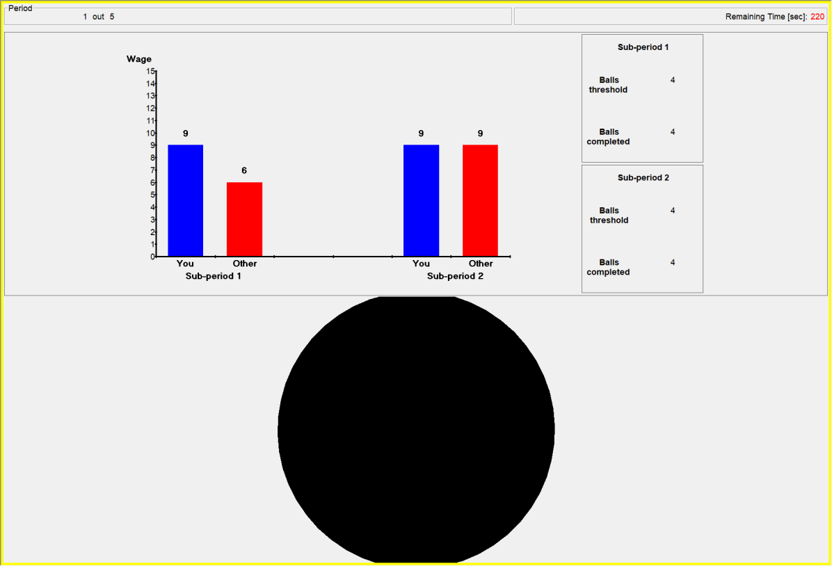
Figure 1: Screenshot of task in sub-period 2 (CatchingUp treatment)

At the start of a period, participants are informed of their wage for the first sub-period a few seconds before the first sub-period starts. During a period, they monitor how their own wage and the wage of their matched partner evolve over the two sub-periods. This information is visualized through one graph exhibiting one’s own wages and the wages of the other participant over the period up to the current sub-period. That is, participants see the wages in the current sub-period, and if they are in the second sub-period, they also see the wages from the previous sub-period. In addition to providing a screenshot of the task, Figure 1 also shows how participants observe the evolution of wages in sub-period 2. The screen presents the wage information from the first sub-period on the left part of the graph, and from the second sub-period on the right part of the graph. Participants have an additional minute to rest in between the two sub-periods. A few seconds before the second sub-period starts, they are informed about any wage changes that occur between the sub-periods.

The participants are paid the two wages of a period—one for each of the two sub-periods—if and only if they complete the task in both sub-periods. A third of each wage that they earn during the two sub-periods is taken from them and placed in a joint account. That is, the joint account contains a third of the two wages of one participant, and a third of the two wages of the other participant.

At the end of each period, the two participants individually propose how to distribute the money contained in the joint account, which has been collected from their wages for the two sub-periods. This is implemented through a dictator game with role uncertainty. That is, one of the two choices is randomly chosen to count. The money in the joint account always amounts to 11 Euro. Participants can keep the entire joint account for themselves, transfer its content to the other participant, or chose any in-between allocation in increments of 10 cents. To further distinguish the different periods, participants then take a two-minute break before the next period starts. At the end of the experiment, one of the two participants’ choices from one period is randomly chosen to count for payment.

We chose a within-subject design in order to increase statistical power (Bellemare et al.,, 2016). We employ five treatments that we implement for each participant over the five periods. The treatments vary the wage changes faced by participants between the first and second sub-period of a period. A participant is always in the role of either the High Earner or the Low Earner. Participants are not informed that they stay in their role. In the first role (High Earner), a participant always experiences advantageous income inequality over the period. That is, the sum of the two wages in a period is always 18 Euro. Similarly, the Low Earner always faces disadvantageous income inequality over the period—the sum of the two wages is always 15 Euro. This allows us to maintain the same income inequality over the period in all treatments, such that income inequality cannot explain any treatment differences.

Table 1: Overview of Income Trends in Treatments

Treatment High Earner / Low Earner Stable IntraDecrease (Intra-personal decrease for Low and High Earners) IntraIncrease (Intra-personal increase for Low and High Earners) IntraInterChange (Intra- and inter-personal decrease for Low Earners) CatchingUp (Inter-personal decrease for High Earners) • Wages are indicated on the vertical axis in Euro, and the two sub-periods of a period are indicated on the horizontal axis. Income inequality is constant over the period: income is 15 Euro for the Low Earner and 18 Euro for the High Earner.

Table 1 details the wages of Low Earners and High Earners over the two sub-periods in the five treatments. The order of treatments is randomized. As we are interested in studying individual responses to absolute and relative wage decreases, we designed the following treatments varying wages changes. While those treatments do not cover all possible wage changes, they do provide several types of declining wages, as well as one set of stable wage and one increasing wage profile.

In Stable, the wage of each participant remains constant in the two sub-periods. In IntraDecrease and IntraIncrease, both participants face either an absolute wage increase or decrease. This allows us to study the effects of intra-personal wage changes. In IntraInterChange, the Low Earner experiences a wage decrease while the High-Earner experiences a wage increase. The wage changes are therefore both absolute and relative for the two participants. In CatchingUp, the wage of the Low Earner increases, while the wage of the High Earner is constant. That is, the High Earner encounters a relative wage decrease—the Low Earner is “catching up” with the High Earner.

Before starting the experiment, the experimenter reads the instructions aloud and participants are provided with a written copy detailing all steps of the experiment. After reading the instructions, participants complete comprehension questions, and help is provided if needed. They also go through a practice period, which is a shorter version of a real period, so that they become familiar with the proceedings of a period. This practice period includes the task and the redistribution decision, but does not count for payment. In it, each participant has the same wage, which stays constant of the two sub-periods. Participants are informed that they are paired with a participant in the same laboratory session in each period.

We designed the experiment using the software z-Tree (Fischbacher,, 2007). It was conducted at the BEElab (Behavioural and Experimental Economics Laboratory) of Maastricht University in May-October 2019. Our sample consists of 294 participants recruited over 16 sessions via the online recruitment software ORSEE (Greiner,, 2015). The experiment lasted for about 90 minutes and participants earned 16.50 Euro on average.

3 The Model

We build our model by combining (i) the inequity aversion model of Bolton and Ockenfels, (2000) (henceforth BO) and (ii) the reference dependence model of Kőszegi and Rabin, (2006) (henceforth KR), in the form employed by DellaVigna et al., (2017), which is loss aversion to previous income. Before we describe the model, transparency requires us to mention that, although we sketched its foundations for advancing pre-experiment predictions in Section 4, we only formalized it after conducting the experiment. Therefore, we do not test this model, but we rather employ it to better organize and enrich our ideas regarding the effect of income trends on redistribution decisions. Importantly, the model predicts that decreasing income trends should only affect the subset of individuals who are sufficiency altruistic (Proposition 2), a proposition that we subsequently use in Section 5.

We consider the following multi-period model with two individuals. In each period, each individual receives an income. We denote by $y_{i}\in\mathbb{R}_{+}$ the final income gained by individual $i$ over all periods, and by $t_{i}\in\mathbb{R}_{+}$ the individual’s final income trend generated by the streams of wages over the periods. In particular, $t_{i}$ takes negative values when the trend is decreasing and positive values otherwise. We assume that the individual has personal concerns, specifically (i) final income over the periods and (ii) final income trend, and social concerns, specifically (iii) relative final income over the periods and (iv) relative final income trend. Formally, individual $i$’s utility consists of four components: (i) material payoff motivation function $u_{i}(y_{i})$, (ii) trend gain-loss function $\mu_{i}(t_{i})$, (iii) relative income motivation function $\sigma_{i}(y_{i},y_{j})$, and (iv) relative trend motivation function $\tau_{i}(t_{i},t_{j})$. We describe the individual’s utility as

$$U_{i}(u_{i},\mu_{i},\sigma_{i},\tau_{i}).$$ (1)

We impose the restriction that (1) is additive and separable and that it satisfies the following assumptions:

A0: $u_{i}(x)$, $\sigma_{i}(x)$ and $\tau_{i}(x)$, are continuous and twice differentiable for all $x$.

A1: $\mu_{i}(t_{i})$ is continuous, differentiable for $t_{i}\neq 0$ with $\mu_{i}(0)=0$, and strictly increasing.

A2: If $z>x>0$, then $\mu(z)+\mu(-z)<\mu(x)+\mu(-x)$.

A3: $\mu_{i}(t_{i})$ is concave for $t_{i}>0$ and convex for $t_{i}<0$.

A4: $\lim_{t\to 0}\frac{\mu^{\prime}(-|t_{i}|)}{\mu^{\prime}_{i}(|t_{i}|)}\equiv\lambda>1$.

A5: $u_{i}(y_{i})$ is increasing and concave in $y_{i}$.

A6: $\sigma_{i}$ is increasing and concave in $y_{i}$ with a maximum at $y_{j}$.

A7: $\tau_{i}$ is increasing and concave in $t_{i}$ with a maximum at $t_{j}$.

We make assumption A0 for mathematical convenience. Assumptions A1–4 recast reference dependence and loss aversion as in KR. Finally, assumption A5–7 are in the spirit of narrow self interests and comparative effect in BO.

In our application, the material payoff motivation function is represented by

$$u_{i}(y_{i})=y_{i}$$

which satisfies A0 and A5. In line with KR and thus with assumption A1–4, we specify the trend gain-loss function as

$$\mu_{i}(t_{i})=\begin{cases}\eta t_{i}&\text{if}\ \ t_{i}<0\\ 0&\text{if}\ \ t_{i}\geq 0\end{cases}$$

with $\eta\in[0,1)$. Next, we write the relative income and trends motivation functions as follows

$$\sigma_{i}(y_{i},y_{j})=\left(y_{i}-\frac{1}{2}(y_{i}+y_{j})\right)^{2}$$

$$\tau_{i}(t_{i},t_{j})=\left(t_{i}-\frac{1}{2}(t_{i}+t_{j})\right)^{2}$$

where we take $\frac{1}{2}(y_{i}+y_{j})$ and $\frac{1}{2}(t_{i}+t_{j})$ to be the reference points, which is similar in form to BO and satisfies assumptions A0 and A5–7. Finally, we consider the following utility specification

$$U_{i}(y_{i},y_{j},t_{i},t_{j})=\begin{cases}a_{i}(y_{i}+\eta t_{i})-b_{i}\left[\left(\frac{1}{2}(y_{i}-y_{j})\right)^{2}+\left(\frac{1}{2}(t_{i}-t_{j})\right)^{2}\right]&\text{if}\ \ t_{i}<0\\ a_{i}y_{i}-b_{i}\left[\left(\frac{1}{2}(y_{i}-y_{j})\right)^{2}+\left(\frac{1}{2}(t_{i}-t_{j})\right)^{2}\right]&\text{if}\ \ t_{i}\geq 0\end{cases}$$ (2)

where $a_{i},b_{i}>0$ are the agent’s sensitivity to personal concerns and social concerns, respectively. We interpret $a_{i}/b_{i}$ as the agent’s type, i.e., the ratio of weights attributed to the personal and social components of the motivation function. Note that our model reduces to a BO-type motivation function when $t_{i}=t_{j}=0$. Furthermore, the first two components of $U_{i}(u_{i},\mu_{i},\sigma_{i},\tau_{i})$ replicate the reference-dependence framework of KR. Specifically, the reference point in one’s own trend is imposed to be zero in $\mu_{i}$, i.e., the individual experiences an extra disutility from his/her own trend being negative, while there is no extra utility from one’s trend being positive. This is similar to DellaVigna et al., (2017), which assumes loss aversion to previous income. Our utility function therefore reduces to a KR-type function when a participant does not care about social comparisons ($b_{i}=0$)

3.1 The Dictator Game

Our experimental design boils down to a Dictator Game at the end of an economy with 2 sub-periods. This is therefore the game that we study here. At end of each sub-periods, each individual receives a wage. Let $W_{i}>0$ be individual $i$’s sum of wages over the two sub-periods. We denote by $\Delta_{i}$ the difference between the wage in the second sub-period and the wage in the first sub-period. In the Dictator Game, individual $i$, who plays the role of the dictator, chooses the share $1-s$ ($0\leq s\leq 1$) of a tax account $T>0$ to give to another individual $j$ who is in the role of the recipient and does not make any decisions ($T$ is independent of everything else). This additional amount modifies the wage in the second sub-period, which affects income levels as well as income trends. In light of our model, the final income of the dictator over the two periods is therefore given by $y_{i}=W_{i}+s$ and the final income trend by $t_{i}=\Delta_{i}+s$. Note that we use the term “final” because we are concerned about the income and the income trend at the very end of the timeframe, i.e., after the redistribution decision. For the recipient, the final income and final income trend are given by $y_{j}=W_{j}+1-s$ and $t_{j}=\Delta_{i}+1-s$. Therefore, the utility function $U_{i}^{D}(y_{i},y_{j},t_{i},t_{j})$ of the dictator takes the form

$$U^{D}_{i}(.)=\begin{cases}a_{i}(W_{i}+sT+\eta(\Delta_{i}+sT))\\ \qquad\quad-b_{i}\left[\left(\frac{1}{2}(W_{i}-W_{j}+2sT-T)\right)^{2}+\left(\frac{1}{2}(\Delta_{i}-\Delta_{j}+2sT-T)\right)^{2}\right]&\text{if}\ \ \Delta_{i}+sT<0\\ a_{i}(W_{i}+sT)\\ \qquad\quad-b_{i}\left[\left(\frac{1}{2}(W_{i}-W_{j}+2sT-T)\right)^{2}+\left(\frac{1}{2}(\Delta_{i}-\Delta_{j}+2sT-T)\right)^{2}\right]&\text{if}\ \ \Delta_{i}+sT\geq 0\end{cases}$$

The thick red curve in Figure 2 panel (a) presents an example of the dictator’s utility function, $U^{D}_{i}$, for our model. In contrast, the dashed black curve in the same panel illustrates the BO-style model, where we remove our trend gain-loss function and our relative trend motivation function. Figure C.1 in Appendix C provides additional examples of $U^{D}_{i}$ for different agent types.

The following proposition provides optimality conditions for $U_{i}^{D}(y_{i},y_{j},t_{i},t_{j})$.

Proposition 1.

Define $\mathbb{H}\equiv W_{i}-W_{j}-2T-3\Delta_{i}-\Delta_{j}$. Then the function $U_{i}^{D}(y_{i},y_{j},t_{i},t_{j})$ is maximized at $s^{*}$ such that:

$$\operatorname*{arg\,max}U_{i}^{D}(y_{i},y_{j},t_{i},t_{j})=\begin{cases}s^{*}=\frac{a_{i}}{b_{i}}\frac{1}{4T}+\frac{1}{2}+\frac{(W_{j}-W_{i})}{4T}+\frac{(\Delta_{j}-\Delta_{i})}{4T}&if\ \frac{a_{i}}{b_{i}}>\mathbb{H}\\ s^{*}=\frac{a_{i}}{b_{i}}\frac{(1+\eta)}{4T}+\frac{1}{2}+\frac{(W_{j}-W_{i})}{4T}+\frac{(\Delta_{j}-\Delta_{i})}{4T}&if\ \frac{a_{i}}{b_{i}}<\frac{\mathbb{H}}{1+\eta}\\ s^{*}=-\frac{\Delta_{i}}{T}&if\ \frac{\mathbb{H}}{1+\eta}\leq\frac{a_{i}}{b_{i}}\leq\mathbb{H}\end{cases}$$

The proof, shown in Appendix C, relies on the fact that $U_{i}^{D}(y_{i},y_{j},t_{i},t_{j})$ is a piecewise function consisting of two concave functions.

The thick red curve in Figure 2 panel (b) depicts an example of the optimal taking choice $s^{*}$ corresponding to $U_{i}^{D}(y_{i},y_{j},t_{i},t_{j})$ when $\Delta_{j}=-5$ and $\Delta_{i}$ varies from $-10$ to $10$. Specifically, when $t_{i}=\Delta_{i}+sT$ is negative, the trend gain-loss component of the model bites and the consequent disutility induces the dictator to keep more for him/herself by choosing a higher $s^{*}$. As $t_{i}=\Delta_{i}+sT$ becomes positive, inequality aversion in trends $\sigma_{i}(t_{i},t_{j})$ decreases $s^{*}$. The dashed black curve represents the BO prediction, which is not affected by variations in trends.

(a) $\Delta_{j}=\Delta_{i}=-5$

(b) $\Delta_{j}=-5$

Figure 2: Examples of $U^{D}_{i}$ and $s^{*}$ for $a_{i}/b_{i}=4$, $W_{i}=10$, $W_{j}=5$, $T=9$, and $\eta=0.8$. The thick line indicates our model predictions and the dashed line indicates BO predictions.

As outlined earlier, the functional form in (2) allows us to express individual heterogeneity through an individual type, which we take as the ratio $a_{i}/b_{i}$. The purely selfish individual is characterized by the limiting case $a_{i}/b_{i}\to\infty$, which implies $s^{*}=1$. At the other extreme, the purely altruistic individual is represented by $a_{i}/b_{i}=0$. However, the value of $s^{*}$ for the altruistic individual depends on relative incomes and trends. Since those two relative terms can be positive or negative, $s^{*}$ can deviate from an equal share. A similar argument applies to any type of non fully selfish individual. The next proposition characterizes corner and interiors solutions in terms of individual types by providing an upper bound $\mathbb{U}$ and a lower bound $\mathbb{L}$.

Proposition 2.

Define $\mathbb{U}\equiv W_{i}-W_{j}+\Delta_{i}-\Delta_{j}+2T$ and $\mathbb{L}\equiv(W_{i}-W_{j}+\Delta_{i}-\Delta_{j}-2T)(1+\eta)^{-1}$. Then,

$$\operatorname*{arg\,max}U_{i}(u_{i},\mu_{i},\sigma_{i},\tau_{i})=\begin{cases}s^{*}=1&if\ \frac{a_{i}}{b_{i}}\geq\mathbb{U}\\ s^{*}=0&if\ \frac{a_{i}}{b_{i}}\leq\mathbb{L}\\ s^{*}\in(0,1)&if\ \mathbb{L}<\frac{a_{i}}{b_{i}}<\mathbb{U}\end{cases}$$

In addition to income inequality aversion, two behavioral phenomena coexists in our model: loss aversion in one’s own trend and inequality aversion in relative trends. The next two propositions disentangle the two separate effects.

Proposition 3.

Suppose $\Delta_{i}=\Delta_{j}$. Then $s^{*}$ (weakly) increases in $[0,1]$ when $\Delta_{i}$ decreases.

The thick red curve in Figure 3 panel (a) illustrates Proposition $3$ with an example of how $s^{*}$ varies when we change an individual’s trend while keeping other factors constant. There is a region where the trend ($t_{i}=\Delta_{i}+sT$) becomes negative and $s^{*}$ increases. As the trend becomes positive, the model reduces to the BO-type model, which is displayed by the dashed black curve. We show in the next proposition that, given any individual trend, a lower relative trend decreases the dictator’s sharing, i.e., $s^{*}$ increases when $\Delta_{j}$ increases.

Proposition 4.

Suppose $\Delta_{i}$ is constant. Then $s^{*}$ (weakly) increases in $[0,1]$ when $\Delta_{j}$ increases.

The thick red curve in Figure 3 panel (b) illustrates Proposition $4$ with an example of $s^{*}$ when we vary the other individual’s trend, keeping everything else constant. In this case, our prediction reduces to the BO prediction when the relative trend is zero. The difference is that the dictator shares less (more) to compensate a negative (positive) relative trend.

(a) $\Delta_{i}=\Delta_{j}$

(b) $\Delta_{i}=0$

Figure 3: An example of $s^{*}$ for $a_{i}/b_{i}=2$ $W_{i}=12$, $W_{j}=10$, $T=11$ and $\eta=0.8$. The thick line indicates our model predictions and the dashed line indicates BO predictions.

4 Hypotheses

We posit that individuals with decreasing incomes experience disutility and take from others to be compensated. Specifically, we assume two forms of disutility: (i) intra-personal disutility created by a negative trend, and (ii) inter-personal disutility created by a negative relative trend. We formalized this idea in Section 3. In this section, we provide hypotheses for each role in the experiment: High and Low Earners. Keep in mind that, before redistribution takes places, High Earners face the same sum of incomes and income inequality over a period in every treatment, and that the same is true for Low Earners.

First, High Earners experience a negative trend IntraDecrease and a negative relative trend in CatchingUp. In contrast, they do not experience a negative trend or negative relative trend Stable, IntraIncrease, and IntraInterChange. In line with Propositions 3 and 4, we predict the following, which does not distinguish between absolute and relative negative trends.

Hypothesis 1.

High Earners give less in IntraDecrease and CatchingUp  than in  Stable, IntraIncrease, and  IntraInterChange.

Second, Low Earners encounter a negative trend in IntraDecrease and a negative absolute and relative trend in IntraInterChange. In contrast, they do not face a negative trend in Stable, IntraIncrease, and CatchingUp. In line with Propositions 3 and 4, we make the following prediction.

Hypothesis 2.

Low Earners give less in IntraInterChange and IntraDecrease than in Stable, IntraIncrease   and CatchingUp.

Low Earners face an absolute and relative negative trend only in IntraInterChange, and at most a decreasing trend in the other treatments. Therefore, consistent with Proposition 4, we also predict the following.

Hypothesis 3.

Low Earners give less in IntraInterChange than in IntraDecrease, Stable, IntraIncrease, and CatchingUp.

Similarly, since Low Earners only experience a negative trend in IntraDecrease, we can make the following prediction, which is consistent with Proposition 4.

Hypothesis 4.

Low Earners give less in IntraInterChange than in IntraDecrease.

5 Estimating the Effect of Decreasing Incomes

We first provide summary statistics regarding the amounts shared in the different treatments. Then we proceed to test the effect of decreasing wages within a period on giving at the end of that period. We make a distinction between the full sample and participants with sufficiently-strong social preferences, whom our framework predicts to be the only ones to become less generous when experiencing decreasing wages (see Proposition 2 in Section 3).

Summary Statistics

Table 2 presents the average amount from the 11-Euro joint account that participants give to the other participant. We provide the data for all participants and then for those participants with sufficiently-strong social preferences, i.e., who give a minimum amount in the baseline treatment with constant wages (Stable). We use a minimum amount of 2 Euro, but the results are robust to using different cutoff points. Overall, mean giving is 1.53 Euro (SD = 2.23 Euro; N = 1,470 observations, 294 participants) or 14% of the joint account for the entire sample, and 4.12 Euro (SD = 1.93 Euro; N = 455 observations, 91 participants) or 37% of the joint account for those with social preferences. High Earners and Low Earners exhibit similar mean giving (for all participants, High Earners give 1.57 Euro (SD = 2.13 Euro; N = 147) and Low Earners give 1.49 (SD = 2.02; N = 147); t-test and Mann-Whitney-Wilcoxon rank test p-values $\geq$ 0.599; the difference is smaller and p-values larger for socially-inclined participants). The giving patterns are more pronounced for participants with social preferences: High Earners are less generous in CatchingUp and perhaps in IntraDecrease; Low Earners are less generous in IntraInterChange.

Compared to dictator games in general, average giving in our experiment is on the lower side of the spectrum found in the literature (see meta-study by Engel, (2011) and comment by Zhang and Ortmann, (2014); average giving in the dictator game is $28.3\%$). Factors present in our study can reduce generosity, namely using a student sample, endowing recipients, repeating the game, dictators earning the money that they can redistribute, and the option of taking money from others, although having deserving recipients who earned the money that the dictator redistributes can increase giving. Moreover, role uncertainty about who will give and who will receive has also been shown to increase pro-sociality in dictator games (Iriberri and Rey-Biel,, 2011).

Amount given All participants Participants with social preferences Treatment High Earners Low Earners High Earners Low Earners Mean (SD) Mean (SD) Mean (SD) Mean (SD) Stable 1.62 1.49 4.74 4.54 (2.35) (2.18) (1.46) (1.60) IntraDecrease 1.57 1.48 3.86 4.14 (2.42) (2.15) (2.17) (1.99) CatchingUp 1.41 1.58 3.61 4.19 (High Earners inter-personal decrease) (2.20) (2.15) (1.98) (1.92) IntraInterChange 1.62 1.42 4.16 3.71 (Low Earners inter- and intra-personal decrease) (2.34) (2.03) (2.01) (1.99) IntraIncrease 1.63 1.45 4.29 3.99 (2.39) (2.13) (1.90) (2.09) $N$ 147 147 48 43 • Note: Participants could give any amount between 0 and 11 Euro from the 11-Euro joint account. The remaining amount was credited to their own account. Participants with social preferences are those exhibiting sufficiently-strong advantageous inequality aversion, i.e., they give at least 2 Euro in the baseline treatment Stable. Table D.1 shows that other cutoff points such as at least 3 Euro, 1 Euro, and 0.25 Euro in Stable provide similar pictures.

Table 2: Summary statistics

Figure 4 shows the cumulative distribution of the amounts given, for High Earners and Low Earners, separately for the entire sample and for those participants with social preferences. There is extensive lower-bound censoring in the full sample—participants give nothing in 56% of decisions—and this censoring mostly vanishes for socially-inclined participants.

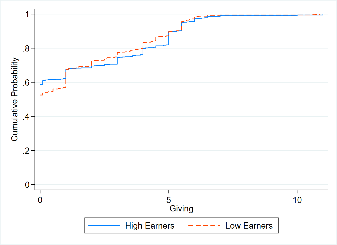
(a) All participants

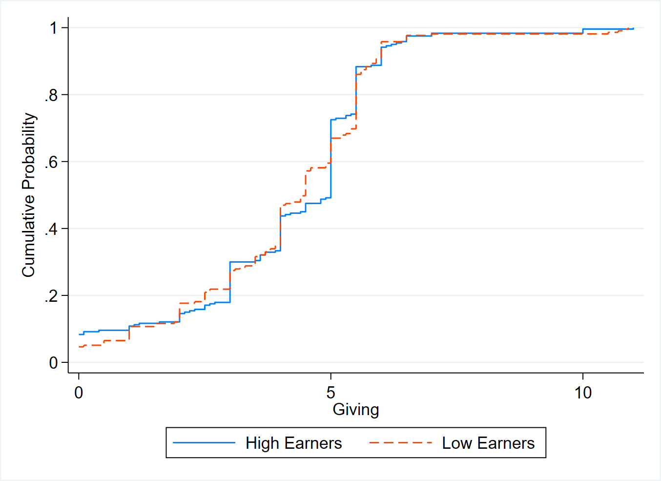
(b) Participants with social preferences

Figure 4: Cumulative distribution functions of giving

Tests

Table 3 shows the estimated effect of the wage decrease treatments on giving. We use Tobit Random Effects regressions (Tobit RE) for the heavily-censored full sample, and Random Effects regressions (RE) for participants with sufficiently-strong social preferences. In Appendix D, Table D.2 shows that results are very similar with Fixed Effects (FE) regressions for participants with sufficiently-strong social preferences, and Table D.3,  D.4, and  D.5 show that the RE results are also very similar if we use alternative cutoff points for defining participants with social preferences (giving at least 3 Euro, 1 Euro, and 0.25 Euro in Stable). Any decrease includes all treatments with decreasing incomes (IntraDecrease and CatchingUp for Higher Earners and IntraDecrease and IntraInterDecrease for Low Earners). Any strictly intra decrease denotes all treatments with only intra-personal decreasing incomes (CatchingUp for High Earners and IntraInterDecrease for Low Earners), and Any inter decrease denotes all treatments with inter-personal decreasing incomes (CatchingUp for High Earners and IntraInterDecrease for Low Earners). Columns 1–6 display the results for all participants, and columns 7–20 for participants with sufficiently-strong social preferences. The results are presented for All Earners or separately for High Earners and Low Earners. We include period dummies, and a dummy for High Earners when we employ all Earners in the regression.

Importantly, for socially-inclined participants, we present the results including and excluding the Stable treatment. This matters because including Stable in the regression could create a spurious negative relationship between the decreasing treatments and Stable. For instance, suppose that participants’ differences in giving choices across treatments simply consist of noise: they randomly give 0 or 2 Euro for every decision. Then, if we compare the other treatments to Stable only for participants with social preferences (defined as those who give at least 2 Euro in Stable where there is no wage trend), those participants will mechanically appear less generous in the other treatments. Reassuringly, our results show that, while excluding Stable qualitatively affects the size of the estimates, it has minor impacts on our conclusions.

To complement this analysis, Table 4 presents Wilcoxon signed-rank tests roughly equivalent to several tests in Table 3. We write roughly because those tests only provide pairwise comparisons of treatments. Although they reduce statistical power, their advantage is to relax the normality of error terms assumption. The conclusions that we can draw from those tests are similar to those using regressions, but the results are not always significant. We indicate in footnotes whenever differences arise.

We make three sets of observations regarding the analyses reported in Table 3. First, when considering High and Low Earners together (columns 1-2 and 7-8), any decrease in income reduces giving at marginally significant levels for the full sample and at highly significant levels for participants with social preferences. For participants with social preferences, the effect amounts to approximately $-0.5$ Euro; relative to their mean giving of 4.12 (SD = 1.93) Euro, this corresponds to 1/4 of a standard deviation. Once we separate any strictly intra-personal decreases and any inter-personal decreases (column 2 and 9-10), we observe that only inter-personal decreases have a significant impact in the full sample and in our robust specification excluding the Stable treatment for participants with social preferences (the effect of any strictly intra-personal decreases is significant under our basic specification). The Wald tests indicate that difference between any strictly intra-personal decreases and any inter-personal decreases is not significant in the full sample, and marginally significant under our preferred robust specification for social participants (just below the 0.05 significance threshold under our basic specification). We provide a first result of the effect of decreasing incomes among all Earners because we believe it informative to provide an aggregate picture, but this first result does not correspond to any specific hypothesis. We write it as follows.

Result 1.

Among all Earners with social preferences, decreasing incomes reduce average giving compared to non-decreasing incomes; inter-personal decreases have a significant effect, which is marginally stronger than that of strictly intra-personal decreases. Decreasing incomes have a marginally significant impact in the full sample.

(1) (2) (3) (4) (5) (6) (7) (8) (9) (10) (11) (12) (13) (14) (15) (16) (17) (18) (19) (20) Tobit RE Tobit RE Tobit RE Tobit RE Tobit RE Tobit RE RE RE RE RE RE RE RE RE RE RE RE RE RE RE All Participants Participants with Social Preferences All Earners High Earners Low Earners All Earners High Earners Low Earners Any decrease $-$0.176^∗ $-$0.304 $-$0.104 $-$0.483^∗∗∗ $-$0.331^∗∗∗ $-$0.636^∗∗∗ $-$0.507^∗∗ $-$0.322^∗∗∗ $-$0.151 (0.105) (0.187) (0.114) (0.117) (0.122) (0.200) (0.210) (0.115) (0.120) Any strictly intra decrease $-$0.055 $-$0.301^∗∗ $-$0.159 (0.133) (0.118) (0.134) Any inter decrease $-$0.295^∗∗ $-$0.660^∗∗∗ $-$0.502^∗∗∗ (0.133) (0.172) (0.166) Wald test p-value 0.142 0.050 0.054 IntraDecrease $-$0.170 0.012 $-$0.492^∗∗∗ $-$0.367^∗ $-$0.094 0.066 (0.235) (0.143) (0.182) (0.203) (0.135) (0.167) CatchingUp $-$0.437^∗ $-$0.781^∗∗ $-$0.653^∗∗ (0.236) (0.308) (0.308) IntraInterDecrease $-$0.219 $-$0.551^∗∗∗ $-$0.376^∗∗ $-$0.527^∗∗∗ $-$0.398^∗∗ (0.144) (0.181) (0.164) (0.182) (0.168) Wald test p-value 0.355 0.188 0.352 0.349 0.038 0.048 Constant $-$0.446 $-$0.441^∗∗∗ $-$0.902^∗ $-$0.909^∗ 0.194 0.208 4.484^∗∗∗ 4.199^∗∗∗ 4.491^∗∗∗ 4.208^∗∗∗ 4.556^∗∗∗ 4.243^∗∗∗ 4.547^∗∗∗ 4.231^∗∗∗ 4.361^∗∗∗ 4.133^∗∗∗ 4.398^∗∗∗ 4.187^∗∗∗ 4.378^∗∗∗ 4.209^∗∗∗ (0.426) (0.425) (0.520) (0.519) (0.399) (0.399) (0.202) (0.248) (0.201) (0.246) (0.213) (0.272) (0.215) (0.276) (0.247) (0.271) (0.246) (0.268) (0.248) (0.271) Without Stable ✓ ✓ ✓ ✓ ✓ ✓ ✓ Period dummies ✓ ✓ ✓ ✓ ✓ ✓ ✓ ✓ ✓ ✓ ✓ ✓ ✓ ✓ ✓ ✓ ✓ ✓ ✓ ✓ High Earners dummy ✓ ✓ ✓ ✓ ✓ ✓ $N$ 1470 1470 735 735 735 735 455 364 455 364 240 192 240 192 215 172 215 172 215 172 • Note: Giving is indicated in Euro. Participants with social preferences are those exhibiting sufficiently-strong advantageous inequality aversion, i.e., they give at least 2 Euro in the baseline treatment Stable. Table D.3,  D.4, and  D.5 show that the results are very similar if we use alternative cutoff points for defining participants with social preferences (giving at least 3 Euro, 1 Euro, and 0.25 Euro in Stable). Any decrease denotes IntraDecrease and CatchingUp for High Earners, and IntraDecrease and IntraInterDecrease for Low Earners. Any strictly intra decrease denotes IntraDecrease for High and Low Earners. Any inter decrease denotes CatchingUp for High Earners and IntraInterDecrease for Low Earners. All treatments are included in the regression, except when we indicate that we remove the Stable treatment. We indicate p-values from Wald test on the equality of the coefficients of Any strictly intra decrease and Any inter decrease, and on the equality of IntraInterDecrease and IntraDecrease or CatchingUp. The coefficient of the High Earners dummy is always far from the 10% significance threshold. Table D.2 also shows that results are very similar with Fixed Effects regressions for participants with sufficiently-strong social preferences. Standard errors are in parentheses. ^∗ p$<$0.10, ^∗∗ p$<$0.05, ^∗∗∗ p$<$0.01.

Table 3: Regression tests of the effect of decreasing wages on giving

(1) (3) (4) (5) (6) (7) (8) (9) All Participants Social Participants Stable IntraIncrease OtherNoDecrease IntraDecrease Stable IntraIncrease OtherNoDecrease IntraDecrease All Earners IntraDecrease 0.042 0.268 0.050 $<$0.001 0.643 0.245 OtherDecrease 0.058 0.147 0.026 $<$0.001 0.014 0.008 N 294 294 294 91 91 91 High Earners IntraDecrease 0.145 0.172 0.198 0.001 0.216 0.268 CatchingUp 0.045 0.064 0.053 0.455 $<$0.001 0.032 0.087 0.309 N 147 147 147 147 48 48 48 48 Low Earners IntraDecrease 0.173 0.813 0.140 0.004 0.536 0.618 IntraInterDecrease 0.439 0.727 0.202 0.968 0.001 0.176 0.037 0.241 N 147 147 147 147 43 43 43 43 • Note: OtherDecrease denotes CatchingUp for High Earners and IntraInterDecrease for Low Earners; OtherNoDecrease denotes IntraInterDecrease for High Earners and CatchingUp for Low Earners.

Table 4: Wilcoxon signed-rank tests of the effect of decreasing wages on giving

Second, among socially-inclined High Earners (columns 11–14), the intra-personal (IntraDecrease) and the inter-personal (CatchingUp) decreases in income reduce average giving, at marginal and significant levels, respectively, under our preferred robust specification without Stable. Although the effect of inter-personal decrease (approx. $-0.7$ Euro) is qualitatively larger than that of the intra-personal decrease (approx. $-0.4$ Euro), the Wald tests show that the two are statistically indistinguishable. Furthermore, only the effect of inter-personal decrease is marginally significant with the full sample (column 4). The evidence is in line with Hypothesis 1 for participants with social preferences, but not for the full sample. We therefore write our second result as follows.

Result 2.

Among High Earners with social preferences, decreasing incomes reduce average giving compared to non-decreasing incomes; inter- (CatchingUp) and intra-personal (IntraDecrease) decreases have significant and marginally significant effects, respectively, but the two are statistically indistinguishable. Only the effect of inter-personal decreases is marginally detectable in the full sample.

Third, among Low Earners with social preferences (columns 15–18), the joint intra- and inter-personal decrease in incomes (IntraInterDecrease) significantly reduces average giving (approx. $-0.4$ Euro), but the point estimate of intra-personal decrease (IntraDecrease) is nearing 0 and not significant. The table’s Wald test shows that the effect of the joint intra- and inter-personal decrease is significantly larger than the the intra-personal effect. The joint intra- and inter-personal decrease is also significantly larger than all other schemes bundled together (columns 19-20). Moreover, similarly as for High Earners, no effect of any of the two types of income decreases has an effect on Low Earners in the full sample. Overall, for Low Earners with social preferences, the evidence goes against Hypothesis 2, which ascertains that both types of decreases would reduce giving. However, the evidence falls in line with Hypotheses 3 and 4, which predict that the joint intra- and inter-personal decrease would lower giving and that its effect would be larger than that of the intra-personal decrease. The full sample supports none of those three hypotheses. We thus write our third result as follows.

Result 3.

Among Low Earners with social preferences, the joint intra- and inter-personal income decrease (IntraInterDecrease) significantly reduces average giving compared to non-decreasing incomes, and the intra-personal decrease (IntraDecrease) does not; the effect of the first is significantly larger than that of the second. No effect is detectable in the full sample.

To sum up, although income inequality over a period is the same in each treatment, we find strong evidence of a negative effect of decreasing incomes within a period on giving among participants with social preferences. This is the case for all Earners joined together, and, when we consider the different roles in the experiment separately, for High and Low Earners evaluated separately. Overall, the evidence is strong for inter-personal decreases rendering participants more selfish and weak for intra-personal decreases. However, the difference between the two is itself limited: the inter-personal decrease is stronger than the intra-personal decrease at marginal significance levels for all Earners evaluated together, and right below significance levels for Low Earners. For the sample as a whole, there is limited (marginally significant) evidence for the negative effect of decreasing incomes on giving.

Evidence that an Increasing Relative Income Trend does not Increase Sharing

(1) (2) (3) RE RE RE All Participants Participants with Social Preferences High Earners High Earners IntraInterDecrease $-0.044$ $-0.365^{*}$ $-0.150$ (0.108) (0.191) (0.198) Constant 1.920 4.828 4.550 (0.216) (0.241) (0.323) Baseline is IntraDecrease & Stable ✓ ✓ Baseline is IntraDecrease alone ✓ Period dummies ✓ ✓ ✓ $N$ 441 144 96 • Note: Giving is indicated in Euro. The treatments included in the regression are IntraInterDecrease and the baseline treatment(s) indicated at the bottom of the table. Standard errors are in parentheses. ^∗ p$<$0.10, ^∗∗ p$<$0.05, ^∗∗∗ p$<$0.01.

Table 5: Tests of the effect of increasing relative wages on giving for High Earners, excluding treatments with decreasing wages

We did not make a hypothesis about how a positive relative income trend might affect generosity. Nevertheless, our formal model differs with our original intuition on this matter. Specifically, through Proposition 4, it predicts, if anything, a positive effect. We evaluate this possibility by using treatment IntraInterChange, where High Earners experience a decreasing relative trend. We compare their sharing behavior in IntraInterChange relative to IntraIncrease and Stable. Table 5 shows the analyses, first for all High Earners and second for socially-inclined High Earners, without and then with removing the Stable treatment for robustness. Overall, we find no evidence that a positive relative trend increases sharing. This gives us an additional fourth result, which does not correspond to a hypothesis.

Result 4.

Among all High Earners and among High Earners with social preferences, the relative increase in incomes (IntraInterDecrease) does not significantly alter average giving compared to other non-decreasing incomes.

Evidence that Order Effects Do not Drive our Results

(1) (2) (3) (4) (5) (6) (7) (8) RE RE RE RE RE RE RE RE Participants with Social Preferences All Earners High Earners Low Earners Period(s) 1-2 1-2 1-2 Any decrease $-$0.832^∗∗∗ $-$0.560^∗∗ $-$1.033^∗∗ $-$0.692^∗∗ $-$0.556^∗ $-$0.456 (0.275) (0.265) (0.457) (0.284) (0.297) (0.385) Any strictly intra decrease -0.340 -0.104 (0.309) (0.381) Any inter decrease $-$1.136^∗∗∗ $-$0.812^∗∗∗ (0.367) (0.306) Wald test p-value 0.075 0.104 Any decrease in 1 period dummy 0.324 0.250 0.293 0.197 0.470 0.333 0.155 0.206 (0.348) (0.432) (0.350) (0.439) (0.471) (0.562) (0.513) (0.629) Constant 4.580^∗∗∗ 4.245^∗∗∗ 4.569^∗∗∗ 4.229^∗∗∗ 4.536^∗∗∗ 4.263^∗∗∗ 4.396^∗∗∗ 4.156^∗∗∗ (0.203) (0.264) (0.202) (0.260) (0.221) (0.284) (0.313) (0.389) Without Stable ✓ ✓ ✓ ✓ Period dummies ✓ ✓ ✓ ✓ ✓ ✓ ✓ ✓ High Earners dummy ✓ ✓ ✓ ✓ $N$ 182 132 182 132 96 69 86 63 • Note: Note: Giving is indicated in Euro. Any decrease denotes IntraDecrease and CatchingUp for High Earners, and IntraDecrease and IntraInterDecrease for Low Earners. Any strictly intra decrease denotes IntraDecrease for High and Low Earners. Any inter decrease denotes CatchingUp for High Earners and IntraInterDecrease for Low Earners. All treatments are included in the regression, except when we indicate that we remove the Stable treatment. We indicate p-values from Wald test on the equality of the coefficients of Any strictly intra decrease and Any inter decrease. Standard errors are in parentheses. ^∗ p$<$0.10, ^∗∗ p$<$0.05, ^∗∗∗ p$<$0.01.

Table 6: Tests of the effect of decreasing wages on giving, in first two periods while controlling for possible order effect of starting with a decreasing income treatment

We provide evidence that order effects do not drive our results by re-running the regressions from Table 3 concerning the effect of any decrease in income as well as any strictly intra decrease and any inter decrease for participants with social preferences, but this time only using the first two periods and including a dummy for facing a treatment with any income decrease in the first period. Table 6 shows the estimates for High and Low Earners together (columns 1–4), High Earners (column 5-6), and Low Earners (column 7-8). Keeping in mind the lower statistical power, the point estimates and significance levels are similar as for the corresponding Table 3 estimations; the dummy for starting with any decreasing income is never significant.

Evidence that First-Period Experience Does not Stop Effect of Decreasing Wages

We show that having some experience with the experiment, in the form of going through the first period, does not stop participants’ reaction to decreasing wages in the next periods. Table 7 reproduces basic regressions from Table 3 for social participants, but adding a term for the interaction between the first period and Any decrease. We do not distinguish between the two types of decreases to avoid diluting statistical power. The table shows that the negative effect of any decrease is not restricted to the first period as the coefficient of any decrease is significant. Furthermore, the interaction term between the first period and any decrease is negative—suggesting a possible greater impact in the first period—but not significant.

(1) (2) (3) (4) (5) (6) RE RE RE RE RE RE Participants with Social Preferences All Earners High Earners Low Earners Any decrease $-$0.365^∗∗∗ $-$0.259^∗∗ $-$0.511^∗∗∗ $-$0.407^∗∗ $-$0.217^∗∗ $-$0.103 (0.100) (0.115) (0.160) (0.190) (0.103) (0.112) Any decrease $\times$ 1 period $-$0.610 $-$0.381 $-$0.745 $-$0.553 $-$0.497 $-$0.258 (0.421) (0.442) (0.771) (0.788) (0.468) (0.503) Constant 4.647^∗∗∗ 4.334^∗∗∗ 4.723^∗∗∗ 4.402^∗∗∗ 4.534^∗∗∗ 4.257^∗∗∗ (0.224) (0.276) (0.250) (0.311) (0.305) (0.349) Without Stable ✓ ✓ ✓ Period dummies ✓ ✓ ✓ ✓ ✓ ✓ High Earners dummy ✓ ✓ $N$ 455 364 240 192 215 172 • Note: Giving is indicated in Euro. Any decrease denotes IntraDecrease and CatchingUp for High Earners, and IntraDecrease and IntraInterDecrease for Low Earners. All treatments are included in the regression, except when we indicate that we remove the Stable treatment. Standard errors are in parentheses. ^∗ p$<$0.10, ^∗∗ p$<$0.05, ^∗∗∗ p$<$0.01.

Table 7: Tests of the effect of decreasing wages on giving, adding a dummy for the first encounter with decreasing wages

Evidence that Misunderstandings do not Drive our Results

Our results are robust to dropping the rare individuals who give almost everything during a period (i.e., $\geq$ 9 Euro from the 11-Euro joint account)—resulting in a greater income for the participant they are matched with than for themselves—because this might indicate that they misunderstood the instructions (alternatively, those participants could simply be very generous). Appendix Table D.6 reproduces some of the regressions from Table 3 for participants with social preferences, but excluding the 2 socially-inclined participants giving 9 Euro or more in at least one period. The results are very similar in terms of significance levels. The exception is that, for all Earners, Wald tests indicate that the difference between any inter decrease and any strict intra decrease is no longer marginally significant (columns 3-4).

6 Conclusion

In this study, we conducted an experiment designed to identify how income decreases causally affect redistribution behavior. Based on the literature on reference dependence, loss aversion, and inequality aversion, we hypothesized that individuals become more selfish when they experience a negative absolute or relative income trend. In the full sample, we found evidence that individuals indeed share less with others after experiencing decreasing incomes, but the effect is only significant at marginal levels.

However, since we study the effect of aversion to decreasing income trends on generosity, we should only expect to observe effects for those individuals who are also inequity averse in outcomes. That is, those who are already fully selfish cannot be made more selfish by manipulating income trends. We indeed found that, for those socially-inclined individuals, a negative income trend reduces generosity, this time at highly significant levels, and independently of the specific cutoff that we employ to define those participants. When we conduct separate analyses by role in the experiment, the effect is significant for those participants who earn relatively more, but, in our robust specification, it is not for those who earn relatively less. Furthermore, inter-personal decreases significantly reduce the generosity of participants, and strictly intra-personal decreases generally do not lower generosity significantly. On the whole, inter-personal decreases appear to have a stronger effect than intra-personal decreases, but the difference is only marginally significant, so that we cannot clearly distinguish the two effects.

Our model can be seen as a first step towards a multi-period extension of Bolton and Ockenfels, (2000), which, in the words of its authors “is a theory of “local behavior” in the sense that it explains stationary patterns […] over a short time span in a constant frame.” Specifically, we incorporate inequality aversion in income as well as inequality aversion in income trends. In the fashion of Kőszegi and Rabin, (2006), we also assume that individuals are averse to their own trend being negative. Our model reduces to a Bolton and Ockenfels, (2000) inequality-aversion model when individuals experience the same positive trends and to a Kőszegi and Rabin, (2006) reference-dependence model when individuals experience the same negative trends and income levels. When income trends diverge, our theory differs from Bolton and Ockenfels, (2000) in that it prescribes a behavior that we observe in the data: a negative relative trend induces more selfishness. For the purpose of this paper, we apply our theory to a dictator game, but natural extensions are to study how income trends may affect behavior in other settings such as bargaining problems, risky decisions, and consumer decisions.

The effect of decreasing incomes on generosity that we report also poses interesting possibilities for future research in domains where social preferences are at play. Redistributive policies aiming to close earnings gaps between groups—such as between ethnic minorities vs. whites, and men vs. women—can be met with more resistance by members of the traditionally better off group who are averse to relative income trends inequality and compare their trends to that of the other groups. Aversion to a negative absolute trend can increase the rich’s opposition to and the poor’s support for fiscal stimuli with redistributive aspects during economic downturns. In the workplace, trend-inequality averse workers might react badly—becoming less productive, less cooperative, engaging in sabotage—when their co-workers face relatively better income profiles over the years.

See pages 1 of Instructions_IncomeTrajectories.pdf

See pages 2- of Instructions_IncomeTrajectories.pdf

Appendix B Screenshots

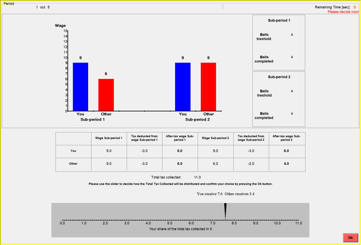
Figure B.1: Screenshot of redistribution stage (CatchingUp

treatment)

Appendix C Additional Information about the Model

Graphical examples of the dictator’ utility function

Figure C.1 presents examples of a dictator’s utility, $U^{D}_{i}$, for different agent types ($a_{i}/b_{i}$).

Figure C.1: Examples of $U_{i}^{D}$ when $X_{1}=10,X_{2}=15,T=9,\Delta_{i}=-6,\Delta_{j}=-10$, and $\eta=0.8$. Thick, dashed, and dotted curves represent agent types ($a_{i}/b_{i}$) $6$, $2$ and $1$.

Proof of Proposition 1: Let $\overline{U}_{i}(y_{i},y_{j},t_{i},t_{j})$ and $\hat{U}_{i}(y_{i},y_{j},t_{i},t_{j})$ denote the two piece-wise components of the dictator’s utility function $U_{i}^{D}(y_{i},y_{j},t_{i},t_{j})$. That is:

$$\hat{U}_{i}(.)=a_{i}(W_{i}+sT+\eta(\Delta_{i}+sT))-b_{i}\left[\left(\frac{1}{2}(W_{i}-W_{j}+2sT-T)\right)^{2}+\left(\frac{1}{2}(\Delta_{i}-\Delta_{j}+2sT-T)\right)^{2}\right]$$

$$\overline{U}_{i}(.)=a_{i}(W_{i}+sT)-b_{i}\left[\left(\frac{1}{2}(W_{i}-W_{j}+2sT-T)\right)^{2}+\left(\frac{1}{2}(\Delta_{i}-\Delta_{j}+2sT-T)\right)^{2}\right]$$

Note that $\overline{U}_{i}(.)$ and $\hat{U}_{i}(.)$ are both continuous and concave with unique maxima at

$$\operatorname*{arg\,max}\overline{U}_{i}(y_{i},y_{j},t_{i},t_{j})=\frac{a_{i}}{b_{i}}\frac{1}{4T}+\frac{1}{2}+\frac{(X_{2}-X_{1})}{4T}+\frac{(\Delta_{j}-\Delta_{i})}{4T}$$

and

$$\operatorname*{arg\,max}\hat{U}_{i}(y_{i},y_{j},t_{i},t_{j})=\frac{a_{i}}{b_{i}}\frac{(1+\eta)}{4T}+\frac{1}{2}+\frac{(X_{2}-X_{1})}{4T}+\frac{(\Delta_{j}-\Delta_{i})}{4T}$$

Also note that the piecewise function $U_{i}^{D}(y_{i},y_{j},t_{i},t_{j})$ has a non differentiable point at $\overline{s}\equiv-\frac{\Delta_{i}}{T}$. Because $\hat{U}_{i}^{\prime}(\overline{s})>\overline{U}_{i}^{\prime}(\overline{s})$, it holds that $U_{i}^{D}(y_{i},y_{j},t_{i},t_{j})$ is a concave function as well and thus has a unique maximum. We consider the following three cases:

Case (i)

$\operatorname*{arg\,max}\overline{U}_{i}\in[\overline{s},\infty)$. Note that, by definition of $U^{D}_{i}$, for all $s<\overline{s}$ it holds that $\overline{U}_{i}(s)>\hat{U}_{i}(s)=U^{D}_{i}(s)$. It follows that $\operatorname*{arg\,max}\overline{U}_{i}=\operatorname*{arg\,max}U^{D}_{i}$ whenever $s\geq\overline{s}$. Recall that, by assumption, $\operatorname*{arg\,max}\overline{U}_{i}\geq\overline{s}$, that is,

$$\frac{a_{i}}{b_{i}}\frac{1}{4T}+\frac{1}{2}+\frac{(X_{2}-X_{1})}{4T}+\frac{(\Delta_{j}-\Delta_{i})}{4T}\geq-\frac{\Delta_{i}}{T}\Longleftrightarrow$$

$$\frac{a_{i}}{b_{i}}\geq W_{i}-W_{j}-2T-3\Delta_{i}-\Delta_{j}$$

Case (ii)

$\operatorname*{arg\,max}\hat{U}_{i}\in(-\infty,\overline{s}]$. Note that, by definition of $U^{D}_{i}$, for all $s>\overline{s}$, it holds that $\hat{U}_{i}(s)>\overline{U}_{i}(s)=U^{D}_{i}(s)$. It immediately follows that $\operatorname*{arg\,max}\hat{U}_{i}=\operatorname*{arg\,max}U^{D}_{i}$ whenever $s\leq\overline{s}$. Recall that, by assumption, $\operatorname*{arg\,max}\overline{U}_{i}\leq\overline{s}$, that is,

$$\frac{a_{i}}{b_{i}}\frac{(1+\eta)}{4T}+\frac{1}{2}+\frac{(X_{2}-X_{1})}{4T}+\frac{(\Delta_{j}-\Delta_{i})}{4T}\leq-\frac{\Delta_{i}}{T}\Longleftrightarrow$$

$$\frac{a_{i}}{b_{i}}\leq\frac{W_{i}-W_{j}-2T-3\Delta_{i}-\Delta_{j}}{1+\eta}$$

Case (iii)

$\operatorname*{arg\,max}\hat{U}_{i}\notin(-\infty,\overline{s})$ and $\operatorname*{arg\,max}\overline{U}_{i}\notin[\overline{s},\infty)$. Since $\hat{U}_{i}$ and $\overline{U}_{i}$ are defined in $U^{D}_{i}$ respectively for $s<\overline{s}$ and $s\geq\overline{s}$, it follows that $\operatorname*{arg\,max}U^{D}_{i}=\overline{s}$. Finally, note that, we are in the case such that $\operatorname*{arg\,max}\hat{U}_{i}>\overline{s}$ and $\operatorname*{arg\,max}\overline{U}_{i}<\overline{s}$. Thus it follows that

$$\frac{a_{i}}{b_{i}}\frac{(1+\eta)}{4T}+\frac{1}{2}+\frac{(X_{2}-X_{1})}{4T}+\frac{(\Delta_{j}-\Delta_{i})}{4T}>-\frac{\Delta_{i}}{T}\Longleftrightarrow$$

$$\frac{a_{i}}{b_{i}}>\frac{W_{i}-W_{j}-2T-3\Delta_{i}-\Delta_{j}}{1+\eta}$$

and

$$\frac{a_{i}}{b_{i}}\frac{1}{4T}+\frac{1}{2}+\frac{(X_{2}-X_{1})}{4T}+\frac{(\Delta_{j}-\Delta_{i})}{4T}<-\frac{\Delta_{i}}{T}\Longleftrightarrow$$

$$\frac{a_{i}}{b_{i}}<W_{i}-W_{j}-2T-3\Delta_{i}-\Delta_{j}$$

Cases (i), (ii), and (iii) together prove the proposition. $\hfill\blacksquare$

Proof of Proposition 2: Assume that $\frac{a_{i}}{b_{i}}\geq\mathbb{U}$. Taking $\mathbb{U}>\mathbb{H}$ together with Proposition 1, it holds that

$$\operatorname*{arg\,max}U_{i}^{D}=s^{*}=\frac{a_{i}}{b_{i}}\frac{1}{4T}+\frac{1}{2}+\frac{(X_{2}-X_{1})}{4T}+\frac{(\Delta_{j}-\Delta_{i})}{4T}$$

To obtain a contradiction, suppose that $s^{*}<1$. This implies that

$$\frac{a_{i}}{b_{i}}\frac{1}{4T}+\frac{1}{2}+\frac{(X_{2}-X_{1})}{4T}+\frac{(\Delta_{j}-\Delta_{i})}{4T}<1\Longleftrightarrow$$

$$\frac{a_{i}}{b_{i}}>W_{i}-W_{j}+\Delta_{i}-\Delta_{j}+2T=\mathbb{U}$$

which is not possible because of the assumption. Thus, for $\frac{a_{i}}{b_{i}}\geq\mathbb{U}$, we know that $s^{*}=1$.

Next, let’s assume that $\frac{a_{i}}{b_{i}}\leq\mathbb{L}$. We consider two cases: $\Delta_{1}\leq 0$ and $\Delta_{i}>0$. In the former case, it holds that $\mathbb{L}\leq\mathbb{H}(1+\eta)^{-1}$. Therefore, by Proposition 1, it also holds that

$$\operatorname*{arg\,max}U_{i}^{D}=s^{*}=\frac{a_{i}}{b_{i}}\frac{1+\eta}{4T}+\frac{1}{2}+\frac{(X_{2}-X_{1})}{4T}+\frac{(\Delta_{j}-\Delta_{i})}{4T}$$

To obtain a contradiction, let’s assume that $s^{*}>0$. It follows that

$$\frac{a_{i}}{b_{i}}\frac{1+\eta}{4T}+\frac{1}{2}+\frac{(X_{2}-X_{1})}{4T}+\frac{(\Delta_{j}-\Delta_{i})}{4T}>0\Longleftrightarrow$$

$$\frac{a_{i}}{b_{i}}>(W_{i}-W_{j}+\Delta_{i}-\Delta_{j}+2T)(1+\eta)^{-1}=\mathbb{U}>\mathbb{L}$$

which is not possible because of the assumption. In the latter case, it holds that $\mathbb{L}>\mathbb{H}(1+\eta)^{-1}$, which corresponds to the remaining case

$$\operatorname*{arg\,max}U_{i}^{D}=s^{*}=\frac{-\Delta_{i}}{T}$$

Since in this case $\Delta_{i}>0$, $s^{*}$ can never be strictly positive. Finally, given the above, it is straightforward to show that the intermediate case yields $s^{*}\in(0,1)$. $\hfill\blacksquare$

Proof of Proposition 3: Recall that by Proposition 1, $s^{*}$ depends on the agent type $a_{i}/b_{i}$. For the high and low type ($a_{i}/b_{i}>\mathbb{H}$,$a_{i}/b_{i}<\mathbb{H}/(1+\eta)$), the value of $s^{*}$ doe not depend on $\Delta_{i}$ whenever $\Delta_{i}=\Delta_{j}$. For the intermediate case, it holds that $\frac{\partial s^{*}}{\partial\Delta_{i}}<0$. $\hfill\blacksquare$

Proof of Proposition 4: For the high and low type ($a_{i}/b_{i}>\mathbb{H}$,$a_{i}/b_{i}<\mathbb{H}/(1+\eta)$), it holds that $\frac{\partial s^{*}}{\partial\Delta_{i}}>0$. For the intermediate case, the value of $s^{*}$ does not depends on $\Delta_{j}$. $\hfill\blacksquare$

Appendix D Additional Tables

Amount given, according to social preferences cutoff (minimum giving in Stable) $\geq$3 Euro $\geq$1 Euro $\geq$0.25 Euro Treatment High Earners Low Earners High Earners Low Earners High Earners Low Earners Mean (SD) Mean (SD) Mean (SD) Mean (SD) Mean (SD) Stable 4.98 4.91 4.16 3.48 4.09 3.21 (1.29) (1.40) (1.91) (2.09) (1.96) (2.17) IntraDecrease 4.10 4.65 3.43 3.21 3.38 2.97 (2.08) (1.62) (2.33) (2.25) (2.34) (2.28) IntraInterChange 4.36 4.10 3.65 2.97 3.60 2.75 (1.94) (1.85) (2.22) (2.09) (2.23) (2.12) CatchingUp 3.78 4.55 3.19 3.38 3.15 3.11 (1.94) (1.75) (2.10) (2.10) (2.10) (2.18) IntraIncrease 4.59 4.38 3.77 3.16 3.72 2.93 (1.66) (1.92) (2.17) (2.23) (2.18) (2.26) $N$ 44 37 57 62 58 68 • Note: Participants could give any amount between 0 and 11 Euro from the 11-Euro joint account. The remaining amount was credited to their own account. Participants with social preferences are those exhibiting sufficiently-strong advantageous inequality aversion, i.e., they give at least the amount of the cutoff in the baseline treatment Stable. The main text uses 2 Euro as the cutoff and we present here descriptive statistics for the alternative cutoffs 3 Euro, 1 Euro, and 0.25 Euro.

Table D.1: Summary statistics with different cutoffs to determine participants with sufficiently-strong social preferences

(1) (2) (3) (4) (5) (6) (7) (8) (9) (10) (11) (12) (13) (14) FE FE FE FE FE FE FE FE FE FE FE FE FE FE Participants with Social Preferences All Earners High Earners Low Earners Any decrease $-$0.483^∗∗∗ $-$0.332^∗∗∗ $-$0.636^∗∗∗ $-$0.509^∗∗ $-$0.322^∗∗∗ $-$0.153 (0.117) (0.122) (0.200) (0.211) (0.115) (0.120) Any strictly intra decrease $-$0.301^∗∗ $-$0.160 (0.118) (0.134) Any inter decrease $-$0.660^∗∗∗ $-$0.502^∗∗∗ (0.172) (0.166) Wald test p-value 0.053 0.058 IntraDecrease $-$0.492^∗∗∗ $-$0.367^∗ $-$0.094 0.064 (0.182) (0.203) (0.135) (0.167) CatchingUp $-$0.781^∗∗ $-$0.657^∗∗ (0.308) (0.310) IntraInterDecrease $-$0.551^∗∗∗ $-$0.377^∗∗ $-$0.527^∗∗∗ $-$0.399^∗∗ (0.181) (0.164) (0.182) (0.169) Wald test p-value 0.357 0.351 0.044 0.055 Constant 4.475^∗∗∗ 4.205^∗∗∗ 4.482^∗∗∗ 4.215^∗∗∗ 4.556^∗∗∗ 4.228^∗∗∗ 4.547^∗∗∗ 4.216^∗∗∗ 4.361^∗∗∗ 4.139^∗∗∗ 4.398^∗∗∗ 4.193^∗∗∗ 4.378^∗∗∗ 4.214^∗∗∗ (0.144) (0.165) (0.141) (0.160) (0.227) (0.248) (0.232) (0.254) (0.163) (0.209) (0.158) (0.203) (0.159) (0.216) Without Stable ✓ ✓ ✓ ✓ ✓ ✓ ✓ Period dummies ✓ ✓ ✓ ✓ ✓ ✓ ✓ ✓ ✓ ✓ ✓ ✓ ✓ $N$ 455 364 455 364 240 192 240 192 215 172 215 172 215 172 • Note: Giving is indicated in Euro. Participants with social preferences are those exhibiting sufficiently-strong advantageous inequality aversion, i.e., they give at least 2 Euro in the baseline treatment Stable. Any decrease denotes IntraDecrease and CatchingUp for High Earners, and IntraDecrease and IntraInterDecrease for Low Earners. Any strictly intra decrease denotes IntraDecrease for High and Low Earners. Any inter decrease denotes CatchingUp for High Earners and IntraInterDecrease for Low Earners. All treatments are included in the regression, except when we indicate that we remove the Stable treatment. We indicate p-values from Wald test on the equality of the coefficients of Any strictly intra decrease and Any inter decrease, and on the equality of IntraInterDecrease and IntraDecrease or CatchingUp. There is no need for a High Earners dummy because FE does not incorporate time-invariant variables. Standard errors are in parentheses. ^∗ p$<$0.10, ^∗∗ p$<$0.05, ^∗∗∗ p$<$0.01.

Table D.2: Tests of the effect of decreasing wages on giving, using Fixed Effects instead of Random Effects for Participants with Social Preferences

(1) (2) (3) (4) (5) (6) (7) (8) (9) (10) (11) (12) (13) (14) RE RE RE RE RE RE RE RE RE RE RE RE RE RE Participants with Social Preferences All Earners High Earners Low Earners Any decrease $-$0.483^∗∗∗ $-$0.338^∗∗ $-$0.681^∗∗∗ $-$0.563^∗∗ $-$0.263^∗∗ $-$0.069 (0.128) (0.134) (0.217) (0.228) (0.114) (0.105) Any strictly intra decrease $-$0.250^∗∗ $-$0.116 (0.126) (0.144) Any inter decrease $-$0.707^∗∗∗ $-$0.553^∗∗∗ (0.189) (0.180) Wald test p-value 0.019 0.021 IntraDecrease $-$0.495^∗∗ $-$0.388^∗ 0.028 0.202 (0.195) (0.223) (0.124) (0.155) CatchingUp $-$0.868^∗∗∗ $-$0.747^∗∗ (0.330) (0.326) IntraInterDecrease $-$0.553^∗∗∗ $-$0.350^∗∗ $-$0.560^∗∗∗ $-$0.421^∗∗ (0.200) (0.171) (0.204) (0.186) Wald test p-value 0.256 0.262 0.017 0.026 Constant 4.702^∗∗∗ 4.377^∗∗∗ 4.711^∗∗∗ 4.390^∗∗∗ 4.791^∗∗∗ 4.468^∗∗∗ 4.778^∗∗∗ 4.451^∗∗∗ 4.710^∗∗∗ 4.393^∗∗∗ 4.765^∗∗∗ 4.473^∗∗∗ 4.771^∗∗∗ 4.543^∗∗∗ (0.174) (0.236) (0.173) (0.233) (0.181) (0.261) (0.185) (0.266) (0.226) (0.267) (0.219) (0.256) (0.216) (0.261) Without Stable ✓ ✓ ✓ ✓ ✓ ✓ ✓ Period dummies ✓ ✓ ✓ ✓ ✓ ✓ ✓ ✓ ✓ ✓ ✓ ✓ ✓ High Earners dummy ✓ ✓ ✓ ✓ $N$ 405 324 405 324 220 176 220 176 185 148 185 148 185 148 • Note: Giving is indicated in Euro. Participants with social preferences are those exhibiting sufficiently-strong advantageous inequality aversion, i.e., they give at least 3 Euro in the baseline treatment Stable. Any decrease denotes IntraDecrease and CatchingUp for High Earners, and IntraDecrease and IntraInterDecrease for Low Earners. Any strictly intra decrease denotes IntraDecrease for High and Low Earners. Any inter decrease denotes CatchingUp for High Earners and IntraInterDecrease for Low Earners. All treatments are included in the regression, except when we indicate that we remove the Stable treatment. We indicate p-values from Wald test on the equality of the coefficients of Any strictly intra decrease and Any inter decrease, and on the equality of IntraInterDecrease and IntraDecrease or CatchingUp. The coefficient of the High Earners dummy is always far from the 10% significance threshold. Standard errors are in parentheses. ^∗ p$<$0.10, ^∗∗ p$<$0.05, ^∗∗∗ p$<$0.01.

Table D.3: Tests of the effect of decreasing wages on giving, using the alternative definition that participants with social preferences are those giving at least 3 Euro in Stable

(1) (2) (3) (4) (5) (6) (7) (8) (9) (10) (11) (12) (13) (14) RE RE RE RE RE RE RE RE RE RE RE RE RE RE Participants with Social Preferences All Earners High Earners Low Earners Any decrease $-$0.376^∗∗∗ $-$0.280^∗∗∗ $-$0.532^∗∗∗ $-$0.427^∗∗ $-$0.243^∗∗ $-$0.163 (0.097) (0.104) (0.177) (0.191) (0.096) (0.106) Any strictly intra decrease $-$0.237^∗∗ $-$0.146 (0.097) (0.108) Any inter decrease $-$0.513^∗∗∗ $-$0.413^∗∗∗ (0.144) (0.145) Wald test p-value 0.068 0.073 IntraDecrease $-$0.387^∗∗ $-$0.285 $-$0.097 $-$0.019 (0.164) (0.177) (0.105) (0.129) CatchingUp $-$0.676^∗∗ $-$0.575^∗∗ (0.264) (0.274) IntraInterDecrease $-$0.388^∗∗ $-$0.307^∗∗ $-$0.364^∗∗ $-$0.300^∗∗ (0.154) (0.151) (0.155) (0.151) Wald test p-value 0.268 0.259 0.109 0.118 Constant 3.974^∗∗∗ 3.745^∗∗∗ 3.979^∗∗∗ 3.751^∗∗∗ 3.982^∗∗∗ 3.696^∗∗∗ 3.971^∗∗∗ 3.683^∗∗∗ 3.550^∗∗∗ 3.439^∗∗∗ 3.569^∗∗∗ 3.464^∗∗∗ 3.548^∗∗∗ 3.458^∗∗∗ (0.243) (0.267) (0.243) (0.266) (0.258) (0.285) (0.260) (0.288) (0.244) (0.249) (0.246) (0.250) (0.248) (0.256) Without Stable ✓ ✓ ✓ ✓ ✓ ✓ ✓ Period dummies ✓ ✓ ✓ ✓ ✓ ✓ ✓ ✓ ✓ ✓ ✓ ✓ ✓ High Earners dummy ✓ ✓ ✓ ✓ $N$ 595 476 595 476 285 228 285 228 310 248 310 248 310 248 • Note: Giving is indicated in Euro. Participants with social preferences are those exhibiting sufficiently-strong advantageous inequality aversion, i.e., they give at least 1 Euro in the baseline treatment Stable. Any decrease denotes IntraDecrease and CatchingUp for High Earners, and IntraDecrease and IntraInterDecrease for Low Earners. Any strictly intra decrease denotes IntraDecrease for High and Low Earners. Any inter decrease denotes CatchingUp for High Earners and IntraInterDecrease for Low Earners. All treatments are included in the regression, except when we indicate that we remove the Stable treatment. We indicate p-values from Wald test on the equality of the coefficients of Any strictly intra decrease and Any inter decrease, and on the equality of IntraInterDecrease and IntraDecrease or CatchingUp. The coefficient of the High Earners dummy is always far from the 10% significance threshold. Standard errors are in parentheses. ^∗ p$<$0.10, ^∗∗ p$<$0.05, ^∗∗∗ p$<$0.01.

Table D.4: Tests of the effect of decreasing wages on giving, using the alternative definition that participants with social preferences are those giving at least 1 Euro in Stable

(1) (2) (3) (4) (5) (6) (7) (8) (9) (10) (11) (12) (13) (14) RE RE RE RE RE RE RE RE RE RE RE RE RE RE Participants with Social Preferences All Earners High Earners Low Earners Any decrease $-$0.353^∗∗∗ $-$0.263^∗∗∗ $-$0.526^∗∗∗ $-$0.425^∗∗ $-$0.214^∗∗ $-$0.143 (0.092) (0.099) (0.173) (0.185) (0.090) (0.099) Any strictly intra decrease $-$0.220^∗∗ $-$0.135 (0.092) (0.102) Any inter decrease $-$0.484^∗∗∗ $-$0.391^∗∗∗ (0.137) (0.138) Wald test p-value 0.065 0.069 IntraDecrease $-$0.389^∗∗ $-$0.288^∗ $-$0.074 $-$0.006 (0.162) (0.172) (0.097) (0.118) CatchingUp $-$0.663^∗∗ $-$0.570^∗∗ (0.259) (0.269) IntraInterDecrease $-$0.353^∗∗ $-$0.281^∗∗ $-$0.334^∗∗ $-$0.280^∗∗ (0.143) (0.140) (0.142) (0.138) Wald test p-value 0.291 0.271 0.091 0.098 High Earner dummy $-$0.592^∗ $-$0.527 $-$0.592^∗ $-$0.528 (0.354) (0.363) (0.355) (0.364) Constant 3.916^∗∗∗ 3.697^∗∗∗ 3.919^∗∗∗ 3.702^∗∗∗ 3.931^∗∗∗ 3.648^∗∗∗ 3.919^∗∗∗ 3.633^∗∗∗ 3.294^∗∗∗ 3.198^∗∗∗ 3.312^∗∗∗ 3.223^∗∗∗ 3.297^∗∗∗ 3.221^∗∗∗ (0.244) (0.265) (0.244) (0.265) (0.259) (0.284) (0.261) (0.288) (0.243) (0.246) (0.245) (0.247) (0.246) (0.252) Without Stable ✓ ✓ ✓ ✓ ✓ ✓ ✓ Period dummies ✓ ✓ ✓ ✓ ✓ ✓ ✓ ✓ ✓ ✓ ✓ ✓ ✓ $N$ 630 504 630 504 290 232 290 232 340 272 340 272 340 272 • Note: Giving is indicated in Euro. Participants with social preferences are those exhibiting sufficiently-strong advantageous inequality aversion, i.e., they give at least 0.25 Euro in the baseline treatment Stable. Any decrease denotes IntraDecrease and CatchingUp for High Earners, and IntraDecrease and IntraInterDecrease for Low Earners. Any strictly intra decrease denotes IntraDecrease for High and Low Earners. Any inter decrease denotes CatchingUp for High Earners and IntraInterDecrease for Low Earners. All treatments are included in the regression, except when we indicate that we remove the Stable treatment. We indicate p-values from Wald test on the equality of the coefficients of Any strictly intra decrease and Any inter decrease, and on the equality of IntraInterDecrease and IntraDecrease or CatchingUp. Standard errors are in parentheses. ^∗ p$<$0.10, ^∗∗ p$<$0.05, ^∗∗∗ p$<$0.01.

Table D.5: Tests of the effect of decreasing wages on giving, using the alternative definition that participants with social preferences are those giving at least 0.25 Euro in Stable

(1) (2) (3) (4) (5) (6) (7) (8) (9) (10) (11) (12) RE RE RE RE RE RE RE RE RE RE RE RE Participants with Social Preferences All Earners High Earners Low Earners Any decrease $-$0.394^∗∗∗ $-$0.245^∗∗ $-$0.504^∗∗∗ $-$0.372^∗∗ $-$0.270^∗∗∗ $-$0.108 (0.097) (0.105) (0.152) (0.166) (0.104) (0.113) Any strictly intra decrease $-$0.297^∗∗ $-$0.152 (0.120) (0.135) Any inter decrease $-$0.489^∗∗∗ $-$0.337^∗∗∗ (0.121) (0.117) Wald test p-value 0.174 0.189 IntraDecrease $-$0.478^∗∗∗ $-$0.343^∗ $-$0.093 0.061 (0.184) (0.203) (0.137) (0.167) CatchingUp $-$0.530^∗∗∗ $-$0.402^∗∗ (0.184) (0.190) IntraInterDecrease $-$0.447^∗∗∗ $-$0.282^∗∗ (0.152) (0.137) Wald test p-value 0.803 0.780 0.076 0.094 Constant 4.503^∗∗∗ 4.260^∗∗∗ 4.505^∗∗∗ 4.262^∗∗∗ 4.605^∗∗∗ 4.333^∗∗∗ 4.603 4.330 4.302^∗∗∗ 4.109^∗∗∗ 4.327^∗∗∗ 4.146^∗∗∗ (0.202) (0.249) (0.202) (0.248) (0.211) (0.260) (0.213) (0.264) (0.245) (0.279) (0.241) (0.273) Exclude giving $>$ 9 Euro ✓ ✓ ✓ ✓ ✓ ✓ ✓ ✓ ✓ ✓ ✓ ✓ Without Stable ✓ ✓ ✓ ✓ ✓ ✓ Period dummies ✓ ✓ ✓ ✓ ✓ ✓ ✓ ✓ ✓ ✓ ✓ ✓ High Earners dummy ✓ ✓ ✓ ✓ $N$ 445 356 445 356 235 188 235 188 210 168 210 168 • Note: Giving is indicated in Euro. Any decrease denotes IntraDecrease and CatchingUp for High Earners, and IntraDecrease and IntraInterDecrease for Low Earners. Any strictly intra decrease denotes IntraDecrease for High and Low Earners. Any inter decrease denotes CatchingUp for High Earners and IntraInterDecrease for Low Earners. All treatments are included in the regression, except when we indicate that we remove the Stable treatment. We indicate p-values from Wald test on the equality of the coefficients of Any strictly intra decrease and Any inter decrease, and on the equality of IntraInterDecrease and IntraDecrease or CatchingUp. Standard errors are in parentheses. ^∗ p$<$0.10, ^∗∗ p$<$0.05, ^∗∗∗ p$<$0.01.

Table D.6: Tests of the effect of decreasing wages on giving, excluding participants giving more than 9 Euro

References

- Abeler et al., (2011) Abeler, J., Falk, A., Goette, L., and Huffman, D. (2011). Reference points and effort provision. American Economic Review, 101(2):470–92.
- Alesina and Giuliano, (2009) Alesina, A. F. and Giuliano, P. (2009). Preferences for redistribution. NBER Working Paper No. 14825.
- Alms et al., (2020) Alms, I., Cappelen, A. W., and Tungodden, B. (2020). Cutthroat capitalism versus cuddly socialism: Are americans more meritocratic and efficiency-seeking than scandinavians? Journal of Political Economy, 128(5):1753–1788.
- Alvaredo et al., (2017) Alvaredo, F., Chancel, L., Piketty, T., Saez, E., and Zucman, G. (2017). World inequality report 2018. World Inequality Lab.
- Baran et al., (2010) Baran, N. M., Sapienza, P., and Zingales, L. (2010). Can we infer social preferences from the lab? Evidence from the Trust Game. NBER Working Paper No. 15654.
- Bayer and Charles, (2018) Bayer, P. and Charles, K. K. (2018). Divergent paths: A new perspective on earnings differences between black and white men since 1940. Quarterly Journal of Economics, 133(3):1459–1501.
- Bellemare et al., (2016) Bellemare, C., Bissonnette, L., and Kröger, S. (2016). Simulating power of economic experiments: the powerBBK package. Journal of the Economic Science Association, 2(2):157–168.
- Bellemare et al., (2008) Bellemare, C., Kröger, S., and Van Soest, A. (2008). Measuring inequity aversion in a heterogeneous population using experimental decisions and subjective probabilities. Econometrica, 76(4):815–839.
- Benz and Meier, (2008) Benz, M. and Meier, S. (2008). Do people behave in experiments as in the field?—Evidence from donations. Experimental Economics, 11(3):268–281.
- Blau and Kahn, (2017) Blau, F. D. and Kahn, L. M. (2017). The gender wage gap: Extent, trends, and explanations. Journal of Economic Literature, 55(3):789–865.
- Bolton et al., (2005) Bolton, G. E., Brandts, J., and Ockenfels, A. (2005). Fair procedures: Evidence from games involving lotteries. Economic Journal, 115(506):1054–1076.
- Bolton and Ockenfels, (2000) Bolton, G. E. and Ockenfels, A. (2000). ERC: A theory of equity, reciprocity, and competition. American Rconomic Review, 90(1):166–193.
- Breza et al., (2017) Breza, E., Kaur, S., and Shamdasani, Y. (2017). The morale effects of pay inequality. Quarterly Journal of Economics, 133(2):611–663.
- Cacault and Grieder, (2016) Cacault, M. P. and Grieder, M. (2016). How group identification distorts beliefs. SSRN Working Paper No. 2601712.
- Camerer et al., (1997) Camerer, C., Babcock, L., Loewenstein, G., and Thaler, R. (1997). Labor supply of New York City cabdrivers: One day at a time. Quarterly Journal of Economics, 112(2):407–441.
- Card et al., (2012) Card, D., Mas, A., Moretti, E., and Saez, E. (2012). Inequality at work: The effect of peer salaries on job satisfaction. American Economic Review, 102(6):2981–3003.
- Chapman, (1996) Chapman, G. B. (1996). Expectations and preferences for sequences of health and money. Organizational Behavior and Human Decision Processes, 67(1):59–75.
- Clark et al., (2008) Clark, A. E., Frijters, P., and Shields, M. A. (2008). Relative income, happiness, and utility: An explanation for the easterlin paradox and other puzzles. Journal of Economic Literature, 46(1):95–144.
- Clark and Oswald, (1996) Clark, A. E. and Oswald, A. J. (1996). Satisfaction and comparison income. Journal of Public Economics, 61(3):359 – 381.
- Cohn et al., (2015) Cohn, A., Fehr, E., and Goette, L. (2015). Fair wages and effort provision: Combining evidence from a choice experiment and a field experiment. Management Science, 61(8):1777–1794.
- Cohn et al., (2014) Cohn, A., Fehr, E., Herrmann, B., and Schneider, F. (2014). Social comparison and effort provision: Evidence from a field experiment. Journal of the European Economic Association, 12(4):877–898.
- Crawford and Meng, (2011) Crawford, V. P. and Meng, J. (2011). New York City cab drivers’ labor supply revisited: Reference-dependent preferences with rational expectations targets for hours and income. American Economic Review, 101(5):1912–1932.
- DellaVigna et al., (2017) DellaVigna, S., Lindner, A., Reizer, B., and Schmieder, J. F. (2017). Reference-dependent job search: evidence from Hungary. Quarterly Journal of Economics, 132(4):1969–2018.
- Dube et al., (2019) Dube, A., Giuliano, L., and Leonard, J. (2019). Fairness and frictions: The impact of unequal raises on quit behavior. American Economic Review, 109(2):620–63.
- Engel, (2011) Engel, C. (2011). Dictator games: A meta study. Experimental Economics, 14(4):583–610.
- Epper et al., (2020) Epper, T., Fehr, E., and Senn, J. (2020). Other-regarding preferences and redistributive politics. University of Zurich Department of Economics Working Paper No. 399.
- Fehr and Schmidt, (1999) Fehr, E. and Schmidt, K. M. (1999). A theory of fairness, competition, and cooperation. Quarterly Journal of Economics, 114(3):817–868.
- Fischbacher, (2007) Fischbacher, U. (2007). z-tree: Zurich toolbox for ready-made economic experiments. Experimental economics, 10(2):171–178.
- Fisman et al., (2017) Fisman, R., Jakiela, P., and Kariv, S. (2017). Distributional preferences and political behavior. Journal of Public Economics, 155:1–10.
- Franzen and Pointner, (2013) Franzen, A. and Pointner, S. (2013). The external validity of giving in the dictator game. Experimental Economics, 16(2):155–169.
- Goldin and Katz, (2007) Goldin, C. and Katz, L. F. (2007). Long-run changes in the wage structure: narrowing, widening, polarizing. NBER Working Paper No. 13568.
- Greiner, (2015) Greiner, B. (2015). Subject pool recruitment procedures: organizing experiments with orsee. Journal of the Economic Science Association, 1(1):114–125.
- Guyse et al., (2002) Guyse, J. L., Keller, L. R., and Eppel, T. (2002). Valuing environmental outcomes: Preferences for constant or improving sequences. Organizational Behavior and Human Decision Processes, 87(2):253–277.
- Hartley, (2013) Hartley, D. (2013). Urban decline in Rust-Belt cities. Federal Reserve Bank of Cleveland Economic Commentary, 2013-06.
- Iriberri and Rey-Biel, (2011) Iriberri, N. and Rey-Biel, P. (2011). The role of role uncertainty in modified dictator games. Experimental Economics, 14(2):160–180.