Synchronization transitions in a hyperchaotic SQUID Trimer

Abstract

The phenomena of intermittent and complete synchronization between two out of three identical, magnetically coupled SQUIDs (Superconducting QUantum Interference Devices) are investigated numerically. SQUIDs are highly nonlinear superconducting oscillators/devices that exhibit strong resonant and tunable response to applied magnetic field(s). Single SQUIDs and SQUID arrays are technologically important solid state devices, and they also serve as a testbed for exploring numerous complex dynamical phenomena. In SQUID oligomers, the dynamic complexity increases considerably with the number of SQUIDs. The SQUID trimer, considered here in a linear geometrical configuration using a realistic model with accesible control parameters, exhibits chaotic and hyperchaotic behavior in wide parameter regions. Complete chaos synchronization as well as intermittent chaos synchronization between two SQUIDs of the trimer is identified and characterized using the complete Lyapunov spectrum of the system and appropriate measures. The passage from complete to intermittent synchronization seems to be related to chaos-hyperchaos transitions as has been conjectured in the early days of chaos synchronization.

The phenomenon of synchronization between coupled and potentially chaotic oscillators is fundamental in nonlinear dynamics. Several types of synchronization of such oscillators, such as complete synchronization, phase synchronization, lag synchronization, rhythm synchronization, and generalized synchronization, have been described theoretically and observed experimentally. Chaos synchronization takes place in numerous physical and biological processes. The latter, in particular, seems to play an important role in the ability of biological oscillators, such as neurons, to act cooperatively. Chaos synchronization is a topic of current interest not only for its fundamental importance in nonlinear dynamics but also for its applicability in the context of electronic circuits, secure communications, and laser dynamics, among others. Generally speaking, chaos synchronization refers to a dynamical process in which coupled chaotic oscillators adjust a given measurable property of their dynamics to a common behavior, ranging from complete coincidence of trajectories to a functional relation between them. Another interesting type of chaos synchronization is intermittent synchronization, in which temporal intervals of synchronization are interrupted by desynchronized activity. As an example, consider a system of three SQUIDs (Superconducting QUantum Interference Devices), that exhibits chaotic behavior for a wide range of parameters. In a chaotic state, two of the SQUIDs may be completely synchronized or the synchronization between them may be intermittent. Interestingly, intermittent chaos synchronization in the SQUID trimer is also related to the emergence of hyperchaos, as it has been conjectured in the past. These effects are explored here for the SQUID trimer using a numerical approach.

I Introduction

Chaos synchronization in coupled nonlinear systems Pecora1997 ; Fermat1999 ; Pikovsky2003 ; Anishchenko2014 has become a topic of great interest since 1990 Pecora1990 , based on earlier pioneering works Fujisaka1983 ; Afraimovich1986 . That interest stems not only from fundamental concerns of nonlinear dynamics, but mostly due to the possibilities that emerge for practical applications in electronic circuits Chua1992 ; Anishchenko1992 ; Chua1993 ; Rulkov1996 ; Rulkov1997 ; Bilotta2014 and secure communications Kocarev1992 ; Kocarev1995 ; Hizanidis2010 or in modeling biological systems and perceptive processes Mosekilde2002 ; Nowotny2008 , as well as in coupled lasers systems Winful1990 ; Terry1999 ; Shena2020b .

A large number of experimental and theoretical works have addressed chaos synchronization in Lorenz systems Lu2002 ; Sanchez2006 , coupled Duffing systems Wembe2009 , coupled chaotic oscillators by local feedback injections Yang1998 , two diffusively coupled Chua oscillators Dana2006 , coupled Rössler systems Hramov2004 , etc. Moreover, synchronization of switching processes in coupled Lorenz systems Anishchenko1998b , synchronization of chaotic oscillators by periodic parametric perturbations Anishchenko1997c , loss of chaos synchronization through a sequence of bifurcations Anishchenko1997b as well as the effect of parameter mismatch on the mechanism of chaos synchronization loss Anishchenko1998 , and the influence of chaotic synchronization on mixing in the phase space of interacting systems Anishchenko2013 , have been investigated thoroughly by Vadim S. Anishchenko and his collaborators, who also proposed an indicator of chaos synchronization in Ref. Anishchenko2014b . A particular type of chaos synchronization that has been also considered, although less often than other types, is that of intermittent chaos synchronization Heagy1995 ; Cenys1996 ; Chern1996 ; Gauthier1996 ; Baker1998 ; Blackburn2000 ; Rim2001 ; Zhao2005 ; Kyprianidis2010 ; Cho2018 ; Shariff2018 where time intervals with exact coincidence of the trajectories of at least two oscillators of the considered system is interrupted by time intervals of asynchronous chaotic dynamics.

Here, a system of three identical SQUID oscillators arranged on a linear array, where the acronym stands for “superconducting quantum interference device”, is investigated with respect to complete and intermittent chaos synchronization effects. In what follows, complete synchronization is meant to be the exact coincidence of the trajectories of the SQUID oscillators at the two ends of the array. It is demonstrated numerically that in this sense, complete synchronization appears for wide parameter intervals. Furthermore, transitions from complete to intermittent chaos synchronization and vice versa are observed, which relate to corresponding chaos to hyperchaos transitions and vice versa Kapitaniak1995 ; Kapitaniak2005 . These effects are analyzed using the Lyapunov spectrum together with appropriate measures. The SQUID is a highly nonlinear superconducting oscillator/solid-state device, that responds resonantly to applied magnetic field(s). SQUIDs and SQUID oligomers, i.e., SQUID systems comprising a few SQUIDs, exhibit very rich dynamical behavior, including “snaking” resonance curves, complex bifurcation structure, and chaos Hizanidis2018 ; Shena2020 . Specifically, the existence of homoclinic chaos in a pair of SQUIDs has been shown theoretically Agaoglou2015 ; Agaoglou2017 . SQUIDs have been also used in large arrays to form metamaterials (SQUID metamaterials) that exhibit extraordinary properties investigated both theoretically and experimentally Lazarides2018 (and references therein).

II SQUID Trimer Model Equations

The simplest version of a SQUID consists of a superconducting ring that is interrupted by a Josephson junction (JJ) Josephson1962 . The latter is an important nonlinear element in superconducting electronics, which, in its ideal form is characterized by its critical current $I_{c}$ and a current-voltage curve which is given by the celebrated Josephson relations. A more realistic junction model comprises three parallel branches; the one of them contains an ideal JJ, while the other two contain a resistor $R$ and a capacitor $C$. This is the so called resistively and capacitively shunted junction (RCSJ) model for a realistic JJ, which has been used widely in theoretical and numerical studies.

By employing the RCSJ model, connected in series with an inductance $L$ (due to the SQUID ring) and a flux source $\Phi_{ext}$, an equivalent electrical circuit model for the SQUID can be constructed, which is shown in Fig. 1. The external flux $\Phi_{ext}$, which often contains both constant (dc) and time-periodic (ac) components, is due to applied magnetic fields with appropriate orientation (usually perpendicular to the SQUID ring). The external flux induces currents in the SQUID ring due to Faraday’s law, which in turn produce their own magnetic field along a direction opposite to that of the applied one. Thus, the flux which eventually threads the SQUID, $\Phi$, is the algebraic sum of the external flux $\Phi_{ext}$ and the flux due to the induced current, $L\,I_{c}$. This constitutes the flux-balance relation for a single SQUID. In any case, the dynamical equation for the flux $\Phi$ threading the SQUID loop can be obtained by direct application of Kirchhoff’s laws to the equivalent electrical circuit for the SQUID in Fig. 1).

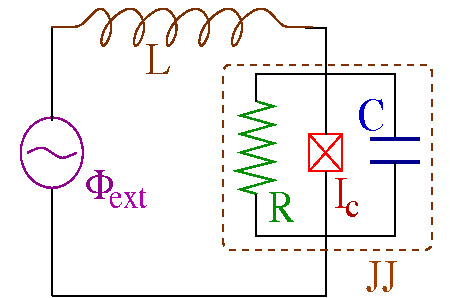
Figure 1: Equivalent electrical circuit model for a single SQUID that relies on the resistively and capacitively shunted junction (RCSJ) model of the Josephson junction (inside the dashed brown curve).

Consider three identical SQUIDS in an “axial geometry”, i.e., a SQUID trimer, sush that their axes lie on the same line as in Fig. 2. An externally applied magnetic field, whose direction is perpendicular to the rings of the SQUIDs (or equivalently is parallel to the SQUIDs’ axes) so that magnetic flux $\Phi_{ext}$ threads their loop, induces currents in the SQUID rings through Faraday’s law. These currents in turn produce their own magnetic field in each SQUID, whose magnetic flux threads the loops of the others. Thus, the SQUIDs are coupled together with magnetic dipole-dipole forces whose strength is quantified by their mutual inductance.

In order to derive the dynamical equations for the fluxes $\Phi_{n}$ ($n=1,2,3$) threading the loops of the SQUIDs, we first write their flux balance relations

$$\Phi_{1}=\Phi_{ext}+L\,I_{1}+M\,I_{2}+\frac{M}{8}\,I_{3},$$

$$\Phi_{2}=\Phi_{ext}+M\,I_{1}+L\,I_{2}+M\,I_{3},$$ (1)

$$\Phi_{3}=\Phi_{ext}+\frac{M}{8}\,I_{1}+M\,I_{2}+L\,I_{3},$$

where $\Phi_{n}$ and $I_{n}$ is the flux threading the loop of the $n-$th SQUID and the current flowing in the $n-$th SQUID, respectively, $L$ is the self-inductance of the SQUID ring (same for all three SQUIDs), and $M$ the mutual inductance between nearest-neighboring SQUIDs (i.e., between SQUIDs $1$ and $2$ and SQUIDs $2$ and $3$). Assuming that the strength of the dipole-dipole interaction between SQUIDs falls off as the inverse cube of their distance, we have adopted the value of $M/8$ for the coupling strength between SQUIDs $1$ and $3$.

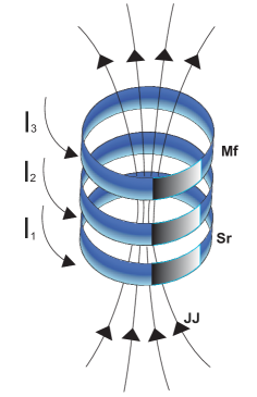
Figure 2: Schematic diagram of a SQUID trimer in the “axial geometry” subject to a magnetic field Mf, which are coupled together through their mutual inductance with strength $\lambda$. Sr is the superconducting ring, JJ is the Josephson Junction, and $I_{1}$, $I_{2}$, and $I_{3}$ are the induced currents.

By dividing Eqs. (1) with the self-inductance $L$, by rearranging terms, and by defining the dimensionless coupling strength as

$$\lambda=\frac{M}{L},$$ (2)

Eqs. (1) can be written in matrix form as

$${\bf\hat{\Lambda}}\vec{I}=\vec{\cal F},$$ (3)

where

$${\bf\hat{\Lambda}}=\begin{bmatrix}1&\lambda&\frac{\lambda}{8}\\[8.61108pt] \lambda&1&\lambda\\[8.61108pt] \frac{\lambda}{8}&\lambda&1\end{bmatrix},~{}~{}\vec{I}=\begin{bmatrix}I_{1}\\[8.61108pt] I_{2}\\[8.61108pt] I_{3}\end{bmatrix},~{}~{}\vec{\cal F}=\frac{1}{L}\begin{bmatrix}\Phi_{1}-\Phi_{ext}\\[8.61108pt] \Phi_{2}-\Phi_{ext}\\[8.61108pt] \Phi_{3}-\Phi_{ext}\end{bmatrix}.$$ (4)

The current flowing in the $n-$th SQUID is provided in terms of the flux $\Phi_{n}$ ($n=1,2,3$) threading its loop by the resistively and capacitively junction (RCSJ) model, as Likharev1986

$$I_{n}=-C\,\frac{d^{2}\Phi_{n}}{dt^{2}}-\frac{1}{R}\,\frac{d\Phi_{n}}{dt}-I_{c}\,\sin\left(2\pi\frac{\Phi_{n}}{\Phi_{0}}\right),$$ (5)

where $\Phi_{0}$ is the flux quantum and $t$ is the temporal variable. By multiplying Eq. (3) with the inverse of the matrix ${\bf\hat{\Lambda}}$, and by substituting the components of $\vec{I}$ using Eq. (5), we get

$$L\begin{bmatrix}C\frac{d^{2}\Phi_{1}}{dt^{2}}+\frac{1}{R}\frac{d\Phi_{1}}{dt}+\frac{2\pi}{\Phi_{0}}I_{c}\,\sin\left(2\pi\frac{\Phi_{1}}{\Phi_{0}}\right)\\[8.61108pt] C\frac{d^{2}\Phi_{2}}{dt^{2}}+\frac{1}{R}\frac{d\Phi_{2}}{dt}+\frac{2\pi}{\Phi_{0}}I_{c}\,\sin\left(2\pi\frac{\Phi_{2}}{\Phi_{0}}\right)\\[8.61108pt] C\frac{d^{2}\Phi_{3}}{dt^{2}}+\frac{1}{R}\frac{d\Phi_{3}}{dt}+\frac{2\pi}{\Phi_{0}}I_{c}\,\sin\left(2\pi\frac{\Phi_{3}}{\Phi_{0}}\right)\end{bmatrix}=\frac{1}{D}\begin{bmatrix}1-\lambda^{2}&-\lambda+\frac{\lambda^{2}}{8}&\lambda^{2}-\frac{\lambda}{8}\\[8.61108pt] -\lambda+\frac{\lambda^{2}}{8}&1-\frac{\lambda^{2}}{64}&-\lambda+\frac{\lambda^{2}}{8}\\[8.61108pt] \lambda^{2}-\frac{\lambda}{8}&-\lambda+\frac{\lambda^{2}}{8}&1-\lambda^{2}\end{bmatrix}\begin{bmatrix}\Phi_{1}-\Phi_{ext}\\[8.61108pt] \Phi_{2}-\Phi_{ext}\\[8.61108pt] \Phi_{3}-\Phi_{ext}\end{bmatrix}$$ (6)

, where

$$D\equiv\det\left({\bf\hat{\Lambda}}\right)=1-\frac{129}{64}\lambda^{2}+\frac{1}{4}\lambda^{3}.$$ (7)

In the following, the external flux is considered to be of the form

$$\Phi_{ext}=\Phi_{dc}+\Phi_{ac}\,\cos(\omega t),$$ (8)

i.e., it contains both a constant (dc) flux bias $\Phi_{dc}$ and an alternating (ac) flux of amplitude $\Phi_{ac}$ and frequency $\omega$.

Equations (7) and (8) are normalized using the relations

$$\phi_{n}=\frac{\Phi_{n}}{\Phi_{0}},~{}~{}~{}\phi_{ac,dc}=\frac{\Phi_{ac,dc}}{\Phi_{0}},~{}~{}~{}\tau=\frac{t}{\omega_{LC}^{-1}},~{}~{}~{}\Omega=\frac{\omega}{\omega_{LC}},$$ (9)

where $\omega_{LC}=1/\sqrt{LC}$ is the inductive-capacitive ($L\,C$) SQUID frequency. Eventually, the normalized equations read

$$\begin{bmatrix}\ddot{\phi}_{1}+\gamma\dot{\phi}_{1}+\beta\sin(2\pi\phi_{1})\\[8.61108pt] \ddot{\phi}_{2}+\gamma\dot{\phi}_{2}+\beta\sin(2\pi\phi_{2})\\[8.61108pt] \ddot{\phi}_{3}+\gamma\dot{\phi}_{3}+\beta\sin(2\pi\phi_{3})\end{bmatrix}=\frac{1}{D}\begin{bmatrix}1-\lambda^{2}&-\lambda+\frac{\lambda^{2}}{8}&\lambda^{2}-\frac{\lambda}{8}\\[8.61108pt] -\lambda+\frac{\lambda^{2}}{8}&1-\frac{\lambda^{2}}{64}&-\lambda+\frac{\lambda^{2}}{8}\\[8.61108pt] \lambda^{2}-\frac{\lambda}{8}&-\lambda+\frac{\lambda^{2}}{8}&1-\lambda^{2}\end{bmatrix}\begin{bmatrix}\phi_{1}-\phi_{ext}\\[8.61108pt] \phi_{2}-\phi_{ext}\\[8.61108pt] \phi_{1}-\phi_{ext}\end{bmatrix}$$ (10)

, and

$$\phi_{ext}(\tau)=\phi_{dc}+\phi_{ac}\cos(\Omega\tau),$$ (11)

where

$$\beta=\frac{I_{c}L}{\Phi_{0}},\qquad\gamma=\frac{1}{R}\sqrt{\frac{L}{C}}$$ (12)

is the rescaled SQUID parameter and the loss coefficient, respectively.

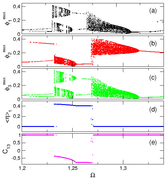
Figure 3: Bifurcation diagrams of (a) $\phi_{1}$ (black), (b) $\phi_{2}$ (red), and (c) $\phi_{3}$ (green), as a function of the driving frequency $\Omega$. (d) and (e) are the averaged in time Euclidean distance ${\langle\eta\rangle}_{\tau}$ and the correlation function $C_{13}$, respectively. Parameters: $\lambda=0.08$, $\phi_{ac}=0.02$, $\gamma=0.024$, $\phi_{dc}=0$, and $\beta=0.1369$.

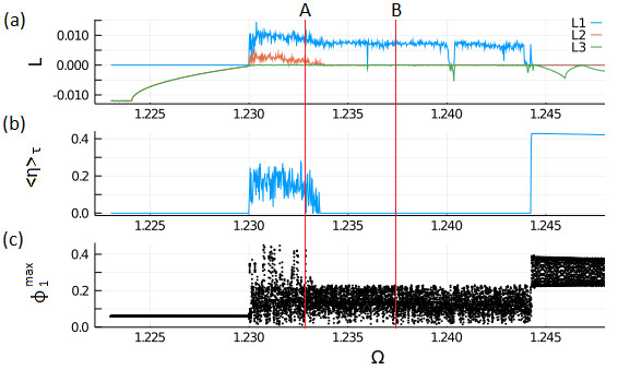
Figure 4: (a) The three largest Lyapunov exponents (the rest are negative), (b) the average of $\eta$ over time, $\left\langle\eta\right\rangle_{\tau}$, and (c) the maximum value of the magnetic flux $\phi_{1}$ in each driving cycle, $\phi_{1}^{max}$, as a function of the driving frequency $\Omega$. Red line A corresponds to $\Omega=1.233$ and B to $\Omega=1.2375$. We observe two main regions: The first one is between $\Omega=1.23$ and $\Omega=1.234$ and corresponds to intermittent hyperchaos synchronization ($0.38>\langle\eta\rangle_{\tau}>0.01$, $L_{1}>L_{2}>0,L_{3}=0$) while the second one lies between $\Omega=1.234$ and $\Omega=1.244$ and corresponds to complete chaos synchronization ($\left\langle\eta\right\rangle_{t}<0.01$, $L_{1}>0,L_{2}=L_{3}=0$). Parameters: $\lambda=0.1075$, $\phi_{ac}=0.02$, $\gamma=0.024$, $\phi_{dc}=0$, and $\beta=0.1369$.

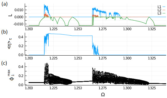
Figure 5: (a) The three largest Lyapunov exponents (the rest are negative), (b) the average of $\eta(\tau)$ over time, $\langle\eta\rangle_{\tau}$, and (c) the maximum value of the magnetic flux in SQUID $1$ in each driving cycle, $\phi_{1}^{max}$, as a function of the driving frequency $\Omega$. We observe three regions in which at least one Lyapunov exponent is positive: The first one lies between $\Omega=1.271$ and $\Omega=1.293$, in which the chaotic trajectories of SQUIDs $1$ and $3$ are completelly synchronized ($\langle\eta\rangle_{\tau}<0.01$ and $L_{1}>0$, $L_{2}=0$, $L_{3}=0$). Note however in this region the existence of at least two narrow windows in which the SQUID trimer exhibits periodic behavior along with synchronization of the trajectories between SQUIDs $1$ and $3$ ($\langle\eta\rangle_{\tau}<0.01$ and $L_{1}=0$, $L_{2},L_{3}<0$). The second and the third ones lie in the frequency range $(1.266,1.271)$ and $(1.216,1.22)$, respectively, in which the system exhibits hyperchaotic behavior ($L_{1}>L_{2}>0$, $L_{3}=0$). In the second region, intermittent chaos synchronization is observed between SQUIDs $1$ and $3$ ($0.01<\langle\eta\rangle_{\tau}<0.38$). In the third region however, the situation is more complicated since the value of $\langle\eta\rangle_{\tau}$ often exceeds the limiting value $0.38$ (see text). Parameters: $\lambda=0.1075$, $\phi_{ac}=0.025$, $\gamma=0.024$, $\phi_{dc}=0$, and $\beta=0.1369$.

In what follows, the external dc flux is set to zero, i.e., $\phi_{dc}=0$, for simplicity. The values of the SQUID model $\beta$ and $\gamma$ are obtained from Eqs. (12), using the experimentally determined parameters for the equivalent circuit elements $L=120~{}pH$, $C=1.1~{}pF$, $R=500~{}\Omega$, and $I_{c}=2.35~{}mA$ Zhang2015 . Using these values in Eqs. (12) we get $\beta=0.1369$ ($\beta_{L}\simeq 0.86$) and $\gamma=0.024$, while the $L\,C$ frequency is $f_{LC}=\omega_{LC}/2\pi=13.9~{}GHz$.

Note that most of the numerical work below has been performed with Julia programming language and the DynamicalSystems package Datseris2018 . The relevant codes used in this paper can be found in https://github.com/Joniald/Squid_Trimer.

III Chaos Synchronization and Quantitative Measures

As mentioned earlier, complete or intermittent chaos synchronization between the two SQUIDs at the ends of the trimer is observed, which we denote by $1$ and $3$. In order to quantify the synchronization between them, we adopt two different measures, namely, the instantaneous Euclidean distance:

$$\eta(\tau)=\sqrt{\left[\phi_{1}(\tau)-\phi_{3}(\tau)\right]^{2}+\left[\dot{\phi_{1}}(\tau)-\dot{\phi_{3}}(\tau)\right]^{2}},$$ (13)

in the reduced phase space of SQUIDs $1$ and $3$, which is an intuitive measure of the quality of synchronization Baker1998 , averaged over a time-interval $\Delta\tau$, $\langle\eta\rangle_{\tau}$, and the correlation coefficient between the normalized fluxes of SQUIDs $1$ and $3$:

$$C_{13}=\frac{\langle[\phi_{1}(\tau)-\mu_{1}][\phi_{3}(\tau)-\mu_{3}]\rangle}{\sigma_{1}\sigma_{3}},$$ (14)

where

$$\mu_{i}=\frac{1}{\Delta\tau}\int_{\tau_{tr}}^{\tau_{tr}+\Delta\tau}\phi_{i}(\tau)d\tau\rightarrow\frac{1}{M}\sum_{n=1}^{M}\phi_{i}(\tau_{n}),$$ (15)

is the temporal average of $\phi_{i}(\tau)$ ($i=1,3$) over the time interval $\Delta\tau$, $\tau_{tr}$ is the time allowed for transients to die out, $M$ is the number of integration time-steps in $\Delta\tau$, and $\sigma_{i}$ are the standard deviations of $\phi_{i}$, given by:

$$\sigma_{i}=\sqrt{\langle[\phi_{i}(\tau)-\mu_{i}]^{2}\rangle}.$$ (16)

Complete synchronization between the trajectories of SQUID $1$ and $3$ is achieved when $\langle\eta\rangle_{\tau}=0$, and $C_{13}=1$. For intermittent chaos synchronization, $1>\langle\eta\rangle_{\tau}>0$ and $C_{13}<1$. (The value of $C_{13}=-1$ if it ever occurs would indicate chaos anti-synchronization Kim2003 .)

The SQUID trimer exhibits chaotic dynamics in relatively wide parameter intervals. Here we choose a value for the amplitude of the alternating (ac) flux $\phi_{ac}=0.02$ which is relatively low and certainly within the experimentally accesible values of this quantity. In Figs. 3 (a)-(c), the bifurcation diagrams for the flux of all three SQUIDs are shown as functions of $\Omega$. Together we have plotted the averaged Euclidean distance $\langle\eta\rangle_{\tau}$ (Fig. 3 (d)) and the correlation function $C_{13}$ (Fig. 3 (e)). As it can be observed, the frequency interval in these figures is above the geometrical frequency $\Omega_{LC}=1$, and below the linearized SQUID frequency $\Omega_{SQ}=\sqrt{1+\beta_{L}}$ ($\simeq 1.36$ for the value of $\beta_{L}=0.86$ used in the simulations). The value of $\lambda=0.08$ used for obtaining the results are within the calculated ones in  Zhang2015 for this particular geometric configuration (e.g., the axial configuration). As it can be observed in all subfigures, there are several frequency intervals where the dynamics is chaotic in which SQUID $1$ and $3$ are completely synchronized ($\langle\eta\rangle_{\tau}=0$ and $C_{13}=1$. There are also intervals in which intermittent chaos synchronization appears. In the latter, $1>\langle\eta\rangle_{\tau}>0$ and $C_{13}<1$. Note that the two measures agree in all frequency intervals on whether SQUIDs $1$ and $3$ are completely or intermittently synchronized.

In order to identify precisely the frequency intervals in which the SQUID trimer exhibits chaotic dynamics, we calculate the full Lyapunov spectrum. A typical example is shown in Fig. 4 for $\phi_{ac}=0.02$ and $\lambda=0.1075$, where the three largest Lyapunov exponents $L_{1}>L_{2}>L_{3}$ (Fig. 4 (a)) are plotted together with $\langle\eta\rangle_{\tau}$ (Fig. 4 (b)), and the amplitude of the flux threading SQUID $1$, $\phi_{1}^{max}$ (Fig. 4 (c)). These results are obtained by initializing the SQUID trimer at $\Omega=1.233$ and performing a sweep in the decreasing direction in small steps $\Delta\Omega=2.5\times 10^{-5}$. For each value of $\Omega$, except for the first one, the solution obtained for the previous value of $\Omega$ is set as initial condition for the SQUID trimer.

The three largest Lyapunov exponents are sufficient for characterizing the dynamics of the SQUID trimer, while the remaining $L_{4}$, $L_{5}$, $L_{6}$, and $L_{7}$ are always negative. Note that since time $\tau$ is treated as a dependent variable (and this is why there are seven Lyapunov exponents instead of six), one of the exponents is always zero. As the driving frequency $\Omega$ decreases from the maximum shown value $\Omega=1.250$ down to $\Omega=1.244$, it is observed that the two largest Lyapunov exponents $L_{1}$ and $L_{2}$ are zero while the third largest is mostly negative ($L_{3}<0$), indicating quasiperiodic dynamics. There is no synchronization between SQUID $1$ and $3$ in this dynamical state as can be inferred by the corresponding values of $\langle\eta\rangle_{\tau}\simeq 0.42$. Note that at a particular frequency $\Omega=1.248$, the three largest Lyapunov exponents are all zero, i.e., $L_{1}=L_{2}=L_{3}=0$, indicating a bifurcation from one quasiperiodic dynamical state to another one.

At approximately $\Omega=1.244$, the SQUID trimer undergoes a quasiperiodicity to chaos transition and consequently the largest Lyapunov exponent $L_{1}$ becomes positive ($L_{1}>0$, blue curve) while $L_{3}$ becomes zero like $L2$ (green and orange curves). With further decreasing $\Omega$, the (positive) value of the largest exponent $L_{1}$ remains almost constant on average (note however the existence of a couple of narrow periodic windows where $L_{1}$ drops to zero) until $\Omega$ reaches $1.234$. Note that in this frequency interval, i.e., for $\Omega$ in $[1.244,1.234]$, in which the dynamics of the SQUID trimer is chaotic, SQUIDs $1$ and $3$ are completely synchronized as can be inferred from the corresponding values of $\langle\eta\rangle_{\tau}\simeq 0$ there.

At $\Omega=1.234$, the second largest Lyapunov exponent $L_{2}$ becomes also positive, while $L_{3}$ remains zero, indicating a chaos to hyperchaos transition. That value of $\Omega$ also signifies a transition from complete to intermittent chaos synchronization between SQUIDs $1$ and $3$. The hyperchaotic dynamical state persists down to $\Omega=1.230$. In the frequency interval $[1.230,1.234]$, as mentioned earlier, SQUID $1$ and $3$ exhibit intermittent chaos synchronization. This can be inferred from the value of $\langle\eta\rangle_{\tau}$ which is clearly above zero and strongly fluctuating but less than the limiting value of $0.38$. Indeed, we have empirically found that for $\langle\eta\rangle_{\tau}\leqslant 0.38$ we have intermittent chaos synchronization while for $\langle\eta\rangle_{t}>0.38$ the two SQUIDs, $1$ and $3$, are neither synchronized together nor with SQUID $2$ (middle SQUID). Finally, for even lower values of the driving frequency $\Omega$, i.e., for values in the interval $[1.223,1.230]$, a transition from a hyperchaotic to a periodic state occurs, and the maximum Lyapunov exponent becomes zero ($L_{1}=0,L_{2},L_{3}<0$).

Thus, in the results shown in Fig. 4, we can identify four different types of behavior that mostly dominate the dynamics:

(i) $\Omega$ in $(1.244,1.250]$: Quasiperiodicity ($L_{1}=L_{2}=0$, $L_{3}<0$) without any type of synchronization between SQUID $1$ and $3$ ($\langle\eta\rangle_{\tau}\simeq 0.42$).

(ii) $\Omega$ in $(1.234,1.244]$: Chaos ($L_{1}>0$, $L_{2}=L_{3}=0$), and complete chaos synchronization between SQUID $1$ and $3$ ($\langle\eta\rangle_{\tau}<0.01$). In practice, the values of $\langle\eta\rangle_{\tau}$ obtained in this dynamical state are all less than $0.01$.

Chaotic behavior in a system whose Lyapunov spectrum has one positive and two vanishing exponents, while all the others are negative, is referred to as “toroidal chaos” in a recent classification of chaotic regimes Letellier2021 .

(iii) $\Omega$ in $(1.230,1.234]$: Hyperchaos ($L_{1}>L_{2}>0$, $L_{3}=0$), and intermittent chaos synchronization between SQUID $1$ and $3$ ($0.38>\langle\eta\rangle_{\tau}>0.01$).

(iv) $\Omega$ in $[1.230,1.223]$: Periodic dynamics ($L_{1}=0$, $L_{2}<0$, $L_{3}<0$), with SQUIDs $1$ and $3$ being synchronized ($\langle\eta\rangle_{\tau}\simeq 0$).

By changing the parameters of the system we may observe a plethora of transitions between dynamical regions, as $\Omega$ is varied. To illustrate this, we have produced a similar plot to Fig. 4, for $\lambda=0.1075$ and $\phi_{ac}=0.025$. The results are shown in Fig. 5. Compared to Fig. 4, the scenario here presents additional dynamical regions, and a total of six different types of behavior which are the following:

(i) $\Omega$ in $(1.322,1.34]$: Periodic dynamics ($L_{1}=0$, $L_{2}<0$, $L_{3}<0$), with synchronization between SQUIDs $1$ and $3$ ($\langle\eta\rangle_{\tau}<0.01$).

(ii) $\Omega$ in $(1.293,1.322]$: Quasiperiodic dynamics ($L_{1}=L_{2}=0,L_{3}<0$), with synchronization between SQUIDs $1$ and $3$ ($\left\langle\eta\right\rangle_{\tau}<0.01$). In this interval, two bifurcations from a quasiperiodic state to another are visible for the values of $\Omega$ at which $L_{1}=L_{2}=L_{3}=0$.

(iii) $\Omega$ in $[1.271,1.293]$: Chaos ($L_{1}>0$, $L_{2}=L_{3}=0$), and complete chaos synchronization between SQUIDs $1$ and $3$ ($\left\langle\eta\right\rangle_{\tau}<0.01$). This is yet another case of toroidal chaos Letellier2021 already mentioned in the discussion of Fig. 4.

In this region of $\Omega$, there are also visible at least two windows in which the SQUID trimer exhibits periodic behavior with synchronized trajectories of SQUIDS $1$ and $3$. This dynamical behavior has been also observed in region (i) above, and it will not be further analyzed.

(iv) $\Omega$ in $(1.266,1.271]$: Hyperchaos ($L_{1}>L_{2}>0$, $L_{3}=0$), and intermittent chaos synchronization between SQUID $1$ and $3$ ($0.38>\left\langle\eta\right\rangle_{\tau}>0.01$).

(iv) $\Omega$ in $(1.244,1.266]$: Periodic dynamics ($L_{1}=0$, $L_{2}<0$, $L_{3}<0$), without synchronization between SQUIDs $1$ and $3$ ($\left\langle\eta\right\rangle_{\tau}>0.38$).

(v) $\Omega$ in $(1.22,1.244]$: Quasiperiodicity ($L_{1}=L_{2}=0$, $L_{3}<0$) without synchronization between SQUID $1$ and $3$ ($\left\langle\eta\right\rangle_{\tau}>0.38$). In this interval, three bifurcations from a quasiperiodic state to another are visible for the values of $\Omega$ at which $L_{1}=L_{2}=L_{3}=0$.

(vi) $\Omega$ in $(1.216,1.22]$: Hyperchaos ($L_{1}>L_{2}>0$, $L_{3}=0$). In this case, the quantity $\langle\eta\rangle_{\tau}$ fluctuates apparently randomly between values which either lie below or above the limiting one for intermittent chaos synchronization behavior, i.e., $\langle\eta\rangle_{\tau}=0.38$. By inspection of many of the corresponding solutions for the fluxes $\phi_{i}$ ($i=1,2,3$) in this frequency interval, we infer that for $\langle\eta\rangle_{\tau}<0.38$ the fluxes $\phi_{1}$ and $\phi_{3}$ are intermittently synchronized, while for $\left\langle\eta\right\rangle_{\tau}>0.38$ all the fluxes $\phi_{i}$ are unsynchronized.

(vii) $\Omega$ in $[1.2,1.216]$: Periodic dynamics ($L_{1}=0$, $L_{2}<0$, $L_{3}<0$), with synchronization between SQUIDs $1$ and $3$ ($\left\langle\eta\right\rangle_{\tau}<0.01$).

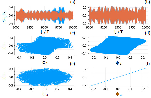
Figure 6: Chaos intermittent synchronization for the parameters of Fig. 4 and $\Omega=1.233$ (red line A). (a) Time series for $\phi_{1}$ and $\phi_{3}$. (c) Projection of the flow onto the $\phi_{1}-\phi_{2}$ plane. (e) Projection of the flow onto the $\phi_{1}-\phi_{3}$ plane. (b), (d), and (f) are the corresponding figures in the case of complete chaos synchronization for the parameters of Fig. 4 and $\Omega=1.2375$ (red line B).

We illustrate below a typical case of a hyperchaotic state (with accompanied intermittent chaos synchronization between SQUIDs $1$ and $3$) and a chaotic state (with complete chaos synchronization between SQUIDs $1$ and $3$). The corresponding values of $\Omega$ have been marked by the red horizontal lines A ($\Omega=1.233$) and B ($\Omega=1.2375$), respectively, in Fig. 4. The temporal evolution of the fluxes $\phi_{1}$ and $\phi_{3}$ in SQUIDs $1$ and $3$, respectively, have been plotted as a function of the normalized temporal variable $\tau$ divided by the driving period $T=\Omega/(2\pi)$ in Fig. 6(a) for $\Omega=1.233$ and Fig. 6(b) for $\Omega=1.2375$. Blue represents the flux in SQUID $1$, $\phi_{1}$, and red the flux in SQUID $3$, $\phi_{3}$. In Fig. 6(a), the temporal evolution of $\phi_{1}$ and $\phi_{3}$ is not synchronized although there are some windows in time where synchronization occurs. This is typical behavior of hyperchaos with chaos intermittent synchronization that will be discussed in more details in the next section. This behavior can be confirmed in both ($\phi_{1},\phi_{2}$) and ($\phi_{1},\phi_{3}$) plane projections of the trajectory as shown in Fig. 6(c) and (e). Complete chaos synchronized can be observed in Fig. 6(b) as the temporal evolution of $\phi_{1}$ and $\phi_{3}$ practically overlap. The projection of the flow onto the ($\phi_{1},\phi_{3}$) plane shown in Fig. 6(f) confirm this behavior. The projection of the flow onto the ($\phi_{1},\phi_{2}$) plane shown in Fig. 6(d) merely verifies that no synchronization occurs between SQUIDs $1$ and $2$.

IV The parameter space

As presented in the previous section, based on the time-averaged Euclidean distance $\langle\eta\rangle_{\tau}$, we can observe three main behaviors: Complete synchronization, intermittent synchronization and unsynchronized solutions. Moreover, by calculating the Lyapunov exponents we identify periodic solutions, quasiperiodicity, chaos and hyperchaos. In Fig. 7, a map of different dynamical regions based on the combined measurement of $\langle\eta\rangle_{\tau}$ and the maximum Lyapunov exponent are shown in ($\Omega,\lambda$) (Fig.7 (a)) and ($\Omega,\phi_{ac}$) (Fig.7 (b)) parameter space. We observe seven different areas. Periodic synchronization (PS) where $L_{1}=0,L_{2},L_{3}<0$ and $\langle\eta\rangle_{\tau}<0.01$, quasiperiodic synchronized solutions (QPS) where $L_{1}=L_{2}=0,L_{3}<0$ and $\langle\eta\rangle_{\tau}<0.01$, periodic unsynchronized solutions (PUn) where $L_{1}=0,L_{2},L_{3}<0$ and $0.38<\langle\eta\rangle_{\tau}$, quasiperiodic unsynchronized solutions (QPUn) where $L_{1}=L_{2}=0,L_{3}<0$ and $\left\langle\eta\right\rangle_{\tau}>0.38$, chaos synchronization (CS) where $L_{1}>0,L_{2}=L_{3}=0$ and $\left\langle\eta\right\rangle_{\tau}<0.01$, chaos intermittent synchronization (CI) where $L_{1}>0,L_{2}=L_{3}=0$ and $0.01<\left\langle\eta\right\rangle_{\tau}<0.38$, and finally hyperchaos intermittent synchronization (HCI) where $L_{1}>0,L_{2}>0,L_{3}=0$ and $0.01<\left\langle\eta\right\rangle_{\tau}<0.38$.

In both ($\Omega,\lambda$) and ($\Omega,\phi_{ac}$) parameter spaces, periodic synchronized (PS) and quasiperiodic synchronized (QPS) solutions occupy most of the plane. Next, the main dynamical behavior is concentrated in periodic unsynchronized (PUn) and quasiperiodic unsynchronized (QPUn) solutions. At the boundaries of these regions, we observe chaos synchronization (CS) and hyperchaos intermittent synchronization (HCI). It is remarkable that hyperchaos always appears with intermittent synchronization of $\phi_{1}(\tau)$ and $\phi_{3}(\tau)$. We have never observed synchronization or unsynchronized solutions between the trimer edges, in the presence of hyperchaos. The opposite is not true. Indeed, intermittent synchronization can also be observed in the chaotic regime (Fig. 7, blue color (CI)).

Four specific behaviors of non chaotic dynamics are shown in Fig. 8 for $\phi_{ac}=0.02$. The time series of the magnetic fluxes $\phi_{1}(\tau)$ and $\phi_{3}(\tau)$ (Fig. 8(a), left column), for $\Omega=1.22$ and $\lambda=0.16$, show a periodic synchronized solution between SQUID $1$ (red color) and SQUID $3$ (blue color). The corresponding time series of $\eta$ (Fig. 8(a), right column) which is close to zero also indicates a synchronization behavior. When $\Omega=1.24$ and $\lambda=0.07$, $\phi_{1}(\tau)$ and $\phi_{3}(\tau)$ oscillate out of phase, with different amplitudes, and $\eta$ also oscillates in time with an average value greater than $0.38$, an indication for a periodic unsynchronized solution (Fig. 8(b), left and right column). For ($\Omega=1.3,\lambda=0.14$) and ($\Omega=1.255$, $\lambda=0.1018$) the temporal evolution of the system is quasiperiodic. The magnetic fluxes of SQUIDs $1$ and $3$ oscillate in time with equal and different amplitudes in the left column of Figs. 8(c) and (d), respectively. In the case of synchronization the $\langle\eta\rangle_{\tau}$ quantifier between the trimer edges, i.e., between SQUIDs $1$ and $3$, is less than $0.01$ (Figs. 8(c), right column), while in the unsynchronized case $\eta$ has a periodic evolution with multiple frequencies due to the quasiperiodic behavior, and $0.38<\left\langle\eta\right\rangle_{\tau}$ (Fig. 8(d), right column).

Fig. 9 illustrates three other dynamical examples, this time in the chaotic regime. For $\Omega=1.235$ and $\lambda=0.1$ the temporal evolution of the system is chaotic and the output magnetic fluxes in SQUIDs $1$ and $3$ are identical, as shown in Fig. 9 (a), left column. This chaotic synchronization is confirmed by the evolution of $\eta$ close to zero in the right column. When $\Omega=1.23$ and $\lambda=0.125$ the time series of the trimer edges are chaotic but not identical. The three largest Lyapunov exponents associated with this evolution are ($0.007,0,0$). Nevertheless, there are some windows in time where synchronization occurs (Fig. 9(b), left column). This is a chaos intermittent synchronization where $\eta$ evolves, at some temporal intervals close to zero (synchronous behavior) while at others with large fluctuations between zero and one (Fig. 9(b), right column). The same dynamical behavior as in Fig. 9(b) is demonstrated in Fig. 9(c) for both $\phi_{1}(\tau)$ and $\phi_{3}(\tau)$ (left column) and $\eta$ quantifier (right column) where $\Omega=1.23$ and $\lambda=0.11$. However, in this case, the associated three largest Lyapunov exponents are ($0.015,0.002,0$). The system is now hyperchaotic, with more than one positive Lyapunov exponent and thus the behavior of the system is characterized as hyperchaotic intermittent synchronization.

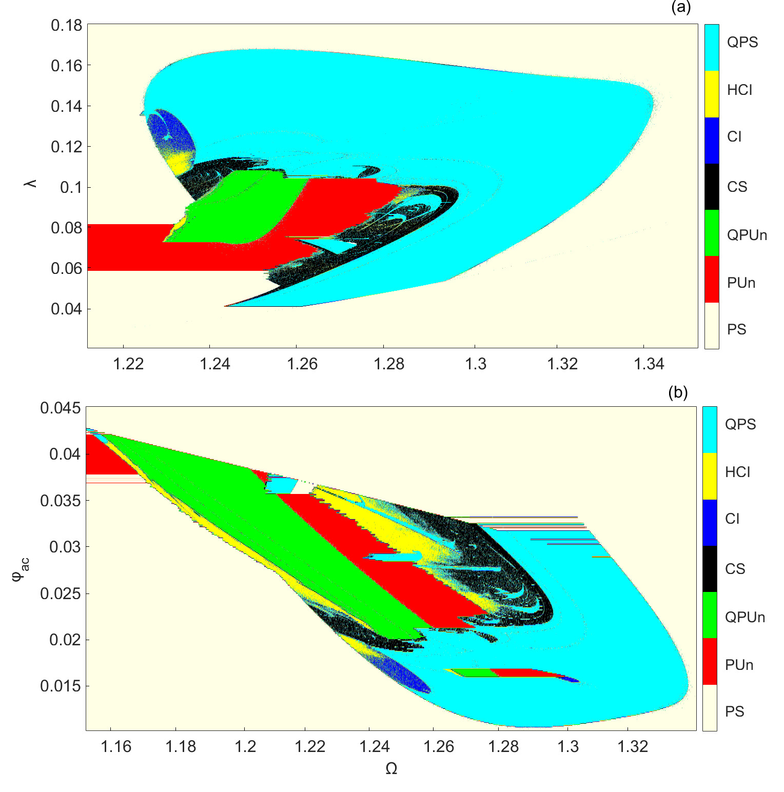
Figure 7: Map of different dynamical regions in the (a) ($\lambda,\Omega$) parameter space for $\phi_{ac}=0.02$, and (b) ($\Omega,\phi_{ac}$) parameter space for $\lambda=0.1075$. Depending on the three largest Lyapunov exponents ($L_{1}>L_{2}>L_{3}$) and $\left\langle\eta\right\rangle_{\tau}$ measurement, we observe seven different areas: Periodic synchronized solution (PS) where $L_{1}=0,L_{2},L_{3}<0$ and $\left\langle\eta\right\rangle_{\tau}<0.01$, Quasiperiodic synchronized (QPS) solutions where $L_{1}=L_{2}=0,L_{3}<0$ and $\left\langle\eta\right\rangle_{\tau}<0.01$, Periodic unsynchronized solution (PUn) where $L_{1}=0,L_{2},L_{3}<0$ and $0.38<\left\langle\eta\right\rangle_{\tau}$, Quasiperiodic unsynchronized solution (QPUn) where $L_{1}=L_{2}=0,L_{3}<0$ and $\left\langle\eta\right\rangle_{\tau}>0.38$, Chaos synchronization (CS) where $L_{1}>0,L_{2}=L_{3}=0$ and $\left\langle\eta\right\rangle_{t}<0.01$, Chaos intermittent synchronization (CI) where $L_{1}>0,L_{2}=L_{3}=0$ and $0.01<\left\langle\eta\right\rangle_{\tau}<0.38$ and finally Hyperchaos intermittent synchronization (HCI) where $L_{1}>0,L_{2}>0,L_{3}=0$ and $0.01<\left\langle\eta\right\rangle_{\tau}<0.38$.

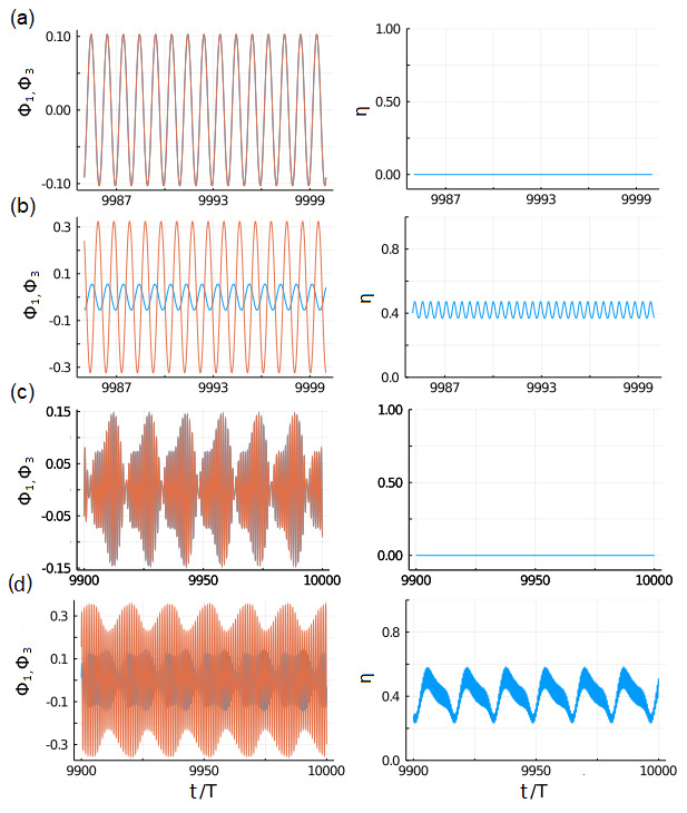
Figure 8: (a) Periodic synchronized solution (PS) for $\Omega=1.22$ and $\lambda=0.16$. (b) Periodic unsynchronized (PUn) solution for $\Omega=1.24$ and $\lambda=0.07$. (c) Quasiperiodic synchronized (QPS) solution for $\Omega=1.3$ and $\lambda=0.14$. (d) Quasiperiodic unsynchronized (QPUn) solution for $\Omega=1.255$ and $\lambda=0.1018$. In the left column, the fluxes $\phi_{1}$ and $\phi_{3}$ through the loops of SQUID $1$ (red line) and $3$ (blue line), respectively, are plotted as a function of $\tau/T$, where $T=\Omega/(2\pi)$. In the right column, the corresponding $\eta$ is plotted as a function of $\tau/T$. Other parameters: $\phi_{ac}=0.02$, $\gamma=0.024$, $\phi_{dc}=0$, and $\beta=0.1369$.

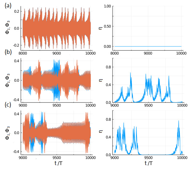
Figure 9: The fluxes $\phi_{1}$ and $\phi_{3}$ through the loops of SQUID $1$ (red line) and $3$ (blue line), respectively, are plotted as a function of $\tau/T$ in the left column, while the corresponding $\eta$s are plotted in the right column. (a) Chaos synchronization (CS) for $\Omega=1.235$ and $\lambda=0.1$. (b) Chaos intermittent synchronization (CI) for $\Omega=1.23$ and $\lambda=0.125$. (c) Hyperchaos intermittent synchronization (HCI) for $\Omega=1.23$ and $\lambda=0.11$. Other parameters: $\phi_{ac}=0.02$, $\gamma=0.024$, $\phi_{dc}=0$, and $\beta=0.1369$.

V Conclusions

To summarize, a trimer comprising three identical, magnetically coupled SQUIDs is investigated numerically with respect to chaotic synchronization phenomena. The SQUID trimer is a superconducting oligomer which serves as a highly complex system exhibiting a plethora of nonlinear dynamical effects. In this work, we focus on the synchronization between the two SQUIDs at the edges of the trimer informed by the corresponding dynamics of the system as a whole. By using suitable synchronization measures, like the correlation function and the Eulidean distance, we identify the types of synchronization in the relevant parameter spaces. Apart from complete chaotic synchronization between SQUIDs $1$ and $3$, we find that the SQUID trimer displays also intermittent chaotic synchronization between SQUIDs $1$ and $3$ where intervals of synchronization are interrupted by desynchronized activity. Calculations of the full Lyapunov exponent spectrum of the system reveal that the way from complete to intermittent synchronization is associated to chaos-hyperchaos transitions. In the intermittent synchonization case, we observe that the occurrence and the size of the intervals of the synchronized/desynchronized chaotic dynamics appear to be chaotic themselves. This requires further investigation and will be the subject of a future study.

VI ACKNOWLEDGEMENTS

This work was supported by the Ministry of Education and Science of the Russian Federation in the framework of the Increase Competitiveness Program of NUST “MISiS” (Grant number K4-2018-049). JH and NL acknowledge support by the General Secretariat for Research and Technology (GSRT) and the Hellenic Foundation for Research and Innovation (HFRI) (Code No. 203).

VII DATA AVAILABILITY

The data that support the findings of this study are available from the corresponding author upon reasonable request.

References

- (1) L. M. Pecora, T. L. Carroll, G. A. Johnson, D. J. Mar, and J. F. Heagy. Fundamentals of synchronization in chaotic systems, concepts, and applications. Chaos, 7, 1997.
- (2) R. Fermat and G. Solís-Perales. On the chaos synchronization phenomena. Phys. Lett. A, 262 (1):50–60, 1999.
- (3) A. Pikovsky, M. Rosenblum, and J. Kurths. Synchronization: A Universal Concept in Nonlinear Sciences. Cambridge University Press, Cambridge, 2003.
- (4) V. S. Anishchenko, T. E. Vadivasova, and G. I. Strelkova. Deterministic Nonlinear Systems. Springer International Publishing, Switzerland, 2014.
- (5) L. M. Pecora and T. L. Carroll. Synchronization in chaotic systems. Phys. Rev. Lett., 64 (8):821–824, 1990.
- (6) H. Fujisaka and T. Yamada. Stability theory of synchronized motion in coupled-oscillator systems. Prog. Theor. Phys., 69 (1):32–47, 1983.
- (7) V. S. Afraimovich, N. N. Verichev, and M. I. Ravinovich. Stochastic synchronization of oscillations in dissipative systems. Radiophys. Quantum Electron., 29 (9):795–803, 1986.
- (8) L. O. Chua, L. Kocarev, K. Eckert, and M. Itoh. Experimental chaos synchronization in chua’s circuit. Int. J. Bifurcation Chaos, 02:705–708, 1992.
- (9) V. S. Anishchenko, T. E. Vadivasova, D. E. Postnov, and M. A. Safonova. Synchronization of chaos. Int. J. Bifurcation Chaos, 2 (3):633–644, 1992.
- (10) L. O. Chua, M. Itoh, L. Kocarev, and K. Eckert. Chaos synchronization in chua’s circuit. J. Circuits Syst. Comput., 3 (1):93–108, 1993.
- (11) N. F. Rulkov. Images of synchronized chaos: Experiments with circuits. Chaos, 6 (3):262–278, 1996.
- (12) N. F. Rulkov and M.M. Sushchik. Robustness of synchronized chaotic oscillations. Int. J. Bifurcation Chaos, 7 (3):625–643, 1997.
- (13) E. Bilotta, F. Chiaravalloti, and P. Pantano. Synchronization and waves in a ring of diffusively coupled memristor-based chua’s circuits. Acta Appl. Math., 132:83–94, 2014.
- (14) Lj. Kocarec, K. S. Halle, K. Eckert, L. O. Chua, and U. Parlitz. Experimental demonstration of secure communications via chaotic synchronization. Int. J. Bifurcation Chaos, 2 (3):709–713, 1992.
- (15) L. Kocarev and U. Parlitz. General approach for chaotic synchronization with applications to communication. Phys. Rev. Lett., 74 (25):5028–5031, 1995.
- (16) J. Hizanidis, S. Deligiannidis, A. Bogris, and D. Syvridis. Enhancement of chaos encryption potential by combining all-optical and electrooptical chaos generators. IEEE J. Quantum Electron., 46 (11):1642–1649, 2010.
- (17) E. Mosekilde, Yu. Maistrenko, and D. Postnov. Chaotic Synchronization: Applications to Living Systems. World Scientific, Singapore, 2002.
- (18) T. Nowotny, R. Huerta, and M. I. Rabinovich. Neuronal synchrony: peculiarity and generality. Chaos, 18:037119, 2008.
- (19) H. G. Winful and L. Rahman. Synchronized chaos and spatiotemporal chaos in arrays of coupled lasers. Phys. Rev. Lett., 65 (13):1575–1578, 1990.
- (20) J. R. Terry, Jr. K. S. Thornburg, D. J. DeShazer, G. D. VanWiggeren, Shiqun Zhu, P. Ashwin, and Rajarshi Roy. Synchronization of chaos in an array of three lasers. Phys. Rev. E, 59 (4):4036–4043, 1999.
- (21) J. Shena, Y. Kominis, A. Bountis, and V. Kovanis. Spatial control of localized oscillations in arrays of coupled laser dimers. Phys. Rev. E, 102:012201, 2020.
- (22) Jinhu Lu, Tianshou Zhou, and Suochun Zhang. Chaos synchronization between linearly coupled chaotic systems. Chaos Soliton Fractals, 14:529–541, 2002.
- (23) E. Sánchez, D. Pazó, and M. A. Matías. Experimental study of the transitions between synchronous chaos and a periodic rotating wave. Chaos, 16:033122, 2006.
- (24) E. Tafo Wembe and R. Yamapi. Chaos synchronization of resistively coupled duffing systems: Numerical and experimental investigations. Commun. Nonlinear Sci. Numer. Simul., 14:1439–1453, 2009.
- (25) Junzhong Yang, Gang Hu, and Jinghua Xiao. Chaos synchronization in coupled chaotic oscillators with multiple positive lyapunov exponents. Phys. Rev. Lett., 80 (3):496–499, 1998.
- (26) S. K. Dana, B. Blasius, and J. Kurths. Experimental evidence of anomalous phase synchronization in two diffusively coupled chua oscillators. Chaos, 16:023111, 2006.
- (27) A. E. Hramov and A. A. Koronovskii. An approach to chaotic synchronization. Chaos, 14:603–610, 2004.
- (28) V. S. Anishchenko, A. N. Silchenko, and I. A. Khovanov. Synchronization of switching processes in coupled lorenz systems. Phys. Rev. E, 57 (1):316–322, 1998.
- (29) V. V. Astakhov, V. S. Anishchenko, T. Kapitaniak, and A. V. Shabunin. Synchronization of chaotic oscillators by periodic parametric perturbations. Physica D, 109:11–16, 1997.
- (30) V. Astakhov, A. Shabunin, T. Kapitaniak, and V. Anishchenko. Loss of chaos synchronization through the sequence of bifurcations of saddle periodic orbits. Phys. Rev. Lett, 79 (6):1014–1017, 1997.
- (31) V. Astakhov, M. Hasler, T. Kapitaniak, A. Shabunin, and V. Anishchenko. Effect of parameter mismatch on the mechanism of chaos synchronization loss in coupled systems. Phys. Rev. E, 58 (5):5620–5628, 1998.
- (32) S. V. Astakhov, A. Dvorak, and V. S. Anishchenko. Influence of chaotic synchronization on mixing in the phase space of interacting systems. Chaos, 23:013103, 2013.
- (33) Y. I. Boev, T. E. Vadivasova, and V. S. Anishchenko. Poincare recurrence statistics as an indicator of chaos synchronization. Chaos, 24:023110, 2014.
- (34) J. F. Heagy, T. L. Carroll, and L. M. Pecora. Desynchronization by periodic orbits. Phys. Rev. E, 52 (2):R1253–R1256, 1995.
- (35) A. Cenys, A. Namajunas, A. Tamasevicius, and T. Schneider. On-off intermittency in chaotic synchronization experiment. Phys. Lett. A, 213:259–264, 1996.
- (36) Jyh-Long Chern, Tzu-Chien Hsiao, Jiann-Shing Lih, Li-E Li, and Kenju Otsuka. Synchronized chaos and intermittent synchronization. Chin. J. Phys., 36 (5):667–676, 1996.
- (37) D. J. Gauthier and J. C. Bienfang. Intermittent loss of synchronization in coupled chaotic oscillators: Toward a new criterion for high-quality synchronization. Phys. Rev. Lett., 77 (9):1751–1754, 1996.
- (38) G. L. Baker, J. A. Blackburn, and H. J. T. Smith. Intermittent synchronization in a pair of coupled chaotic pendula. Phys. Rev. Lett., 81 (3):554–557, 1998.
- (39) J. A. Blackburn, G. L. Baker, and H. J. T. Smith. Intermittent synchronization of resistively coupled chaotic josephson junctions. Phys. Rev. B, 62 (9):5931–5935, 2000.
- (40) Sunghwan Rim, Myung-Woon Kim, Dong-Uk Hwang, Young-Jai Park, and Chil-Min Kim. Reconsideration of intermittent synchronization in coupled chaotic pendula. Phys. Rev. E, 64:060101(R), 2001.
- (41) Liang Zhao, Ying-Cheng Lai, and Chih-Wen Shih. Transition to intermittent chaotic synchronization. Phys. Rev. E, 72:036212, 2005.
- (42) Kenichiro Cho and Takaya Miyano. Intermittent and partial synchrony of coupled augmented rössler oscillators. Nonlinear Theory and Its Applications, IEICE, 9 (1):36–48, 2018.
- (43) S. M. Shariff. Multi-order intermittent chaotic synchronization of closed phase locked loop. International Journal of Modern Nonlinear Theory and Application, 7:48–55, 2018.
- (44) I. M. Kyprianidis, Ch. K. Volos, S. G. Stavrinides, I. N. Stouboulos, and A. N. Anagnostopoulos. On–off intermittent synchronization between two bidirectionally coupled double scroll circuits. Commun. Nonlinear. Sci. Numer. Simulat., 15:2192–2200, 2010.
- (45) T. Kapitaniak, K.-E. Thylwe, I. Cohen, and J. Wojewoda. Chaos-hyperchaos transition. Chaos Solitons Fractals, 5 (10):2003–2011, 1995.
- (46) T. Kapitaniak. Chaos synchronization and hyperchaos. J. Phys.: Conf. Ser., 23:317–324, 2005.
- (47) J. Hizanidis, N. Lazarides, and G. P. Tsironis. Flux bias-controlled chaos and extreme multistability in squid oscillators. Chaos, 28:063117, 2018.
- (48) J. Shena, N. Lazarides, and J. Hizanidis. Multi-branched resonances, chaos through quasiperiodicity, and asymmetric states in a superconducting dimer. Chaos, 30:123127, 2020.
- (49) M. Agaoglou, V. M. Rothos, and H. Susanto. Homoclinic chaos in a pair of parametrically-driven coupled squids. J. Phys.: Conf. Ser., 574:012027, 2015.
- (50) M. Agaoglou, V. M. Rothos, and H. Susanto. Homoclinic chaos in coupled squids. Chaos Solitons Fractals, 99:133–140, 2017.
- (51) N. Lazarides and G. P. Tsironis. Superconducting metamaterials. Phys. Rep., 752:1–67, 2018.
- (52) B. D. Josephson. Possible new effects in superconductive tunnelling. Phys. Lett. A, 1:251–253, 1962.
- (53) K. K. Likharev. Dynamics of Josephson Junctions and Circuits. Gordon and Breach, Philadelphia, 1986.
- (54) D. Zhang, M. Trepanier, O. Mukhanov, and S. M. Anlage. Tunable broadband transparency of macroscopic quantum superconducting metamaterials. Phys. Rev. X, 5:041045, 2015.
- (55) George Datseris. Dynamicalsystems.jl: A julia software library for chaos and nonlinear dynamics. Journal of Open Source Software, 3 23:598, 2018.
- (56) Chil-Min Kim, Sunghwan Rim, Won-Ho Kye, Jung-Wan Ryu, and Young-Jai Park. Anti-synchronization of chaotic oscillators. Phys. Lett. A, 320:39–46, 2003.
- (57) Christophe Letellier, Nataliya Stankevich, and Otto E. Rössler. Dynamical taxonomy: some taxonomic ranks to systematically classify every chaotic attractor. Submitted, 2021.