Radially symmetric scalar solitons

Abstract

A class of noncanonical effective potentials is introduced allowing stable, radially symmetric, solutions to first order Bogomol’nyi equations for a real scalar field in a fixed spacetime background. This class of effective potentials generalizes those found previously by Bazeia, Menezes, and Menezes [Phys.Rev.Lett. 91 (2003) 241601] for radially symmetric defects in a flat spacetime. Use is made of the “on-shell method” introduced by Atmaja and Ramadhan [Phys.Rev.D 90 (2014) 10, 105009] of reducing the second order equation of motion to a first order one, along with a constraint equation. This method and class of potentials admits radially symmetric, stable solutions for four dimensional static, radially symmetric spacetimes. Stability against radial fluctuations is established with a modified version of Derrick’s theorem, along with demonstrating that the radial stress vanishes. Several examples of scalar field configurations are given.

I Introduction

A class of noncanonical scalar field potentials of the form $U(r,\phi)=r^{-N}P(\phi)$, where $r$ is a radial variable, was introduced by Bazeia, Menezes, and Menezes Bazeia PRL03 for scalar field theories in $D$ space dimensions. It was shown that for certain constraints for $D$ and $N$ that radially stable scalar field configurations can exist, evading Derrick’s theorem Derrick . The $r^{-N}$ factor in $U(r,\phi)$ can emerge from a more fundamental theory which gives rise to an effective scalar field model. Potentials of this form have been physically motivated and considered in various contexts Bazeia PRD18 ,Bazeia PRR19 ,Andrade PRD19 ,Casana PRD20 ,Bazeia ppt20 . They give rise to field theoretic models with interesting properties, and are of mathematical interest, as well.

Attention has also been focused upon the possibility of evading Derrick’s theorem within the context of replacing a flat spacetime by curved spacetimes. (See, for example, Gonzalez RMF01 - Perivol PRD20 .) However, most of this work has been applied to systems with canonical scalar field potentials, which have no explicit dependence upon a radial variable, with an emphasis upon the effects of spacetime curvature on the stability of solitonic systems.

Presently, another class of potentials of the more general form $V(r,\phi)=F(r)P(\phi)$ is introduced in order to solve first order Bogomol’nyi equations for a scalar field $\phi(r)$ in a fixed static, radially symmetric four dimensional spacetime background. The nontopological solitonic solutions depend upon the assumed form of $P(\phi)$ and the form of the spacetime metric. These solutions are also found to minimize the energy and to be radially stable.  The radial stability can be established with a modified version of Derrick’s theorem Derrick , along with showing that the radial stress vanishes. The first order Bogomol’nyi equations can be solved using the “on-shell” type of method introduced by Atmaja and Ramadhan Atmaja PRD14 whereby a term is added and subtracted from the second order Euler-Lagrange equations of motion, thereby allowing a split of the second order differential equation (DE) into one first order Bogomol’nyi DE plus a constraint equation. (See also, Adam JHEP16 ,Atmaja JHEP16 .) The solution to these equations automatically satisfies the second order equation of motion. Here, this procedure is adapted to a single static, radially symmetric scalar field $\phi(r)$ for a particular type of potential $V(r,\phi)=F(r)P(\phi)$ whose function $F(r)$ depends upon the spacetime metric $g_{\mu\nu}$. Furthermore, this solution $\phi(r)$ provides a lower bound on the energy, and the scalar configuration described by $\phi(r)$ is shown to be stable against radial collapse or expansion.

The possibility of scalarization of gravitational sources, such as neutron stars, was introduced by Damour and Esposito-Farese Damour PRL93 in the context of scalar-tensor theory expressed in an Einstein frame. There, the response of a scalar field near a gravitational source was due to strong field effects associated with high curvature. Although a spontaneous scalarization can occur due to gravitational effects, the concept of scalarization can be extended to situations where other fields are involved. An example is provided by Maxwell-scalar theory, where a real valued scalar field couples nonminimally to the Maxwell field via a coupling function, say $\varepsilon(\phi)$, through an interaction term $-\frac{1}{4}\varepsilon(\phi)F_{\mu\nu}F^{\mu\nu}$. A scalar field may form around a compact object, even in a flat Minkowski spacetime (see, e,g, Bazeia ppt20 and Herdeiro PRD21 , and references therein). Models involving the formation of a scalar cloud around some source in a fixed spacetime background can serve as toy models of more realistic processes where back reactions upon the spacetime can be taken into account. Here, we examine the case of a scalar field responding to another, unspecified, field through an effective scalar potential $V(r,\phi)$. In particular, we consider the radially stable solutions of a first order Bogomol’nyi equation.

Examples of how an effective scalar potential can arise from interactions with other fields are provided in Section 2, and a BPS ansatz for obtaining Bogomol’nyi equations and solutions is presented in Section 3. The radial stability of the solutions is discussed in Section 4. Several examples of application are provided in Section 5. Section 6 concludes with a brief summary. Details regarding stability arguments are relegated to an appendix.

II An effective potential

A potential of the form $V(r,\phi)=F(r)P(\phi)=\frac{1}{f^{2}h}P(\phi)$ that is considered here can arise naturally as an effective scalar potential for a real scalar field $\phi$ that interacts with another field. Two such examples are provided here.

II.1 Interacting scalars

Consider a model of two interacting real scalar fields, $\phi$ and $\chi$, described by

$$\mathcal{L}=\frac{1}{2}\partial_{\mu}\phi\partial^{\mu}\phi+\frac{1}{2}K(\phi)\partial_{\mu}\chi\partial^{\mu}\chi$$ (1)

The equations of motion are given by

$$\nabla_{\mu}\nabla^{\mu}\phi-\frac{1}{2}(\partial_{\phi}K)(\partial_{\mu}\chi\partial^{\mu}\chi) =0$$ (2a)

$$\frac{1}{2}\nabla_{\mu}[K(\phi)\partial^{\mu}\chi] =0$$ (2b)

Assume now a radially symmetric (i.e., spherical or cylindrical symmetry) ansatz for time independent fields in a static, radially symmetric, four dimensional spacetime, $\phi=\phi(r)$ and $\chi=\chi(r)$. Also, denote $g=|\det g_{\mu\nu}|$ and let the radial part of $\sqrt{g}$ be designated by $f(r)$ and define $|g^{rr}|=h(r)$ where $r$ is the radial variable. In this case the equations of motion (2) reduce to

$$-\frac{1}{f}\partial_{r}(fh\partial_{r}\phi)+\frac{1}{2}(\partial_{\phi}K)[h(\partial_{r}\chi)^{2}] =0$$ (3a)

$$\partial_{r}[fhK(\phi)\partial_{r}\chi] =0$$ (3b)

From (3b) it follows that

$$\partial_{r}\chi=\frac{C}{fhK(\phi)}$$ (4)

where $C$ is a constant. From (4) we have

$$\frac{1}{2}K(\phi)\partial_{\mu}\chi\partial^{\mu}\chi=\frac{1}{2}K(\phi)(\partial_{r}\chi\partial^{r}\chi)=-\frac{1}{2}Kh(\partial_{r}\chi)^{2}=-\frac{1}{2f^{2}h}\frac{C^{2}}{K(\phi)}$$ (5)

Using (5), (1) yields an effective Lagrangian for the field $\phi$, $\mathcal{L}\rightarrow\frac{1}{2}\partial_{\mu}\phi\partial^{\mu}\phi-V(r,\phi)$, where the effective potential is

$$V(r,\phi)=-\frac{1}{2}K(\phi)\partial_{\mu}\chi\partial^{\mu}\chi=\frac{1}{2f^{2}h}\frac{C^{2}}{K(\phi)}=F(r)P(\phi)$$ (6)

where $F(r)=1/(f^{2}h)$ and $P(\phi)=\frac{1}{2}C^{2}K^{-1}(\phi)$. The equation of motion for $\phi$ can now be written as

$$\square\phi+\partial_{\phi}V(r,\phi)=0$$ (7)

II.2 Maxwell-scalar theory

A second example is provided by a Maxwell-scalar model involving a real, massless scalar field $\phi$ coupled nonminimally to an abelian Maxwell field $F_{\mu\nu}$. The Lagrangian is

$$\mathcal{L}=\frac{1}{2}\partial_{\mu}\phi\partial^{\mu}\phi-\frac{1}{4}\varepsilon(r,\phi)F_{\mu\nu}F^{\mu\nu}-J^{\nu}A_{\nu}$$ (8)

where $\varepsilon(r,\phi)$ is a nonminimal coupling function which may display a tachyonic instability that can depend upon the radial distance $r$ from the coordinate origin. We want to consider the spatial region exterior to the source of charge $Q$, i.e., the region of space where $J^{\nu}\rightarrow 0$. The equations of motion that follow from (8) are

$$\begin{array}[c]{cc}\nabla_{\mu}\nabla^{\mu}\phi+\frac{1}{4}(\partial_{\phi}\varepsilon)F_{\mu\nu}F^{\mu\nu}+\partial_{\phi}J^{\nu}A_{\nu}=0\vskip 3.0pt plus 1.0pt minus 1.0pt&\\ \nabla_{\mu}(\varepsilon F^{\mu\nu})=J^{\nu}&\end{array}$$ (9)

(A metric with signature $(+,-,-,-)$ is assumed. See Eq.(15) below.) Using $F_{\mu\nu}F^{\mu\nu}=-2(\mathbf{E}^{2}-\mathbf{B}^{2})$ and setting $J^{\nu}=0$ and $\mathbf{B}=0$, these reduce to

$$\begin{array}[c]{cc}\nabla_{\mu}\nabla^{\mu}\phi-\frac{1}{2}(\partial_{\phi}\varepsilon)\mathbf{E}^{2}=0\vskip 3.0pt plus 1.0pt minus 1.0pt&\\ \nabla_{\mu}(\varepsilon F^{\mu\nu})=0&\end{array}$$ (10)

Assuming radial symmetry, the Maxwell equation reduces to $\nabla_{r}(\varepsilon F^{r0})=\frac{1}{\sqrt{g}}\partial_{r}(\sqrt{g}\varepsilon F^{r0})=\frac{1}{f}\partial_{r}(f\varepsilon F^{r0})=0$ which is solved by

$$F^{r0}(r,\phi)=\frac{Q}{f(r)\varepsilon(r,\phi)},\ \ \ F_{r0}=g_{rr}g_{00}F^{r0}=-\frac{g_{00}Q}{f(r)h(r)\varepsilon(r,\phi)}$$ (11)

where $g_{rr}=1/g^{rr}$ and we define a “rationalized charge” $Q=Q_{0}/4\pi$, (or “rationalized linear charge density” $Q=Q_{0}/2\pi$) with $Q_{0}$ representing the actual charge/charge density, and

$$\mathbf{E}^{2}=-F_{r0}F^{r0}=\frac{g_{00}|g_{rr}|Q^{2}}{f^{2}\varepsilon^{2}}=\frac{g_{00}Q^{2}}{f^{2}h\varepsilon^{2}}$$ (12)

An effective Lagrangian for the scalar field $\phi$ is

$$\mathcal{L}=\frac{1}{2}\partial_{\mu}\phi\partial^{\mu}\phi+\frac{1}{2}\varepsilon(r,\phi)\mathbf{E}^{2}=\frac{1}{2}\partial_{\mu}\phi\partial^{\mu}\phi+\ \frac{g_{00}Q^{2}}{2f^{2}h}\varepsilon^{-1}\ (r,\phi)$$ (13)

Now define an effective potential

$$V(r,\phi)=\frac{1}{2}\varepsilon\mathbf{E}^{2}=\frac{g_{00}Q^{2}}{2f^{2}h}\varepsilon^{-1}(r,\phi)$$ (14)

An implementation of a BPS ansatz (presented below) will allow the coupling function to be expressed as $g_{00}Q^{2}\varepsilon^{-1}(r,\phi)=X^{2}(\phi)$. Using the expression (12) for $\mathbf{E}^{2}(r,\phi)\propto\varepsilon^{-2}(r,\phi)$, we see that for the ansatz solutions $\phi(r)$ we have, by (14), $V(r,\phi)=\frac{1}{2}\varepsilon\mathbf{E}^{2}\rightarrow\frac{1}{2f^{2}h}X^{2}$, and $-\frac{1}{2}(\partial_{\phi}\varepsilon)\mathbf{E}^{2}=+\partial_{\phi}(\frac{1}{2}\varepsilon\mathbf{E}^{2})$, so that an effective scalar potential appearing in the equation of motion for $\phi$ has the form $V(r,\phi)=\frac{1}{2}\varepsilon(r,\phi)\mathbf{E}^{2}(r,\phi)\rightarrow\frac{1}{2f^{2}h}X^{2}(\phi)$. In this case the scalar field equation of motion takes its standard form $\square\phi+\partial_{\phi}V(r,\phi)=0$.

To summarize, a scalar field $\phi$ can interact with other fields (e.g., scalars and gauge fields Atmaja PRD14 -Atmaja JHEP16 ) with an effective scalar potential of the form $V(r,\phi)=\frac{1}{f^{2}h}P(\phi)$. Scalar models with such an effective potential will be seen to have radially stable time independent solutions that obey a first order Bogomol’nyi equation.

III BPS ansatz

The spacetime geometries considered here are assumed to be fixed, i.e., back reactions of the scalar field upon the metric are ignored. The scalar field is assumed to be minimally coupled to the gravitational sector, that is, the action is written in an Einstein frame. We consider 4D metrics with radial symmetry (spherical or cylindrical) of the form

$$\left\{\begin{array}[c]{ll}ds^{2}=A(r)dt^{2}-B(r)dr^{2}-R^{2}(r)(d\theta^{2}+\sin^{2}\theta d\varphi^{2}),&\text{(spherical symmetry) }\vskip 6.0pt plus 2.0pt minus 2.0pt\\ ds^{2}=A(r)dt^{2}-B(r)dr^{2}-\rho^{2}(r)d\varphi^{2}-\zeta^{2}(r)dz^{2},&\text{(cylindrical symmetry)}\end{array}\right.$$ (15)

in which case we have $\sqrt{g}=\sqrt{AB}R^{2}\sin\theta$ for spherical symmetry and $\sqrt{g}=\sqrt{AB}\rho\zeta$ for cylindrical symmetry Trenda EJP , where $g=|\det g_{\mu\nu}|$. (The functions $A(r)$ and $B(r)$ for the cylindrical case are generally different from those for the spherical case.) We represent the radial part of $\sqrt{g}$ by

$$f(r)=\sqrt{A(r)B(r)C(r)}$$ (16)

where $\sqrt{C(r)}$ is given by

$$\sqrt{C(r)}=\left\{\begin{array}[c]{ll}R^{2}(r),&\text{(spherical symmetry)\vskip 6.0pt plus 2.0pt minus 2.0pt}\\ \rho(r)\zeta(r),&\text{(cylindrical symmetry)}\end{array}\right.$$ (17)

The Lagrangian for the real scalar field $\phi$ is given by

$$\mathcal{L}=\frac{1}{2}\partial^{\mu}\phi\partial_{\mu}\phi-V(r,\phi),\ \ \ V(r,\phi)=F(r)P(\phi)$$ (18)

where the noncanonical potential $V(r,\phi)=F(r)P(\phi)$ depends not only upon the scalar field $\phi$, but also has an explicit dependence upon the radial coordinate $r$, as in Ref Bazeia PRL03 . We consider static, radially symmetric solutions $\phi(r)$, for which the Lagrangian can be written as

$$\mathcal{L}=\frac{1}{2}g^{rr}(r)(\partial_{r}\phi)^{2}-F(r)P(\phi)$$ (19)

where $g^{rr}(r)=1/g_{rr}(r)=-1/B(r)$ and $\partial_{r}=\partial/\partial r$.

The equation of motion following from (18) is given by $\nabla_{\mu}\nabla^{\mu}\phi+\partial_{\phi}V(r,\phi)=0,$ or

$$\frac{1}{\sqrt{g}}\partial_{r}(\sqrt{g}g^{rr}\partial_{r}\phi)+\partial_{\phi}V=0$$ (20)

for $\phi=\phi(r)$, with $\partial_{\phi}V=\partial V/\partial\phi$. We can also define $h(r)\equiv|g^{rr}(r)|=1/B(r)$, or $g^{rr}=-h$ for our metric signature. The equation of motion (20) then reduces to

$$\partial_{r}[f(r)h(r)\partial_{r}\phi]=f(r)\partial_{\phi}V(r,\phi)$$ (21)

We now use the method of Atmaja and Ramadhan Atmaja PRD14 to generate a first order Bogomol’nyi equation by subtracting a term $\partial_{r}X(\phi)$ from both sides of (21):

$$\partial_{r}[f(r)h(r)\partial_{r}\phi-X(\phi)]=f(r)\partial_{\phi}V(r,\phi)-\partial_{r}X(\phi)$$ (22)

where the function $X=X(\phi)$ and $\partial_{r}X(\phi)=\partial_{\phi}X(\phi)\partial_{r}\phi$. The Euler-Lagrange equation of motion, i.e., equation (22) is then solved by solutions to the set of equations

$$f(r)h(r)\partial_{r}\phi=X(\phi),\ \ \ f(r)\partial_{\phi}V(r,\phi)=\partial_{\phi}X(\phi)\partial_{r}\phi$$ (23)

The first equation is the first order Bogomol’nyi equation, and the second equation gives the form of the potential $V$ in terms of $X(\phi)$ and $r$, since

$$\partial_{\phi}V=\partial_{\phi}X\cdot\frac{1}{f^{2}h}X=\frac{1}{2f^{2}h}\partial_{\phi}X^{2}$$ (24)

Integrating gives a potential $V=(2f^{2}h)^{-1}(X^{2}+c)$. Setting the constant $c=0$ and requiring that the function $X(\phi)$ is chosen so that $V$ is everywhere finite for a finite energy solution, then yields

$$V(r,\phi)=\frac{1}{2f^{2}(r)h(r)}X^{2}(\phi)$$ (25)

where $1/h=|g_{rr}|=B$. The second order equation of motion is then reduced to a first order one, along with a constraint on the form of $V(r,\phi)$:

$$\partial_{r}\phi(r)=\frac{1}{fh}X(\phi),\ \ \ \ \ V(r,\phi)=\frac{1}{2f^{2}h}X^{2}(\phi)=F(r)P(\phi)$$ (26)

We can identify $F(r)=(f^{2}h)^{-1}$ and $P(\phi)=\frac{1}{2}X^{2}(\phi)$. Upon choosing a suitable form for $X(\phi)$ that keeps the energy $E$ (or, energy per unit length for cylindrical symmetry) of the scalar field configuration finite, the Bogomol’nyi equation is solved by

$$\int\frac{d\phi}{X(\phi)} =\int\frac{dr}{f(r)h(r)},$$ (27a)

$$V(r,\phi) =\frac{1}{2f^{2}(r)h(r)}X^{2}(\phi)$$ (27b)

We note that for $h=1$ and $f=r^{N}$ this coincides with the form of the potential introduced in Ref. Bazeia PRL03 for flat spacetimes, with the identification $X(\phi)=W_{\phi}(\phi)=\partial_{\phi}W$, where $W(\phi)$ is a superpotential.

IV Energy and stability

The component of the stress-energy tensor associated with the energy density of the static scalar field $\phi(r)$ is $T_{0}^{0}=-\mathcal{L}=-[\frac{1}{2}g^{rr}(\partial_{r}\phi)^{2}-V]$, which we will also label as $\mathcal{H}$. From (15) we have $g^{rr}=-h(r)=-B^{-1}(r)$ so that $\mathcal{H}=\frac{1}{2}h(\partial_{r}\phi)^{2}+V$. From (26) we have gradient and potential contributions $\mathcal{H}_{g}=\frac{1}{2}h(\partial_{r}\phi)^{2}$ and $\mathcal{H}_{p}=V(r,\phi)=\frac{1}{2f^{2}h}X^{2}(\phi)=\frac{1}{f^{2}h}P(\phi)$. For the ansatz solutions (26) the gradient and potential parts are connected by $X(\phi)$ and contribute equally, but for an arbitrary solution to the second order equation of motion we consider the gradient and potential parts separately in applying an approach to analyze stability. Stability for the ansatz solutions is then demonstrated by connecting the gradient and potential pieces.

The energy of the scalar field is $E=\int T_{0}^{0}\sqrt{g}d^{3}x$, so that upon removing the integrations over the nonradial coordinates (see Appendix) we have an energy parameter $\mathcal{E}$, given by

$$\mathcal{E}=\int T_{0}^{0}f(r)dr=\int\mathcal{H}f(r)dr$$ (28)

For a stable solution $\phi(r)$ we require $\mathcal{E}$ to be finite, and to represent a stable minimum of the energy. In order to determine whether a static, radially dependent solution $\phi(r)$ represents a stable minimum of the action and energy, we follow the line of reasoning used in Derrick’s theorem Derrick . A solution $\phi(r)$ is allowed to be distorted by making the replacements $\phi(r)\rightarrow\phi_{\lambda}(r)=\phi(\lambda r)$ and $\mathcal{E}\rightarrow\mathcal{E}_{\lambda}$ where $\mathcal{E}_{\lambda}$ is the energy parameter $\mathcal{E}$ with $\phi$ replaced by $\phi_{\lambda}$. Upon allowing the parameter $\lambda$ to vary, we require that a solution representing a stable minimum satisfy $\delta\mathcal{E}=0$ and $\delta^{2}\mathcal{E}\geq 0$, or, in terms of $\mathcal{E}_{\lambda}$,

$$\text{(i)\ \ }\frac{d\mathcal{E}_{\lambda}}{d\lambda}\Big{|}_{\lambda=1}\ =0$$ (29a)

$$\text{(ii)\ }\frac{d^{2}\mathcal{E}_{\lambda}}{d\lambda^{2}}\Big{|}_{\lambda=1} \geq 0$$ (29b)

The energy $\mathcal{E}_{\lambda}$ can be written as a sum of two independent parts, $I_{1\lambda}$, representing the gradient contribution $\mathcal{H}_{g}=\frac{1}{2}h(\partial_{r}\phi)^{2}$ to the energy, and $I_{2\lambda}$, representing the contribution from the potential, $\mathcal{H}_{p}=V(r,\phi)$. It is shown (see Appendix) that for any radially symmetric ansatz solution satisfying (26) with finite energy (or finite energy per unit length) in a spacetime with a metric of the form given by (15), the stability of the solution, as required by (29), is guaranteed.

Additionally, it is seen that the radial stress vanishes, $T_{r}^{r}=0$, using the ansatz (26). Using $T_{r}^{r}=\partial^{r}\phi\partial_{r}\phi-g_{r}^{r}\mathcal{L}$, we find

$$T_{r}^{r}=-\frac{1}{2}h(\partial_{r}\phi)^{2}+V(r,\phi)=0$$ (30)

where (26) has been used. This indicates a stability against spontaneous radial collapse or expansion. We also note that the result $T_{rr}=0$ implies

$$\partial_{r}\phi=\pm\sqrt{2|g_{rr}|V}=\pm(fh)^{-1}X$$ (31)

(This is a radial generalization of the familiar one-dimensional linear result $\partial_{x}\phi(x)=\pm\sqrt{2V(\phi)}=\pm\partial_{\phi}W(\phi)$, where $W(\phi)$ is a superpotential, with $X$ playing the role of $\partial_{\phi}W$.) The nonzero stress components for the ansatz solutions are $T_{\xi}^{\xi}=-g_{\xi}^{\xi}\mathcal{L}=T_{0}^{0}=\mathcal{H}(r)$ (no sum on $\xi$), where $\xi$ represents a nonradial coordinate, with $T_{\xi}^{\xi}$ independent of $\xi$.

We note that for ansatz solutions satisfying (26) we have $\mathcal{H}_{g}=\mathcal{H}_{p}$ and therefore $\mathcal{H}=T_{0}^{0}=2V(r,\phi)=\frac{1}{f^{2}(r)h(r)}X^{2}(\phi)$.

V Examples

Several examples are now given for different metrics, where a form of $X(\phi)$ is chosen to yield $P(\phi)=\frac{1}{2}X^{2}(\phi)$ corresponding to the ubiquitous and interesting Higgs-type of potential. The spacetime background is taken to be fixed - no back reaction of the scalar on the background geometry is considered. It is assumed that the scalar stress-energy is negligible in comparison to that of the source, and the scalar field $\phi$ has no direct interaction with the source beyond a response to the background geometry.

(1) Spherical $\phi^{4}$ bubble: Consider a spherical scalar field configuration in a flat spacetime with metric given by

$$ds^{2}=dt^{2}-dr^{2}-r^{2}(d\theta^{2}+\sin^{2}\theta d\varphi^{2})$$ (32)

In this case $f(r)=r^{2}=\sqrt{g}/\sin\theta$ and $h=|g^{rr}|=1$. We choose

$$X(\phi)=\lambda(\eta^{2}-\phi^{2}),\ \ \ \ V(r,\phi)=\frac{1}{2f^{2}h}X^{2}(\phi)=\frac{\lambda^{2}}{2r^{4}}(\eta^{2}-\phi^{2})^{2}$$ (33)

where (25) has been used, and we take $\lambda$ and $\eta$ to be positive constants. With (27), $\int\frac{d\phi}{X(\phi)}=\int\frac{dr}{f(r)h(r)}$ gives

$$\int\frac{d\phi}{(\eta^{2}-\phi^{2})}=\lambda\int\frac{dr}{r^{2}}\implies-\frac{1}{\eta}\tanh^{-1}(\phi/\eta)=-\lambda(\frac{1}{r}+C)$$ (34)

Setting the integration constant $C=-1/R$ gives the solution

$$\phi(r)=\eta\tanh\Big{[}k\Big{(}\frac{1}{r}-\frac{1}{R}\Big{)}\Big{]},\ \ \ k=\lambda\eta\equiv r_{0}$$ (35)

With this solution we have $\phi(r)$ remaining everywhere finite. For $\phi(r)=+\eta\tanh[k(\frac{1}{r}-\frac{1}{R})]$ we have

$$\phi(r)\rightarrow\left\{\begin{array}[c]{ll}+\eta,&r\rightarrow 0\\ -\eta\tanh(\frac{k}{R}),&r\rightarrow\infty\end{array}\right\}$$ (36)

The solution $\phi/\eta$ is a monotonically decreasing function of $r$ with asymptotic value of $\phi\rightarrow-\eta\tanh(\frac{k}{R})$ (Fig1). For $\phi$ and $\eta$ having canonical mass dimension 1, we have a mass dimension of $-1$ for $k=\lambda\eta$, so that $\lambda$ has mass dimension $-2.$ We can write $\lambda\eta=k=r_{0}$ where $r_{0}$ is some radial constant. The configuration (35) suggests the existence of a bubble wall centered somewhere near $r\sim R$ where the energy density $\mathcal{H}(r)$ maximizes (Fig1). This is a static, radially stable solution to the equation of motion.

The energy density (28) of the solution (35) is

$$\mathcal{H}=\frac{1}{r^{4}}X^{2}(\phi)=\frac{\lambda^{2}}{r^{4}}(\eta^{2}-\phi^{2})^{2}=\frac{k^{2}\eta^{2}}{r^{4}}\text{sech}^{4}[k(\frac{1}{r}-\frac{1}{R})]$$ (37)

This maximizes at a finite value of $r\lesssim R$, so that a bubble wall appears near this radius (Fig1).

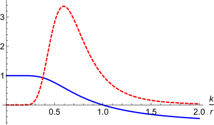
Figure 1: $\phi(r)/\eta$ (solid) and $(k/\eta)^{2}\mathcal{H}(r)$ (dashed) vs $k/r$ with $k/R=1$.

The total configuration energy (mass), $\mathcal{M}=\int d^{3}x\sqrt{g}\mathcal{H}=4\pi\mathcal{E}$, is given by

$$\mathcal{M}(R) =4\pi\lambda^{2}\int dr\frac{1}{r^{2}}(\eta^{2}-\phi^{2})^{2}=4\pi\lambda^{2}\eta^{4}\int_{0}^{\infty}dr\frac{1}{r^{2}}\text{sech}^{4}\Big{(}\frac{k}{r}-\frac{k}{R}\Big{)}$$

$$=\frac{4\pi k\eta^{2}}{3}\Big{[}2+3\tanh\Big{(}\frac{k}{R}\Big{)}-\tanh^{3}\Big{(}\frac{k}{R}\Big{)}\Big{]}$$ (38)

The total mass of the bubble $\mathcal{M}(R)$ decreases monotonically with $R$. This might lead one to assume that the bubble would tend to expand radially to decrease its mass, but the stability arguments, including the fact that $T_{rr}=0$, indicate otherwise. A bubble that is initially formed with a radius $R$ maintains that radius, and larger bubbles will be less massive. This is opposite to the case of a spherical bubble formed from a standard domain wall with a canonical potential $U(\phi)\sim g^{2}(\eta^{2}-\phi^{2})^{2}$ with no explicit $r$ dependence. In the standard type of scenario the bubble experiences a radially inward force due to the surface tension, causing it to collapse. Therefore, without some stabilizing mechanism, the solution $\phi=\phi(r,t)$ must be time dependent.

It can be noted that these results essentially duplicate those found in Ref.Bazeia PRD18 for the source field $\phi(r)$ of a magnetic monopole with internal structure. That is, the spherical shell $\phi(r)$ serves as the source field of a monopole for the model in Bazeia PRD18 . Additionally, these results basically reproduce those obtained for the scalar field in Ref.Bazeia ppt20 regarding electrically charged solitonic structures.

(2) Schwarzschild $\phi^{4}$ bubble:  Consider a spherical scalar field configuration centered on a black hole with a Schwarzschild radius $r_{S}$ in a Schwarzschild spacetime with metric described by

$$ds^{2}=\left(1-\frac{r_{S}}{r}\right)dt^{2}-\left(1-\frac{r_{S}}{r}\right)^{-1}dr^{2}-r^{2}(d\theta^{2}+\sin^{2}\theta d\varphi^{2})$$ (39)

In this case we have

$$f(r)=r^{2},\ \ \ h(r)=A(r)=\left(1-\frac{r_{S}}{r}\right),\ \ \ \ f^{2}(r)h(r)=r^{4}A=r^{4}\left(1-\frac{r_{S}}{r}\right)$$ (40)

Again, let’s choose a $\phi^{4}$ potential with

$$X(\phi)=-\lambda(\eta^{2}-\phi^{2}),\ \ \ \ V(r,\phi)=\frac{1}{2f^{2}(r)h(r)}X^{2}(\phi)=\frac{\lambda^{2}A^{-1}(r)}{2r^{4}}(\eta^{2}-\phi^{2})^{2}$$ (41)

With (27), $\int\frac{d\phi}{X(\phi)}=\int\frac{dr}{f(r)h(r)}$ gives $\int\frac{d\phi}{(\eta^{2}-\phi^{2})}=\lambda\int\frac{A^{-1}(r)\ }{r^{2}}dr$, so that,

$$\frac{\phi(r)}{\eta}=\psi(r)=\tanh\left[K\ln A(r)\right],\ \ \ (K=\frac{\lambda\eta}{r_{S}})$$ (42)

where the integration constant has been set to zero in this case and $K\equiv\lambda\eta/r_{S}$. The function $\psi(r)$ is a finite, bounded function of $r$, with $\psi(r)$ defined for $r\in(r_{S},\infty)$, with $\psi\rightarrow 0$ as $r\rightarrow\infty$ (Fig2). The energy density $\mathcal{H}=T_{0}^{0}$ is $\mathcal{H}(r,\phi)=\frac{A^{-1}(r)}{f^{2}(r)}X^{2}(\phi)=\frac{A^{-1}}{r^{4}}X^{2}$, i.e.,

$$\mathcal{H}=\frac{A^{-1}}{r^{4}}X^{2}(r)=A^{-1}r^{-4}B(1-\psi^{2})^{2},\ \ \ (B=\lambda^{2}\eta^{4})$$ (43)

The energy density is finite for all $r\geq r_{S}$ (i.e., outside the Schwarzschild horizon), with a maximum beyond $r_{S}$, and $\mathcal{H}\rightarrow 0$ as $r\rightarrow\infty$ (Fig2).

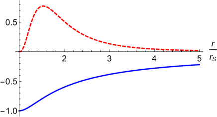
Figure 2: Sketches of $\phi(r)/\eta$ (solid) and $r_{S}^{4}\mathcal{H}(r)$ (dashed) vs $r/r_{S}$ with $B=10$.

The total energy (mass) of this scalar field configuration is $\mathcal{M}=\int_{r_{S}}^{\infty}d^{3}x\sqrt{g}\mathcal{H}(r)$. Using $\sqrt{g}=r^{2}\sin\theta$ gives

$$\mathcal{M}=4\pi\int_{r_{S}}^{\infty}\mathcal{H}(r)\ r^{2}dr=\frac{8\pi B}{3Kr_{S}}=\frac{8\pi\lambda^{2}\eta^{4}}{3Kr_{S}}=\frac{8\pi\lambda\eta^{3}}{3}$$ (44)

(3) Cosmic string background:  Here, the spacetime metric sourced by a straight cosmic string along the $z$ axis is described by Gott ApJ85 ,Hiscock PRD85 ,Aryal PRD86 ,Trenda EJP

$$ds^{2}=dt^{2}-dr^{2}-b^{2}r^{2}d\varphi^{2}-dz^{2}$$ (45)

where $b=(1-4G\mu)$ with $\mu$ being the mass per unit length of the string, and $\varphi\in[0,2\pi)$. (One can also define $\varphi^{\prime}=b\varphi$ with $\varphi^{\prime}\in[0,2\pi b)$. For $b=1$ we have a flat spacetime.) In this case

$$f(r)=\sqrt{g}=br,\ \ h(r)=B^{-1}(r)=A(r)=1$$ (46)

We again choose a $\phi^{4}$ potential, and define $\psi(r)=\phi(r)/\eta$,

$$X(\phi)=-\lambda(\eta^{2}-\phi^{2})=-\lambda\eta^{2}(1-\psi^{2}),\ \ \ \ V(r,\phi)=\frac{1}{2f^{2}h}X^{2}=\frac{\lambda^{2}}{2b^{2}r^{2}}(\eta^{2}-\phi^{2})^{2}$$ (47)

From (27) we obtain

$$\psi(r)=\frac{(\rho^{-2\alpha}-1)}{(\rho^{-2\alpha}+1)},\ \ \ \rho\equiv\frac{r}{r_{0}},\ \ \ (\alpha\equiv\frac{\lambda\eta}{b})$$ (48)

where $r_{0}$ is an integration constant. We have $\mathcal{H}=T_{0}^{0}=-\mathcal{L}=\frac{1}{2}h(\partial_{r}\phi)^{2}+V=\frac{1}{f^{2}h}X^{2}(\phi)$, or

$$\mathcal{H}=T_{0}^{0}=\frac{1}{b^{2}r^{2}}X^{2}=\frac{\beta}{\rho^{2}}(1-\psi^{2})^{2},\ \ \ \beta=\Big{(}\frac{\lambda^{2}\eta^{2}}{b^{2}}\Big{)}\frac{\eta^{2}}{r_{0}^{2}}=\frac{\alpha^{2}\eta^{2}}{r_{0}^{2}}$$

The functions $\psi$ and $\mathcal{H}$ are finite for all $\rho\in[0,\infty)$, with $\mathcal{H}$ maximizing at some finite radius with $\rho=1$, locating a “wall” of the cylindrical shell (Fig3). The scalar field configuration has a finite energy/length $\Lambda$ given by

$$\Lambda=2\pi br_{0}^{2}\int_{0}^{\infty}\mathcal{H}(\rho)\rho d\rho=\frac{8\pi b\beta r_{0}^{2}}{3\alpha}$$ (49)

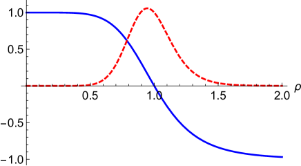
Figure 3: Sketches of $\phi(\rho)/\eta$ (solid) and $\mathcal{H}(\rho)/\beta$ (dashed) vs $\rho$.

Again, we can notice that the results obtained here for a cylindrical shell in flat spacetime ($b=1$) appear to be in agreement with those found in Ref Bazeia PRR19 for the source field $\chi(r)$ for multilayered vortices. This shell of a neutral scalar field is responsible for the structure of a vortex. The results reported here are also in apparent agreement with those of Ref. Bazeia ppt20 .

(4) Wormhole background:  Next, consider a scalar field $\phi(r)$ in the background spacetime of an Ellis-Bronnikov-Morris-Thorne wormhole Ellis ,Bronnikov ,M-T . The wormhole metric is given by

$$ds^{2}=dt^{2}-dr^{2}-(r^{2}+a^{2})(d\theta^{2}+\sin^{2}\theta d\varphi^{2})$$ (50)

where $r\in(-\infty,\infty)$ and the parameter $a$ represents the “radius“ of the wormhole throat where $r=0$. For this case we have $\sqrt{g}=(r^{2}+a^{2})\sin\theta$, with

$$f(r)=(r^{2}+a^{2}),\ \ \ \ A=h=1$$ (51)

Again we choose a $\phi^{4}$ potential, with

$$X=\lambda(\eta^{2}-\phi^{2})=\lambda\eta^{2}(1-\psi^{2});\ \ \ V(r,\phi)=\frac{1}{2f^{2}h}X^{2}=\frac{\lambda^{2}(\eta^{2}-\phi^{2})^{2}}{2(r^{2}+a^{2})^{2}}$$ (52)

where $\psi(r)=\phi(r)/\eta$. We define the dimensionless radial variable $\rho\equiv r/a$ and the dimensionless constant $K=\lambda\eta/a$ so that

$$V(\rho,\psi)=\frac{K^{4}}{2\lambda^{2}}\frac{(1-\psi^{2})^{2}}{(\rho^{2}+1)^{2}}$$ (53)

Using (27), along with (51) and (52), then yields

$$\psi(\rho)=\tanh\left[K(\tan^{-1}\rho-\tan^{-1}\rho_{0})\right]$$ (54)

where $-K\tan^{-1}\rho_{0}$ is an integration constant, with $\rho_{0}=r_{0}/a$ representing the center of the scalar field cloud $\psi(\rho)$ where $\psi(\rho_{0})=0$.

The energy density is represented by $\mathcal{H}=T_{0}^{0}=\frac{1}{2}(\partial_{r}\phi)^{2}+V(r,\phi)$, which for ansatz solutions satisfying (26) becomes $\mathcal{H}=2V(r,\phi)$. From (53) and (54),

$$\mathcal{H}=T_{0}^{0}=\frac{K^{4}}{\lambda^{2}}\frac{(1-\psi^{2})^{2}}{(\rho^{2}+1)^{2}}$$ (55)

The functions $\psi(\rho)$ and $\mathcal{H}(\rho)$ are finite for all $\rho$, with $\mathcal{H}$ maximizing at $\rho_{0}$ where $\psi$ vanishes (Fig4).

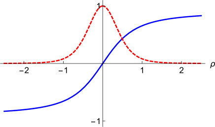
Figure 4: Sketches of $\psi(\rho)$ (solid) and $(\lambda^{2}/K^{4})\mathcal{H}(\rho)$ (dashed) vs $\rho$. The center of the cloud is chosen to be centered on the wormhole throat, $\rho_{0}=0$.

The mass $M$ of the scalar field configuration occupying the $r\geq 0$ region of the spacetime is

$$M=\int\mathcal{H}(r)\sqrt{g}d^{3}x=4\pi\int_{0}^{\infty}\mathcal{H}(r)(r^{2}+a^{2})dr=4\pi a^{3}\int_{0}^{\infty}\mathcal{H}(\rho)(\rho^{2}+1)d\rho$$ (56)

Using (54) and (55) then gives the result

$$M=\frac{4\pi a^{3}K^{3}}{3\lambda^{2}}\left[2+\text{sech}^{2}\frac{K\pi}{2}\tanh\frac{K\pi}{2}\right]$$ (57)

VI Summary

A set of scalar field potentials having the noncanonical form $U(r,\phi)=r^{-N}P(\phi)$, where $N\in\mathbb{Z}^{+}$ is a positive integer, and $P(\phi)=\frac{1}{2}W_{\phi}^{2}(\phi)$ with $W(\phi)$ a superpotential, was introduced in Ref. Bazeia PRL03 . Physical motivations include possible descriptions of effective potentials arising from other fields interacting with the scalar field $\phi$. Additionally, potentials of this form have been imposed in scalar field theories in order to produce field theoretic models with new and different features. This has proven to be of value in subsequent investigations of various models. (See, for example, Bazeia PRD18 -Bazeia ppt20 .) The function $U(r,\phi)$ is applicable to situations where there is a spherical symmetry in $D$ space dimensions of flat spacetimes, provided that $N$ and $D$ satisfy certain constraints.

Here, a new set of effective potentials is introduced, taking the general form $V(r,\phi)=F(r)P(\phi)$ where $F(r)=(f^{2}(r)h(r))^{-1}$ is a function of a radial coordinate $r$ (i.e., spherical or cylindrical symmetry) in a four dimensional spacetime, with $f(r)$ and $h(r)$ determined by the spacetime metric $g_{\mu\nu}$. (Specifically, $f(r)$ is the radial part of $\sqrt{g}$ and $h(r)=|g^{rr}|$.) The $\phi$ dependent part of the potential is given by $P(\phi)=\frac{1}{2}X^{2}(\phi)$, where $X(\phi)$ is a function taking the role of $W_{\phi}$. This form of potential $V(r,\phi)$ coincides with the potential $U(r,\phi)$ in the case of a flat four dimensional spacetime with spherical symmetry. Thus, at least in the case of four dimensions, the set of potentials $V(r,\phi)$ includes and generalizes the set of potentials $U(r,\phi)$ of Bazeia PRL03 . Both types of potentials are of interest from both physical and mathematical points of view, allowing stable, energy minimizing radial solutions derivable from a first order differential equation.

The utility of incorporating a potential $V(r,\phi)$ in a scalar field theory can be illustrated by using the method introduced by Atmaja and Ramadhan Atmaja PRD14 whereby the second order Euler-Lagrange equation of motion for $\phi(r)$ can be reduced to a first order Bogomol’nyi equation yielding a BPS type of minimal energy solution for the potential. Moreover, in Section 4 and the appendix, a general expression for the energy has been obtained, along with a proof, along the lines of Derrick’s theorem Derrick , that the solution $\phi(r)$ is radially stable. Examples of applying this method with potentials $V(r,\phi)$ have been provided in Section 5, which include using the ubiquitous symmetry breaking $\phi^{4}$ potential (where $X(\phi)=\lambda(\eta^{2}-\phi^{2})$) in background spacetimes (flat, Schwarzschild, cosmic string, and wormhole) with radial symmetry (spherical or cylindrical). The results of examples (1) and (3) presented here are seen to coincide with those of Bazeia PRD18 and Bazeia PRR19 for models describing magnetic monopoles with internal structure Bazeia PRD18 and multilayered vortices Bazeia PRR19 and charged solitons Bazeia ppt20 .

Appendix A Stability considerations

We consider 4D metrics with radial symmetry (spherical or cylindrical) of the form

$$\left\{\begin{array}[c]{ll}ds^{2}=A(r)dt^{2}-B(r)dr^{2}-R^{2}(r)(d\theta^{2}+\sin^{2}\theta d\varphi^{2}),&\text{(spherical symmetry) }\vskip 6.0pt plus 2.0pt minus 2.0pt\\ ds^{2}=A(r)dt^{2}-B(r)dr^{2}-\rho^{2}(r)d\varphi^{2}-\zeta^{2}(r)dz^{2},&\text{(cylindrical symmetry)}\end{array}\right.$$ (58)

in which case we have $\sqrt{g}=\sqrt{AB}R^{2}\sin\theta$ for spherical symmetry and $\sqrt{g}=\sqrt{AB}\rho\zeta$ for cylindrical symmetry Trenda EJP . (The functions $A(r)$ and $B(r)$ for the cylindrical case are generally different from those for the spherical case.) We represent the radial part of $\sqrt{g}$ by

$$f(r)=\sqrt{A(r)B(r)C(r)}$$ (59)

where $\sqrt{C(r)}$ is given by

$$\sqrt{C(r)}=\left\{\begin{array}[c]{ll}R^{2}(r),&\text{(spherical symmetry)\vskip 6.0pt plus 2.0pt minus 2.0pt}\\ \rho(r)\zeta(r),&\text{(cylindrical symmetry)}\end{array}\right.$$ (60)

Our ansatz for radially symmetric solutions is given by

$$\partial_{r}\phi =\frac{1}{f(r)h(r)}X(\phi),$$ (61a)

$$V(r,\phi) =\frac{1}{f^{2}(r)h(r)}P(\phi)=\frac{1}{2f^{2}(r)h(r)}X^{2}(\phi)$$ (61b)

where $h(r)\equiv|g^{rr}|=B^{-1}(r)$, and $P(\phi)=\frac{1}{2}X^{2}(\phi)$. The function $X(\phi)$ must be chosen to yield a finite energy (or finite energy per unit length) solution.

The energy of a spherically symmetric solution is

$$E=\int T_{0}^{0}\sqrt{g}d^{3}x=\Omega\int T_{0}^{0}f(r)dr$$ (62)

where $\Omega=\int d\Omega=\int\int\sin\theta d\theta d\varphi$. (The solid angle factor $\Omega$ takes a value of $4\pi$ in a flat spacetime, but may differ from $4\pi$ in spacetimes with a solid angular deficit or surplus.)

In the case of cylindrical symmetry, we can define the energy in a length $L$ along the $z$ direction as

$$E=\omega L\int T_{0}^{0}f(r)dr$$ (63)

where $\omega=\int d\varphi$. (We have $\omega=2\pi$ for a flat spacetime with no angular deficit or surplus.) For either case, let us define the quantity

$$\mathcal{E}=\left\{\begin{array}[c]{ll}\dfrac{E}{\Omega},\vskip 3.0pt plus 1.0pt minus 1.0pt&\text{(spherical symmetry)}\\ &\text{or}\\ \dfrac{E}{\omega L},&\text{(cylindrical symmetry)}\end{array}\right.$$ (64)

so that, in either case,

$$\mathcal{E}=\int T_{0}^{0}f(r)dr=\int\mathcal{H}f(r)dr$$ (65)

with $\mathcal{H}\equiv T_{0}^{0}$.

To investigate solution stability, we demand that $\mathcal{E}$ be finite, and that, furthermore, the solution considered represents a stable minimum for the energy. We follow the procedure used in Derrick’s theorem Derrick requiring that $\delta\mathcal{E}=0$ and $\delta^{2}\mathcal{E}\geq 0$ for a stable static solution that minimizes the action. To do so, we define $\phi_{\lambda}(r)=\phi(\lambda r)=\phi(r^{\prime})$, where $r^{\prime}=\lambda r$ with $\lambda$ being an arbitrary real parameter. We then define the energy parameter $\mathcal{E}_{\lambda}$ with $\phi(r)\rightarrow\phi_{\lambda}(r)$ in the energy integral. For stability, we require

$$\text{(i)\ \ }\frac{d\mathcal{E}_{\lambda}}{d\lambda}\Big{|}_{\lambda=1}\ =0$$ (66a)

$$\text{(ii)\ }\frac{d^{2}\mathcal{E}_{\lambda}}{d\lambda^{2}}\Big{|}_{\lambda=1} \geq 0$$ (66b)

Now, for any static, radially symmetric solution to the second order equation of motion $\square\phi+\partial_{\phi}V(r,\phi)=0$, for which $\mathcal{L}=\frac{1}{2}\partial^{r}\phi\partial_{r}\phi-V(r,\phi)$ and $\mathcal{H}=T_{0}^{0}=-g_{0}^{0}\mathcal{L}=-\mathcal{L}$, i.e., $\mathcal{H}=\frac{1}{2}h(\partial_{r}\phi)^{2}+V(r,\phi)$, where $V(r,\phi)$ is given by (61), the energy integral can be written as a sum of gradient plus potential contributions, $\mathcal{E}=I_{1}+I_{2}$:

$$\mathcal{E}=I_{1}+I_{2};\ \ \ \ \ I_{1}=\int\frac{1}{2}(\partial_{r}\phi)^{2}G(r)dr,\ \ \ I_{2}=\int P(\phi)H(r)dr$$ (67)

where we define $G=hf$, and $H=1/(fh)=G^{-1}$:

$$G(r)=hf=\sqrt{\frac{AC}{B}},\ \ \ H(r)=\frac{1}{hf}=\sqrt{\frac{B}{AC}}=G^{-1}(r)$$ (68)

Upon making the replacement $\phi\rightarrow\phi_{\lambda}$ we have $\mathcal{E}\rightarrow\mathcal{E}_{\lambda}=I_{1\lambda}+I_{2\lambda}$, with

$$\begin{array}[c]{ll}I_{1\lambda}&=\int\frac{1}{2}(\partial_{r}\phi_{\lambda})^{2}G(r)dr=\lambda\int\frac{1}{2}(\partial_{r^{\prime}}\phi_{\lambda})^{2}G(r)dr^{\prime}\equiv\lambda J_{1}(r)\\ I_{2\lambda}&=\int P(\phi_{\lambda})H(r)dr=\lambda^{-1}\int P(\phi_{\lambda})H(r)dr^{\prime}\equiv\lambda^{-1}J_{2}(r)\end{array}$$ (69)

The integrals $J_{1}$ and $J_{2}$ are functions of $r=\lambda^{-1}r^{\prime}$. Therefore, derivatives $\partial_{\lambda}J_{1,2}(r)=$ $\partial_{\lambda}J_{1,2}(\lambda^{-1}r^{\prime})$ involve $\partial_{\lambda}G(r)$ and $\partial_{\lambda}H(r)$, with $r=\lambda^{-1}r^{\prime}$, where

$$\frac{dG(r)}{d\lambda}=\frac{dG(r)}{dr}\frac{dr}{d\lambda}=-\lambda^{-2}r^{\prime}G^{\prime}(r),\ \ \ \frac{dH(r)}{d\lambda}=-\lambda^{-2}r^{\prime}H^{\prime}(r)$$ (70)

where we denote $G^{\prime}(r)=\partial_{r}G(r)$, $H^{\prime}(r)=\partial_{r}H(r)$.

Now using $\mathcal{E}_{\lambda}=I_{1\lambda}+I_{2\lambda}$ along with some straightforward (but a little tedious) algebra, we arrive at

$$\frac{d\mathcal{E}_{\lambda}}{d\lambda} =J_{1}-\lambda^{-1}K_{1}-\lambda^{-2}J_{2}-\lambda^{-3}Q_{1}$$ (71a)

$$\frac{d^{2}\mathcal{E}_{\lambda}}{d\lambda^{2}} =\lambda^{-3}K_{2}+2\lambda^{-3}J_{2}+4\lambda^{-4}Q_{1}+\lambda^{-5}Q_{2}$$ (71b)

where

$$\begin{array}[c]{ll}J_{1}=\int\frac{1}{2}(\partial_{r^{\prime}}\phi_{\lambda})^{2}G(r)dr^{\prime},&J_{2}=\int P(\phi_{\lambda})H(r)dr^{\prime}\\ K_{1}=\int\frac{1}{2}(\partial_{r^{\prime}}\phi_{\lambda})^{2}r^{\prime}G^{\prime}(r)dr^{\prime},&Q_{1}=\int P(\phi_{\lambda})r^{\prime}H^{\prime}(r)dr^{\prime}\\ K_{2}=\int\frac{1}{2}(\partial_{r^{\prime}}\phi_{\lambda})^{2}r^{\prime 2}G^{\prime\prime}(r)dr^{\prime},&Q_{2}=\int P(\phi_{\lambda})r^{\prime 2}H^{\prime\prime}(r)dr^{\prime}\end{array}$$ (72)

The objective is to evaluate (71) at $\lambda=1$ using (72) evaluated at $\lambda=1$ to verify the stability conditions (66) for all ansatz solutions satisfying (61), subject to the metric conditions of (58) - (60). For ansatz solutions satisfying the Bogomol’nyi equation (61a) with the potential (61b) it is found that $I_{1}=I_{2}$, i.e., the gradient and potential contributions to $\mathcal{E}=I_{1}+I_{2}$ are equal. Furthermore, setting $\lambda=1$ for the integrals of (72) simply amounts to setting $r^{\prime}=r$. In that case, it turns out to be convenient to re-express the integrals $J_{1}$, $K_{1}$, and $K_{2}$, when evaluated at $\lambda=1$, in terms of $P(\phi)$ and the function $G(r)$. Specifically, using $\frac{1}{2}(\partial_{r}\phi)^{2}G(r)=P(\phi)H(r)$

$$\begin{array}[c]{ll}J_{1}\rightarrow\int(PH^{2})Gdr,&J_{2}=\int PHdr\\ K_{1}\rightarrow\int(PH^{2})rG^{\prime}dr,&Q_{1}=\int P\ rH^{\prime}dr\\ K_{2}\rightarrow\int(PH^{2})r^{2}G^{\prime\prime}dr,&Q_{2}=\int P\ r^{2}H^{\prime\prime}(r)dr\end{array}$$ (73)

where $P=P(\phi)$, $G=G(r)$, $H=H(r)$, etc.

Now evaluating (71a) at $\lambda=1$ and enforcing (66a) gives

$$\frac{d\mathcal{E}}{d\lambda}\Big{|}_{\lambda=1} =(J_{1}-K_{1}-J_{2}-Q_{1})|_{\lambda=1}=(I_{1}-I_{2})|_{\lambda=1}-(K_{1}+Q_{1})|_{\lambda=1}=0$$

$$\implies(K_{1}+Q_{1})|_{\lambda=1}=0$$ (74)

In fact, using

$$H=G^{-1},\ \ H^{\prime}=-G^{-2}G^{\prime},\ \ \ H^{\prime\prime}=2G^{-3}G^{\prime 2}-G^{-2}G^{\prime\prime}$$ (75)

one can see that $K_{1}+Q_{1}=\int P\ r(H^{2}G^{\prime}+H^{\prime})dr=0$, i.e., $\dfrac{d\mathcal{E}}{d\lambda}\Big{|}_{\lambda=1}$ vanishes identically.

Next, an evaluation of (71b) at $\lambda=1$ gives

$$\frac{d^{2}\mathcal{E}_{\lambda}}{d\lambda^{2}}\Big{|}_{\lambda=1}=(K_{2}+2J_{2}+4Q_{1}+Q_{2})|_{\lambda=1}$$ (76)

Using the integrals in (73) produces

$$\frac{d^{2}\mathcal{E}_{\lambda}}{d\lambda^{2}}\Big{|}_{\lambda=1}=\int P(\phi)\left[(r^{2}H^{2}G^{\prime\prime})+(2H)+(4rH^{\prime})+(r^{2}H^{\prime\prime})\right]dr$$ (77)

Upon using (75) with a little algebra, this can be reduced to

$$\frac{d^{2}\mathcal{E}_{\lambda}}{d\lambda^{2}}\Big{|}_{\lambda=1}=\int P(\phi)G^{-3}\beta(r)dr$$ (78)

where

$$\beta(r)=r^{2}G^{\prime 2}-2rGG^{\prime}+G^{2}=(rG^{\prime}-G)^{2}\geq 0$$ (79)

Since $P(\phi)G^{-3}(r)\beta(r)\geq 0$ for any ansatz solution, we have the condition of (66b) being automatically satisfied, $\partial_{\lambda}^{2}\mathcal{E}_{\lambda}|_{\lambda=1}\geq 0$. We then conclude that for any radially symmetric ansatz solution with finite energy (or finite energy per unit length) in a spacetime with a metric of the form given by (58), the radial stability of the solution (i.e., stability against spontaneous radial expansion or collapse), as required by (66), is guaranteed.

In addition, we can take notice of the vanishing of the radial tension $T_{r}^{r}$ for the ansatz solutions for both the spherical and cylindrical symmetries:

$$T_{r}^{r}=\partial^{r}\phi\partial_{r}\phi-g_{r}^{r}\mathcal{L=-}\frac{1}{2}h(\partial_{r}\phi)^{2}+V(r,\phi)=0$$ (80)

This also indicates a stability against spontaneous radial expansion or contraction.

References

- (1) D. Bazeia, J. Menezes, R. Menezes, “New global defect structures”, Phys. Rev. Lett. 91 (2003) 241601 • e-Print: hep-th/0305234 [hep-th]
- (2) G.H. Derrick, “Comments on nonlinear wave equations as models for elementary particles”, J. Math. Phys. 5 (1964) 1252-1254
- (3) D. Bazeia, M. A. Marques, R. Menezes, “Magnetic monopoles with internal structure”, Phys. Rev. D 97 (2018) 10, 105024 • e-Print: 1805.03250 [hep-th]
- (4) D. Bazeia, M. A. Liao, M. A. Marques, R. Menezes, “Multilayered Vortices”, Phys. Rev. Research 1, 033053 (2019), • e-Print: 1908.07871 [hep-th]
- (5) J. Andrade, R. Casana, E. da Hora, C. dos Santos, “First-order solitons with internal structures in an extended Maxwell-CP(2) model”, Phys. Rev. D 99 (2019) 5, 056014 • e-Print: 1901.05094 [hep-th]
- (6) R. Casana, A. C. Santos, M. L. Dias, “BPS solitons with internal structure in the gauged O(3) sigma model”, Phys. Rev. D 102 (2020) 8, 085002 • e-Print: 2006.16466 [hep-th]
- (7) D. Bazeia, M. A. Marques, R. Menezes, “Electrically charged localized structures”, Eur. Phys. J. C 81 (2021) 1, 94 • e-Print: 2011.01766 [physics.gen-ph]
- (8) J. A. Gonzalez, D. Sudarsky, “Scalar solitons in a four-dimensional curved space-time”, Rev. Mex. Fis. 47 (2001) 231-233 • e-Print: gr-qc/0102061 [gr-qc]
- (9) L. Perivolaropoulos, “Gravitational Interactions of Finite Thickness Global Topological Defects with Black Holes”, Phys. Rev. D 97 (2018) 12, 124035 • e-Print: 1804.08098 [gr-qc]
- (10) G. Alestas, L. Perivolaropoulos, “Evading Derrick’s theorem in curved space: Static metastable spherical domain wall”, Phys. Rev. D 99 (2019) 6, 064026 • e-Print: 1901.06659 [gr-qc]
- (11) S. Carloni, J. L. Rosa, “Derrick’s theorem in curved spacetime”, Phys. Rev. D 100 (2019) 2, 025014 • e-Print: 1906.00702 [gr-qc]
- (12) B. Hartmann, G. Luchini, C. P. Constantinidis, C. F. S. Pereira, “Real scalar field kinks and antikinks and their perturbation spectra in a closed universe”, Phys. Rev. D 101 (2020) 7, 076004 • e-Print: 1908.09684 [hep-th]
- (13) G. Alestas, G.V. Kraniotis, L. Perivolaropoulos, “Existence and stability of static spherical fluid shells in a Schwarzschild-Rindler–anti–de Sitter metric”, Phys. Rev. D 102 (2020) 10, 104015 • e-Print: 2005.11702 [gr-qc]
- (14) A. N. Atmaja, H. S. Ramadhan, “Bogomol’nyi equations of classical solutions”, Phys. Rev. D 90 (2014) 10, 105009 • e-Print: 1406.6180 [hep-th]
- (15) C. Adam, F. Santamaria, “The First-Order Euler-Lagrange equations and some of their uses”, JHEP 12 (2016) 047 • e-Print: 1609.02154 [hep-th]
- (16) A. N. Atmaja, H. S. Ramadhan, E. da Hora, “More on Bogomol’nyi equations of three-dimensional generalized Maxwell-Higgs model using on-shell method”, JHEP 02 (2016) 117 • e-Print: 1505.01241 [hep-th]
- (17) T. Damour, G. Esposito-Farese, “Nonperturbative strong field effects in tensor - scalar theories of gravitation”, Phys.Rev.Lett. 70 (1993) 2220-2223
- (18) C.A.R. Herdeiro, T. Ikeda, M. Minamitsuji, T. Nakamura, E. Radu, “Spontaneous scalarization of a conducting sphere in Maxwell-scalar models”, Phys.Rev.D 103 (2021) 4, 044019 • e-Print: 2009.06971 [gr-qc]
- (19) C. S. Trendafilova, S. A. Fulling, “Static solutions of Einstein’s equations with cylindrical symmetry”, Eur. J. Phys. 32 (2011) 1663-1677 • e-Print: 1101.4668 [gr-qc]
- (20) J. R. Gott, III, “Gravitational lensing effects of vacuum strings: Exact solutions”, Astrophys. J. 288 (1985) 422-427
- (21) W. A. Hiscock, “Exact Gravitational Field of a String”, Phys. Rev. D 31 (1985) 3288-3290
- (22) M. Aryal, L. H. Ford, A. Vilenkin, “Cosmic Strings and Black Holes”, Phys. Rev. D 34 (1986) 2263
- (23) H. G. Ellis, “Ether flow through a drainhole - a particle model in general relativity”, J. Math. Phys. 14 (1973) 104-118
- (24) K. A. Bronnikov, “Scalar-tensor theory and scalar charge”, Acta Phys. Polon. B 4 (1973) 251-266
- (25) M. S. Morris, K. S. Thorne, “Wormholes in space-time and their use for interstellar travel: A tool for teaching general relativity”, Am. J. Phys. 56 (1988) 395-412