Randomization-based Test for Censored Outcomes: A New Look at the Logrank Test

Abstract

Two-sample tests with censored outcomes are a classical topic in statistics with wide use even in cutting edge applications. There are at least two modes of inference used to justify two-sample tests. One is usual superpopulation inference assuming that units are independent and identically distributed (i.i.d.) samples from some superpopulation; the other is finite population inference that relies on the random assignments of units into different groups. When randomization is actually implemented, the latter has the advantage of avoiding distributional assumptions on the outcomes. In this paper, we focus on finite population inference for censored outcomes, which has been less explored in the literature. Moreover, we allow the censoring time to depend on treatment assignment, under which exact permutation inference is unachievable. We find that, surprisingly, the usual logrank test can also be justified by randomization. Specifically, under a Bernoulli randomized experiment with non-informative i.i.d. censoring, the logrank test is asymptotically valid for testing Fisher’s null hypothesis of no treatment effect on any unit. The asymptotic validity of the logrank test does not require any distributional assumption on the potential event times. We further extend the theory to the stratified logrank test, which is useful for randomized block designs and when censoring mechanisms vary across strata. In sum, the developed theory for the logrank test from finite population inference supplements its classical theory from usual superpopulation inference, and helps provide a broader justification for the logrank test.

Keywords: Logrank test; Randomization; Non-informative censoring; Potential outcome; Stratified logrank test

Introduction

1.1 Superpopulation versus finite population inference

The two-sample test has been one of the most classical and important topics in statistics. Most theoretical justification for two-sample tests relies on the assumption of independent and identically distributed (i.i.d.) sampling of units from some population. However, in the context of randomized experiments, which are widely used in industry (e.g., Box et al. 2005; Dasgupta et al. 2015), clinical trials (e.g., Rosenberger and Lachin 2015), and more recently in social science (e.g., Athey and Imbens 2017) and technology companies (e.g., Basse et al. 2019; Bojinov and Shephard 2019; Bojinov et al. 2020), it is often more natural to conduct inference based on randomization of the treatment assignments. This is often called randomization-based or design-based inference, as well as finite population inference (Fisher 1935; Neyman 1923). Specifically, under finite population inference, each unit’s potential outcome (Neyman 1923; Rubin 1974) under either treatment is viewed as a fixed constant (or equivalently being conditioned on), and the randomness in the observed data comes solely from the physical randomization of treatment assignments, which acts as the “reasoned basis” for inference (Fisher 1935).

Compared to superpopulation inference, finite population inference has the following two advantages. First, finite population inference focuses explicitly on the experimental units by conditioning on their potential outcomes, which in some sense makes our inference more relevant for the units in hand. On the contrary, the superpopulation inference assumes that the units are i.i.d. samples from an often hypothetical superpopulation, and focuses on inference about the superpopulation distribution. Second, the validity of superpopulation inference generally relies crucially on the i.i.d. sampling of units. However, the validity of finite population inference relies on the randomization of treatment assignments, which can be guaranteed by design, and does not require the units’ potential outcomes to be either independent or identically distributed. Therefore, finite population inference can avoid distributional assumptions on the units and thus provides inference procedures with broader justifications, at least in the context of randomized experiments. For a more detailed comparison between these two types of inference, see, e.g., Little (2004) with an emphasis on survey sampling, Rosenbaum (2002, Chapter 2.4.5) with an emphasis on causal inference and Abadie et al. (2020) with an emphasis on regression analysis.

1.2 Two-sample tests for censored outcomes

In many clinical trials, the primary outcome is time to a certain event. The outcome may be censored, rendering the usual two-sample tests inapplicable. In the presence of censoring, Gehan (1965) proposed a permutation test using a generalized Wilcoxon statistic, and Mantel (1966) proposed the logrank test by combining the Mantel–Haenszel statistics for all contingency tables during the study period. Prentice (1978) extended the two tests to more general linear rank tests. Aalen (1978) and Gill (1980) provided a full and rigorous study of the asymptotic properties of these tests. Most theoretical justifications for these two-sample tests have assumed that the units are i.i.d. samples from some superpopulation (Fleming and Harrington 1991). However, this i.i.d. assumption can be violated when the units’ outcomes are inhomogeneous or dependent on each other due to some (hidden) risk factors. For example, in a multicenter clinical trial, each patient’s outcome may depend on his/her own characteristics such as age and sex, and the outcomes for patients within the same center may be correlated due to the same environment or other center-specific factors (Cai et al. 1999).

There have been fewer studies of two-sample tests for censored outcomes under finite population inference. To test Fisher’s null hypothesis of no treatment effect for any unit, Rosenbaum (2002) proposed randomization tests for censored outcomes using a partial ordering, and Zhang and Rosenberger (2005) established asymptotic Normality of the randomization distribution of the logrank statistic. Both approaches require the assumption of identical potential censoring times under treatment and control. Under this identical censoring assumption, Fisher’s null hypothesis is sharp, the null distributions of test statistics (e.g., logrank statistic) are known exactly, and the asymptotics provides mainly a numerical approximation. However, as Zhang and Rosenberger (2005) commented, the assumption of identical censoring can be violated due to toxicity or a side effect of either treatment. When the censoring times can be different under the two treatment arms, Fisher’s null hypothesis of no effect becomes composite. In this case, understanding the randomization distribution of the logrank statistic becomes more challenging, and in the meanwhile more critical for inference, because the exact randomization distribution is no longer known.

1.3 Our contribution

Neyman (1923) first studied the randomization distribution of the difference-in-means statistic under finite population inference, and provided an asymptotic valid test for a non-sharp null hypothesis, for which no exact permutation tests are available and large-sample approximations become essential. In particular, he showed that the classical $t$-test is still asymptotically valid under randomization, although in a generally conservative way. In the presence of censoring where the censoring can depend on the treatment, Fisher’s null is composite, and there has not been any test available that can be justified by randomization. As Zhang and Rosenberger (2005) commented, it does not appear that randomization-based techniques can be used to perform the analysis. In this paper, we will show that it is still possible to conduct randomization-based tests in large samples, and our approach is based on the logrank test, one of the most popular two-sample tests for censored outcomes.

From Neyman (1923), test statistics that are justified under i.i.d.  sampling from a superpopulation can sometimes also be justified under randomization of a finite population (Ding 2017). However, this is not always true (see, e.g., Freedman 2008a, b, c). Our question is, can the logrank test for studying censored time-to-event outcomes be justified under randomization of a finite population?

We will show that as long as the censoring is non-informative and the potential censoring times are i.i.d. across all units, the logrank test can be justified by randomization, without requiring any distributional assumption on the potential event times. Specifically, under a Bernoulli randomized experiment and non-informative i.i.d. censoring, if the treatment has no effect on any unit’s event time, then the randomization distribution of the logrank statistic, i.e., the distribution conditional on all the potential event times, is asymptotically standard Gaussian. Our proof makes use of a novel martingale construction, the martingale central limit theorem, and Gaussian approximation of hypergeometric distributions. Our result shows that in practice we can be more confident in using the logrank test, when the units are randomly assigned to the two treatment arms and the censoring is i.i.d. across units under each treatment arm. The result is particularly useful if the experimenter is able to control both the treatment assignment and the censoring mechanisms, because the logrank test can then be justified by physical implementation.

Furthermore, we extend the theory to the stratified logrank test. Note that under superpopulation inference, the stratified logrank test is often preferred when we want to adjust covariates that may affect the event times. Because our finite-population justification of the logrank test allow arbitrary distribution of the event times, the original motivation for stratification seems unnecessary, at least in terms of the validity of the logrank test. However, as demonstrated later, such an extension is still useful, especially in randomized block designs and when the censoring mechanism varies across strata.

The paper proceeds as follows. Section 2 introduces the potential outcome framework, and briefly reviews the superpopulation and finite population inference. Section 3 reviews usual superpopulation inference for the logrank test, and Section 4 compares it to finite population inference by simulation. Section 5 studies the exact randomization distribution of the logrank statistic, and Section 6 studies its large-sample approximation. Section 7 conducts simulations to investigate violation of assumptions, and motivates the stratified logrank test. Section 8 studies the stratified logrank test. Section 9 concludes with a short discussion.

Framework, notation and assumptions

2.1 Potential event/censoring time and treatment assignment

We consider an experiment on $n$ units with two treatment arms: an active treatment and a control. The outcome of interest is the time to a pre-specified event, e.g., occurrence of a certain disease or death. Under the potential outcome framework, for each unit $i$, let $T_{i}(1)$ and $T_{i}(0)$ denote the potential event times under treatment and control, respectively. Let $\bm{T}(1)=(T_{1}(1),\ldots,T_{n}(1))^{\prime}$ and $\bm{T}(0)=(T_{1}(0),\ldots,T_{n}(0))^{\prime}$ be the vectors of potential event times for all $n$ units under treatment and control, respectively. The treatment effects are then characterized by the comparison between potential outcomes $\bm{T}(1)$ and $\bm{T}(0)$.

Under either treatment arm, we may not be able to observe the event time due to censoring, which itself may be related to the treatment. We introduce $C_{i}(1)$ and $C_{i}(0)$ to denote the potential censoring times for unit $i$ under treatment and control, respectively. Let $\bm{C}(1)=(C_{1}(1),\ldots,C_{n}(1))^{\prime}$ and $\bm{C}(0)=(C_{1}(0),\ldots,C_{n}(0))^{\prime}$ be the vectors of all units’ potential censoring times under treatment and control, respectively. Both the $T_{i}(z)$’s and $C_{i}(z)$’s are nonnegative for $z=0,1$. If $C_{i}(z)=\infty$, then there is no censoring for unit $i$ under treatment arm $z$. We say a unit is at risk if its event has not happened and it has not been censored. For $z=0,1,$ $W_{i}(z)=\min\{T_{i}(z),C_{i}(z)\}$ is then the potential time at risk for unit $i$ under treatment arm $z$, and $\Delta_{i}(z)=\mathbbm{1}\{T_{i}(z)\leq C_{i}(z)\}$ is the corresponding potential event indicator.

Let $Z_{i}\in\{0,1\}$ be the treatment assignment for unit $i$, which equals 1 if unit $i$ receives the active treatment and 0 otherwise, and $\bm{Z}=(Z_{1},\ldots,Z_{n})^{\prime}$ be the treatment assignment vector for all units. Then $T_{i}=Z_{i}\cdot T_{i}(1)+(1-Z_{i})\cdot T_{i}(0)$ and $C_{i}=Z_{i}\cdot C_{i}(1)+(1-Z_{i})\cdot C_{i}(0)$ are the realized event and censoring times for unit $i$. Note that these realized variables, $T_{i}$ and $C_{i}$, may not be observed in practice. Instead, for each unit $i$, we can observe only the minimum of the realized event and censoring times, or equivalently the time at risk, i.e., $W_{i}=\min\{T_{i},C_{i}\}=Z_{i}W_{i}(1)+(1-Z_{i})W_{i}(0)$, and the corresponding event indicator for whether the realized event happens before censoring, i.e., $\Delta_{i}=\mathbbm{1}(T_{i}\leq C_{i})=Z_{i}\Delta_{i}(1)+(1-Z_{i})\Delta_{i}(0).$

To facilitate the discussion and ease understanding, we list all the notation with a short explanation in Table 1, and introduce the Studies of Left Ventricular Dysfunction (SOLVD, The SOLVD Investigators 1990) as an illustrative example. The SOLVD is an extensive research program that contains a double-blinded randomized trial conducted in 23 medical centers. The trial entrolled 2569 eligible patients, and randomly assigned about half of them to receive enalapril or placebo. The patients were followed up for 41.4 months on average. Suppose that the event of interest is death; see The SOLVD Investigators (1991) and Cai et al. (1999) for other events of interest. Then in our notation, $Z$ denotes the treatment indicator for whether the patient receives enalapril or placebo, $T(1)$ and $T(0)$ denote the potential survival times under treatment and control, and $C(1)$ and $C(0)$ denote the potential follow-up times under treatment and control.

Table 1: Notation and explanation.

Notation	Explanation
$Z$	treatment assignment indicator
$T(z)$	potential event time under treatment arm $z$
$C(z)$	potential censoring time under treatment arm $z$
$W(z)=\min\{Y(z),C(z)\}$	potential time at risk under treatment arm $z$
$\Delta(z)=\mathbbm{1}\{T_{i}(z)\leq C_{i}(z)\}$	potential event indicator under treatment arm $z$
$T,C,W,\Delta$	realized event time, censoring time, time at risk and event indicator
$t_{1}<t_{2}<\ldots<t_{K}$	distinct values of the control potential event times $\{T_{i}(0):1\leq i\leq n\}$
$d_{k}=\sum_{i=1}^{n}\mathbbm{1}(T_{i}(0)=t_{k})$	number of units potentially having events at time $t_{k}$ under control
$n_{k}=\sum_{i=1}^{n}\mathbbm{1}(T_{i}(0)\geq t_{k})$	number of units potentially having events no earlier than time $t_{k}$ under control
$h_{k}=d_{k}/n_{k}$	hazard at time $t_{k}$ for all units under control
$F(\cdot),\lambda(\cdot),\Lambda(\cdot)$	survival, hazard and integrated hazard functions for empirical distribution of $T_{i}(0)$

2.2 Treatment assignment and censoring mechanisms

We study finite population inference in the presence of censoring, where both $T_{i}(1)$’s and $T_{i}(0)$’s are viewed as fixed constants. This is equivalent to conducting inference conditioning on all the potential event times $\bm{T}(1)$ and $\bm{T}(0)$. Consequently, the inference relies crucially on the randomness of the treatment assignments as well as potential censoring times. In the following, we will write the conditioning on $(\bm{T}(1),\bm{T}(0))$ explicitly to emphasize that all the potential event times are viewed as fixed constants. On the contrary, in usual superpopulation inference, the units’ potential event times $(T_{i}(1),T_{i}(0))$’s are assumed to be i.i.d. samples from some distribution, the treatment assignments are conditioned on and thus viewed as constants, and the inference relies crucially on the randomness of the potential event times. To ease understanding, we review and compare the superpopulation and finite population inferences for the classical two-sample $t$-test when there is no censoring; see Section 2.4.

Under finite population inference, because the potential event times $\bm{T}(1)$ and $\bm{T}(0)$ have been conditioned on or equivalently viewed as constants, the randomness in the observed data $W_{i}$’s and $\Delta_{i}$’s comes solely from the random treatment assignments $Z_{i}$’s and the random censoring times $C_{i}(1)$’s and $C_{i}(0)$’s. Therefore, the distributions of the treatment assignments and the potential censoring times govern the data-generating process and are crucial for statistical inference. First, we consider the distribution of $\bm{Z}$, also called the treatment assignment mechanism. We focus on the Bernoulli randomized experiment with equal probability of receiving active treatment for all units. Let $\text{Bern}(p)$ denote a Bernoulli distribution that has probability $p$ at 1 and $1-p$ at 0, for $p\in(0,1)$.

Assumption 1.

Conditional on all the potential event and censoring times, the treatment assignments are i.i.d. across all units, i.e.,

$$Z_{i}\mid\bm{T}(1),\bm{T}(0),\bm{C}(1),\bm{C}(0)\ \overset{\text{i.i.d.}}{\sim}\ \text{Bern}(p_{1}),\quad(1\leq i\leq n)$$

for some $p_{1}\equiv 1-p_{0}\in(0,1).$

Second, we consider the distribution of $(\bm{C}(1),\bm{C}(0))$, also called the censoring mechanism. We focus on the case of non-informative i.i.d. censoring.

Assumption 2.

The potential censoring times for all units are independent of the potential event times for all units, i.e., $(\bm{C}(1),\bm{C}(0))\begin{picture}(9.0,8.0)\put(0.0,0.0){\line(1,0){9.0}} \put(3.0,0.0){\line(0,1){8.0}} \put(6.0,0.0){\line(0,1){8.0}} \end{picture}(\bm{T}(1),\bm{T}(0)),$ and the $n$ two-dimensional random vectors, $(C_{1}(1),C_{1}(0))^{\prime},(C_{2}(1),C_{2}(0))^{\prime},$ $\ldots,$ $(C_{n}(1),C_{n}(0))^{\prime}$, are i.i.d.

Note that Assumption 2 does not require $C_{i}(1)$ and $C_{i}(0)$ for the same unit $i$ to be independent or identically distributed. Instead, $C_{i}(1)$ and $C_{i}(0)$ can have different marginal distributions and arbitrary dependence. Under Assumption 2, let $G_{z}(c)\equiv\text{pr}(C_{i}(z)\geq c)$ for $z=0,1$. In the context of the SOLVD, Assumption 2 assumes that the treatment and control potential follow-up times are i.i.d. across all units and importantly that they are independent of the potential survival times. It can be violated when the censoring is informative about the survival time. For example, in the SOLVD, the blinded medication may be terminated when the patient remains symptomatic despite maximum therapy with such medications (The SOLVD Investigators 1991), under which the censoring might indicate a shorter survival time; see also Leung et al. (1997) for more examples and discussions.

In our finite population inference, Assumptions 1 and 2 are crucial and in some sense necessary for justifying the logrank test or identifying the treatment effects. Note that we relax the i.i.d. assumption on the potential event times and allow them to be arbitrary constants. If, for instance, Assumption 2 fails and the potential censoring times are not identically distributed for all units, then the censoring times can be related to the event times in which case identification of the treatment effect is lost without further assumptions (Tsiatis 1975). We conduct a simulation study in Section 7 to investigate the violation of Assumptions 1 and 2, showing their necessity for the validity of the logrank test under finite population inference.

Finally, we give two technical remarks regarding the assumptions. First, we can weaken Assumptions 1 and 2 by allowing dependence between the treatment assignment and the potential censoring times, but we still require $(Z_{i},C_{i}(1),C_{i}(0))$’s to be i.i.d. and independent of the potential event times; see Appendix A1 of the the Supplementary Material for details. Second, similar assumptions are also invoked in usual superpopulation inference, but they can have weaker forms; see Appendix A2 of the Supplementary Material for a more detailed comparison.

2.3 Fisher’s null hypothesis of no treatment effect

We are interested in testing whether the treatment has any effect on the units’ event times. We consider Fisher’s null hypothesis (Fisher 1935) of no treatment effect on any unit:

$$H_{0}:\bm{T}(1)=\bm{T}(0).$$ (2.1)

In the absence of censoring, Fisher’s null $H_{0}$ is sharp in the sense that all the potential event times are known from the observed data. However, this is generally not true in the presence of censoring. For example, for a unit $i$ under control with $Z_{i}=0$, $\Delta_{i}=0$ and $W_{i}\geq 0$, under $H_{0}$, we know that $T_{i}(1)=T_{i}(0)>C_{i}(0)=W_{i}$, but we do not know the exact values of $T_{i}(1)$, $C_{i}(1)$, $W_{i}(1)$ and $\Delta_{i}(1)$ under the alternative treatment. The non-sharpness of $H_{0}$ implies that we cannot know the null distribution of the logrank statistic exactly, and the usual randomization or permutation tests may not be valid. To conduct valid inference, it is crucial to understand the null distribution of the logrank statistic under $H_{0}$, which generally depends on the treatment assignment and censoring mechanisms, as well as all the potential event times. Here the null distribution of the logrank statistic refers to its conditional distribution given $\bm{T}(1)$ and $\bm{T}(0)$ under Fisher’s null $H_{0}$.

2.4 Superpopulation and finite population inferences

We give a brief comparison between superpopulation and finite population inferences using the classical two-sample $t$-test as an illustration. Such a comparison may help the reader understand the difference between these two types of inference, and make the purpose of the paper less obscure. We refer the reader to Abadie et al. (2020) for a more comprehensive comparison.

Suppose that there is no censoring and the realized event times $T_{i}$’s can always be observed. Let $\mathfrak{T}$ denote the two-sample $t$-statistic calculated from $(Z_{i},T_{i})$’s. Assume that the treatment assignments are completely randomized and Fisher’s null $H_{0}$ in (2.1) holds. Below we discuss two types of justification for the asymptotic Gaussianity of $\mathfrak{T}$. First, under the superpopulation inference, the potential event times $T_{i}(1)=T_{i}(0)$’s are assumed to be i.i.d. samples from some distribution. Under certain regularity conditions and conditional on the treatment assignments, the $t$-statistic is asymptotically standard Gaussian, in the sense that $\mathfrak{T}\mid\bm{Z}\stackrel{{\scriptstyle d}}{{\longrightarrow}}\mathcal{N}(0,1).$ Second, under the finite population inference, all the potential event times are viewed as fixed constants or equivalently being conditioned on. Under certain regularity conditions and conditional on the potential event times, the $t$-statistic is asymptotically standard Gaussian (Neyman 1923; Hájek 1960; Li and Ding 2017), in the sense that $\mathfrak{T}\mid\bm{T}(1),\bm{T}(0)\stackrel{{\scriptstyle d}}{{\longrightarrow}}\mathcal{N}(0,1).$

Although leading to similar conclusions justifying the two-sample $t$-test, the superpopulation and finite population inferences are quite different. The main difference comes from the source of randomness. The distribution of $\mathfrak{T}$ under the superpopulation setting is conditioning on the treatment assignment $\bm{Z}$, and the randomness comes solely from the random potential event times $\bm{T}(1)$ and $\bm{T}(0)$. However, the distribution of $\mathfrak{T}$ under finite population setting is conditioning on the potential event times $\bm{T}(1)$ and $\bm{T}(0)$, and the randomness comes solely from the random treatment assignment $\bm{Z}$. Moreover, for the asymptotics, these two types of inference impose different forms of regularity conditions. The superpopulation asymptotics imposes regularity conditions on the population distribution that generates the i.i.d. samples, while the finite population asymptotics imposes regularity conditions directly on the fixed potential event times. The regularity conditions for finite population inference does not, at least explicitly, require the potential event times $T_{i}(0)$’s to be either identically distributed or independent, and can be weaker than that for superpopulation inference (Li and Ding 2017). Therefore, intuitively, finite population inference can give a broader justification for the two-sample $t$-test in randomized experiments. We also conduct a simulation study to confirm this intuition; see Appendix A3 of the Supplementary Material.

Two-sample logrank test under usual superpopulation inference

As discussed in Section 2.4, randomization justifies the usual two-sample $t$-test, without any distributional assumption on the potential event times. However, the methods that are valid under the superpopulation inference cannot always be justified by randomization under finite population inference. For example, Freedman (2008a, b, c) showed that randomization may not justify linear or logistic regression. In this paper, we investigate whether randomization can justify the logrank test without requiring any distributional assumption on the potential event times. We first briefly review usual superpopulation inference for the logrank test.

For any time $t\geq 0$, let

$$\overline{N}_{1}(t)=\sum_{i=1}^{n}Z_{i}\mathbbm{1}(W_{i}\geq t),\quad\overline{N}_{0}(t)=\sum_{i=1}^{n}(1-Z_{i})\mathbbm{1}(W_{i}\geq t),$$

$$\overline{N}(t)=\overline{N}_{1}(t)+\overline{N}_{0}(t)=\sum_{i=1}^{n}\mathbbm{1}(W_{i}\geq t)$$

be the numbers of units at risk at time $t$ in treated, control and both groups, respectively. Let

$$\overline{D}_{1}(t)=\sum_{i=1}^{n}Z_{i}\Delta_{i}\mathbbm{1}(W_{i}=t),\quad\overline{D}_{0}(t)=\sum_{i=1}^{n}(1-Z_{i})\Delta_{i}\mathbbm{1}(W_{i}=t),$$

$$\overline{D}(t)=\overline{D}_{1}(t)+\overline{D}_{0}(t)=\sum_{i=1}^{n}\Delta_{i}\mathbbm{1}(W_{i}=t)$$

be the numbers of units having events at time $t$ in treated, control and both groups, respectively. In the context of the SOLVD, $\overline{N}_{1}(t)$, $\overline{N}_{0}(t)$ and $\overline{N}(t)$ denote the numbers of units that are still alive and under follow-up at time $t$ in treated, control and both groups, and $\overline{D}_{1}(t)$, $\overline{D}_{0}(t)$ and $\overline{D}(t)$ denote the numbers of units that die at time $t$ in treated, control and both groups. These quantities constitute the contingency table at time $t$, as shown in Table 2.

Table 2: The contingency table at time $t$

Group	Having event	Not having event	Total
Treatment	$\overline{D}_{1}(t)=\sum_{i=1}^{n}Z_{i}\Delta_{i}\mathbbm{1}(W_{i}=t)$	$\overline{N}_{1}(t)-\overline{D}_{1}(t)$	$\overline{N}_{1}(t)=\sum_{i=1}^{n}Z_{i}\mathbbm{1}(W_{i}\geq t)$
Control	$\overline{D}_{0}(t)=\sum_{i=1}^{n}(1-Z_{i})\Delta_{i}\mathbbm{1}(W_{i}=t)$	$\overline{N}_{0}(t)-\overline{D}_{0}(t)$	$\overline{N}_{0}(t)=\sum_{i=1}^{n}(1-Z_{i})\mathbbm{1}(W_{i}\geq t)$
Total	$D(t)=\sum_{i=1}^{n}\Delta_{i}\mathbbm{1}(W_{i}=t)$	$N(t)-D(t)$	$N(t)=\sum_{i=1}^{n}\mathbbm{1}(W_{i}\geq t)$

Under Fisher’s null $H_{0}$ in (2.1) and usual superpopulation formulation, the units’ potential event times $T_{i}(1)=T_{i}(0)$’s are i.i.d. samples from a superpopulation. Suppose the treatment assignment $\bm{Z}$, the potential even times $(\bm{T}(1),\bm{T}(0))$, and the potential censoring times $(\bm{C}(1),\bm{C}(0))$ are mutually independent. Then conditional on the treatment assignment $\bm{Z}$, the realized event times $(T_{i},C_{i})$’s follow the usual random censorship model (Fleming and Harrington 1991). For any $t\geq 0$, Mantel (1966) observed that, conditional on the margins of Table 2, the number of observed events in treated group follows a hypergeometric distribution:

$$\overline{D}_{1}(t)\mid\bm{Z},\overline{N}_{1}(t),\overline{N}_{0}(t),\overline{D}(t)\ \sim\ \text{HGeom}(\overline{N}(t),\overline{D}(t),\overline{N}_{1}(t)),$$ (3.1)

with mean and variance

$$\overline{M}(t)=\frac{\overline{D}(t)\overline{N}_{1}(t)}{\overline{N}(t)},\quad\overline{V}(t)=\frac{\overline{D}(t)\{\overline{N}(t)-\overline{D}(t)\}\overline{N}_{1}(t)\overline{N}_{0}(t)}{\{\overline{N}(t)\}^{2}\{\overline{N}(t)-1\}},$$ (3.2)

where we use $\text{HGeom}(m,k,b)$ to denote the hypergeometric distribution that describes the probability of $x$ successes in $b$ draws, without replacement, from a finite population of size $m$ with exactly $k$ successes, for any integers $m,k$ and $b$ with $0\leq k,b\leq m$. The denominators in (3.2) can be zero when $\overline{N}(t)$ equals 0 or 1, making $\overline{M}(t)$ or $\overline{V}(t)$ undefined. For descriptive convenience, we define $0/0$ as 0. This is reasonable because when the denominator of $\overline{V}(t)$ is zero, the numerator must be zero and $\overline{D}_{1}(t)$ is a constant equal to $\overline{M}(t)$ with zero variance. Below we give some intuition for the hypergeometric distribution in (3.1). For any unit at risk at time $t$, no matter whether it received treatment or control (i.e., in Row 1 or 2 of Table 2), it has the same probability to have or not to have the event (i.e., in Column 1 or 2 of Table 2). This is because the probability of immediately having an event (i.e., hazard) for any unit at risk at time $t$ under either treatment arm is the same, a fact implied by the i.i.d. assumptions on the potential event times and their independence of the treatment assignments and potential censoring times. Similar to Fisher’s exact test, conditioning on all the margins of Table 2, the number of treated units having events at time $t$ follows a hypergeometric distribution as in (3.1).

The logrank statistic is then defined as the summation of the differences between the observed and expected event counts in treated group over all time (Mantel 1966), i.e., $\sum_{t}\{\overline{D}_{1}(t)-\overline{M}(t)\}$. To conduct the logrank test, we will first estimate its standard deviation and then compare the logrank statistic standardized by its estimated standard deviation to standard Gaussian quantiles. Here we consider the commonly used variance estimator $\sum_{t}\overline{V}(t)$; see, e.g., Brown (1984) for other choice of variance estimator. The standardized logrank statistic is then

$$\text{LR}=\left\{\sum_{t}\overline{V}(t)\right\}^{-1/2}\sum_{t}\left\{\overline{D}_{1}(t)-\overline{M}(t)\right\}.$$ (3.3)

For convenience, in the following we will simply call the standardized logrank statistic in (3.3) as the logrank statistic. Because $\overline{D}_{1}(t)-\overline{M}(t)$ and $\overline{V}(t)$ are nonzero only if $\overline{D}(t)>0$, the summations in (3.3) only need to be taken over the observed event times. When the potential event times $T_{i}(1)=T_{i}(0)$’s are i.i.d. from a superpopulation, from the classical theory for the logrank test, LR in (3.3) is asymptotically standard Gaussian under some regularity conditions:

$$\text{LR}\mid\bm{Z}\stackrel{{\scriptstyle d}}{{\longrightarrow}}\mathcal{N}(0,1);$$ (3.4)

see Appendix A2 of the Supplementary Material for more detailed discussion, and Aalen (1978); Gill (1980) and Fleming and Harrington (1991) for rigorous justification using the counting process formulation and martingale properties. The distribution (3.4) of LR is conditioning on the treatment assignments, and relies crucially on the random potential event times. In simple words, the treatment assignments are fixed, and the potential event times are random.

A simulation study of the logrank test under both superpopulation and finite population inferences

We conduct a simulation study for the logrank test from both the superpopulation and finite population perspectives, with possibly non-identically distributed and dependent potential event times. Specifically, we will show that, with non-identically distributed or correlated potential event times $T_{i}(1)=T_{i}(0)$’s across units, the conditional distribution of the logrank statistic given treatment assignments from the superpopulation perspective can be quite different from the standard Gaussian distribution, while the conditional distribution given the potential event times from the finite population perspective can be close to the standard Gaussian distribution. This implies that the finite population inference can give a broader justification for the classical logrank test.

Table 3: Parameter values for different super population settings

Case	$\rho$	$\theta$	Dependence	Heterogeneity
1	$0$	$0$	No	No
2	$0.5$	$0$	Yes	No
3	$0$	$1$	No	Yes
4	$0.5$	$1$	Yes	Yes

For any $\rho\in(-1,1)$, let $\bm{\Sigma}_{\rho}\in\mathbb{R}^{n\times n}$ be a correlation matrix whose $(i,j)$th element is $\rho^{|i-j|}$. A random vector $(\eta_{1},\eta_{2},\ldots,\eta_{n})^{\prime}\in\mathbb{R}^{n}$ is said to follow a Gaussian copula with correlation matrix $\bm{\Sigma}_{\rho}$ if $(\Phi^{-1}(\eta_{1}),\ldots,$ $\Phi^{-1}(\eta_{n}))^{\prime}\sim\mathcal{N}(0,\bm{\Sigma}_{\rho})$, where $\Phi^{-1}(\cdot)$ denotes the quantile function of the standard Gaussian distribution. We can verify that the marginal distributions of the $\eta_{i}$’s are all uniform on $(0,1)$, and thus the $-\log(1-\eta_{i})$’s all follow the exponential distribution with rate parameter 1, denoted by $\text{Expo}(1)$. For $1\leq i\leq n$, we introduce a binary $X_{i}$ to denote some pretreatment covariate of unit $i$. We consider the following model for the potential event times:

$$T_{i}(1)=T_{i}(0)=-\log(1-\eta_{i})\cdot\left(1+\theta X_{i}\right),\quad(1\leq i\leq n)$$ (4.1)

$$(\eta_{1},\eta_{2},\ldots,\eta_{n})\sim\text{Gaussian copula with correlation matrix }\bm{\Sigma}_{\rho},$$

$$\bm{X}\equiv(X_{1},\ldots,X_{n})=(\underbrace{0,0,\ldots,0}_{0.2\times n},\underbrace{1,1,\ldots,1}_{0.3\times n},\underbrace{0,0,\ldots,0}_{0.3\times n},\underbrace{1,1,\ldots,1}_{0.2\times n}).$$

In model (4.1), the potential event times marginally follow scaled exponential distributions, with the scales depending on the parameter $\theta$ and the covariates $X_{i}$’s, and their dependence structure is determined by the parameter $\rho$. The covariates $X_{i}$’s in (4.1) are fixed constants, or equivalently we can view (4.1) as a model conditional on the $X_{i}$’s. We consider four choices of the parameters $(\theta,\rho)$ as in Table 3, which determine the existence of heterogeneity and dependence among the units’ potential event times. For the potential censoring times, we generate them as i.i.d. samples from the following model:

$$C_{i}(1)\sim 2\cdot\text{Expo}(1),\ C_{i}(0)\sim\text{Expo}(1),\ C_{i}(1)\begin{picture}(9.0,8.0)\put(0.0,0.0){\line(1,0){9.0}} \put(3.0,0.0){\line(0,1){8.0}} \put(6.0,0.0){\line(0,1){8.0}} \end{picture}C_{i}(0),\quad(1\leq i\leq n)$$ (4.2)

where the censoring time tends to be larger under treatment than under control. For the treatment assignments, we consider the following generating model:

$$Z_{1},Z_{2},\ldots,Z_{n}\ \overset{\text{i.i.d.}}{\sim}\ \text{Bern}(0.5).$$ (4.3)

Furthermore, the potential event times $\bm{T}(1)=\bm{T}(0)$ in (4.1), the potential censoring times $(\bm{C}(1),\bm{C}(0))$ in (4.2), and the treatment assignment $\bm{Z}$ in (4.3) are mutually independent. Throughout the paper, under each simulation scenario, the sample size $n$ equals $1000$, and the number of simulated datasets equals $10^{4}$.

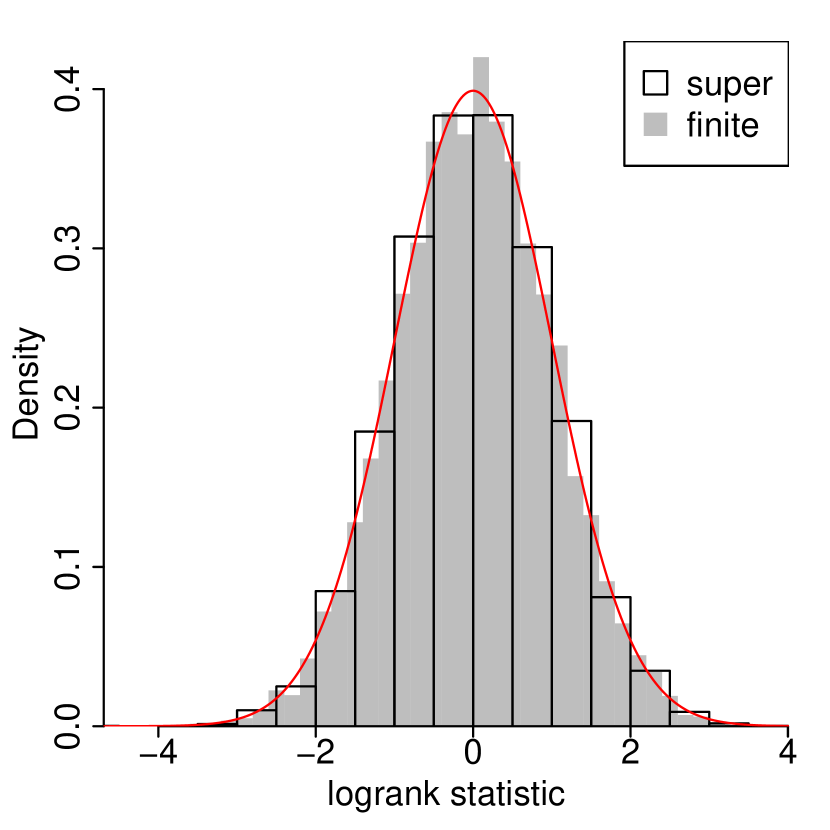
case 1

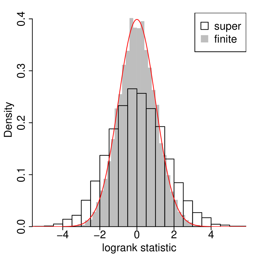
case 2

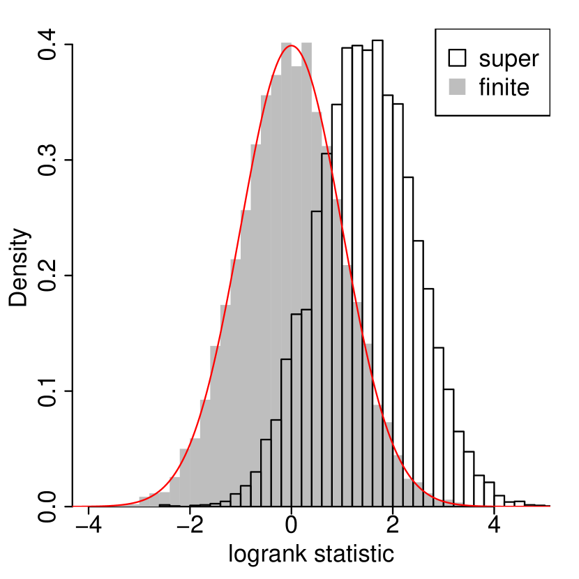
case 3

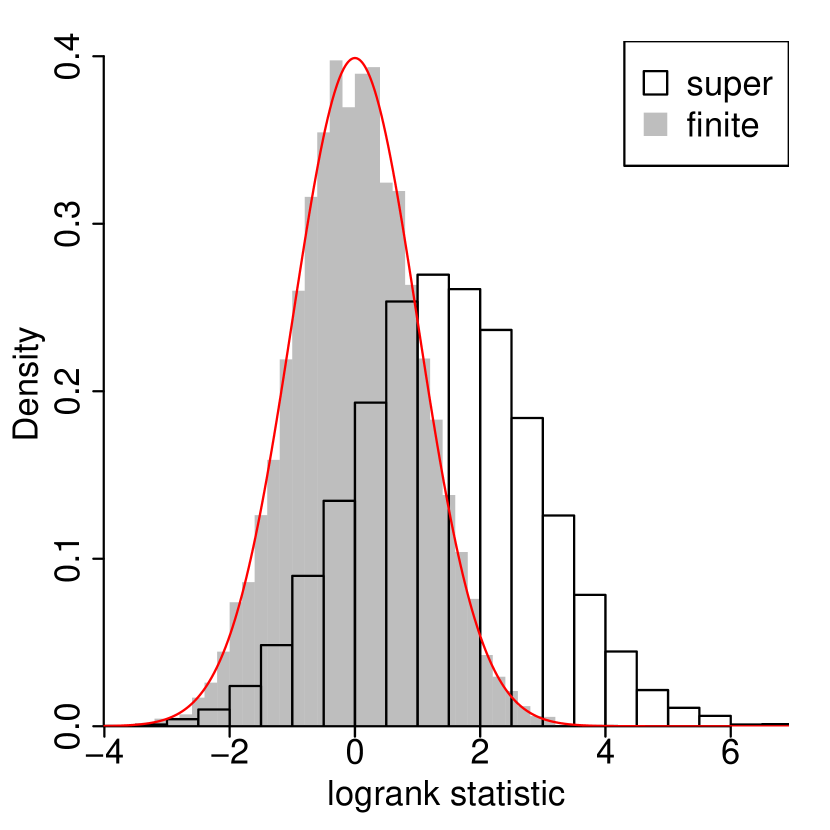
case 4

Figure 1: Histograms of the logrank statistic in the superpopulation and finite population settings with parameter values in the four cases of Table 3. The white histograms denote the distributions of the logrank statistic under the superpopulation setting with random potential event times and fixed treatment assignments, and the gray histograms denote the distributions of the logrank statistic under finite population setting with fixed potential event times and random treatment assignments. The red lines denote the density of a standard Gaussian distribution.

First, we mimic the superpopulation inference conditioning on the treatment assignment. We fix the treatment assignment $\bm{Z}$ as the following constant vector:

$$\bm{Z}=(\underbrace{1,1,\ldots,1}_{n/2},\underbrace{0,0,\ldots,0}_{n/2})^{\prime},$$ (4.4)

and generate random potential event times $(\bm{T}(1),\bm{T}(0))$ and random potential censoring times $(\bm{C}(1),\bm{C}(0))$ from models (4.1) and (4.2), respectively. The resulting distribution of the logrank statistic is then LR conditional on the treatment assignment $\bm{Z}$ in (4.4). In Figure 1, the four white histograms show the distributions of the logrank statistic under the four cases in Table 3. When there exist dependence or heterogeneity among units’ potential event times, the conditional distribution of LR given $\bm{Z}$ in (4.4) is no longer close to a standard Gaussian distribution.

Second, we mimic finite population inference conditioning on the potential event times. We fix the potential event times as one realization from model (4.1):

$$\bm{T}(1)=\bm{T}(0)=\text{a realization from model \eqref{eq:model_potential_outcome}},$$ (4.5)

and generate random potential censoring times $(\bm{C}(1),\bm{C}(0))$ and random treatment assignment $\bm{Z}$ from (4.2) and (4.3), respectively. The resulting distribution of the logrank statistic is then LR conditional on $\bm{T}(1)=\bm{T}(0)$ in (4.5). In Figure 1, the four gray histograms show the distributions of the logrank statistic under the four cases in Table 3 or equivalently four different realizations of the potential event times. From Figure 1, they are all close to a standard Gaussian distribution.

Third, we consider the scenario where all potential event times, potential censoring times and treatment assignments are randomly generated from (4.1), (4.2) and (4.3), respectively. The resulting distribution of the logrank statistic can be viewed as the conditional distribution of LR given $\bm{T}(1)$ and $\bm{T}(0)$ marginalizing over all potential event times. From the finite population simulation, we expect the distribution of LR to be close to a standard Gaussian distribution. This is confirmed by Figure A3 in the Supplementary Material.

From the simulation, randomization justifies the logrank test, without requiring distributional assumptions (such as i.i.d.) on the potential event times. In the remainder of the paper, we will study explicitly the conditional distribution of LR given all the potential event times, and prove its asymptotic Gaussianity under certain regularity conditions.

Randomization distribution of the logrank statistic

In this section, we study the randomization distribution of the logrank statistic under the finite population inference, where the potential event times are being conditioned on or equivalently viewed as fixed constants, i.e., $\text{LR}\mid\bm{T}(1),\bm{T}(0)$. Below we first introduce some finite population quantities depending only on the potential event times, which are also summarized in Table 1. For the potential event times under control, we use $t_{1}<\ldots<t_{K}$ to denote distinct values in $\{T_{i}(0):1\leq i\leq n\}$, where $K$ is the total number of distinct event times. Let $d_{k}=\sum_{i=1}^{n}\mathbbm{1}(T_{i}(0)=t_{k})$ be the number of units potentially having events at time $t_{k}$, $n_{k}=\sum_{i=1}^{n}\mathbbm{1}(T_{i}(0)\geq t_{k})$ be the number of units potentially having events no earlier than time $t_{k}$, and $h_{k}=d_{k}/n_{k}$ be the hazard at time $t_{k}$. We introduce $F(\cdot)$ to denote the empirical survival distribution for the control potential event times, i.e., $F(t)=n^{-1}\sum_{i=1}^{n}\mathbbm{1}\{T_{i}(0)\geq t\}$. Then, by definition, $F(t)=1=n_{1}/n$ when $t\leq t_{1}$, $F(t)=n_{k}/n$ when $t_{k-1}<t\leq t_{k}$, for $2\leq k\leq K$, and $F(t)=0$ when $t>t_{K}$. Consequently, the hazard function for the distribution $F(\cdot)$ is $\lambda(t)$, which takes value $h_{k}$ when $t=t_{k}$ for $1\leq k\leq K$ and zero otherwise, and the corresponding integrated hazard function is $\Lambda(t)=\sum_{k:t_{k}\leq t}h_{k}.$

5.1 Contingency tables under randomization

We first investigate the contingency table at time $t$ (i.e., Table 2) under finite population inference. The treatment assignment $\bm{Z}$, instead of being conditioned on as in Section 3, plays an important role in inducing randomness of the quantities in Table 2. As demonstrated in Appendix A4 of the Supplementary Material, for any unit at risk at time $t$, no matter whether it had an event or not (i.e., in Column 1 or 2 of Table 2), it has the same probability of receiving treatment or control (i.e., in Row 1 or 2 of Table 2). The mutual independence among $(Z_{i},W_{i},\Delta_{i})$’s under Assumptions 1 and 2 then implies that, conditional on the margins of Table 2, $\overline{D}_{1}(t)$ follows a hypergeometric distribution.

Theorem 1.

Under Assumptions 1 and 2 and the null hypothesis $H_{0}$ in (2.1), and conditioning on all the potential event times $\bm{T}(1)$ and $\bm{T}(0)$,

$$\overline{D}_{1}(t)\mid\bm{T}(1),\bm{T}(0),\overline{N}(t),\overline{D}(t),\overline{N}_{1}(t)\ \sim\ \text{HGeom}(\overline{N}(t),\overline{D}(t),\overline{N}_{1}(t)).$$ (5.1)

In the superpopulation setting in Section 3, the hypergeometric distribution (3.1) of the same form is justified by the i.i.d. potential event times with fixed treatment assignments. However, (5.1) in Theorem 1 is justified by the random treatment assignments with fixed potential event times. In particular, Theorem 1 does not impose any distributional assumption on the potential event times, and thus allows them to have unit-specific distributions and arbitrary dependence structure. Moreover, comparing the justification for hypergeometric distributions in (3.1) and (5.1), the former relies on the fact that units in either row of Table 2 have the same probability to fall in either column, while the latter relies on the fact that units in either column of Table 2 have the same probability to fall in either row. In simple words, one takes a row-wise perspective, while the other takes a column-wise perspective.

5.2 A martingale difference sequence representation

Recall that $\{t_{1},\ldots,t_{K}\}$ are the distinct values of all control potential event times. Under Fisher’s null $H_{0}$ in (2.1), the observed event times must be in the set $\{t_{1},\ldots,t_{K}\}$. Thus, the summations in (3.3) only need to be taken over $t_{1},t_{2},\ldots,t_{K}$. To facilitate the discussion, at each time $t_{k}$, we introduce

$$N_{1k}=\overline{N}_{1}(t_{k}),\quad N_{0k}=\overline{N}_{0}(t_{k}),\quad N_{k}=\overline{N}(t_{k}),\qquad(1\leq k\leq K)$$

to denote the numbers of units at risk in treated, control and both groups, and

$$D_{1k}=\overline{D}_{1}(t_{k}),\quad D_{0k}=\overline{D}_{0}(t_{k}),\quad D_{k}=\overline{D}(t_{k}),\qquad(1\leq k\leq K)$$

to denote the numbers of units having events in treated, control and both groups. Analogous to (3.2), for $1\leq k\leq K$, we further define

$$M_{k}=\overline{M}(t_{k})=\frac{D_{k}N_{1k}}{N_{k}},\quad V_{k}=\overline{V}(t_{k})=\frac{D_{k}(N_{k}-D_{k})N_{1k}N_{0k}}{N_{k}^{2}(N_{k}-1)}.$$

The overall observed-expected difference and the corresponding overall variance are, respectively,

$$L\equiv\sum_{k=1}^{K}(D_{1k}-M_{k})\ \ \ \text{and}\ \ \ U\equiv\sum_{k=1}^{K}V_{k}.$$ (5.2)

We can then rewrite the logrank statistic in (3.3) as

$$\text{LR}=\left(\sum_{k=1}^{K}V_{k}\right)^{-1/2}\sum_{k=1}^{K}(D_{1k}-M_{k})=U^{-1/2}L.$$ (5.3)

The difficulty in studying the distribution of (5.3) comes from the dependence among all the contingency tables at times $t_{1},\ldots,t_{K}$. Fortunately, as demonstrated shortly, the sequence of the observed-expected differences, $\{D_{1k}-M_{k}:k=1,\ldots,K\}$, is actually a martingale difference sequence. Define $t_{0}=-\infty$ and $t_{K+1}=\infty$ for descriptive convenience. For $0\leq k\leq K$, define a $\sigma$-algebra $\mathcal{F}_{k}$ as

$$\mathcal{F}_{k} =\sigma\left\{\mathbbm{1}(W_{i}\geq t_{q}),\Delta_{i}\mathbbm{1}(W_{i}=t_{q}),Z_{i}\Delta_{i}\mathbbm{1}(W_{i}=t_{q-1}),\vphantom{\sum_{j=1}^{n}Z_{j}\mathbbm{1}(W_{j}\geq t_{q})}\right.$$

$$\quad\ \left.\qquad\qquad\qquad\qquad\sum_{j=1}^{n}Z_{j}\mathbbm{1}(W_{j}\geq t_{q}),\quad 1\leq q\leq k+1,\ \ 1\leq i\leq n\right\}.$$

Intuitively, $\mathcal{F}_{k}$ contains the information of whether the units had events or were at risk up to time $t_{k+1}$, the treatment indicators for units having events up to time $t_{k}$, and the numbers of treated units at risk up to time $t_{k+1}$. We can verify that $\mathcal{F}_{k}$ contains the contingency tables up to time $t_{k}$, and margins of the contingency table at time $t_{k+1}$. Consequently, $D_{1k}$ is $\mathcal{F}_{k}$-measurable, and $(N_{k},D_{k},N_{1k})$ are $\mathcal{F}_{k-1}$-measurable. Moreover, the information in $\mathcal{F}_{k-1}$ other than $(N_{k},D_{k},N_{1k})$ does not change the conditional distribution of $D_{1k}$.

Theorem 2.

Under Assumptions 1 and 2 and the null hypothesis $H_{0}$ in (2.1), and conditioning on all the potential event times $\bm{T}(1)$ and $\bm{T}(0)$,

• $\{D_{1k}-M_{k}\}_{k=1}^{K}$ is a martingale difference sequence with respect to the filtration $\mathcal{F}_{k}$’s;

• conditional on $\mathcal{F}_{k-1}$, $D_{1k}$ follows a hypergeometric distribution with parameters $(N_{k},D_{k},N_{1k})$, i.e.,

  $$D_{1k}\mid\bm{T}(1),\bm{T}(0),\mathcal{F}_{k-1}\ \sim\ \text{HGeom}(N_{k},D_{k},N_{1k}).$$

Theorem 2 implies that $L$ in (5.2) is a summation of a martingale difference sequence. This is similar to usual superpopulation inference, where $L$ is related to integrals with respect to martingales. Under both finite population and superpopulation inferences, the martingale property plays a critical role in the large-sample asymptotic analyses. However, they are driven by different sources of randomness: the martingale property under finite population inference relies on the random treatment assignments, while that under the superpopulation inference relies on the random potential event times. Martingale properties driven by random treatment assignments have also been utilized in settings with sequentially assigned treatments over time; see, e.g., recent work of Bojinov and Shephard (2019) and Papadogeorgou et al. (2020).

Below we investigate the first two moments of the randomization distribution of the observed-expected difference $L$ in (5.2). Let $G(t)=p_{1}G_{1}(t)+p_{0}G_{0}(t)$ be the survival function of the realized censoring time $C_{i}$, $g_{k}=G(t_{k})$ be the probability that the realized censoring time $C_{i}$ is no less than $t_{k}$, and $\phi_{k}=p_{1}G_{1}(t_{k})/G(t_{k})$ be the conditional probability of receiving active treatment given that the realized censoring time is no less than $t_{k}$.

Theorem 3.

Under Assumptions 1 and 2 and the null hypothesis $H_{0}$ in (2.1), and conditioning on all the potential event times $\bm{T}(1)$ and $\bm{T}(0)$, the observed-expected difference $L$ in (5.2) has mean 0, i.e., $\mathbb{E}\{L\mid\bm{T}(1),\bm{T}(0)\}=0$, and it has variance

$$\quad\ \text{Var}\left\{L\mid\bm{T}(1),\bm{T}(0)\right\}$$ (5.4)

$$=\mathbb{E}\left\{U\mid\bm{T}(1),\bm{T}(0)\right\}=\sum_{k=1}^{K}\mathbb{E}\left\{V_{k}\mid\bm{T}(0),\bm{T}(0)\right\}$$

$$=\sum_{k=1}^{K}\frac{n_{k}^{2}}{n_{k}-1}h_{k}(1-h_{k})\phi_{k}(1-\phi_{k})\left\{g_{k}-\frac{1-(1-g_{k})^{n_{k}}}{n_{k}}\right\}.$$

From Theorem 3, conditional on the potential event times, $U$ in (5.2) is an unbiased variance estimator for $L$, and thus LR in (5.3) is indeed a standardization of $L$. This is similar to the superpopulation setting that conditions on the treatment assignments. Below we further make a connection between the variance formula of $L$ in (5.4) and its asymptotic variance formula under the superpopulation inference. Recall that $F(\cdot)$ is the empirical survival distribution for the control potential event times $\{T_{i}(0):1\leq i\leq n\}$, and $\Lambda(\cdot)$ is the corresponding integrated hazard function. Ignoring the terms of order $n_{k}^{-1}$, we can simplify the variance formula in (5.4) as:

$$\quad\ \text{Var}\left\{L\mid\bm{T}(1),\bm{T}(0)\right\}$$

$$=\sum_{k=1}^{K}n_{k}\left(1+\frac{1}{n_{k}-1}\right)h_{k}(1-h_{k})\phi_{k}(1-\phi_{k})\left\{g_{k}-\frac{1-(1-g_{k})^{n_{k}}}{n_{k}}\right\}$$

$$\approx\sum_{k=1}^{K}n_{k}h_{k}(1-h_{k})\phi_{k}(1-\phi_{k})g_{k}$$

$$=np_{1}p_{0}\int_{0}^{\infty}F(t)\frac{G_{1}(t)G_{0}(t)}{p_{1}G_{1}(t)+p_{0}G_{0}(t)}\left\{1-\Delta\Lambda(t)\right\}\text{d}\Lambda(t),$$

which has the same form as the asymptotic variance of $L$ under usual superpopulation inference, except that the distribution $F$ is replaced by the population distribution of the potential event times. Therefore, we can view the variance formula (5.4) as a finite population analogue of the superpopulation variance formula. Importantly, the former is for the variance of LR given the potential event times, while the latter is for the variance of LR given the treatment assignments.

Asymptotic randomization distribution of the logrank statistic

The exact randomization distribution of the logrank statistic depends on all the potential event times and is thus generally intractable. In this section we study its large-sample approximation using only the first two moments. The finite population asymptotics embeds the units into a sequence of finite populations with increasing sizes, and studies the limiting distributions of certain statistics along this sequence of finite populations (Li and Ding 2017). Here we consider two cases depending on the total number of distinct potential event times. In the first case, the number of distinct potential event times goes to infinity as the sample size of the finite population goes to infinity; in the second case, the number of distinct potential event times is bounded. The first case is more reasonable when the event times are continuous, whereas the second case is more reasonable when the event times are discrete with a finite support.

6.1 A diverging number of distinct potential event times

We first consider the case in which the number of distinct potential event times $K$ goes to infinity as the sample size $n$ increases. Let

$$\tilde{d}=\max_{1\leq k\leq K}d_{k}=\max_{1\leq k\leq K}\left|\left\{i:T_{i}(0)=t_{k}\right\}\right|$$ (6.1)

be the maximum number of units potentially having events at the same time. We further introduce a random vector $(\tilde{C}_{i}(1),\tilde{C}_{i}(0))$ that shares the same marginal distributions as $(C_{i}(1),C_{i}(0))$ but has two independent components, i.e., $\tilde{C}_{i}(z)\sim C_{i}(z)$ for $z=0,1$ and $\tilde{C}_{i}(1)\begin{picture}(9.0,8.0)\put(0.0,0.0){\line(1,0){9.0}} \put(3.0,0.0){\line(0,1){8.0}} \put(6.0,0.0){\line(0,1){8.0}} \end{picture}\tilde{C}_{i}(0)$. The survival function of $\min\{\tilde{C}_{i}(1),\tilde{C}_{i}(0)\}$ is then $\tilde{G}(t)=G_{1}(t)G_{0}(t)$. Under Fisher’s null $H_{0}$ in (2.1), with the pseudo potential censoring times $\tilde{C}_{i}(1)$ and $\tilde{C}_{i}(0)$, we can observe unit $i$’s event no matter whether it is assigned to treatment or control if and only if $\min\{\tilde{C}_{i}(1),\tilde{C}_{i}(0)\}\geq T_{i}(1)=T_{i}(0)$. Thus, the expected proportion of units whose events can be observed under both treatment and control with the pseudo potential censoring times is

$$\tilde{g} \equiv\mathbb{E}\left[\frac{1}{n}\sum_{i=1}^{n}\mathbbm{1}\left\{\min\{\tilde{C}_{i}(1),\tilde{C}_{i}(0)\}\geq T_{i}(0)\right\}\right]=\frac{1}{n}\sum_{i=1}^{n}\tilde{G}(T_{i}(0))$$ (6.2)

$$=\frac{1}{n}\sum_{k=1}^{K}d_{k}\tilde{G}(t_{k}).$$

Here $\tilde{g}$ is defined in terms of the pseudo potential censoring times and may be different from that defined in terms of the original potential censoring times. Nevertheless, since we do not specify the distribution of $(C_{i}(1),C_{i}(0))$ and allow arbitrary dependence between them, $\tilde{g}$ is a quantity that can be realized when $C_{i}(1)$ and $C_{i}(0)$ are indeed independent. Note that both $\tilde{d}$ and $\tilde{g}$ in (6.1) and (6.2), as well as $p_{z}$ and $G_{z}(\cdot)$ for $z=0,1$, depend on the finite population of size $n$. For descriptive convenience, we make such dependence implicit. As shown in the following condition, the limiting behavior of $\tilde{d}$ and $\tilde{g}$ plays an important role in the asymptotic Gaussian approximation of the logrank statistic.

Condition 1.

Along the sequence of finite populations satisfying $H_{0}$ in (2.1), as $n\rightarrow\infty$, for $z=0,1$,

• the probability of receiving treatment arm $z$, $p_{z}$, has a positive limit;

• the maximum number of potentially simultaneous events $\tilde{d}$ in (6.1) and the expected proportion of observed events $\tilde{g}$ in (6.2) satisfy

  $$\frac{\tilde{g}}{\tilde{d}}\min\left\{\left(\frac{n}{\log n}\right)^{1/2},\frac{n}{\tilde{d}^{2}}\right\}=\min\left\{\frac{\tilde{g}}{\tilde{d}}\left(\frac{n}{\log n}\right)^{1/2},\frac{\tilde{g}n}{\tilde{d}^{3}}\right\}\stackrel{{\scriptstyle}}{{\longrightarrow}}\infty.$$ (6.3)

Under finite population inference, the potential event times are being conditioned on or equivalently viewed as fixed constants. Consequently, Condition 1 imposes conditions on all the potential event times directly. This is different from regularity conditions under superpopulation inference, which are usually on the population distribution that generates the i.i.d. units. Specifically, Condition 1 involves $p_{z}$ for the treatment assignment mechanism, $\tilde{d}$ in (6.1) that is a deterministic function of the potential event times, and $\tilde{g}$ in (6.2) that is determined by both the potential event times and the censoring mechanism. These quantities are fixed and can vary with sample size $n$, and Condition 1 imposes some constraints on their limiting behavior as $n$ goes to infinity. Note that $\tilde{g}\leq 1$ and $\tilde{d}\geq 1$. Condition 1 implies that $K\geq n/\tilde{d}\rightarrow\infty$ as $n\rightarrow\infty$, i.e., the number of distinct potential event times goes to infinity as $n\rightarrow\infty$.

Below we give some intuition for Condition 1, showing that the regularity conditions there are rather weak. In Condition 1, (i) is a natural requirement, and we investigate (ii) when units are i.i.d. samples from a superpopulation. Assume that the potential event times $T_{i}(1)=T_{i}(0)$’s are i.i.d. samples from a superpopulation with continuous distribution, and the distribution of potential censoring times $(C_{i}(1),C_{i}(0))$ is the same along the sequence of finite populations. If the minimum of the pseudo potential censoring times has a positive probability to be no less than the potential event time, i.e., $\mathbb{E}\{\tilde{G}(T_{i}(0))\}=\mathbb{E}\{G_{1}(T_{i}(0))G_{0}(T_{i}(0))\}>0,$ then as $n\rightarrow\infty$, with probability one, $\tilde{d}=1$, $\tilde{g}$ has a positive limit, and (ii) in Condition 1 holds.

The theorem below shows that Condition 1 is sufficient for the asymptotic standard Gaussianity of the logrank statistic LR in (5.3).

Theorem 4.

Under Assumptions 1 and 2 and the null hypothesis $H_{0}$ in (2.1), and conditioning on all the potential event times, if Condition 1 holds, then $U$ is a consistent variance estimator for $L$ in (5.2), i.e.,

$$\frac{U}{\text{Var}\left\{L\mid\bm{T}(1),\bm{T}(0)\right\}}\mid\bm{T}(1),\bm{T}(0)\ \stackrel{{\scriptstyle p}}{{\longrightarrow}}\ 1,$$

and the logrank statistic $\text{LR}=U^{-1/2}L$ in (5.3) is asymptotically standard Gaussian, i.e.,

$$\text{LR}\mid\bm{T}(1),\bm{T}(0)\ \stackrel{{\scriptstyle d}}{{\longrightarrow}}\ \mathcal{N}(0,1).$$ (6.4)

The asymptotic Gaussianity in Theorem 4 is established using the martingale central limit theorem (Hall and Heyde 1980). In particular, the first term in (6.3) guarantees the consistency of the variance estimator $U$, and the second term in (6.3) guarantees the conditional Lindeberg condition. Moreover, although (3.4) and (6.4) lead to the same asymptotic distribution for the logrank statistic, they rely on different sources of randomness. Specifically, the asymptotics in (3.4) relies on the random potential event times that are assumed to be i.i.d. from some population while fixing the treatment assignments. On the contrary, the asymptotics in (6.4) relies on the random treatment assignments that can be physically implemented while fixing the potential event times, which are then allowed to have arbitrary dependence and heterogeneity across units. Therefore, Theorem 4, or more generally finite population inference, can sometimes provide a broader justification for the logrank test compared to usual superpopulation inference. This is also confirmed by the simulation results in Section 4.

6.2 A bounded number of distinct potential event times

We now consider the case in which the number of distinct potential event times $K$ is bounded as the sample size $n$ increases. Without loss of generality, we assume that $K$ is fixed along the sequence of finite populations, because we can always add several distinct event times with no units potentially having events at those times. When $K$ is fixed, for a specific time $t_{k}$, if (i) there are non-negligible proportions of units receiving both treatment and control, (ii) the potential censoring times under both treatment and control have positive probabilities to be no less than $t_{k}$, and (iii) there are non-negligible proportions of units potentially having events both at time $t_{k}$ and later than $t_{k}$, then we expect that all margins of the contingency table at time $t_{k}$, $(N_{1k},N_{0k},D_{k},N_{k}-D_{k})$, as well as the conditional variance $V_{k}$, go to infinity as the sample size $n$ goes to infinity. The property of hypergeometric distributions then enables us to establish the Gaussian approximation for $V_{k}^{-1/2}(D_{1k}-M_{k})$ (see, e.g., Lehmann 1975; Vatutin and Mikhailov 1982; Li and Ding 2017).

However, due to the dependence among the contingency tables, the marginal asymptotic Gaussianity of $V_{k}^{-1/2}(D_{1k}-M_{k})$, for $k=1,\ldots,K$, does not guarantee their joint asymptotic Gaussianity, as well as the Gaussian approximation for the logrank statistic. Therefore, we need a finer analysis for the Gaussian approximation of hypergeometric distributions. We invoke the Berry–Esseen type result for bounding the difference between a hypergeometric distribution and its Gaussian approximation (Kou and Ying 1996, Theorem 2.3). This further helps us analyze the difference between the joint distribution of the standardized conditional hypergeometric random variables $V_{k}^{-1/2}(D_{1k}-M_{k})$’s and the multivariate standard Gaussian distribution.

Recall that the finite population asymptotics embeds the units into a sequence of finite populations with increasing sizes. We impose the following regularity conditions on the sequence of finite populations, which involve $p_{z}$’s for the treatment assignment mechanism, $G_{z}(\cdot)$’s for the censoring mechanism, and $(d_{k},h_{k})$’s that are deterministic functions of the potential event times.

Condition 2.

Along the sequence of finite populations satisfying $H_{0}$ in (2.1), as $n\rightarrow\infty$, the number of distinct potential event times $K$ is fixed, and for $z=0,1$ and $1\leq k\leq K$,

• the probability of receiving treatment arm $z$, $p_{z}$, has a positive limit;

• the proportion of units potentially having events at time $t_{k}$, $d_{k}/n$, has a limiting value;

• the survival function of the potential censoring time evaluated at time $t_{k}$, $G_{z}(t_{k})$, has a limiting value;

• there exists at least one $k$ such that $d_{k}/n,G_{1}(t_{k})$ and $G_{0}(t_{k})$ have positive limits, and $\lim_{n\rightarrow\infty}h_{k}<1$.

Below we give some intuition for Condition 2, showing that the regularity conditions are rather weak. In Condition 2, (i) is a natural requirement, and the limit $h_{k}$ in (iv) exists due to (ii) and the positive limit of $d_{k}/n$. Analogous to the discussion after Condition 1, we investigate (ii)–(iv) when units are i.i.d. samples from a superpopulation. Specifically, we assume that the potential event times $T_{i}(1)=T_{i}(0)$’s are i.i.d. from some distribution, and the distribution of the potential censoring times $(C_{i}(1),C_{i}(0))$ is the same along the sequence of finite populations. Moreover, we assume that the distribution of the potential event time is discrete and has a finite support $\mathcal{T}$. If $\mathcal{T}$ has at least two elements, and the values of both $G_{1}(\cdot)$ and $G_{2}(\cdot)$ evaluated at the smallest element of $\mathcal{T}$ are positive, then as $n\rightarrow\infty$, with probability one, (ii)–(iv) in Condition 2 hold.

The following theorem shows that Condition 2 is sufficient for the asymptotic standard Gaussianity of the logrank statistic LR in (5.3)

Theorem 5.

Theorem 4 holds if we replace Condition 1 by Condition 2.

Although leading to the same conclusion, Theorem 5 differs significantly from Theorem 4. The asymptotic Gaussianity in Theorem 4 requires infinitely many distinct potential event times and is justified by the martingale central limit theorem, while the one in Theorem 5 requires a bounded number of distinct potential event times and is justified by the Gaussian approximation of hypergeometric distributions. Moreover, both Theorems 4 and 5 differ from the asymptotic Gaussianity in (3.4) under usual superpopulation inference; the former two fix the potential event times and rely crucially on the randomness of the treatment assignments while the latter one is the opposite.

A simulation study under violation of Assumptions 1 or 2

We conduct a simulation study to show that Assumptions 1 and 2 are in some way necessary for the validity of the logrank test. In particular, we consider the violation of Assumptions 1 and 2 by allowing the distribution of the treatment assignment and potential censoring times to vary across units. Similar to Section 4, we require that the potential event times $(\bm{T}(1),\bm{T}(0))$, the treatment assignment $\bm{Z}$, and the potential censoring times $(\bm{C}(1),\bm{C}(0))$ are mutually independent. The potential event times are generated from (4.1), with $\rho=0.5$ and $\theta=1$ (i.e., case 4 in Table 3). Thus, the potential event times for all units are dependent and heterogeneous, where the latter is introduced by the fixed covariate vector $\bm{X}$ in (4.1).

Table 4: Models for generating the treatment assignments and potential censoring times

Case	$I_{z}$	$I_{c}$	Heterogeneous assignment	Heterogeneous censoring
i	$0$	$0$	No	No
ii	$0$	$1$	No	Yes
iii	$1$	$0$	Yes	No
iv	$1$	$1$	Yes	Yes

For $1\leq i\leq n$, the treatment assignments $Z_{i}$’s and the potential censoring times $(C_{i}(1),C_{i}(0))$’s are independent samples from the following models:

$$Z_{i}\sim\text{Bern}\left(0.5+I_{z}\cdot 0.2\cdot(1-2X)\right),$$ (7.1)

and

$$C_{i}(1)\sim 10^{1+I_{c}(X_{i}-1)}\cdot\text{Expo}(1),\ \ C_{i}(0)\sim 10^{I_{c}(X_{i}-1)}\cdot\text{Expo}(1),$$ (7.2)

where $C_{i}(1)\begin{picture}(9.0,8.0)\put(0.0,0.0){\line(1,0){9.0}} \put(3.0,0.0){\line(0,1){8.0}} \put(6.0,0.0){\line(0,1){8.0}} \end{picture}C_{i}(0)$, and $I_{z},I_{c}\in\{0,1\}$ are binary indicators for whether the treatment assignment and censoring mechanisms are heterogeneous across units. In particular, we consider four cases for generating the treatment assignments and potential censoring times from (7.1) and (7.2), with values of $I_{z}$ and $I_{c}$ listed in Table 4. These correspond to cases with homogeneous or heterogeneous treatment assignment or censoring mechanisms.

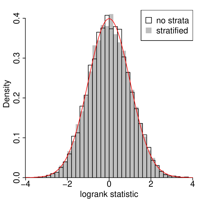
case i

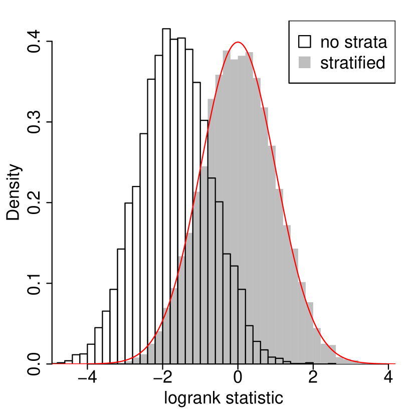
case ii

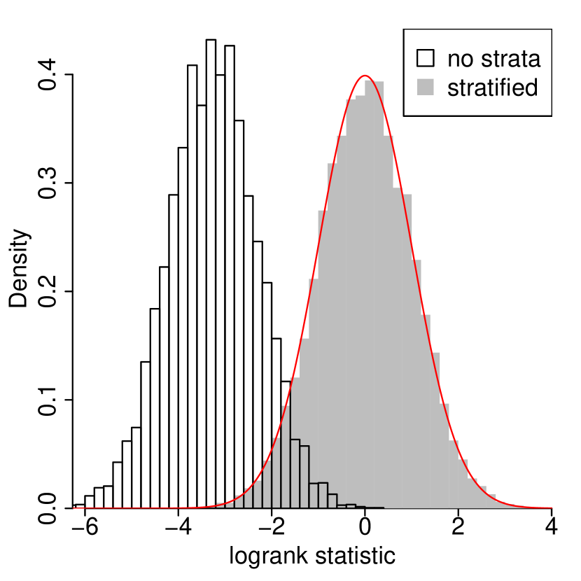
case iii

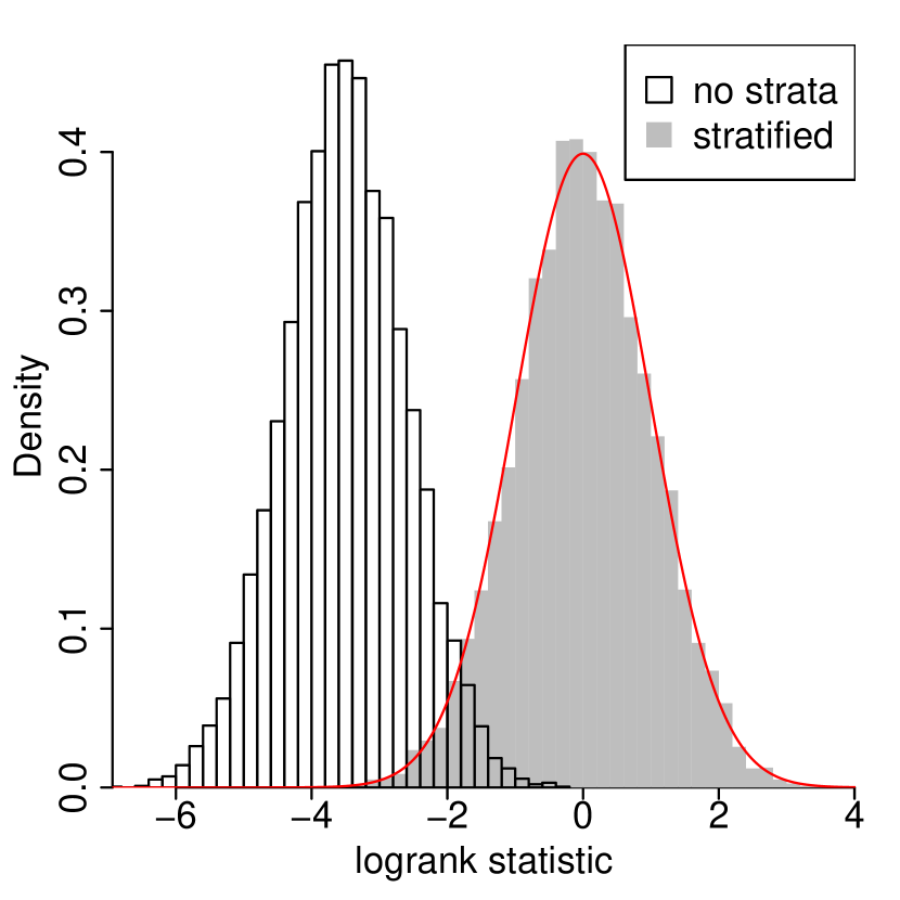
case iv

Figure 2: Histograms of the logrank and stratified logrank statistics under homogeneous/heterogeneous treatment assignment and censoring mechanisms as in Table 4. The white histograms denote the distributions of the logrank statistic, and the gray histograms denote the distributions of the stratified logrank statistic. The red lines denote the density of a standard Gaussian distribution.

First, we study the distribution of the logrank statistic under the four cases in Table 4 for generating the treatment assignments and potential censoring times. To mimic finite population inference, we simulate the fixed potential event times as in (4.5), and the resulting distribution for the logrank statistic will be its conditional distribution given $(\bm{T}(1),\bm{T}(0))$ fixed at (4.5). The white histograms in Figure 2 show the distributions of the logrank statistic under the four cases with or without heterogeneity in the treatment assignment or censoring mechanisms. From Figure 2, when there exists heterogeneity in treatment assignment or censoring mechanisms, i.e., Assumptions 1 or 2 fail, the logrank statistic is no longer close to be standard Gaussian distributed. We also conduct simulations with random potential event times from (4.1), and the corresponding histograms under the four cases are similar to that with fixed potential event times, as shown in Figure A4 in the Supplementary Material. In simple words, even with randomly generated potential event times, heterogeneity in the treatment assignment or censoring mechanisms still invalidates the logrank test.

Second, we study the distribution of the stratified logrank test under the previous simulation setting, where the stratified logrank statistic will be introduced and discussed shortly in the next section. In particular, we stratify on the covariates $X_{i}$’s in (4.1). The gray histograms in Figure 2 show the distributions of the stratified logrank statistic under the four cases in Table 4. From Figure 2, they are all close to a standard Gaussian distribution, indicating that the stratified logrank test is approximately valid. This phenomena is also true when the potential event times are randomly generated, as shown in Figure A4 in the Supplementary Material. Comparing the white and gray histograms in Figure 2, stratifying on the covariates $X_{i}$’s is crucial to ensure the validity of the logrank test. Intuitively, this is because, within each stratum defined by the covariates $X_{i}$’s, both the treatment assignment and censoring mechanisms become homogeneous across units. In the next section, we will give a more detailed discussion for the stratified logrank test, and provide rigorous conditions to ensure its asymptotic validity.

Extension to Stratified Logrank Test

We provide a solution to possible violation of Assumptions 1 or 2, namely the stratified logrank test (Mantel and Haenszel 1959), under the scenario where a categorical pretreatment covariate can fully adjust the inhomogeneity of treatment assignment and censoring mechanisms across units.

In usual superpopulation inference, the stratified logrank test is invoked when we want to adjust for some covariates that may be related to or can help explain heterogeneity in the event times. In finite population inference with i.i.d. treatment assignment and censoring (i.e., Assumptions 1 and 2 hold), as discussed in Sections 5 and 6, the potential event times are allowed to be any constants and can thus have arbitrary heterogeneity across units. Therefore, we are able to conduct valid inference using the original logrank test even if we ignore some covariates related to the event times. However, as demonstrated by simulation in Section 7, the stratified logrank test can still be useful in finite population inference if the distributions of treatment assignment and potential censoring times depend on some pretreatment covariates. For example, the treatment assignment may come from a randomized block design with varying probabilities of receiving active treatment across blocks as in (7.1), and the censoring pattern may differ across units with different covariates as in (7.2).

Below we first introduce the stratified logrank statistic. Suppose that the units are divided into $S$ strata. For units in each stratum $s\in\{1,2,\ldots,S\}$, similar to Section 5.2, let $L_{[s]}$ be the overall observed-expected difference, and $U_{[s]}$ be the corresponding overall variance. We can then represent the (standardized) stratified logrank statistic as

$$\text{SLR}\equiv\left(\sum_{s=1}^{S}U_{[s]}\right)^{-1/2}\cdot\sum_{s=1}^{S}L_{[s]}.$$ (8.1)

When the treatment assignments and potential censoring times are independent across strata, and Assumptions 1 and 2 hold within each stratum, the observed-expected differences $L_{[s]}$’s, as well as the variances $U_{[s]}$’s, are mutually independent for all $1\leq s\leq S$, and the means and variances for the randomization distributions of the $L_{[s]}$’s can be similarly derived as in Theorem 3. These immediately imply the first two moments of the randomization distribution of the total observed-expected difference $\sum_{s=1}^{S}L_{[s]}$. Specifically, conditioning on all the potential event times, $\sum_{s=1}^{S}L_{[s]}$ has mean zero, and $\sum_{s=1}^{S}U_{[s]}$ is an unbiased variance estimator for it. Therefore, SLR is essentially a standardization of the total observed-expected difference. To establish the asymptotic Gaussianity of the stratified logrank statistic, we introduce the following regularity condition.

Condition 3.

Along the sequence of finite populations satisfying $H_{0}$ in (2.1), as $n\rightarrow\infty$, the number of strata $S$ is fixed, and for each stratum $1\leq s\leq S$,

• the number of units in stratum $s$ goes to infinity,

• Condition 1 or 2 holds for units within stratum $s$.

In Condition 3, the number of units within each stratum increases with the total sample size $n$, but the proportion of units within each stratum does not need to have a limit. From the discussion for Conditions 1 and 2 in Section 6, when units within each stratum are i.i.d. samples from some superpopulation, some weak conditions on the superpopulation can ensure that Condition 3 holds with probability one. The following theorem shows that Condition 3 is sufficient for the asymptotic standard Gaussianity of the stratified logrank statistic SLR.

Theorem 6.

Under the null hypothesis $H_{0}$ in (2.1) and conditioning on all the potential event times, if (a) the treatment assignments and potential censoring times, $(Z_{i},C_{i}(1),C_{i}(0))$’s, are mutually independent across all units, (b) Assumptions 1 and 2 hold within each stratum, and (c) Condition 3 holds, then the stratified logrank statistic (8.1) is asymptotically standard Gaussian, i.e.,

$$\text{SLR}\mid\bm{T}(1),\bm{T}(0)\stackrel{{\scriptstyle d}}{{\longrightarrow}}\mathcal{N}(0,1).$$

In Theorem 6, we only require Assumptions 1 and 2 to hold within each stratum, and thus allow the probability of receiving the active treatment and the joint distribution of the potential censoring times under treatment and control to vary across strata. Thus, Theorem 6 is particularly useful for randomized block designs and when the censoring mechanism varies across strata, as demonstrated by simulation in Section 7. Moreover, similar to the discussion at the end of Section 2.2, we can relax condition (b) in Theorem 6 by instead requiring $(Z_{i},C_{i}(1),C_{i}(0))$’s to be independent of the potential event times and i.i.d. within each stratum, allowing dependence between the treatment assignment and the potential censoring times.

The choice of strata is an important issue in practice. To ensure the validity of the stratified logrank test, we need to consider the covariates that affect either the treatment assignment or potential censoring times. However, the stratified logrank test can only take into account discrete covariates. It will be interesting to extend the randomization-based logrank test to adjust for more general (continuous) covariates, possibly utilizing ideas from inverse probability weighting (Horvitz and Thompson 1952; Rosenbaum and Rubin 1983; Hernán and Robins 2020), Cox regression models (Cox 1972) and regression adjustment for randomized experiments without censoring (Lin 2013; Guo and Basse 2021).

Conclusion and Discussion

We studied the randomization distribution of the logrank statistic when the treatment assignment and potential censoring times are i.i.d. across all units, and proved its asymptotic standard Gaussianity under certain regularity conditions. The theory developed here does not require any distributional assumption on the potential event times. It supplements the classical theory under usual superpopulation inference, and helps provide a broader justification for the logrank test. We invoked the stratified logrank test to overcome the inhomogeneity in treatment assignment and censoring mechanisms among units, and studied its randomization distribution as well as the corresponding asymptotic approximation.

In this paper we focus mainly on the logrank test. It will be interesting to extend the discussion to other variants or generalizations of the logrank test. For example, researchers have considered weighted logrank tests (see, e.g., Fleming and Harrington 1991), and recently Fernández et al. (2021) considered a kernel logrank test, where the test statistic corresponds to the supremum of a potentially infinite collection of weighted logrank statistics with weighting functions belonging to a reproducing kernel Hilbert space.

Supplementary Material

Appendix A1 discusses the relaxation of Assumptions 1 and 2, by allowing dependence between the treatment assignment and potential censoring times.

Appendix A2 summarizes and compares justifications for the logrank test from both superpopulation and finite population inferences.

Appendix A3 provides additional simulation results for the main text.

Appendix A4 provides the proofs for the exact randomization distribution of the logrank statistic.

Appendix A5 provides the proof for the asymptotic standard Gaussianity of the logrank statistic when the number of potentially distinct event times goes to infinity as the sample size goes to infinity.

Appendix A6 provides the proof for the asymptotic standard Gaussianity of the logrank statistic when the number of potentially distinct event times is bounded as the sample size increases.

Appendix A7 provides the proof for the asymptotic standard Gaussianity of the stratified logrank statistic.

Throughout the proofs of all lemmas and theorems from Appendix A4–A7, we are all conducting finite population inference by conditioning on all the potential event times $\bm{T}(1)$ and $\bm{T}(0)$. For clarification, in the statement of the lemmas, we write such conditioning on $(\bm{T}(1),\bm{T}(0))$ explicitly. For descriptive convenience, in the proofs of the lemmas and the theorems, we suppress the conditioning on $(\bm{T}(1),\bm{T}(0))$, assume the potential event times are always conditioned on implicitly, and thus equivalently view the $T_{i}(1)$’s and $T_{i}(0)$’s as fixed constants.

Relaxation of Assumptions 1 and 2

If we relax the independence between the treatment assignment and potential censoring times as in Assumptions 1 and 2, the results on finite population inference in Sections 5 and 6 still hold except for a slight modification on the definition of $G_{z}(\cdot)$ for $z=0,1$. Specifically, we can replace Assumptions 1 and 2 by the following assumption on both the treatment assignment and censoring mechanisms.

Assumption A1.

The treatment assignments and potential censoring times are independent of the potential event times, in the sense that $(\bm{Z},\bm{C}(1),\bm{C}(0))$ $\begin{picture}(9.0,8.0)\put(0.0,0.0){\line(1,0){9.0}} \put(3.0,0.0){\line(0,1){8.0}} \put(6.0,0.0){\line(0,1){8.0}} \end{picture}(\bm{T}(1),\bm{T}(0))$, and the $(Z_{i},C_{i}(1),C_{i}(0))$’s are i.i.d. across all units.

Assumption A1 is more general than Assumptions 1 and 2. It allows the treatment assignment to depend on the potential censoring times. For the randomization distribution of the logrank statistic, all the conclusions established under Assumptions 1 and 2 also hold under Assumption A1, with the survival functions $G_{z}(\cdot)$’s changed to $\overline{G}_{z}(\cdot)$’s, where $\overline{G}_{z}(c)\equiv\text{pr}(C_{i}(z)\geq c\mid Z_{i}=z)$ for any $c\in\mathbb{R}$ and $z=0,1$.

Below we explain why the theory developed in Sections 5 and 6 is still true when Assumption A1 holds instead of Assumptions 1 and 2. For each unit $i$, we introduce two independent random variables $\overline{C}_{i}(1)$ and $\overline{C}_{i}(0)$ for a pair of pseudo potential censoring times that follow the distributions of $C_{i}(1)$ given $Z_{i}=1$ and $C_{i}(0)$ given $Z_{i}=0$, respectively, i.e.,

$$\overline{C}_{i}(1)\sim C_{i}(1)\mid Z_{i}=1,\quad\overline{C}_{i}(0)\sim C_{i}(0)\mid Z_{i}=0,\quad\overline{C}_{i}(1)\begin{picture}(9.0,8.0)\put(0.0,0.0){\line(1,0){9.0}} \put(3.0,0.0){\line(0,1){8.0}} \put(6.0,0.0){\line(0,1){8.0}} \end{picture}\overline{C}_{i}(0).$$

We further assume the pseudo potential censoring times $(\overline{C}_{i}(1),\overline{C}_{i}(0))$’s are i.i.d.  across all units, and they are independent of the treatment assignments $Z_{i}$’s. By construction, if the units’ potential censoring times were replaced by the pseudo potential censoring times $(\overline{C}_{i}(1),\overline{C}_{i}(0))$’s, Assumptions 1 and 2 would hold and all the results established in Sections 5 and 6, including the central limit theorems for the logrank statistics, would be true. Note that, by construction, for each unit $i$, conditional on $Z_{i}$, the realized pseudo censoring time $\overline{C}_{i}\equiv Z_{i}\overline{C}_{i}(1)+(1-Z_{i})\overline{C}_{i}(0)$ follows the same distribution as the realized censoring time $C_{i}$, and consequently,

$$(\overline{C}_{1},\overline{C}_{2},\ldots,\overline{C}_{n})\mid\bm{Z}\ \sim\ (C_{1},C_{2},\ldots,C_{n})\mid\bm{Z}.$$

This implies that, under Assumption A1 and conditioning on all the potential event times, the logrank statistic with the original potential censoring times $(C_{i}(1),C_{i}(0))$’s follows the same distribution as that with the pseudo potential censoring times $(\overline{C}_{i}(1),\overline{C}_{i}(0))$’s. Therefore, for the randomization distribution of the logrank statistic, all the conclusions established under Assumptions 1 and 2 also hold under Assumption A1, with the survival functions $G_{z}(\cdot)$’s for the potential censoring times changed to survival functions $\overline{G}_{z}(\cdot)$’s for the pseudo potential censoring times. Specifically, $\overline{G}_{z}(c)\equiv\text{pr}(\overline{C}_{i}(z)\geq c)=\text{pr}(C_{i}(z)\geq c\mid Z_{i}=z)$, for any $c\in\mathbb{R}$ and $z=0,1$.

Summary: broader justifications for the logrank test

From the discussion in Sections 3–6 and Appendix A1, finite population inference can provide additional justification for the validity of the logrank test, relaxing the distributional assumptions on the potential event times and supplementing the classical theory from usual superpopulation inference. Below we summarize justifications for the logrank test from both the superpopulation inference [see Gill, 1980, Fleming and Harrington, 1991] and finite population inference (see Sections 5 and 6 and Appendix A1). We assume that the treatment assignments and potential censoring times are independent of the potential event times, i.e., $(\bm{Z},\bm{C}(1),\bm{C}(0))\begin{picture}(9.0,8.0)\put(0.0,0.0){\line(1,0){9.0}} \put(3.0,0.0){\line(0,1){8.0}} \put(6.0,0.0){\line(0,1){8.0}} \end{picture}(\bm{T}(1),\bm{T}(0)).$ This assumption requires unconfounded treatment assignment and non-informative censoring, and is required for both the superpopulation and finite population inferences for the logrank test. Below we discuss additional assumptions needed for the superpopulation and finite population justifications, respectively.

First, conditional on the treatment assignment vector $\bm{Z}$ and all the potential censoring times $\bm{C}(1)$ and $\bm{C}(0)$, the realized event times $T_{i}$’s and censoring times $C_{i}$’s follow the general random censorship model with fixed censorship [Gill, 1980, Page 55]. From Gill [1980] and Fleming and Harrington [1991], if the potential event times $(T_{i}(1),T_{i}(0))$’s are i.i.d. across all units and the potential event times under treatment and control are identically distributed, i.e., $T_{i}(1)\sim T_{i}(0)$, then, with certain regularity conditions, the conditional distribution of the logrank statistic given $(\bm{Z},\bm{C}(1),\bm{C}(0))$ is asymptotically standard Gaussian. Therefore, the superpopulation inference can justify the logrank test without any distributional assumption on the treatment assignments and potential censoring times, and it relies crucially on the randomness in the i.i.d. sampling of units from a superpopulation. Second, from the discussion in Sections 5 and 6 and Appendix A1, if the treatment assignment and potential censoring times $(Z_{i},C_{i}(1),C_{i}(0))$’s are i.i.d. across all units, then, with certain regularity conditions (e.g., Condition 1 or 2), the conditional distribution of the logrank statistic given $(\bm{T}(1),\bm{T}(0))$ is asymptotically standard Gaussian under Fisher’s null $H_{0}$ in (2.1). Therefore, finite population inference can justify the logrank test without any distributional assumption on the potential event times, and it relies crucially on the randomness in the treatment assignments and censoring times. The top half of Table A1 summarizes the assumptions needed for the validity of the logrank test, with justifications from either superpopulation or finite population inference. From Table A1, finite population inference provide additional justification for the logrank test, supplementing the results from the classical superpopulation inference. Combining both types of inference, they provide a broader justification for the logrank test.

Table A1: Justifications for the asymptotic standard Gaussianity of logrank statistic. The potential event times are assumed to be independent of the treatment assignment and potential censoring times, i.e., $(\bm{T}(1),\bm{T}(0))\mathchoice{\mathrel{\hbox to0.0pt{$\displaystyle\perp$\hss}\mkern 2.0mu{\displaystyle\perp}}}{\mathrel{\hbox to0.0pt{$\textstyle\perp$\hss}\mkern 2.0mu{\textstyle\perp}}}{\mathrel{\hbox to0.0pt{$\scriptstyle\perp$\hss}\mkern 2.0mu{\scriptstyle\perp}}}{\mathrel{\hbox to0.0pt{$\scriptscriptstyle\perp$\hss}\mkern 2.0mu{\scriptscriptstyle\perp}}}(\bm{Z},\bm{C}(1),\bm{C}(0)).$ NDA stands for no distributional assumption. The top two rows considers the justification for the logrank test in general case. The bottom two rows considers the justification for the logrank test in a special case for testing Fisher’s null of no treatment effect on any unit under a Bernoulli randomized experiment.

	Potential event times	Treatment assignment &	Justification for
		censoring mechanisms	logrank test
	$(\bm{T}(1),\bm{T}(0))$	$(\bm{Z},\bm{C}(1),\bm{C}(0))$
General case	$(T_{i}(1),T_{i}(0))$’s are i.i.d., $T_{i}(1)\sim T_{i}(0)$	NDA	superpopulation
	$T_{i}(1)=T_{i}(0)$ for all $i$, NDA	$(Z_{i},C_{i}(1),C_{i}(0))$’s are i.i.d.	finite population
Special case	$T_{i}(1)=T_{i}(0)$’s are i.i.d.	NDA	superpopulation
	NDA	$(C_{i}(1),C_{i}(0))$’s are i.i.d.	finite population

Below we consider a special case in which we want to test Fisher’s null $H_{0}$ in (2.1) under a Bernoulli randomized experiment, i.e., Assumption 1 holds. Note that here Assumption 1 is justified by the physical randomization of the treatment assignment and it holds by the design of the experiment. In this special case, with certain regularity conditions, the logrank test is asymptotically valid when either the potential event times or potential censoring times are i.i.d. from a certain distribution, with justification from the superpopulation and finite population inferences, respectively. The bottom half of Table A1 summarizes the assumptions needed for the validity of the logrank test for testing Fisher’s null under a Bernoulli randomized experiment. From Table A1, we can see that the logrank test has a double-robust property, in the sense that it is asymptotically valid when either the potential event times or the potential censoring times are i.i.d. However, these two i.i.d. assumptions on potential event and censoring times, although they look symmetric, are quite different in nature. Specifically, the potential event times are of interest, while the potential censoring times are generally not of interest and introduce difficulties in inference for potential event times.

The appropriateness of the two i.i.d. assumptions can vary on a case-by-case basis. For potential event times it depends on whether the enrolled experimental units are homogeneous in their reactions to the treatment and control; it can be more reasonable when the enrolled units are randomly selected from some population of interest. For potential censoring times it depends on the censoring mechanism; in some cases, the experimenters are able to control the censoring mechanism and can thus make the assumption hold by homogeneous censoring for units under each treatment arm. For example, the experimenters can follow the units within the same treatment arm for random amounts of time drawn i.i.d. from some distribution, or even the same fixed amount of time. Also, in the case of administrative censoring in which units within the same treatment group are censored at the same time, the i.i.d. assumption on potential censoring times can hold if the time for entering the study is i.i.d. across all units.

As demonstrated by simulation in Section 7, under finite population inference, the logrank test can be invalid when the potential censoring times are not i.i.d. This indicates that, under finite population inference without any distributional assumption on the potential event times, the assumption of i.i.d. potential censoring times is in some way necessary for the validity of the logrank test; see also the discussion in Section 2.2.

More simulation results

In this section, we provide additional simulation results for the two sample $t$-test, the logrank test and the stratified logrank test in Sections 2.4, 4 and 7, respectively.

A3.1 A simulation study for the $t$-test under both superpopulation and finite population inferences

In this subsection, we conduct a simulation study for the $t$-test from both the superpopulation and finite population perspective, in parallel with Section 4. We assume the potential event times $\bm{T}(1)$ and $\bm{T}(0)$ are generated from (4.1), the treatment assignments are from a completely randomized experiment with half of the units receiving treatment and control, and all the potential censoring times are infinity, i.e., there is no censoring. Furthermore, the potential event times and the treatment assignments are mutually independent.

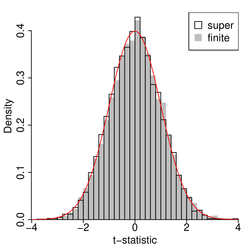
case 1

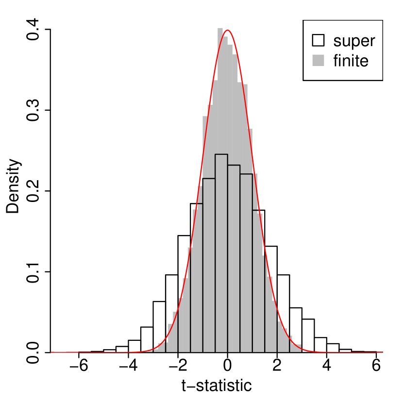
case 2

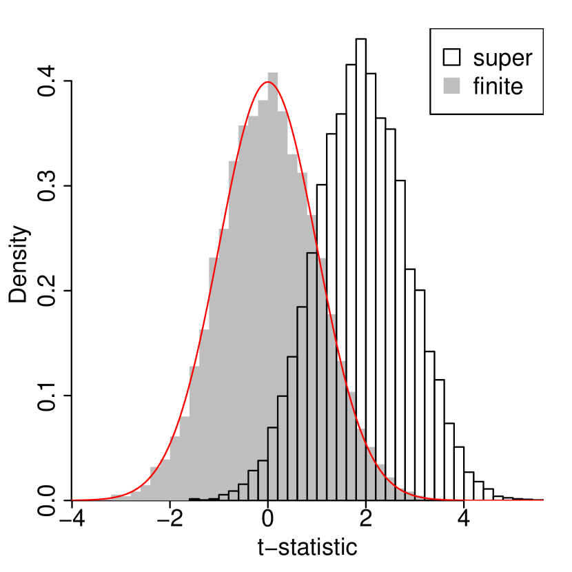
case 3

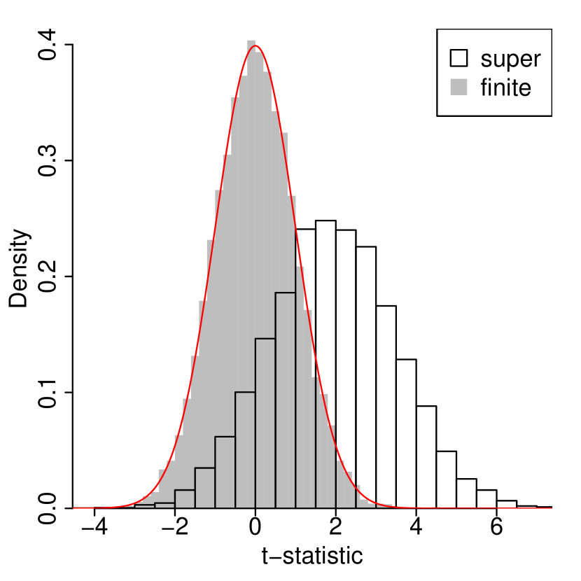
case 4

Figure A1: Histograms of the $t$-statistic in the superpopulation and finite population settings with parameters values in the four cases of Table 3. The white histograms denote the distributions of the $t$-statistic under superpopulation setting with random potential event times and fixed treatment assignments, and the gray histograms denote the distributions of the $t$-statistic under finite population setting with fixed potential event times and random treatment assignments. The red lines denote the density of a standard Gaussian distribution.

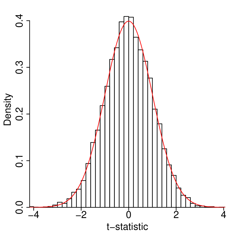
case 1

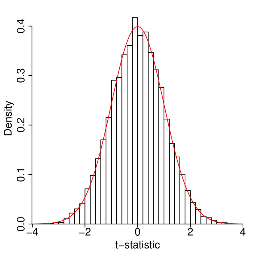
case 2

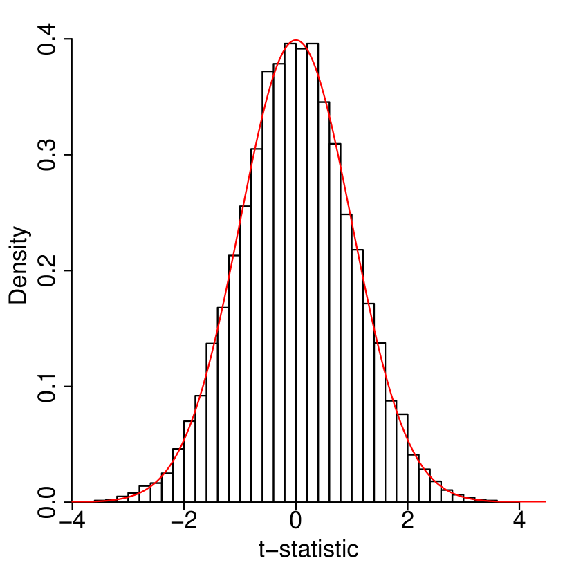
case 3

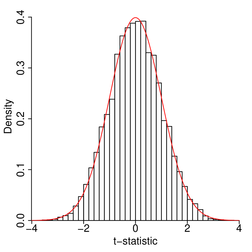
case 4

Figure A2: Histograms of the $t$-statistic when both the potential outcomes and treatment assignment are randomly and independently generated from (4.1) and (4.3), with parameters values in the four cases of Table 3. The red lines denote the density of a standard Gaussian distribution.

First, we mimic superpopulation inference where the treatment assignment $\bm{Z}$ is being conditioned on. We fix the treatment assignment $\bm{Z}$ as in (4.4), and generate the random potential event times $\bm{T}(1)$ and $\bm{T}(0)$ from model (4.1). The resulting distribution of the $t$-statistic is then the conditional distribution of $\mathfrak{T}$ given the treatment assignment $\bm{Z}$ in (4.4). In Figure A1, the four white histograms show the distributions of the $t$-statistic under the four cases in Table 3. From Figure A1, when there exist dependence or heterogeneity among the units’ potential event times, the conditional distribution of the $t$-statistic $\mathfrak{T}$ given $\bm{Z}$ in (4.4) is no larger close to a standard Gaussian distribution.

Second, we mimic finite population inference where the potential event times are being conditioned on. We fix the potential event times $\bm{T}(1)$ and $\bm{T}(0)$ as in (4.5), and generate the random treatment assignment $\bm{Z}$ from the completely randomized experiment. The resulting distribution of the $t$-statistic is then the conditional distribution of $\mathfrak{T}$ given the potential event times $\bm{T}(1)=\bm{T}(0)$ in (4.5). In Figure A1, the four gray histograms show the distributions of the $t$-statistic under the four cases in Table 3. From Figure A1, under all cases in Table 3 for generating the fixed potential event times in (4.5), the distributions of the $t$-statistic are all approximately standard Gaussian.

Third, we consider the setting where both the potential event times and the treatment assignment are random. Specifically, we generate the potential event times from model (4.1) and the treatment assignment from the completely randomized experiment, and they are mutually independent. Note that the distribution of the $t$-statistic here can be viewed as the conditional distribution of $\mathfrak{T}$ given $\bm{T}(1)$ and $\bm{T}(0)$ marginal over all potential event times. From the finite population simulation results, it is not surprising that the distributions of the $t$-statistic under all cases in Table 3 are close to a standard Gaussian distribution, as shown in Figure A2. Therefore, randomization justifies the usual two-sample $t$-test, and it does not require any distributional assumption on the potential event times.

A3.2 Additional simulation results for the logrank test

case 1

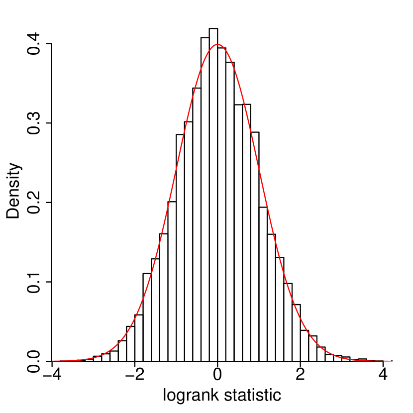
case 2

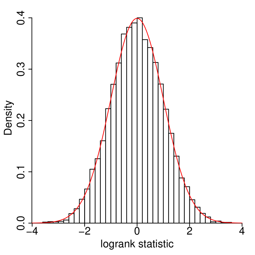
case 3

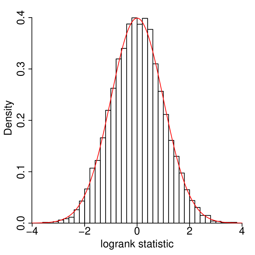
case 4

Figure A3: Histograms of the logrank statistic when the potential event times, potential censoring times and treatment assignment are mutually independent and randomly generated from (4.1), (4.2) and (4.3), respectively, with parameters values in the four cases of Table 3. The red lines denote the density of a standard Gaussian distribution.

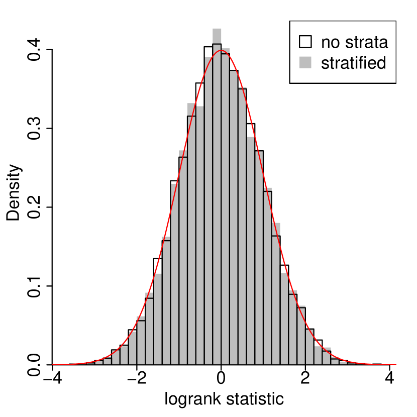
case i

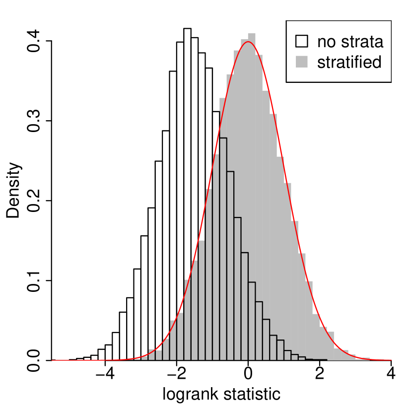
case ii

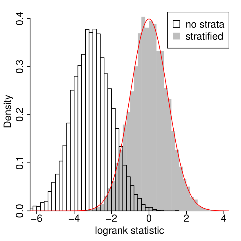
case iii

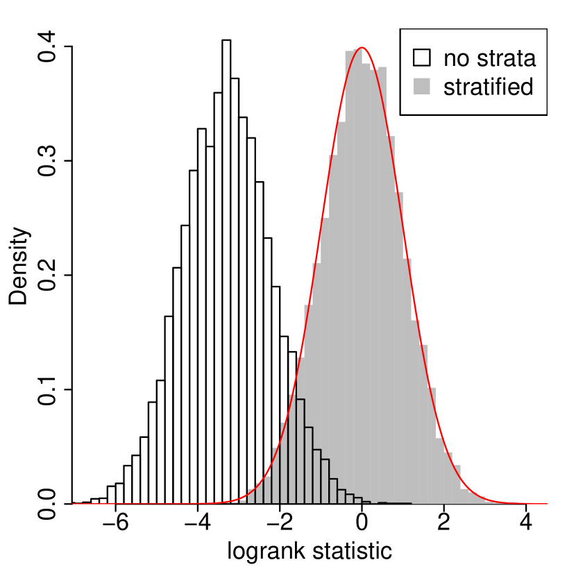
case iv

Figure A4: Histograms of the logrank and stratified logrank statistics under homogeneous/heterogeneous treatment assignment and censoring mechanisms as in Table 4, with mutually independent potential event times, potential censoring times and treatment assignment randomly generated from (4.1), (7.2) and (7.1), respectively. The white histograms denote the distributions of the logrank statistic, and the gray histograms denote the distributions of the stratified logrank statistic. The red lines denote the density of the standard Gaussian distribution.

Figure A3 shows the histograms of the logrank statistic, when the potential event times $(\bm{T}(1),\bm{T}(0))$, potential censoring times $(\bm{C}(1),\bm{C}(0))$ and treatment assignment $\bm{Z}$ are mutually independent and randomly generated from (4.1), (4.2) and (4.3), respectively. The parameters values for $\rho$ and $\theta$ are chosen as in the four cases in Table 3. From Figure A3, the distributions of the logrank statistic under all four cases are close to the standard Gaussian distribution. This is not surprising because we can view the distribution of the logrank statistic with random potential event times and random treatment assignment as the marginalization of the randomization distribution in (6.4), whose asymptotic standard Gaussianity is established in Section 6 and is also demonstrated in Figure 1.

Figure A4 shows the histograms of the original logrank statistic and the stratified logrank statistic based on the covariates $\bm{X}$ in (4.1), when the potential event times $(\bm{T}(1),\bm{T}(0))$, potential censoring times $(\bm{C}(1),\bm{C}(0))$ and treatment assignment $\bm{Z}$ are mutually independent and randomly generated from (4.1) with $\rho=0.5$ and $\theta=1$, (7.2) and (7.1), respectively. The values for $I_{z}$ and $I_{c}$ are chosen as in the four cases in Table 4. From Figure A4, the distribution of the logrank statistic is far from the standard Gaussian distribution, when there exists heterogeneity among units’ treatment assignment or censoring mechanisms. This indicates that Assumptions 1 and 2 are in some way necessary for the asymptotic standard Gaussianity of the logrank statistic. However, the distributions of the stratified logrank statistic under all four cases are close to the standard Gaussian distribution. This is not surprising because we can view the distribution of the stratified logrank statistic with random potential event times and random treatment assignment as the marginalization of the randomization distribution in Theorem 6, whose asymptotic Gaussianity is established there and is also demonstrated in Figure 2.

Exact randomization distribution of the logrank statistic

A4.1 Lemmas

For any integer $m\geq 0$ and constant $p\in[0,1]$, a random variable with probability mass function $m!/\{j!(m-j)!\}\cdot p^{j}(1-p)^{m-j}$ for $0\leq j\leq m$ is said to follow a binomial distribution with parameters $(m,p)$, denoted as $\text{Bin}(m,p)$. The following two lemmas study the randomization distribution of the treatment indicators for units at risk at time $t$ given observed information up to time $t$, and plays an important role in proving Theorems 1 and 2.

Lemma A1.

Under Assumptions 1 and 2 and the null hypothesis $H_{0}$ in (2.1), and conditioning on all the potential event times $\bm{T}(1)$ and $\bm{T}(0)$,

$$\quad\ \mathbb{E}\left\{Z_{i}\mathbbm{1}(W_{i}\geq t)\mid\bm{T}(1),\bm{T}(0),\mathbbm{1}(W_{i}\geq t),\Delta_{i}\mathbbm{1}(W_{i}=t)\right\}$$

$$=\mathbb{E}\left\{Z_{i}\mathbbm{1}(W_{i}\geq t)\mid\bm{T}(1),\bm{T}(0),\mathbbm{1}(W_{i}\geq t)\right\}$$

$$=\mathbbm{1}(W_{i}\geq t)\phi(t).$$

Lemma A2.

Under Assumptions 1 and 2 and the null hypothesis $H_{0}$ in (2.1), and conditioning on all the potential event times $\bm{T}(1)$ and $\bm{T}(0)$, for any time $t\geq 0$,

$$\quad\ \text{pr}\left\{\overline{D}_{1}(t)=A,\overline{N}_{1}(t)=B\mid\bm{T}(1),\bm{T}(0),\Delta_{i}\mathbbm{1}(W_{i}=t),\mathbbm{1}(W_{i}\geq t),1\leq i\leq n\right\}$$

$$=\binom{\overline{D}(t)}{A}\binom{\overline{N}(t)-\overline{D}(t)}{B-A}\{\phi(t)\}^{B}\{1-\phi(t)\}^{\overline{N}(t)-B}.$$

The following three lemmas study the randomization distributions of the $(N_{k},D_{k},N_{1k})$’s, and play an important role in characterizing the variance of the overall observed-expected difference $L$ in (5.2).

Lemma A3.

Under Assumptions 1 and 2 and the null hypothesis $H_{0}$ in (2.1), and conditioning on all the potential event times $\bm{T}(1)$ and $\bm{T}(0)$, for $1\leq k\leq K$, conditional on $N_{k}$, $D_{k}$ and $N_{1k}$ are independent, i.e.,

$$N_{1k}\begin{picture}(9.0,8.0)\put(0.0,0.0){\line(1,0){9.0}} \put(3.0,0.0){\line(0,1){8.0}} \put(6.0,0.0){\line(0,1){8.0}} \end{picture}D_{k}\mid\bm{T}(1),\bm{T}(0),N_{k},$$

and they follow hypergeometric and binomial distributions, respectively:

$$D_{k}\mid\bm{T}(1),\bm{T}(0),N_{k} \sim\text{HGeom}(n_{k},d_{k},N_{k}),$$

$$N_{1k}\mid\bm{T}(1),\bm{T}(0),N_{k} \sim\text{Bin}(N_{k},\phi_{k}).$$

Lemma A4.

Under Assumptions 1 and 2 and the null hypothesis $H_{0}$ in (2.1), and conditioning on all the potential event times $\bm{T}(1)$ and $\bm{T}(0)$, for $1\leq k\leq K$, $N_{k}$, $D_{k}$ and $N_{1k}$ all follow binomial distributions:

$$D_{k}\mid\bm{T}(1),\bm{T}(0) \sim\text{Bin}(d_{k},g_{k}),\ \ N_{1k}\mid\bm{T}(1),\bm{T}(0)\sim\text{Bin}(n_{k},g_{k}\phi_{k}),$$

$$N_{k}\mid\bm{T}(1),\bm{T}(0) \sim\text{Bin}(n_{k},g_{k}).$$

Lemma A5.

Under Assumptions 1 and 2 and the null hypothesis $H_{0}$, and conditioning on all the potential event times $\bm{T}(1)$ and $\bm{T}(0)$,

$$\mathbb{E}\left\{D_{k}(N_{k}-D_{k})\mid\bm{T}(1),\bm{T}(0),N_{k}\right\} =N_{k}(N_{k}-1)h_{k}(1-h_{k})\frac{n_{k}}{n_{k}-1},$$ (A1)

$$\mathbb{E}\left\{N_{1k}(N_{k}-N_{1k})\mid\bm{T}(1),\bm{T}(0),N_{k}\right\} =N_{k}(N_{k}-1)\phi_{k}(1-\phi_{k}).$$ (A2)

A4.2 Proofs of the lemmas

Proof of Lemma A1.

Because $\Delta_{i}\mathbbm{1}(W_{i}=t)=\mathbbm{1}(W_{i}\geq t)\mathbbm{1}(T_{i}(0)=t)$, $\Delta_{i}\mathbbm{1}(W_{i}=t)$ is a constant given $\mathbbm{1}(W_{i}\geq t)$. This implies

$$\quad\ \mathbb{E}\left\{Z_{i}\mathbbm{1}(W_{i}\geq t)\mid\mathbbm{1}(W_{i}\geq t),\Delta_{i}\mathbbm{1}(W_{i}=t)\right\}$$ (A3)

$$=\mathbb{E}\left\{Z_{i}\mathbbm{1}(W_{i}\geq t)\mid\mathbbm{1}(W_{i}\geq t)\right\}=\mathbbm{1}(W_{i}\geq t)\mathbb{E}\left(Z_{i}\mid W_{i}\geq t\right)$$

$$=\mathbbm{1}(W_{i}\geq t)\frac{\text{pr}(Z_{i}=1,W_{i}\geq t)}{\sum_{z=0}^{1}\text{pr}(Z_{i}=z,W_{i}\geq t)}.$$

By definition, we can simplify (A3) as

$$\quad\ \mathbb{E}\left\{Z_{i}\mathbbm{1}(W_{i}\geq t)\mid\mathbbm{1}(W_{i}\geq t),\Delta_{i}\mathbbm{1}(W_{i}=t)\right\}$$ (A4)

$$=\mathbbm{1}(W_{i}\geq t)\frac{\text{pr}(Z_{i}=1,C_{i}(1)\geq t,T_{i}(1)\geq t)}{\sum_{z=0}^{1}\text{pr}(Z_{i}=z,C_{i}(z)\geq t,T_{i}(z)\geq t)}$$

$$=\mathbbm{1}(W_{i}\geq t)\frac{\mathbbm{1}(T_{i}(1)\geq t)p_{1}G_{1}(t)}{\mathbbm{1}(T_{i}(1)\geq t)p_{1}G_{1}(t)+\mathbbm{1}(T_{i}(0)\geq t)p_{0}G_{0}(t)}.$$

Because under the null hypothesis $H_{0}$, $W_{i}\geq t$ implies that $T_{i}(1)=T_{i}(0)\geq t$, we can further simplify (A4) as

$$\quad\ \mathbb{E}\left\{Z_{i}\mathbbm{1}(W_{i}\geq t)\mid\mathbbm{1}(W_{i}\geq t),\Delta_{i}\mathbbm{1}(W_{i}=t)\right\}$$

$$=\mathbbm{1}(W_{i}\geq t)\frac{p_{1}G_{1}(t)}{p_{1}G_{1}(t)+p_{0}G_{0}(t)}$$

$$=\mathbbm{1}(W_{i}\geq t)\phi(t).$$

Therefore, Lemma A1 holds. ∎

Proof of Lemma A2.

For any $t\geq 0$, let

$$\overline{\mathcal{I}}(t)=\{i:\Delta_{i}\mathbbm{1}(W_{i}=t)=1,1\leq i\leq n\}$$

be the set of units having events at time $t$,

$$\overline{\mathcal{J}}(t)=\{i:\mathbbm{1}(W_{i}\geq t)=1,\Delta_{i}\mathbbm{1}(W_{i}=t)=0,1\leq i\leq n\}$$

be the set of units at risk but not having events at time $t$, and $|\overline{\mathcal{I}}(t)|$ and $|\overline{\mathcal{J}}(t)|$ be the cardinalities of these two sets. For any $t\geq 0$, we define a $\sigma$-algebra $\mathcal{E}(t)$ as follows:

$$\mathcal{E}(t)=\sigma\left\{\Delta_{i}\mathbbm{1}(W_{i}=t),\mathbbm{1}(W_{i}\geq t),1\leq i\leq n\right\}.$$

By definition, the conditional distribution of $\overline{D}_{1}(t)$ and $\overline{N}_{1}(t)$ given $\mathcal{E}(t)$ has the following equivalent forms:

$$\quad\ \text{pr}\left\{\overline{D}_{1}(t)=A,\overline{N}_{1}(t)=B\mid\mathcal{E}(t)\right\}$$ (A5)

$$=\text{pr}\left\{\sum_{i=1}^{n}Z_{i}\Delta_{i}\mathbbm{1}(W_{i}=t)=A,\ \sum_{i=1}^{n}Z_{i}\mathbbm{1}(W_{i}\geq t)=B\mid\mathcal{E}(t)\right\}$$

$$=\text{pr}\left\{\sum_{i\in\overline{\mathcal{I}}(t)}Z_{i}=A,\sum_{i\in\overline{\mathcal{I}}(t)\cup\overline{\mathcal{J}}(t)}Z_{i}=B\mid\mathcal{E}(t)\right\}$$

$$=\text{pr}\left\{\sum_{i\in\overline{\mathcal{I}}(t)}Z_{i}=A,\sum_{i\in\overline{\mathcal{J}}(t)}Z_{i}=B-A\mid\mathcal{E}(t)\right\}.$$

Under Assumptions 1 and 2, $(Z_{i},W_{i},\Delta_{i})$’s are mutually independent for $1\leq i\leq n$. Thus, from Lemma A1, conditional on $\mathcal{E}(t)$, $\sum_{i\in\overline{\mathcal{I}}(t)}Z_{i}$ follows a binomial distribution with parameters $(|\overline{\mathcal{I}}(t)|,\phi(t))$, $\sum_{i\in\overline{\mathcal{J}}(t)}Z_{i}$ follows a binomial distribution with parameters $(|\overline{\mathcal{J}}(t)|,\phi(t))$, and they are independent. Therefore, the conditional distribution (A5) has the following equivalent forms:

$$\quad\ \text{pr}\left\{\overline{D}_{1}(t)=A,\overline{N}_{1}(t)=B\mid\mathcal{E}(t)\right\}$$

$$=\binom{|\overline{\mathcal{I}}(t)|}{A}\{\phi(t)\}^{A}\{1-\phi(t)\}^{|\overline{\mathcal{I}}(t)|-A}\binom{|\overline{\mathcal{J}}(t)|}{B-A}\{\phi(t)\}^{B-A}\{1-\phi(t)\}^{|\overline{\mathcal{J}}(t)|-(B-A)}$$

$$=\binom{|\overline{\mathcal{I}}(t)|}{A}\binom{|\overline{\mathcal{J}}(t)|}{B-A}\{\phi(t)\}^{B}\{1-\phi(t)\}^{|\overline{\mathcal{I}}(t)|+|\overline{\mathcal{J}}(t)|-B}.$$

By definition, $|\overline{\mathcal{I}}(t)|=\overline{D}(t)$, $|\overline{\mathcal{J}}(t)|=\overline{N}(t)-\overline{D}(t),$ and thus Lemma A2 holds. ∎

Proof of Lemma A3.

First, we derive the conditional distribution of $N_{1k}$ given $N_{k}$, and show that $N_{1k}$ and $D_{k}$ are conditionally independent given $N_{k}$. For any $1\leq k\leq K$, from Lemma A1 and the mutual independence of the $(Z_{i},W_{i},\Delta_{i})$’s under Assumptions 1 and 2, we can know that

$$\quad\ \sum_{i=1}^{n}Z_{i}\mathbbm{1}(W_{i}\geq t_{k})\mid\mathbbm{1}(W_{j}\geq t_{k}),\Delta_{j}\mathbbm{1}(W_{j}=t_{k}),1\leq j\leq n$$ (A6)

$$\sim\ \text{Bin}\left(N_{k},\phi_{k}\right).$$

By definition, both $N_{k}$ and $D_{k}$ are deterministic functions of the $\mathbbm{1}(W_{j}\geq t_{k})$’s and $\Delta_{j}\mathbbm{1}(W_{j}=t_{k})$’s, respectively. Thus, from (A6), conditional on $N_{k}$, $N_{1k}$ follows a binomial distribution with parameters $(N_{k},\phi_{k})$, and it is independent of $D_{k}$, i.e.,

$$N_{1k}\mid N_{k}\sim\text{Bin}(N_{k},\phi_{k}),\ \ \text{ and }\ \ N_{1k}\begin{picture}(9.0,8.0)\put(0.0,0.0){\line(1,0){9.0}} \put(3.0,0.0){\line(0,1){8.0}} \put(6.0,0.0){\line(0,1){8.0}} \end{picture}D_{k}\mid N_{k}.$$

Second, we study the distribution of $(D_{k},N_{k})$, and derive the conditional distribution of $D_{k}$ given $N_{k}$. Under $H_{0}$, for any unit $i$ with $\Delta_{i}\mathbbm{1}(W_{i}=t_{k})=1$, we must have $T_{i}(1)=T_{i}(0)=t_{k}$. Similarly, for any unit $i$ with $\mathbbm{1}(W_{i}\geq t_{k})=1$, we must have $T_{i}(1)=T_{i}(0)\geq t_{k}$. Thus, by definition, $D_{k}\leq d_{k}$ and $D_{k}\leq N_{k}\leq n_{k}$. For any constant nonnegative integers $A,B$ satisfying $A\leq d_{k}$ and $A\leq B\leq n_{k}$, the probability that $D_{k}=A$ and $N_{k}=B$ has the following equivalent forms:

$$\quad\ \text{pr}\left(D_{k}=A,N_{k}=B\right)$$ (A7)

$$=\text{pr}\left(\sum_{i=1}^{n}\Delta_{i}\mathbbm{1}(W_{i}=t_{k})=A,\ \sum_{i=1}^{n}\mathbbm{1}(W_{i}\geq t_{k})=B\right)$$

$$=\text{pr}\left(\sum_{i:T_{i}(0)=t_{k}}\Delta_{i}\mathbbm{1}(W_{i}=t_{k})=A,\sum_{i:T_{i}(0)\geq t_{k}}\mathbbm{1}(W_{i}\geq t_{k})=B\right).$$

Under $H_{0}$, for any unit $i$ with $T_{i}(0)=t_{k}$, we must have $\Delta_{i}\mathbbm{1}\{W_{i}=t_{k}\}=\mathbbm{1}\{W_{i}\geq t_{k}\}$. Thus, (A7) reduces to

$$\quad\ \text{pr}\left(D_{k}=A,N_{k}=B\right)$$ (A8)

$$=\text{pr}\left(\sum_{i:T_{i}(0)=t_{k}}\mathbbm{1}(W_{i}\geq t_{k})=A,\sum_{i:T_{i}(0)\geq t_{k}}\mathbbm{1}(W_{i}\geq t_{k})=B\right)$$

$$=\text{pr}\left(\sum_{i:T_{i}(0)=t_{k}}\mathbbm{1}(W_{i}\geq t_{k})=A,\sum_{i:T_{i}(0)>t_{k}}\mathbbm{1}(W_{i}\geq t_{k})=B-A\right).$$

Because (i) for any unit $i$ with $T_{i}(1)=T_{i}(0)\geq t_{k}$, $\text{pr}(W_{i}\geq t_{k})=\text{pr}\left(C_{i}\geq t_{k}\right)=G(t_{k})=g_{k},$ and (ii) $W_{i}$’s are mutually independent for $1\leq i\leq n$, we can know that

$$D_{k} =\sum_{i:T_{i}(0)=t_{k}}\mathbbm{1}(W_{i}\geq t_{k})\sim\text{Bin}(d_{k},g_{k}),$$ (A9)

$$N_{k}-D_{k} =\sum_{i:T_{i}(0)>t_{k}}\mathbbm{1}(W_{i}\geq t_{k})\sim\text{Bin}(n_{k}-d_{k},g_{k}),$$

and they are mutually independent. Thus, we can further simplify (A8) as

$$\quad\ \text{pr}\left(D_{k}=A,N_{k}=B\right)$$

$$=\binom{d_{k}}{A}g_{k}^{A}(1-g_{k})^{d_{k}-A}\binom{n_{k}-d_{k}}{B-A}g_{k}^{B-A}(1-g_{k})^{n_{k}-d_{k}-(B-A)}$$

$$=\binom{d_{k}}{A}\binom{n_{k}-d_{k}}{B-A}g_{k}^{B}(1-g_{k})^{n_{k}-B}.$$

This immediately implies the marginal distribution of $N_{k}$:

$$\quad\ \text{pr}\left(N_{k}=B\right)$$ (A10)

$$=\sum_{A}\text{pr}\left(D_{k}=A,N_{k}=B\right)=\sum_{A}\binom{d_{k}}{A}\binom{n_{k}-d_{k}}{B-A}g_{k}^{B}(1-g_{k})^{n_{k}-B}$$

$$=\binom{n_{k}}{B}g_{k}^{B}(1-g_{k})^{n_{k}-B},$$

i.e., $N_{k}$ follows a binomial distribution with parameters $(n_{k},g_{k})$. Therefore, the conditional distribution of $D_{k}$ given $N_{k}$ has the following equivalent forms:

$$\text{pr}\left(D_{k}=A\mid N_{k}=B\right) =\frac{\text{pr}(D_{k}=A,N_{k}=B)}{\text{pr}(N_{k}=B)}=\frac{\binom{d_{k}}{A}\binom{n_{k}-d_{k}}{B-A}g_{k}^{B}(1-g_{k})^{n_{k}-B}}{\binom{n_{k}}{B}g_{k}^{B}(1-g_{k})^{n_{k}-B}}$$

$$=\frac{\binom{d_{k}}{A}\binom{n_{k}-d_{k}}{B-A}}{\binom{n_{k}}{B}},$$

i.e., conditional on $N_{k}$, $D_{k}$ follows a hypergeometric distribution with parameters $(n_{k},d_{k},N_{k})$.

From the above, Lemma A3 holds. ∎

Proof of Lemma A4.

First, from (A9), $D_{k}$ follows a binomial distribution with parameters $(d_{k},g_{k})$. Second, from (A10), $N_{k}$ follows a binomial distribution with parameters $(n_{k},g_{k})$. Third, because (i) $N_{k}\sim\text{Bin}(n_{k},g_{k})$ and (ii) $N_{1k}\mid N_{k}\sim\text{Bin}(N_{k},\phi_{k})$ from Lemma A3, the property of binomial distributions implies that $N_{1k}\sim\text{Bin}(n_{k},g_{k}\phi_{k})$. From the above, Lemma A4 holds. ∎

Proof of Lemma A5.

First, we prove (A1). The left hand side of (A1) has the following equivalent forms:

$$\quad\ \mathbb{E}\left\{D_{k}(N_{k}-D_{k})\mid N_{k}\right\}$$ (A11)

$$=N_{k}\mathbb{E}\left(D_{k}\mid N_{k}\right)-\mathbb{E}\left(D_{k}^{2}\mid N_{k}\right)$$

$$=N_{k}\mathbb{E}\left(D_{k}\mid N_{k}\right)-\left\{\mathbb{E}\left(D_{k}\mid N_{k}\right)\right\}^{2}-\text{Var}\left(D_{k}\mid N_{k}\right)$$

$$=\left\{N_{k}-\mathbb{E}\left(D_{k}\mid N_{k}\right)\right\}\mathbb{E}\left(D_{k}\mid N_{k}\right)-\text{Var}\left(D_{k}\mid N_{k}\right).$$

From Lemma A3 and the property of hypergeometric distribution, we have

$$\mathbb{E}\left\{D_{k}(N_{k}-D_{k})\mid N_{k}\right\} =\left(N_{k}-N_{k}h_{k}\right)N_{k}h_{k}-\frac{d_{k}(n_{k}-d_{k})N_{k}(n_{k}-N_{k})}{n_{k}^{2}(n_{k}-1)}$$

$$=N_{k}^{2}(1-h_{k})h_{k}-N_{k}h_{k}(1-h_{k})\frac{n_{k}-N_{k}}{n_{k}-1}$$

$$=N_{k}(N_{k}-1)h_{k}(1-h_{k})\frac{n_{k}}{n_{k}-1}.$$

Second, we prove (A2). By the same logic as (A11),

$$\quad\ \mathbb{E}\left\{N_{1k}(N_{k}-N_{1k})\mid N_{k}\right\}$$ (A12)

$$=\left\{N_{k}-\mathbb{E}\left(N_{1k}\mid N_{k}\right)\right\}\mathbb{E}\left(N_{1k}\mid N_{k}\right)-\text{Var}\left(N_{1k}\mid N_{k}\right).$$

From Lemma A3 and the property of binomial distribution, we have

$$\mathbb{E}\left\{N_{1k}(N_{k}-N_{1k})\mid N_{k}\right\} =(N_{k}-N_{k}\phi_{k})N_{k}\phi_{k}-N_{k}\phi_{k}(1-\phi_{k})$$

$$=N_{k}^{2}(1-\phi_{k})\phi_{k}-N_{k}\phi_{k}(1-\phi_{k})$$

$$=N_{k}(N_{k}-1)\phi_{k}(1-\phi_{k}).$$

From the above, Lemma A5 holds. ∎

A4.3 Proofs of the theorems

Proof of Theorem 1.

From Lemma A2,

$$\ \quad\text{pr}\left\{\overline{N}_{1}(t)=B\mid\Delta_{i}\mathbbm{1}(W_{i}=t),\mathbbm{1}(W_{i}\geq t),1\leq i\leq n\right\}$$

$$=\sum_{A}\text{pr}\left\{\overline{D}_{1}(t)=A,\overline{N}_{1}(t)=B\mid\Delta_{i}\mathbbm{1}(W_{i}=t),\mathbbm{1}(W_{i}\geq t),1\leq i\leq n\right\}$$

$$=\sum_{A}\binom{\overline{D}(t)}{A}\binom{\overline{N}(t)-\overline{D}(t)}{B-A}\{\phi(t)\}^{B}\{1-\phi(t)\}^{\overline{N}(t)-B}$$

$$=\binom{\overline{N}(t)}{B}\{\phi(t)\}^{B}\{1-\phi(t)\}^{\overline{N}(t)-B},$$

and thus the conditional distribution of $\overline{D}_{1}(t)$ given $\overline{N}_{1}(t)$, $\Delta_{i}\mathbbm{1}(W_{i}=t)$’s, and $\mathbbm{1}(W_{i}\geq t)$’s is

$$\quad\ \text{pr}\left\{\overline{D}_{1}(t)=A\mid\overline{N}_{1}(t)=B,\Delta_{i}\mathbbm{1}(W_{i}=t),\mathbbm{1}(W_{i}\geq t),1\leq i\leq n\right\}$$ (A13)

$$=\frac{\text{pr}\left\{\overline{D}_{1}(t)=A,\overline{N}_{1}(t)=B\mid\Delta_{i}\mathbbm{1}(W_{i}=t),\mathbbm{1}(W_{i}\geq t),1\leq i\leq n\right\}}{\text{pr}\left\{\overline{N}_{1}(t)=B\mid\Delta_{i}\mathbbm{1}(W_{i}=t),\mathbbm{1}(W_{i}\geq t),1\leq i\leq n\right\}}$$

$$=\frac{\binom{\overline{D}(t)}{A}\binom{\overline{N}(t)-\overline{D}(t)}{B-A}\{\phi(t)\}^{B}\{1-\phi(t)\}^{\overline{N}(t)-B}}{\binom{\overline{N}(t)}{B}\{\phi(t)\}^{B}\{1-\phi(t)\}^{\overline{N}(t)-B}}$$

$$=\binom{\overline{D}(t)}{A}\binom{\overline{N}(t)-\overline{D}(t)}{B-A}/\binom{\overline{N}(t)}{B}.$$

From (A13), by the law of iterated expectation, we have

$$\quad\ \text{pr}\left\{\overline{D}_{1}(t)=A\mid\overline{N}_{1}(t),\overline{N}(t),\overline{D}(t)\right\}$$

$$=\mathbb{E}\left[\text{pr}\left\{\overline{D}_{1}(t)=A\mid\overline{N}_{1}(t),\Delta_{i}\mathbbm{1}(W_{i}=t),\mathbbm{1}(W_{i}\geq t),\forall i\right\}\mid\overline{N}_{1}(t),\overline{N}(t),\overline{D}(t)\right]$$

$$=\binom{\overline{D}(t)}{A}\binom{\overline{N}(t)-\overline{D}(t)}{\overline{N}_{1}(t)-A}/\binom{\overline{N}(t)}{\overline{N}_{1}(t)}.$$

Therefore, Theorem 1 holds. ∎

Proof of Theorem 2.

First, we show that conditional on $\mathcal{F}_{k-1}$, $D_{1k}$ follows a hypergeometric distribution with parameters $(N_{k},D_{k},N_{1k})$. For $1\leq k\leq K$, define a $\sigma$-algebra $\mathcal{H}_{k-1}$ as

$$\mathcal{H}_{k-1} =\sigma\left\{\mathbbm{1}(W_{i}\geq t_{q}),\Delta_{i}\mathbbm{1}(W_{i}=t_{q}),Z_{i}\Delta_{i}\mathbbm{1}(W_{i}=t_{q-1}),\vphantom{\sum_{j=1}^{n}Z_{j}\mathbbm{1}(t_{q}\leq W_{j}<t_{k})}\right.$$

$$\left.\qquad\qquad\qquad\qquad\qquad\sum_{j=1}^{n}Z_{j}\mathbbm{1}(t_{q}\leq W_{j}<t_{k}),\ 1\leq q\leq k,1\leq i\leq n\right\},$$

where $\mathbbm{1}(t_{k}\leq W_{j}<t_{k})$ is defined to be constant zero. The set of units having events at time $t_{k}$ is $\mathcal{I}_{k}=\{i:\Delta_{i}\mathbbm{1}(W_{i}=t_{k})=1,1\leq i\leq n\}$, and the set of units at risk but not having events at time $t_{k}$ is $\mathcal{J}_{k}=\{i:\mathbbm{1}(W_{i}\geq t_{k})=1,\Delta_{i}\mathbbm{1}(W_{i}=t_{k})=0,1\leq i\leq n\}.$ By definition, the cardinalities of sets $\mathcal{I}_{k}$ and $\mathcal{J}_{k}$ are $D_{k}$ and $N_{k}-D_{k}.$ We can then divide the information in $\mathcal{H}_{k-1}$ into three parts for disjoint sets of units: (i) $\mathcal{I}_{k}$, (ii) $\mathcal{J}_{k}$, and (iii)

$$\mathbbm{1}(W_{i}\geq t_{q}),\Delta_{i}\mathbbm{1}(W_{i}=t_{q}),Z_{i}\Delta_{i}\mathbbm{1}(W_{i}=t_{q-1}),\sum_{j\in\mathcal{I}_{k}^{c}\cap\mathcal{J}_{k}^{c}}Z_{j}\mathbbm{1}(t_{q}\leq W_{j}<t_{k}),$$

$$1\leq q\leq k,i\in\mathcal{I}_{k}^{c}\cap\mathcal{J}_{k}^{c}.$$

Under Assumptions 1 and 2, $(Z_{i},W_{i},\Delta_{i})$’s are mutually independent for $1\leq i\leq n$. Thus, the conditional distribution of $(D_{1k},N_{1k})$ given $\mathcal{H}_{K-1}$ has the following equivalent forms:

$$\quad\ \text{pr}\left(D_{1k}=A,N_{1k}=B\mid\mathcal{H}_{k-1}\right)$$ (A14)

$$=\text{pr}\left(D_{1k}=A,N_{1k}=B\mid\mathcal{I}_{k},\mathcal{J}_{k}\right)$$

$$=\text{pr}\left\{D_{1k}=A,N_{1k}=B\mid\Delta_{i}\mathbbm{1}(W_{i}=t_{k}),\mathbbm{1}(W_{i}\geq t_{k}),1\leq i\leq n\right\}.$$

From Lemma A2, we can further simplify (A14) as

$$\quad\ \text{pr}\left(D_{1k}=A,N_{1k}=B\mid\mathcal{H}_{k-1}\right)$$ (A15)

$$=\text{pr}\left\{\overline{D}_{1}(t_{k})=A,\overline{N}_{1}(t_{k})=B\mid\Delta_{i}\mathbbm{1}(W_{i}=t_{k}),\mathbbm{1}(W_{i}\geq t_{k}),\forall i\right\}$$

$$=\binom{D_{k}}{A}\binom{N_{k}-D_{k}}{B-A}\phi_{k}^{B}(1-\phi_{k})^{N_{k}-B}.$$

This implies that the marginal distribution of $N_{1k}$ given $\mathcal{H}_{k-1}$ is

$$\quad\ \text{pr}\left(N_{1k}=B\mid\mathcal{H}_{k-1}\right)$$ (A16)

$$=\sum_{A}\text{pr}\left(D_{1k}=A,N_{1k}=B\mid\mathcal{H}_{k-1}\right)$$

$$=\binom{N_{k}}{B}\phi_{k}^{B}(1-\phi_{k})^{N_{k}-B}.$$

From (A15) and (A16), the conditional distribution of $D_{1k}$ given $N_{1k}$ and $\mathcal{H}_{k-1}$ is

$$\text{pr}\left(D_{1k}=A\mid N_{1k},\mathcal{H}_{k-1}\right)=\frac{\binom{D_{k}}{A}\binom{N_{k}-D_{k}}{N_{1k}-A}}{\binom{N_{k}}{N_{1k}}}.$$

This implies that, conditional on $\mathcal{H}_{k-1}$ and $N_{1k}$, $D_{1k}$ follows a hypergeometric distribution with parameters $(N_{k},D_{k},N_{1k})$. Because for $1\leq q\leq k$,

$$\sum_{j=1}^{n}Z_{j}\mathbbm{1}(t_{q}\leq W_{j}<t_{k})+N_{1k} =\sum_{j=1}^{n}Z_{j}\mathbbm{1}(t_{q}\leq W_{j}<t_{k})+\sum_{j=1}^{n}Z_{j}\mathbbm{1}(W_{j}\geq t_{k})$$

$$=\sum_{j=1}^{n}Z_{j}\mathbbm{1}(W_{j}\geq t_{q}),$$

by definition, $(\mathcal{H}_{k-1},N_{1k})$ contains the same information as $\mathcal{F}_{k-1}$. Thus, the conditional distribution of $D_{1k}$ given $\mathcal{H}_{k-1}$ and $N_{1k}$ is the same as that given $\mathcal{F}_{k-1}$, i.e., conditional on $\mathcal{F}_{k-1}$, $D_{1k}$ follows a hypergeometric distribution with parameters $(N_{k},D_{k},N_{1k})$.

Second, we show that $\{D_{1k}-M_{k}\}_{k=1}^{K}$ is a martingale difference sequence with respect to filtration $\mathcal{F}_{k}$’s. By construction, $\mathcal{F}_{k}$’s constitute a filtration, and $D_{1k}$ is $\mathcal{F}_{k}$-measurable. From the first part, the property of hypergeometric distribution, and the definition of $M_{k}$, $\mathbb{E}(D_{1k}\mid\mathcal{F}_{k-1})=M_{k}$. Therefore, $\{D_{1k}-M_{k}\}_{k=1}^{K}$ is a martingale difference sequence with respect to filtration $\mathcal{F}_{k}$’s.

From the above, Theorem 2 holds. ∎

Proof of Theorem 3.

Theorem 2 immediately implies that $\mathbb{E}(L)=0$. From Lemmas A3 and A5,

$$\quad\ \mathbb{E}\left\{D_{k}(N_{k}-D_{k})N_{1k}(N_{k}-N_{1k})\mid N_{k}\right\}$$

$$=\mathbb{E}\left\{D_{k}(N_{k}-D_{k})\mid N_{k}\right\}\cdot\mathbb{E}\left\{N_{1k}(N_{k}-N_{1k})\mid N_{k}\right\}$$

$$=N_{k}^{2}(N_{k}-1)^{2}h_{k}(1-h_{k})\phi_{k}(1-\phi_{k})\frac{n_{k}}{n_{k}-1}.$$

This then implies

$$\mathbb{E}(V_{k}\mid N_{k}) =\mathbb{E}\left\{\frac{D_{k}(N_{k}-D_{k})N_{1k}(N_{k}-N_{1k})}{N_{k}^{2}(N_{k}-1)}\mid N_{k}\right\}$$

$$=\frac{N_{k}^{2}(N_{k}-1)^{2}h_{k}(1-h_{k})\phi_{k}(1-\phi_{k})}{N_{k}^{2}(N_{k}-1)}\frac{n_{k}}{n_{k}-1}$$

$$=(N_{k}-1+\mathbbm{1}\{N_{k}=0\})h_{k}(1-h_{k})\phi_{k}(1-\phi_{k})\frac{n_{k}}{n_{k}-1}.$$

From Lemma A4 and the law of iterated expectation, we have

$$\mathbb{E}(V_{k}) =\mathbb{E}\left\{\mathbb{E}(V_{k}\mid N_{k})\right\}$$ (A17)

$$=\left\{\mathbb{E}(N_{k})-1+\text{pr}(N_{k}=0)\right\}h_{k}(1-h_{k})\phi_{k}(1-\phi_{k})\frac{n_{k}}{n_{k}-1}$$

$$=\left\{n_{k}g_{k}-1+(1-g_{k})^{n_{k}}\right\}h_{k}(1-h_{k})\phi_{k}(1-\phi_{k})\frac{n_{k}}{n_{k}-1}$$

$$=\frac{n_{k}^{2}}{n_{k}-1}h_{k}(1-h_{k})\phi_{k}(1-\phi_{k})\left\{g_{k}-\frac{1-(1-g_{k})^{n_{k}}}{n_{k}}\right\}.$$

From Theorem 2 and the property of the martingale difference sequence,

$$\text{Var}(L) =\mathbb{E}(U)=\mathbb{E}\left(\sum_{k=1}^{K}V_{k}\right)=\sum_{k=1}^{K}\mathbb{E}(V_{k})$$

$$=\sum_{k=1}^{K}\frac{n_{k}^{2}}{n_{k}-1}h_{k}(1-h_{k})\phi_{k}(1-\phi_{k})\left\{g_{k}-\frac{1-(1-g_{k})^{n_{k}}}{n_{k}}\right\}.$$

Therefore, Theorem 3 holds. ∎

Asymptotic distribution of the logrank statistic with infinitely many distinct potential event times

A5.1 Lemmas

To prove Theorem 4, we need the following six lemmas. Lemma A6 gives a sufficient condition for the asymptotic Gaussianity of the logrank statistic using the martingale central limit theorem. It shows that the consistency of $U$ for the variance of $L$ is crucial for establishing the central limit theorem. To prove that conditioning on all the potential event times, $U/\mathbb{E}(U\mid\bm{T}(1),\bm{T}(0))\mid\bm{T}(1),\bm{T}(0)\stackrel{{\scriptstyle p}}{{\longrightarrow}}1$, or equivalently,

$$\frac{U-\mathbb{E}(U\mid\bm{T}(1),\bm{T}(0))}{\mathbb{E}(U\mid\bm{T}(1),\bm{T}(0))}\mid\bm{T}(1),\bm{T}(0)\stackrel{{\scriptstyle p}}{{\longrightarrow}}0,$$

we need to bound the denominator $\mathbb{E}(U\mid\bm{T}(1),\bm{T}(0))$ from below, and bound the absolute value of the numerator, $|U-\mathbb{E}(U\mid\bm{T}(1),\bm{T}(0))|,$ from above. Lemma A7 gives a lower bound of $\mathbb{E}(U\mid\bm{T}(1),\bm{T}(0))$. To bound $U-\mathbb{E}(U\mid\bm{T}(1),\bm{T}(0))$, for $1\leq k\leq K$, we decompose $V_{k}-\mathbb{E}(V_{k}\mid\bm{T}(1),\bm{T}(0))$ into four parts:

$$V_{k}-\mathbb{E}(V_{k}\mid\bm{T}(1),\bm{T}(0))=\xi_{1k}+\xi_{2k}+\xi_{3k}+\xi_{4k},$$

where

$$\xi_{1k} \equiv\frac{D_{k}(N_{k}-D_{k})}{N_{k}^{2}(N_{k}-1)}\left[N_{1k}(N_{k}-N_{1k})-\mathbb{E}\{N_{1k}(N_{k}-N_{1k})\mid\bm{T}(1),\bm{T}(0),N_{k}\}\right],$$

$$\xi_{2k} \equiv\frac{D_{k}\mathbb{E}\{N_{1k}(N_{k}-N_{1k})\mid\bm{T}(1),\bm{T}(0),N_{k}\}}{N_{k}^{2}(N_{k}-1)}$$

$$\quad\ \times\left\{(N_{k}-D_{k})-\mathbb{E}(N_{k}-D_{k}\mid\bm{T}(1),\bm{T}(0),N_{k})\right\},$$

$$\xi_{3k} \equiv\frac{D_{k}\mathbb{E}(N_{k}-D_{k}\mid\bm{T}(1),\bm{T}(0),N_{k})\mathbb{E}\{N_{1k}(N_{k}-N_{1k})\mid\bm{T}(1),\bm{T}(0),N_{k}\}}{N_{k}^{2}(N_{k}-1)}$$

$$\quad\ -\mathbb{E}(D_{k}\mid\bm{T}(1),\bm{T}(0))(1-h_{k})\phi_{k}(1-\phi_{k}),$$

$$\xi_{4k} \equiv\mathbb{E}(D_{k}\mid\bm{T}(1),\bm{T}(0))(1-h_{k})\phi_{k}(1-\phi_{k})-\mathbb{E}(V_{k}\mid\bm{T}(1),\bm{T}(0)).$$

Because $D_{K}=N_{K}$ by definition, we have $V_{K}=\mathbb{E}(V_{K})=0$, and

$$\quad\ U-\mathbb{E}(U\mid\bm{T}(1),\bm{T}(0))$$ (A1)

$$=\sum_{k=1}^{K-1}\left\{V_{k}-\mathbb{E}(V_{k}\mid\bm{T}(1),\bm{T}(0))\right\}$$

$$=\sum_{k=1}^{K-1}\xi_{1k}+\sum_{k=1}^{K-1}\xi_{2k}+\sum_{k=1}^{K-1}\xi_{3k}+\sum_{k=1}^{K-1}\xi_{4k}.$$

Lemmas A8–A11 give upper bounds for the four terms in (A1), separately. These further provide a probability upper bound for $U-\mathbb{E}(U\mid\bm{T}(1),\bm{T}(0))$.

Lemma A6.

Under Assumptions 1 and 2, consider a sequence of finite populations satisfying the null hypothesis $H_{0}$, If, conditioning on all the potential event times, (i) the conditional Lindeberg condition holds, i.e., for all $\varepsilon>0,$

$$\sum_{k=1}^{K}\mathbb{E}\left[\frac{\left(D_{1k}-M_{k}\right)^{2}}{\text{Var}(L\mid\bm{T}(1),\bm{T}(0))}\mathbbm{1}\left\{\frac{|D_{1k}-M_{k}|}{\sqrt{\text{Var}(L\mid\bm{T}(1),\bm{T}(0))}}>\varepsilon\right\}\mid\bm{T}(1),\bm{T}(0),\mathcal{F}_{k-1}\right]\stackrel{{\scriptstyle p}}{{\longrightarrow}}0,$$

and (ii) the summation of the conditional variances is consistent for its mean, i.e.,

$$\frac{\sum_{k=1}^{K}V_{k}}{\text{Var}(L\mid\bm{T}(1),\bm{T}(0))}=\frac{\sum_{k=1}^{K}V_{k}}{\sum_{k=1}^{K}\mathbb{E}(V_{k}\mid\bm{T}(1),\bm{T}(0))}=\frac{U}{\mathbb{E}(U\mid\bm{T}(1),\bm{T}(0))}\stackrel{{\scriptstyle p}}{{\longrightarrow}}1,$$

then the logrank statistic is asymptotically standard Gaussian, i.e.,

$$U^{-1/2}L\mid\bm{T}(1),\bm{T}(0)\stackrel{{\scriptstyle d}}{{\longrightarrow}}\mathcal{N}(0,1).$$

Lemma A7.

Under Assumptions 1 and 2, and conditioning on all the potential event times, the expectation of $U\equiv\sum_{k=1}^{K}V_{k}$ has the following lower bound:

$$\mathbb{E}(U\mid\bm{T}(1),\bm{T}(0)) \geq p_{1}p_{0}\left(\frac{n}{\tilde{d}+1}\frac{1}{n}\sum_{i=1}^{n}\tilde{G}(T_{i}(0))-1\right)=p_{1}p_{0}\left(\frac{n\tilde{g}}{\tilde{d}+1}-1\right).$$

Lemma A8.

Under Assumptions 1 and 2 and the null hypothesis $H_{0}$, and conditioning on all the potential event times,

$$\sum_{k=1}^{K-1}\xi_{1k} \equiv\sum_{k=1}^{K-1}\frac{D_{k}(N_{k}-D_{k})}{N_{k}^{2}(N_{k}-1)}\left[N_{1k}(N_{k}-N_{1k})-\mathbb{E}\{N_{1k}(N_{k}-N_{1k})\mid\bm{T}(1),\bm{T}(0),N_{k}\}\right]$$

$$=\left(n\log n\right)^{1/2}O_{\text{pr}}(1).$$

Lemma A9.

Under Assumptions 1 and 2 and the null hypothesis $H_{0}$, and conditioning on all the potential event times,

$$\sum_{k=1}^{K-1}\xi_{2k} \equiv\sum_{k=1}^{K-1}\left[\frac{D_{k}\mathbb{E}\{N_{1k}(N_{k}-N_{1k})\mid\bm{T}(1),\bm{T}(0),N_{k}\}}{N_{k}^{2}(N_{k}-1)}\right.$$

$$\quad\ \left.\vphantom{\frac{D_{k}\mathbb{E}\{N_{1k}(N_{k}-N_{1k})\mid\bm{T}(1),\bm{T}(0),N_{k}\}}{N_{k}^{2}(N_{k}-1)}}\qquad\ \times\left\{(N_{k}-D_{k})-\mathbb{E}(N_{k}-D_{k}\mid\bm{T}(1),\bm{T}(0),N_{k})\right\}\right]$$

$$=\tilde{d}^{1/2}\log n\cdot O_{\text{pr}}(1).$$

Lemma A10.

Under Assumptions 1 and 2 and the null hypothesis $H_{0}$, and conditioning on all the potential event times,

$$\sum_{k=1}^{K-1}\xi_{3k} \equiv\sum_{k=1}^{K-1}\left[\frac{D_{k}\mathbb{E}(N_{k}-D_{k}\mid\bm{T}(1),\bm{T}(0),N_{k})\mathbb{E}\{N_{1k}(N_{k}-N_{1k})\mid\bm{T}(1),\bm{T}(0),N_{k}\}}{N_{k}^{2}(N_{k}-1)}\right.$$

$$\quad\ \left.\vphantom{\frac{D_{k}\mathbb{E}(N_{k}-D_{k}\mid\bm{T}(1),\bm{T}(0),N_{k})\mathbb{E}\{N_{1k}(N_{k}-N_{1k})\mid\bm{T}(1),\bm{T}(0),N_{k}\}}{N_{k}^{2}(N_{k}-1)}}\qquad\ \ -\mathbb{E}(D_{k}\mid\bm{T}(1),\bm{T}(0))(1-h_{k})\phi_{k}(1-\phi_{k})\right]$$

$$=n^{1/2}\cdot O_{\text{pr}}(1).$$

Lemma A11.

Under Assumptions 1 and 2 and the null hypothesis $H_{0}$, and conditioning on all the potential event times,

$$\sum_{k=1}^{K-1}\xi_{4k} =\sum_{k=1}^{K-1}\left\{\mathbb{E}(D_{k}\mid\bm{T}(1),\bm{T}(0))(1-h_{k})\phi_{k}(1-\phi_{k})-\mathbb{E}(V_{k}\mid\bm{T}(1),\bm{T}(0))\right\}$$

$$=\log n\cdot O\left(1\right).$$

A5.2 Proofs of the lemmas

Proof of Lemma A6.

From Theorem 2, $\{D_{1k}-M_{k}\}_{k=1}^{K}$ is a martingale difference sequence with respect to filtration $\mathcal{F}_{k}$’s. Lemma A6 then follows immediately from the martingale central central limit theorem; see, e.g., Brown [1971, Theorem 2] and Hall and Heyde [1980, Corollary 3.1]. ∎

Proof of Lemma A7.

From Theorem 3 and the fact that $h_{K}=1$, the mean of $U$ is

$$\mathbb{E}(U) =\sum_{k=1}^{K-1}\frac{n_{k}}{n_{k}-1}h_{k}(1-h_{k})\phi_{k}(1-\phi_{k})\left\{n_{k}g_{k}-1+(1-g_{k})^{n_{k}}\right\}.$$ (A2)

For $1\leq k\leq K$, let $X_{k}\sim\text{Bin}(n_{k}-1,g_{k})$. We have

$$n_{k}g_{k}-1+(1-g_{k})^{n_{k}}-(n_{k}-1)g_{k}^{2} =(1-g_{k})\left\{(n_{k}-1)g_{k}-1+(1-g_{k})^{n_{k}-1}\right\}$$

$$=(1-g_{k})\cdot\mathbb{E}\left(X-1+\mathbbm{1}\{X=0\}\right)$$

$$\geq 0.$$

Thus, $n_{k}g_{k}-1+(1-g_{k})^{n_{k}}\geq(n_{k}-1)g_{k}^{2}$. From (A2), we can then bound $\mathbb{E}(U)$ by

$$\mathbb{E}(U) \geq\sum_{k=1}^{K-1}\frac{n_{k}}{n_{k}-1}h_{k}(1-h_{k})\phi_{k}(1-\phi_{k})(n_{k}-1)g_{k}^{2}$$ (A3)

$$=\sum_{k=1}^{K-1}n_{k}h_{k}(1-h_{k})\phi_{k}(1-\phi_{k})g_{k}^{2}.$$

Recall that $\tilde{d}=\max_{1\leq k\leq K}d_{k}$, and $\tilde{G}(t)=G_{1}(t)G_{0}(t)$. For $1\leq k\leq K-1$, we have $h_{k}=d_{k}/n_{k}\leq d_{k}/(d_{k}+1)\leq\tilde{d}/(\tilde{d}+1),$ and $\phi_{k}(1-\phi_{k})g_{k}^{2}=p_{1}G_{1}(t_{k})p_{0}G_{0}(t_{k})=p_{1}p_{0}\tilde{G}(t_{k})$. From (A3), we can further bound $\mathbb{E}(U)$ by

$$\mathbb{E}(U) \geq\sum_{k=1}^{K-1}n_{k}h_{k}\left(1-\frac{\tilde{d}}{\tilde{d}+1}\right)p_{1}p_{0}\tilde{G}(t_{k})=\frac{p_{1}p_{0}}{\tilde{d}+1}\sum_{k=1}^{K-1}d_{k}\tilde{G}(t_{k})$$

$$=\frac{p_{1}p_{0}}{\tilde{d}+1}\left(\sum_{k=1}^{K}d_{k}\tilde{G}(t_{k})-d_{K}\tilde{G}(t_{K})\right)=\frac{p_{1}p_{0}}{\tilde{d}+1}\left(\sum_{i=1}^{n}\tilde{G}(T_{i}(0))-d_{K}\tilde{G}(t_{K})\right)$$

$$=\frac{p_{1}p_{0}}{\tilde{d}+1}\left(n\tilde{g}-d_{K}\tilde{G}(t_{K})\right)\geq\frac{p_{1}p_{0}}{\tilde{d}+1}\left(n\tilde{g}-\tilde{d}\right)\geq\frac{p_{1}p_{0}}{\tilde{d}+1}\left(n\tilde{g}-\tilde{d}-1\right)$$

$$=p_{1}p_{0}\left(\frac{n\tilde{g}}{\tilde{d}+1}-1\right).$$

Therefore, Lemma A7 holds. ∎

Proof of Lemma A8.

First, we consider bounding the conditional variance of $N_{1k}(N_{k}-N_{1k})$ given $N_{k}$. Let

$$\delta_{1k}\equiv N_{1k}(N_{k}-N_{1k})-\mathbb{E}\{N_{1k}(N_{k}-N_{1k})\mid N_{k}\}.$$

It has the following equivalent forms:

$$\delta_{1k} =N_{1k}(N_{k}-N_{1k})-\mathbb{E}\{N_{1k}(N_{k}-N_{1k})\mid N_{k}\}$$

$$=N_{k}\left\{N_{1k}-E(N_{1k}\mid N_{k})\right\}-N_{1k}^{2}+\mathbb{E}(N_{1k}^{2}\mid N_{k})$$

$$=N_{k}\left\{N_{1k}-E(N_{1k}\mid N_{k})\right\}-N_{1k}^{2}+\left\{\mathbb{E}(N_{1k}\mid N_{k})\right\}^{2}+\text{Var}(N_{1k}\mid N_{k})$$

$$=N_{k}\left\{N_{1k}-E(N_{1k}\mid N_{k})\right\}-\left\{N_{1k}-\mathbb{E}(N_{1k}\mid N_{k})\right\}\left\{N_{1k}+\mathbb{E}(N_{1k}\mid N_{k})\right\}$$

$$\quad\ +\text{Var}(N_{1k}\mid N_{k})$$

$$=\left\{N_{1k}-E(N_{1k}\mid N_{k})\right\}\left\{N_{k}-N_{1k}-\mathbb{E}(N_{1k}\mid N_{k})\right\}+\text{Var}(N_{1k}\mid N_{k}).$$

Because $0\leq N_{1k}\leq N_{k}$, we have $-N_{k}\leq N_{k}-N_{1k}-\mathbb{E}(N_{1k}\mid N_{k})\leq N_{k},$ and

$$|\delta_{1k}| \leq\left|\left\{N_{1k}-E(N_{1k}\mid N_{k})\right\}\left\{N_{k}-N_{1k}-\mathbb{E}(N_{1k}\mid N_{k})\right\}\right|+\text{Var}(N_{1k}\mid N_{k})$$

$$\leq N_{k}\left|N_{1k}-E(N_{1k}\mid N_{k})\right|+\text{Var}(N_{1k}\mid N_{k}).$$

By the Cauchy–Schwarz inequality,

$$\delta_{1k}^{2} \leq 2N_{k}^{2}\left\{N_{1k}-E(N_{1k}\mid N_{k})\right\}^{2}+2\left\{\text{Var}(N_{1k}\mid N_{k})\right\}^{2}.$$

Taking conditional expectation given $N_{k}$ on both sides, from Lemma A3, we have

$$\quad\ \mathbb{E}\left(\delta_{1k}^{2}\mid N_{k}\right)$$ (A4)

$$\leq 2N_{k}^{2}\mathbb{E}\left[\left\{N_{1k}-E(N_{1k}\mid N_{k})\right\}^{2}\mid N_{k}\right]+2\left\{\text{Var}(N_{1k}\mid N_{k})\right\}^{2}$$

$$=2N_{k}^{2}\text{Var}(N_{1k}\mid N_{k})+2\left\{\text{Var}(N_{1k}\mid N_{k})\right\}^{2}$$

$$=2N_{k}^{3}\phi_{k}(1-\phi_{k})+2N_{k}^{2}\phi_{k}^{2}(1-\phi_{k})^{2}\leq 4N_{k}^{3}\phi_{k}(1-\phi_{k})\leq 4N_{k}^{3}\cdot\frac{1}{4}$$

$$\leq N_{k}^{3}.$$

Second, we consider bounding the second moment of $\sum_{k=1}^{K-1}\xi_{1k}$. By the definition of $\xi_{1k}$,

$$\left|\xi_{1k}\right| =\frac{D_{k}(N_{k}-D_{k})|\delta_{1k}|}{N_{k}^{2}(N_{k}-1)}\leq\frac{D_{k}|\delta_{1k}|}{N_{k}^{2}}.$$

The Cauchy–Schwarz inequality then implies

$$\left(\sum_{k=1}^{K-1}\xi_{1k}\right)^{2}\leq\left(\sum_{k=1}^{K-1}\left|\xi_{1k}\right|\right)^{2}\leq\left(\sum_{k=1}^{K-1}\frac{D_{k}|\delta_{1k}|}{N_{k}^{2}}\right)^{2}\leq\left(\sum_{k=1}^{K-1}D_{k}\right)\left(\sum_{k=1}^{K-1}\frac{D_{k}\delta_{1k}^{2}}{N_{k}^{4}}\right).$$

By definition, $D_{k}\leq d_{k}$, $\sum_{k=1}^{K-1}D_{k}\leq\sum_{k=1}^{K-1}d_{k}=n$, and thus

$$\left(\sum_{k=1}^{K-1}\xi_{1k}\right)^{2}\leq n\sum_{k=1}^{K-1}\frac{D_{k}\delta_{1k}^{2}}{N_{k}^{4}}.$$ (A5)

From Lemma A3 and (A4), we can know that

$$\mathbb{E}\left(\frac{D_{k}\delta_{1k}^{2}}{N_{k}^{4}}\mid N_{k}\right) =\frac{\mathbb{E}(D_{k}\mid N_{k})\mathbb{E}(\delta_{1k}^{2}\mid N_{k})}{N_{k}^{4}}=\frac{N_{k}h_{k}\mathbb{E}(\delta_{1k}^{2}\mid N_{k})}{N_{k}^{4}}\leq\frac{N_{k}h_{k}N_{k}^{3}}{N_{k}^{4}}$$

$$=h_{k}.$$

By the law of iterated expectation,

$$\mathbb{E}\left(\frac{D_{k}\delta_{1k}^{2}}{N_{k}^{4}}\right) =\mathbb{E}\left\{\mathbb{E}\left(\frac{D_{k}\delta_{1k}^{2}}{N_{k}^{4}}\mid N_{k}\right)\right\}\leq h_{k}.$$

(A5) then implies that

$$\mathbb{E}\left\{\left(\sum_{k=1}^{K-1}\xi_{1k}\right)^{2}\right\} \leq n\sum_{k=1}^{K-1}\mathbb{E}\left(\frac{D_{k}\delta_{1k}^{2}}{N_{k}^{4}}\right)=n\sum_{k=1}^{K-1}h_{k}.$$

By definition and the mean value theorem, $\log n_{k}-\log n_{k+1}\geq n_{k}^{-1}(n_{k}-n_{k+1})$, and thus

$$\sum_{k=1}^{K-1}h_{k} =\sum_{k=1}^{K-1}\frac{d_{k}}{n_{k}}=\sum_{k=1}^{K-1}\frac{n_{k}-n_{k+1}}{n_{k}}\leq\sum_{k=1}^{K-1}\left\{\log n_{k}-\log n_{k+1}\right\}$$ (A6)

$$=\log n-\log n_{K}$$

$$\leq\log n.$$

Thus,

$$\mathbb{E}\left\{\left(\sum_{k=1}^{K-1}\xi_{1k}\right)^{2}\right\} \leq n\sum_{k=1}^{K-1}h_{k}\leq n\log n.$$

By the Markov inequality,

$$\sum_{k=1}^{K-1}\xi_{1k}=O_{\text{pr}}\left(\left[\mathbb{E}\left\{\left(\sum_{k=1}^{K-1}\xi_{1k}\right)^{2}\right\}\right]^{1/2}\right)=\left(n\log n\right)^{1/2}O_{\text{pr}}(1).$$

Therefore, Lemma A8 holds. ∎

Proof of Lemma A9.

First, we consider bounding the conditional variance of $N_{k}-D_{k}$ given $N_{k}.$ Let

$$\delta_{2k}\equiv N_{k}-D_{k}-\mathbb{E}(N_{k}-D_{k}\mid N_{k})=-D_{k}+\mathbb{E}(D_{k}\mid N_{k}).$$

From Lemma A3, we have

$$\mathbb{E}\left(\delta_{2k}^{2}\mid N_{k}\right) =\text{Var}\left(D_{k}\mid N_{k}\right)=\frac{d_{k}(n_{k}-d_{k})N_{k}(n_{k}-N_{k})}{n_{k}^{2}(n_{k}-1)}$$ (A7)

$$=N_{k}\frac{d_{k}(n_{k}-d_{k})}{n_{k}(n_{k}-1)}\frac{(n_{k}-N_{k})}{n_{k}}\leq N_{k}\frac{d_{k}}{n_{k}}$$

$$=N_{k}h_{k}.$$

Second, we consider bounding the second moment of $\sum_{k=1}^{K-1}\xi_{2k}$. By definition and from Lemma A5,

$$\left|\xi_{2k}\right| =\frac{D_{k}\mathbb{E}\{N_{1k}(N_{k}-N_{1k})\mid N_{k}\}}{N_{k}^{2}(N_{k}-1)}\left|\delta_{2k}\right|\leq\frac{D_{k}}{N_{k}}\phi_{k}(1-\phi_{k})\left|\delta_{2k}\right|\leq\frac{D_{k}}{N_{k}}\left|\delta_{2k}\right|.$$

The Cauchy–Schwarz inequality implies that

$$\left(\sum_{k=1}^{K-1}\xi_{2k}\right)^{2} \leq\left(\sum_{k=1}^{K-1}\left|\xi_{2k}\right|\right)^{2}\leq\left(\sum_{k=1}^{K-1}\frac{D_{k}|\delta_{2k}|}{N_{k}}\right)^{2}$$ (A8)

$$\leq\left(\sum_{k=1}^{K-1}\frac{D_{k}^{2}}{N_{k}}\right)\left(\sum_{k=1}^{K-1}\frac{\delta_{2k}^{2}}{N_{k}}\right).$$

By definition, $D_{k}\leq d_{k}\leq\tilde{d}$, and $D_{k}\leq N_{k}-N_{k+1}$. By the mean value theorem, $\log N_{k}-\log N_{k+1}\geq N_{k}^{-1}(N_{k}-N_{k+1})$ if $N_{k+1}\geq 1$, and thus

$$\sum_{k=1}^{K-1}\frac{D_{k}^{2}}{N_{k}} \leq\tilde{d}\sum_{k=1}^{K-1}\frac{D_{k}}{N_{k}}\leq\tilde{d}\sum_{k=1}^{K-1}\frac{N_{k}-N_{k+1}}{N_{k}}$$

$$\leq\tilde{d}\sum_{k=1}^{K-1}\left\{\mathbbm{1}(N_{k+1}\geq 1)\left(\log N_{k}-\log N_{k+1}\right)+\mathbbm{1}(N_{k+1}=0,N_{k}\geq 1)\right\}$$

$$=\tilde{d}\sum_{k=1}^{K-1}\mathbbm{1}\{N_{k+1}\geq 1\}\left\{\log(N_{k})-\log(N_{k+1})\right\}$$

$$\quad\ +\tilde{d}\sum_{k=1}^{K-1}\mathbbm{1}\{N_{k+1}=0,N_{k}\geq 1\}$$

$$\leq\tilde{d}\log n+\tilde{d}=\tilde{d}\left(\log n+1\right).$$

(A8) then implies

$$\left(\sum_{k=1}^{K-1}\xi_{2k}\right)^{2}\leq\left(\sum_{k=1}^{K-1}\frac{D_{k}^{2}}{N_{k}}\right)\left(\sum_{k=1}^{K-1}\frac{\delta_{2k}^{2}}{N_{k}}\right)\leq\tilde{d}\left(\log n+1\right)\sum_{k=1}^{K-1}\frac{\delta_{2k}^{2}}{N_{k}}.$$ (A9)

From (A7), we have $\mathbb{E}(N_{k}^{-1}\delta_{2k}^{2}\mid N_{k})=N_{k}^{-1}\mathbb{E}(\delta_{2k}^{2}\mid N_{k})\leq h_{k},$ which immediately implies that

$$\mathbb{E}\left(\frac{\delta_{2k}^{2}}{N_{k}}\right) =\mathbb{E}\left\{\mathbb{E}\left(\frac{\delta_{2k}^{2}}{N_{k}}\mid N_{k}\right)\right\}\leq h_{k}.$$

Thus, using (A6) and (A9), we can bound the second moment of $\sum_{k=1}^{K-1}\xi_{2k}$ by

$$\mathbb{E}\left[\left(\sum_{k=1}^{K-1}\xi_{2k}\right)^{2}\right] \leq\tilde{d}\left(\log n+1\right)\sum_{k=1}^{K-1}\mathbb{E}\left(\frac{\delta_{2k}^{2}}{N_{k}}\right)\leq\tilde{d}\left(\log n+1\right)\sum_{k=1}^{K-1}h_{k}$$

$$\leq\tilde{d}\left(\log n+1\right)\log n.$$

The Markov inequality then implies

$$\sum_{k=1}^{K-1}\xi_{2k}=O_{\text{pr}}\left(\left[\mathbb{E}\left\{\left(\sum_{k=1}^{K-1}\xi_{2k}\right)^{2}\right\}\right]^{1/2}\right)=\tilde{d}^{1/2}\log n\cdot O_{\text{pr}}(1).$$

Therefore, Lemma A9 holds. ∎

Proof of Lemma A10.

Let

$$\delta_{3k}=D_{k}-\mathbb{E}(D_{k})$$

be the difference between $D_{k}$ and its mean. From Lemmas A3 and A5, $\xi_{3k}$ has the following equivalent forms:

$$\xi_{3k} =\frac{D_{k}\mathbb{E}(N_{k}-D_{k}\mid N_{k})\mathbb{E}\{N_{1k}(N_{k}-N_{1k})\mid N_{k}\}}{N_{k}^{2}(N_{k}-1)}-\mathbb{E}(D_{k})(1-h_{k})\phi_{k}(1-\phi_{k})$$

$$=D_{k}(1-h_{k})\phi_{k}(1-\phi_{k})\mathbbm{1}\{N_{k}>1\}-\mathbb{E}(D_{k})(1-h_{k})\phi_{k}(1-\phi_{k})$$

$$=D_{k}(1-h_{k})\phi_{k}(1-\phi_{k})-D_{k}(1-h_{k})\phi_{k}(1-\phi_{k})\mathbbm{1}\{N_{k}\leq 1\}$$

$$\quad\ -\mathbb{E}(D_{k})(1-h_{k})\phi_{k}(1-\phi_{k})$$

$$=(1-h_{k})\phi_{k}(1-\phi_{k})\delta_{3k}-(1-h_{k})\phi_{k}(1-\phi_{k})D_{k}\mathbbm{1}\{N_{k}\leq 1\}.$$

Because $N_{k}=0$ implies that $D_{k}=0$, we have $D_{k}\mathbbm{1}\{N_{k}\leq 1\}=D_{k}\mathbbm{1}\{N_{k}=1\},$ and thus

$$\sum_{k=1}^{K-1}\xi_{3k} =\sum_{k=1}^{K-1}(1-h_{k})\phi_{k}(1-\phi_{k})\delta_{3k}$$ (A10)

$$\quad\ -\sum_{k=1}^{K-1}(1-h_{k})\phi_{k}(1-\phi_{k})D_{k}\mathbbm{1}\{N_{k}=1\}.$$

Below we consider the two terms in (A10) separately.

First, we consider the summation of $(1-h_{k})\phi_{k}(1-\phi_{k})\delta_{3k}$ in (A10). Because any unit $i$ having event at time $t_{k}$ must satisfy $T_{i}(1)=T_{i}(0)=t_{k}$, $\delta_{3k}$ has the following equivalent forms:

$$\delta_{3k}=D_{k}-\mathbb{E}(D_{k})=\sum_{i=1}^{n}\Delta_{i}\mathbbm{1}(W_{i}=t_{k})-\mathbb{E}(D_{k})=\sum_{i:T_{i}(0)=t_{k}}\mathbbm{1}(C_{i}\geq t_{k})-\mathbb{E}(D_{k}).$$

Thus, $\delta_{3k}$’s are mutually independent for $1\leq k\leq K-1$. From Lemma A4, $D_{k}\sim\text{Bin}(d_{k},g_{k}).$ Therefore, $\text{Var}(\delta_{3k})=\text{Var}(D_{k})=d_{k}g_{k}(1-g_{k})$, and

$$\quad\ \text{Var}\left\{\sum_{k=1}^{K-1}(1-h_{k})\phi_{k}(1-\phi_{k})\delta_{3k}\right\}$$

$$=\sum_{k=1}^{K-1}(1-h_{k})^{2}\phi_{k}^{2}(1-\phi_{k})^{2}\text{Var}(\delta_{3k})=\sum_{k=1}^{K-1}(1-h_{k})^{2}\phi_{k}^{2}(1-\phi_{k})^{2}d_{k}g_{k}(1-g_{k})$$

$$\leq\sum_{k=1}^{K-1}d_{k}\leq n.$$

By the Markov inequality,

$$\quad\ \sum_{k=1}^{K-1}(1-h_{k})\phi_{k}(1-\phi_{k})\delta_{3k}$$ (A11)

$$=O_{\text{pr}}\left(\left[\text{Var}\left\{\sum_{k=1}^{K-1}(1-h_{k})\phi_{k}(1-\phi_{k})\delta_{3k}\right\}\right]^{1/2}\right)$$

$$=O_{\text{pr}}\left(n^{1/2}\right).$$

Second, we consider the summation of $(1-h_{k})\phi_{k}(1-\phi_{k})D_{k}\mathbbm{1}\{N_{k}=1\}$ in (A10). From Lemma A3,

$$\mathbb{E}\left\{D_{k}\mathbbm{1}(N_{k}=1)\mid N_{k}\right\}=\mathbbm{1}(N_{k}=1)\cdot\mathbb{E}\left(D_{k}\mid N_{k}\right)=\mathbbm{1}(N_{k}=1)\cdot N_{k}h_{k}\leq h_{k}.$$

By the law of iterated expectation,

$$\mathbb{E}\left\{D_{k}\mathbbm{1}(N_{k}=1)\right\}=\mathbb{E}\left[\mathbb{E}\left\{D_{k}\mathbbm{1}(N_{k}=1)\mid N_{k}\right\}\right]\leq h_{k}.$$

From the linearity of expectation and (A6),

$$\quad\ E\left\{\sum_{k=1}^{K-1}(1-h_{k})\phi_{k}(1-\phi_{k})D_{k}\mathbbm{1}(N_{k}=1)\right\}$$

$$=\sum_{k=1}^{K-1}(1-h_{k})\phi_{k}(1-\phi_{k})\mathbb{E}\left\{D_{k}\mathbbm{1}(N_{k}=1)\right\}\leq\sum_{k=1}^{K-1}(1-h_{k})\phi_{k}(1-\phi_{k})h_{k}$$

$$\leq\sum_{k=1}^{K-1}h_{k}\leq\log n.$$

From the Markov inequality, we have

$$\quad\ \sum_{k=1}^{K-1}(1-h_{k})\phi_{k}(1-\phi_{k})D_{k}\mathbbm{1}(N_{k}=1)$$ (A12)

$$=O_{\text{pr}}\left(E\left\{\sum_{k=1}^{K-1}(1-h_{k})\phi_{k}(1-\phi_{k})D_{k}\mathbbm{1}(N_{k}=1)\right\}\right)$$

$$=O_{\text{pr}}(\log n).$$

From (A10), (A11) and (A12), we have $\sum_{k=1}^{K-1}\xi_{3k}=O_{\text{pr}}\left(n^{1/2}\right),$ i.e., Lemma A10 holds. ∎

Proof of Lemma A11.

From Lemma A4 and (A17), for $1\leq k\leq K-1$,

$$\xi_{4k} =d_{k}g_{k}(1-h_{k})\phi_{k}(1-\phi_{k})$$

$$\quad\ -\left\{n_{k}g_{k}-1+(1-g_{k})^{n_{k}}\right\}h_{k}(1-h_{k})\phi_{k}(1-\phi_{k})\frac{n_{k}}{n_{k}-1}$$

$$=h_{k}(1-h_{k})\phi_{k}(1-\phi_{k})\frac{n_{k}}{n_{k}-1}\left[(n_{k}-1)g_{k}-\left\{n_{k}g_{k}-1+(1-g_{k})^{n_{k}}\right\}\right]$$

$$=h_{k}(1-h_{k})\phi_{k}(1-\phi_{k})\frac{n_{k}}{n_{k}-1}(1-g_{k})\left\{1-(1-g_{k})^{n_{k}-1}\right\}$$

$$\leq h_{k}(1-h_{k})\frac{n_{k}}{n_{k}-1}=\frac{d_{k}(n_{k}-d_{k})}{n_{k}(n_{k}-1)}\leq\frac{d_{k}}{n_{k}}$$

$$=h_{k}.$$

(A6) then implies that

$$0\leq\sum_{k=1}^{K-1}\xi_{4k}\leq\sum_{k=1}^{K-1}h_{k}\leq\log n.$$

Therefore, $\sum_{k=1}^{K-1}\xi_{4k}=O\left(\log n\right)$, i.e., Lemma A11 holds. ∎

A5.3 Proof of Theorem 4

Proof of Theorem 4.

We check the two conditions in Lemma A6 separately. First, we consider the conditional Lindeberg condition. By definition, we know that $0\leq D_{1k}\leq d_{k}\leq\tilde{d}$. This immediately implies that $0\leq M_{k}=\mathbb{E}(D_{1k}\mid\mathcal{F}_{k-1})\leq\tilde{d}$, and $|D_{1k}-M_{k}|\leq\tilde{d}$. From Lemma A7, for $1\leq k\leq K$, we then have

$$\frac{|D_{1k}-M_{k}|^{2}}{\text{Var}(L)}\leq\frac{\tilde{d}^{2}}{\mathbb{E}(U)}\leq\frac{\tilde{d}^{2}}{p_{1}p_{0}\{n\tilde{g}/(\tilde{d}+1)-1\}}=\frac{1}{p_{1}p_{0}}\left\{\frac{n\tilde{g}}{\tilde{d}^{2}(\tilde{d}+1)}-\frac{1}{\tilde{d}^{2}}\right\}^{-1}.$$

This then implies that

$$\max_{1\leq k\leq K}\frac{|D_{1k}-M_{k}|^{2}}{\text{Var}(L)}\leq\frac{1}{p_{1}p_{0}}\left\{\frac{n\tilde{g}}{\tilde{d}^{2}(\tilde{d}+1)}-\frac{1}{\tilde{d}^{2}}\right\}^{-1}.$$ (A13)

Because

$$\frac{n\tilde{g}}{\tilde{d}^{2}(\tilde{d}+1)}-\frac{1}{\tilde{d}^{2}} \geq\frac{n\tilde{g}}{\tilde{d}^{2}\cdot 2\tilde{d}}-1=\frac{1}{2}\frac{n\tilde{g}}{\tilde{d}^{3}}-1,$$

under Condition 1, we can know that

$$\frac{n\tilde{g}}{\tilde{d}^{2}(\tilde{d}+1)}-\frac{1}{\tilde{d}^{2}} \stackrel{{\scriptstyle}}{{\longrightarrow}}\infty.$$

From (A13), under Condition 1, we have

$$\max_{1\leq k\leq K}\frac{|D_{1k}-M_{k}|^{2}}{\text{Var}(L)}\stackrel{{\scriptstyle}}{{\longrightarrow}}0.$$

Thus, for any $\varepsilon>0$, there exists $\underline{n}$ such that when $n\geq\underline{n}$,

$$\max_{1\leq k\leq K}\frac{|D_{1k}-M_{k}|^{2}}{\text{Var}(L)}\leq\varepsilon^{2}.$$

Consequently, when $n\geq\underline{n}$,

$$\sum_{k=1}^{K}\mathbb{E}\left[\frac{\left(D_{1k}-M_{k}\right)^{2}}{\text{Var}(L)}\mathbbm{1}\left\{\frac{|D_{1k}-M_{k}|}{\sqrt{\text{Var}(L)}}>\varepsilon\right\}\mid\mathcal{F}_{k-1}\right]=0.$$

Therefore, the conditional Lindeberg condition holds.

Second, we consider the consistency of $U$ for $\mathbb{E}(U)$. Lemmas A8–A11 imply

$$\quad\ U-\mathbb{E}(U)$$ (A14)

$$=\sum_{k=1}^{K-1}V_{k}-\sum_{k=1}^{K-1}\mathbb{E}(V_{k})=\sum_{k=1}^{K-1}\xi_{1k}+\sum_{k=1}^{K-1}\xi_{2k}+\sum_{k=1}^{K-1}\xi_{3k}+\sum_{k=1}^{K-1}\xi_{4k}$$

$$=\left(n\log n\right)^{1/2}O_{\text{pr}}(1)+\tilde{d}^{1/2}\log n\cdot O_{\text{pr}}(1)+n^{1/2}O_{\text{pr}}(1)+O(\log n)$$

$$=\left(n\log n\right)^{1/2}O_{\text{pr}}(1)+\tilde{d}^{1/2}\log n\cdot O_{\text{pr}}(1).$$

By definition, $\tilde{g}\leq 1$, and thus Condition 1 implies that

$$\frac{1}{\tilde{d}}\left(\frac{n}{\log n}\right)^{1/2}\stackrel{{\scriptstyle}}{{\longrightarrow}}\infty.$$

This implies that

$$\frac{\tilde{d}^{1/2}\log n}{\left(n\log n\right)^{1/2}} =\tilde{d}^{1/2}\left(\frac{n}{\log n}\right)^{-1/2}\leq\tilde{d}\left(\frac{n}{\log n}\right)^{-1/2}\stackrel{{\scriptstyle}}{{\longrightarrow}}0.$$

Thus, from (A14), we have $U-\mathbb{E}(U)=\left(n\log n\right)^{1/2}O_{\text{pr}}(1),$ and consequently,

$$\frac{U}{\mathbb{E}(U)}-1 =\frac{U-\mathbb{E}(U)}{\mathbb{E}(U)}=\frac{\left(n\log n\right)^{1/2}}{\mathbb{E}(U)}O_{\text{pr}}(1).$$ (A15)

Under Condition 1, from Lemma A7, we have

$$\frac{\mathbb{E}(U)}{\left(n\log n\right)^{1/2}} \geq\frac{1}{\left(n\log n\right)^{1/2}}p_{1}p_{0}\left(\frac{n\tilde{g}}{\tilde{d}+1}-1\right)\geq\frac{1}{\left(n\log n\right)^{1/2}}p_{1}p_{0}\left(\frac{n\tilde{g}}{2\tilde{d}}-1\right)$$

$$=p_{1}p_{0}\left\{\frac{1}{2}\frac{\tilde{g}}{\tilde{d}}\left(\frac{n}{\log n}\right)^{1/2}-\frac{1}{\left(n\log n\right)^{1/2}}\right\}\stackrel{{\scriptstyle}}{{\longrightarrow}}\infty.$$

Therefore, from (A15), we have

$$\frac{U}{\mathbb{E}(U)}-1 =o_{\text{pr}}(1),$$

i.e., $U$ is consistent for $\mathbb{E}(U)$.

From the above and Lemma A6, the logrank statistic LR in (5.3) is asymptotically standard Gaussian, i.e., Theorem 4 holds. ∎

Asymptotic distribution of the logrank statistic with finite distinct potential event times

A6.1 Lemmas

To prove Theorem 5, we need the following five lemmas.

Lemma A12.

Let $X$ follow a hypergeometric distribution, $\Phi(\cdot)$ be the cumulative distribution function of $\mathcal{N}(0,1)$, and $\gamma$ be the usual Berry–Esseen constant. Then

$$\sup_{x}\left|\text{pr}\left(\frac{X-\mathbb{E}(X)}{\sqrt{\text{Var}(X)}}\leq x\right)-\Phi(x)\right|\leq\frac{\gamma}{\sqrt{\text{Var}(X)}}.$$

Lemma A13.

For any nonnegative integers $N,K,n$, and constant $p\in(0,1)$, let $X$ follow a hypergeometric distribution with parameters $(N,K,n)$, and $Y$ follow a binomial distribution with parameters $(n,p)$. Then

$$\mathbb{E}\left\{\frac{\mathbbm{1}(0<X<n)}{X(n-X)}\right\} \leq\frac{4}{(K+1)(N-K+1)}\frac{(N+1)(N+2)}{(n+1)(n+2)},$$

$$\mathbb{E}\left\{\frac{\mathbbm{1}(0<Y<n)}{Y(n-Y)}\right\} \leq\frac{4}{p(1-p)(n+1)(n+2)},$$

and

$$\mathbb{E}\left(\frac{1}{Y+1}\right)=\frac{1}{(n+1)p}\left\{1-(1-p)^{n+1}\right\}.$$

Lemma A14.

Under Assumptions 1 and 2 and the null hypothesis $H_{0}$, and conditioning on all the potential event times, for $1\leq k\leq K$,

$$\mathbb{E}\left(\frac{\mathbbm{1}(V_{k}>0)}{V_{k}}\mid\bm{T}(1),\bm{T}(0)\right) \leq\frac{16}{g_{k}\phi_{k}(1-\phi_{k})}\frac{(1+2n_{k}^{-1})}{(h_{k}+n_{k}^{-1})(1-h_{k}+n_{k}^{-1})}\frac{1}{n_{k}}.$$

Lemma A15.

Under Assumptions 1 and 2, the null hypothesis $H_{0}$, and Condition 2, and conditioning on all the potential event times, for $1\leq k\leq K$,

• if the limits of $d_{k}/n$, $G_{1}(t_{k})$ and $G_{0}(t_{k})$ are all positive, and the limit of $h_{k}$ is less than $1$, then

  $$\frac{\mathbb{E}(V_{k}\mid\bm{T}(1),\bm{T}(0))}{n}=g_{k}\phi_{k}(1-\phi_{k})\frac{n_{k}}{n}h_{k}(1-h_{k})+o(1),$$

  and

  $$\frac{V_{k}}{n}=\frac{\mathbb{E}(V_{k}\mid\bm{T}(1),\bm{T}(0))}{n}+o_{\text{pr}}(1).$$

• otherwise, i.e., at least one of the limits of $d_{k}/n$, $G_{1}(t_{k})$ and $G_{0}(t_{k})$ are zero, or these three limits are all positive but the limit of $h_{k}$ is $1$,

  $$\frac{\mathbb{E}(V_{k}\mid\bm{T}(1),\bm{T}(0))}{n}=o(1),\ \text{ and }\ \frac{V_{k}}{n}=o_{\text{pr}}(1).$$

Lemma A16.

Under Assumptions 1 and 2, the null hypothesis $H_{0}$, and Condition 2, and conditioning on all the potential event times, define a subset of $\{1,2,\ldots,K\}$ as

$$\mathcal{K}_{0} =\left\{k_{1},\ldots,k_{J}\right\}$$

$$\equiv\left\{k:\lim_{n\rightarrow\infty}\frac{d_{k}}{n}>0,\lim_{n\rightarrow\infty}h_{k}<1\lim_{n\rightarrow\infty}G_{1}(t_{k})>0,\lim_{n\rightarrow\infty}G_{0}(t_{k})>0\right\},$$

where $J\geq 1$ is the cardinality of $\mathcal{K}_{0}$. For $1\leq k\leq K$, we have

• if $k\in\mathcal{K}_{0}$, then

  $$\lim_{n\rightarrow\infty}\frac{\mathbb{E}(V_{k}\mid\bm{T}(1),\bm{T}(0))}{n} >0, \frac{V_{k}}{n}=\frac{\mathbb{E}(V_{k}\mid\bm{T}(1),\bm{T}(0))}{n}+o_{\text{pr}}(1),$$

  $$\mathbb{E}\left(\frac{\mathbbm{1}(V_{k}>0)}{V_{k}^{1/2}}\mid\bm{T}(1),\bm{T}(0)\right) =o(1), \text{pr}(V_{k}=0\mid\bm{T}(1),\bm{T}(0))=o(1);$$

• otherwise,

  $$\frac{\mathbb{E}(V_{n}\mid\bm{T}(1),\bm{T}(0))}{n}=o(1),\quad\frac{V_{n}}{n}=o_{\text{pr}}(1).$$

A6.2 Proofs of the lemmas

Proof of Lemma A12.

Lemma A12 follows directly from Kou and Ying [1996, Theorem 2.3]. ∎

Proof of Lemma A13.

First, for $1\leq x\leq n-1$, we can verify that $1/x\leq 2/(x+1)$ and $1/(n-x)\leq 2/(n-x+1)$. This implies that

$$\quad\ \mathbb{E}\left\{\frac{\mathbbm{1}(0<X<n)}{X(n-X)}\right\}$$ (A1)

$$=\sum_{x=\max\{1,n+K-N\}}^{\min\{n-1,K\}}\frac{1}{x(n-x)}\frac{\binom{K}{x}\binom{N-K}{n-x}}{\binom{N}{n}}$$

$$\leq\sum_{x=\max\{1,n+K-N\}}^{\min\{n-1,K\}}\frac{4}{(x+1)(n-x+1)}\frac{\binom{K}{x}\binom{N-K}{n-x}}{\binom{N}{n}}.$$

Because

$$\quad\ \frac{4}{(x+1)(n-x+1)}\frac{\binom{K}{x}\binom{N-K}{n-x}}{\binom{N}{n}}$$

$$=\frac{1}{\binom{N}{n}}\frac{4}{(x+1)(n-x+1)}\frac{K!}{x!(K-x)!}\frac{(N-K)!}{(n-x)!(N-K-n+x)!}$$

$$=\frac{1}{\binom{N}{n}}\frac{4}{(K+1)(N-K+1)}\frac{(K+1)!}{(x+1)!(K-x)!}\frac{(N-K+1)!}{(n-x+1)!(N-K-n+x)!}$$

$$=\frac{4}{(K+1)(N-K+1)}\frac{\binom{N+2}{n+2}}{\binom{N}{n}}\frac{\binom{K+1}{x+1}\binom{N-K+1}{n-x+1}}{\binom{N+2}{n+2}},$$

from (A1), we have

$$\quad\ \mathbb{E}\left\{\frac{\mathbbm{1}(0<X<n)}{X(n-X)}\right\}$$

$$\leq\frac{4}{(K+1)(N-K+1)}\frac{\binom{N+2}{n+2}}{\binom{N}{n}}\sum_{x=\max\{1,n+K-N\}}^{\min\{n-1,K\}}\frac{\binom{K+1}{x+1}\binom{N-K+1}{n-x+1}}{\binom{N+2}{n+2}}$$

$$\leq\frac{4}{(K+1)(N-K+1)}\frac{\binom{N+2}{n+2}}{\binom{N}{n}}$$

$$=\frac{4}{(K+1)(N-K+1)}\frac{(N+1)(N+2)}{(n+1)(n+2)}.$$

Second, similarly, for $1\leq y\leq n-1$, we have $1/y\leq 2/(y+1)$ and $1/(n-y)\leq 2/(n-y+1)$. Thus,

$$\mathbb{E}\left\{\frac{\mathbbm{1}(0<Y<n)}{Y(n-Y)}\right\} =\sum_{y=1}^{n-1}\frac{1}{y(n-y)}\binom{n}{y}p^{y}(1-p)^{n-y}$$

$$\leq\sum_{y=1}^{n-1}\frac{4}{(y+1)(n-y+1)}\binom{n}{y}p^{y}(1-p)^{n-y}.$$

Because

$$\quad\ \frac{4}{(y+1)(n-y+1)}\binom{n}{y}p^{y}(1-p)^{n-y}$$ (A2)

$$=\frac{4}{(y+1)(n-y+1)}\frac{n!}{y!(n-y)!}p^{y}(1-p)^{n-y}$$

$$=\frac{4n!}{p(1-p)(n+2)!}\frac{(n+2)!}{(y+1)!(n-y+1)!}p^{y+1}(1-p)^{n-y+1}$$

$$=\frac{4}{p(1-p)(n+1)(n+2)}\binom{n+2}{y+1}p^{y+1}(1-p)^{n-y+1},$$

from (A2), we have

$$\mathbb{E}\left\{\frac{\mathbbm{1}(0<Y<n)}{Y(n-Y)}\right\} \leq\frac{4}{p(1-p)(n+1)(n+2)}\sum_{y=1}^{n-1}\binom{n+2}{y+1}p^{y+1}(1-p)^{n-y+1}$$

$$\leq\frac{4}{p(1-p)(n+1)(n+2)}.$$

Third, by definition, we have

$$\mathbb{E}\left(\frac{1}{Y+1}\right) =\sum_{y=0}^{n}\frac{1}{y+1}\binom{n}{y}p^{y}(1-p)^{n-y}=\sum_{y=0}^{n}\frac{1}{y+1}\frac{n!}{y!(n-y)!}p^{y}(1-p)^{n-y}$$

$$=\frac{1}{(n+1)p}\sum_{y=0}^{n}\frac{(n+1)!}{(y+1)!(n-y)!}p^{y+1}(1-p)^{n-y}$$

$$=\frac{1}{(n+1)p}\sum_{y=0}^{n}\binom{n+1}{y+1}p^{y+1}(1-p)^{n-y}$$

$$=\frac{1}{(n+1)p}\sum_{x=1}^{n+1}\binom{n+1}{x}p^{x}(1-p)^{n+1-x}$$

$$=\frac{1}{(n+1)p}\left\{1-(1-p)^{n+1}\right\}.$$

From the above, Lemma A13 holds. ∎

Proof of Lemma A14.

By definition, we have

$$\frac{\mathbbm{1}(V_{k}>0)}{V_{k}} =N_{k}^{2}(N_{k}-1)\frac{\mathbbm{1}(0<D_{k}<N_{k})}{D_{k}(N_{k}-D_{k})}\frac{\mathbbm{1}(0<N_{1k}<N_{k})}{N_{1k}(N_{k}-N_{1k})}$$

Lemmas A3 and A13 then imply

$$\quad\ \mathbb{E}\left(\frac{\mathbbm{1}(V_{k}>0)}{V_{k}}\mid N_{k}\right)$$

$$=N_{k}^{2}(N_{k}-1)\mathbb{E}\left\{\frac{\mathbbm{1}(0<D_{k}<N_{k})}{D_{k}(N_{k}-D_{k})}\mid N_{k}\right\}\mathbb{E}\left\{\frac{\mathbbm{1}(0<N_{1k}<N_{k})}{N_{1k}(N_{k}-N_{1k})}\mid N_{k}\right\}$$

$$\leq\frac{N_{k}^{2}(N_{k}-1)\cdot 4}{(d_{k}+1)(n_{k}-d_{k}+1)}\frac{(n_{k}+1)(n_{k}+2)}{(N_{k}+1)(N_{k}+2)}\cdot\frac{4}{\phi_{k}(1-\phi_{k})(N_{k}+1)(N_{k}+2)}$$

$$=\frac{16}{\phi_{k}(1-\phi_{k})}\frac{(n_{k}+1)(n_{k}+2)}{(d_{k}+1)(n_{k}-d_{k}+1)}\cdot\frac{N_{k}^{2}(N_{k}-1)}{(N_{k}+1)^{2}(N_{k}+2)^{2}}$$

$$\leq\frac{16}{\phi_{k}(1-\phi_{k})}\frac{(n_{k}+1)(n_{k}+2)}{(d_{k}+1)(n_{k}-d_{k}+1)}\cdot\frac{1}{N_{k}+1}.$$

From the law of iterated expectation and Lemmas A4 and A13,

$$\mathbb{E}\left(\frac{\mathbbm{1}(V_{k}>0)}{V_{k}}\right) =\mathbb{E}\left\{\mathbb{E}\left(\frac{\mathbbm{1}(V_{k}>0)}{V_{k}}\mid N_{k}\right)\right\}$$

$$\leq\frac{16}{\phi_{k}(1-\phi_{k})}\frac{(n_{k}+1)(n_{k}+2)}{(d_{k}+1)(n_{k}-d_{k}+1)}\cdot\mathbb{E}\left(\frac{1}{N_{k}+1}\right)$$

$$=\frac{16}{\phi_{k}(1-\phi_{k})}\frac{(n_{k}+1)(n_{k}+2)}{(d_{k}+1)(n_{k}-d_{k}+1)}\frac{1}{g_{k}(n_{k}+1)}\left\{1-(1-g_{k})^{n_{k}+1}\right\}$$

$$\leq\frac{16}{\phi_{k}(1-\phi_{k})}\frac{(n_{k}+2)}{(d_{k}+1)(n_{k}-d_{k}+1)}\frac{1}{g_{k}}$$

$$=\frac{16}{g_{k}\phi_{k}(1-\phi_{k})}\frac{(1+2n_{k}^{-1})}{(h_{k}+n_{k}^{-1})(1-h_{k}+n_{k}^{-1})}\frac{1}{n_{k}}.$$

Therefore, Lemma A14 holds. ∎

Proof of Lemma A15.

We first consider case (i). From Lemma A4, the property of binomial distribution, and the Markov inequality, we have

$$\frac{D_{k}}{n} =\frac{d_{k}}{n}\frac{D_{k}}{d_{k}}=\frac{d_{k}}{n}\left\{g_{k}+O_{\text{pr}}\left(\frac{1}{d_{k}^{1/2}}\right)\right\}=\frac{d_{k}}{n}g_{k}+O_{\text{pr}}\left(\frac{1}{n^{1/2}}\right),$$

$$\frac{N_{k}}{n} =\frac{n_{k}}{n}\frac{N_{k}}{n_{k}}=\frac{n_{k}}{n}\left\{g_{k}+O_{\text{pr}}\left(\frac{1}{n_{k}^{1/2}}\right)\right\}=\frac{n_{k}}{n}g_{k}+O_{\text{pr}}\left(\frac{1}{n^{1/2}}\right),$$

$$\frac{N_{1k}}{n} =\frac{n_{k}}{n}\frac{N_{1k}}{n_{k}}=\frac{n_{k}}{n}\left\{g_{k}\phi_{k}+O_{\text{pr}}\left(\frac{1}{n_{k}^{1/2}}\right)\right\}=\frac{n_{k}}{n}g_{k}\phi_{k}+O_{\text{pr}}\left(\frac{1}{n^{1/2}}\right).$$

These imply that

$$\quad\ \frac{D_{k}(N_{k}-D_{k})N_{1k}(N_{k}-N_{1k})}{n^{4}}$$

$$=\frac{D_{k}}{n}\left(\frac{N_{k}}{n}-\frac{D_{k}}{n}\right)\frac{N_{1k}}{n}\left(\frac{N_{k}}{n}-\frac{N_{1k}}{n}\right)$$

$$=\frac{d_{k}}{n}g_{k}\left(\frac{n_{k}}{n}g_{k}-\frac{d_{k}}{n}g_{k}\right)\frac{n_{k}}{n}g_{k}\phi_{k}\left(\frac{n_{k}}{n}g_{k}-\frac{n_{k}}{n}g_{k}\phi_{k}\right)+O_{\text{pr}}\left(\frac{1}{n^{1/2}}\right)$$

$$=g_{k}^{4}\phi_{k}(1-\phi_{k})\cdot\frac{d_{k}}{n}\cdot\frac{n_{k}-d_{k}}{n}\cdot\left(\frac{n_{k}}{n}\right)^{2}+O_{\text{pr}}\left(\frac{1}{n^{1/2}}\right),$$

and

$$\frac{N_{k}^{2}(N_{k}-1)}{n^{3}} =\left(\frac{N_{k}}{n}\right)^{2}\left(\frac{N_{k}}{n}-\frac{1}{n}\right)=g_{k}^{3}\left(\frac{n_{k}}{n}\right)^{3}+O_{\text{pr}}\left(\frac{1}{n^{1/2}}\right).$$

Because $n_{k}/n\geq d_{k}/n$ and $g_{k}=p_{1}G_{1}(t_{k})+p_{0}G_{0}(t_{k})$, we can know that in case (i), $g_{k}^{3}(n_{k}/n)^{3}$ has a positive limit. Thus,

$$\frac{V_{k}}{n} =\frac{D_{k}(N_{k}-D_{k})N_{1k}(N_{k}-N_{1k})/n^{4}}{N_{k}^{2}(N_{k}-1)/n^{3}}$$ (A3)

$$=\frac{g_{k}^{4}\phi_{k}(1-\phi_{k})\cdot d_{k}/n\cdot(n_{k}-d_{k})/n\cdot(n_{k}/n)^{2}}{g_{k}^{3}(n_{k}/n)^{3}}+o_{\text{pr}}(1)$$

$$=g_{k}\phi_{k}(1-\phi_{k})\frac{n_{k}}{n}\frac{d_{k}(n_{k}-d_{k})}{n_{k}^{2}}+o_{\text{pr}}(1)$$

$$=g_{k}\phi_{k}(1-\phi_{k})\frac{n_{k}}{n}h_{k}(1-h_{k})+o_{\text{pr}}(1).$$

From (A17),

$$\frac{\mathbb{E}(V_{k})}{n} =\frac{n_{k}}{n}\frac{n_{k}}{n_{k}-1}h_{k}(1-h_{k})\phi_{k}(1-\phi_{k})\left\{g_{k}-\frac{1-(1-g_{k})^{n_{k}}}{n_{k}}\right\}.$$

In case (i), $n_{k}\geq d_{k}\rightarrow\infty$ as $n\rightarrow\infty$, and thus

$$\frac{\mathbb{E}(V_{k})}{n} =\frac{n_{k}}{n}h_{k}(1-h_{k})\phi_{k}(1-\phi_{k})g_{k}+o(1)$$ (A4)

$$=g_{k}\phi_{k}(1-\phi_{k})\frac{n_{k}}{n}h_{k}(1-h_{k})+o(1).$$

From (A3) and (A4), $V_{k}/n=\mathbb{E}(V_{k})/n+o_{\text{pr}}(1)$.

We then consider case (ii). By definition and from (A17),

$$\frac{\mathbb{E}(V_{k})}{n} =\frac{1}{n}\frac{n_{k}^{2}}{n_{k}-1}h_{k}(1-h_{k})\phi_{k}(1-\phi_{k})\left\{g_{k}-\frac{1-(1-g_{k})^{n_{k}}}{n_{k}}\right\}$$ (A5)

$$\leq\frac{1}{n}\frac{n_{k}^{2}}{n_{k}-1}h_{k}(1-h_{k})\phi_{k}(1-\phi_{k})g_{k}$$

$$=\frac{n_{k}}{n_{k}-1}(1-h_{k})\frac{d_{k}}{n}\frac{p_{1}G_{1}(t_{k})p_{0}G_{0}(t_{k})}{p_{1}G_{1}(t_{k})+p_{0}G_{0}(t_{k})}$$

$$\leq 2(1-h_{k})\frac{d_{k}}{n}\min\left\{p_{1}G_{1}(t_{k}),p_{0}G_{0}(t_{k})\right\}.$$

In case (ii), if at least one of $d_{k}/n,p_{1}G_{1}(t_{k})$ and $p_{0}G_{0}(t_{k})$ converge to zero as $n\rightarrow\infty$, (A5) implies that $\mathbb{E}(V_{k})/n=o(1);$ otherwise, we must have $\lim_{n\rightarrow\infty}h_{k}=1$, and from (A5), $\mathbb{E}(V_{k})/n=o(1).$ By the Markov inequality,

$$V_{k}/n=O_{\text{pr}}\left(\frac{\mathbb{E}(V_{k})}{n}\right)=o_{\text{pr}}(1).$$

From the above, Lemma A15 holds. ∎

Proof of Lemma A16.

We first consider case (i) in which $k\in\mathcal{K}_{0}$. In case (i), the limits of $h_{k}$ and $\phi_{k}$ are in $(0,1),$ and the limits of $n_{k}/n$ and $g_{k}$ are positive. Thus, from Lemmas A14 and A15, we have

$$\lim_{n\rightarrow\infty}\frac{\mathbb{E}(V_{k})}{n}>0,\quad\frac{V_{k}}{n}=\frac{\mathbb{E}(V_{k})}{n}+o_{\text{pr}}(1),\quad\lim_{n\rightarrow\infty}\mathbb{E}\left(\frac{\mathbbm{1}(V_{k}>0)}{V_{k}}\right)=0.$$ (A6)

Because

$$\mathbb{E}\left(\frac{\mathbbm{1}(V_{k}>0)}{V_{k}^{1/2}}\right)\leq\left\{\mathbb{E}\left(\frac{\mathbbm{1}(V_{k}>0)}{V_{k}}\right)\right\}^{1/2},$$

we can know that

$$\lim_{n\rightarrow\infty}\mathbb{E}\left(\frac{\mathbbm{1}(V_{k}>0)}{V_{k}^{1/2}}\right)=0.$$

Let $\omega_{k}=\lim_{n\rightarrow\infty}\mathbb{E}(V_{k})/n>0$. From (A6), $V_{k}/n\stackrel{{\scriptstyle p}}{{\longrightarrow}}\omega_{k}$. By definition, this implies that

$$\text{pr}(V_{k}=0) \leq\text{pr}\left(\frac{V_{k}}{n}<\frac{\omega_{k}}{2}\right)\leq\text{pr}\left(\left|\frac{V_{k}}{n}-\omega_{k}\right|\geq\frac{\omega_{k}}{2}\right)=o(1).$$

We then consider case (ii) in which $k\notin\mathcal{K}_{0}.$ By the definition of $\mathcal{K}_{0}$ and Lemma A15, $\mathbb{E}(V_{k})/n=o(1)$, and $V_{k}/n=o_{\text{pr}}(1).$

From the above, Lemma A16 holds. ∎

A6.3 Proof of Theorem 5

Proof of Theorem 5.

Under Condition 2, we define a subset of $\{1,2,\ldots,K\}$ the same as in Lemma A16:

$$\mathcal{K}_{0} =\left\{k_{1},\ldots,k_{J}\right\}$$

$$\equiv\left\{k:\lim_{n\rightarrow\infty}\frac{d_{k}}{n}>0,\lim_{n\rightarrow\infty}h_{k}<1\lim_{n\rightarrow\infty}G_{1}(t_{k})>0,\lim_{n\rightarrow\infty}G_{0}(t_{k})>0\right\},$$

where $J\geq 1$ is the cardinality of $\mathcal{K}_{0}$. For any positive integer $b$, let $\bm{0}_{b\times 1}$ denote a $b$ dimensional column vector with all elements being zero, and $\bm{I}_{b\times b}$ denote a $b\times b$ identity matrix.

We first prove that

$$\left(\frac{D_{1k_{1}}-M_{k_{1}}}{V_{k_{1}}^{1/2}},\frac{D_{1k_{2}}-M_{k_{2}}}{V_{k_{2}}^{1/2}},\ldots,\frac{D_{1k_{J}}-M_{k_{J}}}{V_{k_{J}}^{1/2}}\right)^{\prime}\stackrel{{\scriptstyle d}}{{\longrightarrow}}\mathcal{N}(\bm{0}_{J\times 1},\bm{I}_{J\times J}).$$ (A7)

We prove (A7) by iteratively proving that for $b=1,,\ldots,J$,

$$\left(\frac{D_{1k_{1}}-M_{k_{1}}}{V_{k_{1}}^{1/2}},\ldots,\frac{D_{1k_{b}}-M_{k_{b}}}{V_{k_{b}}^{1/2}}\right)^{\prime}\stackrel{{\scriptstyle d}}{{\longrightarrow}}\mathcal{N}(\bm{0}_{b\times 1},\bm{I}_{b\times b}).$$ (A8)

Consider first (A8) with $b=1$. From Theorem 2 and Lemma A12, for any $x_{1}\in\mathbb{R}$,

$$\left|\text{pr}\left(\frac{D_{1k_{1}}-M_{k_{1}}}{V_{k_{1}}^{1/2}}\leq x_{1}\mid\mathcal{F}_{0}\right)-\Phi(x_{1})\right|\leq\gamma\frac{\mathbbm{1}(V_{k_{1}}>0)}{V_{k_{1}}^{1/2}}+\mathbbm{1}(V_{k_{1}}=0).$$

By the law of iterated expectation,

$$\quad\ \left|\text{pr}\left(\frac{D_{1k_{1}}-M_{k_{1}}}{V_{k_{1}}^{1/2}}\leq x_{1}\right)-\Phi(x_{1})\right|$$ (A9)

$$=\left|\mathbb{E}\left\{\text{pr}\left(\frac{D_{1{k_{1}}}-M_{k_{1}}}{V_{k_{1}}^{1/2}}\leq x_{1}\mid\mathcal{F}_{0}\right)\right\}-\Phi(x_{1})\right|$$

$$\leq\mathbb{E}\left\{\left|\text{pr}\left(\frac{D_{1k_{1}}-M_{k_{1}}}{V_{k_{1}}^{1/2}}\leq x_{1}\mid\mathcal{F}_{0}\right)-\Phi(x_{1})\right|\right\}$$

$$\leq\gamma\mathbb{E}\left(\frac{\mathbbm{1}(V_{k_{1}}>0)}{V_{k_{1}}^{1/2}}\right)+\text{pr}(V_{k_{1}}=0).$$

From Lemma A16 and (A9), for any $x\in\mathbb{R}$,

$$\text{pr}\left(\frac{D_{1k_{1}}-M_{k_{1}}}{V_{k_{1}}^{1/2}}\leq x_{1}\right)-\Phi(x_{1})=o(1),$$

i.e., (A8) holds for $b=1.$ Assume that (A8) holds for $b=j<J$, we prove that (A8) also holds for $b=j+1$. Let $\mathcal{G}_{j}$ denote the event that $V_{k_{q}}^{-1/2}(D_{1k_{q}}-M_{k_{q}})\leq x_{q}$ for $q=1,\ldots,j$. By the law of iterated expectation,

$$\quad\ \text{pr}\left(\frac{D_{1k_{j+1}}-M_{k_{j+1}}}{V_{k_{j+1}}^{1/2}}\leq x_{j+1}\mid\mathcal{G}_{j}\right)$$

$$=\mathbb{E}\left\{\text{pr}\left(\frac{D_{1k_{j+1}}-M_{k_{j+1}}}{V_{k_{j+1}}^{1/2}}\leq x_{j+1}\mid\mathcal{F}_{k_{j+1}-1},\mathcal{G}_{j}\right)\mid\mathcal{G}_{j}\right\}$$

$$=\mathbb{E}\left\{\text{pr}\left(\frac{D_{1k_{j+1}}-M_{k_{j+1}}}{V_{k_{j+1}}^{1/2}}\leq x_{j+1}\mid\mathcal{F}_{k_{j+1}-1}\right)\mid\mathcal{G}_{j}\right\},$$

where the last equality holds because $\mathcal{F}_{k_{j+1}-1}$ contains more information than $\mathcal{G}_{j}$ by definition. Theorem 2 and Lemma A12 imply that for any $x_{j+1}\in\mathbb{R}$,

$$\quad\ \left|\text{pr}\left(\frac{D_{1k_{j+1}}-M_{k_{j+1}}}{V_{k_{j+1}}^{1/2}}\leq x_{j+1}\mid\mathcal{F}_{k_{j+1}-1}\right)-\Phi(x_{j+1})\right|$$

$$\leq\gamma\frac{\mathbbm{1}(V_{k_{j+1}}>0)}{V_{k_{j+1}}^{1/2}}+\mathbbm{1}(V_{k_{j+1}}=0).$$

By the law of iterated expectation,

$$\quad\ \left|\text{pr}\left(\frac{D_{1k_{j+1}}-M_{k_{j+1}}}{V_{k_{j+1}}^{1/2}}\leq x_{j+1}\mid\mathcal{G}_{j}\right)-\Phi(x_{j+1})\right|$$ (A10)

$$=\left|\mathbb{E}\left\{\text{pr}\left(\frac{D_{1k_{j+1}}-M_{k_{j+1}}}{V_{k_{j+1}}^{1/2}}\leq x_{j+1}\mid\mathcal{F}_{k_{j+1}-1}\right)\mid\mathcal{G}_{j}\right\}-\Phi(x_{j+1})\right|$$

$$\leq\mathbb{E}\left\{\left|\text{pr}\left(\frac{D_{1k_{j+1}}-M_{k_{j+1}}}{V_{k_{j+1}}^{1/2}}\leq x_{j+1}\mid\mathcal{F}_{k_{j+1}-1}\right)-\Phi(x_{j+1})\right|\mid\mathcal{G}_{j}\right\}$$

$$\leq\mathbb{E}\left(\gamma\frac{\mathbbm{1}(V_{k_{j+1}}>0)}{V_{k_{j+1}}^{1/2}}+\mathbbm{1}(V_{k_{j+1}}=0)\mid\mathcal{G}_{j}\right).$$

By the law of total expectation, we can further bound (A10) by

$$\quad\ \left|\text{pr}\left(\frac{D_{1k_{j+1}}-M_{k_{j+1}}}{V_{k_{j+1}}^{1/2}}\leq x_{j+1}\mid\mathcal{G}_{j}\right)-\Phi(x_{j+1})\right|$$

$$\leq\mathbb{E}\left(\gamma\frac{\mathbbm{1}(V_{k_{j+1}}>0)}{V_{k_{j+1}}^{1/2}}+\mathbbm{1}(V_{k_{j+1}}=0)\mid\mathcal{G}_{j}\right)$$

$$\leq\frac{1}{\text{pr}(\mathcal{G}_{j})}\left\{\gamma\mathbb{E}\left(\frac{\mathbbm{1}(V_{k_{j+1}}>0)}{V_{k_{j+1}}^{1/2}}\right)+\text{pr}\left(V_{k_{j+1}}=0\right)\right\}.$$ (A11)

Because

$$\quad\ \text{pr}\left(\mathcal{G}_{j},\frac{D_{1k_{j+1}}-M_{k_{j+1}}}{V_{k_{j+1}}^{1/2}}\leq x_{j+1}\right)-\prod_{q=1}^{j+1}\Phi(x_{q})$$

$$=\text{pr}\left(\mathcal{G}_{j}\right)\left\{\text{pr}\left(\frac{D_{1k_{j+1}}-M_{k_{j+1}}}{V_{k_{j+1}}^{1/2}}\leq x_{j+1}\mid\mathcal{G}_{j}\right)-\Phi(x_{j+1})\right\}$$

$$\quad\ +\left\{\text{pr}\left(\mathcal{G}_{j}\right)-\prod_{q=1}^{j}\Phi(x_{q})\right\}\Phi(x_{j+1}),$$

from (A6.3), we have

$$\quad\ \left|\text{pr}\left(\mathcal{G}_{j},\frac{D_{1k_{j+1}}-M_{k_{j+1}}}{V_{k_{j+1}}^{1/2}}\leq x_{j+1}\right)-\prod_{q=1}^{j+1}\Phi(x_{q})\right|$$ (A12)

$$\leq\text{pr}\left(\mathcal{G}_{j}\right)\left|\text{pr}\left(\frac{D_{1k_{j+1}}-M_{k_{j+1}}}{V_{k_{j+1}}^{1/2}}\leq x_{j+1}\mid\mathcal{G}_{j}\right)-\Phi(x_{j+1})\right|$$

$$\quad\ +\Phi(x_{j+1})\left|\text{pr}\left(\mathcal{G}_{j}\right)-\prod_{q=1}^{j}\Phi(x_{q})\right|$$

$$\leq\gamma\mathbb{E}\left(\frac{\mathbbm{1}(V_{k_{j+1}}>0)}{V_{k_{j+1}}^{1/2}}\right)+\text{pr}\left(V_{k_{j+1}}=0\right)+\left|\text{pr}\left(\mathcal{G}_{j}\right)-\prod_{q=1}^{j}\Phi(x_{q})\right|.$$

From Lemma A16, the first two terms in (A12) are both $o(1)$. Because (A8) holds for $b=j$, the third term in (A12) is also $o(1)$. Therefore,

$$\quad\ \text{pr}\left(\frac{D_{1k_{1}}-M_{k_{1}}}{V_{k_{1}}^{1/2}}\leq x_{1},\ldots,\frac{D_{1k_{j+1}}-M_{k_{j+1}}}{V_{k_{j+1}}^{1/2}}\leq x_{j}\right)-\prod_{q=1}^{j+1}\Phi(x_{q})$$

$$=\text{pr}\left(\mathcal{G}_{j},\frac{D_{1k_{j+1}}-E_{1k_{j+1}}}{V_{k_{j+1}}^{1/2}}\leq x_{j+1}\right)-\prod_{q=1}^{j+1}\Phi(x_{q})$$

$$=o(1),$$

i.e., (A8) holds for $b=j+1$. From the above, we can know that (A8) holds for $b=J$, i.e., (A7) holds.

Second, we prove the asymptotic Gaussianity of the logrank statistic. By definition,

$$\frac{L}{U^{1/2}} =\frac{\sum_{k=1}^{K}(D_{1k}-M_{k})}{U^{1/2}}=\frac{\sum_{j=1}^{J}(D_{1k_{j}}-M_{k_{j}})}{U^{1/2}}+\frac{\sum_{k\notin\mathcal{K}_{0}}(D_{1k}-M_{k})}{U^{1/2}}$$

$$=\sum_{j=1}^{J}\left(\frac{V_{k_{j}}}{U}\right)^{1/2}\cdot\frac{D_{1k_{j}}-M_{k_{j}}}{V_{k_{j}}^{1/2}}+\sum_{k\notin\mathcal{K}_{0}}\frac{n^{-1/2}(D_{1k}-M_{k})}{n^{-1/2}U^{1/2}}.$$ (A13)

We consider the two terms in (A6.3) separately. For the first term in (A6.3), from Lemma A16,

$$\frac{U}{n}=\sum_{k=1}^{K}\frac{V_{k}}{n}=\sum_{k=1}^{K}\frac{\mathbb{E}(V_{k})}{n}+o_{\text{pr}}(1)=\sum_{j=1}^{J}\frac{\mathbb{E}(V_{k_{j}})}{n}+o_{\text{pr}}(1),$$ (A14)

and thus

$$\frac{V_{k_{j}}}{U} =\left(\frac{U}{n}\right)^{-1}\cdot\frac{V_{k_{j}}}{n}=\left\{\sum_{j=1}^{J}\frac{\mathbb{E}(V_{k_{j}})}{n}+o_{\text{pr}}(1)\right\}^{-1}\cdot\left\{\frac{\mathbb{E}(V_{k_{j}})}{n}+o_{\text{pr}}(1)\right\}$$

$$=\left\{\sum_{j=1}^{J}\frac{\mathbb{E}(V_{k_{j}})}{n}\right\}^{-1}\cdot\frac{\mathbb{E}(V_{k_{j}})}{n}+o_{\text{pr}}(1).$$

From (A7), by Slutsky’s theorem, we have

$$\sum_{j=1}^{J}\left(\frac{V_{k_{j}}}{U}\right)^{1/2}\cdot\frac{D_{1k_{j}}-M_{k_{j}}}{V_{k_{j}}^{1/2}}\stackrel{{\scriptstyle d}}{{\longrightarrow}}\mathcal{N}(0,1).$$ (A15)

For the second term in (A6.3), from Lemma A16, for any $k\notin\mathcal{K}_{0}$,

$$\mathbb{E}\left\{\left(\frac{D_{1k}-M_{k}}{n^{1/2}}\right)^{2}\right\} =\frac{1}{n}\mathbb{E}\left[\mathbb{E}\left\{\left(D_{1k}-M_{k}\right)^{2}\mid\mathcal{F}_{k-1}\right\}\right]=\frac{\mathbb{E}(V_{k})}{n}=o(1).$$

Thus, by the Markov inequality, $n^{-1/2}(D_{1k}-M_{k})=o_{\text{pr}}(1)$. (A14) then implies

$$\sum_{k\notin\mathcal{K}_{0}}\frac{n^{-1/2}(D_{1k}-M_{k})}{n^{-1/2}U^{1/2}}=o_{\text{pr}}(1).$$ (A16)

From (A6.3), (A15), (A16) and Slutsky’s theorem, we have

$$\frac{L}{U^{1/2}} =\sum_{j=1}^{J}\left(\frac{V_{k_{j}}}{U}\right)^{1/2}\cdot\frac{D_{1k_{j}}-M_{k_{j}}}{V_{k_{j}}^{1/2}}+\sum_{k\notin\mathcal{K}_{0}}\frac{n^{-1/2}(D_{1k}-M_{k})}{n^{-1/2}U^{1/2}}\stackrel{{\scriptstyle d}}{{\longrightarrow}}\mathcal{N}(0,1).$$

Moreover, (A14) implies that $U/\mathbb{E}(U)=1+o_{\text{pr}}(1)$, i.e., $U$ is a consistent estimator for $\mathbb{E}(U)=\text{Var}(L)$.

From the above, Theorem 5 holds. ∎

Asymptotic distribution of the stratified logrank statistic

A7.1 Lemmas

To prove Theorem 6, we need the following two lemmas.

Lemma A17.

Let $\{(X_{n1},\ldots,X_{nS}):n=1,2,\ldots,\infty\}$ be a sequence of random vectors satisfying that (a) $(X_{n1},X_{n2},\ldots,X_{nS})$ are mutually independent, and (b) for $1\leq s\leq S$, $X_{ns}\stackrel{{\scriptstyle d}}{{\longrightarrow}}\mathcal{N}(0,1)$ as $n\rightarrow\infty$. Let $\{(a_{n1},\ldots,a_{nS}):n=1,2,\ldots,\infty\}$ be a sequence of constant vectors satisfying that $\sum_{s=1}^{S}a_{ns}^{2}=1$ for all $n\geq 1$. Then $\sum_{s=1}^{S}a_{ns}X_{ns}\stackrel{{\scriptstyle d}}{{\longrightarrow}}\mathcal{N}(0,1)$ as $n\rightarrow\infty.$

Lemma A18.

Let $\{(Y_{n1},\ldots,Y_{nS}):n=1,2,\ldots,\infty\}$ be a sequence of random vectors, and $\{(b_{n1},\ldots,b_{nS}):n=1,2,\ldots,\infty\}$ be a sequence of constant vectors satisfying that $b_{ns}>0$ for all $n\geq 1$ and $1\leq s\leq S$. As $n\rightarrow\infty,$ if $b_{ns}^{-1}Y_{ns}\stackrel{{\scriptstyle p}}{{\longrightarrow}}1$ for $1\leq s\leq S$, then

$$\frac{\sum_{s=1}^{S}Y_{ns}}{\sum_{s=1}^{S}b_{ns}}\stackrel{{\scriptstyle p}}{{\longrightarrow}}1.$$ (A1)

A7.2 Proofs of the lemmas

Proof of Lemma A17.

For $1\leq s\leq S$ and $n\geq 1$, let $F_{ns}(x)\equiv\text{pr}(X_{ns}\leq x)$ be the distribution function of $X_{ns}$, and $F_{ns}^{-1}(p)=\inf\{x:F_{ns}(x)\geq p\}$ be the corresponding quantile function. Let $(U_{1},\ldots,U_{S})$ be i.i.d. random variables uniformly distributed on $[0,1]$, $\Phi(\cdot)$ be the distribution function of $\mathcal{N}(0,1)$, and $\Phi^{-1}(\cdot)$ be the quantile function of $\mathcal{N}(0,1)$. From Van der Vaart [2000, Lemma 21.2], $F_{ns}^{-1}(U_{s})\stackrel{{\scriptstyle a.s.}}{{\longrightarrow}}\Phi^{-1}(U_{s})$, for $1\leq s\leq S$. This implies

$$\quad\ \left|\sum_{s=1}^{S}a_{ns}F_{ns}^{-1}(U_{s})-\sum_{s=1}^{S}a_{ns}\Phi^{-1}(U_{s})\right|$$

$$=\sum_{s=1}^{S}\left|a_{ns}\right|\left|F_{ns}^{-1}(U_{s})-\Phi^{-1}(U_{s})\right|\leq\left(\sum_{s=1}^{S}a_{ns}^{2}\right)^{1/2}\cdot\sum_{s=1}^{S}\left|F_{ns}^{-1}(U_{s})-\Phi^{-1}(U_{s})\right|$$

$$=\sum_{s=1}^{S}\left|F_{ns}^{-1}(U_{s})-\Phi^{-1}(U_{s})\right|\stackrel{{\scriptstyle a.s.}}{{\longrightarrow}}0.$$

Because $\sum_{s=1}^{S}a_{ns}\Phi^{-1}(U_{s})\sim\mathcal{N}(0,1)$ for all $n\geq 1$, by Slutsky’s theorem,

$$\sum_{s=1}^{S}a_{ns}F_{ns}^{-1}(U_{s}) =\left(\sum_{s=1}^{S}a_{ns}F_{ns}^{-1}(U_{s})-\sum_{s=1}^{S}a_{ns}\Phi^{-1}(U_{s})\right)+\sum_{s=1}^{S}a_{ns}\Phi^{-1}(U_{s})$$

$$\stackrel{{\scriptstyle d}}{{\longrightarrow}}\mathcal{N}(0,1).$$

From the property of quantile functions and the mutually independence of $U_{s}$’s, $(X_{n1},\ldots,X_{nS})\sim(F_{n1}^{-1}(U_{1}),\ldots,F_{nS}^{-1}(U_{S}))$, and thus $\sum_{s=1}^{S}a_{ns}X_{ns}\stackrel{{\scriptstyle d}}{{\longrightarrow}}\mathcal{N}(0,1).$ Therefore, Lemma A17 holds. ∎

Proof of Lemma A18.

The difference between the two sides of (A1) has the following equivalent forms:

$$\frac{\sum_{s=1}^{S}Y_{ns}}{\sum_{j=1}^{S}b_{nj}}-1 =\frac{\sum_{s=1}^{S}(Y_{ns}-b_{ns})}{\sum_{j=1}^{S}b_{nj}}=\sum_{s=1}^{S}\frac{b_{ns}}{\sum_{j=1}^{S}b_{nj}}\frac{(Y_{ns}-b_{ns})}{b_{ns}}$$

$$=\sum_{s=1}^{S}\frac{b_{ns}}{\sum_{j=1}^{S}b_{nj}}\left(\frac{Y_{ns}}{b_{ns}}-1\right)$$

The positivity of the $b_{ns}$’s then implies

$$\left|\frac{\sum_{s=1}^{S}Y_{ns}}{\sum_{j=1}^{S}b_{nj}}-1\right| \leq\sum_{s=1}^{S}\frac{b_{ns}}{\sum_{j=1}^{S}b_{nj}}\left|\frac{Y_{ns}}{b_{ns}}-1\right|\leq\sum_{s=1}^{S}\left|\frac{Y_{ns}}{b_{ns}}-1\right|=o_{\text{pr}}(1).$$

Therefore, Lemma A18 holds. ∎

A7.3 Proof of Theorem 6

Proof of Theorem 6.

Because the treatment assignments $Z_{i}$’s and the potential censoring times $(C_{i}(1),C_{i}(0))$’s are mutually independent for $1\leq i\leq n$, $(U_{[1]}^{-1/2}L_{[1]},\ldots,U_{[S]}^{-1/2}L_{[S]})$ are mutually independent. From Theorems 4 and 5 and Slutsky’s theorem, as $n\rightarrow\infty,$ for $1\leq s\leq S$,

$$\frac{L_{[s]}}{\sqrt{E(U_{[s]})}}\stackrel{{\scriptstyle d}}{{\longrightarrow}}\mathcal{N}(0,1).$$

Using Lemma A17, we then have

$$\sum_{s=1}^{S}\left\{\frac{\mathbb{E}(U_{[s]})}{\sum_{j=1}^{S}\mathbb{E}(U_{[j]})}\right\}^{1/2}\frac{L_{[s]}}{\sqrt{E(U_{[s]})}}=\frac{\sum_{s=1}^{S}L_{[s]}}{\sqrt{\sum_{s=1}^{S}\mathbb{E}(U_{[s]})}}\stackrel{{\scriptstyle d}}{{\longrightarrow}}\mathcal{N}(0,1).$$ (A2)

From Theorems 4 and 5 and Lemma A18, we have

$$\frac{\sum_{s=1}^{S}U_{[s]}}{\sum_{s=1}^{S}\mathbb{E}(U_{[s]})}\stackrel{{\scriptstyle p}}{{\longrightarrow}}1.$$ (A3)

(A2), (A3), and Slutsky’s theorem imply that

$$\text{SLR}=\frac{\sum_{s=1}^{S}L_{[s]}}{\sqrt{\sum_{s=1}^{S}U_{[s]}}} =\left\{\frac{\sum_{s=1}^{S}U_{[s]}}{\sum_{s=1}^{S}\mathbb{E}(U_{[s]})}\right\}^{-1/2}\frac{\sum_{s=1}^{S}L_{[s]}}{\sqrt{\sum_{s=1}^{S}\mathbb{E}(U_{[s]})}}\stackrel{{\scriptstyle d}}{{\longrightarrow}}\mathcal{N}(0,1).$$

Therefore, Theorem 6 holds. ∎

REFERENCES

• Aalen [1978] O. Aalen. Nonparametric inference for a family of counting processes. The Annals of Statistics, 6:701–726, 1978.
• Abadie et al. [2020] A. Abadie, S. Athey, G. W. Imbens, and J. M. Wooldridge. Sampling-based versus design-based uncertainty in regression analysis. Econometrica, 88:265–296, 2020.
• Athey and Imbens [2017] S. Athey and G. W. Imbens. The econometrics of randomized experiments. In A. Banerjee and E. Duflo, editors, Handbook of Economic Field Experiments, volume 1, chapter 3, pages 73–140. North-Holland, Amsterdam, 2017.
• Basse et al. [2019] G. Basse, Y. Ding, and P. Toulis. Minimax designs for causal effects in temporal experiments with treatment habituation. arXiv preprint arXiv:1908.03531, 2019.
• Bojinov and Shephard [2019] I. Bojinov and N. Shephard. Time series experiments and causal estimands: Exact randomization tests and trading. Journal of the American Statistical Association, 114:1665–1682, 2019.
• Bojinov et al. [2020] I. Bojinov, D. Simchi-Levi, and J. Zhao. Design and analysis of switchback experiments. Available at SSRN 3684168, 2020.
• Box et al. [2005] G. E. P. Box, J. S. Hunter, and W. G. Hunter. Statistics for Experimenters: Design, Innovation, and Discovery. New York: Wiley-Interscience, 2005.
• Brown [1971] B. M. Brown. Martingale central limit theorems. The Annals of Mathematical Statistics, 42:59–66, 1971.
• Brown [1984] M. Brown. On the choice of variance for the log rank test. Biometrika, 71:65–74, 1984.
• Cai et al. [1999] J. Cai, P. K. Sen, and H. Zhou. A random effects model for multivariate failure time data from multicenter clinical trials. Biometrics, 55:182–189, 1999.
• Cox [1972] D. R. Cox. Regression models and life-tables. Journal of the Royal Statistical Society. Series B (Methodological), 34, 1972.
• Dasgupta et al. [2015] T. Dasgupta, N. S. Pillai, and D. B. Rubin. Causal inference from $2^{K}$ factorial designs by using potential outcomes. Journal of the Royal Statistical Society: Series B (Statistical Methodology), 77:727–753, 2015.
• Ding [2017] P. Ding. A paradox from randomization-based causal inference. Statistical Science, 32:331–345, 2017.
• Fernández et al. [2021] T. Fernández, A. Gretton, D. Rindt, and D. Sejdinovic. A kernel log-rank test of independence for right-censored data. Journal of the American Statistical Association, page in press, 2021.
• Fisher [1935] R. A. Fisher. The Design of Experiments. Edinburgh, London: Oliver and Boyd, 1st edition, 1935.
• Fleming and Harrington [1991] T. R. Fleming and D. P. Harrington. Counting processes and survival analysis. John Wiley & Sons, 1991.
• Freedman [2008a] D. A. Freedman. Randomization does not justify logistic regression. Statistical Science, 23:237–249, 2008a.
• Freedman [2008b] D. A. Freedman. On regression adjustments in experiments with several treatments. The Annals of Applied Statistics, 2:176–196, 2008b.
• Freedman [2008c] D. A. Freedman. On regression adjustments to experimental data. Advances in Applied Mathematics, 40:180–193, 2008c.
• Gehan [1965] E. A. Gehan. A generalized wilcoxon test for comparing arbitrarily singly-censored samples. Biometrika, 52:203–223, 1965.
• Gill [1980] R. D. Gill. Censoring and stochastic integrals. Mathematical Centre Tracts 124. Mathematisch Centrum, Amsterdam, 1980.
• Guo and Basse [2021] K. Guo and G. Basse. The generalized oaxaca-blinder estimator. Journal of the American Statistical Association, 0(ja):1–35, 2021. doi: 10.1080/01621459.2021.1941053. URL https://doi.org/10.1080/01621459.2021.1941053.
• Hájek [1960] J. Hájek. Limiting distributions in simple random sampling from a finite population. Publications of the Mathematics Institute of the Hungarian Academy of Science, 5:361–74, 1960.
• Hall and Heyde [1980] P. Hall and C. C. Heyde. Martingale limit theory and its application. Academic press, 1980.
• Hernán and Robins [2020] M. A. Hernán and J. M. Robins. Causal inference: what if. Boca Raton: Chapman & Hall/CRC, 2020.
• Horvitz and Thompson [1952] D. G. Horvitz and D. J. Thompson. A generalization of sampling without replacement from a finite universe. Journal of the American Statistical Association, 47:663–685, 1952.
• Kou and Ying [1996] S. G. Kou and Z. Ying. Asymptotics for a 2$\times$2 table with fixed margins. Statistica Sinica, 6:809–829, 1996.
• Lehmann [1975] E. L. Lehmann. Nonparametrics: Statistical Methods Based on Ranks. California: Holden-Day, Inc., 1975.
• Leung et al. [1997] K.-M. Leung, Robert M Elashoff, and Abdelmonem A Afifi. Censoring issues in survival analysis. Annual review of public health, 18(1):83–104, 1997.
• Li and Ding [2017] X. Li and P. Ding. General forms of finite population central limit theorems with applications to causal inference. Journal of the American statistical Association, 112:1759–1769, 2017.
• Lin [2013] W. Lin. Agnostic notes on regression adjustments to experimental data: Reexamining Freedman’s critique. The Annals of Applied Statistics, 7:295–318, 2013.
• Little [2004] R. J. Little. To Model or Not To Model? Competing Modes of Inference for Finite Population Sampling. Journal of the American Statistical Association, 99:546–556, 2004.
• Mantel [1966] N. Mantel. Evaluation of survival data and two new rank order statistics arising in its consideration. Cancer Chemotherapy Reports, 50:163–170, 1966.
• Mantel and Haenszel [1959] N. Mantel and W. Haenszel. Statistical aspects of the analysis of data from retrospective studies of disease. Journal of the National Cancer Institute, 22:719–748, 1959.
• Neyman [1923] J. Neyman. On the application of probability theory to agricultural experiments. essay on principles (with discussion). section 9 (translated). reprinted ed. Statistical Science, 5:465–472, 1923.
• Papadogeorgou et al. [2020] G. Papadogeorgou, K. Imai, J. Lyall, and F. Li. Causal inference with spatio-temporal data: Estimating the effects of airstrikes on insurgent violence in iraq. arXiv preprint arXiv:2003.13555, 2020.
• Prentice [1978] R. L. Prentice. Linear rank tests with right censored data. Biometrika, 65:167–179, 1978.
• Rosenbaum [2002] P. R. Rosenbaum. Observational Studies. New York: Springer, 2nd edition, 2002.
• Rosenbaum and Rubin [1983] P. R. Rosenbaum and D. B. Rubin. The central role of the propensity score in observational studies for causal effects. Biometrika, 70:41–55, 1983.
• Rosenberger and Lachin [2015] W. F. Rosenberger and J. M. Lachin. Randomization in Clinical Trials: Theory and Practice. John Wiley & Sons, 2015.
• Rubin [1974] D. B. Rubin. Estimating causal effects of treatments in randomized and nonrandomized studies. Journal of Educational Psychology, 66:688–701, 1974.
• The SOLVD Investigators [1990] The SOLVD Investigators. Studies of left ventricular dysfunction (solvd)—rationale, design and methods: Two trials that evaluate the effect of enalapril in patients with reduced ejection fraction. The American Journal of Cardiology, 66:315–322, 1990.
• The SOLVD Investigators [1991] The SOLVD Investigators. Effect of enalapril on survival in patients with reduced left ventricular ejection fractions and congestive heart failure. New England Journal of Medicine, 325:293–302, 1991.
• Tsiatis [1975] A. Tsiatis. A nonidentifiability aspect of the problem of competing risks. Proceedings of the National Academy of Sciences, 72:20–22, 1975.
• Van der Vaart [2000] A. W. Van der Vaart. Asymptotic Statistics. Cambridge: Cambridge University Press, 2000.
• Vatutin and Mikhailov [1982] V. A. Vatutin and V. G. Mikhailov. Limit theorems for the number of empty cells in an equiprobable scheme for group allocation of particles. Theory of Probability and Its Applications, 27:734–743, 1982.
• Zhang and Rosenberger [2005] Y. Zhang and W. F. Rosenberger. On asymptotic normality of the randomization-based logrank test. Journal of Nonparametric Statistics, 17:833–839, 2005.