Intermediate Luminosity Type Iax SN 2019muj With Narrow Absorption Lines: Long-Lasting Radiation Associated With a Possible Bound Remnant Predicted by the Weak Deflagration Model

Abstract

We present comprehensive spectroscopic and photometric analyses of the intermediate luminosity Type Iax supernova (SN Iax) 2019muj based on multi-band datasets observed through the framework of the OISTER target-of-opportunity program. SN 2019muj exhibits almost identical characteristics with the subluminous SNe Iax 2008ha and 2010ae in terms of the observed spectral features and the light curve evolution at the early phase, except for the peak luminosity. The long-term observations unveil the flattening light curves at the late time as seen in a luminous SN Iax 2014dt. This can be explained by the existence of an inner dense and optically-thick component possibly associated with a bound white dwarf remnant left behind the explosion. We demonstrate that the weak deflagration model with a wide range of the explosion parameters can reproduce the late-phase light curves of other SNe Iax. Therefore, we conclude that a common explosion mechanism operates for different subclass SNe Iax.

1 Introduction

It has been widely accepted that type Ia supernovae (SNe Ia) arise from the thermonuclear runaway of a massive C+O white dwarf (WD) in a binary system. There is however ongoing discussion on the natures of the progenitor and explosion mechanism; the progenitor WD may either a Chandrasekhar-limiting mass WD or a sub-Chandrasekhar mass WD, and the thermonuclear runaway may be ignited either near the center or the surface of the WD (see, e.g., Maeda & Terada, 2016, for a review). For SNe Ia, there is a well-established correlation between the peak luminosity and the light-curve decline rate, which is known as the luminosity-width relation (Phillips 1993). This relation allows SNe Ia to be used as precise standardized candles to measure the cosmic-scale distances to remote galaxies and thus the cosmological parameters (Riess et al. 1998; Perlmutter et al. 1999).

A class of peculiar SNe Ia has been discovered since the early 2000s. Their peak absolute magnitudes are significantly dimmer than those expected from the correlation. Their properties should be specified to avoid the sample contamination for cosmological studies. These outliers have been called SN 2002cx-like SNe (Li et al. 2003) or SNe Iax (Foley et al. 2013). SNe Iax commonly show lower luminosities (M${}_{R}\sim$ $-14$ – $-19$ mag), lower expansion velocities (2,000 – 8,000 km s^-1), and lower explosion energies (10⁴⁹ – 10⁵¹ erg) than normal SNe Ia (e.g., Foley et al. 2009; Foley et al. 2013; Stritzinger et al. 2015). As an extreme example, the maximum magnitude of the faintest SN Iax 2008ha is only $-13.74\pm 0.15$ mag in the $B$ band (Foley et al. 2009), which is $\sim$ 4 mag fainter than that of the prototypical SN Iax SN 2002cx.

Many researchers have discussed plausible models that can reproduce the wide range of the observed properties of SNe Iax (e.g., Hoeflich et al. 1995; Hoeflich & Khokhlov 1996; Nomoto et al. 1976; Jha et al. 2006; Sahu et al. 2008; Moriya et al. 2010). One of such models is a weak deflagration of a Chandrasekhar-mass carbon-oxygen WD (e.g., Jordan et al. 2012, Kromer et al. 2013, Fink et al. 2014), in which a considerable part of the WD could not gain sufficient kinetic energy to exceed the binding energy, leaving a bound WD remnant after the explosion. Kromer et al. (2015) suggested, in the context of the weak deflagration model, that the faintest SNe Iax can be explained by a hybrid oxygen-neon WD with a carbon-oxygen core. While the weak deflagration is a popular scenario (e.g., Jha 2017), it has not yet been established. One important test we suggest in the present work (see also Kawabata et al. 2018) is the late-time light curve behavior, which was indeed not a scope of the original light curve models by Fink et al. (2014). To consider the possible observational signature associated with the bound remnant with a range of properties, the investigation of the light curves to the late-phase is highly important.

To date, the number of SNe Iax for which the evolution of the late phases has been well-observed remains small. The decline rates in their late phases may potentially add further diversity; they may not even correlate with the properties in the early phases (Stritzinger et al. 2015; Yamanaka et al. 2015; Kawabata et al. 2018).

SN 2019muj (ASASSN-19tr) was discovered at 17.4 mag on 2019 Aug. 7.4 UT by All Sky Automated Survey for SuperNovae (ASAS-SN, Shappee et al. 2014) in the nearby galaxy VV 525 (Brimacombe et al. 2019). The spectrum was obtained on Aug. 7.8 UT by the Las Cumbres Observatory Global SN project and this SN was classified as an SN Iax at about a week before the maximum light (Hiramatsu et al. 2019). Barna et al. (2021) reported the early phase observations ($\sim$ 50 days). They analyzed the spectra by comparing them with the synthetic spectra obtained from radiative transfer calculations. In this paper, we report the extended multi-band observation of SN Iax 2019muj, especially focusing on the analysis of its late-time light curve behavior; being discovered in the very nearby galaxy, the SN gives us an opportunity to obtain optical and near-infrared data up to 200 days after the explosion. We describe the observations and data reduction in §2. We present the results of the observations and compare the properties of SN 2019muj with those of other SNe Iax in §3. SN 2019muj is classified as an intermediate SN Iax, and shows the slow evolution of the light curve at 100–200 days. In §4, we discuss whether or not the weak deflagration can explain the observational properties of SN 2019muj. We also apply our analytical methods to other SNe Iax and demonstrate that our modified weak deflagration scenario can account for their light curves. A summary of this work is provided in §5.

2 Observations and Data Reduction

We performed spectral observations of SN 2019muj using Hiroshima One-shot Wide-field Polarimeter (HOWPol; Kawabata et al. 2008) mounted on the 1.5 m Kanata telescope of Hiroshima University, the Kyoto Okayama Optical Low-dispersion Spectrograph with an integral field unit (KOOLS-IFU; Yoshida 2005, Matsubayashi et al. 2019) on the 3.8m Seimei telescope of Kyoto University (Kurita et al. 2020), Hanle Faint Object Spectrograph (HFOSC) mounted on the 2 m Himalayan Chandra Telescope (HCT) of the Indian Astronomical Observatory, and the Faint Object Camera and Spectrograph (FOCAS; Kashikawa et al. 2002) installed at the 8.2 m Subaru telescope, NAOJ. Multi-band imaging observations were conducted as a Target-of-Opportunity (ToO) program in the framework of the Optical and Infrared Synergetic Telescopes for Education and Research (OISTER). All the magnitudes given in this paper are in the Vega system.

2.1 Photometry

We performed $BVRI$-band imaging observations using HOWPol and $VRI$-band imaging observations using the Hiroshima Optical and Near-InfraRed camera (HONIR; Akitaya et al. 2014) installed at the Kanata telescope. We also obtained $UBVRI$-band images data with the 2 m HCT. Additionally, $VR$-band imaging observation was performed using FOCAS installed at the Subaru telescope.

We reduced the imaging data in a standard manner for the CCD photometry. The journal of the optical photometry is listed in Table 2.1. We adopted the Point-Spread-Function (PSF) fitting photometry method using DAOPHOT package in IRAF. We skipped the S-correction, since it is negligible for the purposes of the present study (Stritzinger et al. 2002). For the magnitude calibration, we adopted relative photometry using the comparison stars taken in the same frames (Figure 1). The magnitudes of the comparison stars in the $BVRI$ bands were calibrated with the stars in the UGC 11860 field (Singh et al. 2018) observed on a photometric night, as shown in Table 2.1. The secondary standard stars in this field were calibrated using the Landolt photometric standards (Landolt 1992). First-order color term correction was applied in the photometry. The amount of the correction for the color term is, for example, $\sim$ 0.03 mag in the case of HOWPol in $B$ band at the maximum light. In the longer wavelength bands, the amount of the color-term correction is smaller. While the amount of this correction varies depending on the instruments and the color of the object, it is generally negligible for the purpose of the present study.

In deriving the SN magnitudes, we did not perform the galaxy template-image subtraction method. We have checked the contamination from the host galaxy using the pre-discovery images obtained by Pan-STARRS. Within an aperture having a diameter of $\sim$ 2” (as a typical seeing for the Kanata observations) centered on the SN position, the background magnitudes are estimated to be $m_{g}$ = 21.58 mag, $m_{r}$ = 21.97 mag, or $m_{i}$ = 21.57 mag. The contamination is thus negligible throughout the observation period. Indeed, the light curves keep declining toward the late phase, which supports that the contamination by the possible background emission is negligible. Therefore, it would not affect the conclusions in this paper.

Magnitudes of comparison stars of SN 2019muj. ID $B$ $V$ $R$ $I$ $J$ $H$ $K_{s}$ C1 17.258 $\pm$ 0.030 16.552 $\pm$ 0.023 16.076 $\pm$ 0.017 15.671 $\pm$ 0.031 15.206 $\pm$ 0.043 14.880 $\pm$ 0.069 14.592 $\pm$ 0.093 C2 15.426 $\pm$ 0.027 14.638 $\pm$ 0.019 14.134 $\pm$ 0.017 13.742 $\pm$ 0.030 13.294 $\pm$ 0.023 12.919 $\pm$ 0.021 12.861 $\pm$ 0.029 C3 17.786 $\pm$ 0.037 16.974 $\pm$ 0.021 16.465 $\pm$ 0.018 16.060 $\pm$ 0.030 16.369 $\pm$ 0.105 15.923 $\pm$ 0.143 15.474 $\pm$ 0.195 The magnitudes in the NIR bands are from the 2MASS catalog (Persson et al. 1998).

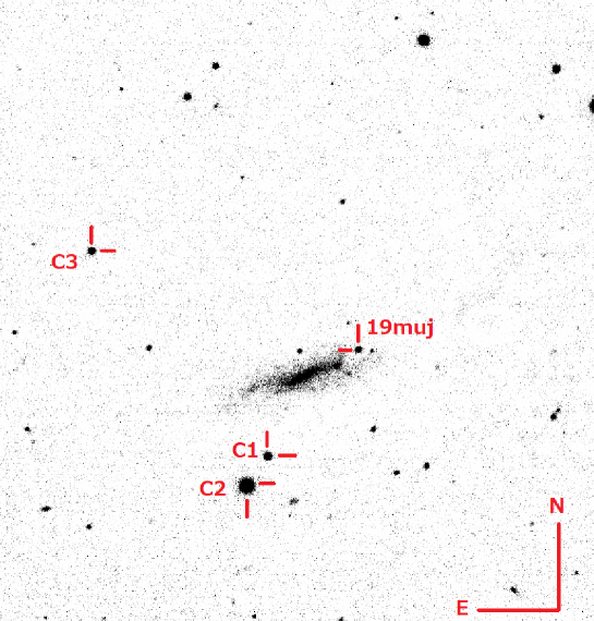
Figure 1: $R$-band image of SN 2019muj and the comparison stars taken with the Kanata telescope / HOWPol on MJD 58725.76 (2019 Aug. 30).

ccccccccc Log of optical observations of SN 2019muj. Date MJD Phase $U$ $B$ $V$ $R$ $I$ Telescope
(day) (mag) (mag) (mag) (mag) (mag) (Instrument)
Date MJD Phase $U$ $B$ $V$ $R$ $I$ Telescope
(day) (mag) (mag) (mag) (mag) (mag) (Instrument)
2019-08-08 58703.8 $-3.9$ – – 17.122 $\pm$ 0.098 17.020 $\pm$ 0.111 16.932 $\pm$ 0.109 Kanata (HONIR)
2019-08-09 58704.7 $-3.0$ – 16.947 $\pm$ 0.075 16.911 $\pm$ 0.054 16.630 $\pm$ 0.049 16.713 $\pm$ 0.053 Kanata (HOWPol)
2019-08-09 58704.8 $-2.9$ – – 16.586 $\pm$ 0.066 16.409 $\pm$ 0.085 16.421 $\pm$ 0.093 Kanata (HONIR)
2019-08-11 58706.7 $-1.0$ – – – 16.477 $\pm$ 0.023 16.467 $\pm$ 0.034 Kanata (HOWPol)
2019-08-11 58706.8 $-0.9$ – – 16.471 $\pm$ 0.079 16.332 $\pm$ 0.097 16.352 $\pm$ 0.099 Kanata (HONIR)
2019-08-12 58707.7 0.0 – – 16.173 $\pm$ 0.063 16.032 $\pm$ 0.059 15.976 $\pm$ 0.060 Kanata (HONIR)
2019-08-13 58708.7 1.1 – – 16.507 $\pm$ 0.068 16.316 $\pm$ 0.058 16.370 $\pm$ 0.030 Kanata (HONIR)
2019-08-13 58708.8 1.1 – 16.677 $\pm$ 0.041 – 16.247 $\pm$ 0.029 16.200 $\pm$ 0.069 Kanata (HOWPol)
2019-08-30 58725.7 18.0 – – 17.593 $\pm$ 0.036 17.158 $\pm$ 0.020 16.813 $\pm$ 0.045 Kanata (HONIR)
2019-08-30 58725.8 18.1 – 19.350 $\pm$ 0.076 17.667 $\pm$ 0.026 17.094 $\pm$ 0.055 16.803 $\pm$ 0.036 Kanata (HOWPol)
2019-09-04 58730.8 23.1 – – 17.849 $\pm$ 0.074 17.217 $\pm$ 0.109 – Kanata (HONIR)
2019-09-04 58730.8 23.1 – 19.396 $\pm$ 0.030 17.890 $\pm$ 0.022 17.361 $\pm$ 0.021 17.005 $\pm$ 0.032 Kanata (HOWPol)
2019-09-06 58732.7 25.1 – 19.628 $\pm$ 0.030 17.999 $\pm$ 0.024 17.442 $\pm$ 0.024 17.047 $\pm$ 0.031 Kanata (HOWPol)
2019-09-06 58732.8 25.1 – – 17.976 $\pm$ 0.092 17.475 $\pm$ 0.095 17.165 $\pm$ 0.067 Kanata (HONIR)
2019-09-14 58740.7 33.1 – – 18.344 $\pm$ 0.122 17.970 $\pm$ 0.146 17.487 $\pm$ 0.156 Kanata (HONIR)
2019-09-14 58740.8 33.1 – – – – 17.215 $\pm$ 0.030 Kanata (HOWPol)
2019-09-15 58741.8 34.1 – – 18.374 $\pm$ 0.186 17.803 $\pm$ 0.180 17.388 $\pm$ 0.118 Kanata (HONIR)
2019-09-15 58741.8 34.1 – – 18.305 $\pm$ 0.051 17.750 $\pm$ 0.082 17.427 $\pm$ 0.042 Kanata (HOWPol)
2019-09-16 58742.7 35.0 – – 18.215 $\pm$ 0.205 17.831 $\pm$ 0.128 17.425 $\pm$ 0.081 Kanata (HONIR)
2019-09-16 58742.7 35.0 – – 18.467 $\pm$ 0.081 17.954 $\pm$ 0.034 17.427 $\pm$ 0.030 Kanata (HOWPol)
2019-09-23 58749.8 42.1 – 19.696 $\pm$ 0.012 18.461 $\pm$ 0.011 17.994 $\pm$ 0.005 17.479 $\pm$ 0.012 HCT (HFOSC)
2019-09-24 58750.6 42.9 – 19.710 $\pm$ 0.030 18.499 $\pm$ 0.059 18.018 $\pm$ 0.032 17.566 $\pm$ 0.033 Kanata (HOWPol)
2019-09-25 58751.6 43.9 – 19.848 $\pm$ 0.102 18.568 $\pm$ 0.045 18.021 $\pm$ 0.042 17.555 $\pm$ 0.066 Kanata (HOWPol)
2019-09-26 58752.7 45.0 – 20.264 $\pm$ 0.246 18.626 $\pm$ 0.028 17.957 $\pm$ 0.066 – Kanata (HOWPol)
2019-10-01 58758.9 51.2 – 19.799 $\pm$ 0.023 18.605 $\pm$ 0.008 18.185 $\pm$ 0.010 17.730 $\pm$ 0.011 HCT (HFOSC)
2019-10-03 58759.6 51.9 – 19.954 $\pm$ 0.030 18.662 $\pm$ 0.041 18.192 $\pm$ 0.021 17.736 $\pm$ 0.031 Kanata (HOWPol)
2019-10-04 58760.7 53.0 – 20.105 $\pm$ 0.036 18.724 $\pm$ 0.029 18.224 $\pm$ 0.021 17.762 $\pm$ 0.031 Kanata (HOWPol)
2019-10-06 58762.6 55.0 – – 18.565 $\pm$ 0.160 18.252 $\pm$ 0.106 17.816 $\pm$ 0.063 Kanata (HONIR)
2019-10-06 58762.7 55.1 – 20.271 $\pm$ 0.224 18.803 $\pm$ 0.048 18.295 $\pm$ 0.037 17.794 $\pm$ 0.049 Kanata (HOWPol)
2019-10-08 58764.6 56.9 – – 18.644 $\pm$ 0.113 18.035 $\pm$ 0.170 17.638 $\pm$ 0.208 Kanata (HONIR)
2019-10-08 58764.7 57.0 – 20.114 $\pm$ 0.268 18.789 $\pm$ 0.039 18.297 $\pm$ 0.028 17.820 $\pm$ 0.039 Kanata (HOWPol)
2019-10-11 58767.9 60.2 – – 18.818 $\pm$ 0.015 18.313 $\pm$ 0.010 17.899 $\pm$ 0.012 HCT (HFOSC)
2019-10-16 58772.7 65.0 – 19.727 $\pm$ 0.030 19.183 $\pm$ 0.122 18.530 $\pm$ 0.060 17.956 $\pm$ 0.056 Kanata (HOWPol)
2019-10-22 58778.6 71.0 – – 18.801 $\pm$ 0.076 18.299 $\pm$ 0.090 17.707 $\pm$ 0.393 Kanata (HONIR)
2019-10-22 58778.6 70.9 – 20.255 $\pm$ 0.153 19.006 $\pm$ 0.029 18.547 $\pm$ 0.026 18.030 $\pm$ 0.057 Kanata (HOWPol)
2019-10-29 58785.6 77.9 – 20.254 $\pm$ 0.038 19.196 $\pm$ 0.075 18.639 $\pm$ 0.020 18.072 $\pm$ 0.035 Kanata (HOWPol)
2019-10-30 58786.9 79.2 – – 19.085 $\pm$ 0.023 18.662 $\pm$ 0.023 18.198 $\pm$ 0.028 HCT (HFOSC)
2019-11-06 58789.7 82.0 – 20.222 $\pm$ 0.030 19.549 $\pm$ 0.020 18.715 $\pm$ 0.045 18.148 $\pm$ 0.040 Kanata (HOWPol)
2019-11-05 58792.9 85.2 – 20.100 $\pm$ 0.040 19.182 $\pm$ 0.024 18.681 $\pm$ 0.023 18.217 $\pm$ 0.032 HCT (HFOSC)
2019-11-11 58794.6 87.0 – 19.957 $\pm$ 0.030 19.610 $\pm$ 0.271 18.928 $\pm$ 0.160 18.304 $\pm$ 0.090 Kanata (HOWPol)
2019-11-25 58808.6 100.9 – – 19.536 $\pm$ 0.058 18.944 $\pm$ 0.050 18.313 $\pm$ 0.039 Kanata (HOWPol)
2019-12-08 58825.5 117.9 – – 19.862 $\pm$ 0.033 19.315 $\pm$ 0.035 – Subaru (FOCAS)
2019-12-13 58830.6 122.9 – – 19.974 $\pm$ 0.119 19.129 $\pm$ 0.048 18.381 $\pm$ 0.049 Kanata (HOWPol)
2019-12-28 58845.5 137.8 – – – 19.123 $\pm$ 0.042 18.470 $\pm$ 0.036 Kanata (HOWPol)
2020-02-28 58907.6 199.9 – – 20.348 $\pm$ 0.056 19.634 $\pm$ 0.064 – HCT (HFOSC)

We also performed $JHK_{\rm s}$-band imaging observations with HONIR attached to the Kanata telescope, with the Nishi-harima Infrared Camera (NIC) installed at the Cassegrain focus of the 2.0 m Nayuta telescope at the NishiHarima Astronomical Observatory, and with the Near-infrared simultaneous three-band camera (SIRIUS; Nagayama et al. 2003) installed at the 1.4m IRSF telescope at the South African Astronomical Observatory. We adopted the sky background subtraction using a template sky image obtained by the dithering observation. We performed the PSF fitting photometry in the same way as used for the reduction of the optical data and calibrated the magnitude using the comparison stars in the 2MASS catalog (Persson et al. 1998). We list the journal of the NIR photometry in Table 2.1.

Log of NIR observations of SN 2019muj. Date MJD Phase $J$ $H$ $K_{\rm s}$ Telescope (day) (mag) (mag) (mag) (Instrument) 2019-08-08 58703.7 $-3.9$ 17.228 $\pm$ 0.069 – – Kanata (HONIR) 2019-08-09 58704.8 $-2.9$ 16.927 $\pm$ 0.064 17.059 $\pm$ 0.093 – Kanata (HONIR) 2019-08-10 58705.0 $-2.6$ 16.920 $\pm$ 0.045 16.944 $\pm$ 0.071 17.023 $\pm$ 0.108 IRSF (SIRIUS) 2019-08-11 58706.0 $-1.7$ 16.765 $\pm$ 0.047 16.698 $\pm$ 0.075 – IRSF (SIRIUS) 2019-08-11 58706.8 $-0.9$ 16.661 $\pm$ 0.053 16.923 $\pm$ 0.109 – Kanata (HONIR) 2019-08-12 58707.7 0.0 16.560 $\pm$ 0.060 16.753 $\pm$ 0.113 – Kanata (HONIR) 2019-08-13 58708.7 1.0 16.809 $\pm$ 0.065 – – Kanata (HONIR) 2019-08-12 58707.8 1.1 16.443 $\pm$ 0.043 17.484 $\pm$ 0.073 – Nayuta (NIC) 2019-08-14 58709.0 1.3 16.715 $\pm$ 0.047 16.616 $\pm$ 0.075 16.570 $\pm$ 0.114 IRSF (SIRIUS) 2019-08-16 58711.0 3.3 16.795 $\pm$ 0.045 16.567 $\pm$ 0.072 16.501 $\pm$ 0.113 IRSF (SIRIUS) 2019-08-17 58712.0 4.3 – 16.432 $\pm$ 0.083 16.526 $\pm$ 0.102 IRSF (SIRIUS) 2019-08-22 58717.0 9.3 16.981 $\pm$ 0.045 16.359 $\pm$ 0.071 16.562 $\pm$ 0.103 IRSF (SIRIUS) 2019-08-24 58719.0 11.3 17.034 $\pm$ 0.044 16.398 $\pm$ 0.070 16.648 $\pm$ 0.098 IRSF (SIRIUS) 2019-08-27 58722.0 14.3 17.072 $\pm$ 0.044 16.503 $\pm$ 0.070 17.084 $\pm$ 0.102 IRSF (SIRIUS) 2019-08-30 58725.7 18.0 – 16.405 $\pm$ 0.116 – Kanata (HONIR) 2019-09-02 58728.0 20.3 17.329 $\pm$ 0.044 16.770 $\pm$ 0.071 17.010 $\pm$ 0.106 IRSF (SIRIUS) 2019-09-02 58728.9 21.2 17.377 $\pm$ 0.045 16.830 $\pm$ 0.071 17.141 $\pm$ 0.116 IRSF (SIRIUS) 2019-09-03 58729.9 22.2 17.401 $\pm$ 0.046 16.832 $\pm$ 0.073 – IRSF (SIRIUS) 2019-09-04 58730.8 23.1 17.540 $\pm$ 0.113 – – Kanata (HONIR) 2019-09-14 58740.7 33.0 – 17.029 $\pm$ 0.142 – Kanata (HONIR) 2019-09-15 58741.7 34.1 – 17.167 $\pm$ 0.108 – Kanata (HONIR) 2019-09-16 58742.7 35.0 – 17.043 $\pm$ 0.166 – Kanata (HONIR) 2019-10-08 58764.6 56.9 17.838 $\pm$ 0.174 – – Kanata (HONIR) 2019-10-22 58778.6 70.9 18.681 $\pm$ 0.244 18.254 $\pm$ 0.196 – Kanata (HONIR) Relative to the epoch of $B$-band maximum (MJD 58707.69).

Additionally, we downloaded the imaging data obtained by $Swift$ Ultraviolet/Optical Telescope (UVOT) from the $Swift$ Data Archive. In the UV data of $Swift$, we adopted the absolute photometry using the zero points reported by Breeveld et al. (2011). We performed PSF fitting photometry using IRAF for these data. We list the journal of the UV photometry in Table 2.1.

Log of $Swift$/UVOT observations of SN 2019muj. Date MJD Phase $V$ $B$ $U$ $uvw1$ $uvw2$ (day) (mag) (mag) (mag) (mag) (mag) 2019-08-07 58702.8 -4.8 17.183 $\pm$ 0.139 17.406 $\pm$ 0.078 16.212 $\pm$ 0.053 16.750 $\pm$ 0.068 17.919 $\pm$ 0.093 2019-08-08 58703.8 -3.8 16.752 $\pm$ 0.097 16.952 $\pm$ 0.060 15.885 $\pm$ 0.038 16.846 $\pm$ 0.051 17.814 $\pm$ 0.089 2019-08-09 58704.6 -3.1 16.390 $\pm$ 0.073 16.787 $\pm$ 0.048 15.752 $\pm$ 0.037 16.991 $\pm$ 0.051 – 2019-08-10 58705.4 -2.3 16.472 $\pm$ 0.078 16.641 $\pm$ 0.046 15.915 $\pm$ 0.041 17.032 $\pm$ 0.053 17.906 $\pm$ 0.074 2019-08-11 58706.8 -0.9 16.602 $\pm$ 0.090 16.537 $\pm$ 0.045 15.860 $\pm$ 0.043 17.323 $\pm$ 0.065 18.196 $\pm$ 0.103 2019-08-15 58710.7 3.0 16.470 $\pm$ 0.085 16.743 $\pm$ 0.052 16.463 $\pm$ 0.058 17.914 $\pm$ 0.086 18.662 $\pm$ 0.137 2019-08-17 58712.9 5.2 16.483 $\pm$ 0.082 16.978 $\pm$ 0.060 17.079 $\pm$ 0.080 18.417 $\pm$ 0.108 19.030 $\pm$ 0.164 2019-08-25 58720.0 12.4 17.213 $\pm$ 0.151 18.374 $\pm$ 0.176 18.663 $\pm$ 0.278 19.736 $\pm$ 0.231 19.131 $\pm$ 0.219 2019-08-29 58724.3 16.6 17.062 $\pm$ 0.160 18.407 $\pm$ 0.161 18.902 $\pm$ 0.273 – 20.414 $\pm$ 0.518 2019-09-03 58729.6 21.9 17.319 $\pm$ 0.138 18.965 $\pm$ 0.246 – – – 2019-09-04 58730.0 22.3 17.552 $\pm$ 0.162 18.799 $\pm$ 0.208 – – – Relative to the epoch of $B$-band maximum (MJD 58707.69).

2.2 Spectroscopy

For the spectra taken with HOWPol, the wavelength coverage is $4500$–$9200$ Å  and the wavelength resolution is $R=\lambda/\Delta\lambda\simeq 400$ at 6000 Å. For wavelength calibration, we used sky emission lines. To remove cosmic ray events, we used the L. A. Cosmic pipeline (van Dokkum 2001; van Dokkum et al. 2012). The flux of SN 2019muj was calibrated using the data of spectrophotometric standard stars that have taken on the same night.

The spectra with KOOLS-IFU installed on Seimei telescope were taken through the optical fibers. We used the VPH-blue grism. The wavelength coverage is $4000$–$8900$ Å and the wavelength resolution is $R=\lambda/\Delta\lambda\sim 500$. The data reduction was performed using Hydra package in IRAF (Barden et al. 1994; Barden & Armandroff 1995) and a reduction software specifically developed for KOOLS-IFU data. A sky frame was separately taken, which is then subtracted from the object frame. For the wavelength calibration, we used the arc lamp (Hg and Ne) data.

For the spectrum obtained with FOCAS, the wavelength coverage is $3700$–$10000$ Å and the wavelength resolution is $R=\lambda/\Delta\lambda\sim 650$ at 6000 Å. The data reduction was performed in the same way as that with HOWPol, except that we used the arc lamp (Th-Ar) data and skylines for the wavelength calibration. The journal of spectroscopy is listed in Table 2.2.

Log of the spectroscopic observations of SN 2019muj. Date MJD Phase Coverage Resolution Telescope (day) (Å) (Å) (Instrument) 2019-08-08 58703.7 $-4.0$ $4000$–$8900$ 500 Seimei (KOOLS) 2019-08-10 58705.7 $-2.0$ $4000$–$8900$ 500 Seimei (KOOLS) 2019-08-11 58706.7 $-1.0$ $4000$–$8900$ 500 Seimei (KOOLS) 2019-08-11 58706.8 $-0.9$ $4500$–$9200$ 400 Kanata (HOWPol) 2019-08-16 58711.7 4.1 $4000$–$8900$ 500 Seimei (KOOLS) 2019-08-17 58712.7 5.0 $4000$–$8900$ 500 Seimei (KOOLS) 2019-08-21 58716.7 9.0 $4000$–$8900$ 500 Seimei (KOOLS) 2019-09-05 58731.7 24.0 $4000$–$8900$ 500 Seimei (KOOLS) 2019-09-23 58749.8 42.1 $3500$–$9000$ 300 HCT (HFOSC) 2019-09-24 58750.7 43.0 $4000$–$8900$ 500 Seimei (KOOLS) 2019-09-25 58751.7 44.0 $4000$–$8900$ 500 Seimei (KOOLS) 2019-09-25 58751.7 44.0 $4500$–$9200$ 400 Kanata (HOWPol) 2019-10-11 58767.9 60.2 $3500$–$9000$ 300 HCT (HFOSC) 2019-10-31 58787.8 80.1 $3500$–$9000$ 300 HCT (HFOSC) 2019-11-06 58793.6 85.9 $3500$–$9000$ 300 HCT (HFOSC) 2019-12-08 58825.5 117.8 $3700$–$6000$ 650 Subaru (FOCAS) 2019-12-08 58825.5 117.8 $5800$–$10000$ 650 Subaru (FOCAS) Relative to the epoch of $B$-band maximum (MJD 58707.69).

3 Results

3.1 Light Curves

Figure 2 shows the multi-band light curves of SN 2019muj, from the rising phase through the tail phase. We compare the $V$-band light curves of SN 2019muj and other SNe Iax in Figure 3. We estimate the epoch of the $B$-band maximum as MJD 58707.69 $\pm$ 0.07 (2019 Aug. 12.7) by performing a polynomial fitting to the data points around the maximum light. In this paper, we refer the $B$-band maximum date as 0 days.

We derive the maximum magnitudes in the $B$ and $V$ bands as 16.623 $\pm$ 0.025 mag and 16.380 $\pm$ 0.018 mag, respectively. The distance modulus for VV525 is taken as $\mu=$ 32.46 $\pm$ 0.23 mag, which is the mean value of the results from different methods, as summarized in the NASA/IPAC Extragalactic Database (NED). The extinction through the Milky Way is estimated as $E(B-V)=0.023$ mag (Schlafly & Finkbeiner 2011) for which we adopt $R_{V}=3.1$. We assume negligible extinction within the host galaxy, based on the absence of the Na D lines and the color evolution as compared with those of other SNe Iax. The $B$-band absolute peak magnitude of SN 2019muj is then $-16.323\pm 0.23$ mag. SN 2019muj is fainter by $\sim$ 1.5 mag than SNe 2002cx ($-17.55\pm 0.34$ mag; Li et al. 2003) and 2005hk ($-18.02\pm 0.32$ mag; Sahu et al. 2008). On the other hand, SN 2019muj is brighter than SNe Iax 2008ha ($-13.74\pm 0.15$ mag; Foley et al. 2009, $-13.79\pm 0.14$ mag; Stritzinger et al. 2014) and 2010ae ($-13.44\sim-15.47$ mag; Stritzinger et al. 2014).

We derive the decline rate of SN 2019muj in the $B$ and $V$ bands as $\Delta$m₁₅($B$) = 2.16 $\pm$ 0.21 mag and $\Delta$m₁₅($V$) = 1.18 $\pm$ 0.04 mag, respectively. The $B$-band decline rate is similar to SNe 2008ha (2.17 $\pm$ 0.02 mag; Foley et al. 2009, 2.03 $\pm$ 0.20 mag; Stritzinger et al. 2014) and 2010ae (2.43 $\pm$ 0.11; Stritzinger et al. 2014). This value is larger than those of the brighter SNe Iax 2002cx (1.29 $\sim$ 0.11 mag; Li et al. 2003) and 2005hk (1.56 $\pm$ 0.09 mag; Sahu et al. 2008).

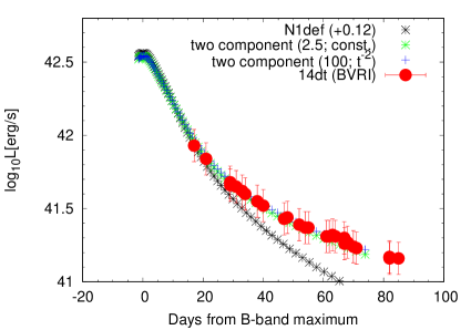
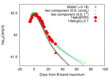
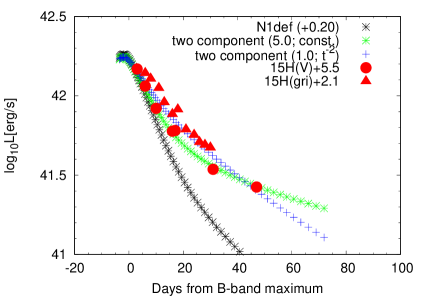
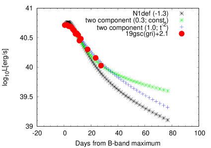
Figure 16: The same as Figure 13 but for different SNe Iax.

Figure 4 shows the relationship between the peak absolute magnitude in the $V$ band and the decline rate $\Delta m_{15}$($V$). The decline rate of SN 2019muj is similar to those of subluminous SNe Iax 2008ha and 2010ae. The peak magnitude is however between the subluminous SNe Iax and bright SNe Iax. SN 2019muj thus belongs to the intermediate subclass between the bright and subluminous SNe Iax, similar to SNe 2004es and 2009J (Figure 16 of Foley et al. 2013). Barna et al. (2021) also pointed out that SN 2019muj is located at the luminosity gap for SNe Iax. For the intermediate SNe Iax, multi-band data covering the rising phase are still limited. We discuss the light curve in the rising phase in §4.1.

After $\sim$30 days, the evolution of the light curve becomes slow. The decline rates in $V$, $R$, and $I$-band light curves between 100 – 200 days are calculated 0.007 $\pm$ 0.002, 0.005 $\pm$ 0.003, and 0.004 $\pm$ 0.001 mag, respectively. We compare the light curves of SN 2019muj with those of SN 2014dt after 60 days. Their decline rates exhibit impressive similarity. In §4, we focus on the late-phase light curves and provide analytical inspection. SN 2019muj is the second case which clearly shows a slowly evolving light curve, being consistent with the full trapping of the $\gamma$-ray energy from ⁵⁶Co decay (see also §4.3).

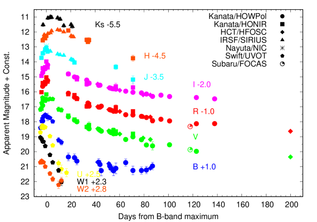
Figure 2: Multi-band light curves of SN 2019muj. The different symbols denote data that were obtained using different instruments (see the figure legends). The light curve of each band is shifted vertically as indicated in the figure. We adopt MJD 58707.69 $\pm$ 0.07 as 0 days.

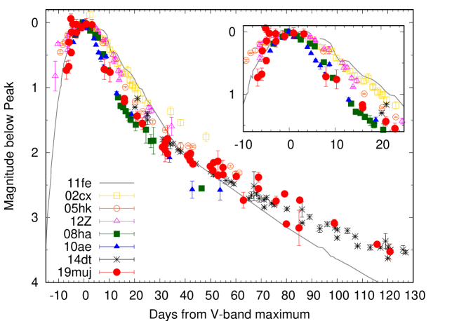
Figure 3: $V$-band light curve of SN 2019muj. For comparison, we plot those of SNe 2002cx (Li et al. 2003), 2005hk (Sahu et al. 2008), 2008ha (Foley et al. 2009), 2010ae (Stritzinger et al. 2014), 2011fe(Zhang et al. 2016), 2012Z (Yamanaka et al. 2015), and 2014dt (Kawabata et al. 2018).

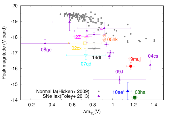
Figure 4: Relationship of the peak absolute magnitude in the $V$ band with the decline rate $\Delta m_{15}$($V$). The gray points are the data of normal SNe Ia (Hicken et al. 2009), and the other points are for SNe Iax (Li et al. 2003, Phillips et al. 2007, Sahu et al. 2008, Foley et al. 2009, McClelland et al. 2010, Foley et al. 2013, Stritzinger et al. 2014, Stritzinger et al. 2015, Yamanaka et al. 2015, Kawabata et al. 2018). For some SNe Iax, the SN IDs are given by labels.

3.2 Spectral Evolution

We show the optical spectra of SN 2019muj from $-4.0$ days through $117.8$ days in Figures 5 – 8. In the spectra before the $B$-band maximum light, SN 2019muj shows a blue continuum with the narrow absorption lines of Si ii, S ii, Fe iii and C ii (Figures 5 and 6). Although some of the spectra of SN 2019muj are somewhat noisy, it is clearly seen that the C ii absorption line is as strong as the Si ii $\lambda$ 6355 line during the early phases. SN 2019muj is similar to SNe 2008ha and 2010ae in many spectral features (except for Si ii, Ca ii IR triplet) including narrow absorption lines.

After the $B$-band maximum light, SN 2019muj shows the absorption lines of Na i D, Fe ii, Fe iii, Co ii, and the Ca ii IR triplet (Figures 5 and 7). These absorption lines of SN 2019muj are narrow, similarly to those seen in the pre-maximum spectra. SN 2008ha and SN 2010ae have similar spectra around maximum light (see Stritzinger et al. 2014).

The late phase spectrum ($\sim$ 120 days) of SN 2019muj is plotted in Figure 8. SN 2019muj shows the narrow permitted Fe ii lines and several forbidden lines associated with Fe, Co, and Ca ii. The line identification is based on Jha et al. (2006) and Sahu et al. (2008). In this phase, there are few comparative samples of SNe Iax. Once the spectrum of SN 2019muj is smoothed using the Gaussian function with a kernel width of 10 pixels ($\sim 500$ km s^-1), and then shifted to the blue by $\sim$ 900 km s^-1 (Figure 8), the similarity to SN 2014dt is striking. The spectrum of SN 2019muj in the late phase is thus characterized by low velocities, being consistent with its similarities to SN 2010ae in the earlier phase.

We obtained the line velocity of Si ii $\lambda$ 6355 by performing a single-Gaussian fit to the absorption line profile using the splot task in $IRAF$. We determined the uncertainty as the root mean square sum of the standard deviation in the fits and the wavelength resolution. In Figure 9, we show the velocity evolution of Si ii $\lambda$ 6355. At $-4.0$ days, the line velocity of Si ii is 4,590 $\pm$ 610 km s^-1. It is slower than that of SN 2005hk ($\sim$ 6,000 km s^-1; Phillips et al. 2007), while it is similar to SN 2010ae ($\sim$ 4,500 km s^-1; Stritzinger et al. 2014). Around maximum light, the line velocity is 4,430 $\pm$ 750 km s^-1, which is again similar to the velocity of SN 2010ae ($\sim$ 4,500 km s^-1; Stritzinger et al. 2014). SN 2019muj has faster line velocities than faint SN 2008ha.

In summary, SN 2019muj shows the narrow lines and slow expansion velocity. Its spectroscopic features are similar to those of subluminous SNe Iax such as SNe 2008ha and 2010ae. The photometric properties of SN 2019muj are consistent with those of the intermediate SNe Iax. Note that spectra of the intermediate SNe Iax are similar to those of subluminous ones.

Figure 5: Spectra evolution of SN 2019muj. The epoch of each spectrum is indicated on the right outside the panel. The gray line connects the position of the Si ii $\lambda$ 6355 line as a function of time.

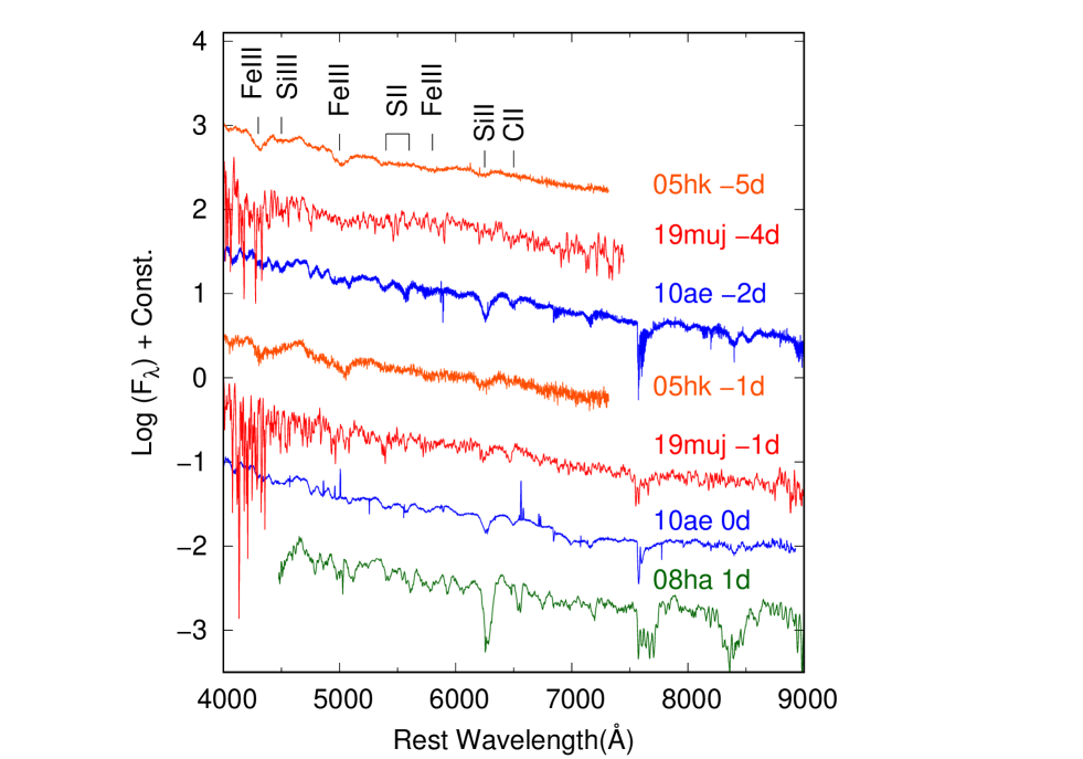
Figure 6: Spectral comparison of SN 2019muj with other SNe Iax; 2005hk (Blondin et al. 2012), 2008ha (Valenti et al. 2009), 2010ae (Stritzinger et al. 2014). The phase of these spectra is from $\sim-5$ days to around the maximum light.

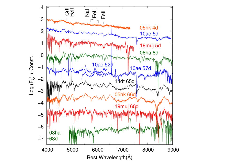
Figure 7: Spectral comparison of SN 2019muj with other SNe Iax; 2005hk (Phillips et al. 2007; Blondin et al. 2012), 2008ha (Valenti et al. 2009; Foley et al. 2009), 2010ae (Stritzinger et al. 2014). The phase of these spectra is from $\sim$ 5 days to $\sim$ 60 days.

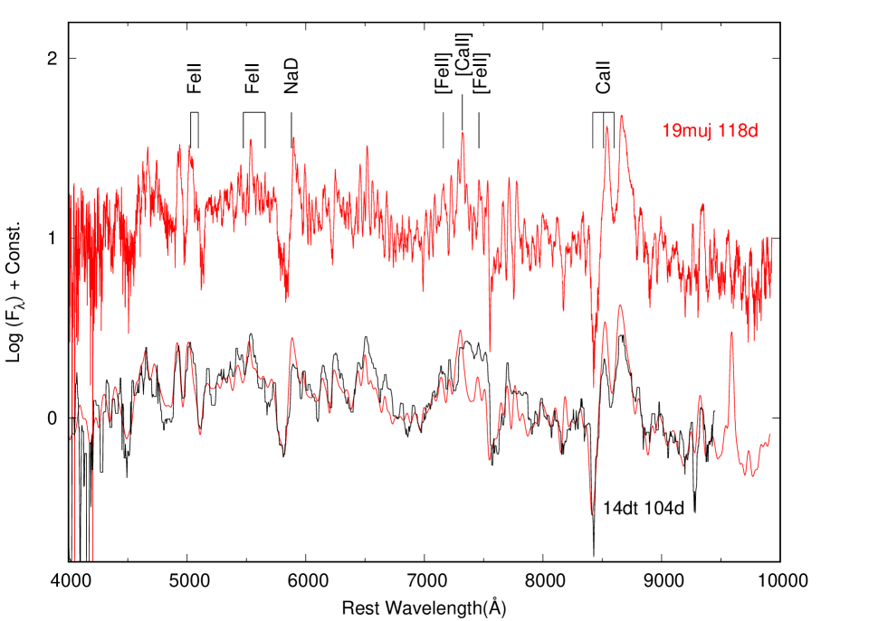
Figure 8: Late-phase spectra of SN 2019muj (red lines) and SN 2014dt (black lines; Kawabata et al. 2018). We overplot the Gaussian smoothed and blue-shifted spectrum of SN 2019muj on the spectrum of SN 2014dt.

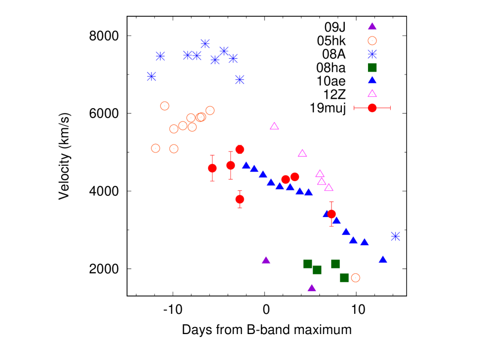
Figure 9: Evolution of the line velocity of Si ii $\lambda$ 6355 in SN 2019muj. For comparison, we plotted those for SNe 2009J, 2005hk, 2008A, 2008ha, 2010ae, and 2012Z.

4 Discussion

SN 2019muj shows the fast decline in the early phase and the narrow absorption lines similar to subluminous SNe Iax. We classify it as an intermediate-luminosity SN Iax based on its relatively bright peak magnitude. SN 2019muj is the second case which clearly shows a slow evolution of the light curve in the late phase, following bright SN Iax 2014dt (Kawabata et al. 2018). Then, it is a good target for testing the weak deflagration scenario. We also apply the analytical method to other SNe Iax, and examine whether their light curves can be reproduced or not.

4.1 Early Light Curves

From the light curves covering the rising phase through the peak phase, we constrain the explosion date and the rise time in the same way as was done by Kawabata et al. (2020). We assume the homologously expanding “fireball model” (Arnett 1982; Riess et al. 1999; Nugent et al. 2011) to estimate the explosion date. In this model, the luminosity/flux ($f$) increases as $f\propto t^{2}$, where $t$ is the time since the zero points. In this paper, we assume that the zero points in the time axis in this relation is the same for different bands (i.e., the explosion date), and adopt the same power-law index of 2 in all the $BVRI$ bands.

In Figure 10, we show the early $BVRI$-band light curves fitted by the fireball model only with our data. The rising behavior of SN 2019muj in all the bands can be explained by this simple fireball model. Through the fitting, we estimate the explosion date as MJD 58694.59 $\pm$ 2.1. Note that the accuracy of the fit may depend on the temporal coverage of the data points used in the fit, and the error in the explosion date estimate above takes into account the change due to this effect; the final data phase included in the fit is varied by a few days. As a cross-check, we also overplotted the discovery magnitude and the non-detection, upper-limit magnitude. These ASAS-SN points, as obtained in the $g$ band, were not used in the fit. Given the difference of $\sim$ 0.3 mag between the $B$ and $g$ bands, their points are consistent with the fireball model. No excess is found beyond the fireball prediction. However, it should be noted that there is not very much data sufficiently in the early phase to test the light curve behavior in the first week of the explosion.

The rise time, defined as the time interval between the explosion date and maximum date, may also provide some insights into the explosion property. Its correlations with other observational features have been investigated for normal SNe Ia (e.g., Hayden et al. 2010; Ganeshalingam et al. 2010; Jiang et al. 2020). This has also been investigated for SNe Iax (Magee et al. 2016). The rise time of SN 2019muj in the $B$ band is 13.1 $\pm$ 2.1 days. Magee et al. (2016) reported a correlation between the peak absolute magnitude and the decline rate either in the $R$ or $r$ band. Because of the missing data around maximum light in the $R$ band, we assume that the color evolution of SN 2019muj is similar to that of other SNe Iax. Then, we convert the rising time in the $B$ band to that in the $R$ band. We thereby estimate the $R$-band rise time of SN 2019muj as 16 – 21 days. In Figure 5 in Magee et al. (2016), SN 2019muj is located between bright SNe Iax and subluminous ones, following the relation found by Magee et al. (2016).

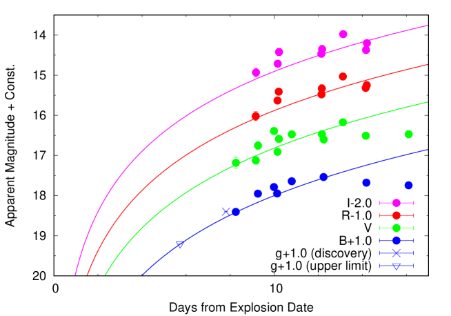
Figure 10: Optical light curve of SN 2019muj at the early phase. We also plot the discovery magnitude and upper-limit magnitude reported by Brimacombe et al. (2019), which were obtained in the $g$ band. The explosion date is estimated to be MJD 58692.54 using the quadratic function (§4.1).

4.2 Explosion Parameters

We derived the bolometric luminosity of SN 2019muj by interpolating the SED and integrating the fluxes within the optical bands. The derived bolometric light curve is shown in Figure 11. SN 2019muj has intermediate luminosity among SNe Iax. With the peak luminosity and the rising time, we estimate the mass of the synthesized ⁵⁶Ni (Arnett 1982; Stritzinger & Leibundgut 2005) as 0.01 – 0.03 $M_{\odot}$, using the rise time and the peak bolometric luminosity as 13.1 $\pm$ 2.1 days and (0.3 – 0.8) $\times 10^{41}$ erg s^-1, respectively. The estimated ⁵⁶Ni mass is consistent with the value reported by Barna et al. (2021).

We then estimate $M_{\rm ej}$ and $E_{\rm k}$ of the ejecta of SN 2019muj by applying the scaling laws,

$$t_{\rm d}\propto\kappa^{1/2}\ M_{\rm ej}^{3/4}\ E_{\rm k}^{-1/4}\mbox{, and}$$ (1)

$$v\propto E_{\rm k}^{1/2}\ M_{\rm ej}^{-1/2}\mbox{,}$$ (2)

where $t_{\rm d}$ is the diffusion timescale ($\sim$ light curve width in the early phase), $\kappa$ is the absorption coefficient for optical photons, and $v$ is the typical expansion velocity of the ejecta. Here, we calibrate the relations by the properties of the well-studied SN Ia 2011fe (Pereira et al. 2013) to anchor the normalization. We then obtain $E_{k,19muj}$ $\sim$ 0.02 – 0.19 $\times$ $10^{50}$ erg, $M_{ej,19muj}$ $\sim$ 0.16 – 0.95 $M_{\odot}$ and $\kappa_{19muj}$ / $\kappa_{11fe}$ $\sim$ 0.7 – 4.1 (see Kawabata et al. 2018 for details).

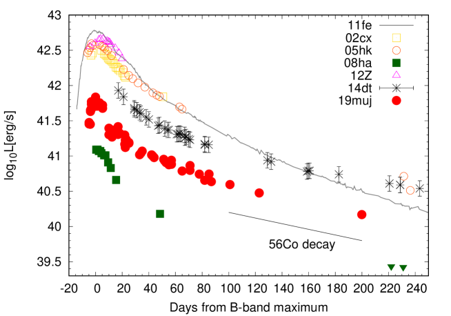
Figure 11: Bolometric light curve of SN 2019muj. For comparison, we plotted the light curves of SNe 2002cx (Li et al. 2003), 2005hk (Sahu et al. 2008), 2008ha (Foley et al. 2009; Foley et al. 2010), 2011fe (Zhang et al. 2016), 2012Z (Yamanaka et al. 2015), and 2014dt (Kawabata et al. 2018).

4.3 Comparison to the Weak Deflagration Model

For SNe Iax, some explosion models have been proposed. Among those models is the weak deflagration model leaving a bound WD remnant after the explosion; in this model, changing the number of ignition spots or the initial composition of the WD can explain the observational properties from bright SNe Iax to subluminous ones like SN 2008ha (Fink et al. 2014; Kromer et al. 2015). In this section, we compare the observational properties of SN 2019muj to the expectations from this particular explosion model. In the present work, we focus on the light curve behavior; the spectroscopic properties have been investigated by Barna et al. (2021), who showed that the weak/failed deflagration model can roughly explain the early-phase spectral evolution while the degree of abundance mixing found for SN 2019muj (or SNe Iax in general) is not as substantial as expected by the model.

In the model sequence of Fink et al. (2014), the models N1def, N3def, and N5def cover the explosion parameters constrained for SN 2019muj (see §4.2). In Figure 12, we compare the bolometric light curve of SN 2019muj and the light curves calculated for these models. The bolometric light curve of SN 2019muj is similar to that expected from the N1def model, while the peak luminosity of SN 2019muj is slightly fainter than the N1def model (see also Barna et al. 2021). Then, we try to match the light curve of the N1def model to that of SN 2019muj around the peak by shifting the model luminosity. This modified model can reproduce the light curve of SN 2019muj until $\sim$ 20 days. However, in the tail phase, SN 2019muj shows the slow decline, unlike the model light curves that fade away very quickly.

To explain the light curve in the late phase, an additional energy source is required. In the model sequence by Fink et al. (2014), they indeed predict the presence of a bound WD remnant, which contains some ⁵⁶Ni. To test this hypothesis further, we first calculate the decline rate in the late phase by fitting a linear function to the bolometric light curve. The decline rate is found to be $\sim$ 0.004 dex day^-1 (0.01 mag day^-1) between 60 – 210 days, which matches the expectation from nearly full-trapping of the $\gamma$-rays. This indicates that the additional component is powered by the decay of ⁵⁶Co within a high-density inner component.

This additional contribution is not directly included in the model light curves of Fink et al. (2014). Indeed, the radiation process regarding this bound remnant has not been well understood (e.g., Foley et al. 2016). There are several possible scenarios in which the bound WD remnant would create the inner dense component: (1) It is possible that the component is indeed a static bound WD remnant itself. (2) Alternatively, the bound WD could create the inner ejecta with a slow expansion velocity, which may behave like the additional inner dense component due to its high density. (3) Finally, there is a possibility that a high-density wind is launched from a bound WD remnant (Foley et al., 2016).

Here, we consider a simple and phenomenological model (Kawabata et al. 2018) where the power from ⁵⁶Ni in the bound remnant is anyway radiated away through a dense environment (either in the static WD, slowly moving inner ejecta, or a possible wind), without much energy loss nor time delay. As the bolometric luminosity in the late phase, we thus consider the simple radioactive-decay light curve model (Maeda et al. 2003).

$$L_{\rm bol} = M(^{56}$$ Ni)_in [ e^(-t/8.8 d) ϵ_γ,Ni (1 - e^-τ) (3)

$$+\left.e^{(-t/111{\rm\ d})}\left\{\epsilon_{\gamma,\rm Co}(1-e^{-\tau})+\epsilon_{e^{+}}\right\}\right]$$

where $\epsilon_{\gamma,\rm Ni}=3.9\times 10^{10}$ erg s^-1 g^-1 is the energy deposition rate by ⁵⁶Ni via $\gamma$-rays, $\epsilon_{\gamma,\rm Co}=6.8\times 10^{9}$ erg s^-1 g^-1 and $\epsilon_{e^{+}}=2.4\times 10^{8}$ erg s^-1 g^-1 are those by the ⁵⁶Co decay via $\gamma$-rays and positron ejection. The optical depth of the inner component, $\tau$, will evolve with time differently for the different scenarios for the inner component; this is expected to be constant for the bound WD, or to evolve as $\tau\propto t^{-2}$ for the slowly moving ejecta. These two possibilities will be examined below. In the case of the WD wind, the evolution is not trivial, but it likely decreases with time as the mass-loss rate goes down; it is probably a reasonable guess that the rate of the decrease for the wind case is between the two cases mentioned above. Note that $M$(⁵⁶Ni)_in and the optical depth here refer to those of the inner component alone without the outer component estimated in §4.2.

We then add this additional component to the model light curve of Fink et al. (2014). In Figure 12, we show this combined light curve model. The mass of ⁵⁶Ni in the inner component is derived as $\sim$ 0.018 M_⊙. For the case of the constant optical depth, we have derived $\tau$ $\sim$ 5.0. $\tau$ is the lower limit, and any value larger than this does not affect the change in the bolometric luminosity. For the case of the slow-moving inner ejecta, the optical depth is characterized as follows;

$$\tau\simeq 1000\times\left[\frac{(M_{\rm ej}/M_{\odot})^{2}}{E_{51}}\right]_{in}\left(\frac{t}{\mbox{day}}\right)^{-2}\mbox{ ,}$$ (4)

$M_{\rm ej}$ is the ejecta mass, and $E_{51}$ is the kinetic energy in $10^{51}$ erg (both only for the inner component). We can reproduce the light curve with [$(M_{\rm ej}/M_{\odot})^{2}/{E_{51}}$]_in $\sim$ 100. The analysis here indicates the existence of the inner dense component, irrespective of the specific scenarios for its origin. The high-density component in the inner part was also seen in the bright SN Iax 2014dt thought similar analysis (Kawabata et al. 2018); we thus find this inner component as a common property shared by bright and intermediate luminosity SNe Iax.

As shown above, the light curve is well reproduced irrespective of the evolution of the optical depth. In other words, from this analytical model of the bolometric light curve, it is difficult to distinguish the scenarios for the origin of the inner component. This stems from the observed decay rate following the full trapping of the $\gamma$-rays; as long as $\tau\gg 1$, the result is not dependent on the time evolution of the optical depth. Indeed, in the model for the slowly moving ejecta, the optical depth will decrease below unity $\sim$ one year after the explosion. Therefore, further following the light curve evolution even longer than the observation in the present work may be useful to distinguish at least the slowly moving ejecta scenario. Also, the spectral evolution in the late phase is a key to addressing this question.

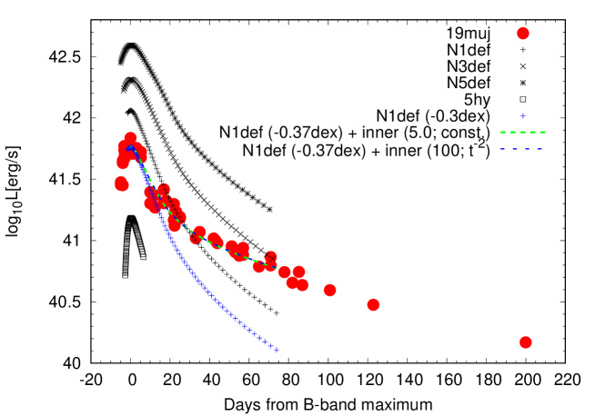
Figure 12: Bolometric light curve of SN 2019muj. We compare the the weak deflagration model light curve (black points; Fink et al. 2014, Kromer et al. 2015), N5def, N3def N1def, and N5hybrid respectively. The blue points are the N1def model shifted downward to fit the peak luminosity of SN 2019muj. The green and blue dashed lines are the two-component model as the sum of the weak deflagration model and the simple radioactive-decay light curve model (see §4.3); the evolution of the optical depth is taken as either $\tau=$ constant (green) or $\tau\propto t^{-2}$ (blue).

4.4 Bound WD Remnants in all SNe Iax?

In this section, we expand the analysis in §4.3 on the light curve behavior to a sample of SNe Iax. We estimate the bolometric luminosities of these SNe Iax using the same method as adopted for SN 2019muj (see Appendix for further details). In Figure 13, 14, 15 and 16, we compare the bolometric light curves of SNe Iax and those predicted by Fink et al. (2014) for the weak deflagration model series. We can find a subset of the model series that can fit the early phase light curve of individual SNe Iax. However, the models can not replicate the late-phase slow evolution seen in the observed light curves, as is similar to the case for SN 2019muj, except for SNe 2011ay and 2019gsc. Since their models do not consider the inner-part ejecta components, we further consider the light curve model with a variety of the inner-part ejecta properties (see §4.3) to fit the bolometric light curves of other SNe Iax. Using the same methodology as in §4.3, we try to fit the combined light curve model with the two cases where $\tau$ is either constant (i.e., the static remnant) or evolve as $\tau\propto t^{-2}$ (i.e., the slowly moving inner ejecta). Their light curves are well reproduced by this model sequence (Figure 13, 14, 15, and 16). Again, similarly to the case for SN 2019muj, we unfortunately can not constrain the time evolution of the optical depth with the available data set. This highlights the importance of observations in even later phases (§4.3).

Most of SNe Ia are found to have a high-density component in the innermost layer according to the above analyses. Extremely long-term photometric observations are available for a few SNe Iax (SN 2008ha; Foley et al. 2014, SN 2012Z; McCully et al. 2021), which show slowly decaying light curves even in the extremely late phases ( $\geq$ 1400 days). These observations are consistent with our analysis, and probably support the presence of the inner component. The very slow decay even in such a late phase may disfavor the possibility of the homologously expanding inner ejecta as an origin of the inner-dense component. However, the luminosity in the very late phase may indeed decrease even more slowly than the radioactive decay, which might require an additional power source, e.g., CSM interaction (McCully et al., 2021); then it wold not provide a strong constraint on the evolution of the optical depth of the inner component. Further observation and analysis covering the full evolution of SNe Iax will help understand their nature.

The explosion simulations by Fink et al. (2014) predict the ⁵⁶Ni masses in the inner and outer layers for a given set of input parameters to characterize the explosion. In Table 4.4, we show the parameters obtained by our fit to the observed light curves. The ⁵⁶Ni masses required to fit the late-phase light curves are substantially larger than the model predictions. Especially, SNe 2009ku and 2008ge show large discrepancies.

An additional issue is that we do not see a correlation between the properties of the outer ejecta and the inner component expected in the explosion simulations. Figure 17 shows the relationship between the obtained ⁵⁶Ni mass in the outer layer and that in the inner layer. Fink et al. (2014) predicted that the model with a larger amount of ⁵⁶Ni in the outer ejecta has less ⁵⁶Ni mass in the inner layer. However, our results do not follow a clear correlation. This discrepancy indicates that there may still be missing functions in the explosion mechanism of SNe Iax and the origin(s) of their diverse properties that we have not considered in our current analysis.

We also check if there is a relation between the ejecta mass in the outer layer and the optical depth in the inner component. In the model calculation by Fink et al. (2014), for a smaller explosion energy, the bound WD mass becomes larger and the outer ejecta mass becomes smaller. The combination of the larger WD mass and smaller explosion energy likely leads to a larger optical depth of the inner component along with this scenario, while the detail will be dependent on the specific origin for the inner component. We may anyway expect, at least roughly, an anti-correlation between the outer ejecta mass and the inner optical depth. We show this exercise in Figure 18. We do not see a clear relation between the two parameters. Similarly to the conclusion reached by the non-correlation between the ⁵⁶Ni masses in the inner and the outer components, the finding here would further indicate that an important function is still missing in our analysis or in our understanding of the nature of SNe Iax.

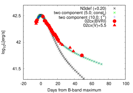
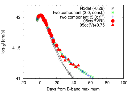
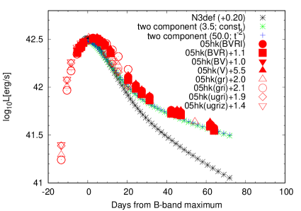
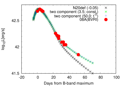
Figure 13: Bolometric light curves of SNe Iax (red points). We compare the weak deflagration model light curve (black points; Fink et al. 2014). The black points are shifted to fit the peak luminosity of each SN Iax. The green and blue points are the two-component model as the sum of the weak deflagration model and the simple radioactive-decay light curve model (see §4.3); the evolution of the optical depth is taken as either $\tau=$ constant (green) or $\tau\propto t^{-2}$ (blue).

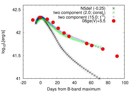
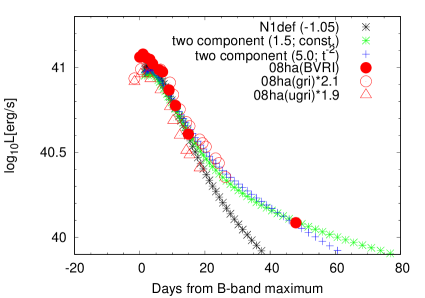
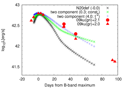
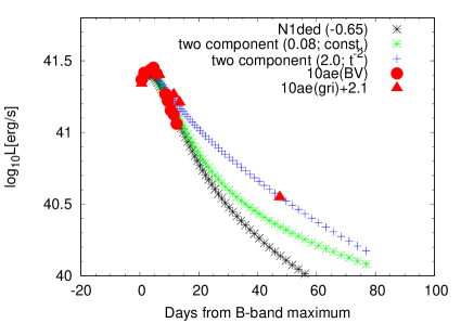
Figure 14: The same as Figure 13 but for different SNe Iax.

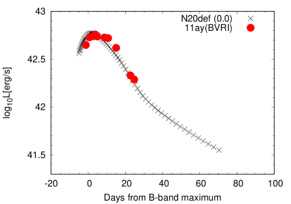
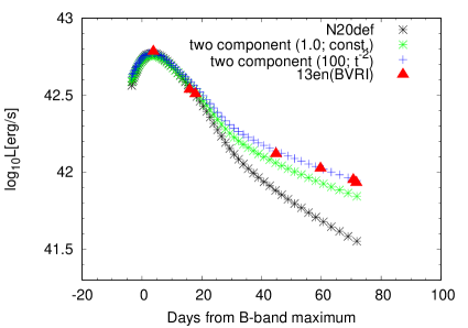
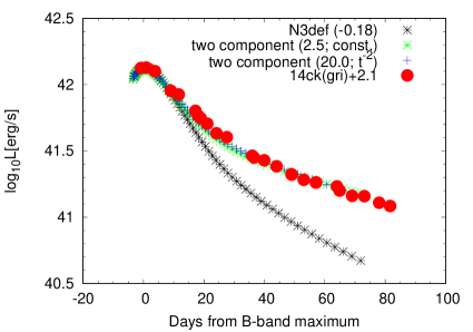
Figure 15: The same as Figure 13 but for different SNe Iax.

Figure 17: Relationship between the ⁵⁶Ni mass in the outer layer and that in the inner layer (filled circles). The asterisk symbols denote the ⁵⁶Ni masses calculated by Fink et al. (2014).

Figure 18: Relationship between the ejecta mass in the outer layer and the optical depth in the inner component. For the optical depth, the two cases are shown; $\tau=$ constant (right panel) or $\tau\propto t^{-2}$ (left panel). For the latter case, the optical depth is given at 70 days after the explosion.

Data sets of SNe Iax and the properties. SN L_peak $\tau$ [$(M_{\rm ej}/M_{\odot})^{2}/{E_{51}}$]_in M⁵⁶Ni_out M⁵⁶Ni_in Distance E($B-V$) Band References ($10^{42}$ erg/s) (Mpc) (mag) 2002cx 3.2 5.0 1.6 0.007 0.038 104.2 0.034 $BVRI$ 1 2005cc 1.1 3.0 0.8 0.084 0.020 37.0 0.0056 $BVRI$ 2,3,4,5 2005hk 3.6 3.5 7.9 0.065 0.029 49.2 0.11 $BVRI$ $ugriz$ 6,7,8 2008A 5.4 3.5 7.4 0.267 0.030 70.0 0.0427 $BVRI$ 9 2008ge 2.5 2.0 2.3 0.175 0.278 16.8 0.0109 $V$ 10 2008ha 0.1 1.5 0.8 0.074 0.043 21.3 0.075 $BVRI$ $ugri$ 11,12 2009ku 5.0 0.3 0.6 0.278 0.829 370.0 0.0063 $gri$ 13 2010ae 0.3 0.1 0.3 0.062 0.072 13.1 0.62 $BV$ $gri$ 14 2011ay 6.0 – – 0.017 – 86.9 0.081 $BVRI$ 15 2012Z 4.5 1.5 0.7 0.271 0.122 30.2 0.036 $BVRI$ $ugri$ 16,17 2013en 6.3 1.0 14.9 0.266 0.091 66.2 0.5 $BVRI$ 18 2014ck 3.2 2.5 3.2 0.083 0.045 24.4 0.48 $gri$ 19 2014dt 1.2–1.8 2.5 16.6 – 0.020 14.5 0.02 $BVRI$ 20 2014ek 3.2 0.6 0.8 0.071 0.039 99.5 0.054 $BVRI$ $gri$ 21 2015H – 5.0 0.5 0.038 0.049 60.57 0.048 $V$ $gri$ 22 2019gsc 0.025 0.3 0.2 0.086 0.100 39.8 0.01 $gri$ 23 2019muj 0.5 5.0 16.6 0.047 0.018 32.46 0.023 $BVRI$ 24 (1) Li et al. (2003); (2) Ganeshalingam et al. (2010); (3) Silverman et al. (2012); (4) Lennarz et al. (2012); (5) Foley et al. (2013); (6) Sahu et al. (2008); (7) Holtzman et al. (2008); (8) Lennarz et al. (2012); (9) Hicken et al. (2012); (10) Foley et al. (2010); (11) Foley et al. (2009); (12) Stritzinger et al. (2014); (13) Narayan et al. (2011); (14) Stritzinger et al. (2014); (15) Szalai et al. (2015); (16) Stritzinger et al. (2015); (17) Yamanaka et al. (2015); (18) Liu et al. (2015); (19) Tomasella et al. (2016); (20) Kawabata et al. (2018); (21) Li et al. (2018); (22) Magee et al. (2016); (23) Srivastav et al. (2020); (24) This work.

5 Conclusions

We presented a long-term observation of SN 2019muj. Based on the photometric properties of SN 2019muj, it belongs to the intermediate subclass between the bright and subluminous SNe Iax (see also Barna et al. 2021). The spectroscopic features are similar to those of subluminous SNe Iax such as SNe 2008ha and 2010ae, with narrow absorption lines and slow expansion velocity. The similarity between the intermediate and subluminous subclasses in the spectroscopic features is in line with the previous work (e.g., Stritzinger et al. 2014). Our long-duration observations covering the epochs until $\sim$200 days after the B-band maximum show that SN 2019muj exhibits slow evolution of the light curve in the late phase. This behavior is similar to what was previously found for the bright SN Iax 2014dt. Our observational data for SN 2019muj, including the multi-band data from the rising phase, serve as reference data set for a class of the intermediate SNe Iax, given that such well-sampled data are still limited for this class.

We estimated that the ⁵⁶Ni mass was 0.01 – 0.03 $M_{\odot}$, the kinetic energy was $\sim$ (0.02 – 0.19) $\times$ $10^{50}$ erg, and the ejecta mass was $\sim$ 0.16 – 0.95 $M_{\odot}$. These values are consistent with the prediction of the weak deflagration model.

The slow evolution in the late phase is best explained by an additional high-density component in the innermost layer. We reproduced the entire bolometric light curves of SN 2019muj and a sample of SNe Iax from the early to late phases, by adopting a phenomenological light curve model where we added an inner dense component powered by ⁵⁶Ni, with the optical depth and ⁵⁶Ni mass treated as free parameters. The model can explain the light curves of SNe Iax in general, which might support the existence of a high-density component in most, if not all, of SNe Iax. The currently available data set is however not sufficient to further specify the origin of this inner component; this could be either the remnant WD itself, the slowly moving inner ejecta, or a wind launched from the WD. In any case, the remnant WD would likely create an inner dense component, and thus the present study supports the weak/failed deflagration model.

Our analysis also reveals possible shortcomings of applying the weak deflagration model as it is to the observations of SNe Iax; some important functions may still be missing in the present model. We find no clear correlation between the ⁵⁶Ni masses in the outer ejecta and in the inner component, which is however predicted from the explosion simulations. Similarly, there is no relation found between the outer ejecta mass and the inner optical depth. In addition, the masses of ⁵⁶Ni to explain the late-time luminosity are found to be generally larger than the model prediction. For the moment, it is not clear if the discrepancy could be remedied by considering detailed physical processes involved in the evolution of the remnant WD and its radiation. To constrain the nature of the bound WDs and test further the weak deflagration scenario, detailed observations of the candidate WDs with an extremely unusual atmospheric composition in the Milky Way (e.g., LP 40-365; Vennes et al. 2017) would be useful.

We are grateful to the staff at the Seimei telescope and the Subaru telescope for their support. The spectral data using the Seimei telescope were taken under the programs 19B-N-CN02, 19B-N-CT01. The late phase observation was performed with the Subaru telescope under S19B-055. We are honored and grateful for the opportunity of observing the Universe from Maunakea, which has the cultural, historical and natural significance in Hawaii. We thank the support staff at IAO and CREST who enabled the 2m HCT observations. The IAO is operated by the Indian Institute of Astrophysics, Bangalore, India. DKS and GCA acknowledge partial support through DST-JSPS grant DST/INT/JSPS/P-281/2018. The authors also thank T. J. Moriya and M. Tanaka for insightful comments. This research has made use of the NASA/IPAC Extragalactic Database (NED), which is operated by the Jet Propulsion Laboratory, California Institute of Technology, under contract with the National Aeronautics and Space Administration. The spectral data of comparison SNe are downloaded from SUSPECT (Richardson et al. 2001) and WISeREP (Yaron & Gal-Yam 2012) databases. This research has made use of data obtained from the High Energy Astrophysics Science Archive Research Center (HEASARC), a service of the Astrophysics Science Division at NASA/GSFC and of the Smithsonian Astrophysical Observatory’s High Energy Astrophysics Division. This work is supported by the Optical and Near-infrared Astronomy Inter-University Cooperation Program. M.K. acknowledges support by JSPS KAKENHI Grant (JP19K23461, 21K13959). K.M. acknowledges support by JSPS KAKENHI Grant (JP20H00174, JP20H04737, JP18H04585, JP18H05223, JP17H02864). M.Y. is partly supported by JSPS KAKENHI Grant (JP17K14253). U.B. acknowledges the support provided by the Turkish Scientific and Technical Research Council (TÜBİTAK$-$2211C and 2214A).

Appendix A Bolometric Light Curves of A Sample of SNe Iax

We assume that the $BVRI$ light curve of an SN Iax, as obtained by interpolating the SED and integrating the fluxes in the $BVRI$ bands, closely follows the bolometric light curve (see §4.2). However, the complete $BVRI$ data are not always available, and sometimes different filter systems are used to observe different SNe. We therefore apply the different bolometric correction to the data obtained with different combinations of the filter set.

To obtain the bolometric correction for the data taken with different filter sets, we use the light curve data of well-observed SN Iax 2005hk, under the assumptions that the bolometric corrections are the same for all SNe Iax and do not evolve with time. First, we constructed the luminosity of SN 2005hk integrated with different sets of the photometric bands. The luminosity obtained is generally smaller than the $BVRI$ luminosity, because we only use the data in a limited number of the bands. Then, these light curves obtained for different filter sets are shifted vertically to match to the $BVRI$ light curve (which is assumed to be the bolometric light curve). The amount of the shift here is taken as the bolometric correction, and this is different for different filter sets.

In Figure 19, we compare the bolometric light curves of SN 2005hk estimated for different filter sets as described above. Also shown is the bolometric light curve of SN 2011fe as a cross-check. The bolometric corrections thus obtained for SN 2005hk are used for other SNe Iax, depending on the available filters for individual SNe Iax. The bolometric light curves of a sample of SNe Iax obtained in this manner are shown in Figures 20, 21 and 22.

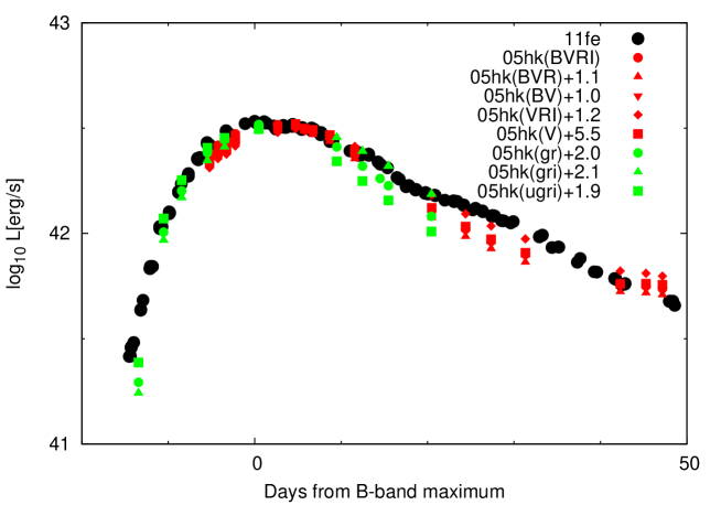
Figure 19: The bolometric light curves of SN 2005hk constructed based on the data taken with different combinations of the photometric bands. The different symbol or color denotes the luminosity estimated using the different bands. These light curves are shifted vertically with the amount indicated in the top-right portion of the panel to match with the $BVRI$ light curve around maximum light. The $BVRI$ light curve is assumed to be bolometric, which matches to The bolometric light curve of SN 2011fe with an arbitrary shift in the vertical axis (black circles).

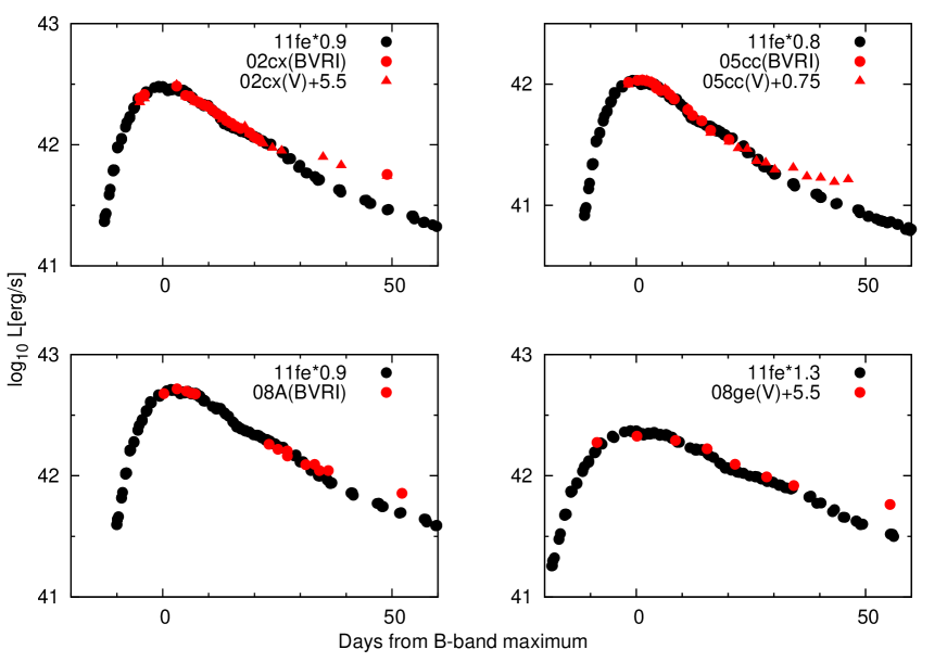
Figure 20: The bolometric light curves of SNe 2002cx (left top), 2005cc (right top), 2008A (left bottom), 2008ge (right bottom). We plot in the same manner as in Figure 19.

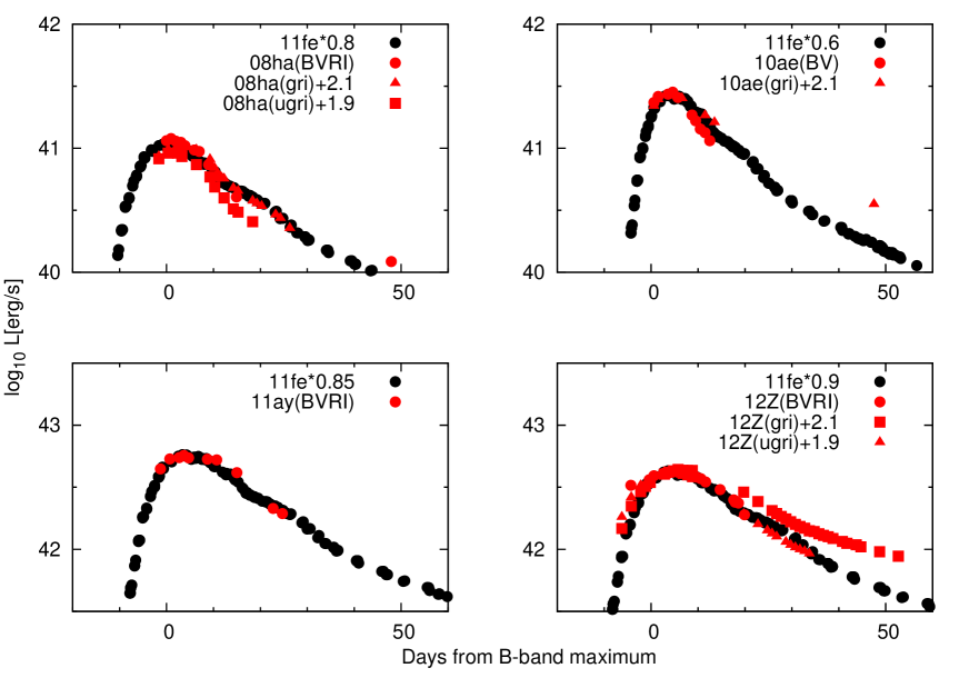
Figure 21: The bolometric light curves of SNe 2008he (left top), 2010ae (right top), 2011ay (left bottom), 2012Z (right bottom). We plot in the same manner as in Figure 19.

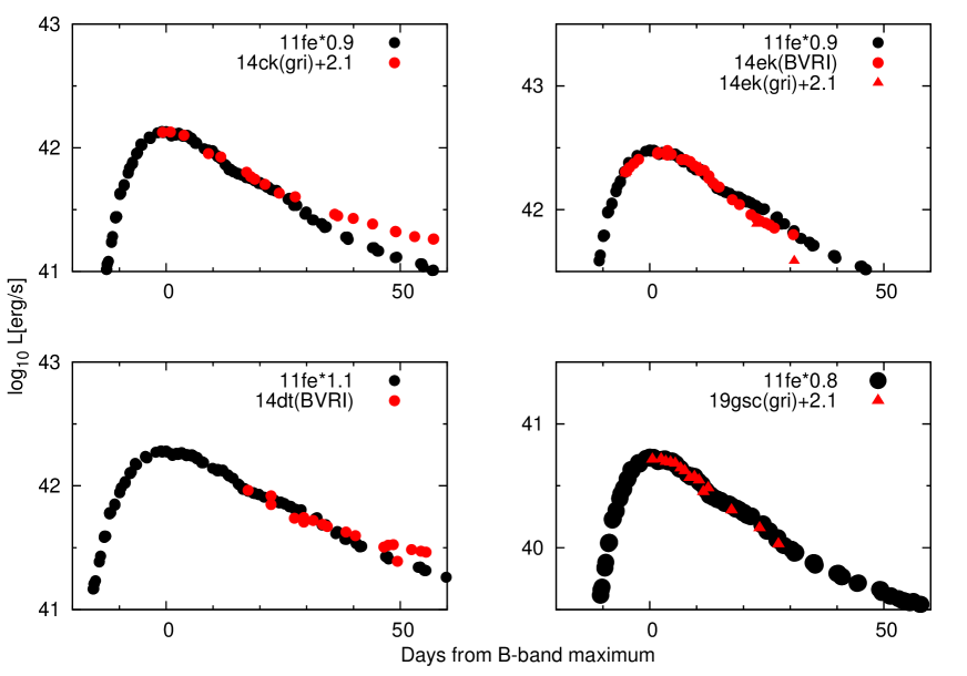
Figure 22: The bolometric light curves of SNe 2014ck (left top), 2014ek (right top), 2014dt (left bottom). We plot in the same manner as in Figure 19. The open circles of SN 2014dt is the bolometric light curve assuming that the sum of fluxes in the $BVRI$-bands occupied about 60 % of the bolometric one.

References

- Akitaya et al. (2014) Akitaya, H., et al. 2014, in Society of Photo-Optical Instrumentation Engineers (SPIE) Conference Series, Vol. 9147, Proc. SPIE, 91474O
- Arnett (1982) Arnett, W. D. 1982, ApJ, 253, 785
- Barden & Armandroff (1995) Barden, S. C., & Armandroff, T. 1995, in Society of Photo-Optical Instrumentation Engineers (SPIE) Conference Series, Vol. 2476, Fiber Optics in Astronomical Applications, ed. S. C. Barden, 56–67
- Barden et al. (1994) Barden, S. C., Armandroff, T., Muller, G., Rudeen, A. C., Lewis, J., & Groves, L. 1994, in Society of Photo-Optical Instrumentation Engineers (SPIE) Conference Series, Vol. 2198, Instrumentation in Astronomy VIII, ed. D. L. Crawford & E. R. Craine, 87–97
- Barna et al. (2021) Barna, B., et al. 2021, MNRAS, 501, 1078
- Blondin et al. (2012) Blondin, S., et al. 2012, AJ, 143, 126
- Breeveld et al. (2011) Breeveld, A. A., Landsman, W., Holland, S. T., Roming, P., Kuin, N. P. M., & Page, M. J. 2011, in American Institute of Physics Conference Series, Vol. 1358, American Institute of Physics Conference Series, ed. J. E. McEnery, J. L. Racusin, & N. Gehrels, 373–376
- Brimacombe et al. (2019) Brimacombe, J., et al. 2019, The Astronomer’s Telegram, 13004, 1
- Fink et al. (2014) Fink, M., et al. 2014, MNRAS, 438, 1762
- Foley et al. (2010) Foley, R. J., Brown, P. J., Rest, A., Challis, P. J., Kirshner, R. P., & Wood-Vasey, W. M. 2010, ApJ, 708, L61
- Foley et al. (2013) Foley, R. J., et al. 2013, ApJ, 767, 57
- Foley et al. (2009) —. 2009, AJ, 138, 376
- Foley et al. (2016) Foley, R. J., Jha, S. W., Pan, Y.-C., Zheng, W. K., Bildsten, L., Filippenko, A. V., & Kasen, D. 2016, MNRAS, 461, 433
- Foley et al. (2014) Foley, R. J., McCully, C., Jha, S. W., Bildsten, L., Fong, W.-f., Narayan, G., Rest, A., & Stritzinger, M. D. 2014, ApJ, 792, 29
- Ganeshalingam et al. (2010) Ganeshalingam, M., et al. 2010, ApJS, 190, 418
- Hayden et al. (2010) Hayden, B. T., et al. 2010, ApJ, 712, 350
- Hicken et al. (2009) Hicken, M., et al. 2009, ApJ, 700, 331
- Hicken et al. (2012) —. 2012, ApJS, 200, 12
- Hiramatsu et al. (2019) Hiramatsu, D., Arcavi, I., Burke, J., Howell, D. A., McCully, C., Pellegrino, C., & Valenti, S. 2019, Transient Name Server Classification Report, 2019-1442, 1
- Hoeflich & Khokhlov (1996) Hoeflich, P., & Khokhlov, A. 1996, ApJ, 457, 500
- Hoeflich et al. (1995) Hoeflich, P., Khokhlov, A. M., & Wheeler, J. C. 1995, ApJ, 444, 831
- Holtzman et al. (2008) Holtzman, J. A., et al. 2008, AJ, 136, 2306
- Jha et al. (2006) Jha, S., Branch, D., Chornock, R., Foley, R. J., Li, W., Swift, B. J., Casebeer, D., & Filippenko, A. V. 2006, AJ, 132, 189
- Jha (2017) Jha, S. W. 2017, Type Iax Supernovae, ed. A. W. Alsabti & P. Murdin, 375
- Jiang et al. (2020) Jiang, J.-a., et al. 2020, ApJ, 892, 25
- Jordan et al. (2012) Jordan, George C., I., Perets, H. B., Fisher, R. T., & van Rossum, D. R. 2012, ApJ, 761, L23
- Kashikawa et al. (2002) Kashikawa, N., et al. 2002, PASJ, 54, 819
- Kawabata et al. (2008) Kawabata, K. S., et al. 2008, in Proc. SPIE, Vol. 7014, Ground-based and Airborne Instrumentation for Astronomy II, 70144L
- Kawabata et al. (2018) Kawabata, M., et al. 2018, PASJ, 70, 111
- Kawabata et al. (2020) —. 2020, ApJ, 893, 143
- Kromer et al. (2013) Kromer, M., et al. 2013, MNRAS, 429, 2287
- Kromer et al. (2015) —. 2015, MNRAS, 450, 3045
- Kurita et al. (2020) Kurita, M., et al. 2020, PASJ, 72, 48
- Landolt (1992) Landolt, A. U. 1992, AJ, 104, 340
- Lennarz et al. (2012) Lennarz, D., Altmann, D., & Wiebusch, C. 2012, A&A, 538, A120
- Li et al. (2018) Li, L., et al. 2018, MNRAS, 478, 4575
- Li et al. (2003) Li, W., et al. 2003, PASP, 115, 453
- Liu et al. (2015) Liu, Z.-W., et al. 2015, MNRAS, 452, 838
- Maeda et al. (2003) Maeda, K., Mazzali, P. A., Deng, J., Nomoto, K., Yoshii, Y., Tomita, H., & Kobayashi, Y. 2003, ApJ, 593, 931
- Maeda & Terada (2016) Maeda, K., & Terada, Y. 2016, International Journal of Modern Physics D, 25, 1630024
- Magee et al. (2016) Magee, M. R., et al. 2016, A&A, 589, A89
- Matsubayashi et al. (2019) Matsubayashi, K., et al. 2019, PASJ, 71, 102
- McClelland et al. (2010) McClelland, C. M., et al. 2010, ApJ, 720, 704
- McCully et al. (2021) McCully, C., et al. 2021, arXiv e-prints, arXiv:2106.04602
- Moriya et al. (2010) Moriya, T., Tominaga, N., Tanaka, M., Nomoto, K., Sauer, D. N., Mazzali, P. A., Maeda, K., & Suzuki, T. 2010, ApJ, 719, 1445
- Nagayama et al. (2003) Nagayama, T., et al. 2003, in Society of Photo-Optical Instrumentation Engineers (SPIE) Conference Series, Vol. 4841, Proc. SPIE, ed. M. Iye & A. F. M. Moorwood, 459–464
- Narayan et al. (2011) Narayan, G., et al. 2011, ApJ, 731, L11
- Nomoto et al. (1976) Nomoto, K., Sugimoto, D., & Neo, S. 1976, Ap&SS, 39, L37
- Nugent et al. (2011) Nugent, P. E., et al. 2011, Nature, 480, 344
- Pereira et al. (2013) Pereira, R., et al. 2013, A&A, 554, A27
- Perlmutter et al. (1999) Perlmutter, S., et al. 1999, ApJ, 517, 565
- Persson et al. (1998) Persson, S. E., Murphy, D. C., Krzeminski, W., Roth, M., & Rieke, M. J. 1998, AJ, 116, 2475
- Phillips (1993) Phillips, M. M. 1993, ApJ, 413, L105
- Phillips et al. (2007) Phillips, M. M., et al. 2007, PASP, 119, 360
- Richardson et al. (2001) Richardson, D., Thomas, R. C., Casebeer, D., Blankenship, Z., Ratowt, S., Baron, E., & Branch, D. 2001, in American Astronomical Society Meeting Abstracts, Vol. 199, 84.08
- Riess et al. (1998) Riess, A. G., et al. 1998, AJ, 116, 1009
- Riess et al. (1999) —. 1999, AJ, 118, 2675
- Sahu et al. (2008) Sahu, D. K., et al. 2008, ApJ, 680, 580
- Schlafly & Finkbeiner (2011) Schlafly, E. F., & Finkbeiner, D. P. 2011, ApJ, 737, 103
- Shappee et al. (2014) Shappee, B., et al. 2014, in American Astronomical Society Meeting Abstracts, Vol. 223, American Astronomical Society Meeting Abstracts #223, 236.03
- Silverman et al. (2012) Silverman, J. M., et al. 2012, MNRAS, 425, 1789
- Singh et al. (2018) Singh, A., Srivastav, S., Kumar, B., Anupama, G. C., & Sahu, D. K. 2018, MNRAS, 480, 2475
- Srivastav et al. (2020) Srivastav, S., et al. 2020, arXiv e-prints, arXiv:2001.09722
- Stritzinger et al. (2002) Stritzinger, M., et al. 2002, AJ, 124, 2100
- Stritzinger & Leibundgut (2005) Stritzinger, M., & Leibundgut, B. 2005, A&A, 431, 423
- Stritzinger et al. (2014) Stritzinger, M. D., et al. 2014, A&A, 561, A146
- Stritzinger et al. (2015) —. 2015, A&A, 573, A2
- Szalai et al. (2015) Szalai, T., et al. 2015, MNRAS, 453, 2103
- Tomasella et al. (2016) Tomasella, L., et al. 2016, MNRAS, 459, 1018
- Valenti et al. (2009) Valenti, S., et al. 2009, Nature, 459, 674
- van Dokkum (2001) van Dokkum, P. G. 2001, PASP, 113, 1420
- van Dokkum et al. (2012) van Dokkum, P. G., Bloom, J., & Tewes, M. 2012, L.A.Cosmic: Laplacian Cosmic Ray Identification, Astrophysics Source Code Library
- Vennes et al. (2017) Vennes, S., Nemeth, P., Kawka, A., Thorstensen, J. R., Khalack, V., Ferrario, L., & Alper, E. H. 2017, Science, 357, 680
- Yamanaka et al. (2015) Yamanaka, M., et al. 2015, ApJ, 806, 191
- Yaron & Gal-Yam (2012) Yaron, O., & Gal-Yam, A. 2012, PASP, 124, 668
- Yoshida (2005) Yoshida, M. 2005, Journal of Korean Astronomical Society, 38, 117
- Zhang et al. (2016) Zhang, K., et al. 2016, ApJ, 820, 67