Spin-valley Silin modes in graphene with substrate-induced spin-orbit coupling

Abstract

In the presence of external magnetic field the Fermi-liquid state supports oscillatory spin modes known as Silin modes. We predict the existence of the generalized Silin modes in a multivalley system, monolayer graphene. A gauge- and Berry-gauge- invariant kinetic equation for a multivalley Fermi liquid is developed and applied to the case of graphene with extrinsic spin-orbit coupling (SOC). The interplay of SOC and Berry curvature allows for the excitation of generalized Silin modes in the spin and valley-staggered-spin channels via an AC electric field. The resonant contributions from these modes to the optical conductivity are calculated.

It has long been known that while spin waves in a Fermi liquid are normally overdamped [1], in the presence of a finite Zeeman field (a magnetic field acting only on particle spins) there exist well-defined, gapped spin collective modes of the Fermi-liquid state, the Silin modes [2, 3, 4, 5, 6, 7, 8]. In multi-valley materials there may be additional collective excitations of the Fermi liquid state, beyond the charge and spin modes. These additional modes are in general also diffusive in the time reversal symmetric case [9]. However, in a finite Zeeman field these modes may become oscillatory, generalizing the notion of the Silin mode. The aim of this work is to identify these combined spin-valley modes in graphene and explore ways to excite them.

We predict a set of generalized Silin modes in graphene, comprised of the spin density Silin mode as well as a new valley-staggered Silin mode, which become oscillatory in a finite in-plane magnetic field. The mode frequencies differ from each other due to the difference between the corresponding Landau Fermi-liquid constants. An effective coupling of an electromagnetic wave to the new valley-staggered modes can be achieved by engaging the spin-orbit coupling (SOC) induced by a substrate, see, e.g., [10]. Additionally, as is the case for the usual Silin mode, SOC allows the generalized Silin modes to be excited by the electric field of the wave; this results in electric dipole spin resonance (EDSR) being the dominant [11, 12, 13, 14] excitation mechanism.

We investigate the structure and frequencies of generalized Silin modes and find the corresponding resonances in the conductivity tensor. The modes differ not only by their frequency, but also by sensitivity to the polarization of the EM wave exciting them, allowing modes of different character to be selectively excited.

We consider a graphene sheet with spin-orbit coupling induced by the substrate made, e.g., of a transition metal dichalcogenide (TMD) [10]. In addition to SOC, the substrate in general also induces gaps at Dirac points in the graphene’s electronic spectrum. We assume the electron density is tuned away from the charge-neutrality point, allowing us to apply the Fermi-liquid theory. The system is subject to a static, in-plane magnetic field $\mathbf{H}_{0}$ needed for the generalized Silin modes, and an AC field $\mathbf{E}(t)$ probing them.

To describe the generalized Silin modes at long wavelength we augment the theory of a multi-valley Fermi liquid [15, 16, 9] by including the effects of SOC and of the external fields. To deduce the linear response to the probe fields, we must first obtain the energy functional with extrinsic spin-orbit coupling and applied Zeeman field.

Model. In the presence of extrinsic spin-orbit coupling, the single-particle Dirac Hamiltonian written in the valley-sub-lattice basis $(KA,KB,K^{\prime}B,-K^{\prime}A)$ takes the form

$$\hat{H}_{\mathbf{p}}=v^{\phantom{2}}_{D}\mathbf{p}\cdot\hat{\bm{\Sigma}}+\Delta\hat{\Sigma}_{z}\hat{\tau}_{z}+\lambda\hat{\tau}_{z}\hat{\sigma}_{z}+\lambda^{\phantom{2}}_{R}\mathbf{e}_{z}\cdot(\hat{\bm{\sigma}}\times\hat{\bm{\Sigma}})\,.$$ (1)

Here $\hat{\bm{\Sigma}}$, $\hat{\bm{\tau}}$, and $\hat{\bm{\sigma}}$ are the vectors of Pauli matrices in the spaces of sub-lattices ($A,B$), points $K,K^{\prime}$ in the Brillouin zone, and electron spin, respectively, and $\mathbf{e}_{z}$ is the unit vector in the $z$ (out-of-plane) direction. In the absence of SOC, the graphene spectrum is characterized by the Dirac velocity $v_{D}$ and gap $\Delta$; the valley-Zeeman ($\lambda$) and Rashba ($\lambda_{R}$) spin-orbit couplings arise from the inversion symmetry breaking by and wave function hybridization with the TMD substrate [10]. For definiteness, we take the Fermi level to be in the upper band. If the SOC couplings are small compared to the Fermi energy (as measured from charged neutrality), we may perform the projection onto the upper band perturbatively in $\lambda_{R}$ and $\lambda$, obtaining the effective single band Hamiltonian (see [17] for details)

$$\hat{H}^{+}_{\mathbf{p}}=\epsilon_{\mathbf{p}}-\frac{1}{2}\mu_{s}\mathbf{H}_{0}\cdot\hat{\bm{\sigma}}+\alpha_{R}(p)(\mathbf{p}\times\mathbf{e}_{z})\cdot\hat{\bm{\sigma}}+\Lambda(p)\hat{\sigma}_{z}\hat{\tau}_{z}$$ (2)

with $\epsilon_{\mathbf{p}}=\sqrt{v_{D}^{2}p^{2}+\Delta^{2}}$ being the massive Dirac dispersion, $\alpha_{R}(p)=v_{D}\lambda_{R}/\epsilon_{\mathbf{p}}$ the effective Rashba coupling, $\Lambda(p)=\lambda-\lambda_{R}^{2}\Delta/\epsilon_{\mathbf{p}}^{2}$ the effecive valley-Zeeman coupling, and where we have included the Zeeman energy due to external magnetic field $\mathbf{H}_{0}$ for particles with effective Bohr magneton $\mu_{s}=g_{s}e/4m_{e}c$, where $g_{s}$ is the Landé factor and $m_{e}$ is the free electron mass. A complete description of the dynamics of the projected upper band also requires the evaluation of the Berry connection, $\bm{\mathcal{\hat{A}}}$, which consists of Abelian and non-Abelian parts [18, 19]. To leading order in the Rashba term, we find $\bm{\mathcal{\hat{A}}}=\bm{\mathcal{\hat{A}}}_{0}+\bm{\mathcal{\hat{A}}}_{1}+\mathcal{O}\left(\alpha_{R}^{3}\right)$, where $\bm{\mathcal{\hat{A}}}_{0}$ is the Abelian Berry connection of gapped graphene, while the non-Abelian part is given by

$$\bm{\mathcal{\hat{A}}}_{1}=-\tilde{\alpha}_{R}(p)2\pi\nu(\epsilon_{\mathbf{p}})\lvert\Omega_{0}^{z}(p)\rvert\hat{\bm{\sigma}}_{\parallel}\hat{\tau}_{z}.$$ (3)

Here, $\boldsymbol{\Omega}=\Omega^{z}_{0}\mathbf{e}_{z}$ is the Berry curvature of gapped graphene, $\Omega_{0}^{z}(p)=\mp v_{D}^{2}\Delta/2\epsilon_{\mathbf{p}}^{3}$ with $\mp$ corresponding to the $K$ ($K^{\prime}$) point, $\nu(\epsilon)=\epsilon/2\pi v_{D}^{2}$ is the density of states of the graphene bands , and $\hat{\bm{\sigma}}_{\parallel}=\hat{\sigma}_{x}\hat{x}+\hat{\sigma}_{y}\hat{y}$. The tilde on $\tilde{\alpha}_{R}$ indicates renormalization of the effective Rashba strength which will be discussed below. The valley-Zeeman term by itself does not give rise to a non-Abelian Berry connection because it commutes with the Dirac part of the Hamiltonian.

With Eqs. 2 and 3 we are able to write a kinetic equation for the projected upper band in the collisionless limit [21]

$$\partial_{t}\hat{\rho}+\frac{1}{2}\{\bm{\nabla}\hat{\rho}\overset{\cdot}{,}\hat{\mathbf{v}}\}+\frac{1}{2}\{\bm{\mathcal{D}}\hat{\rho}\overset{\cdot}{,}\hat{\bm{F}}\}+i\left[\hat{\epsilon},\hat{\rho}\right]=0,$$ (4)

where $\hat{\rho}$ is the density matrix, $\hat{\epsilon}$ is the (matrix) quasiparticle energy functional, $\hat{\bm{F}}$ is the total force (external plus self-consistent) acting on a quasiparticle, and the Berry covariant derivative is defined as [18, 19]

$$\bm{\mathcal{D}}\hat{g}=\nabla^{(\mathbf{p})}\hat{g}-\imath[\bm{\mathcal{\hat{A}}},\hat{g}]$$ (5)

with $\nabla^{(\mathbf{p})}$ denoting the gradient in momentum space. The velocity and force appearing in Eq. 4 are governed by the quasiclassical equations of motion for the band [21, 19]. As we are working in the 2D limit, the non-Abelian Berry connection $\bm{\mathcal{A}}$ is completely in plane, while the non-abelian Berry curvature $\bm{\Omega}$ is entirely out of plane. Here, we will take take $\mathbf{E},\mathbf{H}_{0}$ to be in plane, allowing the force and velocity terms to be simply written as

$$\hat{\mathbf{v}}\approx\bm{\mathcal{D}}\hat{\epsilon},\quad\hat{\bm{F}}\approx e\bm{E}-\bm{\nabla}\hat{\epsilon}.$$ (6)

Here we have noted that in Eq. 4 $\mathbf{v}$ multiplies $\bm{\nabla}\hat{\rho}$. The latter appears in first order in $\mathbf{E}$, so within the linear response theory we can neglect terms of order $\mathbf{E}$ in $\mathbf{v}$.

The system of Eqs. 4 and 6 provides a gauge- and Berry-gauge-invariant description of the dynamics of the system. As such, it is a convenient launching point to incorporate the interplay between band topology, spin orbit coupling, and Fermi-liquid effects.

The quasiparticle energy functional is found by combining Eq. 2 with the interactions allowed by the approximate $SU(2)$ spin and $U(1)$ valley symmetries of gapped graphene [15, 16, 9]

$$\hat{\epsilon}_{\text{FL}}[\hat{\rho}_{\mathbf{p}}]=\sum_{\mathbf{p}^{\prime}}\left[f^{d}_{\mathbf{p}\mathbf{p}^{\prime}}n_{\mathbf{p}^{\prime}}+f^{s}_{\mathbf{p}\mathbf{p}^{\prime}}\mathbf{s}_{\mathbf{p}^{\prime}}\cdot\hat{\bm{\sigma}}+f^{v\parallel}_{\mathbf{p}\mathbf{p}^{\prime}}\mathbf{Y}_{\mathbf{p}^{\prime}}\cdot\hat{\bm{\tau}}_{\parallel}\right.\\ \left.+f^{vz}_{\mathbf{p}\mathbf{p}^{\prime}}Y^{z}_{\mathbf{p}^{\prime}}\hat{\tau}_{z}+f^{m\parallel}_{\mathbf{p}\mathbf{p}^{\prime}}\mathbf{M}^{i}_{\mathbf{p}^{\prime}}\cdot\hat{\bm{\sigma}}\hat{\tau}_{\parallel,i}+f^{mz}_{\mathbf{p}\mathbf{p}^{\prime}}\mathbf{M}^{z}_{\mathbf{p}^{\prime}}\cdot\hat{\bm{\sigma}}\hat{\tau}_{z}\right]\,,$$ (7)

where $\hat{{\tau}}_{\parallel,i}$ are the $\hat{\tau}_{x}$ and $\hat{\tau}_{y}$ components of $\hat{\bm{\tau}}$, and index $i$ is summed over $i=x,y$. Here we have decomposed the density matrix in terms of symmetry distinguished channels,

$$\hat{\rho}_{\mathbf{p}}=n_{\mathbf{p}}+\mathbf{s}_{\mathbf{p}}\cdot\hat{\bm{\sigma}}+\mathbf{Y}_{\mathbf{p}}\cdot\hat{\bm{\tau}}+\mathbf{M}_{\mathbf{p}}^{i}\cdot\hat{\bm{\sigma}}\hat{\tau}_{i},$$ (8)

and $f^{\mu}_{\mathbf{p}\mathbf{p^{\prime}}}$ are the Landau-Fermi liquid interaction functions associated with the channel. The collective variables in Eq. 8 are the densities of: charge $n$, spin $\mathbf{s}$, valley pseudo-spin $\mathbf{Y}$, and spin-triplet valley pseudo-spin $\mathbf{M}^{i}$.

Before considering the collective modes, we must identify the equilibrium density matrix. The equilibrium occupations in the spin and valley-spin channels are due to the presence of the external Zeeman field and Rashba coupling for the former, and valley-Zeeman coupling for the latter. We consider the case where the thermal, spin-orbit, and magnetic energy scales are small compared to the Fermi energy with respect to the band edge, $T,\mu_{s}H_{0},\lambda,\lambda_{R}\ll E_{F}-\Delta$. In direct analogy with the standard computation of the spin magnetic moment of the Fermi liquid [22, 23], the equilibrium density matrix is given by Eq. 8 with [17]

$$\begin{gathered}n_{\text{eq},\mathbf{p}}=n_{F}(\tilde{\epsilon}_{\mathbf{p}}),\quad Y_{\text{eq},\mathbf{p}}=0\\ \mathbf{s}_{\text{eq},\mathbf{p}}=-\frac{\partial n_{F}}{\partial\epsilon}\left(\frac{1}{2}\tilde{\mu}_{s}\mathbf{H}_{0}-\tilde{\alpha}_{R}(p)\mathbf{p}\times\mathbf{e}_{z}\right),\\ \mathbf{M}^{i}_{\text{eq},\mathbf{p}}=\frac{\partial n_{F}}{\partial\epsilon}\tilde{\Lambda}(p)\mathbf{e}_{z}\delta_{iz}.\end{gathered}$$ (9)

Here, $n_{F}$ is the Fermi function of the local excitation energy in the absence of SOC and magnetic field given by $\tilde{\epsilon}_{\mathbf{p}}=\epsilon_{\mathbf{p}}+\sum_{\mathbf{p}^{\prime}}f^{d}_{\mathbf{p}\mathbf{p}^{\prime}}n_{F}(\tilde{\epsilon}_{\mathbf{p}^{\prime}})$ , and $\epsilon_{\mathbf{p}}$ is defined in Eq. 2. $\tilde{\mu}_{s}$, $\tilde{\alpha}(p)$, and $\tilde{\Lambda}(p)$ are, respectively, the renormalized by interaction effective spin magnetic moment, Rashba SOC strength [25], and valley-Zeeman SOC strength:

$$\tilde{\mu}_{s}=\frac{\mu_{s}}{1+F_{0}^{s}},\ \tilde{\alpha}_{R}(p)=\frac{\alpha_{R}(p)}{1+F_{1}^{s}},\ \tilde{\Lambda}(p)=\frac{\Lambda(p)}{1+F^{mz}_{0}}.$$ (10)

The Landau Fermi-liquid parameters in Eq. 10 are

$$F^{\mu}_{l}=G_{s}G_{v}\nu_{F}\int\frac{d\phi}{2\pi}\frac{d\phi^{\prime}}{2\pi}f^{\mu}(\mathbf{p}_{F},\mathbf{p}^{\prime}_{F})e^{-il(\phi-\phi^{\prime})},$$ (11)

where $\phi,\phi^{\prime}$ are the azimuths of the respective momenta on the Fermi circles in valleys $K$ and $K^{\prime}$ and $\mu=d,s,{v\!\!\parallel,}\,vz,m\!\!\parallel,mz$; also, $\nu_{F}$ is the density of states at the Fermi surface, and $G_{s}$ and $G_{v}$ are the spin and valley degeneracy, respectively.

Following the above considerations, we write the equilibrium energy $\hat{\epsilon}_{\text{eq}}\equiv\hat{\epsilon}[\hat{\rho}_{\text{eq}}]$ as

$$\hat{\epsilon}_{\text{eq}}=\tilde{\epsilon}_{\mathbf{p}}-\left(\frac{1}{2}\tilde{\mu}_{s}\mathbf{H}_{0}-\tilde{\alpha}_{R}(p)(\mathbf{p}\times\mathbf{e}_{z})\right)\cdot\hat{\bm{\sigma}}+\tilde{\Lambda}\hat{\sigma}_{z}\hat{\tau}_{z}.$$ (12)

Linear response. To find the EDSR response of the system, we need to keep only linear-order terms in the electric field. We thus linearize the kinetic equation (4) in the deviation from equilibrium $\hat{\rho}\equiv\hat{\rho}_{\text{eq}}+\delta\hat{\rho}$:

$$\partial_{t}\delta\hat{\rho}+\frac{1}{2}\nabla\cdot\left[\{\hat{\mathbf{v}},\delta\hat{\rho}\}-\{\delta\hat{\epsilon}{,}\bm{\mathcal{D}}\hat{\rho}_{\text{eq}}\}\right]+i[\hat{\epsilon}_{\text{eq}},\delta\hat{\bar{\rho}}]\\ =-e\mathbf{E}\cdot\bm{\mathcal{D}}\hat{\rho}_{\text{eq}},$$ (13)

where we have defined the first-order correction to the quasiparticle energy from fluctuations in terms of the the Fermi-liquid interactions $\delta\hat{\epsilon}=\hat{\epsilon}_{\text{FL}}[\delta\hat{\rho}]$ (cf. Eq. (7)), and the local deviation from equilibrium $\delta\hat{\bar{\rho}}\equiv\delta\hat{\rho}-(\partial n_{F}/\partial\epsilon)\delta\hat{\epsilon}$.

From Eq. 13 we obtain the conductivity as follows. First, by taking the trace of Eq. 13 and integrating it over momentum, we find the continuity equation,

$$e\sum_{\mathbf{p}}\operatorname{tr}\partial_{t}\delta\hat{\rho}+\bm{\nabla}\cdot e\sum_{\mathbf{p}}\operatorname{tr}\left(\hat{\mathbf{v}}_{\mathbf{p}}\delta\hat{\rho}-\delta\hat{\epsilon}\bm{\mathcal{D}}\hat{\rho}_{\text{eq}}\right)=0\,,$$ (14)

which allows us to identify the longitudinal charge current as

$$\mathbf{j}=e\sum_{\mathbf{p}}\operatorname{tr}\left(\hat{\mathbf{v}}_{\mathbf{p}}\delta\hat{\rho}-\delta\hat{\epsilon}\bm{\mathcal{D}}\hat{\rho}_{\text{eq}}\right).$$ (15)

Using the equilibrium energy c12 and density matrix of Eq. 9 allows us to write the spin contribution to the longitudinal current (to order $\alpha_{R}^{2}$ and lowest order in $\lambda/\omega_{s}$). Expanding the dynamic variables into the angular harmonics on the Fermi surface,

$$\begin{gathered}\delta\mathbf{s}_{\mathbf{p}}=-\frac{\partial n_{F}}{\partial\epsilon}\sum_{l}\delta\tilde{\mathbf{s}}_{l}e^{il\phi},\\ \delta\mathbf{M}^{z}_{\mathbf{p}}=-\frac{\partial n_{F}}{\partial\epsilon}\sum_{l}\delta\widetilde{\mathbf{M}}^{z}_{l}e^{il\phi},\end{gathered}$$ (16)

we write the current as

$$\mathbf{j}_{\text{res}}=-eG_{s}G_{v}\nu_{F}\tilde{\alpha}_{R}\left[\left(\frac{1}{2}\zeta+2\pi\nu_{F}\lvert\Omega_{0}^{z}\rvert\frac{2\lambda}{\gamma_{0}}\right)\delta\tilde{\mathbf{s}}_{0}\times\mathbf{e}_{z}\right.\\ \left.+\frac{1}{2}\left(1+F_{2}^{s}-\frac{1}{2}\zeta\right)\sum_{\pm}\pm i\left(\mathbf{e}_{R/L}\cdot\delta\tilde{\mathbf{s}}_{\pm 2}\right)\mathbf{e}_{R/L}\right]\\ +2\pi eG_{s}G_{v}\nu_{F}^{2}\lvert\Omega_{0}^{z}\rvert\tilde{\alpha}_{R}\left[\frac{1+F_{0}^{mz}}{1+F_{0}^{s}}\lvert\mu_{s}\mathbf{H}_{0}\rvert\delta\widetilde{M}^{z}_{0}\mathbf{e}_{y}\right.\\ +\left.\alpha_{R}p_{F}\left(\frac{1+F_{1}^{s}}{1+F_{0}^{mz}}+\frac{1}{2}\gamma_{1}\right)\sum_{\pm}\delta\widetilde{M}^{z}_{\pm 1}{\mathbf{e}_{R/L}}\right],$$ (17)

where $\mathbf{e}_{R/L}=\mathbf{e}_{x}\pm i\mathbf{e}_{y}$ and

$$\zeta\equiv 1+\frac{E_{F}-\sqrt{E_{F}^{2}-\Delta^{2}}}{E_{F}},\quad\gamma_{l}=\frac{1+F_{l}^{mz}}{1+F_{l}^{s}}.$$ (18)

Note that the presence of $\Omega_{0}^{z}$ in Eq. 17 indicates the important role of the Berry curvature in driving the valley-staggered modes (see also Fig. 1).

With an expression for the current in terms of $\delta\hat{\rho}$ we can solve the homogeneous $\mathbf{q}\to 0$ limit of Eq. 13 for $\delta\hat{\rho}$, obtaining a linear relationship between $\mathbf{j}$ and $\mathbf{E}$, and thus read off the dissipative part of the optical conductivity tensor.

In the absence of SOC and driving, the homogeneous limit of Eq. 13 is simply

$$\partial_{t}\delta\hat{\rho}+i[\hat{\epsilon}_{\text{eq}},\delta\hat{\bar{\rho}}]=0.$$ (19)

In the spin and valley-spin sectors, this gives the equations 

$$\begin{gathered}\partial_{t}\delta\tilde{\mathbf{s}}_{l}-\omega_{sl}\mathbf{e}_{x}\times\delta\tilde{\mathbf{s}}_{l}=0,\quad\omega_{sl}=\frac{1+F_{l}^{s}}{1+F_{0}^{s}}\lvert\mu_{s}H_{0}\rvert,\\ \partial_{t}\delta\widetilde{\mathbf{M}}^{z}_{l}-\omega_{ml}\mathbf{e}_{x}\times\delta\widetilde{\mathbf{M}}^{z}_{l}=0,\quad\omega_{ml}=\gamma_{l}\omega_{sl}.\end{gathered}$$ (20)

Here $\delta\tilde{\mathbf{s}}$ corresponds to long wave-length spin-density modulations, while $\delta\widetilde{\mathbf{M}}^{z}$ describes spin-density modulations on length scale $|\bm{K}-\bm{K}^{\prime}|^{-1}$ corresponding to the separation between valleys in the Brillouin zone. As in the case of the conventional Silin mode [2], the mode frequencies are renormalized away from the Zeeman frequency by the Fermi-liquid parameters, with the exception of the $l=0$ mode frequency, which is protected by $SU(2)$ symmetry (see Ref. 17 for how this is modified by valley-Zeeman SOC).

Conductivity resonances. Without SOC, the resonant finite frequency modes are not excited by an external electric field. However, upon introduction of the Rashba coupling, three modes may be resonantly excited, namely, the $l=0$ spin and valley-staggered spin modes, and the $l=\pm 2$ spin mode.

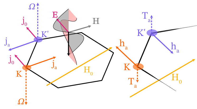
Figure 1: (Color online) Left: Electron dipole spin resonance driven by an electromagnetic wave. The regular, $\mathbf{j}_{0}\propto\mathbf{E}$, and anomalous, $\mathbf{j}_{a}\propto\bm{\Omega}\times\mathbf{E}$, currents at the $K$ (orange) and $K^{\prime}$ (purple) points in the Brillouin zone, induced by the electric field $\mathbf{E}$ of the incident electromagnetic wave. Here, $\boldsymbol{\Omega}$ is the valley-staggered Berry curvature. Right: Anomalous fields and torques. Spins are initially polarized along the Zeeman field $\mathbf{H}_{0}$. The anomalous current-induced effective Rashba fields, $\mathbf{h}_{a}\propto\alpha_{R}\mathbf{e}_{z}\times\mathbf{j}_{a}$, produce valley-specific torques $\mathbf{T}_{a}\propto\mathbf{H}_{0}\times\mathbf{h}_{a}$, thus exciting the valley-staggered spin mode with an intensity proportional to $|\mathbf{E}\times\mathbf{H}|$.

The mechanism of driving can be understood as follows. Initially, all particle spins are polarized along the external Zeeman field, which we take to be along the $\mathbf{e}_{x}$ axis. Upon application of an external field $\mathbf{E}(t)$ the particle spins feel an effective magnetic field due to the Rashba term $\mathbf{h}\propto\mathbf{e}_{z}\times\mathbf{j}$ [19, 28] and therefore a spin torque [29, 30], $\mathbf{T}\propto\mathbf{e}_{x}\times\mathbf{h}=\mathbf{e}_{z}j_{x}.$ The $x$ component of the current $j_{x}$ is composed of regular and anomalous pieces, shown in the left of Fig. 1,

$$j_{x}(\omega)=-\frac{e^{2}NE_{x}}{i\omega m^{*}}-e^{2}N\Omega_{0}^{z}E_{y},$$ (21)

where $N$ is the number density, $m^{*}=p_{F}/v_{F}$ and $v_{F}=\epsilon^{\prime}_{\mathbf{p}}|_{p=p_{F}}$. The first of these terms creates identical torques in both valleys, while the second one, being proportional to the Berry curvature, yields valley-staggered torques depicted in the right of Fig. 1. Thus, the component of $\mathbf{E}$ along $\mathbf{H}_{0}$ causes a valley-uniform torque on the spin, exciting the spin mode, $\delta\tilde{\mathbf{s}}$, while the component of $\mathbf{E}$ transverse to $\mathbf{H}_{0}$ causes a valley-staggered torque, and thus excites the valley-staggered spin mode, $\delta\widetilde{\mathbf{M}}^{z}$. Because the charge-to-spin conversion in both cases is proportional to the Rashba coupling, this leads to contributions to the conductivity proportional to $\alpha_{R}^{2}$. Furthermore, the $\delta\tilde{\mathbf{s}}_{0}$ mode contributes to $\sigma^{xx}$ while the $\delta\widetilde{\mathbf{M}}^{z}_{0}$ mode contributes to $\sigma^{yy}$.

In the interacting case, the basic physical picture remains the same, but the quantities involved are renormalized. The resonant contributions to the dissipative part of the conductivity can be written as (see Ref. 17)

$$\operatorname{Re}\sigma_{1}^{ii}= \frac{1}{2}\pi e^{2}G_{s}G_{v}\nu_{F}\tilde{\alpha}^{2}_{R}W_{1}^{ii}A_{m1}(\omega^{2}),$$ (22)

$$\operatorname{Re}\sigma_{0}^{ii}= \frac{1}{2}\pi e^{2}G_{s}G_{v}\nu_{F}\tilde{\alpha}^{2}_{R}W_{0}^{ii}A_{s0}(\omega^{2}),$$

$$\operatorname{Re}\sigma_{2}= \frac{1}{2}\pi e^{2}G_{s}G_{v}\nu_{F}\tilde{\alpha}^{2}_{R}W_{2}A_{s2}(\omega^{2})$$

where $A_{\mu l}(\omega^{2})\equiv\omega_{\mu l}\delta(\omega^{2}-\omega_{\mu l}^{2})$ is the spectral function for the relevant mode and $W^{ii}_{l}$ is a dimensionless peak weight ($i=x,y$). Here the lack of indices on $\sigma_{2}$ indicates that the $l=2$ contribution is isotropic, $\sigma_{2}^{xx}=\sigma_{2}^{yy}=\sigma_{2}$, and it is understood that the total conductivity is the sum of the three lines in Eq. 22. Solving Eq. 13 in the homogeneous limit and substituting the result into Eq. 17 we find, to order $\alpha_{R}^{2}$ and without the valley-Zeeman term,

$$\begin{gathered}\lim_{\lambda\to 0}W_{1}^{ii}=0,\;\lim_{\lambda\to 0}W_{0}^{xx}=\zeta\frac{\omega_{s1}}{2\omega_{s0}},\\ \lim_{\lambda\to 0}W^{yy}_{0}=\left(2\pi\nu_{F}\lvert\Omega_{0}^{z}\rvert\right)^{2}\frac{\omega_{m0}^{2}}{1+F_{0}^{mz}},\\ \lim_{\lambda\to 0}W_{2}=2\left(1+F_{2}^{s}-\frac{1}{2}\zeta\right)\left(1-\frac{\omega_{s1}}{2\omega_{s2}}\right).\end{gathered}$$ (23)

Here we explicitly see that the contribution from the $l=0$ modes has the strong anisotropy discussed above, while the $l=2$ contribution is isotropic.

Experiment shows that valley-Zeeman coupling is generally also present [31, 32, 33]. The inclusion of the valley-Zeeman coupling leads to a modification of the weights in Eq. 23. Additionally, the valley-Zeeman term allows to excite the valley-staggered spin mode in the $l=1$ channel with frequency $\omega_{m1}$. To lowest non-trivial order in the valley-Zeeman coupling $\lambda$, the weights in Eq. 22 are modified to

$$W^{xx}_{1}= 2\tilde{\lambda}(1+F_{1}^{s})2\pi\nu_{F}\lvert\Omega_{0}^{z}\rvert$$ (24)

$$\times\left(1+\frac{1}{2}\gamma_{1}^{-1}\frac{1+F_{1}^{s}}{1+F_{0}^{mz}}\right)(1-\gamma_{1}),$$

$$W^{yy}_{1}= 2\tilde{\lambda}(1+F_{1}^{s})2\pi\nu_{F}\lvert\Omega_{0}^{z}\rvert,$$

$$\times\left[\frac{\omega_{s1}-\omega_{m1}}{\omega_{m0}-\omega_{m1}}+(1-\gamma_{1})\left(1+\frac{1}{2}\gamma_{1}^{-1}\frac{1+F_{1}^{s}}{1+F_{0}^{mz}}\right)\right]$$

$$W^{xx}_{0}= \zeta\frac{\omega_{1s}}{2\omega_{s}}+2\tilde{\lambda}(2\pi\nu_{F}\lvert\Omega_{0}^{z}\rvert)\left(1+F_{1}^{s}-\zeta\right)$$

$$W^{yy}_{0}= 2\pi\nu_{F}\lvert\Omega^{z}_{0}\rvert\Bigg{\{}2\pi\nu_{F}\lvert\Omega_{0}^{z}\rvert\frac{\omega^{2}_{m0}}{1+F_{0}^{mz}}$$

$$+2\tilde{\lambda}\left[(1+F_{1}^{mz})\frac{\omega_{s1}-\omega_{m0}}{\omega_{m0}-\omega_{m1}}-\frac{1}{1+F_{0}^{mz}}\zeta\right]\Bigg{\}};$$

while $W_{2}$ remains unchanged. Note that there are two qualitatively different contributions to $W_{1}$. One gives $W_{1}^{xx}$ and the second term in $W_{2}^{yy}$ (which are identical) and comes from coupling of the $l=1$ $\delta\widetilde{\mathbf{M}}^{z}$ mode to the $l=1$ spin zero-mode $\delta\tilde{\mathbf{s}}_{l=\pm 1}$, with magnetization parallel to $\mathbf{H}_{0}$, via the valley-Zeeman SOC. The other term, corresponding to the first term of $W_{1}^{yy}$ arises from conversion of the $l=0$ $\delta\widetilde{\mathbf{M}}^{z}$ mode into the $l=1$ mode via the Rashba SOC, which carries angular momentum $1$. Both of these processes can only occur in the presence of interactions – specifically when $F^{mz}_{1}\neq F^{s}_{1}$ and $F^{mz}_{1}\neq F^{mz}_{0}$ respectively  – and arise due to the different effective magnetic moments for Zeeman vs valley-Zeeman fields.

Discussion. It should be noted that these modes may be driven as well by an AC magnetic field. Indeed, as discussed above, EDSR may be interpreted as being due to an effective Zeeman field created by the external electric field and Rashba coupling [11, 14]. The relative strength of EDSR driving compared to driving by an AC magnetic field is of the order of the ratio of atomic energy scale to driving frequency $E_{\text{at}}/\omega\gg 1$ , confirming the leading role of SOC in driving the modes [12, 25].

The visibility of the generalized Silin modes in the optical conductivity will be determined by the broadening of the Silin mode peaks, as well as by the extent of the Drude peak tail. In principle, this depends on two different relaxation times, the momentum relaxation time $\tau$ and spin relaxation time $\tau_{s}$. We may approximate the effect of the spin relaxation on the Silin mode peaks by broadening the $\delta$-function peak to a Lorentizan of width $\tau_{s}^{-1}$. Doing so, one may compute the ratio of the absorption peak height to the background Drude conductivity. Writing the latter as $\sigma_{D}(\omega)=e^{2}G_{s}G_{v}\nu_{F}D/(1-i\omega\tau)$ with diffusion constant $D=v_{F}^{2}\tau(1+F_{0}^{d})/2,$ we can express the ratio of the resonant to Drude parts of the conductivity as

$$\frac{\operatorname{Re}\sigma_{\text{res}}(\omega=\omega_{i})}{\operatorname{Re}\sigma_{D}(\omega=\omega_{i})}\approx\frac{1+(\omega_{i}\tau)^{2}}{2}\frac{\tilde{\alpha}^{2}_{R}}{v_{F}^{2}}\frac{\tau_{s}}{\tau}\frac{W_{i}}{1+F_{0}^{d}}\,,$$ (25)

where $W_{i}$ is the weight of the $\delta$-function for a resonant mode, cf. Eqs. 24 and 22. The ratio $\tau_{s}/\tau_{p}$, extracted from weak anti-localization measurements in graphene on TMD, varies between different studies [36, 10, 31, 32, 33]. To be specific, we take $\tau_{s}\sim\tau\sim$1\text{\,}\mathrm{p}\mathrm{s}$$ [32]. Then the resonant contribution is enhanced by applying a strong in-plane magnetic field ($H_{0}>$10\text{\,}\mathrm{T}$$) and also by choosing a material with larger $\tilde{\alpha}_{R}$. From the beatings of Shubnikov-de Haas oscillations in bilayer graphene on WSe₂ one extracts $\lambda_{R}=10-15$ meV [10]; then $\tilde{\alpha}_{R}/v_{F}\sim\lambda_{R}/E_{F}\sim 0.1$.

To conclude, in this work we have shown that in the presence of an external magnetic field the normally diffusive spin-valley modes of graphene evolve into well-defined oscillatory modes with frequency set by the Larmor frequency, and Landau-Fermi liquid parameters, see Eq. (20). The modes are a generalization of the Silin mode to multi-valley materials. They can be probed via electric dipole spin resonance (EDSR) in the presence of extrinsic spin-orbit coupling. Furthermore, certain modes may be selectively excited by changing the polarization of applied $E$ fields, leading to anisotropy of the optical conductivity, see Eqs. (22)-(24).

A Evaluation of the equilibrium density matrix

We consider the case where the thermal, spin-orbit, and magnetic energy scales are small compared to the Fermi energy with respect to the band edge, i.e., $T,\mu_{s}H_{0},\lambda,\lambda_{R}\ll E_{F}-\Delta$. The equilibrium components of the quasiparticle energy functional in the spin and valley-spin channels are then obtained to lowest order in SOC and Zeeman field from the self-consistent equations

$$\begin{gathered}\delta\varepsilon^{s}_{\mathbf{p}}=-\frac{1}{2}\mu_{s}\mathbf{H}_{0}+\alpha_{R}(p)\mathbf{p}\times\mathbf{e}_{z}+\sum_{\mathbf{p^{\prime}}}f^{s}_{\mathbf{p}\mathbf{p^{\prime}}}\frac{\partial n_{F}}{\partial\varepsilon}\delta\varepsilon^{s}_{\mathbf{p^{\prime}}}\,,\\ \delta\varepsilon^{mz}_{\mathbf{p}}=\Lambda(p)+\sum_{\mathbf{p^{\prime}}}f^{mz}_{\mathbf{p}\mathbf{p^{\prime}}}\frac{\partial n_{F}}{\partial\varepsilon}\delta\varepsilon^{mz}_{\mathbf{p^{\prime}}},\end{gathered}$$ (S1)

in direct analogy with the standard computation of the spin magnetic moment of the Fermi liquid [22, 23]. To same order in SOC and the Zeeman field, the equilibrium density matrix can be obtained as linear response to new terms in the energy functional

$$\hat{\rho}_{\text{eq}}\approx n_{F}(\tilde{\epsilon})+\frac{\partial n_{F}}{\partial\epsilon}\left[-\left(\frac{1}{2}\mu_{s}\mathbf{H}_{0}-\alpha_{R}(p)\mathbf{p}\times\mathbf{e}_{z}-\sum_{\mathbf{p}^{\prime}}f^{s}_{\mathbf{p}\mathbf{p}^{\prime}}\mathbf{s}_{\text{eq},\mathbf{p}^{\prime}}\right)\cdot\bm{\sigma}+\left(\Lambda\mathbf{e}_{z}\delta_{i3}+\sum_{\mathbf{p}^{\prime}}f^{mi}_{\mathbf{p}\mathbf{p}^{\prime}}\mathbf{M}^{i}_{\text{eq},\mathbf{p}^{\prime}}\right)\cdot\bm{\sigma}\tau_{i}\right].$$ (S2)

This motivates the parametrization

$$\mathbf{s}_{\text{eq}}=-\frac{\partial n}{\partial\epsilon}\left(\mathbf{m}-l\mathbf{p}\times\mathbf{e}_{z}\right),\qquad\mathbf{M}^{i}_{\text{eq}}=\frac{\partial n}{\partial\epsilon}L\mathbf{e}_{z}\delta_{i3}.$$ (S3)

Plugging Eq. S3 into Eq. S2 and using the fact that, at low $T$, the derivative of the Fermi function restricts momenta to the Fermi surface, we obtain the equations

$$\mathbf{m}-l\hat{p}\times\mathbf{e}_{z}=\frac{1}{2}\mu_{s}\mathbf{H}_{0}-F_{0}^{s}\mathbf{m}-\alpha_{R}(p)\mathbf{p}\times\mathbf{e}_{z}+lF_{1}^{s}\mathbf{p}\times\mathbf{e}_{z},\qquad L=\Lambda-F_{0}^{mz}L.$$ (S4)

These may readily be solved for

$$\mathbf{m}=\frac{1}{2}\frac{\mu_{s}\mathbf{H}_{0}}{1+F_{0}^{s}},\qquad l(p)=\frac{\alpha_{R}(p)}{1+F_{1}^{s}},\qquad L=\frac{\Lambda}{1+F^{mz}_{0}},$$ (S5)

Plugging these solutions back into $\hat{\epsilon}_{0}$ leads to Eq. 12 with the renormalized constants

$$\tilde{\mu}_{s}=\mu_{s}\frac{1}{1+F_{0}^{s}},\qquad\tilde{\alpha}_{R}(p)=\frac{\alpha_{R}(p)}{1+F_{1}^{s}}=l(p),\qquad\tilde{\lambda}=\frac{\lambda}{1+F^{mz}_{0}}=L,$$ (S6)

as they appear in the main text.

B Projection of the Hamiltonian onto the upper band

In this section, we derive the projected Hamiltonian up to order $\lambda_{R}^{2}$, employing the Schrieffer-Wolff transformation. We start with

$$\hat{H}=\hat{H}_{D}+\hat{H}_{VR},\quad\hat{H}_{D}=\mathbf{d}\cdot\bm{\Sigma},\quad\hat{H}_{VR}=\lambda_{R}\mathbf{e}_{z}\times\bm{\sigma}\cdot\bm{\Sigma}$$ (S7)

with

$$\mathbf{d}=(v_{D}p_{x},v_{D}p_{y},\Delta\hat{\tau}_{z})$$ (S8)

and $\epsilon\equiv|\mathbf{d}|$, $\mathbf{n}\equiv\mathbf{d}/\epsilon$. It is safe to neglect the valley-Zeeman term here as it commutes with $\hat{H}$. We define the projectors on the upper/lower bands of $\hat{H}_{D}$ in Eq. S7 as

$$\hat{P}_{b}=\frac{1}{2}\left(1+b\mathbf{n}\cdot\bm{\Sigma}\right),$$ (S9)

and the Hamiltonians

$$\hat{H}_{R}=\sum_{b}\hat{P}_{b}\hat{H}_{VR}\hat{P}_{b},\quad\hat{H}_{1}=\sum_{b}\hat{P}_{b}\hat{H}_{VR}\hat{P}_{-b}$$ (S10)

describing, respectively, the block-diagonal and block-off-diagonal components of the Rashba term. The “unperturbed” block-diagonal Hamiltonian is thus given by

$$\hat{H}_{0}=\hat{H}_{D}+\hat{H}_{R}=\sum_{b}b\hat{P}_{b}\left(\epsilon+\alpha_{R}(p)\mathbf{e}_{z}\times\hat{\bm{\sigma}}\cdot\mathbf{p}\right),\quad\alpha_{R}=\frac{v_{D}\lambda_{R}}{\epsilon}.$$ (S11)

The total Hamiltonian is $\hat{H}=\hat{H}_{0}+\hat{H}_{1}$, where $\hat{H}_{1}$ is the block-off-diagonal part. Explicitly

$$\hat{H}_{1}=\hat{H}_{VR}-\hat{H}_{R}=\lambda_{R}\mathbf{e}_{z}\times\hat{\bm{\sigma}}\cdot\left(\hat{\bm{\Sigma}}-\sum_{b}b\mathbf{n}\hat{P}_{b}\right).$$ (S12)

B.1 Canonical Transformation

We now consider a transformation

$$\hat{U}=e^{\hat{T}},\quad\hat{T}^{\dagger}=-\hat{T},\quad\hat{P}_{b}\hat{T}\hat{P}_{b}=0.$$ (S13)

Applying the transformation Eq. S13 to Eq. S7 gives us a transformed Hamiltonian

$$\hat{H}^{\prime}=\hat{U}\hat{H}\hat{U}^{\dagger}=\hat{U}\hat{H}_{0}\hat{U}^{\dagger}+\hat{U}\hat{H}_{1}\hat{U}^{\dagger}.$$ (S14)

Making use of the Baker-Campbell-Hausdorff relation, we expand $\hat{H}^{\prime}$ to second order in $\hat{T}$

$$\hat{H}^{\prime}\approx\hat{H}_{0}+\hat{H}_{1}+[\hat{T},\hat{H}_{0}]+[\hat{T},\hat{H}_{1}]+\frac{1}{2}[\hat{T},[\hat{T},\hat{H}_{0}]]+\cdots$$ (S15)

The Schrieffer-Wolff transformation is effected by requiring that

$$[\hat{T},\hat{H}_{0}]=-\hat{H}_{1}+\mathcal{O}(\lambda_{R}^{3}).$$ (S16)

Then to order $\lambda_{R}^{2}$, $\hat{H}^{\prime}$ becomes block-diagonal:

$$\hat{H}^{\prime}\approx\hat{H}_{0}+\frac{1}{2}[\hat{T}_{1},\hat{H}_{1}]+\mathcal{O}(\lambda_{R}^{3}).$$ (S17)

Indeed, $\hat{T}$ can be always be chosen off-diagonal, while $\hat{H}_{1}$ is off-diagonal by construction, thus the product of $\hat{T}$ and $\hat{H}_{1}$ is diagonal. Working at this order, it is straightforward to see that if we choose $\hat{T}$ to be

$$\hat{T}=\sum_{b}b\hat{P}_{b}\frac{\hat{H}_{1}}{2\epsilon}\hat{P}_{-b}+\mathcal{O}(\lambda_{R}^{3}),$$ (S18)

then Eq. S16 is indeed satisfied. The second-order correction to the Hamiltonian can be read off from Eqs. S15 and S16 as

$$\hat{H}_{2}=\frac{1}{2}[\hat{T},\hat{H}_{1}].$$ (S19)

In particular, we are interested in the projection onto the upper band

$$\hat{H}_{2}^{+}\hat{P}_{+}\equiv\hat{P}_{+}\hat{H}_{2}\hat{P}_{+}.$$ (S20)

Noting that

$$\hat{P}_{+}\hat{T}=\frac{1}{2\epsilon}\hat{P}_{+}\hat{H}_{1},\quad\hat{T}\hat{P}_{+}=-\frac{1}{2\epsilon}\hat{H}_{1}\hat{P}_{+}$$ (S21)

we have

$$\hat{H}_{2}^{+}\hat{P}_{+}=\frac{1}{2\epsilon}\hat{P}_{+}\hat{H}^{2}_{2}\hat{P}_{+}=\frac{\lambda_{R}^{2}}{2\epsilon}\hat{P}_{+}{\left(\mathbf{e}_{z}\times\hat{\bm{\sigma}}\cdot\left[\hat{\bm{\Sigma}}-\sum_{b}b\mathbf{n}\right]\right)}^{2}\hat{P}_{+}=\frac{\lambda_{R}^{2}}{2\epsilon}\hat{P}_{+}{\left(\mathbf{e}_{z}\times\hat{\bm{\sigma}}\cdot\left[\hat{\bm{\Sigma}}-\mathbf{n}\right]\right)}^{2}\hat{P}_{+}\\ =\frac{\lambda_{R}^{2}}{2\epsilon}\hat{P}_{+}\mathbf{e}_{z}\times\hat{\bm{\sigma}}\cdot\hat{\bm{\Sigma}}\left(\mathbf{e}_{z}\times\hat{\bm{\sigma}}\cdot\left[\hat{\bm{\Sigma}}-\mathbf{n}\right]\right)\hat{P}_{+}=\frac{\lambda_{R}^{2}}{2\epsilon}\hat{P}_{+}\left[{\left(\mathbf{e}_{z}\times\hat{\bm{\sigma}}\cdot\hat{\bm{\Sigma}}\right)}^{2}-{\left(\mathbf{e}_{z}\times\hat{\bm{\sigma}}\cdot\mathbf{n}\right)}^{2}\right]\hat{P}_{+}\\ =\frac{\lambda_{R}^{2}}{2\epsilon}\left[\hat{P}_{+}{\left(\mathbf{e}_{z}\times\hat{\bm{\sigma}}\cdot\hat{\bm{\Sigma}}\right)}^{2}\hat{P}_{+}-\frac{v_{D}^{2}p^{2}}{\epsilon^{2}}\hat{P}_{+}\right].$$ (S22)

Evaluating

$${\left(\mathbf{e}_{z}\times\hat{\bm{\sigma}}\cdot\hat{\bm{\Sigma}}\right)}^{2}={\left(\hat{\sigma}_{x}\hat{\Sigma}_{y}-\hat{\sigma}_{y}\hat{\Sigma}_{x}\right)}^{2}=1+1-i\hat{\sigma}_{z}(-i\hat{\Sigma}_{z})-(-i\hat{\sigma}_{z})i\hat{\Sigma}_{z}=2(1-\hat{\sigma}_{z}\hat{\Sigma}_{z}),$$ (S23)

we then have

$$\hat{H}_{2}^{+}=\frac{\lambda_{R}^{2}}{2\epsilon}\left[2(1-\hat{\sigma}_{z}n_{z})-\frac{v_{D}^{2}p^{2}}{\epsilon^{2}}\right]=\frac{\lambda_{R}^{2}}{\epsilon}\left[1-\frac{v_{D}^{2}p^{2}}{2\epsilon^{2}}-\frac{\Delta}{\epsilon}\hat{\sigma}_{z}\hat{\tau}_{z}\right]\\ =\frac{\lambda_{R}^{2}}{\epsilon}\left[\frac{1}{2}\left(1+\frac{\Delta^{2}}{\epsilon^{2}}\right)-\frac{\Delta}{\epsilon}\hat{\sigma}_{z}\hat{\tau}_{z}\right]=\frac{\lambda_{R}^{2}}{2\epsilon}{\left[1-\frac{\Delta}{\epsilon}\hat{\sigma}_{z}\hat{\tau}_{z}\right]}^{2}.$$ (S24)

B.2 Berry connection

Similarly, we may write the Berry connection as $\bm{\mathcal{\hat{A}}}=\bm{\mathcal{\hat{A}}}_{0}+\delta\bm{\mathcal{\hat{A}}}$, where $\bm{\mathcal{\hat{A}}}_{0}$ is the Berry connection associated with $\hat{H}_{D}$. Again, We are interested in the upper band projection

$$\hat{P}_{+}\bm{\mathcal{\hat{A}}}\hat{P}_{+}\equiv(\bm{\mathcal{\hat{A}}}_{0+}+\delta\bm{\mathcal{\hat{A}}}_{+})\hat{P}_{+}.$$ (S25)

Explicitly,

$$\delta\bm{\mathcal{\hat{A}}}_{+}\hat{P}_{+}\equiv\hat{P}_{+}\delta\bm{\mathcal{\hat{A}}}\hat{P}_{+}=i\hat{P}_{+}\hat{U}(\bm{\nabla}^{(\mathbf{p})}\hat{U}^{\dagger})\hat{P}_{+}\approx i\hat{P}_{+}\left(1+\hat{T}\right)\bm{\nabla}^{(\mathbf{p})}\left(-\hat{T}+\frac{1}{2}\hat{T}^{2}\right)\hat{P}_{+}\\ =i\hat{P}_{+}\left(-\bm{\nabla}^{(\mathbf{p})}\hat{T}+\frac{1}{2}\{\bm{\nabla}^{(\mathbf{p})}\hat{T},\hat{T}\}-\hat{T}\bm{\nabla}^{(\mathbf{p})}\hat{T}\right)\hat{P}_{+}=-i\hat{P}_{+}\left(\bm{\nabla}^{(\mathbf{p})}\hat{T}+\frac{1}{2}[\hat{T},\bm{\nabla}^{(\mathbf{p})}\hat{T}]\right)\hat{P}_{+}.$$ (S26)

For the first term, we make use of Eq. S13

$$\hat{P}_{+}(\bm{\nabla}^{(\mathbf{p})}\hat{T})\hat{P}_{+}=\cancelto{0}{\bm{\nabla}^{(\mathbf{p})}(\hat{P}_{+}\hat{T}\hat{P}_{+})}-(\bm{\nabla}^{(\mathbf{p})}\hat{P}_{+})\hat{T}\hat{P}_{+}-\hat{P}_{+}\hat{T}(\bm{\nabla}^{(\mathbf{p})}\hat{P}_{+}).$$ (S27)

So, at first order

$$\delta\bm{\mathcal{\hat{A}}}_{1+}\hat{P}_{+}=\frac{i}{2}(\bm{\nabla}^{(\mathbf{p})}\mathbf{n})\cdot\left[\hat{P}_{+}\hat{\bm{\Sigma}}\hat{P}_{-}\hat{T}\hat{P}_{+}+\hat{P}_{+}\hat{T}\hat{P}_{-}\hat{\bm{\Sigma}}\hat{P}_{+}\right]\\ =\frac{i}{4\epsilon}(\bm{\nabla}^{(\mathbf{p})}\mathbf{n})\cdot\left[\hat{P}_{+}\hat{\bm{\Sigma}}\hat{P}_{-}\hat{H}_{1}\hat{P}_{+}-\hat{P}_{+}\hat{H}_{1}\hat{P}_{-}\hat{\bm{\Sigma}}\hat{P}_{+}\right]\\ =\frac{i}{4\epsilon}(\bm{\nabla}^{(\mathbf{p})}\mathbf{n})\cdot\left[\hat{P}_{+}\hat{\bm{\Sigma}}\hat{H}_{1}\hat{P}_{+}-\hat{P}_{+}\hat{H}_{1}\hat{\bm{\Sigma}}\hat{P}_{+}\right]=\frac{i}{4\epsilon}\hat{P}_{+}\left[(\bm{\nabla}^{(\mathbf{p})}\mathbf{n})\cdot\hat{\bm{\Sigma}},\hat{H}_{1}\right]\hat{P}_{+},$$ (S28)

where $[\bm{\nabla}^{(\mathbf{p})}\mathbf{n}]_{ij}\equiv\partial^{p}_{i}n_{j}$ and we have used the idempotency of the upper band projection to sandwich Eq. S28 with $\hat{P}_{+}$. Using Eq. S12,

$$\delta\bm{\mathcal{\hat{A}}}_{1+}\hat{P}_{+}=\frac{i\lambda_{R}}{4\epsilon}\hat{P}_{+}\left[(\bm{\nabla}^{(\mathbf{p})}\mathbf{n})\cdot\hat{\bm{\Sigma}},\mathbf{e}_{z}\times\hat{\bm{\sigma}}\cdot\left(\hat{\bm{\Sigma}}-\sum_{b}b\mathbf{n}\hat{P}_{b}\right)\right]\hat{P}_{+}=\frac{i\lambda_{R}}{4\epsilon}\hat{P}_{+}\left[(\bm{\nabla}^{(\mathbf{p})}\mathbf{n})\cdot\hat{\bm{\Sigma}},\mathbf{e}_{z}\times\hat{\bm{\sigma}}\cdot\hat{\bm{\Sigma}}\right]\hat{P}_{+}\\ =\frac{i\lambda_{R}}{4\epsilon}\hat{P}_{+}2i(\bm{\nabla}^{(\mathbf{p})}\mathbf{n})\times(\mathbf{e}_{z}\times\hat{\bm{\sigma}})\hat{P}_{+}=-\frac{\lambda_{R}}{2\epsilon}(\bm{\nabla}^{(\mathbf{p})}\mathbf{n})\times\left(\mathbf{e}_{z}\times\hat{\bm{\sigma}}\right)\cdot\mathbf{n}\hat{P}_{+}\\ =-\frac{\lambda_{R}}{2\epsilon}\left[(\bm{\nabla}^{(\mathbf{p})}\mathbf{n})\cdot\hat{\bm{\sigma}}\mathbf{e}_{z}-(\bm{\nabla}^{(\mathbf{p})}\mathbf{n})\cdot\mathbf{e}_{z}\hat{\bm{\sigma}}\right]\cdot\mathbf{n}\hat{P}_{+}.$$ (S29)

Therefore,

$$\delta\bm{\mathcal{\hat{A}}}_{1+}=\frac{\lambda_{R}}{2\epsilon}\left[(\bm{\nabla}^{(\mathbf{p})}n_{z})\mathbf{n}\cdot\hat{\bm{\sigma}}-(\bm{\nabla}^{(\mathbf{p})}\mathbf{n})\cdot\hat{\bm{\sigma}}n_{z}\right].$$ (S30)

Now,

$$\partial_{i}^{p}n_{j}=\frac{v_{D}\delta_{ij}}{\epsilon}-\frac{n_{j}v^{2}_{D}p_{i}}{\epsilon^{3}}=\frac{v_{D}}{\epsilon}\left(\delta_{ij}-\frac{n_{j}v_{D}p_{i}}{\epsilon}\right)=\frac{v_{D}}{\epsilon}\left(\delta_{ij}-n_{i}n_{j}\right).$$ (S31)

Plugging the last result back into Eq. S30, we obtain

$$\delta\bm{\mathcal{\hat{A}}}_{1+}=\frac{\lambda_{R}}{2\epsilon}\frac{v_{D}}{\epsilon}\left[-\mathbf{n}n_{z}\mathbf{n}\cdot\hat{\bm{\sigma}}-\hat{\bm{\sigma}}n_{z}+\mathbf{n}\mathbf{n}\cdot\hat{\bm{\sigma}}n_{z}\right]=-\frac{\lambda_{R}}{2\epsilon}\frac{v_{D}}{\epsilon}\hat{\bm{\sigma}}_{\parallel}n_{z}=-\frac{\lambda_{R}}{2\epsilon}\frac{v_{D}}{\epsilon}\hat{\bm{\sigma}}_{\parallel}n_{z}=-\frac{\lambda_{R}}{\epsilon}\frac{v_{D}\Delta}{2\epsilon^{2}}\hat{\bm{\sigma}}_{\parallel}\hat{\tau}_{z}.$$ (S32)

Now for the second-order term we find

$$\delta\bm{\mathcal{\hat{A}}}_{2}\hat{P}_{+}=-\frac{i}{2}\hat{P}_{+}[\hat{T},\bm{\nabla}^{(\mathbf{p})}\hat{T}]\hat{P}_{+}=-\frac{i}{4\epsilon}\hat{P}_{+}\{\hat{H}_{1},\bm{\nabla}^{(\mathbf{p})}\hat{T}\}\hat{P}_{+}=-\frac{i}{4\epsilon}\hat{P}_{+}\bm{\nabla}^{(\mathbf{p})}\{\hat{H}_{1},\hat{T}\}\hat{P}_{+}.$$ (S33)

It follows from Eqs. S10 and S18 that

$$\{\hat{H}_{1},\hat{T}\}=\sum_{bb^{\prime}}\left[\hat{P}_{b}\hat{H}_{1}\hat{P}_{-b}\hat{P}_{b^{\prime}}\frac{b^{\prime}\hat{H}_{1}}{2\epsilon}\hat{P}_{-b^{\prime}}+\hat{P}_{b}\frac{b\hat{H}_{1}}{2\epsilon}\hat{P}_{-b}\hat{P}_{b^{\prime}}\hat{H}_{1}\hat{P}_{-b^{\prime}}\right]=\frac{1}{2\epsilon}\sum_{b}\hat{P}_{b}\left[b-b\right]\hat{H}_{1}^{2}\hat{P}_{b}=0,$$ (S34)

and, therefore, $\delta\bm{\mathcal{\hat{A}}}_{+}=\delta\bm{\mathcal{\hat{A}}}_{+1}$ to second order.

B.3 Summary of the results

To summarize, within second-order perturbation theory we have the effective upper band Hamiltonian

$$\hat{H}^{+}=\epsilon_{\mathbf{p}}+\alpha_{R}(p)\mathbf{p}\times\mathbf{e}_{z}\cdot\hat{\bm{\sigma}}+\frac{\lambda_{R}^{2}}{2\epsilon}{\left[1-\frac{\Delta}{\epsilon}\hat{\sigma}_{z}\hat{\tau}_{z}\right]}^{2}$$ (S35)

with $\alpha_{R}=v_{D}\lambda_{R}/\epsilon$ and the effective Berry connection

$$\bm{\mathcal{\hat{A}}}=\bm{\mathcal{\hat{A}}}_{0+}+\delta\bm{\mathcal{\hat{A}}}_{+}=\bm{\mathcal{\hat{A}}}_{0+}-\frac{\lambda_{R}}{\epsilon}\frac{v_{D}\Delta}{2\epsilon^{2}}\hat{\bm{\sigma}}_{\parallel}\hat{\tau}_{z}=\bm{\mathcal{\hat{A}}}_{0+}+\frac{\lambda_{R}}{v_{D}}\hat{\Omega}^{z}_{0}\hat{\bm{\sigma}}_{\parallel},$$ (S36)

where $\Omega_{0}^{z}=-(v_{D}^{2}\Delta/2\epsilon^{3})\hat{\tau}_{z}$ is the Berry curvature near the gapped Dirac point.

C Conserved current

In the main text, we showed that the longitudinal current can be written as

$$\mathbf{j}=e\sum_{\mathbf{p}}\operatorname{tr}\left(\hat{\mathbf{v}}_{\mathbf{p}}\delta\hat{\rho}-\delta\hat{\epsilon}\bm{\mathcal{D}}\hat{\rho}_{\text{eq}}\right).$$ (S37)

It is convenient to break the current up into three pieces $\mathbf{j}=\mathbf{j}_{\nabla}+\mathbf{j}_{\mathcal{A}}+\mathbf{j}_{\delta}$, where

$$\mathbf{j}_{\nabla}=e\sum_{\mathbf{p}}\operatorname{tr}\bm{\nabla}^{(\mathbf{p})}\hat{\epsilon}_{\text{eq}}\delta\hat{\rho},\quad\mathbf{j}_{\mathcal{A}}=-ie\sum_{\mathbf{p}}\operatorname{tr}[\bm{\mathcal{\hat{A}}},\hat{\rho}_{\text{eq}}]\delta\hat{\bar{\rho}},\quad\mathbf{j}_{\delta}=-e\sum_{\mathbf{p}}\operatorname{tr}\delta\hat{\epsilon}\bm{\nabla}^{(\mathbf{p})}\hat{\rho}_{\text{eq}},$$ (S38)

where we have recalled that $\hat{\mathbf{v}}_{\mathbf{p}}=\bm{\nabla}^{(\mathbf{p})}\hat{\rho}_{\text{eq}}-i[\bm{\mathcal{\hat{A}}},\hat{\rho}_{\text{eq}}]$ and have made use of the local deviation from equilibrium $\delta\hat{\bar{\rho}}\equiv\delta\hat{\rho}-(\partial n_{F}/\partial\epsilon)\delta\hat{\epsilon}$. In evaluating the current, we will use the parametrizations

$$\delta\hat{\rho}=\sum_{\mathbf{p},l}e^{il\phi}\left(-\frac{\partial n_{F}}{\partial\epsilon}\right)\left(\delta n_{l}+\delta\tilde{\mathbf{s}}_{l}\cdot\hat{\bm{\sigma}}+\delta\tilde{\mathbf{Y}}_{l}\cdot\hat{\bm{\tau}}+\sum_{i=x,y,z}\delta\widetilde{\mathbf{M}}^{i}_{l}\cdot\hat{\bm{\sigma}}\hat{\tau}_{i}\right)$$ (S39)

and analogously for $\delta\hat{\bar{\rho}}$

$$\delta\hat{\bar{\rho}}=\sum_{\mathbf{p},l}e^{il\phi}\left(-\frac{\partial n_{F}}{\partial\epsilon}\right)\left(\delta\bar{n}_{l}+\delta\tilde{\bar{\mathbf{s}}}_{l}\cdot\hat{\bm{\sigma}}+\delta\tilde{\overline{\mathbf{Y}}}_{l}\cdot\hat{\bm{\tau}}+\sum_{i=x,y,z}\delta\widetilde{\overline{\mathbf{M}}}^{i}_{l}\cdot\hat{\bm{\sigma}}\hat{\tau}_{i}\right),$$ (S40)

as well as the angular integrals

$$\begin{gathered}\Braket{e^{il\phi}}_{\text{FS}}=\delta_{l,0}\\ \Braket{\mathbf{v}_{F}e^{il\phi}}_{\text{FS}}=\frac{1}{2}v_{F}\mathbf{e}_{R/L}\delta_{l,\pm 1}\\ \Braket{v_{F,i}p_{j}e^{i\phi}}_{\text{FS}}=\frac{v_{F}p_{F}}{2}\delta_{l,0}+\frac{v_{F}p_{F}}{4}e_{R/L,i}e_{R/L,j}\delta_{l,\pm 2}\\ \Braket{\bm{\nabla}^{(\mathbf{p})}e^{il\phi}}_{\text{FS}}=\frac{1}{2p_{F}}\mathbf{e}_{R/L}\delta_{l,\pm 1}\\ \Braket{(\nabla_{i}^{(\mathbf{p})}e^{il\phi}){\left[\mathbf{p}\times\mathbf{e}_{z}\right]}_{j}}_{\text{FS}}=\pm i\frac{1}{2}e_{R/L,i}e_{R/L,j}\delta_{l,\pm 2}.\end{gathered}$$ (S41)

where $e_{R/L,i}$ is the $i$-th component of

$$\mathbf{e}_{R/L}=\mathbf{e}_{x}\pm i\mathbf{e}_{y}.$$ (S42)

C.1 Gradient Term

We begin with the gradient term

$$j^{i}_{\nabla}=eG_{s}G_{v}\nu_{F}\sum_{\mathbf{p},l}\left\langle e^{il\phi}\left(v^{i}_{F}\delta n_{l}+\left.\frac{\partial\left(\tilde{\alpha}_{R}(p)\mathbf{p}\right)}{\partial p_{i}}\right|_{p_{F}}\times\mathbf{e}_{z}\cdot\delta\tilde{{\mathbf{s}}}_{l}+\frac{\partial}{\partial p_{i}}\tilde{\Lambda}\delta\widetilde{M}^{zz}_{l}\right)\right\rangle_{FS}$$ (S43)

Explicitly,

$$\left.\frac{\partial\left(\tilde{\alpha}_{R}(p)\mathbf{p}\right)}{\partial p_{i}}\right|_{p_{F}}\times\mathbf{e}_{z}\cdot\delta\tilde{\mathbf{s}}_{l}=\left.\frac{\partial\left(\tilde{\alpha}_{R}(p)\mathbf{p}\right)}{\partial p_{i}}\right|_{p_{F}}\cdot\mathbf{e}_{z}\times\delta\tilde{\mathbf{s}}_{l}=\tilde{\alpha}_{R}(p_{F})\left(\mathbf{e}_{i}-\frac{v_{F}^{i}\mathbf{p}}{E_{F}}\right)\cdot\mathbf{e}_{z}\times\delta\tilde{\mathbf{s}}_{l}.$$ (S44)

and

$$\bm{\nabla}^{(\mathbf{p})}\Lambda=-\lambda_{R}^{2}\Delta\bm{\nabla}^{(\mathbf{p})}\epsilon^{-2}=2\lambda_{R}^{2}\frac{\Delta}{2\epsilon^{3}}\mathbf{v}_{F}=2\left(\frac{v_{D}\lambda_{R}}{\epsilon}\right)^{2}\frac{v_{D}^{2}\Delta}{2\epsilon^{3}}\frac{\epsilon^{2}}{v_{D}^{4}}\mathbf{v}_{F}=2\alpha_{R}^{2}(2\pi\nu_{F})\lvert\Omega^{z}_{0}\rvert\mathbf{p}_{F},$$ (S45)

where we have used

$$\mathbf{v}_{F}=\frac{v_{D}^{2}\mathbf{p}_{F}}{E_{F}}.$$ (S46)

Writing

$$j^{i}_{\nabla}=eG_{s}G_{v}\nu_{F}\sum_{l}\left(\braket{e^{il\phi}v^{i}_{F}}_{FS}\delta n_{l}+\Braket{e^{il\phi}\left.\frac{\partial\left(\tilde{\alpha}_{R}(p)\mathbf{p}\right)}{\partial p_{i}}\right missing}{{}_{p_{F}}}\times\mathbf{e}_{z}\cdot\delta{\mathbf{s}}_{l}+\Braket{e^{il\phi}\frac{\partial}{\partial p_{i}}\tilde{\Lambda}}\delta\widetilde{M}^{zz}_{l}\right)$$ (S47)

we may now use the relations Eq. S41

$$\mathbf{j}_{\nabla}=eG_{s}G_{v}\nu_{F}\left(\frac{v_{F}}{2}\sum_{\pm}\delta n_{\pm 1}\mathbf{e}_{R/L}+\frac{1}{1+F_{0}^{mz}}p_{F}\alpha_{R}^{2}(2\pi\nu_{F}\lvert\Omega_{0}^{z}\rvert)\sum_{\pm}\delta\widetilde{\mathbf{M}}^{zz}_{\pm 1}\mathbf{e}_{R/L}\right.\\ \left.+\frac{1}{2}\zeta\tilde{\alpha}_{R}(p_{F})\mathbf{e}_{z}\times\delta{\mathbf{s}}_{0}-\tilde{\alpha}_{R}(p_{F})\frac{v_{F}p_{F}}{4E_{F}}\sum_{\pm}\pm i\mathbf{e}_{R/L}\left(\mathbf{e}_{R/L}\cdot\delta{\mathbf{s}}_{\pm 2}\right)\right)$$ (S48)

where we used $\mathbf{e}_{z}\times\mathbf{e}_{R/L}=\pm i\mathbf{e}_{R/L}$, and defined

$$\zeta\equiv 2\left(1-\frac{v_{F}p_{F}}{2E_{F}}\right)=1+\frac{E_{F}-\sqrt{E_{F}^{2}-\Delta^{2}}}{E_{F}}.$$ (S49)

C.2 Commutator term

Let us first note that the zeroth-order term in LABEL:{eq:Berry1} for the Berry connection commutes with the energy functional

$$[\bm{\mathcal{\hat{A}}}_{0},\hat{\epsilon}_{\text{eq}}]=0,$$ (S50)

and thus we need only the commutator $[\delta\mathcal{\hat{A}}_{+},\rho_{\text{eq}}]$. Again note that the renormalized quantities enter the Berry connection. The commutator contribution to the current is then

$$\mathbf{j}_{\mathcal{A}}=eG_{s}G_{v}\nu_{F}\tilde{\alpha}_{R}2\pi\nu_{F}\lvert\Omega_{0}^{z}\rvert\left(\omega_{0}\delta\widetilde{M}^{zz}_{0}\mathbf{e}_{y}+2p_{F}\alpha_{R}\gamma_{1}\mathbf{e}_{x}\delta\widetilde{M}^{zz}_{0}+2\lambda\gamma_{0}^{-1}\mathbf{e}_{z}\times\mathbf{s}_{0}\right),$$ (S51)

where we have defined

$$\gamma_{i}=\frac{1+F_{i}^{mz}}{1+F_{l}^{s}}.$$ (S52)

C.3 Interaction term

For the last term in Eq. S38 we have

$$\mathbf{j}_{\delta}=-\frac{1}{2}eG_{s}G_{v}\nu_{F}\sum_{l}\left(F_{l}^{s}\tilde{\delta\mathbf{s}}_{l}\cdot\left[-\frac{1}{2}\tilde{\mu}_{s}\mathbf{H}_{0}\right]\braket{\bm{\nabla}^{(\mathbf{p})}(e^{il\phi})}_{FS}+F_{l}^{s}\tilde{\alpha}_{R}\braket{\mathbf{p}_{F}\times\mathbf{e}_{z}\cdot\tilde{\mathbf{s}}_{l}\bm{\nabla}^{(\mathbf{p})}(e^{il\phi})}_{FS}\right.\\ \left.+F_{l}^{m}\lambda\tilde{\alpha}_{R}\braket{\bm{\nabla}^{(\mathbf{p})}(e^{il\phi})}_{FS}\right)\\ =-\frac{1}{2}eG_{s}G_{v}\nu_{F}\sum_{l}F_{l}^{s}\tilde{\alpha}_{R}\braket{\mathbf{p}_{F}\times\mathbf{e}_{z}\cdot\tilde{\mathbf{s}}_{l}\bm{\nabla}^{(\mathbf{p})}(e^{il\phi})}_{FS}=-\frac{1}{2}eG_{s}G_{v}\nu_{F}F_{2}^{s}\tilde{\alpha}_{R}\sum_{\pm}\pm i\mathbf{e}_{R/L}\mathbf{e}_{R/L}\cdot\delta\tilde{\mathbf{s}}_{\pm 2}.$$ (S53)

For the resonant part of the current we thus have (to order $\lambda_{R}^{2}$)

$$\mathbf{j}_{\text{res}}=-eG_{s}G_{v}\nu_{F}\tilde{\alpha}_{R}\left[\left(\frac{1}{2}\zeta+2\pi\nu_{F}\lvert\Omega_{p}^{z}\rvert\frac{2\lambda}{\gamma_{0}}\right)\delta\tilde{\mathbf{s}}_{0}\times\mathbf{e}_{z}+\frac{1}{2}\left(1+F_{2}^{s}-\frac{1}{2}\zeta\right)\sum_{\pm}\pm i\left(\mathbf{e}_{R/L}\cdot\delta\tilde{\mathbf{s}}_{\pm 2}\right)\mathbf{e}_{R/L}\right]\\ +2\pi eG_{s}G_{v}\nu_{F}^{2}\lvert\Omega_{0}^{z}\rvert\tilde{\alpha}_{R}\left[\frac{1+F_{0}^{mz}}{1+F_{0}^{s}}\lvert\mu_{s}\mathbf{H}_{0}\rvert\delta\widetilde{M}^{zz}_{0}\mathbf{e}_{y}+\alpha_{R}p_{F}\left(\frac{1+F_{1}^{s}}{1+F_{0}^{mz}}+\frac{1}{2}\gamma_{1}\right)\sum_{\pm}\delta\widetilde{M}^{zz}_{\pm 1}{\mathbf{e}_{R/L}}\right].$$ (S54)

D Eigenmodes in the presence of valley-Zeeman SOC

In the presence of both valley-Zeeman and Rashba SOC, the linearized equations of motion for the correction to the density matrix at zeroth order in $\alpha_{R}$ read

$$\partial_{t}\delta\tilde{\mathbf{s}}^{0}_{\pm 1}+\tilde{\mu}_{s}\mathbf{H}_{0}\times\delta\tilde{\bar{\mathbf{s}}}^{0}_{\pm 1}-2\tilde{\lambda}\mathbf{e}_{z}\times\delta\widetilde{\overline{\mathbf{M}}}^{z0}_{\pm 1}=\frac{1}{2}\tilde{\mu}_{s}\mathbf{H}_{0}\frac{1}{2p_{F}}e(E_{x}\mp iE_{y})$$ (S55a)

$$\partial_{t}\delta\widetilde{\mathbf{M}}^{z0}_{\pm 1}+\tilde{\mu}_{s}\mathbf{H}_{0}\times\delta\widetilde{\overline{\mathbf{M}}}^{z0}_{\pm 1}-2\tilde{\lambda}\mathbf{e}_{z}\times\delta\tilde{\bar{\mathbf{s}}}^{0}_{\pm 1}=-\tilde{\lambda}\mathbf{e}_{z}\frac{1}{2p_{F}}e(E_{x}\mp iE_{y}).$$ (S55b)

To first order in $\alpha_{R}$, the equations are

$$\partial_{t}\delta\tilde{\mathbf{s}}_{0}^{1}+\tilde{\mu}_{s}\mathbf{H}_{0}\times\delta\tilde{\bar{\mathbf{s}}}_{0}^{1}-2\tilde{\lambda}\mathbf{e}_{z}\times\delta\widetilde{\overline{\mathbf{M}}}^{z1}_{0}=-\tilde{\alpha}_{R}2\tilde{\lambda}Re\mathbf{E}\times\mathbf{e}_{z}+\tilde{\alpha}_{R}p_{F}\sum_{\pm}\pm i\mathbf{e}_{R/L}\times\delta\tilde{\bar{\mathbf{s}}}^{0}_{\pm 1}$$ (S56)

$$\partial_{t}\delta\widetilde{\mathbf{M}}_{0}^{z1}+\tilde{\mu}_{s}\mathbf{H}_{0}\times\delta\widetilde{\overline{\mathbf{M}}}_{0}^{z1}-2\tilde{\lambda}\mathbf{e}_{z}\times\delta\tilde{\bar{\mathbf{s}}}^{1}_{0}=\tilde{\alpha}_{R}R(e\mathbf{E}\times\tilde{\mu}_{s}\mathbf{H}_{0})+\tilde{\alpha}_{R}p_{F}\sum_{\pm}\pm i\mathbf{e}_{R/L}\times\delta\widetilde{\overline{\mathbf{M}}}^{z0}_{\pm 1}$$ (S57)

$$\partial_{t}\delta\tilde{\mathbf{s}}_{\pm 2}^{1}+\tilde{\mu}_{s}\mathbf{H}_{0}\times\delta\tilde{\bar{\mathbf{s}}}_{\pm 2}^{1}-2\tilde{\lambda}\mathbf{e}_{z}\times\delta\widetilde{\overline{\mathbf{M}}}^{z1}_{\pm 2}=\pm i\tilde{\alpha}_{R}\left[\frac{1}{2}\left(eE_{x}\mp ieE_{y}\right)\mathbf{e}_{L/R}-p_{F}\mathbf{e}_{L/R}\times\delta\tilde{\bar{\mathbf{s}}}^{0}_{\pm 1}\right]$$ (S58)

$$\partial_{t}\delta\widetilde{\mathbf{M}}_{\pm 2}^{z1}+\tilde{\mu}_{s}\mathbf{H}_{0}\times\delta\widetilde{\overline{\mathbf{M}}}^{z1}_{\pm 2}-2\tilde{\lambda}\mathbf{e}_{z}\times\delta\tilde{\bar{\mathbf{s}}}^{1}_{\pm 2}=i\tilde{\alpha}_{R}p_{F}\mathbf{e}_{L/R}\times\delta\widetilde{\overline{\mathbf{M}}}^{z0}_{\pm 1}$$ (S59)

where we have defined

$$R=2\pi\nu_{F}\lvert\Omega_{0}^{z}\rvert.$$ (S60)

D.1 Without Rashba SOC and no driving

In the limit $\alpha_{R}\to 0$ we can consider the undriven eigenmodes. The equations of motion for the $l$-sector then become

$$\partial_{t}\delta\tilde{\mathbf{s}}_{l}+\tilde{\mu}_{s}\mathbf{H}_{0}\times\delta\tilde{\bar{\mathbf{s}}}_{l}-2\tilde{\lambda}\mathbf{e}_{z}\times\delta\widetilde{\overline{\mathbf{M}}}^{z}_{l}=0$$ (S61)

$$\partial_{t}\delta\widetilde{\mathbf{M}}^{z}_{l}+\tilde{\mu}_{s}\mathbf{H}_{0}\times\delta\widetilde{\overline{\mathbf{M}}}^{z}_{l}-2\tilde{\lambda}\mathbf{e}_{z}\times\delta\tilde{\bar{\mathbf{s}}}_{l}=0.$$ (S62)

Defining

$$\gamma_{l}=\frac{1+F_{l}^{mz}}{1+F_{l}^{s}},\quad\omega_{sl}=\frac{1+F_{l}^{s}}{1+F_{0}^{s}}\lvert\mu_{s}\mathbf{H}_{0}\rvert,\quad\omega_{ml}=\gamma_{l}\omega_{sl},\quad\lambda_{l}=\frac{\omega_{ml}}{\omega_{m0}}\lambda,$$ (S63)

we write this as

$$\partial_{t}\delta\tilde{\mathbf{s}}_{l}-\omega_{sl}\mathbf{e}_{x}\times\delta{\mathbf{s}}_{l}-2\lambda_{l}\mathbf{e}_{z}\times\delta{\mathbf{M}}^{z}_{l}=0$$ (S64)

$$\partial_{t}\delta\widetilde{\mathbf{M}}^{z}_{l}-\omega_{ml}\mathbf{e}_{x}\times\delta{\mathbf{M}}^{z}_{l}-2\lambda_{l}\gamma_{l}^{-1}\mathbf{e}_{z}\times\delta{\mathbf{s}}_{l}=0.$$ (S65)

This system of equations is simplified by defining

$$\mathbf{d}_{l,1}=(\sqrt{\gamma_{l}}\delta\widetilde{M}^{z}_{x},\delta\tilde{s}_{y},\delta\tilde{s}_{z}),\quad\mathbf{d}_{l,2}=(\delta\tilde{s}_{x},\sqrt{\gamma_{l}}\delta\widetilde{M}^{z}_{y},\sqrt{\gamma_{l}}\delta\widetilde{M}^{z}_{z}),$$ (S66)

$$\mathbf{h}_{l,1}=(\omega_{sl},0,2\lambda_{l}\gamma_{l}^{-1/2}),\quad\mathbf{h}_{l,2}=(\omega_{ml},0,2\lambda_{l}\gamma_{l}^{-1/2})$$ (S67)

in which case the EOM is simply

$$\partial_{t}\mathbf{d}_{l,i}-\mathbf{h}_{l,i}\times\mathbf{d}_{l,i}=0.$$ (S68)

Thus in each $l$-sector we have two zero modes $\mathbf{d}_{l,i}\parallel\mathbf{h}_{l,i}$ and two finite frequency modes $\mathbf{d}_{l,i}\perp\mathbf{h}_{li,i}$ with

$$\omega_{l,1}=\lvert h_{l,1}\rvert=\sqrt{\omega_{sl}^{2}+4\lambda^{2}\gamma_{l}^{-1}},\quad\omega_{l,2}=\lvert h_{l,2}\rvert=\sqrt{\omega_{ml}^{2}+4\lambda^{2}\gamma_{l}^{-1}}.$$ (S69)

These two modes can be seen to be adiabatically connected to the spin and valley-spin modes, respectively.

E Driving the modes

In the presence of Rashba SOC there are two changes to the above: firstly, modes may now be driven by an external electric field, and secondly modes of different $l$ are coupled.

We treat this perturbatively in $\alpha_{R}$ as in the main text.

E.1 Zeroth order in $\alpha_{R}$

At zero-th order

$$\partial_{t}\mathbf{d}_{\pm 1,i}-\mathbf{h}_{1,i}\times\mathbf{d}_{\pm 1,i}=\mathbf{f}_{\pm 1,i}$$ (S70)

where

$$\mathbf{f}_{\pm 1,1}=0,\quad\mathbf{f}_{\pm 1,2}=-\tilde{\omega}_{s}\mathbf{e}_{x}\mathcal{E}_{\pm}-2\tilde{\lambda}\sqrt{\gamma_{1}}\mathbf{e}_{z}\mathcal{E}_{\pm}=-\frac{1}{1+F_{1}^{s}}\mathbf{h}_{1,1}\mathcal{E}_{\pm},\quad\mathcal{E}_{\pm}=\frac{1}{4p_{F}}(eE_{x}\mp ieE_{y}).$$ (S71)

Thus we can see that the electric field drives

$$\mathbf{d}_{l=\pm 1,2}=\left(\frac{1}{i\omega}\mathbf{h}_{1,1}\cdot\mathbf{h}_{1,2}+\frac{1}{2}\sum_{\psi\in\{1,-1\}}\frac{i\mathbf{e}_{1,2,-\psi}\cdot\mathbf{h}_{1}}{\omega+i0-\psi\omega_{1,2}}\right)\frac{\mathcal{E}_{\pm}}{1+F_{1}^{s}}$$ (S72)

where

$$\mathbf{e}_{l,i,\pm}=\mathbf{e}_{y}\pm i\frac{\mathbf{h}_{l,i}\times\mathbf{e}_{y}}{\omega_{l,i}}.$$ (S73)

In this case

$$\mathbf{h}_{1,1}\cdot\mathbf{h}_{1,2}=\omega_{m1}^{2}\gamma^{-1}_{1}+4\lambda_{1}^{2}\gamma_{1}^{-1}=\gamma_{1}^{-1}\left(\omega_{m1}^{2}+4\lambda_{1}^{2}\right)$$ (S74)

$$\mathbf{h}_{1,1}\cdot\mathbf{h}_{1,2}\times\mathbf{e}_{y}=\mathbf{h}_{1,1}\times\mathbf{h}_{1,2}\cdot\mathbf{e}_{y}=2\lambda_{1}\gamma_{1}^{-1/2}\left(\omega_{m1}-\omega_{s1}\right)$$ (S75)

giving

$$\mathbf{d}_{l=\pm 1,1}=0,\quad\mathbf{d}_{l=\pm 1,2}=\left(\frac{\omega_{m1}^{2}+4\lambda_{1}^{2}}{i\gamma_{1}\omega}-\frac{2\lambda_{1}\gamma_{1}^{-1/2}(\omega_{m1}-\omega_{s1})}{\omega_{1,2}}\frac{1}{2}\sum_{\psi\in\{1,-1\}}\frac{i\psi}{\omega+i0-\psi\omega_{1,2}}\right)\frac{\mathcal{E}_{\pm}}{1+F_{1}^{s}}.$$ (S76)

It is convenient to write this as $\mathbf{d}_{l=\pm,1(2)}=\bm{\chi}_{1(2)}\frac{\mathcal{E}_{\pm}}{1+F_{1}^{s}}$ with

$$\bm{\chi}_{1}=0,\quad\bm{\chi}_{2}=\frac{\omega_{m1}^{2}+4\lambda_{1}^{2}}{i\gamma_{1}\omega}-\frac{2\lambda_{1}\gamma_{1}^{-1/2}(\omega_{m1}-\omega_{s1})}{\omega_{1,2}}\frac{1}{2}\sum_{\pm}\frac{i\psi}{\omega+i0\mp\omega_{1,2}}.$$ (S77)

E.2 First order in $\alpha_{R}$, l=0

At first order, we have for the $l=0$ equations

$$\partial_{t}\mathbf{d}_{0,i}-\mathbf{h}_{0,i}\times\mathbf{d}_{0,i}=\mathbf{f}_{0,i}.$$ (S78)

To obtain the RHS we start by rewriting

(S79)

$$\partial_{t}\delta\tilde{\mathbf{s}}_{0}^{1}+\omega_{s}\mathbf{e}_{x}\times\delta\tilde{\bar{\mathbf{s}}}_{0}^{1}-2\lambda\mathbf{e}_{z}\times\delta\widetilde{\mathbf{M}}^{z1}_{0}=-\tilde{\alpha}_{R}2\tilde{\lambda}Re\mathbf{E}\times\mathbf{e}_{z}+\tilde{\alpha}_{R}p_{F}\sum_{\pm}\pm i\mathbf{e}_{R/L}\times\mathbf{e}_{x}\chi_{2x}\mathcal{E}_{\pm}$$ (S80)

$$\partial_{t}\delta\widetilde{\mathbf{M}}_{0}^{z1}+\omega_{m0}\mathbf{e}_{x}\times\delta\widetilde{\mathbf{M}}_{0}^{z1}-\frac{2\lambda}{\gamma_{0}}\mathbf{e}_{z}\times\delta\tilde{\mathbf{s}}^{1}_{0}=\tilde{\alpha}_{R}R(e\mathbf{E}\times\tilde{\mu}_{s}\mathbf{H}_{0})+\tilde{\alpha}_{R}p_{F}\sum_{\pm}\pm i\mathbf{e}_{R/L}\times\left(\chi_{2y}\mathbf{e}_{y}+\chi_{2z}\mathbf{e}_{z}\right)\sqrt{\gamma_{1}}\mathcal{E}_{\pm}.$$ (S81)

Performing the sums on the RHS gives

$$\partial_{t}\delta\tilde{\mathbf{s}}_{0}^{1}+\omega_{s}\mathbf{e}_{x}\times\delta\tilde{\bar{\mathbf{s}}}_{0}^{1}-2\lambda\mathbf{e}_{z}\times\delta\widetilde{\mathbf{M}}^{z1}_{0}=-\tilde{\alpha}_{R}2\tilde{\lambda}Re\mathbf{E}\times\mathbf{e}_{z}+\frac{1}{2}\tilde{\alpha}_{R}\mathbf{e}_{z}\chi_{2x}eE_{x}$$ (S82)

$$\partial_{t}\delta\widetilde{\mathbf{M}}_{0}^{z1}+\omega_{m0}\mathbf{e}_{x}\times\delta\widetilde{\mathbf{M}}_{0}^{z1}-\frac{2\lambda}{\gamma_{0}}\mathbf{e}_{z}\times\delta\tilde{\mathbf{s}}^{1}_{0}=\tilde{\alpha}_{R}ReE_{y}\tilde{\omega}_{s}\mathbf{e}_{z}+\frac{1}{2}\tilde{\alpha}_{R}\left(\chi_{2y}\mathbf{e}_{z}eE_{y}-\chi_{2z}\mathbf{e}_{y}eE_{y}-\chi_{2z}\mathbf{e}_{x}eE_{x}\right)\sqrt{\gamma_{1}}$$ (S83)

Performing the change of basis to the $d$ modes we thus find

$$\begin{gathered}\mathbf{f}_{0,1}=eE_{x}\tilde{\alpha}_{R}\left(-\frac{1}{2}\sqrt{\gamma_{0}\gamma_{1}}\mathbf{e}_{x}+2\tilde{\lambda}R\mathbf{e}_{y}+\frac{1}{2}\chi_{2x}\mathbf{e}_{z}\right),\\ \mathbf{f}_{0,2}=eE_{y}\tilde{\alpha}_{R}\left(-2\tilde{\lambda}R\mathbf{e}_{x}+\frac{1}{2}\sqrt{\gamma_{0}\gamma_{1}}\chi_{2y}\mathbf{e}_{z}-\frac{1}{2}\sqrt{\gamma_{0}\gamma_{1}}\chi_{2z}\mathbf{e}_{y}\right).\end{gathered}$$ (S84)

Focusing on the finite frequency modes we may thus solve, in the same way as for $l=0$,

$$\mathbf{d}_{0,i,\text{res}}=\frac{1}{2}\sum_{\pm}\mathbf{e}_{0,i,\pm}\frac{i\mathbf{e}_{0,i,\mp}\cdot\mathbf{f}_{0,i}}{\omega+i0\mp\omega_{0,i}}$$ (S85)

where $h$ is defined as in Eq. S67 and $\mathbf{e}_{l,i,\pm}$ as in Eq. S73.

E.3 First order in $\alpha_{R}$, l=2

Similarly for the $l=2$ mode the equation of motion we must find $\mathbf{f}_{\pm 2,i}$. We start again with the equations of motion

$$\partial_{t}\delta\tilde{\mathbf{s}}_{\pm 2}^{1}-\omega_{s2}\mathbf{e}_{x}\times\delta{\mathbf{s}}_{\pm 2}^{1}-2\lambda_{2}\mathbf{e}_{z}\times\delta{\mathbf{M}}^{z1}_{\pm 2}=\pm i\frac{1}{2}\tilde{\alpha}_{R}\left[\mathbf{e}_{L/R}\mp\frac{1}{2}i\mathbf{e}_{z}\chi_{2x}\right]\left(eE_{x}\mp ieE_{y}\right)$$ (S86)

$$\partial_{t}\delta\mathbf{M}_{\pm 2}^{z1}-\omega_{m2}\mathbf{e}_{x}\times\delta{\mathbf{M}}^{z1}_{\pm 2}-\frac{2\lambda_{2}}{\gamma_{2}}\mathbf{e}_{z}\times\delta{\mathbf{s}}^{1}_{\pm 2}=i\tilde{\alpha}_{R}\frac{1}{4}\sqrt{\gamma_{1}}\left(\chi_{2z}\mathbf{e}_{z}-\chi_{2z}\mathbf{e}_{y}\mp i\chi_{2z}\mathbf{e}_{x}\right)\left(eE_{x}\mp ieE_{y}\right).$$ (S87)

Thus

$$\begin{gathered}\mathbf{f}_{\pm 2,1}=\frac{1}{2}\tilde{\alpha}_{R}\left(\pm\frac{1}{2}\sqrt{\gamma_{2}\gamma_{1}}\chi_{2z}\mathbf{e}_{x}-\mathbf{e}_{y}+\frac{1}{2}\mathbf{e}_{z}\chi_{2x}\right)\left(eE_{x}\mp ieE_{y}\right)\\ \mathbf{f}_{\pm 2,2}=\pm i\frac{1}{2}\tilde{\alpha}_{R}\left(\mathbf{e}_{x}+\frac{1}{2}\sqrt{\gamma_{0}\gamma_{1}}\left[\chi_{2z}\mathbf{e}_{z}-\chi_{2z}\mathbf{e}_{y}\right]\right)\left(eE_{x}\mp ieE_{y}\right).\end{gathered}$$ (S88)

Focusing on the finite frequency modes we may thus solve, in the same way as for $l=\pm 2$,

$$\mathbf{d}_{\pm 2,i,\text{res}}=\frac{1}{2}\sum_{\psi\in\{1,-1\}}\mathbf{e}_{\pm 2,i,\psi}\frac{i\mathbf{e}_{\pm 2,i,-\psi}\cdot\mathbf{f}_{\pm 2,i}}{\omega+i0-\psi\omega_{\pm 2,i}}$$ (S89)

where $h$ is defined as in Eq. S67 and $\mathbf{e}_{l,i,\pm}$ as in Eq. S73.

E.4 Summary

The solutions Eqs. S76, S77, S85, S84, S89 and S88, along with the definitions Eqs. S63, S66, S67 and S69, may be plugged into Eq. S54 to obtain an expression for the optical conductivity for an arbitrary ratio of $\lambda_{l}/\omega_{sl}$.

References

Lifšic et al. [2006]E. M. Lifšic, L. P. Pitaevskij, L. D. Landau, and E. M. Lifshitz, Statistical Physics.
Part 2. Theory of the Condensed State, reprinted ed., Course of Theoretical Physics No. by E. M. Lifshitz and L. P. Pitaevskiĭ; Vol.
9[…] (Elsevier, Oxford, 2006) p. 387.
Silin [1958]V. P. Silin, Oscillations of a
Fermi-liquid in a magnetic field, Sov Phys JETP 6, 945 (1958).
Platzman and Walsh [1967]P. M. Platzman and W. M. Walsh, Fermi-liquid effects on
plasma wave propagation in alkali metals, Phys. Rev. Lett. 19, 514 (1967).
Schultz and Dunifer [1967]S. Schultz and G. Dunifer, Observation of spin waves
in sodium and potassium, Phys. Rev. Lett. 18, 283 (1967).
Candela et al. [1986]D. Candela, N. Masuhara,
D. S. Sherrill, and D. O. Edwards, Collisionless spin waves in normal and
superfluid 3He, J. Low Temp. Phys. 63, 369 (1986).
Baboux et al. [2013]F. Baboux, F. Perez,
C. A. Ullrich, I. D’Amico, G. Karczewski, and T. Wojtowicz, Coulomb-driven organization and enhancement of spin-orbit fields in
collective spin excitations, Phys. Rev. B 87, 121303 (2013).
Baboux et al. [2015]F. Baboux, F. Perez,
C. A. Ullrich, G. Karczewski, and T. Wojtowicz, Electron density magnification of the collective
spin-orbit field in quantum wells, Phys. Rev. B 92, 125307 (2015).
Raines et al. [2021]Z. M. Raines, V. I. Fal’ko, and L. I. Glazman, Spin-valley collective modes of the
electron liquid in graphene, Phys. Rev. B 103, 075422 (2021).
Wang et al. [2016]Z. Wang, D.-K. Ki,
J. Y. Khoo, D. Mauro, H. Berger, L. S. Levitov, and A. F. Morpurgo, Origin and Magnitude of ‘Designer’ Spin-Orbit Interaction in
Graphene on Semiconducting Transition Metal Dichalcogenides, Phys. Rev. X 6, 041020 (2016).
Rashba [1965]E. I. Rashba, Combined resonance in
semiconductors, Sov. Phys. Uspekhi 7, 823 (1965).
Rashba and Efros [2003]E. I. Rashba and A. L. Efros, Orbital mechanisms of
electron-spin manipulation by an electric field., Phys Rev Lett 91, 126405 (2003).
Duckheim and Loss [2006]M. Duckheim and D. Loss, Electric-dipole-induced spin
resonance in disordered semiconductors, Nat. Phys. 2, 195
(2006).
Maiti et al. [2016]S. Maiti, M. Imran, and D. L. Maslov, Electron spin resonance in a two-dimensional
Fermi liquid with spin-orbit coupling, Phys. Rev. B 93, 10.1103/physrevb.93.045134
(2016).
Aleiner et al. [2007]I. L. Aleiner, D. E. Kharzeev, and A. M. Tsvelik, Spontaneous symmetry
breaking in graphene subjected to an in-plane magnetic field, Phys. Rev. B 76, 195415 (2007).
Kharitonov [2012]M. Kharitonov, Phase diagram for the
=0 quantum Hall state in monolayer graphene, Phys. Rev. B 85, 155439 (2012).
SM [2021]Supplemental Material (2021).
Culcer et al. [2005]D. Culcer, Y. Yao, and Q. Niu, Coherent wave-packet evolution in coupled bands, Phys. Rev. B 72, 085110 (2005).
Xiao et al. [2010]D. Xiao, M.-C. Chang, and Q. Niu, Berry phase effects on electronic properties, Rev. Mod. Phys. 82, 1959 (2010).
Note [1]The Berry connection will only enter the collective mode
equations of motion evaluated at the Fermi surface. Thus in what follows, we
set and suppress the momentum arguments.
Bettelheim [2017]E. Bettelheim, Derivation of
one-particle semiclassical kinetic theory in the presence of non-Abelian
Berry curvature, J. Phys. Math. Theor. 50, 415303 (2017).
Nozieres and Pines [1999]P. Nozieres and D. Pines, Theory Of Quantum
Liquids, Advanced Books Classics (Avalon
Publishing, 1999).
Note [2]Only interactions in the density channel contribute to this
term as in the absence of SOC and Zeeman fields is
the only non-zero collective coordinate in Eq.7.
Shekhter et al. [2005]A. Shekhter, M. Khodas, and A. M. Finkel’stein, Chiral spin resonance and
spin-Hall conductivity in the presence of the electron-electron
interactions, Phys. Rev. B 71, 165329 (2005).
Note [3]As with the Berry connection Eq.3 all functions of the magnitude of the momentum are here
evaluated at . We have suppressed the momentum argument of such
functions for compactness, e.g. .
Note [4]Note we use the relations , to write Eq.20 entirely in terms of unbarred quantities. The Fermi
liquid parameters are absorbed into the definition of the mode frequencies
.
Pesin and MacDonald [2012]D. A. Pesin and A. H. MacDonald, Quantum kinetic theory
of current-induced torques in Rashba ferromagnets, Phys. Rev. B 86, 014416 (2012).
Manchon and Zhang [2009]A. Manchon and S. Zhang, Theory of spin torque due
to spin-orbit coupling, Phys. Rev. B 79, 094422 (2009).
Ado et al. [2017]I. A. Ado, O. A. Tretiakov, and M. Titov, Microscopic theory of spin-orbit torques in two
dimensions, Phys. Rev. B 95, 094401 (2017).
Wakamura et al. [2018]T. Wakamura, F. Reale,
P. Palczynski, S. Guéron, C. Mattevi, and H. Bouchiat, Strong Anisotropic Spin-Orbit Interaction Induced in
Graphene by Monolayer WS_{2}., Phys Rev Lett 120, 106802 (2018).
Zihlmann et al. [2018]S. Zihlmann, A. W. Cummings, J. H. Garcia, M. Kedves,
K. Watanabe, T. Taniguchi, C. Schönenberger, and P. Makk, Large spin relaxation anisotropy and valley-Zeeman
spin-orbit coupling in WSe2/graphene/h-BN heterostructures, Phys. Rev. B 97, 075434 (2018).
Wakamura et al. [2019]T. Wakamura, F. Reale,
P. Palczynski, M. Q. Zhao, A. T. C. Johnson, S. Guéron, C. Mattevi, A. Ouerghi, and H. Bouchiat, Spin-orbit interaction induced in graphene by transition metal
dichalcogenides, Phys. Rev. B 99, 10.1103/physrevb.99.245402
(2019).
Note [5]The apparent divergence at is an
artifact of the perturbation theory in breaking down, as it is
controlled by .
Note [6]The relative strength of the magnetic driving compared to
the electric driving is determined by the ratio the magnetic and electric
couplings [25] The SOC constant
is smaller than the characteristic atomic energy scale
by the ratio of atomic velocity to speed of light,
. Therefore, the fraction is of the order .
Wang et al. [2015]Z. Wang, D.-K. Ki,
H. Chen, H. Berger, A. H. MacDonald, and A. F. Morpurgo, Strong interface-induced spin-orbit interaction in graphene on Ws2, Nat. Commun. 6, 8339 (2015).
\appendixpage