TUM-HEP 1351/21

PI/UAN-2021-692FT

Gauged Inverse Seesaw from Dark Matter

Asmaa Abada${}^{a\!}$, Nicolás Bernal^b, Antonio E. Cárcamo Hernández^c,d,e,
Xabier Marcano^f and Gioacchino Piazza^a

^aPôle Théorie, Laboratoire de Physique des 2 Infinis Irène Joliot Curie (UMR 9012)

CNRS/IN2P3, 15 Rue Georges Clemenceau, 91400 Orsay, France

^bCentro de Investigaciones, Universidad Antonio Nariño

Carrera 3 Este # 47A-15, Bogotá, Colombia

^cDepartamento de Física, Universidad Técnica Federico Santa María

Casilla 110-V, Valparaíso, Chile

^dCentro Científico-Tecnológico de Valparaíso, Casilla 110-V, Valparaíso, Chile

^eMillennium Institute for Subatomic Physics at the High-Energy Frontier, SAPHIR, Chile

^fPhysik-Department, Technische Universität München

James-Franck-Straße, 85748 Garching, Germany

We propose an economical model addressing the generation of the Inverse Seesaw mechanism from the spontaneous breaking of a local $U(1)_{B-L}$, with the Majorana masses of the sterile neutrinos radiatively generated from the dark sector. The field content of the Standard Model is extended by neutral scalars and fermionic singlets, and the gauge group is extended with a $U(1)_{B-L}$ and a discrete $\mathbb{Z}_{4}$ symmetries. Besides dynamically generating the Inverse Seesaw and thus small masses to the active neutrinos, our model offers two possible dark matter candidates, one scalar and one fermionic, stable thanks to a remnant $\mathbb{Z}_{2}$ symmetry. Our model complies with bounds and constraints form dark matter direct detection, invisible Higgs decays and $Z^{\prime}$ collider searches for masses of the dark sector at the TeV scale.

1 Introduction

The origin of neutrino masses is one of the big open questions in Particle Physics and, consequently, a plethora of explanations have been proposed, see e.g. Ref. [1]. The type-I seesaw mechanism [2, 3, 4, 5, 6, 7, 8] is maybe the simplest and most popular one, which requires the extension of the Standard Model (SM) particle field content with new neutral leptons, known as right-handed (RH) or sterile neutrinos. Although the most minimal seesaw realization capable of accounting for neutrino oscillation data [9, 10] requires two RH neutrinos, the case of three RH neutrinos is particularly interesting, as it restores the balance between the number of quarks and leptons, canceling the gauge anomalies of $U(1)_{B-L}$. In this case, $U(1)_{B-L}$ can be promoted from being an accidental global symmetry of the SM to a local gauge group. This kind of models have been extensively studied in the literature, see e.g. Refs. [11, 12, 13, 14, 15, 16, 17, 18, 19, 20].

In order to accommodate sub-eV neutrino masses [21], the canonical type-I seesaw model requires either a high lepton number violating (LNV) scale, or tiny Yukawa couplings if realized at low scale. Either way, the phenomenology of this model is extremely suppressed, which makes it difficult to probe experimentally. An alternative to have a low-scale realization with large Yukawa couplings is to consider additional sterile fermions and an approximate symmetry. This is the case of the the inverse seesaw (ISS) [22, 23, 24] or the linear seesaw (LSS) [25, 26] realizations, where the $B-L$ global symmetry is used to protect active neutrino masses, linking their smallness to small parameters that quantify the breaking of the $B-L$ symmetry. Here, the neutral leptons are introduced in pairs of opposite $B-L$, so they cannot cancel the anomalies of $U(1)_{B-L}$. Therefore, gauging low-scale seesaw models requires to extend the particle content with new exotic fermions, as it was done for instance in Refs. [27, 28, 29, 30, 31, 32, 33, 34, 35].

Additionally, to generate tree-level Majorana masses for the active neutrinos, low-scale seesaw models introduce a new scale that breaks explicitly lepton number symmetry either with a Majorana mass term (as in the ISS) or via a Yukawa interaction for the new fermion singlets (as done in the LSS). In these scenarios, LNV parameters are ad-hoc and are assumed to be small, an hypothesis that, despite being technically natural and thus stable under radiative corrections, lacks of a more fundamental motivation. Possible explanations for the origin of these parameters, in particular the small Majorana mass term in the ISS construction, have been proposed in several models [36, 37, 38, 39, 40, 41, 42, 43, 44, 45, 46, 47, 48, 49, 50, 51, 52, 53, 54].

In this work we explore the possibility of gauging the ISS model by adding only sterile neutrinos in the fermionic sector and, at the same time, providing a dynamical one-loop generation of the Majorana mass $\mu$ for the sterile neutrinos, which justifies its smallness. Furthermore, this model provides viable dark matter (DM) candidates either from the sterile neutrino sector or from the extended scalar one, which are actually the particles behind the generation of the $\mu$ mass. As a consequence, the neutrino and dark sectors are connected in this setup.

Our model considers an extension of the SM by a local $U(1)_{B-L}$ symmetry and an additional $\mathbb{Z}_{4}$ symmetry, which protects active neutrinos from obtaining tree-level masses and ensures the stability of the DM candidates. The scalar sector is extended with three scalar singlets, $\sigma$ that breaks $U(1)_{B-L}$, $\chi$ that breaks $\mathbb{Z}_{4}$ to a conserved $\mathbb{Z}_{2}$ symmetry, and an extra inert one $\zeta$. We will assume that the breakings occur at the TeV scale in order to be consistent with LHC bounds on the new heavy vector boson [55, 56]. The fermionic sector contains new singlets: three RH neutrinos $N_{R}$ that are in charge of canceling the gauge anomalies of $U(1)_{B-L}$, and two additional pairs of sterile neutrinos $(\nu_{R},\,\nu_{S})$ with opposite $B-L$ numbers, so that the low-scale seesaw is realized without spoiling the anomaly cancellation. Due to the $\mathbb{Z}_{4}$ symmetry, the $N_{R}$ fields do not mix with the active neutrinos and the $\nu_{R,S}$ neutral leptons are not allowed to acquire Majorana mass terms, consequently the active neutrinos remain massless at the tree level, even after the spontaneous symmetry breaking of $U(1)_{B-L}\otimes\mathbb{Z}_{4}$. Nevertheless, our setup generates Majorana masses for the $\nu_{S}$ fields radiatively at the one-loop level, providing the origin of its smallness, and triggering the ISS mechanism. Furthermore, we will see that this loop contribution is proportional to small parameters protected by an accidental symmetry, and thus they could additionally suppress the $\mu$ term.

Moreover, the model provides two different DM candidates, whose stability is ensured by the residual $\mathbb{Z}_{2}$ symmetry. Depending on the mass hierarchy, we could have a fermionic DM candidate from the lightest of the three $N_{R}$, or a scalar candidate from the lightest component of the inert scalar $\zeta$ (real $\zeta_{R}$ or imaginary $\zeta_{I}$ component). Interestingly, the same parameter needed to dynamically generate the $\mu$ term of the ISS will break the mass degeneracy of $\zeta_{R}$ and $\zeta_{I}$, connecting thus both the DM and neutrino sectors. It is worth stressing that the loop generating the $\mu$ term involves the new DM candidates, making our mechanism similar to the scotogenic model for neutrino masses [57], i.e. our model provides a scotogenic origin of the ISS $\mu$ term. We find that in order to comply with neutrino data, DM direct detection searches, invisible Higgs decays and $Z^{\prime}$ collider searches, the masses of the DM candidates are larger than few TeV. Furthermore, in the fermionic DM scenario, the $U(1)_{B-L}$ gauge coupling needs to be above $0.7$ and the $Z^{\prime}$ gauge boson heavier than about 6-20 TeV.

The paper is organized as follows: in Section 2 we introduce the model, providing a detailed description of the scalar sector. The fermionic sector is discussed in Section 3, with details on the active and sterile neutrino mass generation. The viability of both scalar and fermionic DM candidates is discussed in Section 4. Details on the anomaly cancellations, stability and unitarity conditions are collected in the Appendices. We summarize our findings in Section 5.

2 The model

We propose an extension of the SM where the gauge symmetry is extended by the inclusion of spontaneously broken $U(1)_{B-L}$ gauge and $\mathbb{Z}_{4}$ discrete symmetries, and the particle content is enlarged with new scalar and fermionic singlets. The particle spectrum and their charge assignments are shown in Table 1.

Field	$q_{iL}$	$u_{iR}$	$d_{iR}$	$\ell_{iL}$	$\ell_{iR}$	$\nu_{R_{k}}$	$\nu_{S_{k}}$	$N_{R_{i}}$	$\phi$	$\zeta$	$\sigma$	$\chi$
$SU(3)_{C}$	$\mathbf{3}$	$\mathbf{3}$	$\mathbf{3}$	$\mathbf{1}$	$\mathbf{1}$	$\mathbf{1}$	$\mathbf{1}$	$\mathbf{1}$	$\mathbf{1}$	$\mathbf{1}$	$\mathbf{1}$	$\mathbf{1}$
$SU(2)_{L}$	$\mathbf{2}$	$\mathbf{1}$	$\mathbf{1}$	$\mathbf{2}$	$\mathbf{1}$	$\mathbf{1}$	$\mathbf{1}$	$\mathbf{1}$	$\mathbf{2}$	$\mathbf{1}$	$\mathbf{1}$	$\mathbf{1}$
$U(1)_{Y}$	$\frac{1}{6}$	$\frac{2}{3}$	$-\frac{1}{3}$	$-\frac{1}{2}$	$-1$	$0$	$0$	$0$	$\frac{1}{2}$	$0$	$0$	$0$
$U(1)_{B-L}$	$\frac{1}{3}$	$\frac{1}{3}$	$\frac{1}{3}$	$-1$	$-1$	$-1$	$1$	$-1$	$0$	$0$	$-2$	$0$
$\mathbb{Z}_{4}$	$1$	$1$	$1$	$1$	$1$	$1$	$-1$	$i$	$1$	$-i$	$-1$	$-1$

Table 1: Particle charge assignments under the $SU(3)_{C}\otimes SU(2)_{L}\otimes U(1)_{Y}\otimes U(1)_{B-L}\otimes\mathbb{Z}_{4}$ symmetry. Starting with the SM Higgs boson doublet $\phi$, the scalar sector is collected in the last four columns, preceded by three columns for the new sterile fermions, while de SM fermions are collected on the four first ones. More details are provided in the main text. The indices run as follows: $i=1,2,3$ and $k=1,2$.

The scalar sector contains three new electrically neutral scalar gauge singlets $\sigma$, $\chi$ and $\zeta$. The spontaneous symmetry breaking (SSB) of the $U(1)_{B-L}$ gauge symmetry is triggered by the vacuum expectation value (VEV) of $\sigma$, which we will take above the TeV scale in order to comply with collider bounds on the $Z^{\prime}$ gauge boson [55, 56]. On the other hand, the VEV of $\chi$ breaks the $\mathbb{Z}_{4}$ symmetry down to a preserved $\mathbb{Z}_{2}$ one, which will ensure the stability of the DM particles. Finally, the scalar singlet $\zeta$ does not acquire a VEV, providing thus a scalar DM candidate with the lightest of its CP-even and -odd components. As we will see, $\zeta$ plays a key role in implementing the active neutrino mass generation mechanism, inducing the ISS $\mu$ term at the one-loop level.

The fermionic sector is extended with new sterile fermions $\nu_{R}$, $\nu_{S}$ and $N_{R}$, all of them singlets under the SM group but with different $U(1)_{B-L}\otimes\mathbb{Z}_{4}$ charges, thus playing different roles in the model. The $N_{R}$ fields have the same $B-L$ charge as the SM leptons, allowing to cancel the gauge anomalies of $U(1)_{B-L}$. Indeed, this requirement imposes the number of $N_{R}$ to be three, one per generation. Due to the $\mathbb{Z}_{4}$ symmetry, they do not mix to the active neutrinos, preventing them from generating tree-level neutrino masses and providing a fermionic DM candidate, the lightest of the three states $N_{R}$. On the other hand, the $\nu_{R}$ and $\nu_{S}$ fields have opposite $B-L$ charges and do not contribute to the anomaly cancellation of $B-L$ as long as they are introduced in pairs. Interestingly, this same condition allows us to implement an ISS mechanism for the neutrino mass generation. Notice that in principle we do not have any constrain on the number of $(\nu_{R},\nu_{S})$ pairs in the model, nevertheless we will consider only two pairs, the minimal ISS scenario able to accommodate neutrino oscillation data [58].

Regarding the neutral fermion masses, given the charge assignments displayed in Table 1, they are all dynamically generated by the SSB of $U(1)_{B-L}\otimes\mathbb{Z}_{4}$. The scalar $\sigma$ provides Majorana masses for the $N_{R}$ fields and the $\chi$ generates Dirac-like masses for the $(\nu_{R},\nu_{S})$ pairs. Notice that the $\mathbb{Z}_{4}$ symmetry prevents the $\nu_{R}$ and $\nu_{S}$ fields from acquiring Majorana masses at tree level, and thus keeps the active neutrinos massless. Nevertheless, as it is discussed later, the $N_{R}$ fields together with the real and imaginary parts of scalar singlet $\zeta$ generates a Majorana mass for $\nu_{S}$ at the one-loop level, triggering an ISS mechanism responsible for the light (active) neutrino masses.

The scalar potential

The most general scalar potential invariant under the symmetries of the model reads

$$V =m^{2}\phi^{\dagger}\phi+m_{\sigma}^{2}\sigma^{*}\sigma+\frac{1}{2}m_{\chi}^{2}\chi^{2}+m_{\zeta}^{2}\zeta^{*}\zeta$$ (1)

$$+\lambda\left(\phi^{\dagger}\phi\right)^{2}+\lambda_{\sigma}\left(\sigma^{*}\sigma\right)^{2}+\lambda_{\zeta}\left(\zeta^{*}\zeta\right)^{2}+\frac{1}{4}\lambda_{\chi}\chi^{4}$$

$$+\phi^{\dagger}\phi\left[\lambda_{\phi\sigma}\sigma^{*}\sigma+\lambda_{\phi\zeta}\zeta^{*}\zeta+\lambda_{\phi\chi}\chi^{2}\right]+\zeta^{*}\zeta\left[\lambda_{\zeta\sigma}\sigma^{*}\sigma+\lambda_{\zeta\chi}\chi^{2}\right]+\lambda_{\sigma\chi}\sigma^{*}\sigma\chi^{2}$$

$$+\eta_{\mu}\zeta\zeta\chi+\lambda^{\prime}_{\zeta}\left(\zeta\zeta\right)^{2}+h.c.$$

Notice that the $\chi$ field, given its charge assignment, can be taken to be real. Since we are interested in the case where the fields $\phi,\sigma$ and $\chi$ acquire VEVs ($v$, $v_{\sigma}$ and $v_{\chi}$, respectively), but $\zeta$ does not, we consider in Eq. (1) $m^{2}$, $m_{\sigma}^{2}$ and $m_{\chi}^{2}$ to be negative, whereas $m_{\zeta}^{2}$ is taken positive. We focus on the CP-conserving case where the dimensionful trilinear $\eta_{\mu}$ and the quartic couplings are real. Additional constraints on the parameter space come from stability and unitarity conditions, which are discussed and summarized in Appendix B. The scalar fields are given by,

$$\phi=\begin{pmatrix}\phi^{+}\\ \frac{1}{\sqrt{2}}(v+h+i\phi_{Z})\end{pmatrix},\quad \sigma=\frac{1}{\sqrt{2}}\left(v_{\sigma}+\tilde{\sigma}+i\sigma_{Z^{\prime}}\right),$$ (2)

$$\chi=v_{\chi}+\tilde{\chi}\ ,\quad \zeta=\frac{1}{\sqrt{2}}\left(\zeta_{R}+i\zeta_{I}\right),$$

where the VEVs $v$, $v_{\sigma}$ and $v_{\chi}$ break the electroweak symmetry, $U(1)_{B-L}$ and $\mathbb{Z}_{4}$, respectively. Here, $h,\tilde{\sigma}$ and $\tilde{\chi}$ are the three physical scalars remnant from each SSB, while $\phi^{\pm}$, $\phi_{Z}$ and $\sigma_{Z^{\prime}}$ are the Goldstone bosons associated to the longitudinal components of the gauge fields $W^{\pm}$, $Z$ and $Z^{\prime}$, respectively. Minimizing the scalar potential, we find that the VEVs of the scalar fields are solutions of the following equations

$$2\lambda v^{2}+2\lambda_{\phi\chi}v_{\chi}^{2}+\lambda_{\phi\sigma}v_{\sigma}^{2}+2m^{2}=0\,,$$ (3)

$$2\lambda_{\sigma}v_{\sigma}^{2}+2\lambda_{\sigma\chi}v_{\chi}^{2}+\lambda_{\phi\sigma}v^{2}+2m_{\sigma}^{2}=0\,,$$ (4)

$$\lambda_{\chi}v_{\chi}^{2}+\lambda_{\sigma\chi}v_{\sigma}^{2}+\lambda_{\phi\chi}v^{2}+m_{\chi}^{2}=0\,.$$ (5)

After SSB, the $\mathbb{Z}_{4}$ is broken down to a residual $\mathbb{Z}_{2}$ under which $h,\tilde{\sigma},\tilde{\chi}$ are even, and $\zeta_{R},\zeta_{I}$ are odd, thus decoupling the two sectors. We can write the mass matrix for the $\mathbb{Z}_{2}$-even states as

$$-\mathcal{L}_{\text{Mass}}^{+}=\frac{1}{2}\left(h,\tilde{\sigma},\tilde{\chi}\right)\left(\begin{array}[]{ccc}2\lambda v^{2}&\lambda_{\phi\sigma}vv_{\sigma}&2\lambda_{\phi\chi}v_{\chi}v\\ \lambda_{\phi\sigma}vv_{\sigma}&2\lambda_{\sigma}v_{\sigma}^{2}&2\lambda_{\sigma\chi}v_{\chi}v_{\sigma}\\ 2\lambda_{\phi\chi}v_{\chi}v&2\lambda_{\sigma\chi}v_{\chi}v_{\sigma}&2\lambda_{\chi}v_{\chi}^{2}\\ \end{array}\right)\left(\begin{array}[]{c}h\\ \tilde{\sigma}\\ \tilde{\chi}\end{array}\right).$$ (6)

The quartic couplings $\lambda_{\phi\sigma}$ and $\lambda_{\phi\chi}$ control the size of the deviations between $h$ and the SM Higgs boson, which are strongly suppressed from LHC Higgs data [59]. Consequently, we will focus on the decoupling scenario $\lambda_{\phi\sigma}=\lambda_{\phi\chi}=0$, in which $h$ behaves as the SM Higgs. Then, one can analytically find the masses for the eigenstates $\tilde{\sigma}^{\prime}$ and $\tilde{\chi}^{\prime}$, defined as

$$\left(\begin{array}[]{c}\tilde{\sigma}^{\prime}\\ \tilde{\chi}^{\prime}\end{array}\right)=\left(\begin{array}[]{cc}\cos{\theta}&-\sin{\theta}\\ \sin{\theta}&\cos{\theta}\\ \end{array}\right)\left(\begin{array}[]{c}\tilde{\sigma}\\ \tilde{\chi}\end{array}\right)\,,$$ (7)

with

$$m_{\tilde{\sigma}^{\prime}}^{2} =\lambda_{\chi}v_{\chi}^{2}+\lambda_{\sigma}v_{\sigma}^{2}+\sqrt{\left(\lambda_{\sigma}v_{\sigma}^{2}-\lambda_{\chi}v_{\chi}^{2}\right)^{2}+4\lambda_{\sigma\chi}^{2}v_{\sigma}^{2}v_{\chi}^{2}}\,,$$ (8)

$$m_{\tilde{\chi}^{\prime}}^{2} =\lambda_{\chi}v_{\chi}^{2}+\lambda_{\sigma}v_{\sigma}^{2}-\sqrt{\left(\lambda_{\sigma}v_{\sigma}^{2}-\lambda_{\chi}v_{\chi}^{2}\right)^{2}+4\lambda_{\sigma\chi}^{2}v_{\sigma}^{2}v_{\chi}^{2}}\,,$$ (9)

$$\tan{2\theta} =\frac{2\lambda_{\sigma\chi}v_{\chi}v_{\sigma}}{\left(\lambda_{\sigma}v_{\sigma}^{2}-\lambda_{\chi}v_{\chi}^{2}\right)}\,.$$ (10)

On the other hand, the masses of the real and imaginary part of the $\zeta$ field are given by

$$m_{\zeta_{R}}^{2}=\frac{1}{2}\left(2\lambda_{\zeta\chi}v_{\chi}^{2}+\lambda_{\zeta\sigma}v_{\sigma}^{2}+\lambda_{\phi\zeta}v^{2}+2m_{\zeta}^{2}+2v_{\chi}\eta_{\mu}\right),$$ (11)

$$m_{\zeta_{I}}^{2}=\frac{1}{2}\left(2\lambda_{\zeta\chi}v_{\chi}^{2}+\lambda_{\zeta\sigma}v_{\sigma}^{2}+\lambda_{\phi\zeta}v^{2}+2m_{\zeta}^{2}-2v_{\chi}\eta_{\mu}\right),$$ (12)

and their squared mass difference is proportional to the dimensionful parameter $\eta_{\mu}$,

$$m_{\zeta_{R}}^{2}-m_{\zeta_{I}}^{2}=2v_{\chi}\eta_{\mu}\,.$$ (13)

Therefore, depending on the sign of $\eta_{\mu}$, either of $\zeta_{R}$ or $\zeta_{I}$ could be a viable DM candidate, whose stability is ensured as they are odd under the residual $\mathbb{Z}_{2}$ symmetry. As we will see in the next section, the same parameter $\eta_{\mu}$ is the key ingredient behind the ISS mechanism, as it will control the dynamical generation of the one-loop Majorana mass for the sterile neutrinos.

3 Active and Sterile neutrino mass generation

With the symmetries and particle content of our model, the neutrino Yukawa terms in the Lagrangian are given by:

$$-\mathcal{L}_{Y}^{\left(\nu\right)}=y_{\phi}^{ik}\,\bar{\ell}_{iL}\widetilde{\phi}\nu_{R_{k}}+y_{\chi}^{kr}\,\bar{\nu}_{R_{k}}\nu_{S_{r}}^{C}\chi+y_{\zeta}^{ki}\,\bar{\nu}_{S_{k}}N_{R_{i}}^{C}\zeta+y_{\sigma}^{ij}\,\bar{N}_{R_{i}}N_{R_{j}}^{C}\sigma+h.c.$$ (14)

Here, the superscript $C$ stands for charge conjugation $\Psi^{C}=C\overline{\Psi}^{T}$, $\widetilde{\phi}=i\tau_{2}\phi^{*}$, and summation over repeated indices must be understood with $i,j=1,2,3$ and $k,r=1,2$. After the SSB of the local $SU(2)_{L}\otimes U(1)_{Y}\otimes U(1)_{B-L}\otimes\mathbb{Z}_{4}$ symmetry we obtain a Majorana mass matrix for the neutrinos, which in the basis $(\nu_{L},\nu_{R}^{C},\nu_{S}^{C},N_{R}^{C})^{T}$ has the following structure,

$$M_{\nu}\sim\left(\begin{array}[]{ccc;{3pt/3pt}c}0&m_{D}&0&0\\ m_{D}^{T}&0&M&0\\ 0&M^{T}&\mu&0\\ \hdashline[3pt/3pt]0&0&0&m_{N}\end{array}\right)\,.$$ (15)

Notice that it is separated in two sectors: a low-scale seesaw one and a decoupled Majorana mass matrix $m_{N}$. The dimensions of the submatrices are $3\times 2$ for $m_{D}$, $2\times 2$ for $M$ and $\mu$, and $3\times 3$ for $m_{N}$. At tree level, they are given by

$$m_{D}=y_{\phi}\frac{v}{\sqrt{2}}\,,\quad M=y_{\chi}v_{\chi}\,,\quad m_{N}=y_{\sigma}\frac{v_{\sigma}}{\sqrt{2}}\quad{\rm and}\quad\mu=0\,.$$ (16)

The structure of the mass matrix in Eq. (15) is a consequence of the $\mathbb{Z}_{4}$ charge assignment, which also forbids a tree-level mass for $\nu_{S}$ even after the SSB. In this case of $\mu=0$, the active neutrinos remain massless, as the $(\nu_{R},\nu_{S})$ neutrinos become degenerate, forming a Dirac neutrinos of mass $M$, and their contribution to the light active neutrino masses vanishes. On the other hand, the Majorana neutrinos $N_{R}$ are decoupled from the active neutrinos, again due to the $\mathbb{Z}_{4}$ symmetry, they therefore do not contribute to the active neutrino masses at tree level. They are however responsible for generating the Majorana $\mu$ term at one-loop level.

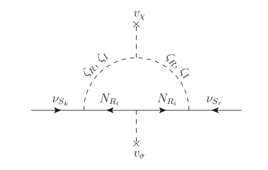
Figure 1: Feynman diagram for the generation of the Majorana neutrino mass $\mu$ via a loop involving the new particles from the dark sector, $N_{R}$ and $\zeta$. The indices run as follows: $i=1,2,3$ and $k,r=1,2$.

We show in Fig. 1 the relevant diagram generating the Majorana mass term for the $\nu_{S}$ sterile neutrinos, which involves a loop with the $N_{R}$ fields and the inert scalar $\zeta$. Notice that both real and imaginary components of the scalar singlet $\zeta$ participate in the diagram, coupled to the scalar singlet $\chi$ via the trilinear coupling $\eta_{\mu}$ defined in Eq. (1), which is at the same time responsible for generating the mass splitting between $\zeta_{R}$ and $\zeta_{I}$ in Eq. (13). From this diagram, we obtain the one-loop contribution given by

$$\mu_{\rm 1-loop}^{kr}=\frac{y_{\zeta}^{ki}y_{\zeta}^{ri}m_{N_{i}}}{16\pi^{2}}\,\left\{\frac{m_{\zeta_{R}}^{2}}{m_{\zeta_{R}}^{2}-m_{N_{i}}^{2}}\log\left(\frac{m_{\zeta_{R}}^{2}}{m_{N_{i}}^{2}}\right)-\frac{m_{\zeta_{I}}^{2}}{m_{\zeta_{I}}^{2}-m_{N_{i}}^{2}}\log\left(\frac{m_{\zeta_{I}}^{2}}{m_{N_{i}}^{2}}\right)\right\}\,,$$ (17)

where we have assumed, without lost of generality, that the submatrix $m_{N}$ is diagonal. This non-zero $\mu$ matrix triggers the ISS mechanism in the $(\nu_{L},\nu_{R}^{C},\nu_{S}^{C})$ sector, generating masses for the active neutrinos of the order $m_{\nu}\sim\mu\,m_{D}^{2}/M^{2}$ and mass splittings for the pairs of sterile neutrinos of $\mathcal{O}(\mu)$, thus implying that the sterile neutrinos form pseudo-Dirac pairs.

As usual, a successful ISS realization requires a light $\mu$ scale, in particular $\mu\ll m_{D},M$, which occurs naturally in our model. In order to explore this feature in detail, let us start assuming a small mass splitting between the real and imaginary components of $\zeta$, i.e.

$$m_{\zeta_{R}}^{2}-m_{\zeta_{I}}^{2}=2v_{\chi}\eta_{\mu}\ll 2m_{\zeta}^{2}\equiv m_{\zeta_{R}}^{2}+m_{\zeta_{I}}^{2}\ .$$ (18)

Then, we can write

$$\mu_{\rm 1-loop}^{kr}\simeq\frac{y_{\zeta}^{ki}y_{\zeta}^{ri}}{8\pi^{2}}\,v_{\chi}\eta_{\mu}\,m_{N_{i}}\,\frac{m_{\zeta}^{2}-m_{N_{i}}^{2}+m_{N_{i}}^{2}\log m_{N_{i}}^{2}/m_{\zeta}^{2}}{(m_{\zeta}^{2}-m_{N_{i}}^{2})^{2}}\,.$$ (19)

From this equation, we see that the generated $\mu$ scale is suppressed by a loop factor, and it is proportional to the $y_{\zeta}$ and $\eta_{\mu}$ parameters. Interestingly, in the limit when these parameters are zero, together with the quartic coupling $\lambda^{\prime}_{\zeta}$, the Lagrangian becomes invariant under a global $U(1)_{\zeta}$ symmetry under which only the $\zeta$ fields are charged. In this sense, it is technically natural to consider these three parameters, and in particular $y_{\zeta}$ and $\eta_{\mu}$, to be small, a fact that further suppresses the $\mu$ scale. Therefore, our model predicts a small scale for the ISS $\mu$ term, which is suppressed by a loop factor and three powers of technically natural small parameters.

Furthermore, Eq. (19) exhibits the link between the light neutrino masses and the dark sector, and can be used to relate the relevant scales for both sectors. In order to do that, let us recall again that in the ISS mechanism the light active neutrino mass scale $m_{\nu}$ is of the order of

$$m_{\nu}\approx\mu\,\frac{m_{D}^{2}}{M^{2}}\approx\mu\,\big{|}U_{\nu N}\big{|}^{2}\,,$$ (20)

with $U_{\nu N}$ the active sterile neutrino mixing. This mixing modifies the neutral and charged lepton currents, leading thus to numerous constraints. Cosmological observations [60, 61, 62, 63] put severe constraints on neutral leptons with a mass below $\sim 200$ MeV. Additional strong bounds for sterile neutrinos lighter that the mass of the W gauge boson are imposed from several laboratory searches, see for instance Refs. [64, 65, 66]. In the following, we focus on the case where the sterile neutrinos realizing the ISS mechanism are heavier than the electroweak scale, which are mainly constrained by electroweak observables and charged lepton flavor transitions [67]. A global fit analysis to these observables [68] imposes bounds on their mixings of the order $|U_{\nu N}|^{2}\lesssim 10^{-3}$, which implies that $\mu\gtrsim\mathcal{O}(1)$ keV in order to reproduce $\sim 1$ eV neutrino masses.

On the other hand, Eq. (19) can be studied in two interesting limits, both related to the mass hierarchy between the lightest $N_{R}$ and $\zeta$ defining the DM candidate in our model. In the case where $m_{N}\ll m_{\zeta}$, the model contains a fermionic DM candidate with mass $m_{N}$, and the $\mu$ scale of the ISS can be expressed, using Eq. (18), as

$$\mu\approx\frac{y_{\zeta}^{2}}{16\pi^{2}}\,\frac{\Delta m_{\zeta}^{2}}{m_{\zeta}^{2}}\,m_{N}\approx 6\,{\rm keV}\leavevmode\nobreak\ \bigg{(}\frac{y_{\zeta}}{10^{-2}}\bigg{)}^{2}\,\bigg{(}\frac{\Delta m_{\zeta}^{2}/m_{\zeta}^{2}}{10^{-2}}\bigg{)}\,\bigg{(}\frac{m_{N}}{1\,{\rm TeV}}\bigg{)}\,.$$ (21)

In the opposite limit of $m_{\zeta}\ll m_{N}$, we have a scalar DM with mass $m_{\zeta}$, and

$$\mu\approx\frac{y_{\zeta}^{2}}{16\pi^{2}}\,\frac{\Delta m_{\zeta}^{2}}{m_{\zeta}^{2}}\,\frac{m_{\zeta}^{2}}{m_{N}}\Big{(}\log\frac{m_{N}^{2}}{m_{\zeta}^{2}}-1\Big{)}\approx 1\,{\rm keV}\bigg{(}\frac{y_{\zeta}}{10^{-2}}\bigg{)}^{2}\,\bigg{(}\frac{\Delta m_{\zeta}^{2}/m_{\zeta}^{2}}{10^{-2}}\bigg{)}\,\bigg{(}\frac{m_{\zeta}}{1\,{\rm TeV}}\bigg{)}^{2}\bigg{(}\frac{10\,{\rm TeV}}{m_{N}}\bigg{)}\,,$$ (22)

where we have neglected the logarithmic dependence in the last step. Notice that the case $m_{N}\sim m_{\zeta}$ leads to the same $\mu$ term than in the case $m_{N}\ll m_{\zeta}$, with just an additional factor of $1/2$. From the above equations, we see that our model can easily generate the correct scale for the ISS $\mu$ term, with a DM candidate at the TeV scale, and relatively small $y_{\zeta}$ and $\Delta m_{\zeta}^{2}/m_{\zeta}^{2}$ (and thus $\eta_{\mu}$), which are protected by the accidental $U(1)_{\zeta}$ symmetry.

In conclusion, our model connects the ISS $\mu$ term with the dark sector via the loop diagram in Fig. 1, in a similar fashion as the scotogenic model [57] does for neutrino mass generation. Notice however that in the original scotogenic model the dark sector generates directly small radiative masses for the active neutrinos, while in our model the dark sector generates only the Majorana masses for the sterile neutrinos $\nu_{S}$, which then induce masses for active neutrinos via the ISS mechanism. In this sense, our model provides a scotogenic origin for the ISS $\mu$ term. A similar idea has been proposed, for instance, in Refs. [36, 39, 40, 46], with different particle content and symmetries than ours, and without linking it to the gauging of $U(1)_{B-L}$, as done in this work.

4 Dark matter

The residual $\mathbb{Z}_{2}$ symmetry protects the lightest odd state of the dark sector, rendering it a viable candidate for DM. Depending on the mass hierarchy, we could have scalar or fermionic DM candidates if $\zeta$ or $N_{R}$ are the lightest states, respectively. The phenomenology of the WIMP paradigm of these two cases will be studied in the following.

4.1 Scalar dark matter

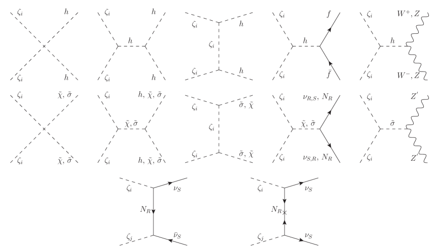
Figure 2: Main channels contributing to the production of scalar DM $\zeta_{i}$, with $i$ identifying the lightest state between the real and imaginary part of $\zeta$, and $j=R$, $I$. Crossed diagrams are not shown, although taken into account in the analysis. $f$ labels all the fermion fields coupled to the Higgs.

In this section, we consider the case where the DM candidate is the lightest component of $\zeta$, either its real or its imaginary part. In the early Universe, it can be produced out of the SM thermal bath by the WIMP mechanism, via the different 2-to-2 scatterings presented in Fig. 2. DM can annihilate into SM Higgs bosons via the contact interaction, the $s$-channel exchange of a Higgs, or the $t$- and $u$-channel mediation of a $\zeta$. It is also possible to have a scattering into SM charged fermions and vector bosons, mediated by the Higgs portal. Additionally, the new scalars $\tilde{\sigma}$ and $\tilde{\chi}$ could be in the final state or mediate the annihilation, as shown in the second row of Fig. 2. Finally, DM can annihilate into neutrinos via the $t$-channel exchange of $N_{R}$ (last row). This latter channel exists not only for the DM annihilation but also for the coannihilation $\zeta_{R}$-$\zeta_{I}$, which is typically relevant if the mass splitting, see Eq. (13), is smaller that $\sim 20\%$ [69]. However, it is interesting to note that both the annihilation and the coannihilation into active neutrinos depends on the active-sterile mixing angles (to the fourth power), which are suppressed at high temperature (i.e. at $T\gtrsim 200$ MeV) due to over dominating thermal masses of the active neutrinos [70, 71, 72], and therefore these channels are subdominant.

In the decoupling limit ($\lambda_{\phi\sigma}=\lambda_{\phi\chi}=0$), where $h$ behaves as the SM Higgs, and if $\zeta$ is lighter than the other dark sector particles, the main annihilation channels correspond to the ones on the first row of Fig. 2, and the present scenario reduces to the scalar singlet DM model [73, 74, 75]. Figure 3 shows with a black line the values for the Higgs portal coupling $\lambda_{\phi\zeta}$ as a function of the DM mass $m_{\zeta}$ required to reproduce the whole observed DM abundance. A full numerical computation has been performed using MicrOMEGAs [76, 77].

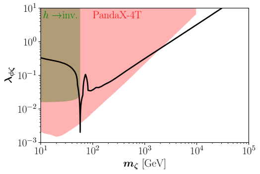
Figure 3: Scalar DM. Parameter space that reproduces the whole observed DM abundance (black thick line). The color-shaded areas are in tension with the invisible decay of the Higgs (brown) or PandaX-4T results (red).

This scenario is constrained by collider measurements [78, 79, 80, 81, 82, 83, 84]. In particular, strong bounds on the invisible decay of the Higgs apply for $m_{\zeta}\lesssim 60\ \text{GeV}$, as one can have $h\to\zeta_{R}\zeta_{R}$ and $h\to\zeta_{I}\zeta_{I}$. The corresponding decay width is given by

$$\Gamma_{h\to\zeta\zeta}=\frac{\lambda_{\phi\zeta}^{2}}{32\pi}\frac{v^{2}}{m_{h}}\left[\sqrt{1-4\frac{m_{\zeta_{R}}^{2}}{m_{h}^{2}}}+\sqrt{1-4\frac{m_{\zeta_{I}}^{2}}{m_{h}^{2}}}\right].$$ (23)

A recent combination of searches with the ATLAS experiment found an upper bound for this branching ratio $\text{Br}(h\to\text{inv})<0.11$ at 95% CL [85]. The corresponding excluded region is overlaid in brown in Fig. 3.

The DM direct detection can further constrain the parameter space. The corresponding spin-independent DM-nucleon scattering cross section is given by [86, 87, 88, 89, 90]

$$\sigma\simeq\frac{\lambda_{\phi\zeta}^{2}\,f_{n}}{4\pi}\frac{\mu_{\zeta}^{2}\,m_{n}^{2}}{m_{h}^{4}\,m_{\zeta}^{2}}\,,$$ (24)

where $m_{n}$ is the nucleon mass, $\mu_{\zeta}\equiv m_{\zeta}\,m_{n}/(m_{\zeta}+m_{n})$ is the DM-nucleon reduced mass, and $f_{n}\sim 0.3$ is the hadron matrix element. In Fig. 3 the recent limits from the PandaX-4T experiment [91] are shown in red.

Additionally, indirect detection with $\gamma$-rays and antimatter could further constrain this scenario [92, 93, 94, 95, 96, 97, 98, 99], however the limits are comparable to the ones coming from direct detection and thus we do not show them in Fig. 3. The combination of the direct detection bound together with the invisible decay width excludes a large fraction of the parameter space, letting unconstrained the narrow mass window close to the Higgs funnel ($m_{\zeta}\sim m_{h}/2$), and the region above the TeV, i.e., 2 TeV $\lesssim m_{\zeta}\lesssim 30$ TeV. Notice that larger masses would require non-perturbative $\lambda_{\phi\zeta}$ in order to not overclose the Universe.

Before closing this section, it is interesting to note that in the present scenario alternatives to the WIMP mechanism exists. For example, DM could also have been produced non-thermally in the early Universe via the FIMP mechanism [100, 101, 102, 103, 104]. In that case, much smaller Higgs portal couplings are required $\mathcal{O}(\lambda_{\phi\zeta})\sim 10^{-11}$ with a broader mass range [105, 106, 107]. Additionally, if the Higgs portal coupling is suppressed and DM has sizable self-interactions due to a quartic coupling of order $\mathcal{O}(\lambda_{\zeta})\sim 1$, thermalization in the dark sector could have a strong impact on the DM abundance [108, 109, 110]. Moreover, DM could have been Hawking radiated by primordial black holes [111]. Finally, this model has also been studied in the framework of non-standard cosmologies [112, 113, 114, 115].

4.2 Fermionic dark matter

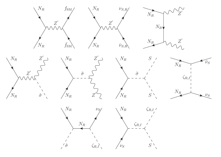
Figure 4: Main channels contributing to the production of fermionic DM. $f_{\text{SM}}$ indicates all the SM fermions coupled to the $Z^{\prime}$ and $S=h$, $\tilde{\sigma}$, $\tilde{\chi}$, and $\zeta_{R,I}$.

In this case, the DM candidate is the lightest $N_{R_{i}}$ state. In the early Universe, DM can annihilate into $a)$ SM fermions and sterile neutrinos $\nu_{R}$ and $\nu_{S}$ mediated via the $s$-channel exchange of a $Z^{\prime}$, together with the annihilation into a pair of $Z^{\prime}$ (first row in Fig. 4), or $b)$ $Z^{\prime}\,\sigma$, $Z^{\prime}\,Z^{\prime}$, a couple of scalars or neutral fermions (second row). Finally, $c)$ DM can coannihilate with $\tilde{\sigma}$ or an active neutrino via the active-sterile mixing (last row). As in the case of scalar DM, here some processes are typically subdominant because the coupling $\lambda_{\phi\sigma}$ has to be very small to avoid tension with Higgs physics, and because the active-sterile mixing angles are suppressed at high temperatures.

If the DM $N_{R}$ is the lightest state of the dark sector, most of the channels described in Fig. 4 are kinematically closed, and therefore the annihilation into SM states via the exchange of a $Z^{\prime}$ boson tends to be dominant. In that case the DM phenomenology is determined by three parameters: $m_{N}$, $M_{Z^{\prime}}$ and the gauge coupling $g_{B-L}$. Figure 5 shows contours for the values of the coupling $g_{B-L}$ required in order to successfully reproduce the whole observed DM abundance in the plane $[m_{N},\,M_{Z^{\prime}}]$ (blue thick lines). The red dotted line corresponds to the resonant annihilation case ($M_{Z^{\prime}}=2\,m_{N}$), and separates the regimes $M_{Z^{\prime}}\gg 2\,m_{N}$, where DM annihilates into SM pairs via the $s$-channel exchange of a $Z^{\prime}$, from the regime $M_{Z^{\prime}}\ll 2\,m_{N}$, where DM annihilates into a couple of $Z^{\prime}$ dominantly via the $t$-channel mediation of $N_{R}$. Notice that in the latter limit, also the first 3 diagrams of the second row are relevant, since we could expect $m_{\tilde{\sigma}^{\prime}}$ to be of the same order of $M_{Z}^{\prime}$. Nevertheless, achieving the hierarchy $M_{Z^{\prime}}\ll m_{N}$ for $g_{B-L}\gtrsim 1$ requires large couplings $y_{\sigma}$, leading to the non-perturbative regime shown in gray in Fig. 5, and thus this hierarchy is disfavored. Again, we have performed a full numerical computation with MicrOMEGAs.

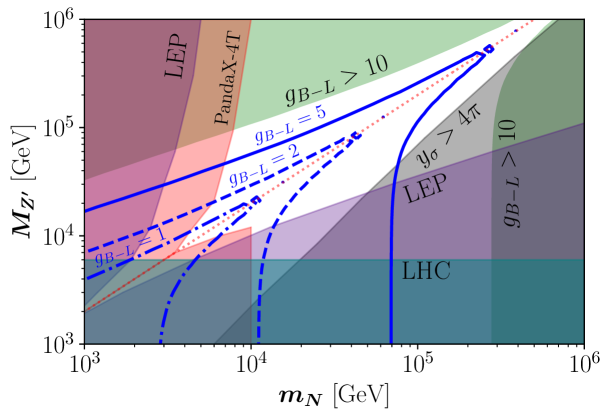
Figure 5: Fermionic DM. Contours for the coupling $g_{B-L}$ required in order to reproduce the whole observed DM abundance (thick blue lines). The color-shaded areas are in tension with LHC searches for $Z^{\prime}$ gauge bosons (blue), LEP measurements of $e^{+}e^{-}\to\ell^{+}\ell^{-}$ (purple), direct DM searches from PandaX-4T (red), and the perturbative bounds on $g_{B-L}$ (green) and $y_{\sigma}$ (gray). The red dotted line corresponds to $2\,m_{N}=M_{Z^{\prime}}$.

In the limit of small momentum transfer, the $Z^{\prime}$ exchange leads to a spin-independent scattering with nucleons. The corresponding cross section per nucleon is given by [116]

$$\sigma\simeq\frac{g_{B-L}^{4}}{\pi}\frac{m_{n}^{2}\,m_{N}^{2}}{(m_{n}+m_{N})^{2}\,M_{Z^{\prime}}^{4}}\,,$$ (25)

however, in our numerical analysis we used MicrOMEGAs to determine the values of the spin-independent scattering cross section per nucleon. PandaX-4T results provide strong bounds to this scenario with large $g_{B-L}$ couplings, constraining spin-independent cross section up to DM masses of 10 TeV. Lighter DM masses ($m_{N}\gtrsim 3$ TeV) are only allowed near the resonance $m_{N}\simeq 2\,M_{Z^{\prime}}$.

On the other hand, there are several bounds on the massive gauge boson of $U(1)_{B-L}$ [117]. For $M_{Z^{\prime}}$ of few TeV and the large $g_{B-L}$ couplings needed in Fig. 5, the $Z^{\prime}$ would be copiously produced at the LHC, decaying to electrons and muons 20-30% of the times, depending if the $Z^{\prime}$ to the sterile neutrinos channels are kinematically open or not. Consequently, LHC searches [55, 56] exclude all the viable parameter space for $Z^{\prime}$ lighter than 6 TeV. Furthermore, LEP measurements of $e^{+}e^{-}\to\ell^{+}\ell^{-}$ [118] were sensitive to heavy $Z^{\prime}$ bosons, constraining the mass to be $M_{Z^{\prime}}>6\,g_{B-L}$ TeV [119]. Finally, we note that the required gauge coupling $g_{B-L}$ should be higher than $\sim 0.7$ in order to successfully reproduce the whole observed DM abundance. Nevertheless, too large $g_{B-L}$ couplings would violate perturbativity, leading to a well-defined allowed area in the parameter space that will be further probed in future experiments.

5 Conclusions

We have constructed a low-scale seesaw model with a local $U(1)_{B-L}$ symmetry, where some of the sterile neutrinos acquire a small Majorana mass radiatively, triggering then an inverse seesaw mechanism to generate tiny masses for the active neutrinos.

In our proposed model, the SM gauge symmetry is supplemented by the spontaneously broken local $U(1)_{B-L}$ and discrete $\mathbb{Z}_{4}$ symmetries, an extended scalar sector and additional fermionic singlets. The latter allows us to cancel the gauge anomalies of $B-L$ and to realize an ISS mechanism for neutrino mass generation. The discrete $\mathbb{Z}_{4}$, spontaneously broken to a residual $\mathbb{Z}_{2}$, forbids the sterile neutrinos to acquire tree-level Majorana masses, which is instead generated from a one-loop diagram involving the dark sector particles. This loop suppression, together with the smallness of the couplings involved in the loop, provides a natural explanation for the smallness of the ISS $\mu$ term.

Additionally, our model contains both scalar and fermionic DM candidates, whose stability is ensured from the residual $\mathbb{Z}_{2}$ symmetry. We have shown that this model, in addition to providing an origin of the ISS mechanism, reproduces successfully the measured value of the DM abundance and is consistent with the constraints arising from the DM direct detection, invisible Higgs decays and LHC $Z^{\prime}$ searches. The consistency with all these constraints restricts the mass of the scalar DM candidate to be either $m_{h}/2$ or larger than about 2 TeV for values of the Higgs portal coupling of order unity. On the other hand, in the scenario of fermionic DM candidate, the aforementioned constraints set the masses of the fermionic DM component and the $Z^{\prime}$ gauge boson to heavier than few TeV, and the $U(1)_{B-L}$ gauge coupling such that $g_{B-L}\gtrsim 0.7$. Smaller couplings induce a DM overproduction that overclose the Universe. Alternatively, much higher couplings generate a DM underabundance, compatible with a multicomponent DM scenario. Future DM searches covering heavy DM candidates, further input from LHC and new detailed measurements of $e^{+}e^{-}\to\ell^{+}\ell^{-}$ at future lepton colliders will ultimately add new constraints on the $Z^{\prime}$ mass and $g_{B-L}$, as well as on the sterile fermion masses, rendering our scenario testable.

Appendix A Anomaly cancellation

Through the following conditions, we have checked the gauge and gravitational anomaly cancellation

$$A_{\left[SU\left(3\right)_{C}\right]^{2}U\left(1\right)_{B-L}} =2\sum_{i=1}^{3}\left(B-L\right)_{q_{iL}}-\sum_{i=1}^{3}\left[\left(B-L\right)_{u_{iR}}+\left(B-L\right)_{d_{iR}}\right],$$ (26)

$$A_{\left[SU\left(2\right)_{L}\right]^{2}U\left(1\right)_{X}} =2\sum_{i=1}^{3}\left(B-L\right)_{\ell_{iL}}+6\sum_{i=1}^{3}\left(B-L\right)_{q_{iL}},$$ (27)

$$A_{\left[U\left(1\right)_{Y}\right]^{2}U\left(1\right)_{B-L}} =2\sum_{i=1}^{3}\left[Y_{\ell_{iL}}^{2}\left(B-L\right)_{\ell_{iL}}+3Y_{q_{iL}}^{2}\left(B-L\right)_{q_{iL}}\right]$$

$$-\sum_{i=1}^{3}\left[Y_{\ell_{iR}}^{2}\left(B-L\right)_{\ell_{iR}}+3Y_{u_{iR}}^{2}\left(B-L\right)_{u_{iR}}+3Y_{d_{iR}}^{2}\left(B-L\right)_{d_{iR}}\right],$$ (28)

$$A_{\left[U\left(1\right)_{B-L}\right]^{2}U\left(1\right)_{Y}} =2\sum_{i=1}^{3}\left[Y_{\ell_{iL}}\left(B-L\right)_{\ell_{iL}}^{2}+3Y_{q_{iL}}\left(B-L\right)_{q_{iL}}^{2}\right]$$

$$-\sum_{i=1}^{3}\left[Y_{\ell_{iR}}\left(B-L\right)_{\ell_{iR}}^{2}+3Y_{u_{iR}}\left(B-L\right)_{u_{iR}}^{2}+3Y_{d_{iR}}\left(B-L\right)_{d_{iR}}^{2}\right],$$ (29)

$$A_{\left[U\left(1\right)_{B-L}\right]^{3}} =\sum_{i=1}^{3}\left[2\left(B-L\right)_{\ell_{iL}}^{3}+6\left(B-L\right)_{q_{iL}}^{3}-3\left(B-L\right)_{u_{iR}}^{3}-3\left(B-L\right)_{d_{iR}}^{3}\right]$$

$$-\sum_{i=1}^{3}\left[\left(B-L\right)_{\ell_{iR}}^{3}+\left(B-L\right)_{N_{R_{i}}}^{3}\right]+\sum_{k=1}^{2}\left[\left(B-L\right)_{\nu_{R_{k}}}^{3}+\left(B-L\right)_{\nu_{S_{k}}}^{3}\right],$$ (30)

$$A_{\left[\text{Gravity}\right]^{2}U\left(1\right)_{B-L}} =\,\sum_{i=1}^{3}\left[2\left(B-L\right)_{\ell_{iL}}+6\left(B-L\right)_{q_{iL}}-3\left(B-L\right)_{u_{iR}}-3\left(B-L\right)_{d_{iR}}\right]$$

$$-\sum_{i=1}^{3}\left[\left(B-L\right)_{\ell_{iR}}+\left(B-L\right)_{N_{R_{i}}}\right]+\sum_{k=1}^{2}\left[\left(B-L\right)_{\nu_{R_{k}}}+\left(B-L\right)_{\nu_{S_{k}}}\right],$$ (31)

with $A$ the anomaly coefficients appearing in the triangular amplitude involving gauge bosons (corresponding to the groups indicated in the subindices) in the external lines and SM fermions in the internal lines. Here $B-L$ and $Y$ refer respectively to the charges under $U(1)_{B-L}$ and $U(1)_{Y}$, as given in Table 1.

Appendix B Stability and unitarity conditions

In order to determine the stability conditions of the scalar potential, one has to analyze its quartic terms because they will dominate the behavior of the scalar potential in the region of very large values of the field components. To this end, we introduce the following hermitian bilinear combination of the scalar fields

$$a=\phi^{\dagger}\phi,\hskip 28.45274ptb=\sigma^{\ast}\sigma,\hskip 28.45274ptc=\zeta^{\ast}\zeta,\hskip 28.45274ptd=\chi^{2},\hskip 28.45274pte=\zeta^{2},$$ (32)

and rewrite the quartic terms of the scalar potential as follows:

$$V_{4} = \left(\sqrt{\lambda}a-\sqrt{\lambda_{\sigma}}b\right)^{2}+\left(\sqrt{\lambda}a-\sqrt{\lambda_{\zeta}}c\right)^{2}+\left(\sqrt{\lambda}a-\frac{1}{2}\sqrt{\lambda_{\chi}}d\right)^{2}+\left(\sqrt{\lambda_{\sigma}}b-\sqrt{\lambda_{\zeta}}c\right)^{2}$$

$$+\left(\sqrt{\lambda_{\sigma}}b-\frac{1}{2}\sqrt{\lambda_{\chi}}d\right)^{2}+\left(\sqrt{\lambda_{\zeta}}c-\frac{1}{2}\sqrt{\lambda_{\chi}}d\right)^{2}-2\left(\lambda a^{2}+\lambda_{\sigma}b^{2}+\lambda_{\zeta}c^{2}\right)$$

$$+\left(\lambda_{\phi\sigma}+2\sqrt{\lambda\lambda_{\sigma}}\right)ab+\left(\lambda_{\phi\zeta}+2\sqrt{\lambda\lambda_{\zeta}}\right)ac+\left(\lambda_{\phi\chi}+\sqrt{\lambda\lambda_{\chi}}\right)ad$$

$$+\left(\lambda_{\zeta\sigma}+2\sqrt{\lambda_{\sigma}\lambda_{\zeta}}\right)bc+\left(\lambda_{\zeta\chi}+\sqrt{\lambda_{\zeta}\lambda_{\chi}}\right)cd+\left(\lambda_{\sigma\chi}+\sqrt{\lambda_{\sigma}\lambda_{\chi}}\right)bd+\lambda^{\prime}_{\zeta}\left(e^{2}+h.c\right)\,.$$

Following the procedure used for analyzing the stability described in Refs. [120, 121], we find that our scalar potential will be stable when the following conditions are fulfilled:

$$\lambda\geq 0,\hskip 28.45274pt \lambda_{\sigma} \geq 0,\hskip 28.45274pt\lambda_{\zeta}\geq 0,\hskip 28.45274pt\lambda_{\chi}\geq 0,\hskip 28.45274pt\lambda^{\prime}_{\zeta}\geq 0,$$

$$\lambda_{\phi\sigma}+2\sqrt{\lambda\lambda_{\sigma}} \geq 0,\hskip 28.45274pt\lambda_{\phi\zeta}+2\sqrt{\lambda\lambda_{\zeta}}\geq 0,\hskip 28.45274pt\lambda_{\phi\chi}+\sqrt{\lambda\lambda_{\chi}}\geq 0,$$

$$\lambda_{\zeta\sigma}+2\sqrt{\lambda_{\sigma}\lambda_{\zeta}} \geq 0,\hskip 28.45274pt\lambda_{\zeta\chi}+\sqrt{\lambda_{\zeta}\lambda_{\chi}}\geq 0,\hskip 28.45274pt\lambda_{\sigma\chi}+\sqrt{\lambda_{\sigma}\lambda_{\chi}}\geq 0.$$ (34)

Regarding unitarity conditions, they are imposed to avoid that the scattering amplitudes involving physical scalars and longitudinal gauge bosons grow too much with energy. In practice, we consider the partial wave expansion, given for an amplitude $\mathcal{M}$ by

$$\mathcal{M}(\theta)=16\pi\,\sum_{\ell=0}^{\infty}(2\ell+1)\,a_{\ell}\,P_{\ell}(\cos\theta)\,,$$ (35)

with $P_{\ell}$ the Legendre polynomials and $a_{\ell}$ the partial wave of order $\ell$, and require that the partial waves are bounded from above for any of the possible $2\to 2$ scatterings.

This process can be simplified thanks to the equivalence theorem [122, 123, 124, 125], as explained for instance, in Ref. [121]. The main idea is that the high-energy behavior of these scatterings can be described using the unphysical scalar particles. Moreover, these scatterings will be dominated by the dimensionless quartic couplings in Eq. (1), which contribute only to the $\ell=0$ partial wave, bounded to be $|a_{0}|<1$. Then, we can easily compute the high-energy scattering amplitudes in the unphysical basis, where all the interactions are just given by the quartic couplings, and then obtain the physical unitarity conditions by requiring that the eigenvalues of this $\mathcal{S}$-matrix are lower than $16\pi$.

In our scalar sector, we can have two kinds of $2\to 2$ scatterings, as the electric charge needs to be conserved. From one side, we can have electrically neutral pairs defining the basis

$$\left(\phi^{-}\phi^{+},\,\frac{hh}{\sqrt{2}},\,\frac{\phi_{Z}\phi_{Z}}{\sqrt{2}},\,\frac{\tilde{\sigma}\tilde{\sigma}}{\sqrt{2}},\,\frac{\sigma_{Z^{\prime}}\sigma_{Z^{\prime}}}{\sqrt{2}},\,\frac{\tilde{\chi}\tilde{\chi}}{\sqrt{2}},\,\frac{\zeta_{R}\zeta_{R}}{\sqrt{2}},\,\frac{\zeta_{I}\zeta_{I}}{\sqrt{2}},\,\zeta_{R}\zeta_{I}\right)\,,$$ (36)

with the factor $1/\sqrt{2}$ for identical particles, which leads to the following scattering matrix,

$$\mathcal{S}_{N}={\footnotesize\left(\begin{array}[]{ccccccccc}4\lambda&\sqrt{2}\lambda&\sqrt{2}\lambda&\lambda_{\phi\sigma}\nicefrac{{}}{{\sqrt{2}}}&\lambda_{\phi\sigma}\nicefrac{{}}{{\sqrt{2}}}&\sqrt{2}\lambda_{\phi\chi}&\lambda_{\phi\zeta}\nicefrac{{}}{{\sqrt{2}}}&\lambda_{\phi\zeta}\nicefrac{{}}{{\sqrt{2}}}&0\\ \sqrt{2}\lambda&3\lambda&\lambda&\lambda_{\phi\sigma}\nicefrac{{}}{{2}}&\lambda_{\phi\sigma}\nicefrac{{}}{{2}}&\lambda_{\phi\chi}&\lambda_{\phi\zeta}\nicefrac{{}}{{2}}&\lambda_{\phi\zeta}\nicefrac{{}}{{2}}&0\\ \sqrt{2}\lambda&\lambda&3\lambda&\lambda_{\phi\sigma}\nicefrac{{}}{{2}}&\lambda_{\phi\sigma}\nicefrac{{}}{{2}}&\lambda_{\phi\chi}&\lambda_{\phi\zeta}\nicefrac{{}}{{2}}&\lambda_{\phi\zeta}\nicefrac{{}}{{2}}&0\\ \lambda_{\phi\sigma}\nicefrac{{}}{{\sqrt{2}}}&\lambda_{\phi\sigma}\nicefrac{{}}{{2}}&\lambda_{\phi\sigma}\nicefrac{{}}{{2}}&3\lambda_{\sigma}&\lambda_{\sigma}&\lambda_{\sigma\chi}&\lambda_{\zeta\sigma}\nicefrac{{}}{{2}}&\lambda_{\zeta\sigma}\nicefrac{{}}{{2}}&0\\ \lambda_{\phi\sigma}\nicefrac{{}}{{\sqrt{2}}}&\lambda_{\phi\sigma}\nicefrac{{}}{{2}}&\lambda_{\phi\sigma}\nicefrac{{}}{{2}}&\lambda_{\sigma}&3\lambda_{\sigma}&\lambda_{\sigma\chi}&\lambda_{\zeta\sigma}\nicefrac{{}}{{2}}&\lambda_{\zeta\sigma}\nicefrac{{}}{{2}}&0\\ \sqrt{2}\lambda_{\phi\chi}&\lambda_{\phi\chi}&\lambda_{\phi\chi}&\lambda_{\sigma\chi}&\lambda_{\sigma\chi}&3\lambda_{\chi}&\lambda_{\zeta\chi}&\lambda_{\zeta\chi}&0\\ \lambda_{\phi\zeta}\nicefrac{{}}{{\sqrt{2}}}&\lambda_{\phi\zeta}\nicefrac{{}}{{2}}&\lambda_{\phi\zeta}\nicefrac{{}}{{2}}&\lambda_{\zeta\sigma}\nicefrac{{}}{{2}}&\lambda_{\zeta\sigma}\nicefrac{{}}{{2}}&\lambda_{\zeta\chi}&3\lambda_{\zeta}+6\lambda^{\prime}_{\zeta}&\lambda_{\zeta}-6\lambda^{\prime}_{\zeta}&0\\ \lambda_{\phi\zeta}\nicefrac{{}}{{\sqrt{2}}}&\lambda_{\phi\zeta}\nicefrac{{}}{{2}}&\lambda_{\phi\zeta}\nicefrac{{}}{{2}}&\lambda_{\zeta\sigma}\nicefrac{{}}{{2}}&\lambda_{\zeta\sigma}\nicefrac{{}}{{2}}&\lambda_{\zeta\chi}&\lambda_{\zeta}-6\lambda^{\prime}_{\zeta}&3\lambda_{\zeta}+6\lambda^{\prime}_{\zeta}&0\\ 0&0&0&0&0&0&0&0&2\lambda_{\zeta}-12\lambda^{\prime}_{\zeta}\end{array}\right)}.$$ (37)

From the other side, considering electrically charged pairs and taking the basis $(h\phi^{+},\phi_{Z}\phi^{+},\tilde{\sigma}\phi^{+},\\ \sigma_{Z^{\prime}}\phi^{+},\tilde{\chi}\phi^{+},\zeta_{R}\phi^{+},\zeta_{I}\phi^{+})$, we have

$$\mathcal{S}_{C}={\rm diag}\left(2\lambda,\,2\lambda,\,\lambda_{\phi\sigma},\,\lambda_{\phi\sigma},\,2\lambda_{\phi\chi},\,\lambda_{\phi\zeta},\,\lambda_{\phi\zeta}\right).$$ (38)

The unitarity conditions imply that the modulus of the eigenvalues of $\mathcal{S}_{N}$ and $\mathcal{S}_{C}$ lie below $16\pi$.

References

- [1] Y. Cai, J. Herrero-García, M. A. Schmidt, A. Vicente, and R. R. Volkas, “From the trees to the forest: a review of radiative neutrino mass models,” Front. in Phys. 5 (2017) 63, arXiv:1706.08524 [hep-ph].
- [2] P. Minkowski, “ at a Rate of One Out of Muon Decays?,” Phys. Lett. B 67 (1977) 421–428.
- [3] T. Yanagida, “Horizontal gauge symmetry and masses of neutrinos,” Conf. Proc. C 7902131 (1979) 95–99.
- [4] S. L. Glashow, “The Future of Elementary Particle Physics,” NATO Sci. Ser. B 61 (1980) 687.
- [5] R. N. Mohapatra and G. Senjanovic, “Neutrino Mass and Spontaneous Parity Nonconservation,” Phys. Rev. Lett. 44 (1980) 912.
- [6] M. Gell-Mann, P. Ramond, and R. Slansky, “Complex Spinors and Unified Theories,” Conf. Proc. C 790927 (1979) 315–321, arXiv:1306.4669 [hep-th].
- [7] J. Schechter and J. W. F. Valle, “Neutrino Masses in Theories,” Phys. Rev. D 22 (1980) 2227.
- [8] J. Schechter and J. W. F. Valle, “Neutrino Decay and Spontaneous Violation of Lepton Number,” Phys. Rev. D 25 (1982) 774.
- [9] I. Esteban, M. C. Gonzalez-Garcia, M. Maltoni, T. Schwetz, and A. Zhou, “The fate of hints: updated global analysis of three-flavor neutrino oscillations,” JHEP 09 (2020) 178, arXiv:2007.14792 [hep-ph].
- [10] P. F. de Salas, D. V. Forero, S. Gariazzo, P. Martínez-Miravé, O. Mena, C. A. Ternes, M. Tórtola, and J. W. F. Valle, “2020 global reassessment of the neutrino oscillation picture,” JHEP 02 (2021) 071, arXiv:2006.11237 [hep-ph].
- [11] A. Davidson and K. C. Wali, “Universal Seesaw Mechanism?,” Phys. Rev. Lett. 59 (1987) 393.
- [12] S. Iso, N. Okada, and Y. Orikasa, “Classically conformal extended Standard Model,” Phys. Lett. B 676 (2009) 81–87, arXiv:0902.4050 [hep-ph].
- [13] S. Iso, N. Okada, and Y. Orikasa, “The minimal model naturally realized at TeV scale,” Phys. Rev. D 80 (2009) 115007, arXiv:0909.0128 [hep-ph].
- [14] A. Datta, A. Elsayed, S. Khalil, and A. Moursy, “Higgs vacuum stability in the extended standard model,” Phys. Rev. D 88 no. 5, (2013) 053011, arXiv:1308.0816 [hep-ph].
- [15] A. Das, N. Okada, and N. Papapietro, “Electroweak vacuum stability in classically conformal B-L extension of the Standard Model,” Eur. Phys. J. C 77 no. 2, (2017) 122, arXiv:1509.01466 [hep-ph].
- [16] A. Das, S. Oda, N. Okada, and D.-s. Takahashi, “Classically conformal U(1)’ extended standard model, electroweak vacuum stability, and LHC Run-2 bounds,” Phys. Rev. D 93 no. 11, (2016) 115038, arXiv:1605.01157 [hep-ph].
- [17] T. Nomura and H. Okada, “Radiative neutrino mass in an alternative gauge symmetry,” Nucl. Phys. B 941 (2019) 586–599, arXiv:1705.08309 [hep-ph].
- [18] G. Chauhan, P. S. B. Dev, R. N. Mohapatra, and Y. Zhang, “Perturbativity constraints on and left-right models and implications for heavy gauge boson searches,” JHEP 01 (2019) 208, arXiv:1811.08789 [hep-ph].
- [19] A. Das, S. Goswami, K. N. Vishnudath, and T. Nomura, “Constraining a general inverse seesaw model from vacuum stability, dark matter and collider,” Phys. Rev. D 101 no. 5, (2020) 055026, arXiv:1905.00201 [hep-ph].
- [20] W. Abdallah, A. Awad, S. Khalil, and H. Okada, “Muon Anomalous Magnetic Moment and mu - e gamma in B-L Model with Inverse Seesaw,” Eur. Phys. J. C 72 (2012) 2108, arXiv:1105.1047 [hep-ph].
- [21] M. Aker et al., “First direct neutrino-mass measurement with sub-eV sensitivity,” arXiv:2105.08533 [hep-ex].
- [22] D. Wyler and L. Wolfenstein, “Massless Neutrinos in Left-Right Symmetric Models,” Nucl. Phys. B 218 (1983) 205–214.
- [23] R. N. Mohapatra and J. W. F. Valle, “Neutrino Mass and Baryon Number Nonconservation in Superstring Models,” Phys. Rev. D 34 (1986) 1642.
- [24] M. C. Gonzalez-Garcia and J. W. F. Valle, “Fast Decaying Neutrinos and Observable Flavor Violation in a New Class of Majoron Models,” Phys. Lett. B 216 (1989) 360–366.
- [25] S. M. Barr, “A Different seesaw formula for neutrino masses,” Phys. Rev. Lett. 92 (2004) 101601, arXiv:hep-ph/0309152.
- [26] M. Malinsky, J. C. Romao, and J. W. F. Valle, “Novel supersymmetric seesaw mechanism,” Phys. Rev. Lett. 95 (2005) 161801, arXiv:hep-ph/0506296.
- [27] H. Okada and T. Toma, “Fermionic Dark Matter in Radiative Inverse Seesaw Model with ,” Phys. Rev. D 86 (2012) 033011, arXiv:1207.0864 [hep-ph].
- [28] L. Basso, O. Fischer, and J. J. van der Bij, “Natural Z’ model with an inverse seesaw mechanism and leptonic dark matter,” Phys. Rev. D 87 no. 3, (2013) 035015, arXiv:1207.3250 [hep-ph].
- [29] Y. Kajiyama, H. Okada, and T. Toma, “Light Dark Matter Candidate in Gauged Radiative Inverse Seesaw,” Eur. Phys. J. C 73 no. 3, (2013) 2381, arXiv:1210.2305 [hep-ph].
- [30] E. Ma and R. Srivastava, “Dirac or inverse seesaw neutrino masses with gauge symmetry and flavor symmetry,” Phys. Lett. B 741 (2015) 217–222, arXiv:1411.5042 [hep-ph].
- [31] V. De Romeri, E. Fernandez-Martinez, J. Gehrlein, P. A. N. Machado, and V. Niro, “Dark Matter and the elusive in a dynamical Inverse Seesaw scenario,” JHEP 10 (2017) 169, arXiv:1707.08606 [hep-ph].
- [32] C.-Q. Geng and H. Okada, “Neutrino masses, dark matter and leptogenesis with gauge symmetry,” Phys. Dark Univ. 20 (2018) 13–19, arXiv:1710.09536 [hep-ph].
- [33] T. Nomura and H. Okada, “A radiative seesaw model with higher order terms under an alternative ,” Phys. Lett. B 781 (2018) 561–567, arXiv:1711.05115 [hep-ph].
- [34] T. Mondal and H. Okada, “Inverse seesaw and anomalies in extended two Higgs doublet model,” arXiv:2103.13149 [hep-ph].
- [35] E. Fernandez-Martinez, M. Pierre, E. Pinsard, and S. Rosauro-Alcaraz, “Inverse Seesaw, dark matter and the Hubble tension,” arXiv:2106.05298 [hep-ph].
- [36] E. Ma, “Radiative inverse seesaw mechanism for nonzero neutrino mass,” Phys. Rev. D 80 (2009) 013013, arXiv:0904.4450 [hep-ph].
- [37] F. Bazzocchi, “Minimal Dynamical Inverse See Saw,” Phys. Rev. D 83 (2011) 093009, arXiv:1011.6299 [hep-ph].
- [38] S. S. C. Law and K. L. McDonald, “Inverse seesaw and dark matter in models with exotic lepton triplets,” Phys. Lett. B 713 (2012) 490–494, arXiv:1204.2529 [hep-ph].
- [39] S. Fraser, E. Ma, and O. Popov, “Scotogenic Inverse Seesaw Model of Neutrino Mass,” Phys. Lett. B 737 (2014) 280–282, arXiv:1408.4785 [hep-ph].
- [40] A. Ahriche, S. M. Boucenna, and S. Nasri, “Dark Radiative Inverse Seesaw Mechanism,” Phys. Rev. D 93 no. 7, (2016) 075036, arXiv:1601.04336 [hep-ph].
- [41] A. E. Cárcamo Hernández, R. Martinez, and F. Ochoa, “Fermion masses and mixings in the 3-3-1 model with right-handed neutrinos based on the flavor symmetry,” Eur. Phys. J. C 76 no. 11, (2016) 634, arXiv:1309.6567 [hep-ph].
- [42] A. E. Cárcamo Hernández, S. Kovalenko, J. W. F. Valle, and C. A. Vaquera-Araujo, “Predictive Pati-Salam theory of fermion masses and mixing,” JHEP 07 (2017) 118, arXiv:1705.06320 [hep-ph].
- [43] A. E. Cárcamo Hernández, S. Kovalenko, J. W. F. Valle, and C. A. Vaquera-Araujo, “Neutrino predictions from a left-right symmetric flavored extension of the standard model,” JHEP 02 (2019) 065, arXiv:1811.03018 [hep-ph].
- [44] A. E. Cárcamo Hernández, H. N. Long, and V. V. Vien, “The first flavor 3-3-1 model with low scale seesaw mechanism,” Eur. Phys. J. C 78 no. 10, (2018) 804, arXiv:1803.01636 [hep-ph].
- [45] E. Bertuzzo, S. Jana, P. A. N. Machado, and R. Zukanovich Funchal, “Neutrino Masses and Mixings Dynamically Generated by a Light Dark Sector,” Phys. Lett. B 791 (2019) 210–214, arXiv:1808.02500 [hep-ph].
- [46] N. Rojas, R. Srivastava, and J. W. F. Valle, “Scotogenic origin of the Inverse Seesaw Mechanism,” arXiv:1907.07728 [hep-ph].
- [47] A. E. Cárcamo Hernández and S. F. King, “Littlest Inverse Seesaw Model,” Nucl. Phys. B 953 (2020) 114950, arXiv:1903.02565 [hep-ph].
- [48] A. E. Cárcamo Hernández, J. Marchant González, and U. J. Saldaña Salazar, “Viable low-scale model with universal and inverse seesaw mechanisms,” Phys. Rev. D 100 no. 3, (2019) 035024, arXiv:1904.09993 [hep-ph].
- [49] A. E. Cárcamo Hernández, Y. Hidalgo Velásquez, and N. A. Pérez-Julve, “A 3-3-1 model with low scale seesaw mechanisms,” Eur. Phys. J. C 79 no. 10, (2019) 828, arXiv:1905.02323 [hep-ph].
- [50] A. E. Cárcamo Hernández, D. T. Huong, and H. N. Long, “Minimal model for the fermion flavor structure, mass hierarchy, dark matter, leptogenesis, and the electron and muon anomalous magnetic moments,” Phys. Rev. D 102 no. 5, (2020) 055002, arXiv:1910.12877 [hep-ph].
- [51] A. E. C. Hernández and I. Schmidt, “A renormalizable left-right symmetric model with low scale seesaw mechanisms,” arXiv:2101.02718 [hep-ph].
- [52] A. E. Cárcamo Hernández, C. Espinoza, J. Carlos Gómez-Izquierdo, and M. Mondragón, “Fermion masses and mixings, dark matter, leptogenesis and muon anomaly in an extended 2HDM with inverse seesaw,” arXiv:2104.02730 [hep-ph].
- [53] T. Nomura, H. Okada, and P. Sanyal, “A radiatively induced inverse seesaw model with hidden gauge symmetry,” arXiv:2103.09494 [hep-ph].
- [54] A. E. C. Hernández, H. N. Long, M. L. Mora-Urrutia, N. H. Thao, and V. V. Vien, “Fermion masses and mixings and muon anomaly in a 3-3-1 model with family symmetry,” arXiv:2104.04559 [hep-ph].
- [55] ATLAS Collaboration, G. Aad et al., “Search for high-mass dilepton resonances using 139 fb-1 of collision data collected at 13 TeV with the ATLAS detector,” Phys. Lett. B 796 (2019) 68–87, arXiv:1903.06248 [hep-ex].
- [56] CMS Collaboration, A. M. Sirunyan et al., “Search for resonant and nonresonant new phenomena in high-mass dilepton final states at 13 TeV,” arXiv:2103.02708 [hep-ex].
- [57] E. Ma, “Verifiable radiative seesaw mechanism of neutrino mass and dark matter,” Phys. Rev. D 73 (2006) 077301, arXiv:hep-ph/0601225.
- [58] A. Abada and M. Lucente, “Looking for the minimal inverse seesaw realisation,” Nucl. Phys. B 885 (2014) 651–678, arXiv:1401.1507 [hep-ph].
- [59] Particle Data Group Collaboration, P. Zyla et al., “Review of Particle Physics,” PTEP 2020 no. 8, (2020) 083C01.
- [60] A. Y. Smirnov and R. Zukanovich Funchal, “Sterile neutrinos: Direct mixing effects versus induced mass matrix of active neutrinos,” Phys. Rev. D 74 (2006) 013001, arXiv:hep-ph/0603009.
- [61] A. Kusenko, “Sterile neutrinos: The Dark side of the light fermions,” Phys. Rept. 481 (2009) 1–28, arXiv:0906.2968 [hep-ph].
- [62] P. Hernandez, M. Kekic, and J. Lopez-Pavon, “ in low-scale seesaw models versus the lightest neutrino mass,” Phys. Rev. D 90 no. 6, (2014) 065033, arXiv:1406.2961 [hep-ph].
- [63] A. C. Vincent, E. F. Martinez, P. Hernández, M. Lattanzi, and O. Mena, “Revisiting cosmological bounds on sterile neutrinos,” JCAP 04 (2015) 006, arXiv:1408.1956 [astro-ph.CO].
- [64] A. Atre, T. Han, S. Pascoli, and B. Zhang, “The Search for Heavy Majorana Neutrinos,” JHEP 05 (2009) 030, arXiv:0901.3589 [hep-ph].
- [65] A. Abada, V. De Romeri, M. Lucente, A. M. Teixeira, and T. Toma, “Effective Majorana mass matrix from tau and pseudoscalar meson lepton number violating decays,” JHEP 02 (2018) 169, arXiv:1712.03984 [hep-ph].
- [66] P. D. Bolton, F. F. Deppisch, and P. S. Bhupal Dev, “Neutrinoless double beta decay versus other probes of heavy sterile neutrinos,” JHEP 03 (2020) 170, arXiv:1912.03058 [hep-ph].
- [67] A. Abada and A. M. Teixeira, “Heavy neutral leptons and high-intensity observables,” Front. in Phys. 6 (2018) 142, arXiv:1812.08062 [hep-ph].
- [68] E. Fernandez-Martinez, J. Hernandez-Garcia, and J. Lopez-Pavon, “Global constraints on heavy neutrino mixing,” JHEP 08 (2016) 033, arXiv:1605.08774 [hep-ph].
- [69] K. Griest and D. Seckel, “Three exceptions in the calculation of relic abundances,” Phys. Rev. D 43 (1991) 3191–3203.
- [70] A. D. Dolgov and S. H. Hansen, “Massive sterile neutrinos as warm dark matter,” Astropart. Phys. 16 (2002) 339–344, arXiv:hep-ph/0009083.
- [71] M. Drewes et al., “A White Paper on keV Sterile Neutrino Dark Matter,” JCAP 01 (2017) 025, arXiv:1602.04816 [hep-ph].
- [72] L. Lello, D. Boyanovsky, and R. D. Pisarski, “Production of heavy sterile neutrinos from vector boson decay at electroweak temperatures,” Phys. Rev. D 95 no. 4, (2017) 043524, arXiv:1609.07647 [hep-ph].
- [73] V. Silveira and A. Zee, “Scalar Phantoms,” Phys. Lett. B 161 (1985) 136–140.
- [74] J. McDonald, “Gauge singlet scalars as cold dark matter,” Phys. Rev. D 50 (1994) 3637–3649, arXiv:hep-ph/0702143.
- [75] C. P. Burgess, M. Pospelov, and T. ter Veldhuis, “The Minimal model of nonbaryonic dark matter: A Singlet scalar,” Nucl. Phys. B 619 (2001) 709–728, arXiv:hep-ph/0011335.
- [76] G. Bélanger, F. Boudjema, A. Pukhov, and A. Semenov, “MicrOMEGAs 2.0: A Program to calculate the relic density of dark matter in a generic model,” Comput. Phys. Commun. 176 (2007) 367–382, arXiv:hep-ph/0607059.
- [77] G. Bélanger, F. Boudjema, A. Goudelis, A. Pukhov, and B. Zaldivar, “micrOMEGAs5.0 : Freeze-in,” Comput. Phys. Commun. 231 (2018) 173–186, arXiv:1801.03509 [hep-ph].
- [78] V. Barger, P. Langacker, M. McCaskey, M. J. Ramsey-Musolf, and G. Shaughnessy, “LHC Phenomenology of an Extended Standard Model with a Real Scalar Singlet,” Phys. Rev. D 77 (2008) 035005, arXiv:0706.4311 [hep-ph].
- [79] A. Djouadi, O. Lebedev, Y. Mambrini, and J. Quevillon, “Implications of LHC searches for Higgs–portal dark matter,” Phys. Lett. B 709 (2012) 65–69, arXiv:1112.3299 [hep-ph].
- [80] A. Djouadi, A. Falkowski, Y. Mambrini, and J. Quevillon, “Direct Detection of Higgs-Portal Dark Matter at the LHC,” Eur. Phys. J. C 73 no. 6, (2013) 2455, arXiv:1205.3169 [hep-ph].
- [81] P. H. Damgaard, D. O’Connell, T. C. Petersen, and A. Tranberg, “Constraints on New Physics from Baryogenesis and Large Hadron Collider Data,” Phys. Rev. Lett. 111 no. 22, (2013) 221804, arXiv:1305.4362 [hep-ph].
- [82] J. M. No and M. Ramsey-Musolf, “Probing the Higgs Portal at the LHC Through Resonant di-Higgs Production,” Phys. Rev. D 89 no. 9, (2014) 095031, arXiv:1310.6035 [hep-ph].
- [83] T. Robens and T. Stefaniak, “Status of the Higgs Singlet Extension of the Standard Model after LHC Run 1,” Eur. Phys. J. C 75 (2015) 104, arXiv:1501.02234 [hep-ph].
- [84] H. Han, J. M. Yang, Y. Zhang, and S. Zheng, “Collider Signatures of Higgs-portal Scalar Dark Matter,” Phys. Lett. B 756 (2016) 109–112, arXiv:1601.06232 [hep-ph].
- [85] ATLAS Collaboration, “Combination of searches for invisible Higgs boson decays with the ATLAS experiment,” ATLAS-CONF-2020-052 .
- [86] X.-G. He, T. Li, X.-Q. Li, J. Tandean, and H.-C. Tsai, “The Simplest Dark-Matter Model, CDMS II Results, and Higgs Detection at LHC,” Phys. Lett. B 688 (2010) 332–336, arXiv:0912.4722 [hep-ph].
- [87] S. Baek, P. Ko, and W.-I. Park, “Invisible Higgs Decay Width vs. Dark Matter Direct Detection Cross Section in Higgs Portal Dark Matter Models,” Phys. Rev. D 90 no. 5, (2014) 055014, arXiv:1405.3530 [hep-ph].
- [88] L. Feng, S. Profumo, and L. Ubaldi, “Closing in on singlet scalar dark matter: LUX, invisible Higgs decays and gamma-ray lines,” JHEP 03 (2015) 045, arXiv:1412.1105 [hep-ph].
- [89] H. Han and S. Zheng, “New Constraints on Higgs-portal Scalar Dark Matter,” JHEP 12 (2015) 044, arXiv:1509.01765 [hep-ph].
- [90] GAMBIT Collaboration, P. Athron et al., “Global analyses of Higgs portal singlet dark matter models using GAMBIT,” Eur. Phys. J. C 79 no. 1, (2019) 38, arXiv:1808.10465 [hep-ph].
- [91] Y. Meng et al., “Dark Matter Search Results from the PandaX-4T Commissioning Run,” arXiv:2107.13438 [hep-ex].
- [92] C. E. Yaguna, “Gamma rays from the annihilation of singlet scalar dark matter,” JCAP 03 (2009) 003, arXiv:0810.4267 [hep-ph].
- [93] A. Goudelis, Y. Mambrini, and C. Yaguna, “Antimatter signals of singlet scalar dark matter,” JCAP 12 (2009) 008, arXiv:0909.2799 [hep-ph].
- [94] S. Profumo, L. Ubaldi, and C. Wainwright, “Singlet Scalar Dark Matter: monochromatic gamma rays and metastable vacua,” Phys. Rev. D 82 (2010) 123514, arXiv:1009.5377 [hep-ph].
- [95] J. M. Cline, K. Kainulainen, P. Scott, and C. Weniger, “Update on scalar singlet dark matter,” Phys. Rev. D 88 (2013) 055025, arXiv:1306.4710 [hep-ph]. [Erratum: Phys.Rev.D 92, 039906 (2015)].
- [96] A. Urbano and W. Xue, “Constraining the Higgs portal with antiprotons,” JHEP 03 (2015) 133, arXiv:1412.3798 [hep-ph].
- [97] M. Duerr, P. Fileviez Perez, and J. Smirnov, “Scalar Singlet Dark Matter and Gamma Lines,” Phys. Lett. B 751 (2015) 119–122, arXiv:1508.04418 [hep-ph].
- [98] M. Duerr, P. Fileviez Pérez, and J. Smirnov, “Scalar Dark Matter: Direct vs. Indirect Detection,” JHEP 06 (2016) 152, arXiv:1509.04282 [hep-ph].
- [99] M. Benito, N. Bernal, N. Bozorgnia, F. Calore, and F. Iocco, “Particle Dark Matter Constraints: the Effect of Galactic Uncertainties,” JCAP 02 (2017) 007, arXiv:1612.02010 [hep-ph]. [Erratum: JCAP 06, E01 (2018)].
- [100] J. McDonald, “Thermally generated gauge singlet scalars as selfinteracting dark matter,” Phys. Rev. Lett. 88 (2002) 091304, arXiv:hep-ph/0106249.
- [101] K.-Y. Choi and L. Roszkowski, “E-WIMPs,” AIP Conf. Proc. 805 no. 1, (2005) 30–36, arXiv:hep-ph/0511003.
- [102] L. J. Hall, K. Jedamzik, J. March-Russell, and S. M. West, “Freeze-In Production of FIMP Dark Matter,” JHEP 03 (2010) 080, arXiv:0911.1120 [hep-ph].
- [103] F. Elahi, C. Kolda, and J. Unwin, “UltraViolet Freeze-in,” JHEP 03 (2015) 048, arXiv:1410.6157 [hep-ph].
- [104] N. Bernal, M. Heikinheimo, T. Tenkanen, K. Tuominen, and V. Vaskonen, “The Dawn of FIMP Dark Matter: A Review of Models and Constraints,” Int. J. Mod. Phys. A 32 no. 27, (2017) 1730023, arXiv:1706.07442 [hep-ph].
- [105] C. E. Yaguna, “The Singlet Scalar as FIMP Dark Matter,” JHEP 08 (2011) 060, arXiv:1105.1654 [hep-ph].
- [106] R. Campbell, S. Godfrey, H. E. Logan, A. D. Peterson, and A. Poulin, “Implications of the observation of dark matter self-interactions for singlet scalar dark matter,” Phys. Rev. D 92 no. 5, (2015) 055031, arXiv:1505.01793 [hep-ph]. [Erratum: Phys.Rev.D 101, 039905 (2020)].
- [107] Z. Kang, “View FImP miracle (by scale invariance) à la self-interaction,” Phys. Lett. B 751 (2015) 201–204, arXiv:1505.06554 [hep-ph].
- [108] N. Bernal and X. Chu, “ SIMP Dark Matter,” JCAP 01 (2016) 006, arXiv:1510.08527 [hep-ph].
- [109] M. Heikinheimo, T. Tenkanen, and K. Tuominen, “WIMP miracle of the second kind,” Phys. Rev. D 96 no. 2, (2017) 023001, arXiv:1704.05359 [hep-ph].
- [110] N. Bernal, “Boosting Freeze-in through Thermalization,” JCAP 10 (2020) 006, arXiv:2005.08988 [hep-ph].
- [111] N. Bernal and O. Zapata, “Dark Matter in the Time of Primordial Black Holes,” JCAP 03 (2021) 015, arXiv:2011.12306 [astro-ph.CO].
- [112] N. Bernal, C. Cosme, and T. Tenkanen, “Phenomenology of Self-Interacting Dark Matter in a Matter-Dominated Universe,” Eur. Phys. J. C 79 no. 2, (2019) 99, arXiv:1803.08064 [hep-ph].
- [113] E. Hardy, “Higgs portal dark matter in non-standard cosmological histories,” JHEP 06 (2018) 043, arXiv:1804.06783 [hep-ph].
- [114] N. Bernal, C. Cosme, T. Tenkanen, and V. Vaskonen, “Scalar singlet dark matter in non-standard cosmologies,” Eur. Phys. J. C 79 no. 1, (2019) 30, arXiv:1806.11122 [hep-ph].
- [115] R. Allahverdi et al., “The First Three Seconds: a Review of Possible Expansion Histories of the Early Universe,” arXiv:2006.16182 [astro-ph.CO].
- [116] A. Alves, A. Berlin, S. Profumo, and F. S. Queiroz, “Dark Matter Complementarity and the Portal,” Phys. Rev. D 92 no. 8, (2015) 083004, arXiv:1501.03490 [hep-ph].
- [117] M. Escudero, S. J. Witte, and N. Rius, “The dispirited case of gauged U(1)B-L dark matter,” JHEP 08 (2018) 190, arXiv:1806.02823 [hep-ph].
- [118] LEP, ALEPH, DELPHI, L3, LEP Electroweak Working Group, SLD Electroweak Group, SLD Heavy Flavour Group, OPAL Collaboration, “A Combination of preliminary electroweak measurements and constraints on the standard model,” arXiv:hep-ex/0412015.
- [119] M. Carena, A. Daleo, B. A. Dobrescu, and T. M. P. Tait, “ gauge bosons at the Tevatron,” Phys. Rev. D 70 (2004) 093009, arXiv:hep-ph/0408098.
- [120] M. Maniatis, A. von Manteuffel, O. Nachtmann, and F. Nagel, “Stability and symmetry breaking in the general two-Higgs-doublet model,” Eur. Phys. J. C 48 (2006) 805–823, arXiv:hep-ph/0605184.
- [121] G. Bhattacharyya and D. Das, “Scalar sector of two-Higgs-doublet models: A minireview,” Pramana 87 no. 3, (2016) 40, arXiv:1507.06424 [hep-ph].
- [122] J. M. Cornwall, D. N. Levin, and G. Tiktopoulos, “Derivation of Gauge Invariance from High-Energy Unitarity Bounds on the s Matrix,” Phys. Rev. D 10 (1974) 1145. [Erratum: Phys.Rev.D 11, 972 (1975)].
- [123] C. E. Vayonakis, “Born Helicity Amplitudes and Cross-Sections in Nonabelian Gauge Theories,” Lett. Nuovo Cim. 17 (1976) 383.
- [124] B. W. Lee, C. Quigg, and H. B. Thacker, “Weak Interactions at Very High-Energies: The Role of the Higgs Boson Mass,” Phys. Rev. D 16 (1977) 1519.
- [125] G. J. Gounaris, R. Kogerler, and H. Neufeld, “Relationship Between Longitudinally Polarized Vector Bosons and their Unphysical Scalar Partners,” Phys. Rev. D 34 (1986) 3257.