The numerical evaluation of the Riesz function

Abstract

The behaviour of the generalised Riesz function defined by

$$S_{m,p}(x)=\sum_{k=0}^{\infty}\frac{(-)^{k-1}x^{k}}{k!\zeta(mk+p)}\qquad(m\geq 1,\ p\geq 1)$$

is considered for large positive values of $x$. A numerical scheme is given to compute this function which enables the visualisation of its asymptotic form. The two cases $m=2$, $p=1$ and $m=p=2$ (introduced respectively by Hardy and Littlewood in 1918 and Riesz in 1915) are examined in detail. It is found on numerical evidence that these functions appear to exhibit the $x^{-1/4}$ and $x^{-3/4}$ decay, superimposed on an oscillatory structure, required for the truth of the Riemann hypothesis.

Mathematics subject classification (2020): 26A12, 41A60, 30B10, 30E15, 33E20, 11M06

Keywords: Riesz function, asymptotic behaviour, numerical scheme, Riemann hypothesis

  

1. Introduction

The generalised Riesz function is defined by the sum

$$S_{m,p}(x)=\sum_{k=0}^{\infty}\frac{(-)^{k-1}x^{k}}{k!\zeta(mk+p)}\qquad(x\geq 0),$$ (1.1)

where $m\geq 1$, $p\geq 1$ and $\zeta(s)$ is the Riemann zeta function. The original function considered by Riesz [8] took the form

$$\sum_{k=1}^{\infty}\frac{(-)^{k-1}x^{k}}{(k-1)!\zeta(2k)},$$

which corresponds to a case of (1.1) with $m=p=2$ since it is easily seen to equal $-xS_{2,2}(x)$. A similar function corresponding to $m=2$, $p=1$ was discussed in the famous memoir by Hardy and Littlewood [3]. The interest in both these cases of (1.1) results from the fact that a necessary and sufficient condition for the truth of the Riemann hypothesis is that [9, p. 382]

$$S_{2,1}(x)=O(x^{-1/4+\epsilon}),\qquad S_{2,2}(x)=O(x^{-3/4+\epsilon})$$ (1.2)

as $x\to+\infty$, where $\epsilon$ is an arbitrarily small positive quantity. The results in (1.2) are superficially attractive as they are derived from sums containing only values of $\zeta(s)$ at positive integer values of $s$.

The sum in (1.1) can also be viewed as an example of a perturbation of the exponential series for $e^{-x}$ in the form $\sum_{k\geq 0}a_{k}(-x)^{k}/k!$, where $a_{k}$ are coefficients that possess the property $a_{k}\to 1$ as $k\to\infty$; in the case of the Riesz function we have $a_{k}=1/\zeta(mk+p)$. The growth of this series for large (complex) $x$ is found to depend sensitively on the decay of the perturbing coefficients $a_{k}$. A discussion of this problem, together with several examples, is given in [6].

This paper is partly based on the earlier report by the author in [5]. We present a computational scheme for the numerical evaluation of $S_{m,p}(x)$ for large positive values of $x$. In particular, we concentrate on the Hardy-Littlewood case of $m=2$, $p=1$ and also on the Riesz case $m=p=2$ and determine numerically their large-$x$ behaviour. Based on our numerical results, we conclude that these cases are characterised by a damped oscillatory structure for sufficiently large positive $x$ with an amplitude that corresponds to the estimates in (1.2).

2. A computational scheme

We use the result [9, p. 3]

$$\frac{1}{\zeta(s)}=\sum_{n=1}^{\infty}\frac{\mu(n)}{n^{s}}\qquad(\Re(s)>1),$$

where $\mu(n)$ is the Möbius function defined by $\mu(n)=(-)^{r}$ if $n$ has $r$ distinct primes (with $\mu(1)=1$) and $\mu(n)=0$ otherwise. Then we obtain the expansion for the case $m=2$, $p\geq 1$

$$S_{2,p}(x)\!\! = \!\!\sum_{k=0}^{\infty}\frac{(-)^{k-1}x^{k}}{k!\zeta(2k+p)}$$ (2.1)

$$= \!\!\sum_{n=1}^{\infty}\frac{\mu(n)}{n^{p}}(1-e^{-X_{n}})-\frac{1}{\zeta(p)},\qquad X_{n}:=\frac{x}{n^{2}}.$$

The factor $1-e^{-X_{n}}$ has a “cut-off” when $n=N=\lceil x^{1/2}\rceil$; for $n>N$, the decay of the terms in this series is slow with late terms eventually behaving like $\mu(n)/n^{p+2}$.

This slow decay in the tail can be accelerated as follows. We write

$$S_{2,p}(x)=\sum_{n=1}^{N-1}\frac{\mu(n)}{n^{p}}(1-e^{-X_{n}})+T_{N}(p;x)-\frac{1}{\zeta(p)},\qquad T_{N}(p;x):=\sum_{n=N}^{\infty}\frac{\mu(n)}{n^{p}}(1-e^{-X_{n}}),$$ (2.2)

where $N$ is chosen as above. In the tail $T_{N}(p;x)$ (where $X_{n}\leq 1$) we put

$$1-e^{-X_{n}}=X_{n}\biggl{(}1-\frac{X_{n}}{2!}+\frac{X_{n}^{2}}{3!}-\cdots\biggr{)}=X_{n}\,{}_{1}F_{1}(1;2;-X_{n})$$

$$=X_{n}e^{-X_{n}}{}_{1}F_{1}(1;2;X_{n})=X_{n}f_{1}(X_{n}),$$

where

$$f_{k}(z):=e^{-z}{}_{1}F_{1}(1;k+1;z)\qquad(k\geq 0).$$ (2.3)

Here ${}_{1}F_{1}$ denotes the confluent hypergeometric function and Kummer’s transformation [4, p. 325] has been used to change the argument from $-X_{n}$ to $X_{n}$.

From (A.2) in the appendix the following lemma is established:

Lemma 1.  The function $zf_{1}(z)$ satisfies the recursion formula

$$zf_{1}(z)=1-\frac{1}{e_{k}(z)}+\frac{z^{k}f_{k}(z)}{k!\,e_{k}(z)}\qquad(k\geq 1),$$ (2.4)

where $e_{k}(z)$ denotes the sum of the first $k$ terms of the exponential series

$$e_{k}(z):=\sum_{r=0}^{k-1}\frac{z^{r}}{r!}.$$ (2.5)

From the definition (2.5) it follows that

$$\frac{1}{e_{k}(z)}=e_{k}(-z)+\frac{z^{k}g_{k}(z)}{k!\,e_{k}(z)},$$ (2.6)

where $g_{k}(z)$ is a polynomial of degree $k-2$. Some routine algebra shows that

$$g_{2}(z)=2,\quad g_{3}(z)=-\frac{3}{2}z,\quad g_{4}(z)=2+\frac{2}{3}z^{2},$$

$$g_{5}(z)=-\frac{5}{3}z-\frac{5}{24}z^{3},\quad g_{6}(z)=2+\frac{3}{4}z^{2}+\frac{1}{20}z^{4},\ldots\,.$$

Then, using (2.4)–(2.6), the tail of the series can be written in the form

$$T_{N}(p;x)=T_{N}^{(1)}(p;x)+T_{N}^{(2)}(p;x),$$ (2.7)

where

$$T_{N}^{(1)}(p;x)=\frac{1}{k!}\sum_{n=N}^{\infty}\frac{\mu(n)}{n^{p}}\,\frac{X_{n}^{k}\,\Delta_{k}(X_{n})}{e_{k}(X_{n})},\qquad\Delta_{k}(X_{n}):=f_{k}(X_{n})-g_{k}(X_{n})$$ (2.8)

and

$$T_{N}^{(2)}(p;x)=\sum_{n=N}^{\infty}\frac{\mu(n)}{n^{p}}\sum_{r=1}^{k-1}\frac{(-)^{r-1}X_{n}^{r}}{r!}=\sum_{r=1}^{k-1}\frac{(-X_{N})^{r}}{r!}\,\lambda_{r}$$ (2.9)

with

$$X_{N}:=\frac{x}{N^{2}},\qquad\lambda_{r}:=N^{2r}\biggl{\{}\sum_{r=1}^{N-1}\frac{1}{n^{2r+p}}-\frac{1}{\zeta(2r+p)}\biggr{\}}.$$

Since $X_{n}\to 0$ as $n\to\infty$, we see that the decay of the late terms in $T_{N}^{(1)}(x)$ is now controlled by $\mu(n)/n^{2k+p}$, which for $k\geq 2$ represents a modest improvement in the rate of convergence of the series.

Collecting together the results in (2.2), (2.7) – (2.9), we have

$$S_{2,p}(x)=\sum_{n=1}^{N-1}\frac{\mu(n)}{n^{p}}(1-e^{-X_{n}})-\frac{1}{\zeta(p)}+T_{N}^{(1)}(p;x)+T_{N}^{(2)}(p;x)$$ (2.10)

for $p\geq 1$.

3. Numerical results for $m=2$ and $p=1,2$

We have employed the scheme (2.10) with $k=6$ to compute the Hardy-Littlewood case $m=2$ $p=1$ for $x\geq 0$ up to $x=10^{8}$. The results are shown in the sequence of plots in Fig. 1. It is found that $S(x)\equiv S_{2,1}(x)$ decreases once $x\,\raisebox{-3.44444pt}{\mbox{$\stackrel{{\scriptstyle\textstyle>}}{{\sim}}$}}\,3$ down to values of the order $10^{-6}$, whereupon the graph commences to oscillate about the zero line. The oscillations appear to be regular and have a decreasing amplitude.

($a$)   ($b$)

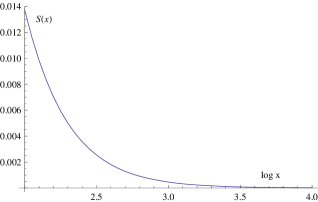
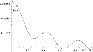
($c$)   ($d$)

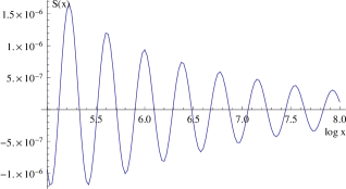
Figure 1: The graph of $S(x)\equiv S_{2,1}(x)$ against $\log_{10}x$ for different ranges of $x$.

The successive maxima ($x_{k}^{+}$) and minima ($x_{k}^{-}$) in the oscillatory region are determined by calculating the zeros of the derivative $S_{2,1}^{\prime}(x)$, where

$$S_{2,1}^{\prime}(x)=\sum_{n=1}^{\infty}\frac{\mu(n)}{n^{3}}\,e^{-X_{n}}=\frac{1}{\zeta(3)}-\sum_{n=1}^{\infty}\frac{\mu(n)}{n^{3}}\,(1-e^{-X_{n}}),$$

by using (2.10) with $p=3$. The results of these calculations together with the corresponding values of $S(x_{k}^{\pm})$ are shown in Table 1. Plots of $\log\,S_{2,1}(x_{k}^{\pm})$ against $\log\,x$ are shown in Fig. 2, where it is seen that they reveal a linear variation to a good approximation. The dashed lines in these figures have slope equal to $-0.25$, thereby numerically confirming the estimate in (1.2).

Table 1: Values of the maxima and minima $\log_{10}x_{k}^{\pm}$ and the corresponding values of $S_{2,1}(x_{k}^{\pm})$.

$k$	$\log_{10}x_{k}^{+}$	$S_{2,1}(x_{k}^{+})$	$\log_{10}x_{k}^{-}$	$S_{2,1}(x_{k}^{-})$
1	4.83284	$2.62044\times 10^{-6}$	4.65573	$-4.78520\times 10^{-7}$
2	5.22278	$1.65298\times 10^{-6}$	5.03476	$-1.20507\times 10^{-6}$
3	5.61033	$1.21568\times 10^{-6}$	5.41918	$-1.18328\times 10^{-6}$
4	5.99669	$9.38573\times 10^{-7}$	5.80406	$-1.00735\times 10^{-6}$
5	6.38315	$7.47310\times 10^{-7}$	6.19039	$-8.20165\times 10^{-7}$
6	6.76905	$5.93349\times 10^{-7}$	6.57596	$-6.62603\times 10^{-7}$
7	7.15545	$4.76797\times 10^{-7}$	6.96249	$-5.30007\times 10^{-7}$
8	7.54124	$3.80007\times 10^{-7}$	7.34817	$-4.26057\times 10^{-7}$

($a$)   ($b$)

Figure 2: Plots of (a) $\log_{10}S(x_{k}^{+})$ and (b) $\log_{10}S(x_{k}^{-})$ against $\log_{10}x$ (where $S(x)\equiv S_{2,1}(x)$). The dashed lines have slope $-0.25$.

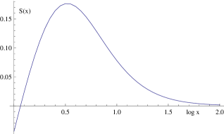
($a$)   ($b$)

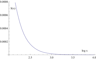
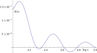
($c$)   ($d$)

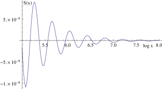
Figure 3: The graph of $S(x)\equiv S_{2,2}(x)$ against $\log_{10}x$ for different ranges of $x$.

The case of the original Riesz function has $m=p=2$ and from (2.1) we have

$$S_{2,2}(x)=\sum_{n=1}^{\infty}\frac{\mu(n)}{n^{2}}(1-e^{-X_{n}})-\frac{1}{\zeta(2)},$$

where $\zeta(2)=\pi^{2}/6$. The results are shown in Fig. 3 for the range $0\leq x\leq 10^{8}$ obtained using the scheme (2.10) with $p=2$. This function presents a similar behaviour with its value decreasing until about $10^{-8}$ before commencing to oscillate about the zero line. The first zero has the value $x\doteq 1.15671$. A plot of $xS_{2,2}(x)$ is also given in [2]. The successive maxima and minima in the oscillatory region are computed as the zeros of the derivative

$$S_{2,2}^{\prime}(x)=\frac{1}{\zeta(4)}-\sum_{n=1}^{\infty}\frac{\mu(n)}{n^{4}}(1-e^{-X_{n}}).$$

The results of these calculations together with the corresponding values of $S(x_{k}^{\pm})$ are shown in Table 2. Plots of $\log\,S_{2,2}(x_{k}^{\pm})$ against $\log\,x$ are shown in Fig. 4, where it is seen that they reveal a linear variation to a good approximation. The dashed lines in these figures have slope equal to $-0.75$, thereby numerically confirming the estimate in (1.2).

Table 2: Values of the maxima and minima $\log_{10}x_{k}^{\pm}$ and the corresponding values of $S_{2,2}(x_{k}^{\pm})$.

$k$	$\log_{10}x_{k}^{+}$	$S_{2,2}(x_{k}^{+})$	$\log_{10}x_{k}^{-}$	$S_{2,2}(x_{k}^{-})$
1	4.48752	$4.97204\times 10^{-8}$	4.31797	$-6.46896\times 10^{-9}$
2	4.87969	$1.97351\times 10^{-8}$	4.69479	$-1.67414\times 10^{-8}$
3	5.26779	$9.09065\times 10^{-9}$	5.07699	$-1.09071\times 10^{-8}$
4	5.65449	$4.53355\times 10^{-9}$	5.46263	$-5.99878\times 10^{-9}$
5	6.04080	$2.28418\times 10^{-9}$	5.84775	$-3.14719\times 10^{-9}$
6	6.42706	$1.17580\times 10^{-9}$	6.23435	$-1.62554\times 10^{-9}$
7	6.81307	$5.98676\times 10^{-10}$	6.61979	$-8.37753\times 10^{-10}$
8	7.19932	$3.07392\times 10^{-10}$	7.00651	$-4.29573\times 10^{-10}$

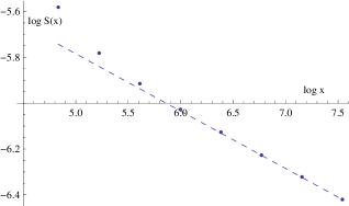
($a$)   ($b$)

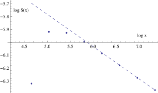
Figure 4: Plots of (a) $\log_{10}S(x_{k}^{+})$ and (b) $\log_{10}S(x_{k}^{-})$ against $\log_{10}x$ (where $S(x)\equiv S_{2,2}(x)$). The dashed lines have slope $-0.75$.

It has been shown in [1] that $S_{2,2}(x)$ has an infinite number of zeros. It is very probable that $S_{2,1}(x)$ also has an infinite number of zeros.

4. An asymptotic expansion

An integral representation of $S_{m,p}(x)$ in the form of a Mellin-Barnes integral is given by

$$S_{m,p}(x)=-\frac{1}{2\pi i}\int_{c-\infty i}^{c+\infty i}\frac{\Gamma(s)x^{-s}}{\zeta(p-ms)}\,ds\qquad(0<c<c_{0}),$$ (4.1)

where $c_{0}=(p-\mbox{${\textstyle\frac{1}{2}}$})/m$. The integrand possesses simple poles at $s=0,-1-2,\ldots$ and at the trivial zeros of the zeta function at $s=(p+2k)/m$, $k=1,2,\ldots\,$. On the assumption of the Riemann hypothesis, there is also an infinite number of (simple) poles on the line $\Re(s)=c_{0}$ given by $s=c_{0}\pm i\gamma_{k}/m$ ($k=1,2,\ldots$), where $\zeta(\mbox{${\textstyle\frac{1}{2}}$}\pm i\gamma_{k})=0$. Assuming that it is permissible to displace the integration path past this line, we obtain the result

$$S_{m,p}(x)=-\frac{2x^{-c_{0}}}{m}\Re\sum_{k=1}^{\infty}\frac{\Gamma(c_{0}-i\gamma_{k}/m)}{\zeta^{\prime}(\mbox{${\textstyle\frac{1}{2}}$}+i\gamma_{k})}\ x^{i\gamma_{k}/m}+O(x^{-(p+2)/m})$$

as $x\to+\infty$. The details of the case $m=2$, $p=1$ are discussed in [3, §2.5]; see also the account presented in [7, p. 143].

If we now set

$$A_{k}=\frac{\Gamma(c_{0}-i\gamma_{k}/m)}{\zeta^{\prime}(\mbox{${\textstyle\frac{1}{2}}$}+i\gamma_{k})},\qquad\psi_{k}=\pi+\arg A_{k},$$

we find that

$$S_{m,p}(x)=\frac{2x^{c_{0}}}{m}\sum_{k=1}^{\infty}|A_{k}|\cos\biggl{\{}\frac{\gamma_{k}}{m}\,\log\,x+\psi_{k}\biggr{\}}+O(x^{-(p+2)/m}).$$ (4.2)

The convergence of the sum (4.2) is difficult to establish. The gamma function present in the coefficients $A_{k}$ decays very rapidly for increasing $k$, since from Stirling’s formula it contains the exponential factor $\exp\,[-\pi\gamma_{k}/(2m)]$ for large $\gamma_{k}$. The magnitude of $\zeta^{\prime}(\mbox{${\textstyle\frac{1}{2}}$}+i\gamma_{k})$ (which is non-zero on the assumption that the non-trivial zeros are all simple) generally increases with $k$, but it is possible that there are zeros for which this quantity could become small.

When $m=p=2$, we obtain the expansion

$$S_{2,2}(x)=x^{-3/4}\sum_{k=1}^{\infty}|A_{k}|\cos\,\biggl{\{}\frac{\gamma_{k}}{2}\,\log\,x+\psi_{k}\biggr{\}}+O(x^{-2})$$ (4.3)

with $A_{k}=\Gamma(\mbox{${\textstyle\frac{3}{4}}$}-\mbox{${\textstyle\frac{1}{2}}$}i\gamma_{k})/\zeta^{\prime}(\mbox{${\textstyle\frac{1}{2}}$}+i\gamma_{k})$. The graph of $S_{2,2}(x)$ against $\log_{10}x$ compared with the expansion (4.3) truncated after $k=5$ terms is shown in Fig. 5. It is seen that for $x\,\raisebox{-3.44444pt}{\mbox{$\stackrel{{\scriptstyle\textstyle>}}{{\sim}}$}}\,10^{6}$ the curves are indistinguishable on the scale of the figure.

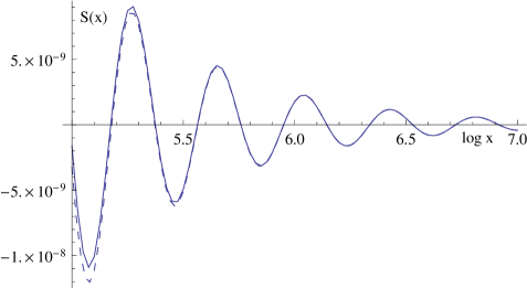
Figure 5: The graph of $S(x)\equiv S_{2,2}(x)$ against $\log_{10}x$ compared with the asymptotic form (4.3) (dashed curve).

5. Concluding remarks

The numerical results obtained in Section 3 are indicative only. It appears from the numerical investigation – without any reference to the Riemann hypothesis – that the large-$x$ behaviour of the functions $S_{2,1}(x)$ and $S_{2,2}(x)$ possesses respectively the $x^{-1/4}$ and $x^{-3/4}$ decay superimposed on an oscillatory structure. A striking feature of the plots in Figs. 1 and 3 is the fact that the final decaying oscillatory structure is not obtained until $x$ has attained the value of approximately $10^{5}$. This is an unusual occurrence since most special functions begin to exhibit their asymptotic structure for often surprisingly modest values of the variable.

The computation of $S_{m,p}(x)$ for $m\geq 3$ is made easier since the cut-off value $N$ then scales like $x^{1/m}$ and the rate of decay of the various series in (2.10) is correspondingly more rapid. As an example, the case $m=3$, $p=2$ is shown in [5]. The behaviour is found to be similar to that depicted in Figs, 1 and 3, with the maxima and minima following an approximate $x^{-1/2}$ scaling predicted by (4.2).

Appendix:  Derivation of Lemma 1

From the contiguous relation satisfied by the confluent hypergeometric function ${}_{1}F_{1}(a;b,z)$ [4, (13.3.2)]

$$b(b-1){}_{1}F_{1}(a;b-1;z)+b(1-b-z){}_{1}F_{1}(a;b;z)+z(b-a){}_{1}F_{1}(a;b+1;z)=0,$$

we obtain, with $a=1$, $b=k+2$, the recursion formula satisfied by $f_{k}(z):=e^{-z}{}_{1}F_{1}(1;k+1;z)$ in the form

$$f_{k}(z)-\biggl{(}1+\frac{z}{k+1}\biggr{)}f_{k+1}(z)+\frac{z}{k+2}f_{k+2}(z)=0\qquad(k\geq 0).$$

Repeated use of this result, combined with $f_{0}(z)=1$ and the partial sum of the exponential series $e_{k}(z)$ defined in (2.5), shows successively that

$$f_{1}(z) = \frac{1}{e_{2}(z)}+\frac{ze_{1}(z)}{2e_{2}(z)}\,f_{2}(z),$$

$$f_{2}(z) = \frac{1}{e_{3}(z)}+\frac{ze_{2}(z)}{3e_{3}(z)}\,f_{3}(z),$$

and, in general,

$$f_{k-1}(z)=\frac{1}{e_{k}(z)}+\frac{ze_{k-1}(z)}{ke_{k}(z)}\,f_{k}(z)\qquad(k\geq 1).$$ (A.1)

Then, from (A.1) we find that

$$zf_{1}(z) = \frac{z}{e_{2}(z)}+\frac{z^{2}f_{2}(z)}{2e_{2}(z)}=1-\frac{1}{e_{2}(z)}+\frac{z^{2}f_{2}(z)}{2e_{2}(z)}$$

$$= 1-\frac{1}{e_{2}(z)}+\frac{z^{2}}{2e_{2}(z)}\biggl{(}\frac{1}{e_{3}(z)}+\frac{ze_{2}(z)}{3e_{3}(z)}\,f_{3}(z)\biggr{)}$$

$$= 1-\frac{1}{e_{3}(z)}+\frac{z^{3}f_{3}(z)}{3!e_{3}(z)},$$

where we have used $e_{1}(z)=1$, $e_{2}(z)=1+z$ and have written $z^{2}/2!=e_{3}(z)-e_{2}(z)$. This procedure can be continued to produce the final result

$$zf_{1}(z)=1-\frac{1}{e_{k}(z)}+\frac{z^{k}f_{k}(z)}{k!e_{k}(z)}\qquad(k\geq 1).$$ (A.2)