Digitized-counterdiabatic quantum approximate optimization algorithm

Abstract

The quantum approximate optimization algorithm (QAOA) has proved to be an effective classical-quantum algorithm serving multiple purposes, from solving combinatorial optimization problems to finding the ground state of many-body quantum systems. Since QAOA is an ansatz-dependent algorithm, there is always a need to design ansatze for better optimization. To this end, we propose a digitized version of QAOA enhanced via the use of shortcuts to adiabaticity. Specifically, we use a counterdiabatic (CD) driving term to design a better ansatz, along with the Hamiltonian and mixing terms, enhancing the global performance. We apply our digitized-counterdiabatic QAOA to Ising models, classical optimization problems, and the $P$-spin model, demonstrating that it outperforms standard QAOA in all cases we study.

I Introduction

Hybrid classical-quantum algorithms have the potential to unleash a broad set of applications in the quantum computing realm. The challenges involved in realizing fault-tolerant quantum computer have promoted the study of such hybrid algorithms, which proved to be relevant to modern noisy intermediate-scale quantum (NISQ) devices [1, 2] with few hundred qubits and limited coherence time. One notable example is that of variational quantum algorithms (VQA), which is implemented by designing variational quantum circuits to minimize the expectation value for a given problem Hamiltonian. VQA is advantageous given the fact that preparing a tunable circuit ansatz is found to be difficult on a classical computer. It has already been widely applied in quantum chemistry [3, 4, 5, 6, 7, 8], condensed matter physics [9, 10, 11], solving linear system of equations [12], combinatorial optimization problems [13, 14] and several others [15, 16]. Remarkably, one of the early implementations of the VQA was performed using photonic quantum processors [17], which prompted further theoretical progress [18, 19, 20, 21, 22, 23]. VQA has been demonstrated in superconducting qubits [18, 3, 6] and trapped ions [8, 24, 25].

One compelling outcome of VQA is the development of the quantum approximate optimization algorithm (QAOA) [26], which provides an alternative for solving combinatorial optimization problems using shallow quantum circuits with classically optimized parameters. In the past few years, there has been a rapid development in QAOA-based techniques that have been applied not only for solving conventional optimization problems like MaxCut but also for solving ground state problems in different physical systems [27, 28, 25]. Improved versions of QAOA, like ADAPT-QAOA [29] and Digital-Analog QAOA [30] have also been reported recently. Like any combinatorial optimization problem, QAOA depends on optimizing a cost function to obtain the desired optimal state corresponding to a $p$-level parametrized quantum circuit. In addition, the choice of the approximate trial state, from which the cost function is obtained, is crucial to the success of the QAOA algorithm. Generally, this is done by using quantum adiabatic algorithms (QAA) which produce near-optimal results for large $p$ which is not suitable for current NISQ devices. Moreover, due to the requirement of large $p$, the cost of classical optimization increases and the algorithms suffer from the problem of vanishing gradients and local minima [31, 32, 33].

Several studies have been reported in past few years showing that high fidelity quantum states can be prepared by assisting QAA with additional driving interaction [34]. These studies establish that for certain problems, the inclusion of additional driving terms can reduce the computational complexity, and with it the circuit depth. These driving terms are usually calculated using methods developed under the umbrella of so-called shortcuts to adiabaticity  [35, 36], which have been introduced to improve the traditional quantum adiabatic processes, removing the requirement for slow driving [37]. Instances of these methods include counterdiabatic (CD) driving [38, 39, 40], fast-forward approach [41, 42], and invariant-based inverse engineering [43, 44]. Among them, CD driving is interesting and has been used to study fast dynamics [45, 46, 47, 48, 49], preparation of entangled states [50, 51, 52, 53], adiabatic quantum computing [54, 34] and quantum annealing [55, 56, 57].

In the context of QAOA, the advantage of the introduction of CD driving is twofold. The CD driving decreases the circuit depth, while reducing the number of optimization parameters. On the other hand, it provides a better approximate trial state which is beneficial for finding the optimal target state. In this work, we propose a novel algorithm, digitized-counterdiabatic quantum approximate optimization algorithm (DC-QAOA), which improves the performance of the conventional QAOA using CD driving. In this context, it is worthwhile to mention the work of Ref. [58], also inspired by CD driving techniques.

This article is organized as follows. In Sec. II, we introduce DC-QAOA algorithm and explain it in detail, comparing it with the quantum adiabatic evolution and QAOA. In the following sections we present a comparative study of the proposed DC-QAOA and the conventional QAOA method in the context of various physical systems. In Sec. III, we prepared the ground state of three different types of 1D Ising spin models, namely, the Longitudinal field Ising model (LFIM), the transverse field Ising model (TFIM), and the GHZ state. In Sec. IV, we studied classical optimization problems such as the MaxCut problem and the Sherrington-Kirkpatrick model, while in Sec. V, different variants of $P$-spin model are considered. In doing so, we establish, by comparing the approximation ratios, that the DC-QAOA is advantageous compared to the QAOA for shallow quantum circuits. We conclude with a discussion in Sec. VI.

II Digitized counter-diabatic quantum approximate optimization algorithm (DC-QAOA)

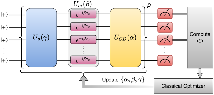
Figure 1: Schematic diagram with circuit used for DC-QAOA having additional CD term along with the Hamiltonian and mixing terms.

The conventional QAOA method can be viewed as a combination of two distinct parts: the quantum part consists of a parameterized circuit ansatz, which is in turn complemented by a classical optimization algorithm to determine the parameters that minimize (maximize) a predefined cost function. The circuit ansatz for the quantum part is governed by an annealing Hamiltonian,

$$H_{a}(t)=(1-\lambda(t))H_{mixer}+\lambda(t)H_{prob},$$ (1)

where $\lambda(t)\in[0,1]$ is the annealing schedule for $t\in[0,T]$. $H_{mixer}=\sum_{i}h_{i}\sigma^{x}_{i}$ is the mixing Hamiltonian that produces an equal (weighted) superposition state in the computational basis to begin with, whereas the desired final state is the ground state (or an eigenstate) of $H_{prob}$. In continuous annealing, the system evolves from the eigenstate of $H_{mixer}$ to the eigenstate of $H_{prob}$ through adiabatic evolution. The corresponding digital adiabatic circuit ansatz can be designed using the trotterized time evolution operator [59, 60]

$$U(0,T)\approx\prod_{j=1}^{p}\prod_{m=1}^{M}\exp\left\{-iH_{m}(j\Delta t)\Delta t\right\},$$ (2)

where we consider that $H_{a}(t)$ can be decomposed into $M$ $k$-local terms, i.e., into terms $H_{m}(t)$ which have $k$-body interactions at most. Note that the $U(0,T)$ is a product of $p$ sub-unitaries, each corresponding to an infinitesimal propagation step $\Delta t$. An adiabatic evolution using $U(0,T)$ can always produce an exact target state at the cost of resorting to a large value of $p$. This can be translated to the language of QAOA if one parameterizes $U(0,T)$ as

$$U(\bm{\gamma},\bm{\beta})=U_{m}{(\beta_{p})}U_{p}{(\gamma_{p})}U_{m}{(\beta_{p-1})}U_{p}{(\gamma_{p-1})}\dots U_{m}{(\beta_{1})}U_{p}{(\gamma_{1})},$$ (3)

where the evolution operators are $U_{m}{(\beta_{p})}=\exp{(-i\beta_{p}H_{mixer})}$ and $U_{p}{(\gamma_{p}})=\exp{(-i\gamma_{p}H_{prob})}$. Here, the annealing schedule is characterized by the discrete set of parameters $\{\beta_{p},\beta_{p-1},\dots,\beta_{1}\}$ and $\{\gamma_{p},\gamma_{p-1},\dots,\gamma_{1}\}$. $(\bm{\gamma},\bm{\beta})$ defines a $2p$ parameter space that corresponds to the depth of the circuit ansatz and the cost function $F(\bm{\gamma},\bm{\beta})$ is optimized classically to obtain an optimal parameter set $(\bm{\gamma}^{*},\bm{\beta}^{*})$, which produces the desired target state, i.e., $\ket{\psi(\bm{\gamma}^{*},\bm{\beta}^{*}})$. Note that in most cases this target state is chosen to be the ground state of $H_{prob}$.

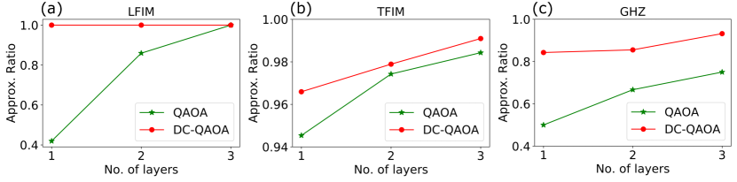
Figure 2: Comparison of approximation ratios ($\mathcal{R}$) as a function of number of layers ($p$) for three representative cases of Ising spin model. Green lines show results of QAOA whereas red lines show results of DC-QAOA. (a) shows $\mathcal{R}$ variation of LFIM where $J_{ij}=1$, $h_{i}=1$, and $k_{i}=0$. (b) depicts TFIM where $J_{ij}=1$, $h_{i}=0$, and $k_{i}=1$, and (c) shows preparation of GHZ state where $J_{ij}=1$, $h_{i}=0$, and $k_{i}=0$. System size for all the cases was kept to $L=12$ qubits.

As the case of adiabatic evolution, QAOA requires large $p$ to obtain a near-optimal trial state, even with the assistance of the classical optimizer. In addition, the realization of $U(\bm{\beta},\bm{\gamma})$ for an interacting many-body system for large $p$ becomes inefficient due to the large number of gates involved. In DC-QAOA, we focus on improving the quantum part of QAOA, by adding a variational parameter in each step, i.e.,

$$U(\bm{\gamma},\bm{\beta})\rightarrow U(\bm{\gamma},\bm{\beta},\bm{\alpha}),\;\;\;F(\bm{\gamma},\bm{\beta})\rightarrow F(\bm{\gamma},\bm{\beta},\bm{\alpha}),$$ (4)

The application of another parameter decreases the size of $p$ drastically. This additional parameter can be quantified as the inclusion of the CD driving term in the problem Hamiltonian. The resulting circuit ansatz is shown in Fig. 1.

In general, CD driving amounts to using an additional control Hamiltonian in Eq. (1), required for suppressing non-adiabatic transitions [61, 38, 39, 40]. This is especially effective for many-body systems with tightly spaced eigenstates. CD driving comes at a cost, as it generally involves nonlocal many-body interactions, and their exact specification of the CD Hamiltonian term requires access to the spectral properties of the driven system [38, 40, 45]. As a way out, variational approximations have been proposed to obtain the CD terms [50, 62, 63]. In this context, one can use the adiabatic gauge potential for finding an approximate CD driving without spectral information of the system [63, 64].

In the following sections, a pool of CD operators is defined using the nested commutator approach of the adiabatic gauge potential, provided by Claeys et. al. [65],

$$A_{\lambda}^{(l)}=i\sum_{k=1}^{l}\alpha_{k}(t)\underbrace{[H_{a},[H_{a},......[H_{a},}_{2k-1}\partial_{\lambda}H_{a}]]].$$ (5)

Here we considered up to the second order in the expansion of the nested commutator, $l=2$, which gives rise to an operator pool $A=\{\sigma^{y},\sigma^{z}\sigma^{y},\sigma^{y}\sigma^{z},\sigma^{x}\sigma^{y},\sigma^{y}\sigma^{x}\}$, including solely local and two-body interactions. Note that the choice of this operator pool depends on $H_{a}(t)$ and may contain other operators depending on the problem Hamiltonian. However, $A$ contains every possible CD operator that can be derived from the problem Hamiltonians, used in the present study. We chose the CD term as a combination of these operators for each system based on the success probability of the algorithm. For instance, the local CD driving term provides better success probability in the case of the transverse-field Ising model and $P$-spin model, however not suitable for solving the MaxCut Hamiltonian. The CD coefficients $\alpha_{k}$ are transformed into the additional variational parameter associated with the CD driving. The addition of such a new free parameter increases the degrees of freedom, making it possible to reach broader parts of the Hilbert space of the Hamiltonian with a lower circuit depth than in QAOA. Furthermore, as DC-QAOA only requires the operator form of the CD driving combined with the additional set of parameters $\bm{\alpha}$, it eliminates the requirement of complex calculation of the CD coefficients. DC-QAOA is also more flexible in regards to the boundary conditions compared to the CD evolution which permits the application of the driving term even for one step only. Moreover, the operators can be chosen heuristically and according to the requirement of the system which is being studied.

Although there are several ways to define the cost function, we opt for the most convenient one which is the energy expectation value of the problem Hamiltonian calculated for the trial wave function,

$$F(\bm{\gamma},\bm{\beta},\bm{\alpha})=\bra{\psi(\bm{\gamma},\bm{\beta},\bm{\alpha})}H_{prob}\ket{\psi(\bm{\gamma},\bm{\beta},\bm{\alpha})},$$ (6)

where $\psi(\bm{\gamma},\bm{\beta},\bm{\alpha})$ represents the approximate trial state produced by the digitized CD ansatz. The efficiency of our algorithm can be measured in terms of the approximation ratio, given by,

$$\mathcal{R}=\frac{F(\bm{\gamma},\bm{\beta},\bm{\alpha})}{{E_{0}}},$$ (7)

where $E_{0}$ is the ground state energy of the system.

Classical optimization techniques are an integral part of variational algorithms, which helps to find the optimal parameters that minimize the cost function. Our work mainly considers two optimization techniques, namely Momentum Optimizer and Adagrad Optimizer, which are specific examples of stochastic gradient descent (SGD) algorithms. Momentum Optimizer is a variant of SGD in which a momentum term is added along with the gradient descent. The prime purpose of the momentum term is to increase the parameter update rate when gradients are in the same direction and decrease the update rate when gradients point in a different direction [66]. On the other hand, Adagrad Optimizer’s main purpose is to change the update rate based on the past descent results [67]. Adagrad has shown great improvements in the robustness of SGD [68]. These two classical optimization techniques work pretty well for the cases we consider. This is because these optimization routines have proven faster convergence than gradient descent. Moreover, some of the cases we study involve a large Hilbert space, which may lead to local minima in the energy landscape. In the presence of steep gradients, the use of these techniques proves beneficial. This problem dependence of the performance is shared with other optimization routines such as Nesterov Momentum, Adam, and AdaMax. An overview and comparison about challenges faced by the different types of gradient descent optimization, can be found in Ref. [69].

III Ising spin Models

1D quantum Ising spin chains are the manifestation of the simplest many-body systems that are widely studied in existing quantum processors. Numerous computational problems can be mapped to finding the ground state of the Ising-like Hamiltonians, which makes it suitable for benchmarking various quantum algorithms. The general form of the Hamiltonian of 1D Ising spin model is given by,

$$H_{prob}(\sigma)=-\displaystyle\sum_{<i,j>}J_{ij}\sigma_{i}^{z}\sigma_{j}^{z}-\displaystyle\sum_{i}h_{i}\sigma_{i}^{z}-\displaystyle\sum_{i}k_{i}\sigma_{i}^{x},$$ (8)

where $\sigma_{i}^{\delta}$ denotes the Pauli matrices at the $i$th site, and $<i,j>$ corresponds to the nearest-neighbor interaction with strength $J_{ij}$. The on-site interaction terms $h_{i}$ and $k_{i}$ represent the longitudinal and transverse fields, respectively. We consider the periodic boundary conditions so that our model describes a ring of interacting spins [70, 71, 72]. Note that three special cases can be retrieved from Eq. (8): i) longitudinal field Ising model (LFIM) when $k_{i}=0$, ii) transverse field Ising model (TFIM) when $h_{i}=0$, and iii) a special case when both $k_{i}=0$ and $h_{i}=0$, for which the resulting ground state of $H_{prob}$ is the highly entangled Greenberger-Horne-Zeilinger (GHZ) state [73, 74, 75, 76]. For simplicity, we choose the system to be homogeneous i.e., $J_{ij}=J$ as well as $h_{i}=h_{z}$ and $k_{i}=h_{x}$. To prepare an equal superposition of the qubits, as a input of the circuit ansatz, the mixing Hamiltonian is chosen as $H_{mixer}=\sum_{i}\sigma_{i}^{x}$. To implement DC-QAOA, as mentioned in Sec. II, along with the problem and mixer Hamiltonian, we include the CD term to define the circuit ansatz. The CD operator is chosen heuristically from the operator pool $A$. For instance, in the case of LFIM, the ground state is ferromagnetic and constitutes a large energy gap with the first excited state for the chosen interaction strengths. In such cases, the local driving term $A_{t}=\sum_{i}\sigma^{y}_{i}$ can produce the ground state. On the other hand, the ground state of TFIM is closely spaced with the nearby excited states, which makes the local driving term insufficient. Similarly, the local driving term is also not suitable for GHZ state [61]. Instead, the second-order term $A_{t}=\sum_{i}\sigma^{z}_{i}\sigma^{y}_{i+1}$ is more likely to produce a better result. The unitary operator that represents the CD part of the circuit ansatz is given by,

$$U_{CD}(\alpha)=\prod_{j=1}^{L}e^{-i\alpha A_{t}^{q}},$$ (9)

where $A_{t}^{q}$ represents the respective $q$-local CD operator chosen from the CD pool $A$. For instance, if $q=1$ then $A_{t}^{q}=\{A_{t}\}_{j}$ and if $q=2$, then $A_{t}^{q}=\{A_{t}\}_{j,j+1}$. The circuit is designed using the gate model of quantum computing whereas the classical optimization is the stochastic gradient descent method. Fig. 2 depicts the improvement obtained by DC-QAOA over traditional QAOA. In the simulation, we study a $12$-qubit system, for which we compute $\mathcal{R}$ for different $p$ values. For LFIM, as shown in Fig. 2a, $\mathcal{R}=1$ even for $p=1$ with DC-QAOA which constitutes considerable improvement over QAOA, that requires $p=3$ to achieve unit $\mathcal{R}$. Hence, for Fig. 2a, the number of variational parameters required to achieve unit $\mathcal{R}=1$ for DC-QAOA is $3p=3$ whereas for QAOA it is $2p=6$. We also see that, for a lower number of layers i.e., $p=1,2,3$, DC-QAOA converges faster to the unit $\mathcal{R}$ compared to QAOA. Furthermore, while DC-QAOA shows better convergence at lower depths, for the TFIM and the GHZ states, the exact ground state can only be achieved with $p\geq L/2$ layers. This effect can be attributed to the Lieb-Robinson bound [77, 78] which forces the circuits for TFIM and GHZ state to scale linearly with the system size in order to achieve unit $\mathcal{R}$.

To compare the resource requirements, both classical and quantum, one can inspect two crucial elements of these methods. In the case of systems with nearest-neighbor interactions, the increase in circuit depth per layer by adding a CD term will be constant, and it depends on the CD term chosen. The circuit depth can be quantified as $d\times p$, and the CD driving increases it to $(d+d_{cd})\times p$, where $d_{cd}$ represents the increment in depth per layer. For LFIM, the CD term $\sigma_{y}$ gives $d_{cd}=1$, whereas for TFIM $d_{cd}=4$ for $\sigma_{z}\sigma_{y}$. On the other hand, the increase in parameter space due to the CD term is always from $2p$ to $3p$, making DC-QAOA advantageous specifically for low $p$ values. In the limit of large $p$, the performance of QAOA and DC-QAOA becomes comparable for fixed system size.

IV Classical Optimization problems

Thus far, we have discussed the applications of DC-QAOA for finding the ground state of the Ising model and preparing entangled states. Combinatorial optimization problems are another set of problems that can be encoded in the ground state of a quantum Hamiltonian, diagonal in the computational basis. Here we discuss the application of DC-QAOA for solving combinatorial optimization problems, where the main objective is to find the optimal solution for a given classical cost function. MaxCut is one fundamental combinatorial optimization problem that has been solved using QAOA.

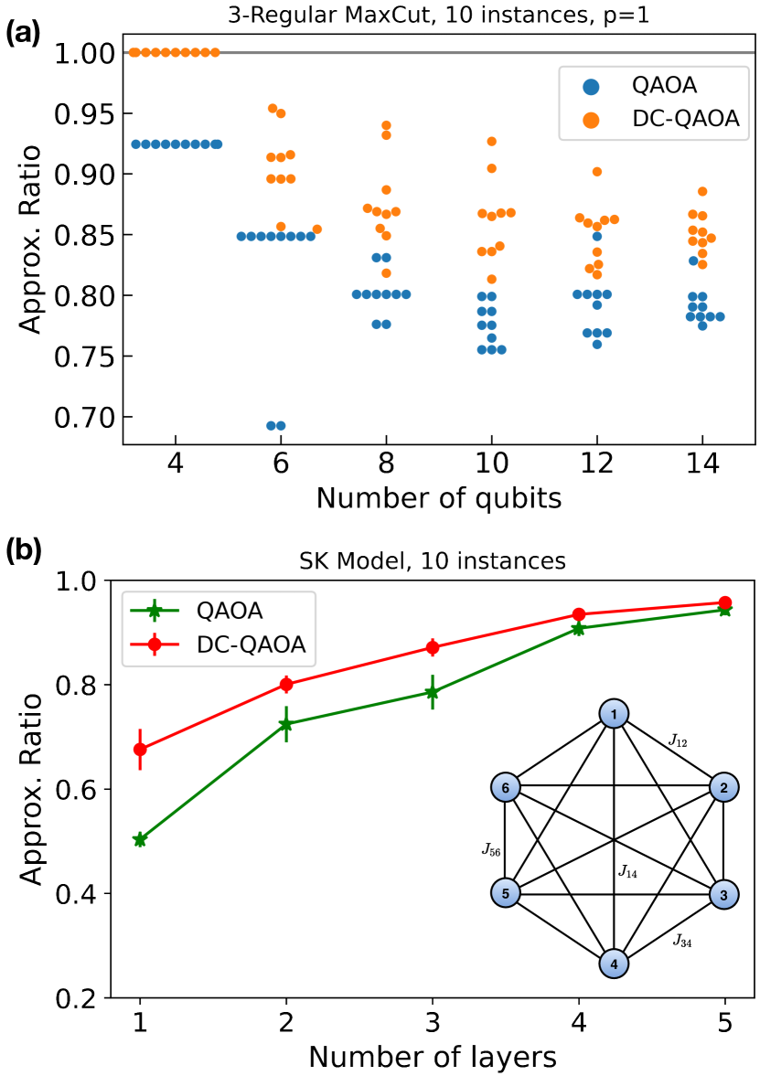
Figure 3: Comparison of approximation ratios obtained for different graph size using DC-QAOA and QAOA. (a) Unweighted 3-regular MaxCut for a randomly chosen 10 instances. (b) Approximation ratio vs number of layers ($p$) for SK model with 6-qubits (vertices) is depicted. Green line and red line show the values of QAOA and DC-QAOA respectively. On the right-bottom, a graph of 6 qubits with all-to-all connectivity is also shown. The results were obtained by considering 10 different randomly chosen instances of $J_{ij}$ values. Error bars represents the standard error.

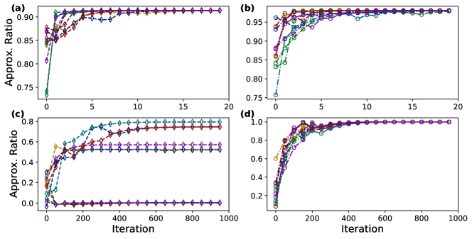
Figure 4: Comparison of approximation ratio ($\mathcal{R}$) with respect to number of iterations for $P=4$ and $p=1$. Panels (a) and (b) show the QAOA and DC-QAOA results for $h=1$, respectively. The case with $h=0$ is shown in panels (c) and (d) for QAOA and DC-QAOA results, respectively. The system size is $L=6$. Each of the 10 random initial parameters chosen is represented by a color line.

For the MaxCut problem, let us consider a graph $G=(V,E)$, where $V$ and $E$ being the vertex set and edge set respectively. We consider a classical cost function $C(z)$ defined on binary strings $\bm{z}=\left(z_{1},z_{2},\ldots,z_{n}\right)$, and aim at separating the vertices into two sets so that the number of edges cut by $C(z)$ is maximized. This maximizes the classical cost function

$$C(z)=\frac{1}{2}\sum_{(i,j)\in E}w_{ij}(1-z_{i}z_{j}),$$ (10)

where $w_{ij}$ represents the edge weight between vertices $i$ and $j$. Depending on the sets that the vertices of each edge are in after the cut, binary values (either $0$ or $1$) are assigned to variables $z_{i}$ and $z_{j}$ corresponding to respective vertices. This situation can be encoded in the ground state of the problem Hamiltonian by mapping the binary variables to Pauli operators

$$H(\sigma)=\displaystyle\sum_{(i,j)\in E}J_{ij}\sigma_{i}^{z}\sigma_{j}^{z}.$$ (11)

Note that Eq. (11) also belongs to the Ising class and is equivalent to Eq. (8) for GHZ states if only nearest neighbor interaction is considered, which is the case of the $2$-regular MaxCut. Here, to verify the performance of our algorithm, we consider unweighted ($w_{ij}=J_{ij}=1$) $3$-regular MaxCut problem, with each vertex connected to three other vertices. The CD operator pool can be obtained from the NC expansion and is given by $A=\{\sigma^{z}\sigma^{y},\sigma^{y}\sigma^{z}\}$. In Fig. 3 (a), the approximation ratio $\mathcal{R}$ for different graph sizes with up to 14 vertices (qubits) are shown for a single layer ($p=1$). We notice that for small graph sizes, say $4$ qubits), DC-QAOA is superior as it reaches unit $\mathcal{R}$. However, for a bigger graph $\mathcal{R}$ decreases gradually while exceeding the performance of QAOA. Although this can be improved for $p>1$ but for large depth DC-QAOA, the number of parameters for each step scales as $3p$, so the landscape of the cost function most likely has a complicated form, and we expect to see the problem of vanishing gradients (Barren plateau). A detailed analysis is needed for $p>1$ DC-QAOA, which we leave for future work.

Interestingly, if $J_{ij}$ is chosen as random all-to-all two-body interactions, Eq. (11) represents the so-called Sherrington-Kirkpatrick (SK) model. SK model is a classical spin model proposed by Sherrington and Kirkpatrick [79, 80] where $J_{ij}$ are interaction terms such that $J=\{\forall J_{ij}\}$ has zero mean and unit variance. For instance, they can be randomly chosen from the set $J=\{-1,1\}$ with probability $1/2$. The SK model is interesting for DC-QAOA as it can be studied as a combinatorial search problem on a complete graph. QAOA on the SK model has been extensively studied recently [81, 82]. Here, ten different instances of $J_{ij}$ values are considered in a system of $L=6$ spins. Note that the couplings $J_{ij}$ are non-uniform and the CD term depends on the choice of $J_{ij}$. As this model involves similar interactions to that in the MaxCut problem, we chose the CD term from the same operator pool, $A=\{\sigma^{z}\sigma^{y},\sigma^{y}\sigma^{z}\}$, calculated from the nested commutator ansatz. In fact, the CD-term chosen for the SK model is $A_{t}=J_{ij}\sigma_{i}^{z}\sigma_{j}^{y}$, where the operators are applied to all the sites due to its all-to-all connectivity.

In Fig. 3b, the approximation ratio ($\mathcal{R}$) is shown with respect to a varying number of layers ($p$). We observe that $\mathcal{R}$ is higher for DC-QAOA as compared to QAOA and that as the number of layers increases DC-QAOA and QAOA start to converge to the same value. This shows that DC-QAOA is efficient for instances where the circuit ansatz is low-layered. In fact, for low layers, although not giving the exact ground state DC-QAOA gives significantly enhanced $\mathcal{R}$. This could be advantageous as we can find optimal parameters which could be used as initial parameters for high-layered QAOA.

V $P$-spin Model

As a final benchmark, we consider the $P$-spin model, which is a long-range exactly-solvable fully-connected model  [83, 84, 85, 86]. The system Hamiltonian reads

$$H=-\frac{1}{L^{P-1}}\left(\sum_{i=1}^{L}\sigma^{z}_{i}\right)^{P}-h\sum_{i=1}^{L}\sigma^{x}_{i}$$ (12)

While the ground-state of Hamiltonian (12) is trivial, the presence of a quantum phase transition makes its preparation challenging by quantum annealing [83]. For $P=2$ this Hamiltonian exhibits a second-order phase transition whereas a first-order phase transition occurs for $P\geq 3$, closing the energy gap exponentially with increasing system size. This has motivated proposals to change the first-order phase into second-order phase transition by making the Hamiltonian non-stoquastic [87, 88]. The nature of the ground state also depends on $P$. For odd $P$ the ground state is non-degenerate, while for even $P$ it has a two-fold degeneracy with $Z_{2}$ symmetry, which makes the choice of the CD operator difficult [57].

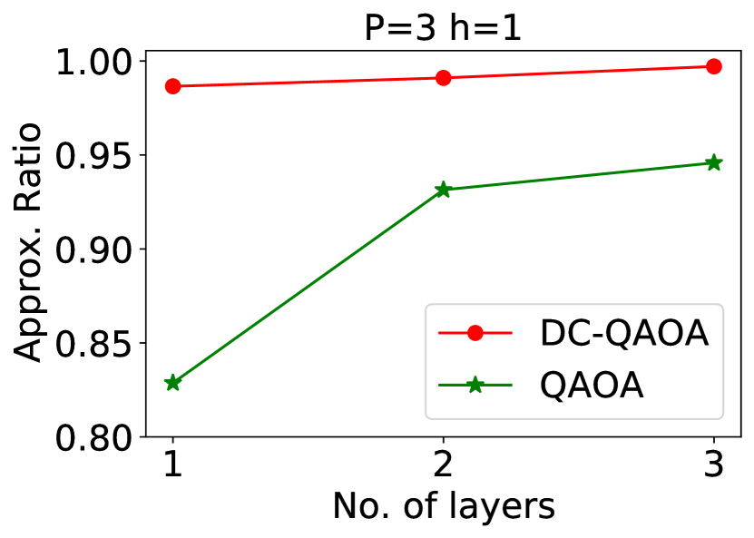
Figure 5: Approximation ratio ($\mathcal{R}$) as a function of number of layers ($p=1,2,3$) for $P=3$ and $h=1$. Green and red lines show the average results obtained from 10 random parameter initialization for QAOA and DC-QAOA, respectively. Standard deviations are of the order of $10^{-2}$.

We study DC-QAOA in a $6$ qubit $P$-spin model for the nontrivial case of $h\neq 0$ using local CD operator $A_{t}=\sum_{i}\sigma^{y}_{i}$. QAOA and DC-QAOA are compared for three different cases: $P=3$ , $h=1$ and $P=4$, $h=\{0,1\}$ respectively. Fig. 4 and Fig. 5 shows the advantage obtained by DC-QAOA for $P=4$ and $P=3$ respectively. For $P=4$, $\mathcal{R}$ as a function of number of iterations is shown for $p=1$ for $10$ random parameter initialization. We observe that for a finite number of iterations, DC-QAOA shows higher $\mathcal{R}$ values as compared to QAOA for both $h=0$ and $h=1$. It is evident that, in the case of $h=0$, QAOA is highly dependent on the choice of initial parameters and lands into local minima in some instances. By contrast, DC-QAOA shows unit $\mathcal{R}$ for every instance. For $P=3,h=1$, $\mathcal{R}$ is shown as a function of number of layers ($p=1,2,3$) for $10$ random initial parameters. As expected, for DC-QAOA, $\mathcal{R}$ values end up close to unity even for $p=1$ and $\mathcal{R}$ values increase as the number of layers increases. However, this is not surprising for $P=3$ as the ground state is a product state making it favorable for the local CD operator. The more intriguing case is in Fig. 4b, where the approximation ratio reaches close to unity for $p=1$ even when the ground state is degenerate. This occurs simply because the trial state converges to a particular one of the two due to the local CD driving. This is in contrast with QAOA, which does not achieve the target state for $p=1$ in any case.

VI Discussion and Conclusion

We have introduced a quantum algorithm leveraging the strengths of shortcuts to adiabaticity for quantum approximate optimization algorithms. Specifically, we have formulated a variant of QAOA using CD driving, called DC-QAOA, and established its enhanced performance over QAOA in finding ground states of different models. We benchmark our algorithm by considering various examples, starting with Ising spin models, preparing entangled states, classical optimization problems like MaxCut and SK model and, the P-spin model. Including the CD term to the circuit ansatz, the performance of the QAOA algorithm is enhanced. Results reveal that for low-layered circuits, DC-QAOA converges to the ground state faster than state-of-the-art QAOA. Thus, adding a new free parameter in the form of a gate chosen from a predefined set (CD term) increases the performance of the algorithm for shorter circuit depths. Thus, DC-QAOA turns out to be a preferable algorithm for circuits of shorter depth.

In conclusion, DC-QAOA outperforms QAOA for all the models we have studied. For high-depth circuits, DC-QAOA can be applied for initial layers only to enhance the performance of the standard QAOA. An interesting prospect would be to use the resulting optimal parameters from low depth DC-QAOA as the initial parameters of a high-depth QAOA in order to obtain the minima of the cost function efficiently. Our work shows that implementing principles of shortcuts-to-adiabaticity to enhance quantum algorithms has both fundamental and practical importance. The experimental realization of DC-QAOA on real hardware offers an exciting prospect for further progress.

Note: As we finished this work, we learned about the recent preprint devoted to QAOA assisted by CD  [89].

References

- Preskill [2018] J. Preskill, Quantum Computing in the NISQ era and beyond, Quantum 2, 79 (2018).
- Bharti et al. [2021] K. Bharti, A. Cervera-Lierta, T. H. Kyaw, T. Haug, S. Alperin-Lea, A. Anand, M. Degroote, H. Heimonen, J. S. Kottmann, T. Menke, W.-K. Mok, S. Sim, L.-C. Kwek, and A. Aspuru-Guzik, Noisy intermediate-scale quantum (nisq) algorithms (2021), arXiv:2101.08448 [quant-ph] .
- Colless et al. [2018] J. I. Colless, V. V. Ramasesh, D. Dahlen, M. S. Blok, M. E. Kimchi-Schwartz, J. R. McClean, J. Carter, W. A. de Jong, and I. Siddiqi, Computation of molecular spectra on a quantum processor with an error-resilient algorithm, Phys. Rev. X 8, 011021 (2018).
- Grimsley et al. [2019] H. R. Grimsley, S. E. Economou, E. Barnes, and N. J. Mayhall, An adaptive variational algorithm for exact molecular simulations on a quantum computer, Nature Communications 10, 3007 (2019).
- Cao et al. [2019] Y. Cao, J. Romero, J. P. Olson, M. Degroote, P. D. Johnson, M. Kieferová, I. D. Kivlichan, T. Menke, B. Peropadre, N. P. D. Sawaya, S. Sim, L. Veis, and A. Aspuru-Guzik, Quantum chemistry in the age of quantum computing, Chemical Reviews 119, 10856 (2019).
- Kandala et al. [2017] A. Kandala, A. Mezzacapo, K. Temme, M. Takita, M. Brink, J. M. Chow, and J. M. Gambetta, Hardware-efficient variational quantum eigensolver for small molecules and quantum magnets, Nature 549, 242 (2017).
- Nam et al. [2020] Y. Nam, J.-S. Chen, N. C. Pisenti, K. Wright, C. Delaney, D. Maslov, K. R. Brown, S. Allen, J. M. Amini, J. Apisdorf, K. M. Beck, A. Blinov, V. Chaplin, M. Chmielewski, C. Collins, S. Debnath, K. M. Hudek, A. M. Ducore, M. Keesan, S. M. Kreikemeier, J. Mizrahi, P. Solomon, M. Williams, J. D. Wong-Campos, D. Moehring, C. Monroe, and J. Kim, Ground-state energy estimation of the water molecule on a trapped-ion quantum computer, npj Quantum Information 6, 33 (2020).
- Hempel et al. [2018] C. Hempel, C. Maier, J. Romero, J. McClean, T. Monz, H. Shen, P. Jurcevic, B. P. Lanyon, P. Love, R. Babbush, A. Aspuru-Guzik, R. Blatt, and C. F. Roos, Quantum chemistry calculations on a trapped-ion quantum simulator, Phys. Rev. X 8, 031022 (2018).
- Cade et al. [2020] C. Cade, L. Mineh, A. Montanaro, and S. Stanisic, Strategies for solving the fermi-hubbard model on near-term quantum computers, Physical Review B 102 (2020).
- Endo et al. [2020] S. Endo, I. Kurata, and Y. O. Nakagawa, Calculation of the green’s function on near-term quantum computers, Physical Review Research 2 (2020).
- Bravo-Prieto et al. [2020a] C. Bravo-Prieto, J. Lumbreras-Zarapico, L. Tagliacozzo, and J. I. Latorre, Scaling of variational quantum circuit depth for condensed matter systems, Quantum 4, 272 (2020a).
- Bravo-Prieto et al. [2020b] C. Bravo-Prieto, R. LaRose, M. Cerezo, Y. Subasi, L. Cincio, and P. J. Coles, Variational quantum linear solver (2020b), arXiv:1909.05820 [quant-ph] .
- Liu et al. [2021] X. Liu, A. Angone, R. Shaydulin, I. Safro, Y. Alexeev, and L. Cincio, Layer vqe: A variational approach for combinatorial optimization on noisy quantum computers (2021), arXiv:2102.05566 [quant-ph] .
- Nannicini [2019] G. Nannicini, Performance of hybrid quantum-classical variational heuristics for combinatorial optimization, Physical Review E 99 (2019).
- Anschuetz et al. [2018] E. R. Anschuetz, J. P. Olson, A. Aspuru-Guzik, and Y. Cao, Variational quantum factoring (2018), arXiv:1808.08927 [quant-ph] .
- Karamlou et al. [2021] A. H. Karamlou, W. A. Simon, A. Katabarwa, T. L. Scholten, B. Peropadre, and Y. Cao, Analyzing the performance of variational quantum factoring on a superconducting quantum processor (2021), arXiv:2012.07825 [quant-ph] .
- Peruzzo et al. [2014] A. Peruzzo, J. McClean, P. Shadbolt, M.-H. Yung, X.-Q. Zhou, P. J. Love, A. Aspuru-Guzik, and J. L. O’Brien, A variational eigenvalue solver on a photonic quantum processor, Nature Communications 5, 4213 (2014).
- O’Malley et al. [2016] P. J. J. O’Malley, R. Babbush, I. D. Kivlichan, J. Romero, J. R. McClean, R. Barends, J. Kelly, P. Roushan, A. Tranter, N. Ding, B. Campbell, Y. Chen, Z. Chen, B. Chiaro, A. Dunsworth, A. G. Fowler, E. Jeffrey, E. Lucero, A. Megrant, J. Y. Mutus, M. Neeley, C. Neill, C. Quintana, D. Sank, A. Vainsencher, J. Wenner, T. C. White, P. V. Coveney, P. J. Love, H. Neven, A. Aspuru-Guzik, and J. M. Martinis, Scalable quantum simulation of molecular energies, Phys. Rev. X 6, 031007 (2016).
- McClean et al. [2016] J. R. McClean, J. Romero, R. Babbush, and A. Aspuru-Guzik, The theory of variational hybrid quantum-classical algorithms, New Journal of Physics 18, 023023 (2016).
- McClean et al. [2017] J. R. McClean, M. E. Kimchi-Schwartz, J. Carter, and W. A. de Jong, Hybrid quantum-classical hierarchy for mitigation of decoherence and determination of excited states, Phys. Rev. A 95, 042308 (2017).
- Barkoutsos et al. [2018] P. K. Barkoutsos, J. F. Gonthier, I. Sokolov, N. Moll, G. Salis, A. Fuhrer, M. Ganzhorn, D. J. Egger, M. Troyer, A. Mezzacapo, S. Filipp, and I. Tavernelli, Quantum algorithms for electronic structure calculations: Particle-hole hamiltonian and optimized wave-function expansions, Phys. Rev. A 98, 022322 (2018).
- Romero et al. [2018] J. Romero, R. Babbush, J. R. McClean, C. Hempel, P. J. Love, and A. Aspuru-Guzik, Strategies for quantum computing molecular energies using the unitary coupled cluster ansatz, Quantum Science and Technology 4, 014008 (2018).
- Lee et al. [2019] J. Lee, W. J. Huggins, M. Head-Gordon, and K. B. Whaley, Generalized unitary coupled cluster wave functions for quantum computation, Journal of Chemical Theory and Computation 15, 311 (2019).
- Shen et al. [2017] Y. Shen, X. Zhang, S. Zhang, J.-N. Zhang, M.-H. Yung, and K. Kim, Quantum implementation of the unitary coupled cluster for simulating molecular electronic structure, Phys. Rev. A 95, 020501 (2017).
- Pagano et al. [2020] G. Pagano, A. Bapat, P. Becker, K. S. Collins, A. De, P. W. Hess, H. B. Kaplan, A. Kyprianidis, W. L. Tan, C. Baldwin, L. T. Brady, A. Deshpande, F. Liu, S. Jordan, A. V. Gorshkov, and C. Monroe, Quantum approximate optimization of the long-range ising model with a trapped-ion quantum simulator, Proceedings of the National Academy of Sciences 117, 25396 (2020).
- Farhi et al. [2014] E. Farhi, J. Goldstone, and S. Gutmann, A quantum approximate optimization algorithm (2014), arXiv:1411.4028 [quant-ph] .
- Willsch et al. [2020] M. Willsch, D. Willsch, F. Jin, H. De Raedt, and K. Michielsen, Benchmarking the quantum approximate optimization algorithm, Quantum Information Processing 19 (2020).
- Wauters et al. [2020] M. M. Wauters, G. B. Mbeng, and G. E. Santoro, Polynomial scaling of qaoa for ground-state preparation of the fully-connected p-spin ferromagnet (2020), arXiv:2003.07419 [quant-ph] .
- Zhu et al. [2020] L. Zhu, H. L. Tang, G. S. Barron, F. A. Calderon-Vargas, N. J. Mayhall, E. Barnes, and S. E. Economou, An adaptive quantum approximate optimization algorithm for solving combinatorial problems on a quantum computer (2020), arXiv:2005.10258 [quant-ph] .
- Headley et al. [2020] D. Headley, T. Müller, A. Martin, E. Solano, M. Sanz, and F. K. Wilhelm, Approximating the quantum approximate optimisation algorithm (2020), arXiv:2002.12215 [quant-ph] .
- McClean et al. [2018] J. R. McClean, S. Boixo, V. N. Smelyanskiy, R. Babbush, and H. Neven, Barren plateaus in quantum neural network training landscapes, Nature Communications 9, 4812 (2018).
- Cerezo et al. [2021] M. Cerezo, A. Sone, T. Volkoff, L. Cincio, and P. J. Coles, Cost function dependent barren plateaus in shallow parametrized quantum circuits, Nature Communications 12 (2021).
- Grant et al. [2019] E. Grant, L. Wossnig, M. Ostaszewski, and M. Benedetti, An initialization strategy for addressing barren plateaus in parametrized quantum circuits, Quantum 3, 214 (2019).
- Hegade et al. [2021a] N. N. Hegade, K. Paul, Y. Ding, M. Sanz, F. Albarrán-Arriagada, E. Solano, and X. Chen, Shortcuts to adiabaticity in digitized adiabatic quantum computing, Phys. Rev. Applied 15, 024038 (2021a).
- Guéry-Odelin et al. [2019] D. Guéry-Odelin, A. Ruschhaupt, A. Kiely, E. Torrontegui, S. Martínez-Garaot, and J. G. Muga, Shortcuts to adiabaticity: Concepts, methods, and applications, Rev. Mod. Phys. 91, 045001 (2019).
- Torrontegui et al. [2013] E. Torrontegui, S. Ibáñez, S. Martínez-Garaot, M. Modugno, A. del Campo, D. Guéry-Odelin, A. Ruschhaupt, X. Chen, and J. G. Muga, Chapter 2 - shortcuts to adiabaticity, Advances In Atomic, Molecular, and Optical Physics 62, 117 (2013).
- Takahashi [2019] K. Takahashi, Hamiltonian engineering for adiabatic quantum computation: Lessons from shortcuts to adiabaticity, Journal of the Physical Society of Japan 88, 061002 (2019).
- Demirplak and Rice [2003] M. Demirplak and S. A. Rice, Adiabatic population transfer with control fields, The Journal of Physical Chemistry A 107, 9937 (2003).
- Demirplak and Rice [2005] M. Demirplak and S. A. Rice, Assisted adiabatic passage revisited, The Journal of Physical Chemistry B 109, 6838 (2005).
- Berry [2009] M. V. Berry, Transitionless quantum driving, Journal of Physics A: Mathematical and Theoretical 42, 365303 (2009).
- Masuda and Nakamura [2008] S. Masuda and K. Nakamura, Fast-forward problem in quantum mechanics, Phys. Rev. A 78, 062108 (2008).
- Masuda and Nakamura [2010] S. Masuda and K. Nakamura, Fast-forward of adiabatic dynamics in quantum mechanics, Proceedings of the Royal Society A: Mathematical, Physical and Engineering Sciences 466, 1135 (2010).
- Chen et al. [2010] X. Chen, A. Ruschhaupt, S. Schmidt, A. del Campo, D. Guéry-Odelin, and J. G. Muga, Fast optimal frictionless atom cooling in harmonic traps: Shortcut to adiabaticity, Phys. Rev. Lett. 104, 063002 (2010).
- Chen et al. [2011] X. Chen, E. Torrontegui, and J. G. Muga, Lewis-riesenfeld invariants and transitionless quantum driving, Phys. Rev. A 83, 062116 (2011).
- del Campo et al. [2012] A. del Campo, M. M. Rams, and W. H. Zurek, Assisted finite-rate adiabatic passage across a quantum critical point: Exact solution for the quantum ising model, Phys. Rev. Lett. 109, 115703 (2012).
- Özgüler et al. [2018] A. B. i. e. i. f. m. c. Özgüler, R. Joynt, and M. G. Vavilov, Steering random spin systems to speed up the quantum adiabatic algorithm, Phys. Rev. A 98, 062311 (2018).
- Takahashi [2013] K. Takahashi, Transitionless quantum driving for spin systems, Phys. Rev. E 87, 062117 (2013).
- Hartmann and Lechner [2019] A. Hartmann and W. Lechner, Rapid counter-diabatic sweeps in lattice gauge adiabatic quantum computing, New Journal of Physics 21, 043025 (2019).
- Petiziol et al. [2018] F. Petiziol, B. Dive, F. Mintert, and S. Wimberger, Fast adiabatic evolution by oscillating initial hamiltonians, Phys. Rev. A 98, 043436 (2018).
- Opatrný and Mølmer [2014] T. Opatrný and K. Mølmer, Partial suppression of nonadiabatic transitions, New Journal of Physics 16, 015025 (2014).
- Petiziol et al. [2019] F. Petiziol, B. Dive, S. Carretta, R. Mannella, F. Mintert, and S. Wimberger, Accelerating adiabatic protocols for entangling two qubits in circuit qed, Phys. Rev. A 99, 042315 (2019).
- Zhou et al. [2020] H. Zhou, Y. Ji, X. Nie, X. Yang, X. Chen, J. Bian, and X. Peng, Experimental realization of shortcuts to adiabaticity in a nonintegrable spin chain by local counterdiabatic driving, Phys. Rev. Applied 13, 044059 (2020).
- Ji et al. [2019] Y. Ji, J. Bian, X. Chen, J. Li, X. Nie, H. Zhou, and X. Peng, Experimental preparation of greenberger-horne-zeilinger states in an ising spin model by partially suppressing the nonadiabatic transitions, Phys. Rev. A 99, 032323 (2019).
- Hegade et al. [2021b] N. N. Hegade, K. Paul, F. Albarrán-Arriagada, X. Chen, and E. Solano, Digitized-adiabatic quantum factorization (2021b), arXiv:2105.09480 [quant-ph] .
- Vinci and Lidar [2017] W. Vinci and D. A. Lidar, Non-stoquastic hamiltonians in quantum annealing via geometric phases, npj Quantum Information 3, 38 (2017).
- Takahashi [2017] K. Takahashi, Shortcuts to adiabaticity for quantum annealing, Phys. Rev. A 95, 012309 (2017).
- Passarelli et al. [2020] G. Passarelli, V. Cataudella, R. Fazio, and P. Lucignano, Counterdiabatic driving in the quantum annealing of the -spin model: A variational approach, Phys. Rev. Research 2, 013283 (2020).
- Yao et al. [2020] J. Yao, L. Lin, and M. Bukov, Reinforcement learning for many-body ground state preparation based on counter-diabatic driving (2020), arXiv:2010.03655 [quant-ph] .
- Poulin et al. [2011] D. Poulin, A. Qarry, R. Somma, and F. Verstraete, Quantum simulation of time-dependent hamiltonians and the convenient illusion of hilbert space, Phys. Rev. Lett. 106, 170501 (2011).
- Suzuki [1976] M. Suzuki, Generalized trotter’s formula and systematic approximants of exponential operators and inner derivations with applications to many-body problems, Communications in Mathematical Physics 51, 183 (1976).
- del Campo [2013] A. del Campo, Shortcuts to adiabaticity by counterdiabatic driving, Physical Review Letters 111 (2013).
- Saberi et al. [2014] H. Saberi, T. c. v. Opatrný, K. Mølmer, and A. del Campo, Adiabatic tracking of quantum many-body dynamics, Phys. Rev. A 90, 060301 (2014).
- Sels and Polkovnikov [2017] D. Sels and A. Polkovnikov, Minimizing irreversible losses in quantum systems by local counterdiabatic driving, Proceedings of the National Academy of Sciences 114, E3909 (2017).
- Hatomura and Takahashi [2021] T. Hatomura and K. Takahashi, Controlling and exploring quantum systems by algebraic expression of adiabatic gauge potential, Phys. Rev. A 103, 012220 (2021).
- Claeys et al. [2019] P. W. Claeys, M. Pandey, D. Sels, and A. Polkovnikov, Floquet-engineering counterdiabatic protocols in quantum many-body systems, Phys. Rev. Lett. 123, 090602 (2019).
- Qian [1999] N. Qian, On the momentum term in gradient descent learning algorithms, Neural Networks 12, 145 (1999).
- Duchi et al. [2011] J. Duchi, E. Hazan, and Y. Singer, Adaptive subgradient methods for online learning and stochastic optimization, Journal of Machine Learning Research 12, 2121 (2011).
- Dean et al. [2012] J. Dean, G. Corrado, R. Monga, K. Chen, M. Devin, M. Mao, M. a. Ranzato, A. Senior, P. Tucker, K. Yang, Q. Le, and A. Ng, Large scale distributed deep networks, Advances in Neural Information Processing Systems 25 (2012).
- Ruder [2017] S. Ruder, An overview of gradient descent optimization algorithms (2017), arXiv:1609.04747 [cs.LG] .
- Brush [1967] S. G. Brush, History of the lenz-ising model, Rev. Mod. Phys. 39, 883 (1967).
- Ising [1925] E. Ising, Beitrag zur theorie des ferromagnetismus, Zeitschrift für Physik 31, 253 (1925).
- Lifshitz and Pitaevskii [2013] E. Lifshitz and L. Pitaevskii, Statistical Physics: Theory of the Condensed State Course of Theoretical Physics (2013).
- Leibfried et al. [2004] D. Leibfried, M. D. Barrett, T. Schaetz, J. Britton, J. Chiaverini, W. M. Itano, J. D. Jost, C. Langer, and D. J. Wineland, Toward heisenberg-limited spectroscopy with multiparticle entangled states, Science 304, 1476 (2004).
- Giovannetti et al. [2004] V. Giovannetti, S. Lloyd, and L. Maccone, Quantum-enhanced measurements: Beating the standard quantum limit, Science 306, 1330 (2004).
- Degen et al. [2017] C. L. Degen, F. Reinhard, and P. Cappellaro, Quantum sensing, Rev. Mod. Phys. 89, 035002 (2017).
- Choi et al. [2017] S. Choi, N. Y. Yao, and M. D. Lukin, Quantum metrology based on strongly correlated matter (2017), arXiv:1801.00042 [quant-ph] .
- Nachtergaele and Sims [2010] B. Nachtergaele and R. Sims, Lieb-robinson bounds in quantum many-body physics (2010), arXiv:1004.2086 [math-ph] .
- Ho and Hsieh [2019] W. W. Ho and T. H. Hsieh, Efficient variational simulation of non-trivial quantum states, SciPost Phys. 6, 29 (2019).
- Binder and Young [1986] K. Binder and A. P. Young, Spin glasses: Experimental facts, theoretical concepts, and open questions, Rev. Mod. Phys. 58, 801 (1986).
- Sherrington and Kirkpatrick [1975] D. Sherrington and S. Kirkpatrick, Solvable model of a spin-glass, Phys. Rev. Lett. 35, 1792 (1975).
- Harrigan et al. [2021] M. P. Harrigan, K. J. Sung, M. Neeley, K. J. Satzinger, F. Arute, K. Arya, J. Atalaya, J. C. Bardin, R. Barends, S. Boixo, M. Broughton, B. B. Buckley, D. A. Buell, B. Burkett, N. Bushnell, Y. Chen, Z. Chen, B. Chiaro, R. Collins, W. Courtney, S. Demura, A. Dunsworth, D. Eppens, A. Fowler, B. Foxen, C. Gidney, M. Giustina, R. Graff, S. Habegger, A. Ho, S. Hong, T. Huang, L. B. Ioffe, S. V. Isakov, E. Jeffrey, Z. Jiang, C. Jones, D. Kafri, K. Kechedzhi, J. Kelly, S. Kim, P. V. Klimov, A. N. Korotkov, F. Kostritsa, D. Landhuis, P. Laptev, M. Lindmark, M. Leib, O. Martin, J. M. Martinis, J. R. McClean, M. McEwen, A. Megrant, X. Mi, M. Mohseni, W. Mruczkiewicz, J. Mutus, O. Naaman, C. Neill, F. Neukart, M. Y. Niu, T. E. O’Brien, B. O’Gorman, E. Ostby, A. Petukhov, H. Putterman, C. Quintana, P. Roushan, N. C. Rubin, D. Sank, A. Skolik, V. Smelyanskiy, D. Strain, M. Streif, M. Szalay, A. Vainsencher, T. White, Z. J. Yao, P. Yeh, A. Zalcman, L. Zhou, H. Neven, D. Bacon, E. Lucero, E. Farhi, and R. Babbush, Quantum approximate optimization of non-planar graph problems on a planar superconducting processor, Nature Physics 17, 332 (2021).
- Farhi et al. [2020] E. Farhi, J. Goldstone, S. Gutmann, and L. Zhou, The quantum approximate optimization algorithm and the sherrington-kirkpatrick model at infinite size (2020), arXiv:1910.08187 [quant-ph] .
- Jörg et al. [2010] T. Jörg, F. Krzakala, J. Kurchan, A. C. Maggs, and J. Pujos, Energy gaps in quantum first-order mean-field–like transitions: The problems that quantum annealing cannot solve, EPL (Europhysics Letters) 89, 40004 (2010).
- Wauters et al. [2017] M. M. Wauters, R. Fazio, H. Nishimori, and G. E. Santoro, Direct comparison of quantum and simulated annealing on a fully connected ising ferromagnet, Phys. Rev. A 96, 022326 (2017).
- Filippone et al. [2011] M. Filippone, S. Dusuel, and J. Vidal, Quantum phase transitions in fully connected spin models: An entanglement perspective, Physical Review A 83 (2011).
- Caneva et al. [2007] T. Caneva, R. Fazio, and G. E. Santoro, Adiabatic quantum dynamics of a random ising chain across its quantum critical point, Phys. Rev. B 76, 144427 (2007).
- Seki and Nishimori [2012] Y. Seki and H. Nishimori, Quantum annealing with antiferromagnetic fluctuations, Phys. Rev. E 85, 051112 (2012).
- Seoane and Nishimori [2012] B. Seoane and H. Nishimori, Many-body transverse interactions in the quantum annealing of thep-spin ferromagnet, Journal of Physics A: Mathematical and Theoretical 45, 435301 (2012).
- Wurtz and Love [2021] J. Wurtz and P. J. Love, Counterdiabaticity and the quantum approximate optimization algorithm (2021), arXiv:2106.15645 [quant-ph] .