Novel energy-preserving splitting integration for Hamiltonian Monte Carlo method

Abstract

Splitting schemes are numerical integrators for Hamiltonian problems that may advantageously replace the Störmer-Verlet method within Hamiltonian Monte Carlo (HMC) methodology. However, HMC performance is very sensitive to the step size parameter; in this paper we propose a new method in the one-parameter family of second-order of splitting procedures that uses a well-fitting parameter that nullifies the expectation of the energy error for univariate and multivariate Gaussian distributions, taken as a problem-guide for more realistic situations; we also provide a new algorithm that through an adaptive choice of the $b$ parameter and the step-size ensures high sampling performance of HMC. For similar methods introduced in recent literature, by using the proposed step size selection, the splitting integration within HMC method never rejects a sample when applied to univariate and multivariate Gaussian distributions. For more general non Gaussian target distributions the proposed approach exceeds the principal especially when the adaptive choice is used. The effectiveness of the proposed is firstly tested on some benchmarks examples taken from literature. Then, we conduct experiments by considering as target distribution, the Log-Gaussian Cox process and Bayesian Logistic Regression.

65L05, 65C05, 37J05

1 Introduction

In the seminal paper [11], the two main approaches to simulate the distribution of states for a molecular system, i.e. the Markov Chain Monte Carlo (MCMC) originated with the classical paper in [20] and the deterministic one, via Hamiltonian formalism [1], are merged in a unique method, originally named Hybrid Monte Carlo, hereinafter referred to as Hamiltonian Monte Carlo (HMC), taking up the suggestion made by R.M. Neal in [23].

At each step of the Markov chain, HMC requires the numerical integration of a Hamiltonian system of differential equations; typically, the second-order splitting method known as Störmer-Verlet or Leapfrog algorithm (see, e.g., [16]), is used to carry out such an integration. Whether the above algorithm may be replaced by more efficient alternatives is the question faced by many researchers (see, for example, [15], [26], [13], [28], [6] and references therein). In designing a new algorithm the goal is to enlarge the usable time step in order to explore larger portion of the phase space; however, working in the high-time step regime for long-time simulations induces perturbations in computed probability, dependent on the step size. This bias leads to a distortion in calculated energy averages which produces a high percent of rejections in HCM algorithm.

An element unifying the recent efforts to propose alternatives to the Störmer-Verlet algorithm (see, for example, [5], [26], [15]), is the analysis of their effectiveness when applied to Gaussian distributions. Needless to say, as already underlined in [5], it makes no practical sense to use a Markov chain algorithm to sample from a Gaussian distribution, as it makes no sense to numerically integrate the harmonic oscillator equations. However, it is a common practice to evaluate the performance of algorithms on simple problems as they represent benchmarks for more complex situations.

In this perspective, we propose a specific selection of the step size parameter $h_{b}=h(b)$ as function of the parameter $b$ defining the one-parameter family of second-order of splitting procedures proposed in [5]. When adopting the proposed criterion for sampling from Gaussian distributions, all the methods in the splitting family are featured by a zero expectation value for the random variable representing the energy error. The novel approach stems from some energy-preserving splitting methods for Hamiltonian dynamics proposed in [25], here adapted in the context of HMC. Specifically, instead of fixing the step size $h$ and choosing the parameter $b$ which minimizes the expectation of the energy error as in [5], we fix the parameter $b$ and we identify the step size $h_{b}$ which exactly nullifies the energy error and, consequently, its expected value.

As the distortion in calculated energy averages produces a high percent of rejections in HCM algorithm, preserving as much as possible the energy is of outmost importance within the HMC procedure in terms of saving of computational time, particularly in the case of high-dimensional problems [7]. For the above reasons, in this paper we explore whether the adopted step size selection which nullifies the energy error in case of the both univariate and multivariate test problems, can also reduce the number of rejection steps even when used within HMC processes for sampling from generic distributions. Moreover, we propose a novel implementation of the HMC algorithm based on an adaptive choice of the parameter $b$, defining the one-parameter family of second-order of splitting procedures, based on its reduction whenever a sample is rejected. In particular, we test our technique on the Log-Gaussian Cox model, a point process for presence-only species distribution representing a statistical tool supporting the modelling of the spread of invasive species [27, 4, 3, 14].

The presentation of the step size selection for the family of splitting integrators here considered is preceded by the analysis of the linear map generated by the application of a general volume-preserving and momentum flip-reversible integrator within the HMC method. The obtained results generalize the ones given in [5] in that the standard deviations may assume arbitrary values and, consequently, more general expressions for both the energy error and of its expected value are provided; on the other hand, it departs from [5], this representing an adding element of novelty, as the quantity responsible for the generation of the error in approximating the Hamiltonian, is here exactly identified. In doing so, when analyzing the special family of second-order splitting integrators, it turns out to be a trivial task to identify the parameter $h$ that makes the resulting methods exactly energy preserving.

The paper is organized as follows: in Section 2 the general framework on sampling from a target distribution throughout the HMC algorithm is recalled and some theoretical and practical implementation details are briefly provided. In Section 3 we present the analysis of the energy- preserving linear maps generated by the application of a general volume-preserving and momentum flip-reversible integrator within HMC method on both univariate and multivariate Gaussian distributions, taken as test problems. In Section 4, the maps built on the splitting of the Hamiltonian vector field are introduced; then the classical Störmer-Verlet method (Section 4.1) and the one-parameter family of second-order splitting integrators (Section 4.2) are presented. For the last class, the main result is described in Theorem 4.3 where a suitable selection of the step size provides a stable, energy preserving approximation of the univariate Gaussian test problem. This result is then generalized for multivariate Gaussian distributions in Section 4.3 (Theorem 4.7). For sampling from generic distributions, in Section 5 we propose, within the HMC algorithm, the novel implementation of a one-parameter family of splitting procedures which advances with the same step size $h=h_{b}$ which nullifies the energy error in the case of Gaussian distributions, adopting an adaptive reduction of the parameter $b$ as presented in Algorithm 3. Numerical experiments are given in Section 6. As a verification of the theoretical results, we firstly apply the proposed energy-preserving procedure for both bivariate and multivariate Gaussian distributions. Then, we show the performance for more general distributions within the class of perturbed Gaussian models, i.e. Log-Gaussian Cox processes, representing the distribution of the Ailanthus altissima tree, an invasive alien species spreading in a protected area in the South of Italy [4], [3], [17] and for the Bayesian Logistic Regression model. Conclusive remarks and possible future developments are drawn in Section 7.

2 The Hamiltonian Monte Carlo algorithm

The description of the HMC algorithm given below follows the steps described in [23]. Given a data set $X$, suppose that we wish to sample, using Hamiltonian dynamics, the variable $\mathbf{q}\,\in\mathbf{R}^{d}$ from a probability distribution of interest $\mathcal{P}(\mathbf{q})$ with prior density $\pi(\mathbf{q})$ and likelihood function $L(\mathbf{q}|X)$ i.e. $\mathcal{P}(\mathbf{q})\,=\,\displaystyle\pi(\mathbf{q})\,L(\mathbf{q}|X)$. The first step is to associate, via the canonical distribution, a potential energy function defined as follows

$$U(\mathbf{q})\,=\,-\log\left[\mathcal{P}(\mathbf{q})\right]\,-\,\log(Z),\quad Z>0,$$

so that $\mathcal{P}(\mathbf{q})\,\propto\,\,\,\exp\,(-U(\mathbf{q})).$ Then, we introduce auxiliary momentum variables $\mathbf{p}\in\mathbf{R}^{d}$, independent of $\mathbf{q}$, specifying the distribution via the kinetic energy function $K(\mathbf{p})$. The current practice with HMC is to use a quadratic kinetic energy $K(\mathbf{p})\,=\,\frac{1}{2}\,\mathbf{p}^{T}\,D_{\beta}^{-1}\mathbf{p}$ where, without loose of generality we suppose that the components of $\mathbf{p}$ are specified to be independent so that $D_{\beta}$ is a diagonal matrix with entries $\beta^{2}_{i}$, each representing the variance of the $ith$ component $p_{i}$ of the vector $\mathbf{p}$. The canonical distribution $\mathcal{P}(\mathbf{p})\,=\,\exp(-K(\mathbf{p}))\,$ results to be the zero-mean multivariate Gaussian distribution. We denote with $H(\mathbf{q},\,\mathbf{p})\,=\,U(\mathbf{q})\,+\,K(\mathbf{p})$ the energy function for the joint state of position $\mathbf{q}$ and momentum $\mathbf{p}$, which defines a joint canonical distribution satisfying

$$\mathcal{P}(\mathbf{q},\mathbf{p})\,=\,\frac{1}{Z}\exp(-H(\mathbf{q},\,\mathbf{p}))\,=\,\frac{1}{Z}\exp(\,-U(\mathbf{q}))\,\exp(-K(\mathbf{p}))\,=\,\mathcal{P}(\mathbf{q})\,\mathcal{P}(\mathbf{p}).$$

We see that the joint (canonical) distribution for $\mathbf{q}$ and $\mathbf{p}$ factorizes. This means that the two variables are independent, and the canonical distribution $\mathcal{P}(\mathbf{q})$ is independent of $\mathcal{P}(\mathbf{p})$. Therefore, we can use the Hamiltonian dynamics to sample from the joint canonical distribution $\mathcal{P}(\mathbf{q},\mathbf{p})$ and simply ignore the momentum contributions. The introduction of the auxiliary variable $\mathbf{p}$ allows the Hamiltonian dynamics to perform [23].

Starting from the generation of an initial position state $\mathbf{q}^{(i)}\,\propto\pi(\mathbf{q})$, for $i=0,\dots L$ each iteration of the HMC algorithm has two steps. The first step chooses the initial momentum by randomly drawing values $\mathbf{p}^{(i)}$ from its zero-mean multivariate Gaussian distribution $\mathcal{N}(0,D_{\beta})$. The second step, starting at $t=0$ with initial states $\mathbf{Q}(0)\,=\,\mathbf{q}^{(i)}$ and $\mathbf{P}(0)\,=\,\mathbf{q}^{(i)}$ solves the Hamiltonian dynamics

(1) $$\dfrac{d\mathbf{Q}}{dt}=\,\nabla_{\mathbf{P}}\,K(\mathbf{P})\,=\,D_{\beta}^{-1}\,\mathbf{P},\qquad\dfrac{d\mathbf{P}}{dt}\,=\,-\nabla_{\mathbf{Q}}\,U(\mathbf{Q}),\qquad t\in(0,\,T^{*}].$$

with Hamiltonian function

(2) $$H(\mathbf{Q},\mathbf{P}):=\frac{1}{2}\,\mathbf{P}^{T}\,D_{\beta}^{-1}\mathbf{P}\,+\,U(\mathbf{Q})$$

Then, the state of the position at the end of the simulation $\mathbf{Q}(T^{*})$ is used as the next state of the Markov chain by setting $\mathbf{q}^{(i+1)}\,=\mathbf{Q}(T^{*})$. Combining these steps, the sampling of the random momentum, followed by the Hamiltonian dynamics, defines the theoretical HMC Algorithm 1 for drawing $L$ samples from a target distribution.

Algorithm 1 HMC algorithm (theoretical)

  Draw $\mathbf{q}^{(1)}\sim\pi(\mathbf{q})$, $\mathbf{q}^{(1)}\in\mathbb{R}^{d}$, $L\geq 1$, set $i=0$

  while $i<L$ do

     i=i+1

     Draw $\mathbf{p}^{(i)}\sim\mathcal{N}(0,D_{\beta})$,

     Set $(\mathbf{Q}(0),\,\mathbf{P}(0))=(\mathbf{q}^{(i)},\,\mathbf{p}^{(i)})$, set j = 0

     while $j<1$ do

        Randomly choose $T^{*}>0$

        Solve $\dfrac{d\mathbf{Q}}{dt}=D_{\beta}^{-1}\,\mathbf{P},\quad\dfrac{d\mathbf{P}}{dt}\,=-\nabla_{\mathbf{Q}}\,U(\mathbf{Q}),\quad t\in(0,\,T^{*}]$

        if $\left(\mathbf{Q}(T^{*}),\,\mathbf{P}(T^{*})\right)\,\neq\,(\mathbf{Q}(0),\,\mathbf{P}(0))$, j = 1

     end while

     Update: $\mathbf{q}^{(i+1)}\,=\mathbf{Q}(T^{*})$

  end while

  return  Markov chain $\mathbf{q}^{(1)},\,\mathbf{q}^{(2)},\dots,\,\mathbf{q}^{(L)}$

As anticipated in the Introduction, an important observation is that, in the framework of Hamiltonian dynamics for the Markov Chain Monte Carlo algorithm, the fictitious final time $T^{*}>0$ behaves as a parameter to be selected. A criterion adopted to select this value should preserve the ergodicity of the HMC algorithm. In a HCM iteration, any value can be sampled for the momentum variables, which can typically then affect the position variables in arbitrary ways; however, ergodicity can fail if the chosen $T^{*}$ produces an exact periodicity for some function of the state. For example, with ${q}^{(i)}\sim\mathcal{N}(0,1)$ and ${p}^{(i)}\sim\mathcal{N}(0,1)$, the Hamiltonian dynamics for $Q$ and $P$ define the equations of harmonic oscillator

(3) $$\dfrac{dQ}{dt}=P,\qquad\dfrac{dP}{dt}\,=-Q,$$

whose solutions are periodic with period $2\,\pi$. Choosing $T^{*}\,=2\,\pi$ the trajectory returns to the same position coordinate and the HCM will be not ergodic. This potential problem of non-ergodicity can be solved by randomly choosing $T^{*}$ and doing this routinely, as in Algorithm 1.

2.1 Practical implementation of the HMC algorithm

Starting from $\mathbf{Q}_{0}=\mathbf{Q}(0)$, $\mathbf{P}_{0}=\mathbf{P}(0)$, a practical implementation of Algorithm 1 needs to numerically integrate the Hamiltonian system (1) by means of a map $(\mathbf{Q}_{n+1},\,\mathbf{P}_{n+1})\,=\,\Psi_{h}(\mathbf{Q}_{n},\,\mathbf{P}_{n})$, for $n=0,\dots N$, where $N$ and the step size $h$ satisfy $N\,h\,=T^{*}$. In order to safely replace the theoretical solution with an approximated one, the chosen map $\Psi_{h}$ should result a transformation in phase space which inherits, from the theoretical flow, two main characteristic: to be volume-preserving i.e. $\det(\Psi_{h}^{\prime}(\mathbf{Q}_{n},\mathbf{P}_{n}))\,=\,1,$ where $\Psi^{\prime}$ denotes the Jacobian matrix of $\Psi$, and momentum flip - reversible [12]:

$$\Psi_{h}(\mathbf{Q}_{n},\,\mathbf{P}_{n})=(\mathbf{Q}_{n+1},\,\mathbf{P}_{n+1})\iff\Psi_{h}(\mathbf{Q}_{n+1},\,-\mathbf{P}_{n+1})\,=(\mathbf{Q}_{n},-\mathbf{P}_{n})$$

for $n=0,\dots N$. This guarantees the construction of a Markov chain which is reversible with respect to the target probability distribution $\pi(\mathbf{q})$ [5].

Position and momentum variables at the end of the simulation are used as proposed variables $\mathbf{q}^{*}\,=\,\mathbf{Q}(T^{*})$ and $\mathbf{p}^{*}\,=\,\mathbf{P}(T^{*})$ and are accepted using an update rule analogous to the Metropolis acceptance criterion. Specifically, if the probability of the joint distribution at $T^{*}$ i.e. $exp(-H(\mathbf{q}^{*},\,\mathbf{p}^{*}))$ is greater then the initial $exp(-H(\mathbf{q}^{(i)},\,\mathbf{p}^{(i)}))$, then the proposed state is accepted and $\mathbf{q}^{(i+1)}\,=\mathbf{q}^{*}$, otherwise it is rejected and the next state of the Markov chain is set as $\mathbf{q}^{(i+1)}\,=\mathbf{q}^{(i)}$. Combining these steps, sampling random momentum, followed by Hamiltonian dynamics and Metropolis acceptance criterion, defines the HMC Algorithm 2 for drawing $L$ samples from a target distribution.

Algorithm 2 HMC algorithm (practical)

  Draw $\mathbf{q}^{(1)}\sim\pi(\mathbf{q})$, $\mathbf{q}^{(1)}\in\mathbb{R}^{d}$, $L\geq 1$, set $i=0$

  while $i<L$ do

     i=i+1

     Draw $\mathbf{p}^{(i)}\sim\mathcal{N}(0,D_{\beta})$

     Set $(\mathbf{Q}_{0},\,\mathbf{P}_{0})=(\mathbf{q}^{(i)},\,\mathbf{p}^{(i)})$, set $j\,=\,0$

     while $j<1$ do

        Randomly choose $T^{*}>0$.

        Set $N\geq 1$ or $h>0$ such that $T^{*}\,=\,N\,h$

        Evaluate $(\mathbf{Q}_{n+1}\,\mathbf{P}_{n+1})\,=\,\Psi_{h}(\mathbf{Q}_{n},\,\mathbf{P}_{n})$,  for $n=0,\dots N-1$

        if $\left(\mathbf{Q}_{N},\,\mathbf{P}_{N}\right)\,\neq\,(\mathbf{Q}_{0},\,\mathbf{P}_{0})$, j = 1

     end while

     Set $\left(\mathbf{q}^{*},\,\mathbf{p}^{*}\right)\,=\,\left(\mathbf{Q}_{N},\,\mathbf{P}_{N}\right)$

     Calculate $\alpha=\text{min}\left(1,\exp\left(H(\mathbf{q}^{(i)},\mathbf{p}^{(i)})-H(\mathbf{q}^{*},\mathbf{p}^{*})\right)\right)$

     Draw $u\sim\mathcal{U}(0,1)$

     Update: if $\alpha>\,u$ then $\mathbf{q}^{(i+1)}\,=\mathbf{q}^{*}$; otherwise $\mathbf{q}^{(i+1)}\,=\mathbf{q}^{(i)}$

  end while

  return  Markov chain $\mathbf{q}^{(1)},\,\mathbf{q}^{(2)},\dots,\,\mathbf{q}^{(L)}$

Notice that a map which approximates the solution of the Hamiltonian flow (1), in such a way that $H(\mathbf{Q}_{N},\mathbf{P}_{N})\,-\,H(\mathbf{Q}_{0},\mathbf{P}_{0})\,\leq\,0$ produces all accepted proposals. However, in [5] it has been shown that, roughly speaking, for a momentum-flip reversible volume-preserving transformation the phase space is always divided into two regions of the same volume, one corresponding to negative energy errors and the other, corresponding to flip the momentum with positive energy errors, so that, unless the map is energy-preserving it may potentially lead to rejections.

3 Energy-preserving linear maps for Gaussian distributions

The chosen step size $h>0$ is crucial in the implementation of Algorithm 2. Too small a step size will waste computation time as it will require a large $N$ in order to reach the final step $T^{*}\,=N\,h$. Too large a step size will increase bounded oscillations in the value of the Hamiltonian, which would be constant if the trajectory were simulated by an energy-preserving map. Moreover, when values for $h$ are chosen above the critical stability threshold, which is characteristic of each approximating map $\Psi_{h}$, then the Hamiltonian grows without bound, resulting to an extremely low acceptance rate for states proposed by simulated trajectories. Hence the selection of the step size $h$ should obey to stability constraints. The issue of stability is traditionally faced by means of a test problem; for HCM flows, it is represented by the problem defined by a Gaussian zero-mean distribution for both $q$ and $p$. Firstly, we account for the one-dimensional problem and then we extend the analysis to the multi-dimensional case.

3.1 Univariate case

We generalize the approach in both [5] and [23] by considering generic standard deviations, ${\alpha}$ for $q$ and ${\beta}$ for $p$, with zero correlation. The Hamiltonian dynamics for $Q$ and $P$ define the equations

(4) $$\dfrac{dQ}{dt}\,=\,\dfrac{P}{\beta^{2}},\qquad\dfrac{dP}{dt}\,=-\dfrac{Q}{\alpha^{2}}.$$

Setting $\mathbf{Y}\,=[Q,\,P]^{T}$, the Hamiltonian can be expressed as $H(\mathbf{Y})=\,\dfrac{1}{2}\,\mathbf{Y}^{T}\,\mathcal{D}_{2}^{-1}\mathbf{Y}\,=\,\dfrac{1}{2}\left(\dfrac{Q^{2}}{\alpha^{2}}\,+\,\dfrac{P^{2}}{\beta^{2}}\right)$ where $\mathcal{D}_{2}\,:=\left[\begin{array}[]{lc}\alpha^{2}&0\\ 0&\beta^{2}\end{array}\right].$ Starting from $Q_{0},\,P_{0}$, the theoretical solution at $t_{n}=\,n\,h$ is represented as a linear map $\mathbf{Y}(t_{n})\,=\,{\mathcal{F}}^{(n\,h_{\sigma},\,\sigma)}\,\mathbf{Y}_{0}$, where

$${\mathcal{F}}^{(n\,h_{\sigma},\,\sigma)}\,:=\,\left[\begin{array}[]{lc}\cos\left(n\,h_{\sigma}\right)&\sigma^{-1}\,\sin\left({n\,h_{\sigma}}\right)\\ \\ -\sigma\,\sin\left({n\,h_{\sigma}}\right)&\cos{\left(n\,h_{\sigma}\right)}\end{array}\right],\quad\sigma\,:=\,\dfrac{\beta}{\alpha},\quad h_{\sigma}:=\dfrac{h}{\alpha\,\beta}.$$

Notice that Hamiltonian can be expressed as $H(\mathbf{Y})=\,\dfrac{1}{2\,\alpha\,\beta}\,\left(\sigma\,Q^{2}\,+\,\dfrac{P^{2}}{\sigma}\,\right)$.

We mentioned that the numerical map used to replace the theoretical solution with an approximation should be volume-preserving (here equivalent to symplectic) and momentum be flip-reversible. Both characteristics direct our attention to the class of integrators that, when applied to the test problem (4), can be expressed as

$$\mathbf{Y}_{n+1}\,=\,\mathcal{M}_{2}^{(h,\sigma)}\,\mathbf{Y}_{n}$$

where $\mathcal{M}_{2}^{(h,\sigma)}(1,1)\,=\,\mathcal{M}_{2}^{(h,\sigma)}(2,2)$ and $\det(\mathcal{M}_{2}^{(h,\sigma)})\,=\,1$.

Setting $\mathrm{p}_{h}=\mathcal{M}_{2}^{(h,\sigma)}(1,1)\,=\,\mathcal{M}_{2}^{(h,\sigma)}(2,2)$,   $\mathrm{q}_{h}=\dfrac{\sigma}{\sigma^{2}+1}\,(\mathcal{M}_{2}^{(h,\sigma)}(1,2)\,-\,\mathcal{M}_{2}^{(h,\sigma)}(2,1))$ and $\mathrm{e}_{h}\,=\,\dfrac{1}{\sigma^{2}+1}\,(\sigma^{2}\mathcal{M}_{2}^{(h,\sigma)}(1,2)\,+\,\mathcal{M}_{2}^{(h,\sigma)}(2,1))$, the matrix $\mathcal{M}_{2}^{(h,\sigma)}$ can be written as

(5) $$\mathcal{M}_{2}^{{(h},\sigma)}\,=\,\left[\begin{array}[]{lc}\mathrm{p}_{h}&\mathrm{e}_{h}\,+\,\sigma^{-1}\,\,\mathrm{q}_{h}\\ \\ \mathrm{e}_{h}\,-\,\sigma\,\,\mathrm{q}_{h}&\mathrm{p}_{h}\end{array}\right],$$

and, from $\det(\mathcal{M}_{2}^{(h,\sigma)})\,=\,1$, the following relation holds

(6) $$\mathrm{p}_{h}^{2}\,-\,(\mathrm{e}_{h}\,+\,\sigma^{-1}\,\mathrm{q}_{h})\,(\mathrm{e}_{h}\,-\,\sigma\,\,\mathrm{q}_{h})\,=\,1.$$

The stability of the trajectories depends on eigenvalues of $\mathcal{M}_{2}^{(h,\sigma)}$ which solve the polynomial

$$\lambda^{2}\,-\,2\,\mathrm{p}_{h}\,\lambda+\,1\,=0.$$

When $\mathrm{p}_{h}^{2}\,-\,1\,\geq 0$ then the eigenvalues are real with at least one having absolute value greater than one, hence the trajectories are unstable. When $\mathrm{p}_{h}^{2}\,-\,1\,<\,0$ the eigenvalues are complex with modulus equal to one, hence the trajectories are stable.

The key consideration for what follows is that integrators for which it results $\mathrm{e}_{h}\,=\,0$ are energy preserving. Indeed, the error in energy at each step is given by

$$\begin{array}[]{ccl}\Delta_{2}^{(n,h)}&:=&H(\mathbf{Y}_{n+1})\,-H(\mathbf{Y}_{n})\,=\,\dfrac{1}{2}\,\mathbf{Y}_{n+1}^{T}\,\mathcal{D}_{2}^{-1}\,\mathbf{Y}_{n+1}\,-\,\dfrac{1}{2}\,\mathbf{Y}_{n}^{T}\,\mathcal{D}_{2}^{-1}\,\,\mathbf{Y}_{n}\\ \\ &=&\dfrac{1}{2}\,\mathbf{Y}_{n}^{T}\,{\mathcal{M}_{2}^{(h,\sigma)}}^{T}\,\mathcal{D}_{2}^{-1}\,\,\,{\mathcal{M}_{2}^{(h,\sigma)}}\,\mathbf{Y}_{n}\,-\,\dfrac{1}{2}\,\mathbf{Y}_{n}^{T}\,\mathcal{D}_{2}^{-1}\,\,\mathbf{Y}_{n}\\ \\ &=&\dfrac{1}{2}\,\mathbf{Y}_{n}^{T}\,\left({\mathcal{M}_{2}^{(h,\sigma)}}^{T}\,\mathcal{D}_{2}^{-1}\,\,{\mathcal{M}_{2}^{(h,\sigma)}}\,-\,\mathcal{D}_{2}^{-1}\,\right)\mathbf{Y}_{n}\\ \\ &=&\dfrac{1}{2}\,\mathbf{Y}_{n}^{T}\,\left({\mathcal{K}_{2}^{(h)}}^{T}\,\mathcal{K}_{2}^{(h)}\,-\,\mathcal{D}_{2}^{-1}\,\right)\mathbf{Y}_{n}\end{array}$$

where $\mathcal{K}_{2}^{(h)}\,=\,\mathcal{D}_{2}^{-1/2}\,{\mathcal{M}_{2}^{(h,\sigma)}}\,=\,\left(\begin{array}[]{cc}\dfrac{\mathrm{p}_{h}}{\alpha}&\dfrac{\mathrm{e}_{h}}{\alpha}\,+\,\dfrac{\mathrm{q}_{h}}{\beta}\\ \\ \dfrac{\mathrm{e}_{h}}{\beta}\,-\,\dfrac{\mathrm{q}_{h}}{\alpha}&\dfrac{\mathrm{p}_{h}}{\beta}\end{array}\right).$ Let us evaluate

(7) $${\mathcal{E}_{2}^{(h)}}\,=\,{\mathcal{K}_{2}^{(h)}}^{T}\,\mathcal{K}_{2}^{(h)}-\mathcal{D}_{2}^{-1}=\left(\begin{array}[]{cc}\dfrac{\mathrm{p}_{h}^{2}\,-\,1}{\alpha^{2}}+\left(\dfrac{\mathrm{e}_{h}}{\beta}-\dfrac{\mathrm{q}_{h}}{\alpha}\right)^{2}&\left(\dfrac{1}{\alpha^{2}}+\dfrac{1}{\beta^{2}}\right)\,\mathrm{e}_{h}\,\mathrm{p}_{h}\\ \\ \left(\dfrac{1}{\alpha^{2}}+\dfrac{1}{\beta^{2}}\right)\,\mathrm{e}_{h}\,\mathrm{p}_{h}&\dfrac{\mathrm{p}_{h}^{2}-1}{\beta^{2}}+\left(\dfrac{\mathrm{e}_{h}}{\alpha}+\dfrac{\mathrm{q}_{h}}{\beta}\right)^{2}\end{array}\right)$$

so that $\Delta_{2}^{(n,h)}\,=\dfrac{1}{2}\,\mathbf{Y}_{n}^{T}\,\mathcal{E}_{2}^{(h)}\,\mathbf{Y}_{n}$, for $n=0,\dots,\,N$ and

(8) $$\Delta_{2}^{(N)}\,:=H(\mathbf{Y}_{N})\,-H(\mathbf{Y}_{0})\,=\,\displaystyle\sum_{n=0}^{N}\Delta_{2}^{(n,h)}\,=\dfrac{1}{2}\,\displaystyle\sum_{n=0}^{N}\mathbf{Y}_{n}^{T}\,\mathcal{E}_{2}^{(h)}\,\mathbf{Y}_{n}.$$

Theorem 3.1.

Consider the Hamiltonian test problem (4) and a symplectic and momentum flip - reversible integrator which can be expressed as $\mathbf{Y}_{n+1}\,=\,\mathcal{M}_{2}^{(h,\sigma)}\,\mathbf{Y}_{n}$ with $\mathcal{M}_{2}^{(h,\sigma)}$ defined in (5), when applied to (4). If it results that $\mathrm{e}_{h}\,=\,0$, then the integrator preserves the Hamiltonian.

Proof 3.2.

It is enough to observe that, whenever $\mathrm{e}_{h}\,=\,0$, the matrix ${\mathcal{E}_{2}^{(h)}}$ in (7) has null entries on the right-left diagonal. From relation (6), it follows that on the principal diagonal ${\mathcal{E}_{2}^{(h)}}(1,1)\,=\,\dfrac{\mathrm{p}_{h}^{2}\,+\,\mathrm{q}_{h}^{2}-\,1}{\alpha^{2}}\,=\,{\mathcal{E}_{2}^{(h)}}(2,2)\,=\,\dfrac{\mathrm{p}_{h}^{2}\,+\,\mathrm{q}_{h}^{2}-\,1}{\beta^{2}}\,=\,0$ which completes the proof.

Theorem 3.3.

Assume that $Q_{0}$, $P_{0}$ are two random variables with Gaussian zero-mean distribution, standard deviations $\alpha$ and $\beta$ respectively and zero correlation. Suppose that the Hamiltonian dynamics (4) is approximated by means of a linear map $\mathbf{Y}_{n+1}\,=\,\mathcal{M}_{2}^{(h,\sigma)}\,\mathbf{Y}_{n}$ with $\mathcal{M}_{2}^{(h,\sigma)}$ given in (5). Then, the expectation of the random variable $\Delta_{2}^{(N)}$ in (8) is given by

$$\mathbb{E}(\Delta_{2}^{(N)})\,=\,\dfrac{N}{2}\,\left(\sigma\,+\,\dfrac{1}{\sigma}\right)^{2}\,\mathrm{e}^{2}_{h}$$

and, consequently, $\mathbb{E}(\Delta_{2}^{(N)})\,=\,0$ iff $\mathrm{e}_{h}\,=\,0$.

Proof 3.4.

From $\Delta_{2}^{(n,h)}\,=\,\dfrac{1}{2}\,\mathbf{Y}_{n}^{T}\,\mathcal{E}_{2}^{(h)}\,\mathbf{Y}_{n}$, we can evaluate

$$\begin{array}[]{rcl}2\,\Delta_{2}^{(n,h)}&=&\left[\dfrac{\mathrm{p}_{h}^{2}\,-\,1}{\alpha^{2}}\,\,+\,\left(\dfrac{\mathrm{e}_{h}}{\beta}\,-\,\dfrac{\mathrm{q}_{h}}{\alpha}\right)^{2}\right]Q_{0}^{2}\,+\,2\,\mathrm{e}_{h}\,\mathrm{p}_{h}\left(\dfrac{1}{\alpha^{2}}\,+\,\dfrac{1}{\beta^{2}}\right)\,\,Q_{0}\,P_{0}\\ \\ &+&\left[\dfrac{\mathrm{p}_{h}^{2}\,-\,1}{\beta^{2}}\,\,+\,\left(\dfrac{\mathrm{e}_{h}}{\alpha}\,+\,\dfrac{\mathrm{q}_{h}}{\beta}\right)^{2}\right]\,P^{2}_{0}\end{array}$$

for $n=0,\dots,\,N$. From $\mathbb{E}(Q^{2}_{0})\,=\,\alpha^{2}$, $\mathbb{E}(P^{2}_{0})\,=\,\beta^{2}$, $\mathbb{E}(Q_{0}\,P_{0})\,=\,0$, it results that

$$2\,\mathbb{E}(\Delta_{2}^{(n,h)})\,=\,2\left(\mathrm{p}_{h}^{2}\,-\,1\right)\,+\,\left(\sigma^{-1}\,\mathrm{e}_{h}\,-\,\mathrm{q}_{h}\right)^{2}\,+\left(\sigma\,\mathrm{e}_{h}\,+\,\mathrm{q}_{h}\right)^{2}\,=\,\left(\sigma\,\mathrm{e}_{h}\,+\,\sigma^{-1}\,\mathrm{e}_{h}\right)^{2}$$

and the statement trivially follows.

The following result generalizes Proposition $4.3$ in [5] for Gaussian zero-mean distributions with generic standard deviations $\alpha$ and $\beta$:

Theorem 3.5.

Under the same hypothesis of Theorem 3.1, assuming $|\mathcal{M}_{2}^{(h,\sigma)}|<1$, the expectation of the random variable $\Delta_{2}^{(N)}$ in (8) can be expressed as

$$\mathbb{E}(\Delta_{2}^{(N)})\,=\,N\sin^{2}{(h_{\chi_{h}})}\,\rho(h),\qquad\rho(h)\,=\,\dfrac{1}{2}\,\left({\tilde{\chi}}_{h}\,-\,\dfrac{1}{{\tilde{\chi}}_{h}}\right)^{2},\,\qquad{\tilde{\chi}_{h}}\,:=\sigma\,\chi_{h}^{-1}.$$

Proof 3.6.

Under the assumption $|\mathcal{M}_{2}^{(h,\sigma)}|\,<1$ then $|\mathrm{p}_{h}|\,<\,1$ and we can define $h_{\chi_{h}}\,=\,\arccos{\mathrm{p}_{h}},\,h_{\chi_{h}}\in[0,\,\pi]$ and $\sin{h_{\chi_{h}}}\,=\,\sqrt{1\,-\,\mathrm{p}^{2}_{h}}$. From $\sin^{2}{(h_{\chi_{h}})}\,=\,1\,-\,\mathrm{p}^{2}_{h}$, and exploiting the relations

$$\dfrac{1}{\chi_{h}}\,=\,\dfrac{\mathrm{e}_{h}\,+\,\sigma^{-1}\,\mathrm{q}_{h}}{\sqrt{1\,-\,\mathrm{p}^{2}_{h}}},\qquad\chi_{h}=\,\dfrac{\sigma\,\mathrm{q}_{h}-\mathrm{e}_{h}}{\sqrt{1\,-\,\mathrm{p}^{2}_{h}}},$$

which are both satisfied from (6), we can prove that

$$2\,\sin^{2}{(h_{\chi_{h}})}\,\rho(h)\,=\sin^{2}{(h_{\chi_{h}})}\left(\dfrac{\sigma}{{\chi}_{h}}-\dfrac{{\chi}_{h}}{\sigma}\right)^{2}\,=\,\left(\sigma\,+\,\dfrac{1}{\sigma}\right)^{2}\,\mathrm{e}^{2}_{h}.$$

From Theorem 3.3 the result follows.

3.2 Multivariate case

The motion of $d$ oscillators

(9) $$\dfrac{dQ_{j}}{dt}\,=\,\dfrac{P_{j}}{\beta_{j}^{2}},\qquad\dfrac{dP_{j}}{dt}\,=-\dfrac{Q_{j}}{\alpha_{j}^{2}},\qquad\text{for}\quad j=1,\dots d,$$

can be represented as an Hamiltonian system

(10) $$\dfrac{d\mathbf{Q}}{dt}\,=\,D^{-1}_{\beta}\mathbf{P},\qquad\dfrac{d\mathbf{P}}{dt}\,=\,-D^{-1}_{\alpha}\mathbf{Q}$$

where $D_{\alpha}$ and $D_{\beta}$ are $d\,\times d$ diagonal matrices with entries $\alpha_{j}^{2}$ and $\beta_{j}^{2}$, respectively, for $j=1,\dots,\,d$ and Hamiltonian function $\dfrac{1}{2}\,\mathbf{Q}^{T}\,{D}_{\alpha}^{-1}\,\mathbf{Q}+\dfrac{1}{2}\,\mathbf{P}^{T}\,{D}_{\beta}^{-1}\,\mathbf{P}.$ Setting $\mathbf{Y}\,=[\mathbf{Q},\,\mathbf{P}]^{T}$, $\mathcal{D}_{2d}\,:=\left[\begin{array}[]{lc}D_{\alpha}&\textbf{0}_{d}\\ \textbf{0}_{d}&D_{\beta}\end{array}\right]$ the Hamiltonian can be written as

(11) $$H(\mathbf{Y})=\,\dfrac{1}{2}\,\mathbf{Y}^{T}\,\mathcal{D}_{2d}^{-1}\,\mathbf{Y}.$$

Define $\Sigma\,=\,D^{1/2}_{\beta}\,D^{-1/2}_{\alpha}$; then a symplectic and momentum flip - reversible integrator for the $d$-dimensional system (10) can be expressed as $\mathbf{Y}_{n+1}\,=\,\mathcal{M}_{2d}^{(h,\Sigma)}\,\mathbf{Y}_{n}$ where

(12) $$\mathcal{M}_{2d}^{{(h},\Sigma)}\,=\,\left[\begin{array}[]{lc}\mathrm{P}_{h}&\mathrm{E}_{h}\,+\,\Sigma^{-1}\,\,\mathrm{Q}_{h}\\ \\ \mathrm{E}_{h}\,-\,\Sigma\,\,\mathrm{Q}_{h}&\mathrm{P}_{h}\end{array}\right],$$

where $\mathrm{P}_{h}$, $\mathrm{Q}_{h}$ and $\mathrm{E}_{h}$ are $d$ dimensional diagonal matrices satisfying

$$\mathrm{P}_{h}^{2}\,-\,(\mathrm{E}_{h}\,+\,\Sigma^{-1}\,\mathrm{Q}_{h})\,(\mathrm{E}_{h}\,-\,\Sigma\,\,\mathrm{Q}_{h})\,=\,I_{d}.$$

Similary to the univariate case, the error in energy at each step is given by

(13) $$\begin{array}[]{c}\Delta_{2d}^{(n,h)}\,=\,H(\mathbf{Y}_{n+1})\,-H(\mathbf{Y}_{n})\,=\,\dfrac{1}{2}\,\mathbf{Y}_{n}^{T}\,\left({\mathcal{K}_{2d}^{(h)}\,}^{T}\,\mathcal{K}_{2d}^{(h)}\,\,-\,\mathcal{D}_{2d}^{-1}\,\right)\mathbf{Y}_{n}\end{array}$$

where $\mathcal{K}_{2d}^{(h)}\,:=\,\mathcal{D}_{2d}^{-1/2}\,{\mathcal{M}_{2d}^{(h,\sigma)}}\,=\left(\begin{array}[]{cc}D_{\alpha}^{-1/2}\,\mathrm{P}_{{h}}&D_{\alpha}^{-1/2}\mathrm{E}_{h}+D_{\beta}^{-1/2}\,\mathrm{Q}_{{h}}\\ \\ D_{\beta}^{-1/2}\mathrm{E}_{h}-D_{\alpha}^{-1/2}\,\mathrm{Q}_{{h}}&D_{\beta}^{-1/2}\,\mathrm{P}_{{h}}\end{array}\right).$

When $\mathrm{E}_{h}=\mathbf{0}_{d\times d}$ then the matrix ${\mathcal{E}_{2d}^{(h)}}\,:=\,{\mathcal{K}_{2d}^{(h)}}^{T}\,\mathcal{K}_{2d}^{(h)}\,-\,\mathcal{D}_{2d}^{-1}$ is given by

(14) $${\mathcal{E}_{2d}^{(h)}\,}:=\left(\begin{array}[]{cc}\mathrm{P}_{h}\,D_{\alpha}\,\mathrm{P}_{h}+\mathrm{Q}_{h}\,D_{\alpha}\,\mathrm{Q}_{h}\,-\,D_{\alpha}&\mathbf{0}_{d}\\ \\ \mathbf{0}_{d}&\mathrm{P}_{h}\,D_{\beta}\,\mathrm{P}_{h}+\mathrm{Q}_{h}\,D_{\beta}\,\mathrm{Q}_{h}\,-\,D_{\beta}\end{array}\right).$$

Since $\mathrm{P}_{h}$, $\mathrm{Q}_{h}$, $D_{\alpha}$ and $D_{\beta}$ are diagonal matrices and $\mathrm{P}^{2}_{h}\,+\,\mathrm{Q}^{2}_{h}\,=\mathrm{I}_{d}$, then ${\mathcal{E}_{2d}^{(h)}\,}=\,\mathbf{0}_{2d\times 2d}$.

4 Splitting methods

Usually, the map implemented within a HMC algorithm is the Störmer-Verlet method which lies in the class of symmetric splitting methods. There are several attempts in literature [6],[7],[4],[3] to introduce more accurate maps in the same class, where accuracy refers to the performance of the map within the HCM algorithm rather than to the accuracy in approximating the dynamical flow. Symmetric splitting methods are based on the splitting of the flow in two (or more) semiflows and is built as a symmetric composition of semiflows. When applied to Hamiltonian dynamics, the semiflows are themselves Hamiltonian flows, so that they are volume-preserving and reversible maps. The composition of volume-preserving maps results in a volume-preserving map; moreover, as the semiflows are reversible and the composition is symmetric, the splitting map results reversible (for a detailed proof see [5]).

4.1 Störmer-Verlet method

The Störmer-Verlet method is based on the splitting of the flow in two semiflows and is built as a symmetric composition of semiflows. Setting $\mathbf{Y}=[\mathbf{Q},\,\mathbf{P}]^{T}\in\mathbb{R}^{2d}$, it can be useful to denote the Hamiltonian dynamics (1) in vector form as

$$\dfrac{d\mathbf{Y}}{dt}\,=\,f(\mathbf{Y}):=\left[D^{-1}_{\beta}\mathbf{P},\,-\nabla_{\mathbf{Q}}\,U(\mathbf{Q})\right]^{T}.$$

Let $\varphi^{[\mathbf{P}]}_{t}$ and $\varphi^{[\mathbf{Q}]}_{t}$ represent the exact flows associated to the dynamics $\dfrac{d\mathbf{Y}}{dt}\,=\,f^{[\mathbf{P}]}(\mathbf{Y})$ and $\dfrac{d\mathbf{Y}}{dt}\,=\,f^{[\mathbf{Q}]}(\mathbf{Y})$, where $f\,=f^{[\mathbf{P}]}\,+\,f^{[\mathbf{Q}]}$ and

$$f^{[\mathbf{P}]}(\mathbf{Y}):=[D^{-1}_{\beta}\mathbf{P},\,\mathbf{0}_{d}]^{T},\qquad f^{[\mathbf{Q}]}(\mathbf{Y}):=[\mathbf{0}_{d},\,-\nabla_{\mathbf{Q}}\,U(\mathbf{Q})]^{T}.$$

The map $\mathbf{Y}_{n+1}=\Psi_{h}^{(SV)}(\mathbf{Y}_{n})$, with

(15) $$\Psi_{h}^{(SV)}:=\varphi^{[\mathbf{Q}]}_{h/2}\circ\varphi^{[\mathbf{P}]}_{h}\circ\varphi^{[\mathbf{Q}]}_{h/2},$$

defines the (velocity) Störmer-Verlet method.

A Störmer-Verlet step applied to the linear test problem (4) will be a linear map, represented in matrix form as $\mathbf{Y}_{n+1}\,=\,\mathcal{M}_{2}^{(h,\sigma)}\,\mathbf{Y}_{n}$ where $\mathcal{M}_{2}^{(h,\sigma)}$ is given in (5) and

$$\mathrm{p}_{h}\,=\,1\,-\,\dfrac{h_{\sigma}^{2}}{2},\quad\mathrm{e}_{h}\,=\,\dfrac{\sigma\,{h_{\sigma}}^{3}}{4\,(\sigma^{2}\,+\,1)},\quad\mathrm{q}_{h}\,=\,h_{\sigma}\,-\,\sigma\,\mathrm{e}_{h}$$

with $h_{\sigma}\,=\,\dfrac{h}{\alpha\,\beta}.$ For $h<2\,\alpha\,\beta$ it results $h_{\sigma}\,\leq\,2$, and then the trajectories are stable as it results $\mathrm{p}_{h}^{2}\,-\,1\,<\,0$.

Since $\mathrm{e}_{h}\,\neq\,0$, the Störmer-Verlet integrator cannot preserve the energy when applied to the linear test model (4). From Theorem 3.3 the expectation of the random variable $\Delta_{2}^{(N)}$ is given by

$$\mathbb{E}(\Delta_{2}^{(N)})\,=\,\dfrac{N}{2}\,\left(\sigma\,+\,\dfrac{1}{\sigma}\right)^{2}\,\left(\dfrac{\sigma\,{h_{\sigma}}^{3}}{4\,(\sigma^{2}\,+\,1)}\right)^{2}\,=\,\dfrac{N}{32}\,h_{\sigma}^{6}\,=\,T^{*}\,\left(\frac{h_{\sigma}}{2}\right)^{5}.$$

4.2 One-parameter family of second order splitting methos

Different improvements of the Störmer-Verlet method can be found in literature. Often the idea is to tune some free parameter in some suitable class of methods in order to maximizing, for the linear test model, the length of the stability interval, subject to the annihilation of some error constants as in [26] or to ensure good conservation of energy properties in linear problems so reducing the energy error as in [5]. In both cases the aim is to suggest methods able to increase the number of accepted proposals in the HCM algorithm with respect to the Störmer-Verlet method.

In this paper a new criterion is adopted for tuning the free parameter $b\in\mathbb{R}$ in the class of second order splitting methods, called nSP2S (new splitting two step method)

(16) $$\Psi_{h}^{(b)}:=\varphi^{[\mathbf{Q}]}_{b\,h}\circ\varphi^{[\mathbf{P}]}_{h/2}\circ\varphi^{[\mathbf{Q}]}_{(1-2\,b)h}\circ\varphi^{[\mathbf{P}]}_{h/2}\circ\varphi^{[\mathbf{Q}]}_{b\,h}.$$

The aim is to exactly preserve the energy so to have all proposals accepted when HCM is applied to Gaussian distributions.

Let us underline that this idea is not novel in the field of numerical approximation of Hamiltonian dynamics [25]. However, the benefits of this approach have not been analyzed in the field of Hamiltonian Monte Carlo algorithms. Before proceeding, as observed in [5], notice that the mapping $\Psi_{h}^{(b)}$ in (16) is volume-preserving, reversible and symplectic. Moreover, we will consider $b\,\neq\,0,\,1/2$ as the method reduces to the classical velocity and position Störmer-Verlet integrators in these cases.

The class of second order methods $\mathbf{Y}_{n+1}=\Psi_{h}^{(b)}(\mathbf{Y}_{n})$, with $\Psi_{h}^{(b)}$ given in (16) when applied to the model test system (4) can be written as a linear map, represented in matrix form as $\mathbf{Y}_{n+1}\,=\,\mathcal{M}_{2}^{(h,\sigma)}\,\mathbf{Y}_{n}$ where $\mathcal{M}_{2}^{(h,\sigma)}\,$ is given in (5) and

$$\begin{array}[]{l}\mathrm{p}_{h}\,=\,1\,-\,\dfrac{h_{\sigma}^{2}}{2}\,+\,\dfrac{h_{\sigma}^{4}}{4}\,b\,(1\,-\,2\,b),\\ \\ \mathrm{q}_{h}\,=\,\dfrac{b^{2}(1-2\,b)}{4\,\left(\sigma^{2}+1\right)}\,{{h_{\sigma}}}^{5}+\dfrac{4\,b^{2}+2\,b\,\sigma^{2}-4\,b-\sigma^{2}}{4\left(\sigma^{2}+1\right)}\,{{h_{\sigma}}}^{3}\,+\,{h_{\sigma}}.\end{array}$$

and

(17) $$\mathrm{e}_{h}\,=\mathrm{e}_{h}\,(b)\,=\,\dfrac{h_{\sigma}^{3}\sigma}{4(\sigma^{2}+1)}\left(2\,b^{3}\,{{h_{\sigma}}}^{2}-b^{2}\,{{h_{\sigma}}}^{2}-4\,b^{2}+6\,b-1\right),$$

where, as before, $h_{\sigma}\,:=\,\dfrac{h}{\alpha\,\beta}.$

The stability interval can be deduced from the known result given in [5] i.e.

(18) $$0\,<\,h_{\sigma}=\dfrac{h}{\alpha\,\beta}\,<\,\min\left\{\,\sqrt{\dfrac{2}{b}},\,\sqrt{\dfrac{2}{1/2\,-\,b}}\,\right\},\qquad 0\,<\,b\,<\dfrac{1}{2}.$$

The application of Theorem 3.3 gives the expectation of the random variable $\Delta_{2}^{(N)}$

$$\mathbb{E}(\Delta_{2}^{(N)})\,=\,T^{*}\,\left(\frac{h_{\sigma}}{2}\right)^{5}\left(2\,b^{3}\,{{h_{\sigma}}}^{2}-b^{2}\,{{h_{\sigma}}}^{2}-4\,b^{2}+6\,b-1\right)^{2}$$

which can be nullified exploiting the following result which generalizes Theorem $1$ given in [25].

Theorem 4.1.

For all $b,\,h>0$ define

(19) $$R(b,h)\,:=2\,\left(\dfrac{h}{\alpha\,\beta}\right)^{2}\,b^{3}\,-\,\left(4+\left(\dfrac{h}{\alpha\,\beta}\right)^{2}\right)\,b^{2}\,+\,6\,b\,-\,1.$$

Fix $h>0$ and consider $b_{h}$ a real root of the third degree polynomial (19) in the variable $b$; then the scheme $\mathbf{Y}_{n+1}=\Psi_{h}^{(b_{h})}(\mathbf{Y}_{n})$, with $\Psi_{h}^{(b_{h})}$ given in (16) is energy-preserving for the test model (4).

Proof 4.2.

Write $\mathrm{e}_{h}(b)$ in (17) as $\mathrm{e}_{h}(b)\,=\,\dfrac{\sigma}{4(\sigma^{2}+1)}\,\left(\dfrac{h}{\alpha\,\beta}\right)^{3}\,R(b,h)$; then, from $R(b_{h},h)=0$ it follows $\mathrm{e}_{h}(b_{h})\,=\,0$. From Theorem 3.1, the result follows.

In the HMC framework it can be more useful to adopt a different perspective:

Theorem 4.3.

Let $\dfrac{3-\sqrt{5}}{4}\,<\,b\,\leq\dfrac{1}{4}$ and consider

(20) $$h_{b}\,:=\,\sqrt{\dfrac{4\,b^{2}\,-\,6\,b\,+\,1}{b^{2}\,(2\,b\,-\,1)}}.$$

Then the scheme in (16) given by $\mathbf{Y}_{n+1}=\Psi_{h}^{(b)}(\mathbf{Y}_{n})$ with $h:={\alpha\,\beta\,h_{b}}$ provides a stable energy-preserving approximation of the test model (4).

Proof 4.4.

Consider $R(b,h)$ in (19) as a second order polynomial with respect to $h_{\sigma}=\dfrac{h}{\alpha\,\beta}$ which admits the positive root $h_{b}$ given in (20) for $\dfrac{3-\sqrt{5}}{4}\,<\,b\,<\dfrac{1}{2}$; as a consequence

$$\mathrm{e}_{h}(b)\,=\,\dfrac{\sigma}{4(\sigma^{2}+1)}\,\left(\dfrac{h}{\alpha\,\beta}\right)^{3}R(b,h)=\dfrac{\sigma h_{b}^{3}}{4(\sigma^{2}+1)}\,(2\,h_{b}^{2}\,b^{3}\,-\,(4+h_{b}^{2})\,b^{2}+6b-1)=0$$

and, from Theorem 3.1, the conservation of energy follows. Moreover, under the hypothesis of $b$ bounded by $\dfrac{1}{4}$ from above, it results

$$h_{b}\,\leq\,\sqrt{\dfrac{4}{1\,-\,2b}}\,=\min\left\{\,\sqrt{\dfrac{2}{b}},\,\sqrt{\dfrac{2}{1/2\,-\,b}}\,\right\}$$

so that $h=\alpha\,\beta\,h_{b}$ satisfies the stability condition (18).

An important consequence which will be useful to extend the described result to the multivariate case, is the following.

Theorem 4.5.

With the notations used above, the scheme $\mathbf{Y}_{n+1}=\tilde{\Psi}_{h_{b}}^{(b)}(\mathbf{Y}_{n})$ with

(21) $$\tilde{\Psi}_{h_{b}}^{(b)}:=\tilde{\varphi}^{[Q]}_{bh_{b}}\circ\tilde{\varphi}^{[P]}_{h_{b}/2}\circ\tilde{\varphi}^{[Q]}_{(1-2\,b)h_{b}}\circ\tilde{\varphi}^{[P]}_{h_{b}/2}\circ\tilde{\varphi}^{[Q]}_{bh_{b}}$$

where $\tilde{\varphi}^{[P]}_{t}$ and $\tilde{\varphi}^{[Q]}_{t}$ represent the exact flows of the dynamics $\dfrac{d\mathbf{Y}}{dt}=[\sigma^{-1}P,\,\mathbf{0}]^{T}$ and $\dfrac{d\mathbf{Y}}{dt}=[\mathbf{0},\,-\sigma\,Q]^{T}$, respectively, provides a stable energy-preserving approximation of the test model (4).

Proof 4.6.

It is enough to observe that the scheme $\mathbf{Y}_{n+1}=\tilde{\Psi}_{h_{b}}^{(b)}(\mathbf{Y}_{n})$ is equivalent to the scheme (16) given by $\mathbf{Y}_{n+1}=\Psi_{h}^{(b)}(\mathbf{Y}_{n})$ with $h\,=\alpha\,\beta\,h_{b}$.

4.3 Generalization to multivariate Gaussian distributions

In Theorem 4.5 it was shown how to build a symplectic, reversible, energy-preserving scheme for the $j$th oscillator (9), for $j=1,\dots,d$. Setting $\mathbf{Y}^{(j)}:=[Q_{j},\,P_{j}],$ consider the scheme $\mathbf{Y}^{(j)}_{n+1}=\tilde{\Psi}_{h_{b}}^{(b)}(\mathbf{Y}^{(j)}_{n})$ with

(22) $$\tilde{\Psi}_{h_{b}}^{(b)}:=\tilde{\varphi}^{[Q_{j}]}_{bh_{b}}\circ\tilde{\varphi}^{[P_{j}]}_{h_{b}/2}\circ\tilde{\varphi}^{[Q_{j}]}_{(1-2\,b)h_{b}}\circ\tilde{\varphi}^{[P_{j}]}_{h_{b}/2}\circ\tilde{\varphi}^{[Q_{j}]}_{bh_{b}}$$

where $\tilde{\varphi}^{[P_{j}]}_{t}$ and $\tilde{\varphi}^{[Q_{j}]}_{t}$ represent the exact flows of

$$\dfrac{d\mathbf{Y}^{(j)}}{dt}\,=\,[\sigma_{j}^{-1}\,P_{j},\,0]^{T},\qquad\dfrac{d\mathbf{Y}^{(j)}}{dt}\,=\,[0,\,-\sigma_{j}\,Q_{j}]^{T},\quad\sigma_{j}\,=\,\dfrac{\beta_{j}}{\alpha_{j}},$$

for $j=1,\dots,d$. It is a symplectic, reversible, stable scheme for the $j$ oscillator (9), which preserves the $j$-th Hamiltonian $H_{j}(Q_{j},P_{j})\,=\,\dfrac{1}{2}\left(\dfrac{Q_{j}^{2}}{\alpha_{j}^{2}}\,+\,\dfrac{P_{j}^{2}}{\beta_{j}^{2}}\right)=\,\dfrac{1}{2\,\alpha_{j}\,\beta_{j}}\left(\sigma_{j}\,Q_{j}^{2}\,+\,\dfrac{P_{j}^{2}}{\sigma_{j}}\right).$

Now we are searching for symplectic, reversible, energy-preserving schemes for the $d$-dimensional test model (10). With the same notations adopted in Section (3.2), i.e. $D_{\alpha}$ and $D_{\beta}$ are $d\,\times d$ diagonal matrices with entries $\alpha_{j}^{2}$ and $\beta_{j}^{2}$, respectively, for $j=1,\dots,\,d$ and $\Sigma\,=\,D^{1/2}_{\beta}\,D^{-1/2}_{\alpha}$, we can give the following result

Theorem 4.7.

For $\dfrac{3-\sqrt{5}}{4}\,<\,b\,\leq\dfrac{1}{4}$ the method $\mathbf{Y}_{n+1}\,=\,\tilde{\Psi}_{h_{b}}^{(b)}\,\mathbf{Y}_{n}$ with $h_{b}$ defined in (20) and, with abuse of notations,

(23) $$\tilde{\Psi}_{h_{b}}^{(b)}:=\tilde{\varphi}^{[\mathbf{Q}]}_{b\,h_{b}}\circ\tilde{\varphi}^{[\mathbf{P}]}_{h_{b}/2}\circ\tilde{\varphi}^{[\mathbf{Q}]}_{(1-2\,b)h_{b}}\circ\tilde{\varphi}^{[\mathbf{P}]}_{h_{b}/2}\circ\tilde{\varphi}^{[\mathbf{Q}]}_{b\,h_{b}},$$

where $\tilde{\varphi}^{[\mathbf{P}]}_{t}$ and $\tilde{\varphi}^{[\mathbf{Q}]}_{t}$ represent the exact flows of

$$\dfrac{d\mathbf{Y}}{dt}\,=\,[\Sigma^{-1}\,\mathbf{P},\,\mathbf{0}_{d}]^{T},\qquad\dfrac{d\mathbf{Y}}{dt}\,=\,[\mathbf{0}_{d},\,-\Sigma\,\mathbf{Q}]^{T},$$

provides a symplectic, reversible, stable approximation for the system (10), which preserves the Hamiltonian (11).

Proof 4.8.

The method (23) can be expressed as $\mathbf{Y}_{n+1}\,=\,\mathcal{M}_{2d}^{(h_{b},\Sigma)}\,\mathbf{Y}_{n}$ where $\mathcal{M}_{2d}^{(h,\Sigma)}$ is given in (12) and

$$\begin{array}[]{l}\mathrm{P}_{h_{b}}\,=\,\left(1\,-\,\dfrac{h_{b}^{2}}{2}\,+\,\dfrac{h_{b}^{4}}{4}\,b\,(1\,-\,2\,b)\right)\,\mathrm{I}_{d},\\ \\ \mathrm{Q}_{h_{b}}(j,j)=\dfrac{\sigma_{j}^{2}\,b^{2}(1-2\,b)}{4\,\left(\sigma_{j}^{2}+1\right)}\,{{h_{b}}}^{5}+\dfrac{4\,\sigma_{j}^{2}b^{2}+2\,b\,-4\,b\,\sigma_{j}^{2}-1}{4\left(\sigma_{j}^{2}+1\right)}\,{{h_{b}}}^{3}\,+\,{h_{b}},\\ \\ \mathrm{E}_{h_{b}}(j,j)=\,\dfrac{h_{b}^{3}\sigma_{j}}{4(\sigma_{j}^{2}+1)}\left(2\,b^{3}\,{{h_{b}}}^{2}-b^{2}\,{{h_{b}}}^{2}-4\,b^{2}+6\,b-1\right)\,=\,0,\end{array}$$

and $\mathrm{Q}_{h_{b}}\,(i,j)\,=\,\mathrm{E}_{h_{b}}(i,j)\,=\,0\,$ for $i\neq j,\,i,\,j=1,\dots,d.$ As $\mathrm{E}_{h_{b}}=\mathbf{0}_{d\times d}$ then, from (14), ${\mathcal{E}_{2d}^{(h_{b})}}\,=\,\mathbf{0}_{2d\times 2d}$ and the energy error in (13) nullifies i.e. $\Delta_{2d}^{(n,h)}=0$.

5 Step size selection for sampling from generic distributions

In this section we propose a criterium for select the step size $h$ within HMC processes for sampling from generic distributions by means of the splitting method (16). It relies on the following preliminar result

Theorem 5.1.

For $\dfrac{3-\sqrt{5}}{4}\,<\,b\,\leq\dfrac{1}{4}$, the method (16) with $h=h_{b}$ defined in (20) provides a symplectic, reversible, stable approximation for the system (1), which preserves the Hamiltonian (2) whenever $U(\mathbf{Q)}=\dfrac{1}{2}\,\mathbf{Q}^{T}\,{D}_{\beta}^{-1}\,\mathbf{Q}$.

Proof 5.2.

It is enough to notice that, for $U(\mathbf{Q)}=\dfrac{1}{2}\,\mathbf{Q}^{T}\,{D}_{\beta}^{-1}\,\mathbf{Q}$, $D_{\alpha}\equiv D_{\beta}$ and $\Sigma\,=\,\,D^{1/2}_{\beta}\,D^{-1/2}_{\beta}=I_{d}$; then the algorithm (16) reduces to (23).

It is worth observing that $\Sigma\,=\,I_{d}$ also when $D_{\alpha}=D_{\beta}=I_{d}$. This means that, whenever $U(\mathbf{Q)}=\dfrac{1}{2}\,\mathbf{Q}^{T}\,\mathbf{Q}$ we will associate as kinetic the function $U(\mathbf{P)}=\dfrac{1}{2}\,\mathbf{P}^{T}\,\mathbf{P}$.

Hence, for sampling from generic distributions within a HMC processes, we propose to replace the classical Störmer-Verlet algorithm in (15) with the second order splitting method defined in (16) and to adopt the step size selection $h=h_{b}$ defined in (20). The rationale is that, differently from the Störmer-Verlet method, for both univariate and multivariate Gaussian test problems, the one-parameter map (16) can advance with a suitable step size which nullifies the energy error allowing all proposals to be accepted as in the theoretical HMC Algorithm 1.

5.1 Adaptive selection of the $b$ parameter

Each value of the $b$ parameter in the interval $]b_{min},\,b_{max}]:=\left]\frac{3-\sqrt{5}}{4},\,\frac{1}{4}\right]$ detects a specific method in the class of the splitting methods (16). Hence, we may wonder about what is the ’best’ choice and, consequently, the ’best method’ to adopt. Classical criteria might be followed:

1. choose $b=b_{max}=0.25$ to enlarge $h_{b}$ as much as possible. Consequently, $h_{b_{max}}\approx 2.828$. This is a very large step which can be used, in practice, only for Gaussian distributions and for very low-dimensional non-stiff problems;
   

2. set $b$ at the value $b_{BCS}=\dfrac{3-\sqrt{3}}{6}$ indicated as optimal in [5]. The resulting step is $h_{b_{BCS}}\approx 1.8612$;
   

3. enlarge $h_{b}$ as much as possible increasing $b$ but taking into account that stability decreases when we approach the roots of $\mathrm{p}_{h_{b}}^{2}\,-\,1\,=\,0$. The best choice corresponds to $b$ such that $\mathrm{p}_{h_{b}}^{2}\,=\,0$. We find $b=b_{stab}\approx 0.2008$ and $h_{b_{stab}}\,\approx 1.3432$;
   

4. choose $b$ in order to minimize the leading error term $k^{2}_{3,1}\,+k^{2}_{3,2}$ with $k_{3,1}\,=\dfrac{12\,b^{2}-12\,b\,+2}{24}$ and $k_{3,2}\,=\dfrac{-6\,b\,+\,1}{24}$. In this case the optimal choice corresponds to $b=b_{ML}\approx 0.1932$ (see [19]) and the resulting step is $h_{b_{ML}}\approx 0.6549$;

In our implementations, the choice of the parameter $b$ is initially finalized to make fair comparisons with existing schemes. This means that we set $b$ to the values which correspond to step size $h=h_{b}$ varying in the same numerical range considered in benchmark tests.

However, a promising strategy we are going to propose is an ’adaptive’ choice of the method. Starting from one of the classical choices of $b=b_{init}$ as described above, we decrease this value of a fixed percentage each time a sample is not accepted. Since the allowed maximum value of $b=b_{max}$ provides the maximum step size $h_{b_{max}}\approx 2.828$, then $T^{*}$ is chosen larger that $3$ in order to have $N\geq 1$. The HMC algorithm with the initial $b=b_{max}$ selection with $75\%$ of reduction is described in Algorithm 3. In our simulations, we will also test the performance of the proposed integrator built on the proposed adaptive approach.

Algorithm 3 Novel HMC algorithm

  Draw $\mathbf{q}^{(1)}\sim\pi(\mathbf{q})$, $\mathbf{q}^{(1)}\in\mathbb{R}^{d}$, $L\geq 1$, $b_{init}=b_{max},red=75\%$, set $i=0$

  while $i<L$ do

     i=i+1

     Draw $\mathbf{p}^{(i)}\sim\mathcal{N}(0,D_{\beta})$

     Set $factor\,=\,b_{init}-b_{min}$

     Set $(\mathbf{Q}_{0},\,\mathbf{P}_{0})=(\mathbf{q}^{(i)},\,\mathbf{p}^{(i)})$, set $j\,=\,0$

     while $j<1$ do

        Randomly choose $T^{*}\geq 3$.

        Set $b=b_{min}\,+\,factor$ and $h=\sqrt{\dfrac{4\,b^{2}\,-\,6\,b\,+\,1}{b^{2}\,(2\,b\,-\,1)}}$

        Set $N\geq 1$ such that $T^{*}\,=\,N\,h$

        Evaluate $(\mathbf{Q}_{n+1}\,\mathbf{P}_{n+1})\,=\,\Psi_{h}^{(b)}(\mathbf{Q}_{n},\,\mathbf{P}_{n})$,  for $n=0,\dots N-1$

        if $\left(\mathbf{Q}_{N},\,\mathbf{P}_{N}\right)\,\neq\,(\mathbf{Q}_{0},\,\mathbf{P}_{0})$, j = 1

     end while

     Set $\left(\mathbf{q}^{*},\,\mathbf{p}^{*}\right)\,=\,\left(\mathbf{Q}_{N},\,\mathbf{P}_{N}\right)$

     Calculate $\alpha=\text{min}\left(1,\exp\left(H(\mathbf{q}^{(i)},\mathbf{p}^{(i)})-H(\mathbf{q}^{*},\mathbf{p}^{*})\right)\right)$

     Draw $u\sim\mathcal{U}(0,1)$

     Update: if $\alpha>u$ then $\mathbf{q}^{(i+1)}=\mathbf{q}^{*}$;otherwise $\mathbf{q}^{(i+1)}=\mathbf{q}^{(i)}$,   $factor\,=\,red\cdot\,factor$;

  end while

  return  Markov chain $\mathbf{q}^{(1)},\,\mathbf{q}^{(2)},\dots,\,\mathbf{q}^{(L)}$

6 Numerical examples

6.1 Bivariate Gaussian distributions

As first example, the simple $d=2$ dimensional test in [23] is proposed, in order to numerically show the energy-preserving property of the proposed splitting technique. Consider sampling two position variables $\mathbf{X}\,=[X_{1}\,X_{2}]^{T}$ from a bivariate Gaussian distribution with zero means, unit standard deviation and covariance $0.95$. Two corresponding momentum variables $\mathbf{P}\,=[P_{1},\,P_{2}]$ defined to have a Gaussian distribution with unitary covariance matrix, are introduced. We then define the Hamiltonian as

$$U(\mathbf{X})\,+\,K(\mathbf{P})\,=\,\dfrac{1}{2}\,\mathbf{X}^{T}\,S_{95}^{-1}\,\mathbf{X}+\dfrac{1}{2}\,\mathbf{P}^{T}\,\mathbf{P},\qquad S_{95}=\left(\begin{array}[]{cc}1&0.95\\ 0.95&1\end{array}\right).$$

In order to describe the problem with notations suitable for the application of the proposed procedure, we diagonalize the symmetric matrix $S_{95}\,=\,V^{T}\,D_{\alpha}\,V\,$ with $V$ unitary matrix of eigenvectors. In doing so, the Hamiltonian can be written as

$$U(\mathbf{Q})\,+\,K(\mathbf{P})\,=\,\dfrac{1}{2}\,\mathbf{Q}^{T}\,D_{\alpha}^{-1}\,\mathbf{Q}+\dfrac{1}{2}\,\mathbf{P}^{T}\,\mathbf{P},\qquad D_{\alpha}=\left(\begin{array}[]{cc}0.05&0\\ 0&1.95\end{array}\right)$$

with $\mathbf{Q}\,=\,V\,\mathbf{X}$. To illustrate the basic functionality of the novel proposed integration method (23) applied with $\Sigma=D_{\alpha}^{-1/2}$ (nSP$2$S method), we compare it with the Störmer-Verlet method (15) (SV-method), and with the two and three step methods presented in [5], (hereafter denoted with SP$2$S and SP$3$S). We run the experiment by choosing a path length $T^{*}=5$ for all the integrators and with a step size $h=0.005$ for the three competitors and with $b=b_{stab}=0.2008$ and $h_{b_{stab}}=1.3432$ of our approach. Figure 1 shows the acceptance rate (AR) of the proposals for all of the methods considered; as theoretically predicted, despite the very large step size, nSP$2$S maintains the maximum acceptance rate $AR=1$.

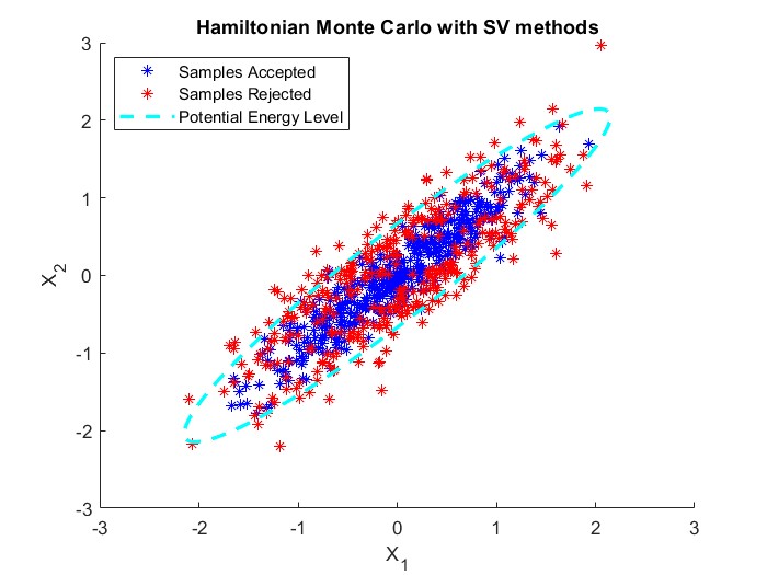
(a) AR=0.6610

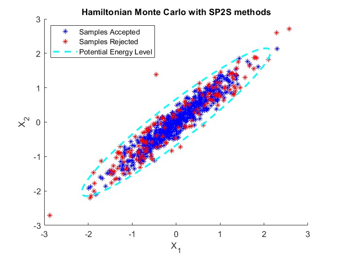
(b) AR=0.842

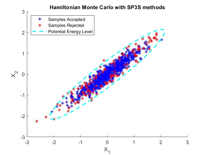
(c) AR=0.882

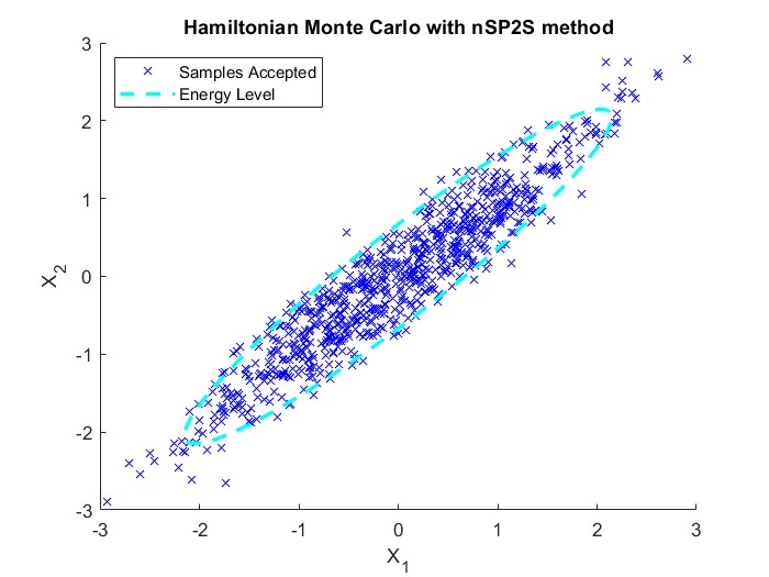
(d) AR=1

Figure 1: Accepted and rejected samples of different integrator, for a Bivariate distribution. Iterations of HMC samples with $T^{*}=5$ and $h=0.005$ for (a), (b), (c), and $h\,=h_{b_{max}}\,\approx 1.3432$ for (d).

6.2 Multivariate Gaussian distribution

Regarding a more general case, we have considered, as a target a multivariate Gaussian distribution as considered in [23] in the same form adopted in [5] i.e.

$$\pi(\mathbf{q})\propto\Bigg{(}-\frac{1}{2}\sum_{j=1}^{d}j^{2}q^{2}_{j}\Bigg{)}.$$

We consider different dimensions, from $d=256$ to $d=1024$ with potential energy function $U(\mathbf{Q})=\dfrac{1}{2}\,\mathbf{Q}^{T}\,D_{\alpha}^{-1}\,\mathbf{Q}$ in which the variables are independent, with zero mean and $D_{\alpha}$ entries given by standard deviations $\alpha_{j}\,={1/j^{2}}$ for $j=1,\dots,d$. Kinetic energy function $K(\mathbf{P})\,=\,\dfrac{1}{2}\,\mathbf{P}^{T}\,\mathbf{P}$ is set as above.

For the experiments we compared our algorithm (23) applied with $\Sigma=D_{\alpha}^{-1/2}$ with the family of integrators considered in [7]. This kind of integrators are second order accurate and depend on a real parameter. The authors consider different integrators by varying the value of the parameter (see [7] for the details of integrators). For our purpose we chose as competitors, only those that in the paper are called LF, and BlCaSa. The first because it corresponds to three consecutive time-steps of the classic Störmer-Verlet (or equivalently, LeapFrog) method (15), the second because it is the most performing one when considering the case of multivariate Gaussian [7]. We do not consider here further improvements of the methods as provided in [6], as, likewise the previous methods, they do not retain the energy of Gaussian distributions.

To perform the experiments we used the same parameters used in the paper [7].

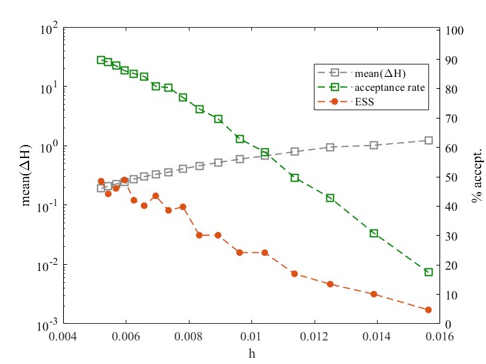
(a) LF

(b) BlCaSa

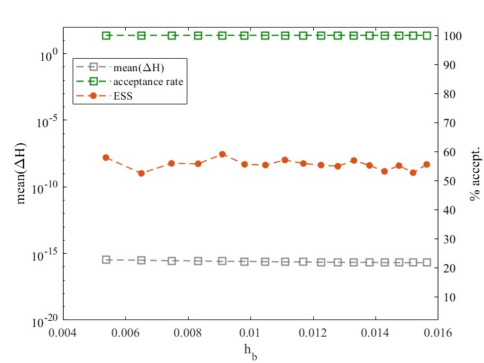
(c) nSP2S-1

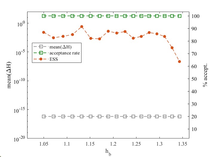
(d) nSP2S-2

Figure 2: Multivariate Gaussian target with d=256; acceptance rate percentage (green squares), mean of $\Delta H$ (grey squares) and ESS percentage (orange points) comparison for $LF$, $BlCaSa$ integrators, measuring with different step size $h$ and nSP$2$S-1 and nSP$2$S-2 by varying $h_{b}$.

In particular, the number of samples, each of dimension $d=256$, has been set to $L=5000$ choosing a number of burn-in samples equal to $1000$. The initial $\mathbf{q}^{(1)}$ is drawn from the target $\pi(\mathbf{q})$. For LF and for BlCaSa we choose path length $T^{*}=5$ and the time-steps $N=320,360,\ldots,960$, with a corresponding step sizes $h=5/320,5/360,\ldots,5/960$ ($h$ then varies between $\approx 1.6\times 10^{-2}$ and $5.2\times 10^{-3}$). For our method, where the step size $h_{b}$ depends from the parameter $b$, we performed two different experiments. The first, called nSP$2$S-$1$ aims at making a fair comparison with LF and for BlCaSa: we choose different values of parameter b in the range $(0.1909831513,0.1909842368)$ which make the corresponding step sizes $h_{b}$, time-steps $N$ and path length $T^{*}=5$ equal to those used by competitors. In the second experiment, called nSP$2$S-$2$, we show the performance of the proposed integrator for values of the parameter $b$ in the range $(0.1968,0.2008)$ that provide large step sizes $h_{b}$ varying between $1.05$ and $1.35$. In this case the time-interval has been randomized with $\pm 40\%$ variations around $5$, with this ensuring that $3<T^{*}<7$. For all the experiment we have measured the acceptance rate, the mean of $4000$ samples of the energy errors $\Delta H^{(i)}(\mathbf{q}^{(i)},\mathbf{p}^{(i)})=H(\mathbf{q}^{*},\mathbf{p}^{*})-H(\mathbf{q}^{(i)},\mathbf{p}^{(i)})$ and the effective sample size ESS of the first component $q_{1}^{(i)}$ of $\mathbf{q}^{(i)}$ which corresponds to the component with largest standard deviation $\alpha_{1}=1$ (see [18]).

In Figure 2 on the left vertical axis, the means of the energy errors (gray square), are reported on a logarithmic scale, for the different values of the stepsize $h$. On the right vertical axis, for the LF (a), for BlCaSa(b) and for the first experiment with nSP$2$S method (c), the accepted percentage rate (green square) and the ESS (orange circle) are plotted in linear scale. In (d) the same quantities versus step size $h_{b}$ are depicted for the second experiment performed with the nSP$2$S method. As expected in both cases (c) and (d), our approach has a $100\%$ acceptance rate with mean of energy errors of order $10^{-16}$. In particular the ESS remains above $60\%$ in both cases. It’s worth noting that the computational cost of the experiment nSP$2$S-$2$ is much lower than the experiment nSP$2$S-$1$ as a larger step size has been adopted without decrement in terms of performance.

In addition, for a reduced number of samples $L=1000$, we performed a qualitative comparative analysis among the methods by estimating the mean and the standard deviation of the samples.

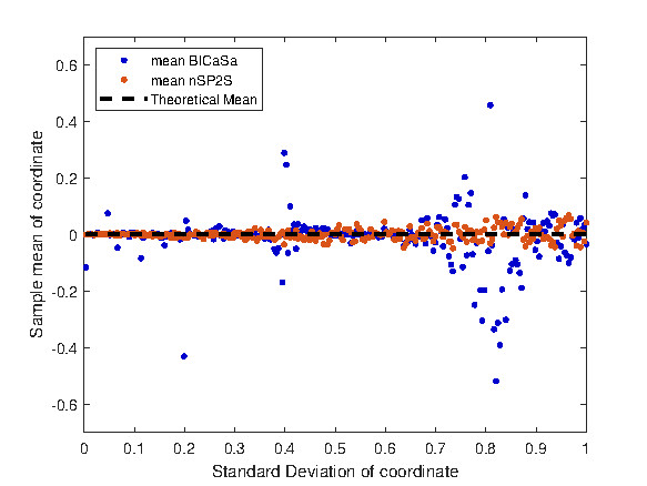
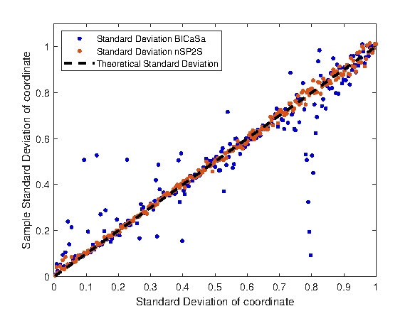
Figure 3: Multivariate distribution. Estimates of means (left) and standard deviations (right) for the $d=256$ dimensional example. On the $x$-axes are reported the standard deviations $\alpha_{j}$ of each variable $q_{j}$ for $j=\,1,\dots,d$, on the $y$-axes the estimated values each evaluated from $L=1000$ iterations, are reported.

We run BlCaSa by setting $h=0.014$ and $N=5/h$ and nSP$2$S with $b=0.191$, $h_{b}=0.0580$ and $N=25$. The estimates for the mean and the standard deviations, evaluated as simple means and standard deviations of the values from the $L\,=1000$ iterations for each of the $d\,=256$ variables, against the theoretical values of standard deviations $\alpha_{j}$, for $j=1,\dots,\,d$, are shown in Figure 3. Notice that the error in the estimates for the means and standard deviations obtained with the HMC algorithm with trajectories evaluated with nSP$2$S appears even better than the ones provided by HCM with BlCaSa method. Of course, the saving in computational cost was very evident as, for each iteration, only $N=25$ steps of nSP$2$S method are necessary and all proposals accepted, despite the $N=357$ steps used by the BlCaSa method with $128$ proposals rejected. Finally, in Figure 4 we compare the integrators in terms of ESS per unit computational work i.e. ESS$\times h$ for the different values of the step size $h$. As can be seen, BlCaSa results very efficient also with value of $h$ greater then $8\times 10^{-3}$; however nSP$2$S turns out to be the best method because its maximum value is the highest among the maximum values reached by the other two methods.

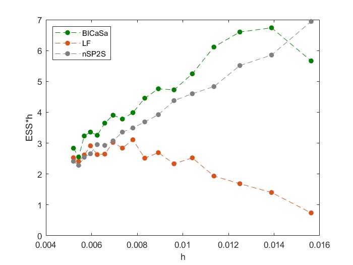
Figure 4: Comparison of the integrators computational cost ESS per time-step/per unit for sampling from Multivariate Gaussian target with $d=256$ by varyng step size $h$. LF (orange points), BlCaSa (green points) and nSP2S (grey points).

6.3 Perturbed Gaussian models

In this class we consider models where, after a suitable change of variables if needed, the potential energy function can be expressed as

(24) $$U(\mathbf{Q})\,=\,\dfrac{1}{2}\mathbf{Q}^{T}\,\,\mathbf{Q}+\epsilon\,f(\mathbf{Q}),\quad 0<\epsilon\leq 1.$$

We associate a kinetic energy function $K(\mathbf{P})\,=\,\dfrac{1}{2}\,\mathbf{P}^{T}\,\mathbf{P}$ so that the Hamiltonian can be written as

(25) $$K(\mathbf{P})\,+\,U(\mathbf{Q})\,=\,\dfrac{1}{2}\mathbf{P}^{T}\,\mathbf{P}\,+\,\dfrac{1}{2}\,\mathbf{Q}^{T}\mathbf{Q}\,+\,\epsilon\,f(\mathbf{Q})$$

and the Hamiltonian system is given by

(26) $$\dfrac{d\mathbf{Q}}{dt}\,=\,\mathbf{P},\qquad\dfrac{d\mathbf{P}}{dt}\,=\,-\mathbf{Q}\displaystyle-\epsilon\,\nabla_{\mathbf{Q}}\,f(\mathbf{Q})$$

We apply the method (16) within the Algorithm 3 which provides an energy preserving method for the above Hamiltonian system when $\epsilon=0$. We investigate the performance of the algorithm with respect to the acceptance rates and to the error in energy at $\epsilon=1$ for two different specific models: the logistic regression and the Log-Gaussian Cox model.

6.4 Log-Gaussian Cox model

As first example we considered, as target, the Log-Gaussian Cox distribution [21]. For this model the data set is organized in the vector $\mathbf{X}\,=\left[X_{1,1},\dots,X_{1,d},X_{2,1},\dots,X_{2,d},\dots X_{d,1},\dots X_{d,d}\right]^{T}$, representing the number of points $X_{i,j}$ in each cell $(i,j)$ of a $d\times d$ dimensional grid in $[0,1]\times[0,1]$. The purpose is to sample the variable $\mathbf{Y}=\left[Y_{1,1},\dots,Y_{1,d},Y_{2,1},\dots,Y_{2,d},\dots Y_{d,1},\dots Y_{d,d}\right]^{T}$ from the probability distribution given by

$$\mathcal{P}(\mathbf{Y})=\prod_{i,j=1}^{d}\exp(X_{i,j}Y_{i,j}-m\exp(Y_{i,j})\,)\,\exp\left(-\dfrac{1}{2}(\mathbf{Y}-\mu\mathbf{1})^{T}\,S^{-1}(\mathbf{Y}-\mu\mathbf{1})\right)$$

where $m=1/d^{2}$ represents the area of each cell and the matrix $S$ is given

$$S=\left(\begin{array}[]{cccccc}T_{1}&T_{2}&T_{3}&\dots&\dots&T_{d}\\ T_{2}&T_{1}&T_{2}&\ldots&&\vdots\\ T_{3}&T_{2}&\ldots&\ldots&\ldots&\ldots\\ \vdots&\ldots&\ldots&\ldots&T_{2}&T_{3}\\ \vdots&&\ldots&T_{2}&T_{1}&T_{2}\\ T_{d}&\dots&\dots&T_{3}&T_{2}&T_{1}\end{array}\right),\,\,\,T_{i}(k,j)=\sigma^{2}\,e^{-\frac{\sqrt{(1-i)^{2}+(k-j)^{2}}}{\beta\,d}},\,\,\,i,\,k,\,j=1,\dots d.$$

with $\sigma^{2}$, $\beta$, are fixed parameters and $\mu=\log\left(\displaystyle\sum_{i,j=1}^{d}X_{i,j}\right)-\sigma^{2}/2$. The potential energy function is defined as

$$\small\begin{array}[]{ccc}U(\mathbf{Y})\,=\,-\log\left[\mathcal{P}(\mathbf{Y})\right]&=&\displaystyle\sum_{i,j=1}^{d}m\exp(Y_{i,j})-X_{i,j}Y_{i,j}\,+\,\dfrac{1}{2}(\mathbf{Y}-\mu\mathbf{1})^{T}\,S^{-1}(\mathbf{Y}-\mu\mathbf{1})\\ &=&\dfrac{1}{2}(\mathbf{Y}-\mu\mathbf{1})^{T}\,S^{-1}(\mathbf{Y}-\mu\mathbf{1})\,+\,\displaystyle m\,\mathbf{1}^{T}\exp(\mathbf{Y})-\mathbf{X}^{T}\mathbf{Y}.\end{array}$$

For the application of the proposed procedure, we take $L$ as the factor of the Cholesky factorization of $S^{-1}$ so that $S^{-1}\,=\,L^{T}\,L$. In terms of the novel variable $\mathbf{Q}:=L\,(\mathbf{Y}-\mu\mathbf{1})$, the potential energy function can be expressed as in (24) with ($\epsilon=1$)

$$f(\mathbf{Q}):=\displaystyle m\,\mathbf{1}^{T}\exp(L^{-1}\mathbf{Q}+\mu\mathbf{1})-\mathbf{X}^{T}\left(L^{-1}\mathbf{Q}+\mu\mathbf{1}\right).$$

When we associate a kinetic energy function $K(\mathbf{P})\,=\,\dfrac{1}{2}\,\mathbf{P}^{T}\,\mathbf{P}$, the Hamiltonian can be written as in (25) and the Hamiltonian system is given by (26) with

$$\nabla_{\mathbf{Q}}\,f(\mathbf{Q})\,=\,m\,{L^{-T}}\exp({L}^{-1}\mathbf{Q}+\mu\mathbf{1})-{L^{-T}}\,\mathbf{X}.$$

The sampling values of the original variable are obtained by exploiting the relation $\mathbf{Y}={L}^{-1}\mathbf{Q}+\mu\mathbf{1}$.

The Log-Gaussian Cox model is particularly relevant as point process to model presence-only species distribution [27], as the case of Scots pines in the Eastern Finland [21, 9] or the spread of the invasive species Eucalyptus sparsifolia, in Australia [27]. In our study, we approach a similar problem of alien plants as the highly competitive woody invasive species Ailanthus altissima (Mill.) Swingle, thriving in Murgia Alta Natura 2000 protected area and National Park (southern Italy). Ailanthus altissima, also known as tree-of-heaven, is an invasive deciduous plant of Asian origin recognized as one of the most widespread and harmful invasive plants in both USA [22] and Europe (www.europe-aliens.org) which are causing impoverishment in natural habitats as one of the most important causes of local and regional biodiversity loss, ecosystem degradation, diminishing both abundance and survival of native species [8]. In our tests, we considered as data set the mapping at very high spatial resolution ($2$ m) of the Ailanthus altissima presence obtained by considering multi-temporal remote sensing satellite data and machine learning techniques, based on a two-stage hybrid classification process [29].

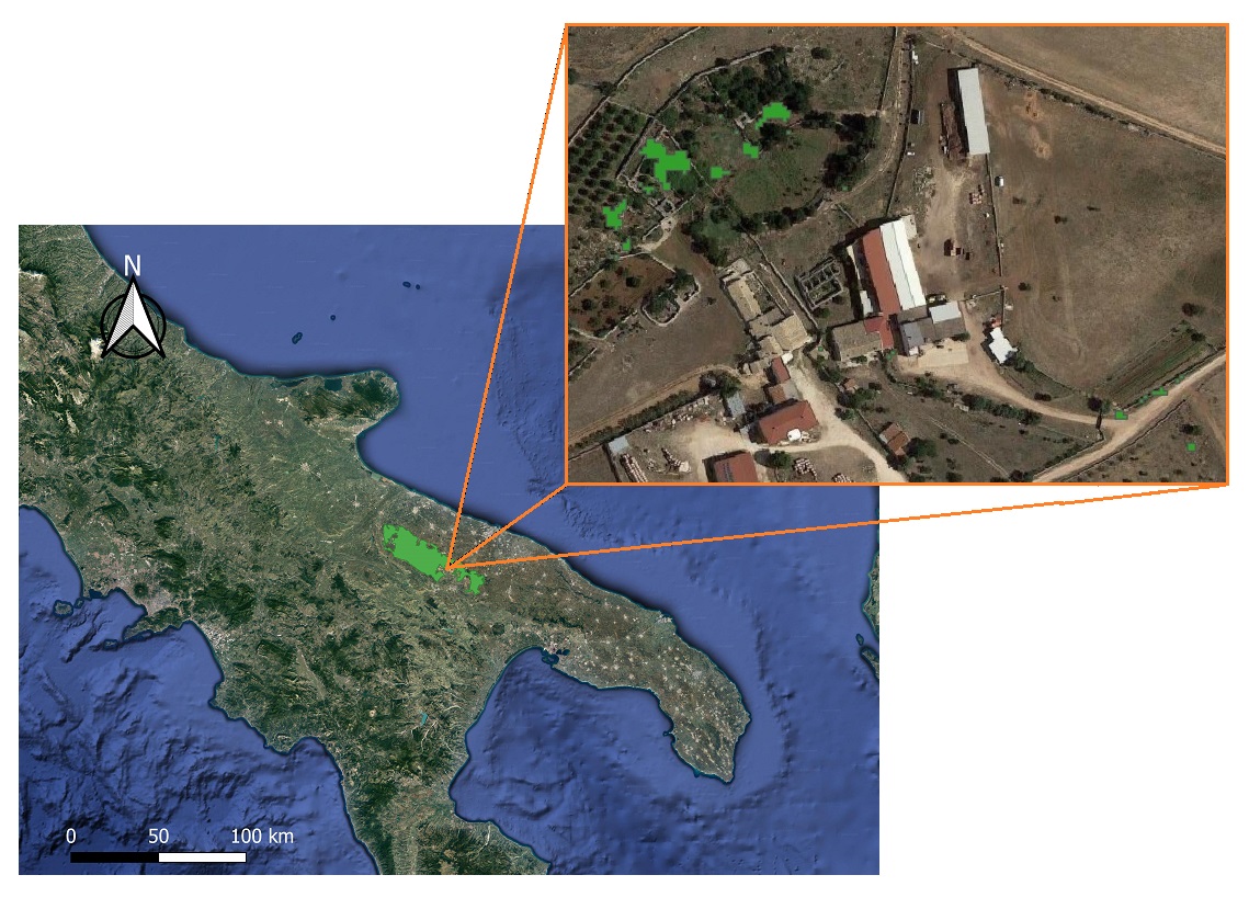
Figure 5: Detail with zoom of the area taken into consideration in Alta Murgia Natura 2000 protected area and National Park (southern Italy)

The images considered for the dataset were provided by the European Space Agency (ESA) under the Data Warehouse 2011-2014 policy within the FP7-SPACE BIO_SOS project www.biosos.eu and European LIFE project (LIFE12 218 BIO/IT/000213). In particular, from the entire dataset we extracted a small area containing $185$ trees as shown in Figure 5. After scaling the data between $0$ and $1$ we used a grid size $d=64$ and we calculated the parameters of the Log Gaussian Cox model by using the methodology of Moment-based estimation described in [10]. The resulting parameters are $\beta=0.127$, $\sigma^{2}=3.5881$ and $\mu=\log(185)-\sigma^{2}/2$. We set the path length $T=3$ and the step size $h$ and $h_{b}$ in the interval $[0.3,\,0.05]$ with corresponding $N$ ranging from $60$ to $10$. We collect L=5000 Markov chain after 1000 burn-in samples. In Figure 6, we have reported the results in terms of acceptance percentage and mean of the energy errors. The horizontal axis of each plot indicates the step size $h$, and $h_{b}$, for the competitors methods and for our method, respectively. We clearly see how our method outperforms the competitors, reaching acceptance rates greater than $90\%$ with all $h_{b}$ values and with an average energy error which always remains very low. Finally in the Figure 7, we show the results obtained through the application of the Algorithm 3. Starting from $b_{init}=b_{BCS}=0.2113$ (case $2$ of Section 5.1) and a reduction factor of $red\sim 10^{-4}$, after a few steps the method allows to achieve the best configuration for $b$ and $h_{b}$ yielding the maximum acceptance rate. In the right part of the figure we show the estimate of the intensity map of the Ailanthus trees obtained with the values of $b$ and $h_{b}$ previously estimated.

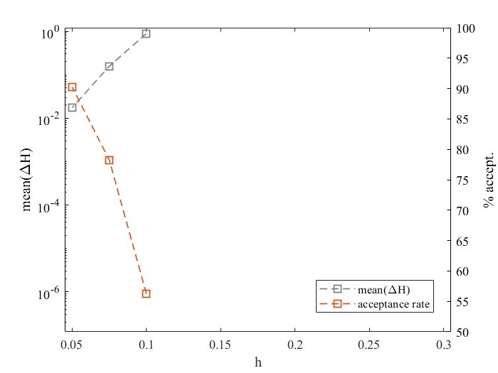
(a) LF

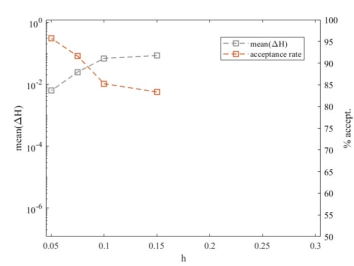
(b) BlCaSa

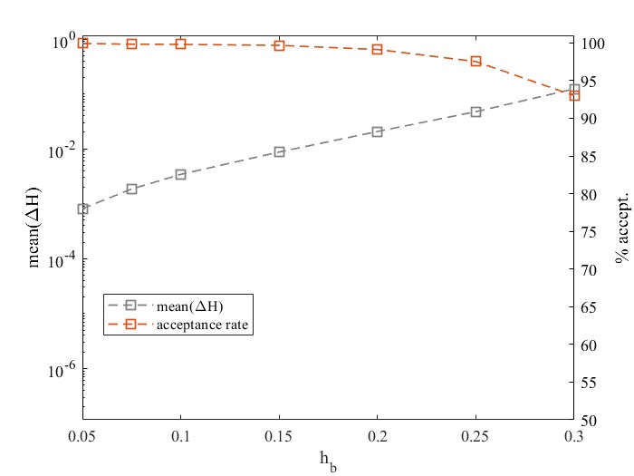
(c) nSP2S

Figure 6: Log-Gaussian Cox target. Acceptance rate (orange sqares), mean of $\Delta H$ (grey sqares) against different step size $h$ for LF (a), BlCaSa (b) and $h_{b}$ for nSP2S (c).

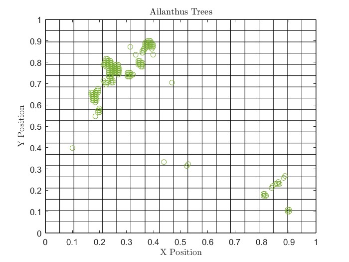
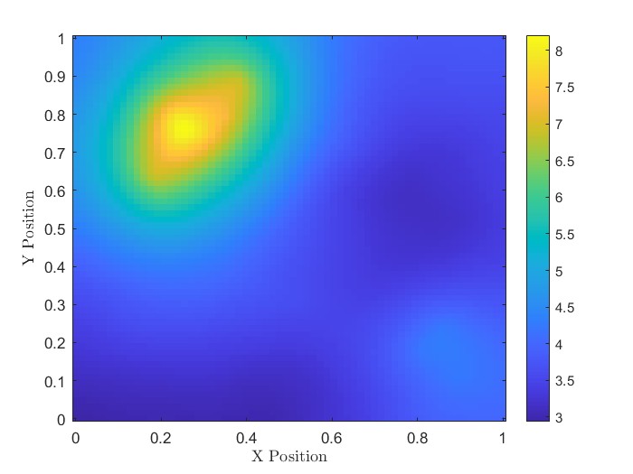
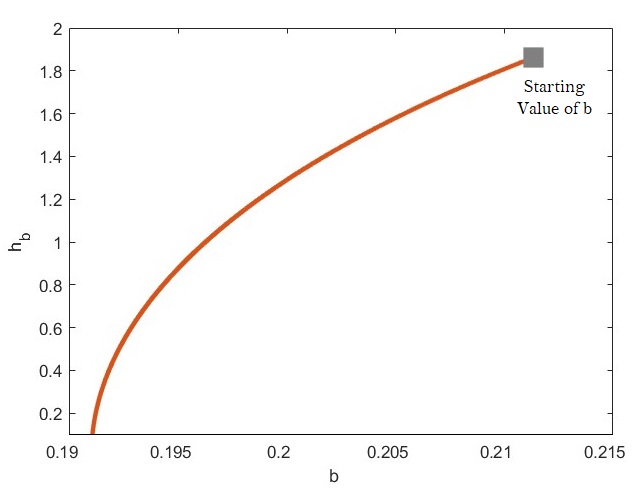
Figure 7: Presence of Ailanthus trees (up, on the left), position of the trees (green points) suitably scaled between $0$ and $1$. Estimated intensity map of Ailhantus obtained with the final choice of $b$ and $h_{b}$ accordingly to the Algorithm 3 (up, on the right). Adaptive choice of $b$ against $h_{b}$ (down)

6.5 Logistic regression model

As second example of perturbed Gaussian model distributions we have considered a Bayesian Logistic regression model. By adopting the same notations in [30], we indicate with $\mathbf{Y}=[Y_{1},\ldots Y_{n}]^{T}$ the $n$-dimensional vector of the labels associated to the instances matrix $X\in\mathbb{R}^{n\times(d+1)}.$ Let $\mathbf{x}_{k}=[X_{k,0},\ldots,X_{k,d}]^{T}$ the $(d+1)$-dimensional (column) vector corresponding to the $k$th row of the matrix $X$, for $k=1,\ldots,n.$ The regression coefficients for the $d$ covariates and the intercept are collected in the vector $\bm{\beta}=[\beta_{0},\beta_{1},\ldots,\beta_{d}]^{T}$. We specify a multivariate normal prior for $\bm{\beta}$ with covariance matrix $D=\sigma^{2}I$, where $I$ is the $(d+1)$-dimensional identity matrix and $\sigma^{2}$ is the variance, freely chosen. The purpose is to sample the parameters $\bm{\beta}$ that follow the distribution:

$$\small\begin{array}[]{rcl}\mathcal{P}(\bm{\beta})&\propto&\exp\Big{(}\bm{\beta}^{T}X^{T}\left(\mathbf{Y-\mathbf{1}_{n}}\right)-\displaystyle\sum_{j=1}^{n}\Big{[}\log(1+\exp(-\mathbf{x}_{j}^{T}\bm{\beta})\Big{]}\Big{)}\,\exp\Big{(}-\frac{1}{2}\bm{\beta}^{T}D^{-1}\bm{\beta}\Big{)}\\ \\ &=&\exp\Big{(}\bm{\beta}^{T}X^{T}\mathbf{Y}-\displaystyle\sum_{j=1}^{n}\Big{[}\log(1+\exp(\mathbf{x}_{j}^{T}\bm{\beta})\Big{]}\Big{)}\,\exp\Big{(}-\frac{1}{2}\bm{\beta}^{T}D^{-1}\bm{\beta}\Big{)}\end{array}$$

The potential energy function, in term of the variable $\mathbf{Q}=\bm{\beta}/\sigma$ is defined as:

$$U(\mathbf{Q})=-\log[\mathcal{P}(\mathbf{Q})]\,=\,\frac{1}{2}\,\mathbf{Q}^{T}\mathbf{Q}+\sum_{k=1}^{n}\Big{[}\log(1+\exp(\sigma\,\mathbf{x}_{k}^{T}\mathbf{Q}))\Big{]}-\sigma\,\mathbf{Q}^{T}{X}^{T}\mathbf{Y}$$

Without loosing of generality, we can set $\sigma=1$ as the same results are obtained on the scaled dataset $\tilde{X}=X/\sigma$. Consequently, it can be expressed as in (24) ($\epsilon=1$) with

$$f(\mathbf{Q}):=\displaystyle\sum_{k=1}^{n}\Big{[}\log(1+\exp(\mathbf{x}_{k}^{T}\mathbf{Q}))\Big{]}-\,\mathbf{Q}^{T}{X}^{T}\mathbf{Y}.$$

We associate a kinetic energy function $K(\mathbf{P})\,=\,\dfrac{1}{2}\,\mathbf{P}^{T}\,\mathbf{P}$ so that the Hamiltonian can be written as in (25) and the Hamiltonian system is given by (26) with

$$\nabla_{\mathbf{Q}}\,f(\mathbf{Q})=-\,X^{T}\bigg{(}\mathbf{Y}-\bigg{[}\frac{\exp(\,\mathbf{x}_{1}^{T}\mathbf{Q})}{1+\exp(\mathbf{x}_{1}^{T}\mathbf{Q})},\frac{\exp(\mathbf{x}_{2}^{T}\mathbf{Q})}{1+\exp(\mathbf{x}_{2}^{T}\mathbf{Q})},\dots,\frac{\exp(\mathbf{x}_{n}^{T}\mathbf{Q})}{1+\exp(\mathbf{x}_{n}^{T}\mathbf{Q})}\bigg{]}^{T}\bigg{)}.$$

As $\sigma=1$, the sampling values of the original variable are given by $\bm{\beta}=\sigma\,\mathbf{Q}=\mathbf{Q}$. For this experiment we used the benchmark classification dataset from the UCI repository [2], that consists in different matrices of instances and labels. Here we show the results obtained with the Pima Indian dataset, although we also tested the other datasets, Ripley, Heart, German credit, and Australian credit, obtaining results in line with those shown here.

As is commonly used, we normalize the dataset with $0$ mean and standard deviation $1$ after a scaling procedure of data according to the choosing value of $\sigma$.

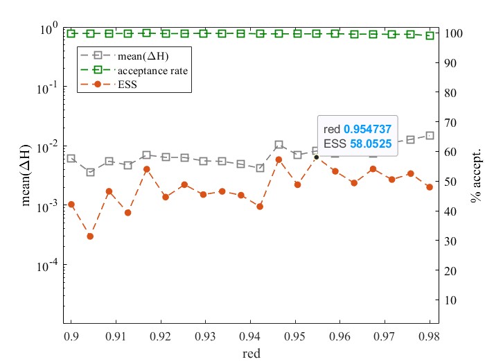
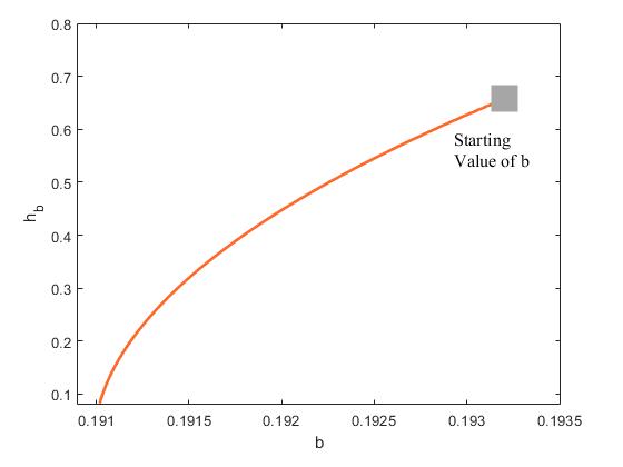
Figure 8: Logistic Regression target; acceptance rate percentage (green squares), mean of $\Delta H$ (grey squares) and ESS percentage (orange points) measuring with different values of $red$ in the Algorithm 3 (a). Adaptive choice of b against $h_{b}$ (b).

We test the performance of the proposed integrator built on the proposed adaptive approach 3 by setting, the path length $T=3$, $b_{max}=0.1932$ (case $4$ of Section 5.1). In all the experiment we collect $L=5000$ Markov chain after 1000 burn-in samples and for each iteration we randomize the time-step $N=T/h_{b}$ by allowing $\pm 10\%$ to avoid a low number of ESS [23].

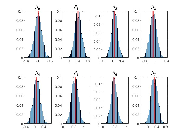
Figure 9: Logistic Regression with Pima Indian dataset. Analisys of posterior estimates HMC-nSP2S (histograms) and frequentist estimates (vertical lines) with glm

For this experiment we perform the tests by varying the reduction parameter $red$ within the range $(0.9,0.98)$ and measuring for each of these values the efficiency in term of acceptance percentage, mean of energy errors end ESS calculated as the mean of the ESS on each regression coefficients $\mathbf{q}^{(i)}=[\beta_{0}^{(i)},\beta_{1}^{(i)},\ldots\beta_{d}^{(i)}]$ with $i=1000,\ldots,5000$. The results obtained are shown in Figure 8 (a). For each values of $red$ the adaptive algorithm reaches an high percentage of AR. In particular $red=0.954737$ represents the best values that ensures a high acceptance rate along with a high percentage of ESS. Given this reduction value, the Figure 8 (b) shows how $b$ changes with respect to $h_{b}$ reaching, automatically, the best configuration for the sampler. Moreover the estimated samples $\bm{\beta}$ are deemed to be in accordance with frequency estimates calculated with the generalized linear model (glm) [24]. This is clearly shown in Figure 9 where the frequentist estimates (red line) falls in the central location of the histograms of $\beta_{0},\beta_{1},\ldots,\beta_{7}$.

7 Conclusions

The very recent research literature on searching for efficient volume-preserving and reversible integrators able to replace the Störmer Verlet in the practical implementation of the HMC method, uses as yardstick the ability of the numerical algorithms to reduce the expectation of the energy error variable when applied to univariate and multivariariate Gaussian distributions [7],[5]. However, none of the above studies makes an explicit reference to the possibility of properly selecting the parameters in order to exactly preserve the Hamiltonian in order to have zero as expectation value of the energy error.

In this paper, we analyzed a representation of linear maps corresponding to trajectories evaluated by mean of symplectic reversible splitting schemes for sampling from Gaussian distributions. In our formulation (different from the one proposed in [5]), the expression of the expectation value of the energy error gives evidence of the role of the quantity which is solely responsible for the distortion in calculated energy. Minimizing this quantity results in reducing the number of rejections in practical implementation of the HMC algorithm; consequently, methods with this quantity equal to zero are optimal for Gaussian univariate and multivariate distributions in terms of accepted proposals.

Within the one-parameter family of second order splitting methods considered in this paper, we show that a properly selection of the step size allows to retain the energy for univariate and multivariate Gaussian distributions. As all proposals are accepted by construction, the proposed method outperforms the numerical competitors given in [7, 6] which are neither optimal for Gaussian distributions (as they are not energy-preserving methods) nor less expensive than the ones considered here.

For more general distributions, which can be interpreted as perturbed Gaussian distributions, the same criterion for the selection of the step size is proposed. The resulting nice performances are also enhanced by the application of an adaptive selection of the parameter $b$ which detects one method in the family of the one-parameter splitting integrators. Specifically, starting from a suitable large initial value for $b$, we reduce its value of a given percentage each time a sample is not accepted.

In order to validate the effectiveness of the new approach we tested the algorithm also for general classes of target distribution as the the Log-Gaussian Cox model and the Bayesian logistic regression, in particular the first one is relevant as point process to model presence-only species distribution of invasive species [27]. In our test, we considered as data set the mapping at very high spatial resolution of the Ailanthus altissima presence in Alta Murgia National Park [29].

Our promising preliminar results require to exploit the use of more robust criteria for an adaptive method’s selection in one-parameter families of integrators having the objective of reducing the number of rejections. This can be the subject of a future research direction.

References

- [1] Berni J Alder and Thomas Everett Wainwright “Studies in molecular dynamics. I. General method” In The Journal of Chemical Physics 31.2 American Institute of Physics, 1959, pp. 459–466
- [2] Kevin Bache and Moshe Lichman “UCI machine learning repository” Irvine, CA, USA, 2013
- [3] Christopher M Baker et al. “Optimal control of invasive species through a dynamical systems approach” In Nonlinear Analysis: Real World Applications 49 Elsevier, 2019, pp. 45–70
- [4] Christopher M Baker et al. “Optimal spatiotemporal effort allocation for invasive species removal incorporating a removal handling time and budget” In Natural Resource Modeling 31.4 Wiley Online Library, 2018, pp. e12190
- [5] Sergio Blanes, Fernando Casas and JM Sanz-Serna “Numerical integrators for the Hybrid Monte Carlo method” In SIAM Journal on Scientific Computing 36.4 SIAM, 2014, pp. A1556–A1580
- [6] Sergio Blanes, Mari Paz Calvo, Fernando Casas and Jesús Marı́a Sanz-Serna “Symmetrically processed splitting integrators for enhanced Hamiltonian Monte Carlo sampling” In SIAM Journal on Scientific Computing 43.5 SIAM, 2021, pp. A3357–A3371
- [7] Mari Paz Calvo, Daniel Sanz-Alonso and JM Sanz-Serna “HMC: avoiding rejections by not using leapfrog and some results on the acceptance rate” In arXiv preprint arXiv:1912.03253, 2019
- [8] Francesca Casella, Michele Vurro and A.G. Boari “Restoration of areas infested by A. altissima in the Alta Murgia National Park: experience within a LIFE project.” In Seventh International Weed Science Congress, 2016, pp. 215 Prague, Czech Republic
- [9] Ole Christensen, Gareth Roberts and Jeffrey Rosenthal “Scaling Limits for the Transient Phase of Local Metropolis-Hastings Algorithms” In Journal of the Royal Statistical Society Series B 67, 2003 DOI: 10.1111/j.1467-9868.2005.00500.x
- [10] Peter Diggle, Paula Moraga, Barry Rowlingson and Benjamin Taylor “Spatial and Spatio-Temporal Log-Gaussian Cox Processes: Extending the Geostatistical Paradigm” In Statistical Science 28, 2013 DOI: 10.1214/13-STS441
- [11] Simon Duane, Anthony D Kennedy, Brian J Pendleton and Duncan Roweth “Hybrid monte carlo” In Physics letters B 195.2 Elsevier, 1987, pp. 216–222
- [12] Ernst Hairer, Christian Lubich and Gerhard Wanner “Geometric numerical integration illustrated by the Stormer-Verlet method” In Acta numerica 12.12, 2003, pp. 399–450
- [13] Balint Joo et al. “Instability in the molecular dynamics step of a hybrid Monte Carlo algorithm in dynamical fermion lattice QCD simulations” In Physical Review D 62.11 APS, 2000, pp. 114501
- [14] Deborah Lacitignola, Fasma Diele and Carmela Marangi “Dynamical scenarios from a two-patch predator–prey system with human control–Implications for the conservation of the wolf in the Alta Murgia National Park” In Ecological modelling 316 Elsevier, 2015, pp. 28–40
- [15] Benedict Leimkuhler and Charles Matthews “Robust and efficient configurational molecular sampling via Langevin dynamics” In The Journal of chemical physics 138.17 American Institute of Physics, 2013, pp. 05B601_1
- [16] Benedict Leimkuhler and Sebastian Reich “Simulating hamiltonian dynamics” Cambridge university press, 2004
- [17] Carmela Marangi et al. “Mathematical tools for controlling invasive species in Protected Areas” In Mathematical Approach to Climate Change and its Impacts Springer, 2020, pp. 211–237
- [18] Luca Martino, Víctor Elvira and Francisco Louzada “Effective sample size for importance sampling based on discrepancy measures” In Signal Processing 131, 2017, pp. 386–401 DOI: https://doi.org/10.1016/j.sigpro.2016.08.025
- [19] Robert I McLachlan “On the numerical integration of ordinary differential equations by symmetric composition methods” In SIAM Journal on Scientific Computing 16.1 SIAM, 1995, pp. 151–168
- [20] Nicholas Metropolis et al. “Equation of state calculations by fast computing machines” In The journal of chemical physics 21.6 American Institute of Physics, 1953, pp. 1087–1092
- [21] Jesper Møller, Anne Randi Syversveen and Rasmus Plenge Waagepetersen “Log gaussian cox processes” In Scandinavian journal of statistics 25.3 Wiley Online Library, 1998, pp. 451–482
- [22] Harini Nagendra et al. “Remote sensing for conservation monitoring: assessing protected areas, habitat extent, habitat condition, species diversity and threats.” In Ecological Indicators 33, 2013, pp. 45–59 DOI: 10.1016/j.ecolind.2012.09.014
- [23] Radford M Neal “MCMC using Hamiltonian dynamics” In Handbook of markov chain monte carlo 2.11, 2011, pp. 2
- [24] J.. Nelder and R… Wedderburn “Generalized Linear Models” In Journal of the Royal Statistical Society. Series A (General) 135.3 [Royal Statistical Society, Wiley], 1972, pp. 370–384 URL: http://www.jstor.org/stable/2344614
- [25] Brigida Pace, Fasma Diele and Carmela Marangi “Splitting schemes and energy preservation for separable Hamiltonian systems” In Mathematics and Computers in Simulation 110 Elsevier, 2015, pp. 40–52
- [26] Cristian Predescu et al. “Computationally efficient molecular dynamics integrators with improved sampling accuracy” In Molecular Physics 110.9-10 Taylor & Francis, 2012, pp. 967–983
- [27] Ian W. Renner et al. “Point process models for presence-only analysis” In Methods in Ecology and Evolution 6, 2015, pp. 366–379 DOI: 10.1111/2041-210X.12352
- [28] Tetsuya Takaishi and Philippe De Forcrand “Testing and tuning symplectic integrators for the hybrid Monte Carlo algorithm in lattice QCD” In Physical Review E 73.3 APS, 2006, pp. 036706
- [29] Cristina Tarantino et al. “Ailanthus altissima mapping from multi-temporal very high resolution satellite images” In ISPRS Journal of Photogrammetry and Remote Sensing 147, 2019, pp. 90–103 DOI: 10.1016/j.isprsjprs.2018.11.013
- [30] Samuel Thomas and Wanzhu Tu “Learning Hamiltonian Monte Carlo in R” In The American Statistician 75.4 Taylor & Francis, 2021, pp. 403–413