Abstract

The statistical significance that characterizes a discrepancy between a measurement and theoretical prediction is usually calculated assuming that the statistical and systematic uncertainties are known. Many types of systematic uncertainties are, however, estimated on the basis of approximate procedures and thus the values of the assigned errors are themselves uncertain. Here the impact of the uncertainty on the assigned uncertainty is investigated in the context of the muon $g-2$ anomaly. The significance of the observed discrepancy between the Standard Model prediction of the muon’s anomalous magnetic moment and measured values are shown to decrease substantially if the relative uncertainty in the uncertainty assigned to the Standard Model prediction exceeds around 30%. The reduction in sensitivity increases for higher significance, so that establishing a $5\sigma$ effect will require not only small uncertainties but the uncertainties themselves must be estimated accurately to correspond to one standard deviation.

Keywords: systematic uncertainties, statistical significance, muon $g-2$, gamma variance model, Bartlett correction

1 Introduction

The recent measurement of the muon’s anomalous magnetic moment at Fermilab’s Muon $g-2$ Experiment [1], when averaged with the 2006 value from Brookhaven [2] was found to be in disagreement with the Standard Model (SM) prediction [3] with a significance of $4.2\sigma$.

The significance of the discrepancy treats both the measurements and the theoretical prediction as Gaussian distributed quantities whose standard deviations are exactly known. Although the statistical errors are no doubt estimated with negligible uncertainty, this is not necessarily the case for systematic errors, particularly those of the SM prediction.

Here the method for incorporating uncertainties on reported systematic errors of Ref. [4] is applied to the muon $g-2$ significance. Section 2 describes the input values for the analysis and Sec. 3 gives a brief description of the statistical model. Results are shown in Sec. 4 and finally some conclusions are drawn in Sec. 5.

The recent result from Borsanyi et al. [5] using lattice QCD gives an SM prediction for $g-2$ that differs less from the measured value. As the purpose of this note is to illustrate the importance of the assigned systematic uncertainty for the case of a significant discrepancy, we focus on the $4.2\sigma$ difference highlighted in Ref. [1] and leave the lattice result for future consideration.

2 Input values

To simplify the numerical treatment and presentation of the results, the values $a_{\mu}=(g-2)/2$ are transformed according to

$$y=a_{\mu}\times 10^{9}-1165900\;.$$ (1)

The recent FNAL measurement [1] when combined with the 2006 value from BNL [2] results in an averaged experimental value of

$$y_{\rm exp}=20.61\pm 0.41\;.$$

The uncertainty reflects both statistical (0.37) and systematic (0.17) errors. The Standard Model prediction is given in Ref. [3] as

$$y_{\rm SM}=18.10\pm 0.43\;.$$

The uncertainty is dominated by the hadronic vacuum polarization (0.40) and to a lesser extent the hadronic light-by-light contribution (0.18).

3 Including uncertainties in estimates of systematic errors

In this note, the gamma variance model of Ref. [4] is used to include an uncertainty in assigned systematic errors into the significance of the observed anomaly. This model treats values $v$ of systematic variances (i.e., $v=s^{2}$ where $s$ is the estimated standard deviation) not as fixed constants but rather as estimates that follow a gamma distribution. The expectation values $E[v]$ become adjustable parameters of the model, and the standard deviations $\sigma_{v}$ are fitted to reflect the accuracy with which the systematic error is estimated. To do this, the analyst supplies parameters $r=\sigma_{v}/2E[v]\approx\sigma_{s}/E[s]$, which to first approximation represent the relative uncertainty in the assigned systematic errors.

Here we apply this method only to the uncertainty in the Standard Model prediction $y_{\rm SM}$. This is by far the largest systematic uncertainty and owing to its theoretical origin it is inherently difficult to estimate precisely. That is, we treat the value of $v_{\rm SM}=(0.43)^{2}$ as a gamma-distributed estimate of the true variance $\sigma_{\rm SM}^{2}$ of $y_{\rm SM}$, and we assign to its distribution a relative “error on the error” $r_{\rm SM}$. In principle, the model can be applied to any of the assigned uncertainties, including the experimental systematic error. As this is substantially smaller than the SM uncertainty we leave this for future investigation.

The likelihood function of the gamma variance model contains as free parameters the mean $\mu$ and variance $\sigma_{\rm SM}^{2}$ of $y_{\rm SM}$. The profile log-likelihood function is obtained by evaluating $\sigma_{\rm SM}^{2}$ with the value that maximizes the likelihood for a given $\mu$. This is up to an additive constant a function $Q(\mu)$ that plays the role of the $\chi^{2}$ in a least-squares average, but with the usual quadratic term for $y_{\rm SM}$ replaced by a logarithmic one:

$$Q(\mu)=\frac{(y_{\rm exp}-\mu)^{2}}{\sigma_{\rm exp}^{2}}+\left(1+\frac{1}{2r_{\rm SM}^{2}}\right)\ln\left[1+2r_{\rm SM}^{2}\frac{(y_{\rm SM}-\mu)^{2}}{v_{\rm SM}}\right]\;.$$ (2)

If the variance of $y_{\rm SM}$ is estimated very accurately then $r_{\rm SM}\ll 1$ and by expanding the logarithm one recovers the usual quadratic constraint.

As discussed in Ref. [4], a usual least-squares average with known uncertainties is equivalent to having Gaussian distributed inputs. As the tails of a Gaussian decrease very rapidly, a Gaussian-distributed value is extremely unlikely to depart from its mean by, say, five standard deviations. The gamma variance model is equivalent to replacement of the Gaussian by a Student’s $t$ distribution (see, e.g., Ref. [6]), where the number of degrees of freedom is $\nu=1/2r^{2}$. Thus a greater relative uncertainty on an assigned systematic error corresponds to a lower number of degrees of freedom and therefore to tails that are longer than those of a Gaussian.

By minimizing the function $Q(\mu)$ of Eq. (2) with respect to $\mu$ one obtains the maximum-likelihood estimator $\hat{\mu}$. This is a weighted average of the SM prediction and the experimental measurement, and in the current problem it is not of direct interest. The important result is rather the goodness of fit, which can be quantified by the statistic $q=Q(\hat{\mu})$.

A higher value of $q$ represents increasing incompatibility between the measured and predicted values $y_{\rm exp}$ and $y_{\rm SM}$. This can be quantified with the $p$-value

$$p=\int_{q_{\rm obs}}^{\infty}f(q)\,dq\;,$$ (3)

where $f(q)$ is the probability density function (pdf) of $q$ and $q_{\rm obs}$ is its observed value. For the usual least-squares case, this would be a chi-square distribution for one degree of freedom. Here, however, because of the logarithmic term in Eq. (2), the pdf of $q$ is found to depart from chi-square when the error-on-error parameter $r_{\rm SM}$ increases.

By construction the pdf of $q$ is independent of $\mu$, but as $r_{\rm SM}$ increases, $f(q)$ acquires a dependence on $\sigma_{\rm SM}^{2}$. To find the desired $p$-value of the composite hypothesis, one should take the maximum $p$ found for any $\sigma_{\rm SM}^{2}$. Here this is approximated by computing the pdf of $q$ with the parameters set to their maximum likelihood estimators (MLEs) $\hat{\mu}$ and $\widehat{\sigma^{2}}_{\rm SM}$ (see, e.g., Refs. [7], [8] Sec. 40.3.2.1). After $\hat{\mu}$ is found by minimizing $Q(\mu)$ from Eq. (2), the corresponding estimator for $\sigma_{\rm SM}^{2}$ is given by

$$\widehat{\sigma^{2}}_{\rm SM}=\frac{v_{\rm SM}+2r_{\rm SM}^{2}(y_{\rm SM}-\hat{\mu})^{2}}{1+2r_{\rm SM}^{2}}\;.$$ (4)

To find the $p$-value as a function of $r_{\rm SM}$, one can thus generate values of $q$ with Monte Carlo using the MLEs from the real data for $\mu$ and $\sigma_{\rm SM}^{2}$. To determine a very small $p$-value corresponding to a significance of $5\sigma$ or higher, however, the required amount of simulated data becomes very large. In Ref. [4] it is shown that by using a simple correction due to Bartlett [9], one may obtain $p$-values with far less computation. This correction was used in the present analysis and found to agree well with the full Monte Carlo method in regions where the latter is computationally feasible.

As is the usual practice in Particle Physics, the $p$-value is converted into an equivalent significance $Z$ according to

$$Z=\Phi^{-1}(1-p/2)\;,$$ (5)

where $\Phi^{-1}$ is the standard Gaussian quantile (inverse of the standard Gaussian cumulative distribution). The formula used here is appropriate for a two-sided hypothesis test, i.e., a positive or negative difference between measurement and prediction is regarded as equally discrepant. In the limit where $r_{\rm SM}\ll 1$ and the logarithmic term in Eq. (2) becomes quadratic, the significance is given by $Z=\sqrt{q}$, i.e., the square root of the minimized chi-squared.

4 Significance of the muon $g-2$ anomaly

In this section the procedure outlined above is applied to the significance of the muon $g-2$ anomaly. It is up to the theory community and in particular the authors of Ref. [3] to assess the reliability of the error estimate for the SM prediction, and therefore the significance of the observed discrepancy is presented below as a function of $r_{\rm SM}$. It is not intended to imply here that the assigned uncertainty of 0.43 is incorrect, only that it could be uncertain and thus one may ask what impact such an uncertainty could have on the significance of the discrepancy.

Figure 1 shows the significance in $\sigma$ of the discrepancy between the experimental and predicted values as a function of $r_{\rm SM}$ using the gamma-variance model described above. The figure also shows the significance that one would obtain from a naive model, in which one simply inflates the SM uncertainty $\sigma_{\rm SM}$ by

$$\sigma_{y_{\rm SM}}\rightarrow\sigma_{\rm SM}(1+r_{\rm SM})\;.$$ (6)

Figure 1: The significance of the muon $g-2$ discrepancy as a function of the relative uncertainty $r_{\rm SM}$ in the quoted systematic uncertainty of the SM prediction (the relative “error on the error”).

As can be seen in the figure, the naive approach is quite close to the gamma variance model for relative uncertainties below around 20% (i.e., $r_{\rm SM}\leq 0.2$). But already for $r_{\rm SM}=0.3$ the predictions differ substantially, with a significance of 3.12 from the gamma variance model and 3.63 from the naive model. The difference is increases at $r_{\rm SM}=0.6$, with significances of 1.94 and 3.13.

Additional data taking from the Muon $g-2$ Experiment is expected reduce the experimental uncertainty. Suppose that the measured value remains the same but with half of its current uncertainty, i.e., $y_{\rm future}=20.61\pm 0.205$, and that the SM prediction remains $y_{\rm SM}=20.40\pm 0.43$. Figure 2 shows the significance of the discrepancy as a function of the relative uncertainty on the error assigned to the SM prediction $r_{\rm SM}$.

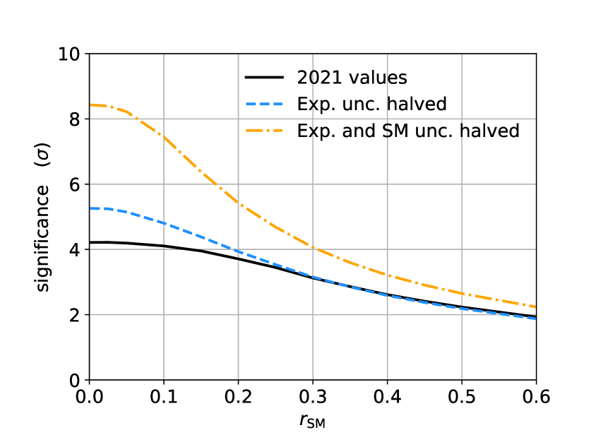
Figure 2: The significance of the muon $g-2$ discrepancy as a function of $r_{\rm SM}$ assuming the 2021 uncertainties (with SM uncertainty from [3]), with the experimental uncertainty reduced by a factor of two, and with the SM uncertainty also halved.

From Fig. 2 one sees that improved experimental accuracy is of almost no benefit unless the accuracy with which one assigns the SM uncertainty is kept below around 20% Also shown on the plot is the significance using an experimental uncertainty reduced by a factor of two and an SM uncertainty $\sigma_{\rm SM}$ halved from 0.43 to 0.215. The situation is improved somewhat by a reduction in the SM uncertainty, but still only if this uncertainty is itself assigned to correspond accurately to one standard deviation. If the naive recipe $\sigma_{\rm SM}\rightarrow(1+r_{\rm SM})\sigma_{\rm SM}$ is applied to the case of halved uncertainties one finds a significance of $6.6\sigma$ at $r_{\rm SM}=0.5$, compared to only $2.6\sigma$ from the gamma variance model.

5 Discussion and conclusions

It should not be a surprise that the significance of the discrepancy between SM prediction and experiment decreases when one supposes an additional source of uncertainty, namely, the “error on the error” represented by $r_{\rm SM}$. What is important to note, however, is that simply inflating the corresponding uncertainty by a factor of $(1+r_{\rm SM})$ does not adequately reflect the decrease in significance, as can seen by the curves in Fig. 1. Rather, the gamma variance model, which treats the assigned systematics as gamma-distributed estimates, results in a more rapid degradation of the significance for a relative uncertainty greater than a certain level, starting around 20% for this problem. If the relative uncertainty is 30%, then the significance drops to $3.1\sigma$, and it goes below $2\sigma$ for a relative uncertainty of 60%.

If the all of the nominal uncertainties are reduced by a factor of two relative to their current values, the discovery significance under assumption of $r_{\rm SM}=0$ is $8.4\sigma$. But this reduces to $5\sigma$ assuming a relative uncertainty in the theory error itself of 22%, and to $4\sigma$ for 30%. These results reflect the intrinsic difficulty in establishing a discovery at a high significance level if the uncertainties themselves are not accurately determined, and as a consequence the corresponding distributions acquire non-Gaussian tails. This underlines the importance of establishing appropriate procedures for quantifying systematic uncertainties both for the muon $g-2$ anomaly as well as for any investigations seeking to discover new phenomena.

References

- [1] B. Abi et al. (Muon Collaboration), Measurement of the Positive Muon Anomalous Magnetic Moment to 0.46 ppm, Phys. Rev. Lett. 126, 141801 (2021).
- [2] G. W. Bennett et al. (Muon Collaboration), Final report of the E821 muon anomalous magnetic moment measurement at BNL, Phys. Rev. D 73, 072003 (2006).
- [3] T. Aoyama, N. Asmussen, M. Benayoun, J. Bijnens, and T. Blum et al., The anomalous magnetic moment of the muon in the standard model, Phys. Rep. 887, 1 (2020).
- [4] G. Cowan, Statistical Models with Uncertain Error Parameters, Eur. Phys. J. C (2019) 79:133.
- [5] Sz. Borsanyi et al., Leading hadronic contribution to the muon magnetic moment from lattice QCD, Nature vol. 593, (2021) 51-55.
- [6] G. Cowan, Statistical Data Analysis, Oxford University Press, 1998.
- [7] K. Cranmer, Statistical challenges for searches for new physics at the LHC, in Proceedings of PHYSTAT05, L. Lyons and M.K. Unel (eds.), Imperial College Press, pp. 112-123 (2005).
- [8] P.A. Zyla et al. (Particle Data Group), Prog. Theor. Exp. Phys. 2020, 083C01 (2020).
- [9] M.S. Bartlett, Properties of sufficiency and statistical tests, Royal Society of London Proceedings Series A 160, (1937) 268-282.