Difference-in-Differences with a Continuous Treatment

This paper analyzes difference-in-differences setups with a continuous treatment. We show that treatment effect on the treated-type parameters can be identified under a generalized parallel trends assumption that is similar to the binary treatment setup. However, interpreting differences in these parameters across different values of the treatment can be particularly challenging due to selection bias that is not ruled out by the parallel trends assumption. We discuss alternative, typically stronger, assumptions that alleviate these challenges. We also provide a variety of treatment effect decomposition results, highlighting that parameters associated with popular linear two-way fixed-effect (TWFE) specifications can be hard to interpret, even when there are only two time periods. We introduce alternative estimation procedures that do not suffer from these TWFE drawbacks, and show in an application that they can lead to different conclusions.

JEL Codes: C14, C21, C23

Keywords: Difference-in-Differences, Continuous Treatment, Multi-Valued Discrete Treatment, Parallel Trends, Two-way fixed effects, Multiple Periods, Variation in Treatment Timing, Treatment Effect Heterogeneity

1 Introduction

The canonical difference-in-differences (DiD) research design compares outcomes between treated and untreated groups (difference one), before and after treatment started (difference two). But in many DiD applications, the treatment does not simply “turn on”, it has a “dose” or operates with varying intensity. Pollution dissipates across space, affecting locations near its source more severely than faraway locations. Localities spend different amounts on public goods and services, or set different minimum wages. Students choose how long to stay in school.

Continuous treatments can offer advantages over binary ones. Variation in intensity makes it possible to evaluate treatments that all units receive. A clear “dose-response” relationship between outcomes and treatment intensity can bolster the case for a causal interpretation or test a theoretical prediction. Finally, we may care more about the effect of changes in treatment intensity, such as increased funding, pollution abatement, or expanded eligibility, than about the effect of the existence of a treatment that already exists.

Despite how conceptually useful and practically common continuous DiD designs are, currently available econometric results provide little guidance on applying and interpreting them, except in some specific cases. In this paper, we introduce a set of tools that are suitable for DiD setups with variation in treatment dosage. In particular, we (a) discuss how one can identify a variety of treatment effect parameters by exploiting parallel-trends-type assumptions, (b) show that two-way fixed-effects (TWFE) estimators typically fail to have appealing causal interpretations, even when weights are non-negative, and (c) propose nonparametric estimators for clearly defined causal parameters that have attractive statistical properties, such as fast uniform convergence rates and narrow confidence bands. Our results cover DiD setups with varying treatment intensity or differential exposure to treatment but do not cover fuzzy designs.

We start by discussing causal parameters in a two-period DiD design in which units move from no treatment to a non-zero dose—we first focus on simple setups with two time periods to foster intuition and simplify exposition but later present extensions to more complex staggered designs with continuous treatments. We call the difference between a unit’s potential outcome under dose $d$ and its untreated potential outcome a level treatment effect. We call the difference in a unit’s potential outcome with a marginal increase in the dose a causal response [8]. When treatment is binary, these two notions of treatment effects coincide, but they do not under a continuous treatment. Importantly, level treatment effects and causal responses can have meaningfully different interpretations, and we establish that they require different identifying assumptions as well. Comparisons between treated and untreated units identify average (level) treatment effect parameters under a parallel trends assumption on untreated potential outcomes, similar to binary DiD designs. Comparisons between adjacent dose groups, however, do not identify average causal response parameters under the “standard” parallel trends assumption. We discuss an alternative but typically stronger assumption, which we call strong parallel trends, that says that the path of outcomes for lower-dose units must reflect how higher-dose units’ outcomes would have changed had they instead experienced the lower dose. Thus, strong parallel trends restricts treatment effect heterogeneity and justifies comparing dose groups. Absent this type of condition, comparisons across dose groups include causal responses but are “contaminated” by an additional term involving possibly different treatment effects of the same dose for different dose groups—we refer to this additional term as selection bias.

We next use the identification results to evaluate the most common way that practitioners estimate continuous DiD designs, which is to run a TWFE regression that includes time fixed effects ($\theta_{t}$), unit fixed effects ($\eta_{i}$), and the interaction of a dummy for the post-treatment period ($Post_{t}$) with a variable that measures unit $i$’s dose or treatment intensity, $D_{i}$:

$$Y_{i,t}=\theta_{t}+\eta_{i}+\beta^{twfe}D_{i}\cdot Post_{t}+v_{i,t}.$$ (1.1)

This TWFE specification is clearly motivated by DiD setups with two periods and two treatment groups, though many prominent textbooks recommend using it in more general setups (e.g., [16], [9], and [50]). There are several ways to interpret $\beta^{twfe}$, each corresponding to a different type of causal parameter. We decompose it in terms of level effects, scaled level effects, causal responses, and scaled high-versus-low ($2\times 2$) effects. Each decomposition is a weighted integral of dose-specific causal parameters, and none provide a clear causal and policy-relevant interpretation of $\beta^{twfe}$, at least not when treatment effects are allowed to vary across doses and/or groups.

For instance, we show that $\beta^{twfe}$ can be expressed as a weighted integral of average level treatment effect parameters but where the weights integrate to zero, indicating that $\beta^{twfe}$ should not be interpreted as an average (level) treatment effect. Interestingly, however, TWFE puts negative weights on the below-average dose units and positive weights on above-average dose units, and, thus, after re-scaling by a weighted average of the difference between doses for high- and low-dose units, is equivalent to a weighted binary DiD using higher-dose units as the “treated” group and lower-dose units as the “comparison” group, with weights proportional to a unit’s absolute distance from the mean dose. Our next decomposition, based on average level treatment effect parameters scaled by their dose, also displays negative weights, though their weights integrate up to one and not zero.

In contrast, a TWFE decomposition in terms of average causal response parameters has weights that integrate up to one and are non-negative, but also includes a selection bias term stemming from effect heterogeneity across doses. The strong parallel trends assumption eliminates this selection bias. The weights on causal responses at different doses, however, differ from the distribution of the dose, which creates a further challenge to interpreting $\beta^{twfe}$ in the presence of treatment effect heterogeneity, even if strong parallel trends holds. This is particularly important when the magnitude of the causal effects is of interest, but also has a strong bite in setups with nonlinear average level treatment effects, as average causal responses may have different signs across the dosage distribution. We reach a similar conclusion when decomposing $\beta^{twfe}$ using the scaled $2\times 2$ average effects as building blocks.

Given these drawbacks, we propose nonparametric DiD estimators that build on our identification results and recover interpretable causal parameters. When the treatment is discrete, this is as simple as running a linear regression with multiple treatment indicators, which is similar to staggered DiD setups [15]. When the treatment is continuous, we propose a modest adaption of [20] that allows us to estimate the average level treatment effects and the average causal responses as functions of the dose. These tools are motivated by clearly defined parallel trends assumptions, do not rely on strong functional form assumptions, are easy to implement, and are fully data-driven. It follows from [20] that our DiD estimators for continuous treatment converge at the fastest possible (i.e., minimax) rate in sup-norm, and our uniform confidence bands are asymptotically narrower (more precise) than those based on undersmoothing, and yet have correct asymptotic coverage and contract at, or within a $\log\log n$ factor of, the minimax rate. We also show how to construct causal summary measures of our average treatment effect functions that bypass the TWFE weighting problems by using the dose density as weights. Our results suggest that one can easily summarize average level treatment effects among treated units by comparing the average change in outcomes for all treated units to the average change in outcomes for untreated units [49]. This can be estimated by running a binary DiD with a “treatment dummy” equal to one for any units with positive doses. Summarizing average causal responses using dose density weights involves estimating an average derivative, which is simple to compute using “flexible” linear regressions. We also discuss how to construct event-study results using these summary measures, which can then be used to assess the plausibility of the parallel trends assumptions.

To show how TWFE regressions perform in practice and to illustrate the benefits of our proposed estimators, we revisit [1]’s acemoglu-finkelstein-2008 study of a 1983 Medicare reform that eliminated labor subsidies for hospitals. The original paper uses a TWFE estimator to compare the change in capital-labor ratios between hospitals whose input prices were more or less affected by the end of the subsidy. It concludes that price regulations favoring capital significantly increase capital use. The distinction between level treatment effect parameters and causal responses is important in this example: a positive level treatment effect shows that the policy as a whole increased the use of capital, while causal responses describe which subsidy levels generated the largest responses. We find that the reform raised capital-labor ratios by about 18 percent, which is 50 percent larger than the comparable TWFE estimate because of the weighting issues highlighted by our decompositions. We also estimate variable average causal response ($ACR$) parameters that are quite large at low subsidy levels—implying elasticities of substitution greater than 2—yet slightly negative for most positive doses. These negative $ACR$ estimates cast doubt on the strong parallel trends assumption, the simple two-factor model of hospital production, or both. Our results support [1]’s acemoglu-finkelstein-2008 conclusion that the 1983 Medicare reform led hospitals to favor capital over labor, but suggests caution in a policy interpretation about which subsidy levels have the largest effects or an economic interpretation in terms of production function parameters.

Related Literature: This paper contributes to the fast-growing literature on modern DiD methods; see, e.g., [44], [28], and [14] for overviews. Most of this work focuses on binary treatment setups, with a few exceptions. [25] focuses on fuzzy designs, where a researcher is interested in individual-level effects of a binary treatment that has been aggregated across units into a continuous “treatment rate.” In contrast, we study “sharp” designs where the treatment exposure is itself continuous or multi-valued discrete at the unit-level. The supplemental appendix of [26] considers the case with ordered multi-valued treatments and presents a decomposition of TWFE regressions using a scaled treatment effect measure as the “building block.” Our decomposition differs from theirs in that we allow for continuous treatments and also consider different building blocks. See also [24] for Changes-in-Changes-types of procedures with a continuous treatment in the spirit of [11].

In work subsequent to ours, [27] consider a DiD setup with continuous treatments with potentially non-staggered (but static) treatments. Their paper and ours tackle related but different and complementary problems. For instance, their target parameters differ from ours, as they consider (distance-weighted) averages of what we refer to as $2\times 2$ average effects. Unlike our $ACR$, these parameters average effects of discrete rather than marginal changes of treatments. Furthermore, our estimation procedures greatly differ from theirs, as we consider both functional parameters (dose-response and $ACR$ curves) and causal summary measures. On the other hand, they consider instrumental variable extensions, which we do not.

Our TWFE decompositions are related to a number of recent results on the limitations of TWFE linear regressions in the presence of treatment effect heterogeneity. For example, that some of our TWFE decompositions include negative weights is related to the negative weights that can arise for TWFE estimators with binary treatments (see, e.g., [32], [26], [48], and [13]). We add to this literature by highlighting that the same TWFE regression coefficient can have different interpretations depending on the “building blocks”, and that new “bias” terms may appear, depending on the type of parallel trends assumption being used. Although our results show that negative weights can show up even in the two-period cases, which is not the case in the papers above, a perhaps more important lesson from our decompositions is that even when all weights are non-negative, TWFE can still provide an unappealing causal summary parameter with heterogeneous treatment effects. We also note that, as a by-product of our decomposition results, if one replaces our DiD setting with one with cross-sectional data and a randomly assigned dose, all four of our decomposition results would continue to go through (e.g., just take the pre-treatment outcome to be zero almost surely), highlighting that linear specifications may not be very attractive with continuous treatments, even when the dose is fully randomized. These results seem to be new to the literature.

To construct our new DiD estimators and conduct asymptotically valid (data-driven) inferences, we build on [20]; see also [21, 22]. More specifically, we adapt [20]’s nonparametric IV data-driven sup-norm adaptive estimation and inference procedures to our context. Doing so allows us to estimate the average level treatment effect and the average causal response curves in a single shot, at least under strong parallel trends. We also show how one can build on these estimators to get easy-to-interpret summary treatment effect measures. This feature of our paper connects to the literature on the efficient estimation of average derivatives, examples of which include [40], [3], [19] and references therein.

Our results are also related to other branches of causal inference and econometrics. For instance, [31] connect Bartik instruments to DiD designs under an independence assumption. We complement this analysis by studying identification in a similar setup under different kinds of parallel trends assumptions. Our cautionary results about interpreting comparisons of $ATT$s at different doses echo related points on comparing “local” treatment effect parameters to each other. Some examples include [42, 6, 38] in the context of local average treatment effects; [18] and [17] in the context of regression discontinuity designs with multiple cutoffs; or [29] in the context of difference-in-differences with two treatments. Our results highlighting limitations of linear regressions to approximate treatment effects are related to [10], [46, 47], [12], and [30]. In particular, our decomposition results about the importance of the building block parameters are related to [46], which also discusses related points in binary cross-sectional designs based on unconfoundedness. Finally, we note that our causal response decomposition builds on [51, Proposition 2 ], which expresses the slope coefficient in a regression of an outcome on a continuous variable as a weighted average of underlying local slopes. Besides differences related to causal interpretations and panel data, we extend those results to allow for a mass of untreated units.

2 Motivating Continuous DiD from an Empirical Perspective

To fix ideas and provide intuition for our theoretical results, we revisit [1]’s acemoglu-finkelstein-2008 (AF) study of how price regulations affect firms’ input choices. When Medicare began in 1965, hospitals received reimbursements from the federal government for a share of their labor and capital expenditures proportional to the fraction of total patient days accounted for by Medicare recipients ($m_{i}$). Hospital $i$ thus faced input prices equal to $(1-s_{L}m_{i})w$ for labor and $(1-s_{K}m_{i})r$ for capital, where $s_{L}$ and $s_{K}$ are the labor and capital subsidy rates and $w$ and $r$ are market wages and rental rates. In 1983, Medicare moved to the Prospective Payment System (PPS), which replaced the labor subsidy with a small payment per episode/diagnosis. This set $s_{L}=0$ but left the capital subsidy unchanged. Therefore, the price of labor for a given hospital rose from $(1-s_{L}m_{i})w$ to $w$, skewing relative factor prices.

The statutory relationship between a hospital’s Medicare volume, $m_{i}$, and the change in its price of labor, $s_{L}m_{i}w$, motivates AF’s use of a continuous DiD design comparing changes in capital/labor ratios before and after 1983 between hospitals with different pre-PPS Medicare inpatient shares. AF’s description, estimation, and interpretation of this empirical strategy touch on some of the most common ways of justifying and implementing continuous DiD designs.

One motivation for this design is practical: variation in a dose (or exposure) permits the evaluation of treatments for which binary DiD is either infeasible or undesirable. In AF’s case, about 15 percent of hospitals were “untreated” by the change in Medicare’s subsidy policy because they served non-Medicare-eligible populations, like children or psychiatric patients, so they may not constitute a valid comparison group. AF therefore describe $m_{i}$, which is the hospital’s Medicare volume in 1983, as an “attractive source of variation” in the price of labor both because it varies substantially—the mean of $m_{i}$ among treated hospitals is 0.45, and the standard deviation is 0.15—and because hospitals with $m_{i}>0$ may be more comparable to each other than treated hospitals are to untreated hospitals.

Another common justification for continuous DiD designs is that a “dose-response” relationship between exposure and outcomes can support a causal interpretation or test a theoretical prediction. [37, p. 158 ], for example, argues that “differences in the intensity of the treatment across different groups allow one to examine if the changes in outcomes differ across treatment levels in the expected direction.” AF lay out a simple theoretical framework in which the move to PPS should (i) raise capital/labor ratios and (ii) do so more strongly for hospitals with higher pre-PPS values of $m_{i}$. They view their continuous DiD design as a way to estimate a causal effect of PPS as a whole and test the theoretical predictions of their model.

Finally, researchers often advocate for continuous DiD designs because they can be used to estimate average causal effects of small changes in the dose. In many economic models, price and income elasticities determine optimal policies like tax rates, tax bases, subsidies, and regulations [33], but these are continuous concepts that can be estimated accurately only with continuous variation. We discuss how AF’s theoretical framework implies, under some assumptions, that DiD estimates provide information about hospitals’ elasticity of substitution between capital and labor, although AF do not argue for this kind of “marginal” interpretation.

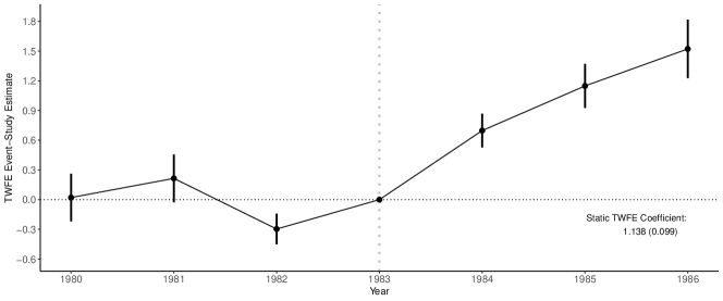
Figure 1: Two-Way Fixed Effects Event-Study Estimates of the Effect of Medicare’s Reimbursement Reform on Hospital Input Mix

Notes: The figure plots TWFE event-study coefficients and their 95% confidence intervals from regressions with hospital fixed effects, year fixed effects, and the 1983 Medicare inpatient share ($m_{i}$) interacted with either a dummy for years after 1983 or the year dummies. The outcome variable is the depreciation share of total operating expenses, a measure of hospitals’ capital/labor ratio. The data cover the years 1980-1986 and come from the American Hospital Association’s annual survey [4]. We dropped 860 hospitals (out of 6741) that have missing data for the outcome. We also report the static TWFE coefficient and standard errors associated with (1.1). All standard errors are clustered at the hospital level.

In terms of estimation, AF use the standard tool for continuous DiD designs: a TWFE regression with hospital and year fixed effects. They follow textbook advice. [50, p. 132 ] observes that a two-period DiD regression estimator “can be easily modified to allow for continuous, or at least non-binary, ‘treatments.”’ [9, p. 234 ] emphasize “a second advantage of regression DD is that it facilitates the study of policies other than those that can be described by a dummy.” They also follow common practice and describe their identifying assumption as an extension of the parallel trends assumption from binary designs: “Without the introduction of PPS, hospitals with different $m_{i}$’s would not have experienced differential changes in their outcomes in the post-PPS period” (emphasis added).

Figure 1 reproduces AF’s DiD event-study coefficients for each calendar year, relative to 1983, and the estimate of $\beta^{twfe}$ from an equation like (1.1). AF interpret these results as indicative that after 1983, capital/labor ratios rose more strongly for hospitals with higher values of $m_{i}$, without a substantial differential change in input mix before PPS. Our impression is that event-study results like those in Figure 1 would usually be interpreted as strong causal evidence because there are (relatively) small pre-trend estimates, large differences in outcomes between higher- and lower-dose units after treatment, and tight confidence intervals. What is missing from most continuous DiD analyses, however, is a specific statement about what causal parameters researchers would like to estimate, the assumptions under which they are identified, and a formal justification for a particular estimator. Our goal is to shed light on these three issues.

3 Baseline Case: A New Treatment with Two Periods

We illustrate our main points in a setup with two periods of panel data, $t=1$ and $t=2$. In the second period, some units receive a treatment “dose,” denoted by $D_{i}$, and others remain untreated. Extensions to multiple periods and staggered setups are discussed in Section 5. We denote the support of $D$ by $\mathcal{D}$. $D_{i}$ can be (absolutely) continuous or can be multi-valued discrete, but to simplify the exposition, we refer to it as “continuous.” We define potential outcomes for unit $i$ in period $t$ as $Y_{i,t}(d)$. This is the outcome that unit $i$ would experience in period $t$ under dose $d$. In each time period $t$, the observed outcome for unit $i$ is $Y_{i,t}=Y_{i,t}(D_{i})$. We assume that all expectations are finite and well-defined. Henceforth, we omit the unit index $i$ to make the notation less cluttered and define $\Delta Y=Y_{t=2}-Y_{t=1}$.

3.1 Parameters of Interest with a Continuous Treatment

The potential outcomes notation $Y_{t}(d)$ reflects that treatment can take many values, and so each unit can experience many types of causal effects. The level treatment effect of dose $d$ in time period $t$ for a given unit is defined as its potential outcome when $D=d$ minus its untreated potential outcome: $Y_{t}(d)-Y_{t}(0)$. Level treatment effects measure the treatment effect at time $t$ from switching treatment dosage from $0$ to $d$. This is a straightforward extension of a binary “treatment effect” to a continuous “treatment effect function” or “dose-response function.”

But zero-treatment is not the only relevant counterfactual. We define a unit’s causal response at $d$ as $Y_{t}^{\prime}(d)$, the derivative of the potential outcome with respect to dose $d$ (when the treatment is continuous), or as the difference in potential outcomes between adjacent doses, $Y_{t}(d_{j})-Y_{t}(d_{j-1})$ (when the treatment is discrete). Causal responses measure the treatment effect at time $t$ of a “marginal” increment of dose $d$. These two types of treatment effects—the level of $Y_{t}(d)-Y_{t}(0)$ or its slope, $Y^{\prime}_{t}(d)$—define unit-level causal parameters in continuous designs, and connect to results in the instrumental variables (IV) literature on multi-valued discrete or continuous endogenous variables ([8], [7]).

We focus on “building block” parameters that are averages of these two kinds of causal effects in the post-treatment period, $t=2$. Average level treatment effects (which we refer to as average treatment effects) extend definitions from the binary case:

$$ATT(d|d^{\prime})=\mathbb{E}[Y_{t=2}(d)-Y_{t=2}(0)|D=d^{\prime}]\quad\textrm{and}\quad ATE(d)=\mathbb{E}[Y_{t=2}(d)-Y_{t=2}(0)],$$

where $ATT(d|d^{\prime})$ is the average effect of dose $d$ compared to zero dosage in the post treatment period $t=2$, on units that actually experienced dose $d^{\prime}$. When $d^{\prime}=d$, this is the $ATT$ among units that received dose $d$. $ATE(d)$ is the average difference between potential outcomes under dose $d$ relative to untreated potential outcomes across all units, not just those that experienced dose $d$, in time period $t=2$.

Average causal response parameters for absolutely continuous treatments are defined as

$$ACRT(d|d^{\prime})=\frac{\partial ATT(l|d^{\prime})}{\partial l}\bigg{|}_{l=d}=\frac{\partial\mathbb{E}[Y_{t=2}(l)|D=d^{\prime}]}{\partial l}\bigg{|}_{l=d}\textrm{ and }ACR(d)=\frac{\partial ATE(d)}{\partial d}=\frac{\partial\mathbb{E}[Y_{t=2}(d)]}{\partial d}.$$

$ACRT(d|d)$ equals the derivative of the $t=2$ average potential outcome for units that received dose $d$ evaluated at $d$. This is equivalent to the derivative of $ATT(l|d)$ with respect to $l$, evaluated at $l=d$. For discrete treatments, average causal responses are defined in a similar way but with slightly different notation to accommodate discreteness of $d$:

$$ACRT(d_{j}|d_{k})=\mathbb{E}[Y_{t=2}(d_{j})-Y_{t=2}(d_{j-1})|D=d_{k}]\quad\textrm{and}\quad ACR(d_{j})=\mathbb{E}[Y_{t=2}(d_{j})-Y_{t=2}(d_{j-1})].$$

$ACRT(d_{j}|d_{j})$ equals the difference in mean potential outcomes between dose level $d_{j}$ and the next lowest dose $d_{j-1}$ in period $t=2$. We follow the literature, particularly [8], by not defining $ACRT(d_{j}|d_{j})$ as being scaled by the difference between $d_{j}$ and $d_{j-1}$ though, up to definitions of parameters, that does not affect the results below.

Figure 2: Causal Parameters in a Continuous Difference-in-Differences Design

Notes: The figure plots $ATT(\cdot|d)$ (the average effect of experiencing each dose among units that actually experienced dose $d$). We highlight causal parameters for two doses, $d$ and $d^{\prime}$. $ATT(d|d)$ and $ATT(d^{\prime}|d)$ are average treatment effect on the treated parameters and refer to the height of the curve. $ACRT(d|d)$ and $ACRT(d^{\prime}|d)$ are average causal response parameters and refer to the slope of the curve. We show them for a continuous dose, when the $ACRT$ is a tangent line, and for a discrete dose when $ACRT$ is a line connecting two discrete points on $ATT(D|d)$.

Figure 2 illustrates these parameters graphically. The concave line plots an average treatment effect function against the dose for units actually treated with dose $d$, $ATT(\cdot|d)$. If we consider dose levels $d$ and $d^{\prime}$, there are two possible $ATT$ parameters. The first, $ATT(d|d)$, the level of group $d$’s average treatment effect function at $d$, is an average treatment effect that is “local” to units that experienced dose $d$. The second, $ATT(d^{\prime}|d)$, is also “local” to the $d$ group, but refers to the effect they would experience at dose $d^{\prime}$ even though they did not actually receive that dose. The continuous-dose $ACRT$ parameters are the slopes of tangent lines to the $ATT(\cdot|d)$ function, and the discrete-dose $ACRT$ parameters are the slopes of lines connecting two points on the $ATT(\cdot|d)$ function. As with $ATT$s, our definitions encompass causal responses to doses other than the one a group actually receives (i.e., $ACRT(d^{\prime}|d)$).

A proper interpretation of continuous DiD results hinges on which type of parameter one wants, and can identify and estimate. For instance, even if all $ATT(d|d)$ parameters are large and positive, some $ACRT(d|d)$ parameters could be zero or negative. A researcher misinterpreting a large $ATT$ estimate as an $ACR$, in this case, would mistakenly conclude that a policy to raise every unit’s dose would have large effects. A researcher confusing a small $ACR$ for an $ATT$ would mistakenly conclude that an entire policy was ineffective, even though it actually just has small effects at the margin.

The above-mentioned causal parameters are functional parameters because they are allowed to vary arbitrarily across dose groups $d$ and across (counterfactual) doses $d^{\prime}$. This contrasts with $\beta^{twfe}$ from (1.1), which is a single number. In practice, we expect researchers to also typically want to aggregate these functional parameters into lower-dimensional objects that are easier to report and may be more precisely estimated. We focus on aggregating the functional parameters discussed above by averaging them using the distribution of the dose among all treated units. We denote these summary parameters by

$$ATT^{o}=\mathbb{E}[ATT(D|D)|D>0]\qquad\textrm{and}\qquad ATE^{o}=\mathbb{E}[ATE(D)|D>0]$$

$$ACRT^{o}=\mathbb{E}[ACRT(D|D)|D>0]\qquad\textrm{and}\qquad ACR^{o}=\mathbb{E}[ACR(D)|D>0].$$

These provide natural ways to summarize the underlying parameters; moreover, all four of these parameters provide “best” approximations in the sense of minimizing the mean squared distance between the summary parameter and the functional parameters. Also, note that $ACRT^{o}$ and $ACR^{o}$ are average derivative-type parameters, and average derivatives have been widely studied in econometrics, see, e.g., [40], [3], [19], and references therein.

3.2 Identification with a Continuous Treatment

This section discusses the identification of average treatment effect and average causal response parameters. Toward this end, we make the following assumptions.

Assumption 1 (Random Sampling).

The observed data consist of $\{Y_{i,{t=2}},Y_{i,t=1},D_{i}\}_{i=1}^{n}$, which is independent and identically distributed.

Assumption 2 (Continuous or Multi-Valued Discrete Treatment).

In period $t=1$, no unit is treated, while in period $t=2$, the treatment dosage $D$ has support $\mathcal{D}=\{0\}\cup\mathcal{D}_{+}$ and is either continuous or multi-valued discrete. More precisely, one of the following is true:

• $\mathcal{D}_{+}=\mathcal{D}_{+}^{c}$, where $\mathcal{D}_{+}^{c}=[d_{L},d_{U}]$ with $0<d_{L}<d_{U}<\overline{d}<\infty$, for some $\overline{d}\in\mathbb{R}$. In addition, $\mathbb{P}(D=0)>0$, $f_{D|D>0}$ is a Lebesgue density which satisfies $a_{f}^{-1}<f_{D|D>0}(d)<a_{f}$ for some positive constant $a_{f}<\infty$ and all $d\in\mathcal{D}_{+}^{c}$, and $\mathbb{E}[\Delta Y|D=d]$ is continuously differentiable on $\mathcal{D}_{+}^{c}$.

• $\mathcal{D}_{+}=\mathcal{D}_{+}^{mv}$ where $\mathcal{D}_{+}^{mv}=\{d_{1},d_{2},\ldots,d_{J}\}$ where $0<d_{1}<d_{2}<\cdots<d_{J}<\overline{d}<\infty$, for some $\overline{d}\in\mathbb{R}$. In addition, $\mathbb{P}(D=d)>0$ for all $d\in\mathcal{D}$.

Assumption 3 (No-Anticipation and Observed Outcomes).

For all units, and all $d\in\mathcal{D}$,

$$Y_{i,t=1}=Y_{i,t=1}(d)=Y_{i,t=1}(0)\quad\textrm{and}\quad Y_{i,t=2}=Y_{i,t=2}(D_{i}).$$

Assumption 1 says that we observe two periods of $iid$ panel data. Assumption 2 formalizes that a mass of units do not participate in the treatment in either period (we discuss the case with no untreated units in more detail at the end of this section), and the rest receive a continuous (2a) or discrete (2b) treatment. Assumption 2a allows for the smallest value of the treatment to be strictly larger than zero, which is common in applications. Assumption 3 says that units do not anticipate future treatments, so we observe untreated potential outcomes for all units in the first period. In the second period, we observe the potential outcome corresponding to the actual dose that unit $i$ experienced.

3.2.1 Identification under parallel trends

Identification of average level treatment effects follows closely from the DiD setup with binary treatments. In particular, our results rely on an extension of the binary parallel trends assumption.

Assumption 4 (Parallel Trends).

For all $d\in\mathcal{D}$,

$$\mathbb{E}[Y_{t=2}(0)-Y_{t=1}(0)|D=d]=\mathbb{E}[Y_{t=2}(0)-Y_{t=1}(0)|D=0].$$

Assumption 4 says that the average evolution of outcomes that units with any dose $d$ would have experienced without treatment is the same as the evolution of outcomes that units in the untreated group actually experienced. Binary DiD designs also rely on assumptions like this. To simplify the exposition below, we often simply refer to Assumption 4 as parallel trends (PT). The following result shows that under Assumption 4, $ATT(d|d)$ is identified; all proofs are in Appendix B.

Theorem 3.1.

Under Assumptions 1, 2, 3 and 4, $ATT(d|d)$ is identified for all $d\in\mathcal{D}_{+}$, and it is given by

$$ATT(d|d)=\mathbb{E}[\Delta Y|D=d]-\mathbb{E}[\Delta Y|D=0].$$

Furthermore, $ATT^{o}=\mathbb{E}[\Delta Y|D>0]-\mathbb{E}[\Delta Y|D=0]$.

The identification results for $ATT(d|d)$ in Theorem 3.1 hold by essentially the same arguments used for binary treatments. Because Assumption 4 ensures that $\mathbb{E}[\Delta Y|D=0]$ is the same as the evolution of outcomes that treated units would have experienced without the treatment, $ATT(d|d)$ equals the difference between the change in outcomes for the dose $d$ group and the untreated group. As a direct consequence, by averaging all the $ATT(d|d)$s over the distribution of non-zero dosages, we have that the summary parameter $ATT^{o}$ is identified by simply comparing units with a positive dose to untreated units. On the other hand, parallel trends, as defined in Assumption 4, is not strong enough to guarantee the identification of $ATE(d)$; this issue is also present in binary setups.

The identification of average causal response parameters differs from the identification of $ATT$ parameters because it requires comparisons between dose groups. Our central identification result is that causal response parameters are not identified under Assumption 4, because comparisons between different dose groups are biased when treatment effects (of the same dose) vary across dose groups, even when the average evolution of untreated potential outcomes is the same.

Theorem 3.2.

Under Assumptions 1, 2, 3 and 4, causal response parameters are not identified. Specifically,

• Under Assumption 2(a), for $d\in\mathcal{D}_{+}^{c}$,

  $$\frac{\partial\mathbb{E}[\Delta Y|D=d]}{\partial d}=\frac{\partial ATT(d|d)}{\partial d} =ACRT(d|d)+\underbrace{\frac{\partial ATT(d|l)}{\partial l}\Big{|}_{l=d}}_{\textrm{selection bias}};$$

• For $(h,l)\in\mathcal{D}\times\mathcal{D}$,

  $$\mathbb{E}[\Delta Y|D=h]-\mathbb{E}[\Delta Y|D=l] =ATT(h|h)-ATT(l|l)$$

  $$=\underbrace{\mathbb{E}[Y_{t=2}(h)-Y_{t=2}(l)|D=h]}_{\textrm{causal response}}+\underbrace{\Big{(}ATT(l|h)-ATT(l|l)\Big{)}}_{\textrm{selection bias}}.$$

  When Assumption 2(b) holds, taking $h=d_{j}$ and $l=d_{j-1}$ implies that

  $$\mathbb{E}[\Delta Y|D=d_{j}]-\mathbb{E}[\Delta Y|D=d_{j-1}] =ACRT(d_{j}|d_{j})+\underbrace{ATT(d_{j-1}|d_{j})-ATT(d_{j-1}|d_{j-1})}_{\textrm{selection bias}}.$$

Theorem 3.2 says that under parallel trends, comparisons of outcome paths between higher- and lower-dose groups mix together (i) causal responses and (ii) a “selection bias” type of term that comes from differences in average treatment effects of the same dose for different dose groups. Intuitively, even if untreated potential outcomes evolve in the same way, observed paths of outcomes differ between dose groups for two reasons. One is the causal response itself, which comes from differences in doses ($h$ versus $l$) causing differences in outcomes. The other is a selection bias type of contamination, which comes from differences across dose groups in the average level effect of the particular dose $l$—parallel trends does not rule out that different dose groups could experience different treatment effects of the same dose.

Figure 3: Non-identification of Average Causal Response with Treatment Effect Heterogeneity, Two Discrete Doses

Notes: The figure shows that comparing adjacent $ATT(d|d)$ estimates equals an $ACRT$ parameter (the slope of the higher-dose group’s $ATT$ function) and selection bias (the difference between the two groups’ $ATT$ functions at the lower dose).

Figure 3 illustrates this result for an example with two groups and two doses: $d$ and $d^{\prime}=d+1$. The slope of the line that connects the points $(d,ATT(d|d))$ and $(d^{\prime},ATT(d^{\prime}|d^{\prime}))$ is steeper than the average causal response of interest, $ACRT(d^{\prime}|d^{\prime})$, because it jumps from one $ATT$ function to the other. This is captured by the selection bias term, a version of selection-on-gains that equals the difference in treatment effects at the lower dose: $ATT(d|d^{\prime})-ATT(d|d)$. It breaks the causal interpretation because observed outcomes for lower-dose units are not a valid counterfactual for what higher-dose units would have experienced at a lower dose. The selection bias is not identified as we do not observe $Y_{t=2}(d)$ for units that experienced dose $d^{\prime}$. Such a result precludes a causal interpretation of $ATT$ differences across doses, at least when one is not willing to further strengthen parallel trends as defined in Assumption 4.

3.2.2 Identification under strong parallel trends

The fact that average causal responses are not identified under a traditional parallel trends assumption suggests that learning about this type of parameter with continuous DiD designs requires new assumptions as well. This section discusses an alternative, typically stronger assumption that allows for the identification of $ACR$ (and $ATE$) parameters, which we refer to as strong parallel trends (SPT).

Assumption 5 (Strong Parallel Trends).

For all $d\in\mathcal{D}$,

$$\mathbb{E}[Y_{t=2}(d)-Y_{t=1}(0)]=\mathbb{E}[Y_{t=2}(d)-Y_{t=1}(0)|D=d].$$

Under Assumption 3, the right-hand side of the equation in Assumption 5 is the (observed) average evolution of outcomes for dose group $d$. Assumption 5 says that the average evolution of outcomes for the entire population if all experienced dose $d$ (the left-hand side of the previous equation) is equal to the path of outcomes that dose group $d$ actually experienced. Assumption 5 notably differs from Assumption 4 because it involves potential outcomes under different doses, $Y_{t}(d)$, rather than only untreated potential outcomes, $Y_{t}(0)$.

An alternative way to think about Assumption 5 is as an assumption that restricts treatment effect heterogeneity. In Theorem C.1 in Appendix C, we show that if one maintains Assumption 4, Assumption 5 is equivalent to assuming that $ATT(d|d)=ATE(d)$ for all doses. While this condition does not impose full treatment effect homogeneity, it does rule out selection-on-gains into a particular dose group and ensures the observed outcome changes for every dose group reflect what would have happened to all other groups had they received that dose. This condition can also be viewed as a structural assumption in the sense that it effectively allows one to extrapolate treatment effects of dose $d$ among dose group $d$ to treatment effects of dose $d$ for the entire population.

In the remainder of this section, we show that Assumption 5 is useful for recovering “global” average causal effect parameters, which are straightforward to compare to each other, and, hence, sidestep the selection bias issues discussed above. Before doing that, it is worth mentioning that we are not proposing Assumption 5 as an assumption that empirical researchers should readily adopt; in fact, in many applications, Assumption 5 may be a strong or implausible assumption. Rather, our aim is to clarify that many natural target parameters in DiD applications with a continuous treatment require stronger assumptions than parallel trends as defined in Assumption 4.

Theorem 3.3.

Assume that Assumptions 1, 2, 3 and 5 hold.

• For $d\in\mathcal{D}_{+}$, it follows that

  $$ATE(d)=\mathbb{E}[\Delta Y|D=d]-\mathbb{E}[\Delta Y|D=0].$$

• When Assumption 2(a) holds (i.e., treatment is continuous), it follows that, for $d\in\mathcal{D}_{+}^{c}$,

  $$ACR(d)=\frac{\partial\mathbb{E}[\Delta Y|D=d]}{\partial d}=\frac{\partial ATE(d)}{\partial d},$$

• For $(h,l)\in\mathcal{D}\times\mathcal{D}$,

  $$ATE(h)-ATE(l)=\mathbb{E}[Y_{t=2}(h)-Y_{t=2}(l)]=\mathbb{E}[\Delta Y|D=h]-\mathbb{E}[\Delta Y|D=l]$$

  When Assumption 2(b) holds (i.e., treatment is discrete), by taking $h=d_{j}$ and $l=d_{j-1}$,

  $$ACR(d_{j})=\mathbb{E}[\Delta Y|D=d_{j}]-\mathbb{E}[\Delta Y|D=d_{j-1}]$$

For part (a) of Theorem 3.3, recall that $ATT(d|d)$ and $ATE(d)$ differ when there is selection into dose group $d$ on the basis of treatment effects. Strong parallel trends rules out that kind of selection, which means that comparing average outcome changes of dose group $d$ to the untreated group identifies $ATE(d)$. For parts (b) and (c), the same implication of strong parallel trends ensures that lower-dose groups are valid counterfactuals for higher-dose groups.

Strong parallel trends only changes the interpretation of the estimand, not its form. One important implication is that conventional pre-tests for differential changes across groups before treatment cannot distinguish between Assumption 4 and Assumption 5. Because only untreated potential outcomes are observed before treatment, these periods cannot test the additional content of an assumption like SPT that necessarily involves treated potential outcomes.

Finally, the identification results in Theorem 3.3 immediately imply that averages of the $ATE(d)$ and $ACR(d)$ building blocks are identified as well. The following corollary states these results.

Corollary 3.1.

Assume that Assumptions 1, 2, 3 and 5 hold.

• For $d\in\mathcal{D}_{+}$, it follows that

  $$ATE^{o}=\mathbb{E}[\Delta Y|D>d]-\mathbb{E}[\Delta Y|D=0].$$

• When Assumption 2(a) holds (i.e., treatment is continuous), it follows that, for $d\in\mathcal{D}_{+}^{c}$,

  $$ACR^{o}=\mathbb{E}\left[\left.\frac{\partial\mathbb{E}[\Delta Y|D=d]}{\partial d}\bigg{|}_{d=D}\right|D>0\right]=\int_{d_{L}}^{d_{U}}\frac{\partial\mathbb{E}[\Delta Y|D=d]}{\partial d}\bigg{|}_{d=s}f_{D|D>0}(s)ds.$$

• When Assumption 2(b) holds (i.e., treatment is multi-valued), it follows that, for $d_{j}\in\mathcal{D}_{+}^{mv}$,

  $$ACR^{o}=\sum_{j=1}^{J}\left(\mathbb{E}[\Delta Y|D=d_{j}]-\mathbb{E}[\Delta Y|D=d_{j-1}]\right)\mathbb{P}(D=d_{j}|D>0).$$

These results highlight how identification in continuous DiD designs is fundamentally a question about dose-specific building block parameters and the underlying parallel trends assumption, not the aggregation choices that lead to particular summary parameters.

Remark 3.1 (No untreated units).

Researchers often use continuous designs when all units in their sample receive some amount of the treatment having in mind comparing units that are “more treated” to units that are “less treated”. Without untreated units, it is infeasible to compare dose group $d$ to an untreated group, and, hence, it is infeasible to directly recover $ATT(d|d)$ or $ATE(d)$. However, a natural alternative is to compare dose group $d$ to dose group $d_{L}$ (the lowest possible amount of the treatment). In LABEL:app:no-untreated-units in the Supplementary Appendix, we show that, under parallel trends, when there are no untreated units,

$$\mathbb{E}[\Delta Y|D=d]-\mathbb{E}[\Delta Y|D=d_{L}]=ATT(d|d)-ATT(d_{L}|d_{L}).$$

This shows that this comparison is related to underlying causal effect parameters under parallel trends; however, recall from Theorem 3.2 that the expression on the right-hand side mixes together the average causal response of moving from $d_{L}$ to $d$ with selection bias. Under strong parallel trends, we have instead that

$$\mathbb{E}[\Delta Y|D=d]-\mathbb{E}[\Delta Y|D=d_{L}]=ATE(d)-ATE(d_{L})=\mathbb{E}[Y_{t=2}(d)-Y_{t=2}(d_{L})],$$

which does not include selection bias terms. This discussion highlights that (unlike a setting with a binary treatment) continuous variation in the dose can be used to learn about causal effects even if there is no untreated comparison group, but interpreting these results as causal effects of the treatments requires strengthening Assumption 4.

Remark 3.2 (Comparison between different parallel trends assumptions).

A researcher may be interested in comparing what is and what is not identified under different parallel trends assumptions, how these parallel trends assumptions restrict treatment effect heterogeneity, and how they compare to each other. In Appendix C, we pursue this exercise and provide a Portmanteau-type theorem that allows us to better understand the “bite” of each assumption. Among other things, we show that, in general, Assumption 4 and Assumption 5 are non-nested, though Assumption 5 will probably be stronger in most applications. We also introduce an aggregated parallel trends assumption that is useful for directly targeting $ATT^{o}$, and an alternative strong parallel trends assumption that implies both Assumption 4 and Assumption 5 but further restricts treatment effect heterogeneity. See Theorem C.1 for additional details.

3.3 What Parameter Does TWFE Estimate?

In practice, empirical researchers using a continuous DiD design typically estimate a single summary parameter using a TWFE regression like Equation 1.1. This section links the TWFE estimand to our identification results for dose-specific parameters, describes the assumptions necessary to give TWFE some causal interpretation, and discusses what that interpretation is. We focus on continuous treatments and defer the discussion of multi-valued discrete treatments to LABEL:app:twfe-multivalued-treatment in the Supplementary Appendix.

Our impression is that empirical researchers typically interpret $\beta^{twfe}$ in three main (and related) ways, implicitly relying on different building blocks. First, $\beta^{twfe}$ is often directly interpreted as a causal response parameter; that is, how much the outcome causally increases on average when the treatment increases by one unit. This is the causal version of how regression coefficients are often taught to be interpreted in introductory econometrics classes. Second, it is common to pick a representative value for $d$, to report $d\times\beta^{twfe}$, and interpret this quantity as $ATT(d)$. This is the main interpretation provided in [1]: “Given that the average hospital has a 38 percent Medicare share prior to PPS, this estimate [i.e., of $\beta^{twfe}$, here equal to 1.129] suggests that in its first 3 years, the introduction of PPS was associated with an increase in the depreciation share of about 0.42 ($\approx$ 1.129 $\times$ 0.38) for the average hospital.” Rearranging this expression shows that under this interpretation $\beta^{twfe}=ATT(d|d)/d$, which relates $\beta^{twfe}$ to a scaled level effect. Third, it is common to take two different representative values of the dose, $d_{1}$ and $d_{2}$—a common choice is the 25th percentiles and 75th percentiles of the dose—and interpret $\beta^{twfe}$ as the average causal response of moving from dose $d_{1}$ to dose $d_{2}$ scaled by the distance between $d_{1}$ and $d_{2}$; this is a scaled $2\times 2$ effect. We aim to assess whether such types of interpretations are justified and under which conditions.

Table 1: TWFE Decomposition Weights

Decomposition	$D>0$ Weights			$D=0$ Weights
Causal response	$w^{\textrm{acr}}_{1}(l)$	$=$	$\displaystyle\frac{(\mathbb{E}[D|D\geq l]-\mathbb{E}[D])\mathbb{P}(D\geq l)}{\mathrm{Var}(D)}$	$w^{\textrm{acr}}_{0}$	$=$	$\displaystyle\frac{(\mathbb{E}[D|D>0]-\mathbb{E}[D])\mathbb{P}(D>0)d_{L}}{\mathrm{Var}(D)}$
Levels	$w_{1}^{\textrm{lev}}(l)$	$=$	$\displaystyle\frac{(l-\mathbb{E}[D])}{\mathrm{Var}(D)}f_{D}(l)$	$w_{0}^{lev}$	$=$	$\displaystyle-\frac{\mathbb{E}[D]\mathbb{P}(D=0)}{\mathrm{Var}(D)}$
Scaled levels	$w^{\textrm{s}}(l)$	$=$	$l\displaystyle\frac{(l-\mathbb{E}[D])}{\mathrm{Var}(D)}f_{D}(l)$
Scaled $2\times 2$	$w_{1}^{2\times 2}(l,h)$	$=$	$\displaystyle\frac{(h-l)^{2}f_{D}(h)f_{D}(l)}{\mathrm{Var}(D)}$	$w_{0}^{2\times 2}(h)$	$=$	$\displaystyle\frac{h^{2}f_{D}(h)\mathbb{P}(D=0)}{\mathrm{Var}(D)}$

Notes: The table provides the formulas for the weights used in the decompositions of $\beta^{twfe}$ provided in this section.

The next proposition presents our decompositions of $\beta^{twfe}$ under parallel trends (Assumption 4) and under strong parallel trends (Assumption 5). The decompositions differ on the basis of the underlying building block parameters: causal response parameters ($ACRT(d|d)$ and $ACR(d)$), level treatment effect parameters ($ATT(d|d)$ and $ATE(d)$), scaled level effects ($ATT(d)/d$ and $ATE(d)/d$), or scaled $2\times 2$ effects ($\mathbb{E}[Y_{t=2}(h)-Y_{t=2}(l)|D=h]/(h-l)$ and $\mathbb{E}[Y_{t=2}(h)-Y_{t=2}(l)]/(h-l)$). These building blocks are connected with the dose-parameters discussed in Section 3.2 and how empirical researchers interpret $\beta^{twfe}$. The weights attached to each of these decompositions are presented in Table 1.

Theorem 3.4.

Under Assumptions 1, 2(a), 3, and 4, $\beta^{twfe}$ can be decomposed in the following ways:

• Causal Response Decomposition:

  $$\beta^{twfe} =\int_{d_{L}}^{d_{U}}w^{acr}_{1}(l)\left(ACRT(l|l)+\underbrace{\frac{\partial ATT(l|h)}{\partial h}\Big{|}_{h=l}}_{\textrm{selection bias}}\right)\,dl+w^{acr}_{0}\frac{ATT(d_{L}|d_{L})}{d_{L}}$$

  where the weights are always positive and integrate to 1.

• Levels Decomposition:

  $$\beta^{twfe}=\int_{d_{L}}^{d_{U}}w_{1}^{\textrm{lev}}(l)ATT(l|l)\,dl,$$

  where $w_{1}^{\textrm{lev}}(l)\lessgtr 0$ for $l\lessgtr\mathbb{E}[D]$, and $\int_{d_{L}}^{d_{U}}w_{1}^{\textrm{lev}}(l)\,dl+w_{0}^{lev}=0$.

• Scaled Levels Decomposition:

  $$\beta^{twfe}=\int_{d_{L}}^{d_{U}}w^{\textrm{s}}(l)\frac{ATT(l|l)}{l}\,dl,$$

  where $w^{\textrm{s}}(l)\lessgtr 0$ for $l\lessgtr\mathbb{E}[D]$, and $\int_{d_{L}}^{d_{U}}w^{\textrm{s}}(l)\,dl=1$.

• Scaled $2\times 2$ Decomposition

  $$\beta^{twfe} =\int_{d_{L}}^{d_{U}}\int_{\mathcal{D},h>l}w_{1}^{2\times 2}(l,h)\left(\underbrace{\frac{\mathbb{E}[Y_{t=2}(h)-Y_{t=2}(l)|D=h]}{h-l}}_{\textrm{causal response}}+\underbrace{\frac{ATT(l|h)-ATT(l|l)}{h-l}}_{\textrm{selection bias}}\right)\,dh\,dl$$

  $$\quad\quad+\int_{d_{L}}^{d_{U}}w_{0}^{2\times 2}(h)\frac{ATT(l|l)}{l}\,dl,$$

  where the weights $w_{1}^{2\times 2}$ and $w_{0}^{2\times 2}$ are always positive and integrate to 1.

If one imposes Assumption 5 instead of Assumption 4, then the selection bias terms from Part (a) and Part (d) become zero, and the remainder of the decompositions remain true, except one needs to replace $ACRT(l|l)$ with $ACR(l)$ in Part (a), $ATT(l|l)$ with $ATE(l)$ in Parts (b), (c) and (d), and $\mathbb{E}[Y_{t=2}(h)-Y_{t=2}(l)|D=h]$ with $\mathbb{E}[Y_{t=2}(h)-Y_{t=2}(l)]$ in Part (d).

Heuristically, the proof of Theorem 3.4 builds on the fact that $\beta^{twfe}$ equals the univariate slope coefficient from a regression of $\Delta Y$ on an intercept and $D$: $\beta^{twfe}=\mathrm{Cov}(\Delta Y,D)/\mathrm{Var}(D)$. The covariance between outcome changes and the dose can be written in several different ways, each involving one type of comparison of paths of outcomes across different dose groups analyzed in Section 3.2. Upon imposing parallel trends (Assumption 4) or strong parallel trends (Assumption 5), we can map these comparisons of means to causal estimands, allowing us to write these decompositions in terms of different causal building blocks. The weights show how TWFE then aggregates dose-specific estimands. The same TWFE coefficient $\beta^{twfe}$ can, therefore, have different interpretations that depend on which building block parameter one has in mind. Unfortunately, Theorem 3.4 highlights that, in general, $\beta^{twfe}$ does not have a clear causal interpretation: the weights are hard to interpret and can be negative, and/or selection-bias terms contaminate the interpretation of $\beta^{twfe}$ as causal parameters. Despite the overall negative message, each decomposition provides interesting insights.

Theorem 3.4(a) shows that when causal responses are taken as the building blocks of the analysis, under Assumption 4, $\beta^{twfe}$ is equal to a weighted average (the weights are all positive and integrate to 1) of $ACRT(d|d)$ and the same selection bias derived in Theorem 3.2. The sign of this selection bias depends on how treatment effects vary across dose groups at a given dose. If units in higher dose groups would have had larger positive treatment effects at every dose, for example, then $\beta^{twfe}$ will be larger than the weighted average of the $ACRT$’s that appear in Theorem 3.4(a). Figure 3 illustrates this case for two groups. Invoking strong parallel trends eliminates the selection bias term.

The discussion above has important implications but does not come from TWFE itself. The weights, however, do inherit their form from ordinary least squares. Even under strong parallel trends, the particular interpretation of $\beta^{twfe}$ in terms of $ACR(d)$s hinges on the aggregation embodied in the weights $w^{acr}_{1}(d)$. Because $w^{acr}_{1}(d)$ is positive and integrates to 1, $\beta^{twfe}$ is weakly causal under Assumption 5. However, it does not estimate a natural target parameter like $ACR^{o}$ because the TWFE weights do not generally equal the dose distribution among treated, $f_{D|D>0}(d)$. Differentiating $w^{acr}_{1}(d)$ shows that the weights are hump-shaped and centered around $\mathbb{E}[D]$, so causal responses around the average dose affect $\beta^{twfe}$ the most (likewise, under parallel trends, selection bias around the average dose matters the most). Therefore, when $ACR$ varies across $D$, TWFE’s weighting scheme can generate a misleading summary parameter except for special dose distributions. Instead of letting the estimation method implicitly summarize the $ACR$s, we recommend that researchers choose these aggregation schemes explicitly. In our view, a natural and econometrically-guided way to aggregate the $ACR$’s into a summary parameter is given by $ACR^{o}$, which is identified (as indicated in Corollary 3.1) and can also be easily estimated.

Under linearity of realized outcomes, i.e, $\mathbb{E}[\Delta Y|D=d]=b_{0}+b_{1}d$, because the weights integrate to one, $\beta^{twfe}=b_{1}$. However, linearity alone does not imply that one necessarily recovers average causal responses. To see this, recall that $b_{1}=\frac{\partial\mathbb{E}[\Delta Y|D=d]}{\partial d}=ACRT(d|d)+\frac{\partial ATT(d|h)}{\partial h}\Big{|}_{h=d}$, which is the sum of a causal response and a selection bias term. A leading example of linearity with selection bias would be when $\mathbb{E}[\Delta Y|D=d]=b_{0}+(b_{1}^{acr}+b_{1}^{sel})d$, where $b_{1}^{acr}$ is the causal response and $b_{1}^{sel}$ is selection bias—under linearity, we would recover the sum of these two terms. In other words, in terms of ACRs, linearity gets rid of interpretation issues inherited from the weighting scheme but does not get rid of selection bias. Strong parallel trends, on the other hand, avoids selection bias, suggesting that SPT and linearity would restore a causal interpretation of $\beta^{twfe}$ in terms of ACRs.

Part (b) expresses $\beta^{twfe}$ as a weighted integral of $ATT(d|d)$ under parallel trends with weights that integrate to zero rather than one. Therefore, some weights are negative, and more significantly, $\beta^{twfe}$ puts the same amount of negative weight on $ATT(d|d)$s for doses below $\mathbb{E}[D]$ as it does positive weight on $ATT(d|d)$s for doses above $\mathbb{E}[D]$. One way to view this result is that TWFE uses above-average dose units as an “effective treated group” and below-average dose units as an “effective comparison group” that potentially includes some treated units. While the cumulative positive weights and negative weights are equal to each other, they do not generally integrate to one within these groups, which means that $\beta^{twfe}$ does not equal the difference between a weighted average of outcome paths for the effective treated group relative to the effective comparison group. In LABEL:app:additional-twfe-decomposition-results in the Supplementary Appendix, however, we derive a corollary of the result in Part (b), which shows that we can re-write $\beta^{twfe}$ as the following weighted Wald-estimand:

$$\beta^{twfe}=\frac{\mathbb{E}\Big{[}w^{bin}_{1}(D)\Delta Y\Big{|}D>\mathbb{E}[D]\Big{]}-\mathbb{E}\Big{[}w^{bin}_{0}(D)\Delta Y\Big{|}D<\mathbb{E}[D]\Big{]}}{\mathbb{E}\Big{[}w^{bin}_{1}(D)D\Big{|}D>\mathbb{E}[D]\Big{]}-\mathbb{E}\Big{[}w^{bin}_{0}(D)\Delta D\Big{|}D<\mathbb{E}[D]\Big{]}}.$$ (3.1)

The numerator of Equation (3.1) shows that $\beta^{twfe}$ compares weighted average outcome changes above and below $\mathbb{E}[D]$ with weights proportional to how far a unit’s dose is from $\mathbb{E}[D]$. The denominator scales this comparison by the same weighted difference in $D$. This representation highlights major limitations of using $\beta^{twfe}$ to summarize the average level-effect of a continuous treatment. First, while the numerator is (roughly) a weighted level-effect, the denominator shows that $\beta^{twfe}$ additionally depends on a measure of the average distance between the effective treated and comparison group. Second, the effective comparison group can include treated units. Third, $\beta^{twfe}$ uses “distance” weights $w^{bin}$’s to aggregate across dosages. In contrast, $ATT^{o}$ does not suffer from any of these issues. In applications where the researcher is targeting level-effect parameters, we recommend favoring $ATT^{o}$ vis-a-vis $\beta^{twfe}$.

Parts (c) and (d) of Theorem 3.4 provide interpretations of $\beta^{twfe}$ taking scaled paths of outcomes as building blocks. For part (c), $ATT(d|d)/d$ (under parallel trends) and $ATE(d)/d$ (under strong parallel trends) are “per-dosage” causal parameters. This part shows that the TWFE estimand includes negative weights under the same conditions as in part (b), though the weights integrate to one. Negative weights also appear in the TWFE estimand with a binary staggered treatment [32, 26, 13], and Theorem 3.4(c) shows that, with a continuous treatment, this drawback can arise even with two-periods (i.e., no staggering). The weights themselves equal $w^{lev}(d)$ weights times the dose, which creates two key differences. First, they integrate to one. Second, they weigh the building block parameters for the highest and lowest doses even more heavily than in part (a). We note that, in the case of a discrete dose, this result is similar to the one in Theorem S3 of the Supplementary Appendix of [26]. Therefore, using “average slopes” as the underlying parameter of interest eliminates neither TWFE’s potential for negative weights nor its non-intuitive weighting scheme. For part (d), when $\beta^{twfe}$ is interpreted in terms of all possible $2\times 2$ comparisons of changes of outcomes for higher dose groups relative to lower dose groups, the weights are all positive and integrate to 1, but, under parallel trends, these comparisons all mix together causal effects of the higher treatment with selection bias terms. Although strong parallel trends removes the selection bias, the weights attached to the causal parameters are still hard to interpret.

To conclude this section, it is worth pointing out the pattern that emerges from the decomposition results presented in this section. When the building block parameters are mainly level-effect parameters, as in parts (b) and (c), $\beta^{twfe}$ is not affected by selection bias, but includes negative weights. On the other hand, when the building block parameters involve comparisons across different doses, as in parts (a) and (d), $\beta^{twfe}$ has positive weights but it includes selection bias terms under parallel trends alone.

As we have emphasized in this section, often, parametric linearity restrictions can “assume away” issues related to the weighting scheme inherited from the TWFE regression, though it does not fix the issues related to selection bias. In the next section, we show that one can propose alternative estimators to TWFE that also “fix” the weighting scheme but do not require the hard-to-justify linearity assumption. On the other hand, issues related to selection bias are still relevant and cannot be fixed through alternative estimation strategies.

Remark 3.3 (Decomposition with no untreated units).

It is straightforward to extend the TWFE decompositions discussed above to settings with no untreated units. For the causal response decomposition (part (a)), the exact same result applies with the exception that the second term involving $w_{0}^{acr}$ is equal to 0. Similarly, for the scaled $2\times 2$ decomposition (part (d)), nothing changes except that the second term involving $w_{0}^{2\times 2}$ is equal to 0. For the levels decomposition and the scaled levels decomposition (parts (b) and (c)), with no untreated units, $ATT(d|d)$ (or $ATE(d)$) is not identified; instead, along the lines mentioned in Remark 3.1, instead of using the untreated comparison group, we can instead compare to the path of outcomes of the “least treated”. Thus, the same decompositions continue to apply except for that $ATT(l|l)$ should be replaced by $ATT(l|l)-ATT(d_{L}|d_{L})$. This immediately means that these decompositions (in addition to negative weights) become complicated by issues related to selection bias.

4 DiD estimators that can highlight or summarize heterogeneity

So far, we have discussed two types of average causal effects with continuous DiD designs (average level effects and average causal responses), described different assumptions to identify them (parallel trends and strong parallel trends), and shown that, as a summary of these effects, a TWFE coefficient suffers from at least one of three problems: negative weights, selection bias, or non-intuitive weighting schemes. In this section, we discuss how one can bypass the limitations of TWFE by proposing data-driven estimation procedures that target well-defined causal parameters without relying on parametric functional form restrictions.

4.1 Nonparametric estimation of average causal functions

We start with the estimation of the dose-specific functions, $ATT(d|d)$, $ATE(d)$ and $ACR(d)$ under Assumption 4 or Assumption 5. When the treatment is multi-valued discrete, accommodating dose heterogeneity is simple and can be done by comparison of means, which can be operationalized via regressions. More explicitly, it suffices to regress outcome changes on a saturated set of dose indicators with untreated units as the omitted category:

$$\Delta Y_{i}=\beta_{0}+\sum_{j=1}^{J}1\{D_{i}=d_{j}\}\beta_{j}+\varepsilon_{i}.$$ (4.1)

Under parallel trends, the OLS coefficients $\widehat{\beta}=(\widehat{\beta}_{1},\dots,\widehat{\beta}_{J})^{\prime}$ are estimators of $ATT(d|d)$, and under SPT, each $\widehat{\beta}_{j}$ is a consistent (nonparametric) estimator for the $ATE(d_{j})$, and $\widehat{\beta}_{j}-\widehat{\beta}_{j-1}$ is a consistent (nonparametric) estimator for $ACR(d_{j})$; see also [49].

When dose groups are small, or when the dose is absolutely continuous, (4.1) becomes less desirable, especially when one is unwilling to impose rigid functional form assumptions. In such cases, one needs to seek alternative nonparametric estimation strategies. To grasp the intuition behind the nonparametric methods we propose below, consider the case where a researcher entertains regression specifications of the type

$$\Delta Y_{i}=\sum_{k=1}^{K}\psi_{Kk}(D)\beta_{Kk}+\varepsilon_{i},$$ (4.2)

where $\psi^{K}(d)=\left(\psi_{K1}(d),\psi_{K2}(d),\dots,\psi_{KK}(d)\right)^{\prime}$ is a $K$-dimensional vector of flexible (known) transformations of the dose $D$ (which includes an intercept), $\beta_{K}=(\beta_{K1},\beta_{K2},\dots,\beta_{KK})^{\prime}$ is a vector of finite dimensional (unknown) parameters, and $\varepsilon_{i}$ is an idiosyncratic error term. These transformations could be as simple as a polynomial or B-spline in $D$. One could then use OLS estimates of the $\beta_{K}$ coefficients to form estimators for $ATT(d|d)$, $ATE(d)$, or $ACR(d)$ and conduct inference using the (functional) delta method.

The multiple choices involved in implementing this approach represent the main practical challenge that our nonparametric estimators help overcome. To estimate equation (4.2), one must pick the class of transformations ($\psi^{K}(d)$, basis functions) and the number of terms $K$. This is difficult to justify without external information on functional forms, especially $K$. Poor tuning parameter choices can lead to estimators that converge “too slowly”, and confidence bands that do not have the correct (asymptotic) coverage. Including too many terms risks overfitting and imprecise estimates, while including too few terms risks failing to capture heterogeneity well enough to eliminate bias; TWFE is an extreme example of this. On the other hand, “good” choices of tuning parameters usually require additional knowledge of model structure, such as the smoothness of $ATE(d)$, which, in practice, is ex-ante unknown. It is thus desirable to have a data-driven estimation method that adapts to these unknown model regularities, yields estimators and confidence bands with solid statistical guarantees and, at the same time, is easy to implement. Fortunately, such a class of nonparametric estimators has been recently proposed by [20] in a nonparametric IV context, and we show how one can modestly adapt their procedure to our context. As a consequence, our proposed DiD estimators of $ATE(d)$, $ATT(d|d)$, and $ACR(d)$ parameters inherit attractive statistical properties from [20]. For instance, our data-adaptive DiD estimators converge at the fastest possible (i.e., minimax) rate in sup-norm, and our data-driven uniform confidence bands have correct asymptotic coverage and contract at, or within a $\log\log n$ factor of, the minimax rate.

We discuss our data-adaptive estimator under SPT (Assumption 5) so that it estimates the $ATE(d)$ and $ACR(d)$ curves. If one imposes Assumption 4 instead, then the same estimator yields the $ATT(d|d)$ curve, but as Theorem 3.2 shows, its derivatives do not have a clear causal interpretation. We recommend this procedure when the number of cross-section units is large. If that is not the case, one may prefer a parametric specification with $K$ fixed.

Next, let us discuss how we implement our data-adaptive DiD estimator, which follows closely from [20]. The first step is to pick a family of basis functions $\psi^{K}(d)$. We restrict our attention to dyadic cubic B-splines as they are easy to compute and are able to achieve minimax sup-norm rates; see discussion in [20].

The next step is to pick our data-driven choice of sieve dimension, $\widehat{K}$, related to how many transformations of $D$ we will include in our regression. Let $\mathcal{K}=\left\{\left(2^{k}+3\right):k\in\mathbb{N}\cup 0\right\}$ be the set of possible sieve dimensions for our cubic B-splines. For a given sieve dimension $K\in\mathcal{K}$, our proposed nonparametric estimator for $ATE(d)$ and $ACR(d)$ are given by

$$\widehat{ATE}_{K}(d)=\left(\psi^{K}(d)\right)^{\prime}\widehat{\beta}_{K},\quad\quad\widehat{ACR}_{K}(d)=\left(\partial\psi^{K}(d)\right)^{\prime}\widehat{\beta}_{K},$$ (4.3)

where $\partial\psi^{K}(s)=\left(\left.d\psi_{K1}(s)\right/{ds},\dots,\left.d\psi_{KK}(s)\right/{ds}\right)^{\prime}$,

$$\widehat{\beta}_{K} =\arg\min_{b_{K}\in\Theta_{K}}\mathbb{E}_{n}\left[\left.\left(\Delta Y-\mathbb{E}_{n}\left[\Delta Y|D=0\right]-\psi^{K}(D)^{\prime}b_{K}\right)^{2}\right|D>0\right]$$

$$=\mathbb{E}_{n}\left[1\{D>0\}\psi^{K}(D)\psi^{K}(D)^{\prime}\right]^{-}\mathbb{E}_{n}\left[1\{D>0\}\psi^{K}(D)\left(\Delta Y-\mathbb{E}_{n}\left[\Delta Y|D=0\right]\right)\right],$$ (4.4)

and $A^{-}$ denote the Moore-Penrose inverse of a generic matrix A, and for a generic variable $B$,

$$\mathbb{E}_{n}[B|D>0]=\dfrac{\sum_{i=1}^{n}1\{D_{i}>0\}B_{i}}{\sum_{i=1}^{n}1\{D_{i}>0\}}.$$

Note that $\widehat{\beta}_{K}$ is simply the OLS estimated coefficient of the regression of the “transformed outcome” $\Delta Y-\mathbb{E}_{n}\left[\Delta Y|D=0\right]$ onto the $K$-dimensional B-spline $\psi^{K}(D)$, in the sub-sample of units that have positive treatment dosage.

In order to discuss how to pick $K$ appropriately, we need to add more notation. Let $K^{+}=\min\{k\in\mathcal{K}:k>K\}$ be the smallest sieve dimension in $\mathcal{K}$ exceeding $K$, and $v_{n}=\max\left\{1,(0.1\log n)^{4}\right\}$ (so $v_{n}=1$ unless $n$ is bigger than 10 billion). Let $\{\omega_{i}\}_{i=1}^{n}$ be iid standard normal draws independent of the data $\{W_{i}\}_{i=1}^{n}=\{Y_{i,t=2},Y_{i,t=1},D_{i}\}_{i=1}^{n}$. In addition, let

$$\widehat{\varphi}_{K}(W_{i},d)=\left(\psi^{K}(d)\right)^{\prime}\widehat{\phi}_{K}(W_{i}),$$

with

$$\widehat{\phi}_{K}(W_{i})=\mathbbm{E}_{n}\left[1\{D>0\}\cdot\psi^{K}(D)\psi^{K}(D)^{\prime}\right]^{-}1\{D_{i}>0\}\psi^{K}(D_{i})\widehat{u}_{i,K},$$

and $\widehat{u}_{i,K}=\Delta Y_{i}-\mathbb{E}_{n}[\Delta Y|D>0]-\left(\psi^{K}(D_{i})\right)^{\prime}\widehat{\beta}_{K}$. Finally, for a given $K$ and $K_{2}$, let

$$\widehat{\sigma}_{K,K_{2}}^{2}(d)=\frac{1}{n}\sum_{i=1}^{n}\left(\widehat{\varphi}_{K}(W_{i},d)-\widehat{\varphi}_{K_{2}}(W_{i},d)\right)^{2}$$

be an estimator of the (asymptotic) variance of the contrast $\sqrt{n}\left(\widehat{ATE}_{K}(d)-\widehat{ATE}_{K_{2}}(d)\right)$, and consider the bootstrap process

$$\mathbbm{Z}^{*}_{n}(d,K,K_{2})=\dfrac{1}{\widehat{\sigma}_{K,K_{2}}(d)}\left(\dfrac{1}{\sqrt{n}}{\sum}_{i=1}^{n}\left(\widehat{\varphi}_{K}(W_{i},d)-\widehat{\varphi}_{K_{2}}(W_{i},d)\right)\cdot\omega_{i}\right).$$

Our data-driven choice $\widehat{K}$ of the sieve dimension $K$ leverages the Lepskii-type selection of [20] (henceforth, CCK) and can be computed as follows.

Algorithm 1 (Computation of data-driven choice of sieve-dimension $K$ based on CCK.).

a

1. Compute the data-drive index set of sieve dimensions

   $$\widehat{\mathcal{K}}=\left\{K\in\mathcal{K}:0.1\left(\log\widehat{K}_{max}\right)^{2}\leq K\leq\widehat{K}_{max}\right\}$$ (4.5)

   where

   $$\widehat{K}_{max}=\min\left\{K\in\mathcal{K}:K\sqrt{\log K}v_{n}\leq 10\sqrt{n}<K^{+}\sqrt{\log K^{+}}v_{n}\right\}$$ (4.6)

2. Let $\widehat{\alpha}=\min\left\{0.5,\sqrt{{\log\widehat{{K}}_{max}}\big{/}{\widehat{{K}}_{max}}}\right\}$. For each independent draw of $\{\omega_{i}\}_{i=1}^{n}$, compute

   $$\sup_{(d,K,K_{2})\in\mathcal{D}_{+}^{c}\times\widehat{\mathcal{K}}\times\widehat{\mathcal{K}}:K_{2}>K}\left|\mathbbm{Z}^{*}_{n}(d,K,K_{2})\right|.$$ (4.7)

   Let $\gamma^{*}_{1-\widehat{\alpha}}$ denote the $(1-\widehat{\alpha})$ quantile of the sup-t statistic (4.7) across a large number of independent draws of $\{\omega_{i}\}_{i=1}^{n}$, say, 1,000.

3. The data-driven choice of the sieve dimension is

   $${\widehat{K}=\inf\left\{K\in\widehat{\mathcal{K}}~{}:~{}\sup_{(d,K_{2})\in\mathcal{D}_{+}^{c}\times\widehat{\mathcal{K}}:K_{2}>K}\dfrac{\sqrt{n}\left|\widehat{ATE}_{K}(d)-\widehat{ATE}_{K_{2}}(d)\right|}{\widehat{\sigma}_{K,K_{2}}(d)}\leq 1.1\gamma^{*}_{1-\widehat{\alpha}}\right\}}.$$ (4.8)

The intuition behind Algorithm 1 is that it selects the most parsimonious specification across all considered ones, provided that the estimated $ATE_{K}(d)$ curves are not “statistically different” from each other. If increasing $K$ leads to a statistically different estimate of $ATE_{K}(d)$, then it is “worth it” to increase the dimension. Heuristically, this is how Algorithm 1 trades off “bias” and “variance”.

It is worth stressing that Algorithm 1 is an adaptation of Procedure 1 of CCK, with small changes to adapt it to our DiD context. For instance, we consider a “transformed outcome” as the regressand of the sieve-based regression, whereas CCK consider an “observed” outcome as the regressand. We also focus on a specific sub-population, those with positive treatment. These modifications are important in our DiD context, as we allow for the causal effect of $D$ on $Y$ to be discontinuous when the dose changes from $D=0$ to $D=d_{L}$ (the minimum positive dose). However, we note that these adaptions of the CCK procedure are modest and do not affect the asymptotic properties of the proposed estimators, as $\mathbb{E}_{n}\left[\Delta Y|D=0\right]$ is $\sqrt{n}$-estimable and can be treated as known when establishing the asymptotic properties of the procedure.

Given Algorithm 1, our data-driven estimators for the $ATE(d)$ and $ACR(d)$ are therefore given by

$$\widehat{ATE}_{\widehat{K}}(d)=\left(\psi^{\widehat{K}}(d)\right)^{\prime}\widehat{\beta}_{\widehat{K}},\quad\quad\widehat{ACR}_{{\widehat{K}}}(d)=\left(\partial\psi^{{\widehat{K}}}(d)\right)^{\prime}\widehat{\beta}_{\widehat{K}}.$$ (4.9)

Before we establish that $\widehat{ATE}_{\widehat{K}}(d)$ and $\widehat{ACR}_{{\widehat{K}}}(d)$ attain the minimax rate for estimating both $ATE(d)$ and $ACR(d)$, we define the parameter space for $ATE(\cdot)$. Let $H_{\infty,\infty}^{p}(M)$ denote the Holder ball of smoothness $p$ and radius M. For given constants $M>0$ and $\underline{p}>\overline{p}>0.5$, let $\mathcal{H}^{p}=H_{\infty,\infty}^{p}(M)$ and $\mathcal{H}=\bigcup_{p\in[\underline{p},\overline{p}]}\mathcal{H}^{p}$. For each $ATE(\cdot)\in\mathcal{H}$, we let $\mathbb{P}_{ATE}$ denote the distribution of $\{\Delta Y_{i},D_{i}\}_{i=1}^{\infty}$ where each observation is generated by iid draws of $(D,u)$ from a distribution of $(D,u)$ satisfying Assumptions 1, 2(a), 3, 5, Assumption 6 listed in Appendix A, and setting $\Delta Y-\mathbb{E}[\Delta Y|D=0]=ATE(D)+u$.

Theorem 4.1.

Let Assumptions 1, 2(a), 3, 5, and Assumption 6 listed in Appendix A hold. Then,

• There exists a universal constant $C_{1}>0$ for which

  $$\sup_{p\in[\underline{p},\overline{p}]}\sup_{ATE(\cdot)\in\mathcal{H}^{p}}\mathbb{P}_{ATE}\left(\sup_{d\in\mathcal{D}_{+}^{c}}\left|\left(\widehat{ATE}_{\widehat{K}}-ATE\right)(d)\right|>{C}_{1}\left(\dfrac{\log n}{n}\right)^{\frac{p}{2p+1}}\right)\rightarrow 0.$$

• For $\underline{p}>1$, there exists a universal constant $C_{1}^{\prime}$ for which

  $$\sup_{p\in[\underline{p},\overline{p}]}\sup_{ATE(\cdot)\in\mathcal{H}^{p}}\mathbb{P}_{ATE}\left(\sup_{d\in\mathcal{D}_{+}^{c}}\left|\left(\widehat{ACR}_{\widehat{K}}-ACR\right)(d)\right|>{C}_{1}^{\prime}\left(\dfrac{\log n}{n}\right)^{\frac{p-1}{2p+1}}\right)\rightarrow 0.$$

Importantly, the convergence rates in parts (a) and (b) are the minimax rates for estimating $ATE(d)$ and $ACR(d)$, $d\in\mathcal{D}_{+}^{c}$, under sup-norm loss.

Part (a) of Theorem 4.1 states that our estimator for the $ATE(d)$ curve is uniformly consistent and that it attains the sup-norm minimax rate of convergence in an adaptive manner. Part (b) establishes the analogous results for our $ACR(d)$ curve. As usual, the convergence rate for the derivative-type estimator ($ACR$) is slower than the level-type estimator ($ATE$). These results follow from Theorem 4.1(a) and Corollary 4.1(a) of CCK, as we show in the proof of Theorem 4.1.

Next, we show how one can form data-driven uniform confidence bands (UCBs) for both $ATE(d)$ and $ACR(d)$ by adapting Procedure 2 of CCK to our DiD context. Toward this end, let $\widehat{A}=\log\log\widehat{K}$ and set $\widehat{\mathcal{K}}_{-}=\{K\in\widehat{\mathcal{K}}:J<\widehat{K}\}$. Define the bootstrap processes

$$\mathbbm{Z}^{*}_{n}(d,K)=\dfrac{1}{\widehat{\sigma}_{K}(d)}\dfrac{1}{\sqrt{n}}{\sum}_{i=1}^{n}\widehat{\varphi}_{K}(W_{i},d)\cdot\omega_{i},~{}~{}and~{}~{}~{}~{}\mathbbm{Z}^{*,acr}_{n}(d,K)=\dfrac{1}{\widehat{\sigma}_{K}^{acr}(d)}\dfrac{1}{\sqrt{n}}{\sum}_{i=1}^{n}\widehat{\varphi}_{K}^{acr}(W_{i},d)\cdot\omega_{i}.$$

where $\widehat{\varphi}_{K}^{acr}(W_{i},d)=\left(\partial\psi^{K}(d)\right)^{\prime}\widehat{\phi}_{K}(W_{i})$,

$$\widehat{\sigma}_{K}^{2}(d)=\frac{1}{n}\sum_{i=1}^{n}\widehat{\varphi}_{K}(W_{i},d)^{2},\quad\quad and\quad\quad\widehat{\sigma}_{K}^{acr,2}(d)=\frac{1}{n}\sum_{i=1}^{n}\widehat{\varphi}_{K}^{acr}(W_{i},d)^{2}.$$

Algorithm 2 (Computation of UCBs for $ATE(\cdot)$ and $ACR(d)$ based on CCK.).

a

1. For each independent draw of $\{\omega_{i}\}_{i=1}^{n}$, compute

   $$t^{*}=\sup_{(d,K)\in\mathcal{D}_{+}^{c}\times\widehat{\mathcal{K}}_{-}}\left|\mathbbm{Z}^{*}_{n}(d,K)\right|,\quad and\quad t^{*,acr}=\sup_{(d,K)\in\mathcal{D}_{+}^{c}\times\widehat{\mathcal{K}}_{-}}\left|\mathbbm{Z}^{*,acr}_{n}(d,K)\right|.$$ (4.10)

   Let $z_{1-\alpha}^{*}$ and $z_{1-\alpha}^{*,acr}$denote the $(1-\alpha)$ quantile of the sup-t statistic $t^{*}$ and $t^{*,acr}$, respectively, across a large number of independent draws of $\{\omega_{i}\}_{i=1}^{n}$, say, 1,000.

2. The data-driven $100(1-\alpha)\%$ UCB for $ATE(d)$ and $ACR(d)$, $d\in\mathcal{D}_{+}^{c}$, are respectively given by

   $$C_{n}(d) =\left[\widehat{ATE}_{\widehat{K}}(d)-\left(z^{*}_{1-\alpha}+\widehat{A}~{}\gamma^{*}_{1-\widehat{\alpha}}\right)\dfrac{\widehat{\sigma}_{\widehat{K}}(d)}{\sqrt{n}},~{}\widehat{ATE}_{\widehat{K}}(d)+\left(z^{*}_{1-\alpha}+\widehat{A}~{}\gamma^{*}_{1-\widehat{\alpha}}\right)\dfrac{\widehat{\sigma}_{\widehat{K}}(d)}{\sqrt{n}}\right]$$ (4.11)

   $$C_{n}^{acr}(d) =\left[\widehat{ACR}_{\widehat{K}}(d)-\left(z^{*,acr}_{1-\alpha}+\widehat{A}~{}\gamma^{*}_{1-\widehat{\alpha}}\right)\dfrac{\widehat{\sigma}_{\widehat{K}}^{acr}(d)}{\sqrt{n}},~{}\widehat{ACR}_{\widehat{K}}(d)+\left(z^{*,acr}_{1-\alpha}+\widehat{A}~{}\gamma^{*}_{1-\widehat{\alpha}}\right)\dfrac{\widehat{\sigma}_{\widehat{K}}^{acr}(d)}{\sqrt{n}}\right]$$ (4.12)

Heuristically, Algorithm 2 is essentially describing that you can compute uniform confidence bands in a traditional way, except that we “inflate” critical values to account for potential “biases” that could be proportional to the “standard deviation”. The critical values also account for the model-selection uncertainty.

Importantly, the UCBs described in Algorithm 2 enjoy attractive statistical guarantees such as honesty and adaptivity. In practice, these mean that these UCBs are guaranteed to have asymptotically corrected coverage over a large (and generic) class of data-generating processes (honesty), and contract at the minimax sup-norm rate (adaptivity). These nice guarantees are established over a generic subclass $\mathcal{G}$ of $\mathcal{H}$, as [35] shows that it is impossible to construct UCBs that are honest and adaptive over $\mathcal{H}$. This restriction, though, can be seen as a technical sidestep without major practical consequences, though; see Sections 4.3 and Appendix C.3 of CCK for a more detailed discussion.

We next describe the self-similar class of functions $\mathcal{G}$. As discussed in CCK, there exists a constant $\overline{B}<\infty$ such that $\sup_{ATE(\cdot)\in\mathcal{H}^{p}}\left||ATE(\cdot)-\Pi_{K}ATE(\cdot)\right||_{\infty}\leq\overline{B}K^{-p}$ holds for all $K\in\mathcal{K}$ and all $p\in[\underline{p},\overline{p}]$, with $\Pi_{K}ATE(\cdot)$ denoting the least squares projection of $ATE(\cdot)$ onto $\psi^{K}(\cdot)$. For any small fixed $\underline{B}\in(0,\overline{B})$ and any $\underline{K}\in\mathcal{K}$, we define

$$\mathcal{G}^{p}=\bigg{\{}ATE(\cdot)\in\mathcal{H}^{p}:\underline{B}K^{-p}\leq\left||ATE(\cdot)-\Pi_{K}ATE(\cdot)\right||_{\infty}~{}for~{}all~{}K\in\mathcal{K}~{}with~{}K\geq\underline{K}\bigg{\}},$$

and $\mathcal{G}=\bigcup_{p\in[\underline{p},\overline{p}]}\mathcal{G}^{p}$. Let $C_{n}(d,A)$ and $C_{n}^{acr}(d,A)$ denote the UCBs from (4.11) and (4.12) replacing $\widehat{A}$ with a fixed $A>0$.

The next theorem adapts Theorems 4.2 and 4.4 of CCK to our context.

Theorem 4.2.

Let Assumptions 1, 2(a), 3, 5, and Assumption 6 listed in Appendix A hold. Then,

• There exists a universal constant $C_{2}>0$ and constant $A_{2}^{*}$ (independent of $\alpha$) such that for all $A\geq A_{2}^{*}$, we have

  $$(i) \quad~{}\liminf_{n\rightarrow\infty}\inf_{ATE(\cdot)\in\mathcal{G}}\mathbb{P}_{ATE}\left(ATE(d)\in C_{n}(d,A)~{}~{}\forall d\in\mathcal{D}_{+}^{c}\right)\geq 1-\alpha;$$

  $$(ii) \quad~{}\inf_{p\in[\underline{p},\overline{p}]}\inf_{ATE(\cdot)\in\mathcal{G}^{p}}\mathbb{P}_{ATE}\left(\sup_{d\in\mathcal{D}_{+}^{c}}\left|C_{n}(d,A)\right|\leq{C_{2}}(1+A)\left(\dfrac{\log n}{n}\right)^{\frac{p}{2p+1}}\right)\rightarrow 1.$$

• For $\underline{p}>1$, there exists a universal constant $C_{2}^{\prime}>0$ and constant $A_{2}^{*,\prime}$ (independent of $\alpha$) such that for all $A\geq A_{2}^{*,\prime}$, we have

  $$(i) \quad~{}\liminf_{n\rightarrow\infty}\inf_{ATE(\cdot)\in\mathcal{G}}\mathbb{P}_{ATE}\left(ACR(d)\in C_{n}^{acr}(d,A)~{}~{}\forall d\in\mathcal{D}_{+}^{c}\right)\geq 1-\alpha;$$

  $$(ii) \quad~{}\inf_{p\in[\underline{p},\overline{p}]}\inf_{ATE(\cdot)\in\mathcal{G}^{p}}\mathbb{P}_{ATE}\left(\sup_{d\in\mathcal{D}_{+}^{c}}\left|C_{n}^{acr}(d,A)\right|\leq{C_{2}^{\prime}}(1+A)\left(\dfrac{\log n}{n}\right)^{\frac{p-1}{2p+1}}\right)\rightarrow 1.$$

Part (a) of Theorem 4.2 establishes that our proposed estimators are honest, i.e., they have the asymptotically correct coverage uniformly over generic classes of DGPs ($\mathcal{G}$ and $\mathcal{G}^{p}$). Part (b) establishes that our uniform confidence bands are also adaptive, in the sense that they contract at, or within a logarithmic factor of, the minimax rate. These results are established by leveraging Theorem 4.2 and Theorem 4.4 of CCK.

4.2 Nonparametric estimation of summary measures of treatment effects

Researchers frequently want to report summary estimates either for interpretability or because a lower-dimensional parameter is an input into some model or post-estimation calculation. As we showed in Section 3, however, the predominant method for estimating such summary estimates, a TWFE regression coefficient, generally does not average across dose-specific parameters with intuitive weights. An estimate of average level treatment effects or average causal response functions, however, makes aggregation simple.

When there are untreated units, part (b) of Theorem 3.1 and part (a) of Corollary 3.1 suggest an extremely simple and familiar estimator of the average $ATT(d|d)$ or $ATE(d)$ over treatment dosages: the difference between the average change in outcomes among treated units minus the average outcome change for untreated units. This “binarized” DiD estimator can be obtained from the following simple linear regression specification:

$$\Delta Y_{i}=\beta_{0}^{bin}+D_{i}^{>0}\beta^{bin}+\epsilon_{i},$$ (4.13)

where $D_{i}^{>0}=1\{D_{i}>0\}$ is a dummy variable for the dose being greater than zero, $\beta_{0}^{bin}$ and $\beta^{bin}$ are (unknown) finite-dimensional parameters, and $\epsilon_{i}$ and error term. It is straightforward to show that under Assumptions 1 to 4, $\beta^{bin}=ATT^{o}$. Thus, one can estimate and make (asymptotically valid) inferences about $ATT^{o}$ using (4.13), as long as some weak and standard regularity conditions are satisfied. If one imposes the SPT as in Assumption 5 instead of the PT as in Assumption 4, then it follows that $\beta^{bin}=ATE^{o}$. Note that this estimator applies in the same way to continuous and multi-valued discrete treatments.

Aggregated average causal response parameters can be constructed easily by weighting the estimated average causal functions across doses using the dose distribution itself. This solves the problem with TWFE’s weighting scheme. For multi-valued treatments, it is straightforward to aggregate these $ACR(d)$’s based on the coefficients from (4.1) to form a plug-in estimator for the $ACR^{o}$, using the identification formula in Corollary 3.1(c), i.e.,

$$\widehat{ACR}^{o}=\sum_{j=1}^{J}\left(\widehat{\beta}_{j}-\widehat{\beta}_{j-1}\right)\widehat{\mathbb{P}}(D=d_{j}|D>0),$$ (4.14)

where $\widehat{\mathbb{P}}(D=d_{j}|D>0)=\left.\sum_{i=1}^{n}1\{D_{i}=d_{j}\}\right/\sum_{i=1}^{n}1\{D_{i}>0\}$. It follows from the delta method, our identification assumptions, and some weak regularity conditions that, as the sample size increases, $\sqrt{n}\left(\widehat{ACR}^{o}-{ACR}^{o}\right)$ converges to a normal distribution with mean zero and estimable asymptotic variance, implying that standard inference procedures can be reliably used when treatments are multi-valued discrete. One can follow a similar strategy when using the scaled $ATE(d)$ as the “building blocks” of the aggregation.

A similar approach applies to estimating $ACR^{o}$ from a continuous dose. Our proposed estimator is simple to compute as it is based on the plug-in principle, i.e.,

$$\widehat{ACR}^{o}=\mathbb{E}_{n}\left[\left.\widehat{ACR}_{\widehat{K}}(D)\right|D>0\right]=\frac{1}{n_{D>0}}\sum_{i:D_{i}>0}\widehat{ACR}_{\widehat{K}}(D_{i}),$$

with $n_{D>0}=\sum_{i=1}^{n}1\{D_{i}>0\}$ denoting the sample size with a positive dose.

Following [39] and [2], we can form a simple and practical estimator for the $V_{ACR}$ by “pretending” we follow a parametric model for the $ATE(d)$ and $ACR(d)$ functions and then using the delta-method. To provide an explicit formula, we introduce the following notation. For all observations $i$ with $D_{i}>0$, let $\widehat{u}_{i}=\Delta Y_{i}-\mathbb{E}_{n}[\Delta Y|D=0]-\widehat{ATE}_{\widehat{K}}(D_{i})$, $W_{i}=(\Delta Y_{i},D_{i})$ and let $\widehat{\sigma}_{ACR^{o}}^{2}=\mathbb{E}_{n}\left[\eta_{acr^{o}}(W)^{2}\Big{|}D>0\right]$, where

$$\eta_{acr^{o}}(W_{i})= \widehat{ACR}_{\widehat{K}}(D_{i})-\mathbb{E}_{n}\left[\widehat{ACR}_{\widehat{K}}(D)\big{|}D>0\right]$$

$$\quad+\mathbb{E}_{n}\left[\left(\partial\psi^{{\widehat{K}}}(D)\right)^{\prime}\big{|}D>0\right]\mathbb{E}_{n}\left[\psi^{\widehat{K}}(D)\psi^{\widehat{K}}(D)^{\prime}\big{|}D>0\right]^{-}\psi^{\widehat{K}}(D_{i})\widehat{u}_{i}.$$

The next theorem establishes the large sample property of our proposed $ACR^{o}$ estimator.

Theorem 4.3.

Let Assumptions 1, 2(a), 3, 5, and Assumptions 6 and 7 listed in the Appendix hold. Then,

$$\sqrt{n_{D>0}}\dfrac{\left(\widehat{ACR}^{o}-ACR^{o}\right)}{\widehat{\sigma}_{ACR^{o}}}\overset{d}{\rightarrow}\mathcal{N}(0,1).$$

Furthermore, $\widehat{\sigma}_{ACR^{o}}^{2}\overset{p}{\rightarrow}V_{ACR}$, with $V_{ACR}$ being the semiparametric efficiency bound of $ACR^{o}$ given by $V_{ACR}=\mathrm{Var}\left[\left.ACR(D)-(\Delta Y-\mathbb{E}[\Delta Y|D,D>0])\frac{f_{D|D>0}^{\prime}(D)}{f_{D|D>0}(D)}\right|D>0\right].$

5 Extensions

In this section, we briefly summarize several extensions of our main results that are further discussed in the Appendix and Supplementary Appendix.

5.1 Relaxing Strong Parallel Trends

Under traditional DiD assumptions, Assumption 4 led to the identification of local $ATT(d|d)$ parameters that are difficult to compare across dosages. On the other hand, the strong parallel trends assumption led to $ATE(d)$ parameters. These can be seen as extreme cases, and it is possible to trade off the strength of assumptions with the type of parameters that can be identified in different ways. The number of these intermediate possibilities is large, however. Here, we sketch what we consider to be three main ideas to relax strong parallel trends. LABEL:app:relaxing-strong-parallel-trends of the Supplementary Appendix provides substantially more detail.

First, in many cases, researchers may be willing to assume that they know the direction of the selection bias. For example, suppose that a researcher is willing to assume that, for all $d$ and any dose groups $l<h$, $ATT(d|l)\leq ATT(d|h)$, i.e., that higher dose groups would experience larger treatment effects at any value of the dose. In the Supplementary Appendix, we show that this type of assumption can lead to (possibly informative) bounds on causal effect parameters without requiring strong parallel trends. For example, it implies that, for all $d$

$$ACRT(d|d)\leq\frac{\partial\mathbb{E}[\Delta Y|D=d]}{\partial d},$$

which provides a bound on $ACRT(d|d)$. See LABEL:prop:partial-identification in the Supplementary Appendix for more details.

A second possibility for relaxing strong parallel trends is to define a sub-region $\mathcal{D}_{s}\subseteq\mathcal{D}$ for which strong parallel trends holds. This would imply that one could identify parameters such as $\mathbb{E}[Y_{t}(d)-Y_{t}(0)|D\in\mathcal{D}_{s}]$ for $d\in\mathcal{D}_{s}$ (as well as its derivative)—this is a parameter that is more local than $ATE(d)$ but less local than $ATT(d|d)$. These kinds of “local SPT” assumptions might be appealing in applications where there is substantial variation in the dose and the researcher is willing to assume that there is no selection bias among units that selected similar doses, but the researcher is unwilling to assume that there is no selection bias among units that select substantially different doses.

Finally, in some applications, strong parallel trends may be more plausible after conditioning on some observed covariates $X$. Under a version of strong parallel trends conditional on covariates, one can show that the conditional average treatment effect, $ATE_{x}(d)=\mathbb{E}[Y_{t=2}(d)-Y_{t=2}(0)|X=x]$, is identified. Since this is an $ATE$-type parameter, conditional on $X=x$, one can compare $ATE_{x}$ across different values of the dose without inducing selection bias terms. This is an intermediate case, however, in that these are more local parameters than $ATE(d)$ because they are local to the particular value of the covariates $x$. See the discussion in LABEL:app:relaxing-strong-parallel-trends in the Supplementary Appendix for more details.

5.2 Multiple time periods and variation in treatment timing

Although our results so far focus on two-period cases, it is straightforward to extend them to setups with multiple time periods and variation in treatment timing across units by combining the ideas discussed in Section 3.2 with those in [15]. We consider this setting in detail in Appendix D and in LABEL:app:mp-more-details in the Supplementary Appendix.

In a setting with staggered treatment adoption (i.e., where once a unit becomes treated with dose $d$, that unit remains treated with dose $d$ in subsequent periods), knowing the time period that a unit becomes treated with a positive dose (which we denote by $G_{i}$ and refer to as a unit’s timing group, i.e., the time a unit receives a positive treatment) and dose $D_{i}$ (i.e., dose group) fully characterizes a unit’s sequence of treatments across all periods. In this context, we need to augment our potential outcomes terminology and write $Y_{i,t}(g,d)$ as the potential outcome of unit $i$ at time $t$ if such a unit is first treated in period $g$, with dose $d$; we write $Y_{i,t}(0)=Y_{i,t}(\infty,0)$ for units that remain untreated by the last time period of available data. With this notation at hand, we can define a multi-period analog of $ATE(d)$ as

$$ATE(g,t,d)=\mathbb{E}[Y_{t}(g,d)-Y_{t}(0)|G=g],$$

which is the average treatment effect in period $t$ of (i) becoming treated in period $g$ and (ii) experiencing dose $d$ among those in timing group $g$. $ACR(g,t,d)$ is defined as the derivative of $ATE(g,t,d)$ with respect to $d$.

Under a multiple-period version of the strong parallel trends assumption, we show in the Supplementary Appendix that, in post-treatment periods (i.e., periods where $t\geq g$)

$$ATE(g,t,d)=\mathbb{E}[Y_{t}-Y_{g-1}|G=g,D=d]-\mathbb{E}[Y_{t}-Y_{g-1}|G=\infty,D=0].$$

The argument is similar to the two-period case discussed earlier. The main difference is that the expression above involves the “long difference” in changes in outcomes over time, i.e., from period $g-1$ to $t$. The reason for this difference is that $g-1$ is the most recent period for which units in group $g$ were untreated. One can take derivatives of this term with respect to $d$ to identify $ACR(g,t,d)$. We also stress that not-yet-treated units can be used as a comparison group, too.

One complication that arises in the staggered case is that $ATE(g,t,d)$ and $ACR(g,t,d)$ are often relatively high dimensional objects that can be hard to report (and perhaps hard to estimate precisely). In Appendix D, we discuss two main strategies for aggregating these parameters into lower dimensional objects. First, we average across timing groups and time periods to target causal effect parameters that are a function of only the dose: $ATE^{dose}(d)$, and $ACR^{dose}(d)$—these parameters highlight heterogeneous effects across different doses and are analogous to $ATE(d)$ and $ACR(d)$ in the two-period case that we have emphasized above. They can be averaged across the dose to deliver scalar summary parameters. Second, we consider event-study parameters: $ATE^{es}(e)$, and $ACR^{es}(e)$ that average across the dose and highlight how treatment effects and/or causal responses vary with the length of exposure to the treatment.

The arguments discussed above mainly focused on $ATE$-type parameters under strong parallel trends. Alternatively, one can target $(g,t,d)$-specific $ATT$-type parameters under parallel trends; these can also be aggregated into summary parameters such as $ATT^{dose}(d|d)$ or $ATT^{es}(e)$. Issues related to selection bias continue to arise in this setting when taking derivatives or otherwise making comparisons across doses. See Appendix D and the Supplementary Appendix for full details.

5.3 Interpreting TWFE Regressions with Multiple Periods/Groups

In LABEL:app:twfe-mp of the Supplementary Appendix, we also extend our TWFE decomposition results from Theorem 3.4 to cover setups beyond the two-periods case, including setups with staggered treatment adoptions with continuous or multi-valued discrete treatments. These results generalize the decompositions in [26, 32] to the case of a continuous treatment. Those results demonstrate that TWFE regressions with multiple periods and variation in treatment timing (i) continue to suffer from the weighting and selection bias issues that we highlighted in Theorem 3.4, (ii) inherit weighting issues (including possible negative weights) that are prevalent in TWFE regressions with binary, staggered treatment adoption, and (iii) are affected by violations of parallel trends in pre-treatment periods.

5.4 Event-Study and Pre-Treatment Differences

When there are multiple periods of data available, DiD applications typically assess the plausibility of the parallel trends assumption by checking whether or not parallel trends holds in pre-treatment periods. In a setting with a continuous treatment, one can check whether or not $\mathbb{E}[\Delta Y_{t}|D=d]=\mathbb{E}[\Delta Y_{t}|D=0]$ holds for all pre-treatment time periods $t$ and all $d$. Implementing this test, however, can be complicated because it involves multiple dose-response nonparametric estimates. A convenient alternative is to report aggregated event study parameters such as $ATT^{es}(e)$ or $ACR^{es}(e)$ in pre-treatment periods (i.e., $e<0$). Plotting estimates of $ATT^{es}(e)$ and $ACR^{es}(e)$ for pre-treatment periods ($e<0$) can be used to assess the plausibility of parallel trends and strong parallel trends. We report these for our empirical application in Figures 7 and 9.

Assessing the plausibility of parallel trends using these event-study-type aggregations is probably a good default option for empirical work, though we note that one possible drawback of this test is that there are violations of the parallel trends assumption that these event-study versions of the test would not detect. Another possible drawback is related to lack of power. See, e.g., [43].

6 Continuous DiD in Practice: Causal Effects of Medicare PPS

We have so far shown that the causal question of interest shapes identification in a continuous DiD design and argued that it should guide the estimation approach, too. We now apply our preferred average level treatment effect and average causal response estimators to [1]’s study of Medicare PPS, discuss their interpretation, and contrast them with TWFE estimates. To start our discussion and map it into our baseline results, we consider the balanced panel data component of [1], and also (time) average all pre-treatment data outcome and post-treatment data outcome to map into our two-period setup. Thus, we use $t=1$ to denote the average of pre-treatment periods (1980-1983), and $t=2$ to denote the average of post-treatment periods (1984-1986). Later, we discuss how one can leverage the time dimension further to assess the plausibility of the identification assumptions and highlight treatment effect dynamics. We also denote treatment dose here by $m$ instead of $d$, as $m$ is a short-hand notation for Medicare inpatient share that determines treatment exposure in the AF application.

To begin, consider the profit maximization problem for a hospital with Medicare inpatient share $M$. We follow AF and assume a production function, $F_{t}(L,K)$, that is homothetic in labor ($L$), and capital ($K$). Market wages and rental rates are normalized by the output price, and Medicare subsidies mean that net input prices are $(1-s_{L,t}M)w$ and $(1-s_{K,t}M)r$. Firms consider the following profit maximization problem:

$$\max_{L,K}F_{t}(L,K)-(1-s_{L,t}M)wL-(1-s_{K,t}M)rK.$$

The solution to this problem generates factor demands and a capital-labor ratio that is only a function of the input price ratio, $k^{*}_{t}\bigg{(}\frac{(1-s_{L,t}M)w}{(1-s_{K,t}M)r}\bigg{)}$. We write the subsidy ratio, $\frac{(1-s_{L,t}M)}{(1-s_{K,t}M)}$ as $1+S_{t}(M)=1+\frac{(s_{K,t}-s_{L,t})M}{1-s_{K,t}M}$. This reflects the fact that hospitals with no Medicare patients ($M=0$), and all hospitals before PPS (when $s_{K,t=1}=s_{L,t=1}=s$) face no relative price distortion. PPS set $s_{L,t}=0$ in 1983, making $S_{t=2}(M)=\frac{s_{K,t=2}M}{1-s_{K,t=2}M}$.

This structure allows us to define the capital-labor ratio potential outcomes in terms of Medicare inpatient share $M$:

$$Y_{t=1}=Y_{t=1}(0) =k^{*}_{t=1}\bigg{(}\frac{w}{r}\bigg{)}$$

$$Y_{t=2}=Y_{t=2}(M) =k^{*}_{t=2}\bigg{(}(1+S_{t=2}(M))\frac{w}{r}\bigg{)}$$

Three details of the theoretical setup are worth noting. First, homotheticity allows us to connect potential outcomes as a function of $M$ to a firm’s optimal capital-labor ratio as a function of relative prices (as a function of $M$). Without this assumption, a hospital’s scale affects its input mix, and capital-labor ratios are a function of net labor and capital prices separately, complicating the theoretical interpretation of causal parameters. Second, we define our parameters of interest in terms of causal effects of $M$ on $Y$. A structural interpretation of those parameters in terms of $k^{*}$ necessarily involves the non-linear way in which $M$ changes the subsidy ratio, $S_{t}(M)$ (as well as a kind of exclusion restriction that rules out direct effects of $M$ on outcomes). Third, we use time subscripts to match the fact that PPS changed over time, but this is not a dynamic model. The assumed lack of forward-looking behavior implies the no anticipation assumption (Assumption 3) and allows us to write $Y_{t=1}=Y_{t=1}(0)$. All these details are in line with AF’s theoretical model.

6.1 Causal Questions Around Medicare PPS

AF is primarily interested in the question: did PPS raise capital-labor ratios? PPS sought to help hospitals invest in new medical technologies with the aim of improving patient outcomes [41]. But regulators also worried about the “incentive for hospitals to adopt expensive capital equipment that reduces operating costs but raises total costs per case” [41, 14]. Thus, Medicare’s role in technology investments has major policy implications. Moreover, the theoretical model predicts that PPS would raise capital-labor ratios for all treated hospitals, so the sign of its effects are a test of a simple neoclassical production theory. The building block parameters that answer these questions are the average treatment effect of PPS on hospitals with $M=m$:

$$ATT(m|m)=\ \mathbb{E}[Y_{t=2}(m)-Y_{t=2}(0)|M=m]=\mathbb{E}\bigg{[}k^{*}_{t=2}\bigg{(}(1+S_{t=2}(m))\frac{w}{r}\bigg{)}-k^{*}_{t=2}\bigg{(}\frac{w}{r}\bigg{)}\bigg{|}M=m\bigg{]}.$$

Estimating and plotting the entire $ATT(m|m)$ function shows which hospitals responded most to PPS and tests the prediction that all treated hospitals increase their capital intensity. Under parallel trends alone, it is not possible to discern whether that heterogeneity comes directly from subsidy differences or from treatment effect heterogeneity, i.e., one cannot compare across $ATT$s. Averaging this function across treated hospitals yields $ATT^{o}=\mathbb{E}[ATT(M|M)|M>0]$, a summary parameter that directly answers the question “did PPS raise capital-labor ratios on average?”

One may also be interested in which subsidy levels have larger causal effects. For example, if technologies are “lumpy”, then hospitals may not respond to subsidies too small to cover the minimum investment costs. Improving the design of input subsidies thus requires causal estimates of the responsiveness to different subsidy levels. The causal effects of marginal changes in the subsidy ratio also represent another test of the theoretical model because they are proportional to a hospital’s elasticity of substitution, $\sigma_{i,t}(m)=\frac{k^{*\prime}_{i,t}}{k^{*}_{i,t}}\times(1+S_{t}(m))\times\frac{w}{r}$, which, with two inputs, must be positive. The building block parameters that answer these questions are the average causal responses of PPS:

$$ACR(m)=\mathbb{E}\big{[}Y^{\prime}_{i,t=2}\big{(}m\big{)}\big{]} = \mathbb{E}\bigg{[}k^{*\prime}_{i,t=2}\bigg{(}(1+S_{t=2}(m))\frac{w}{r}\bigg{)}S^{\prime}_{t=2}(m)\frac{w}{r}\bigg{]}$$ (6.1)

$$= \mathbb{E}\bigg{[}\sigma_{i,{t=2}}(m)k^{*}_{i,t=2}\bigg{(}(1+S_{t=2}(m))\frac{w}{r}\bigg{)}\frac{s_{k}}{1-s_{k}m}\bigg{]}$$

Again, reporting estimates of the entire $ACR(m)$ function highlights heterogeneity in how hospitals respond to subsidies, and the summary parameter $ACR^{o}$ provides a single measure of how much hospitals respond on average to small subsidy differences.

Before turning to our formal estimates, Figure 4 presents a binned scatter plot of the change in mean capital-labor ratios before (1980-1983) and after (1984-1986) PPS against the Medicare share of inpatient days in 1983, $m$. Following AF, we measure the capital-labor ratio using the depreciation share of total costs.

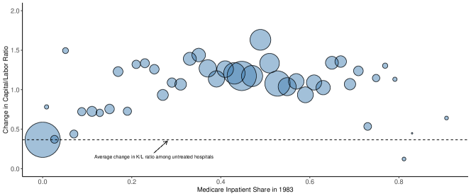
Figure 4: Changes in Capital-Labor Ratios before and after 1983 versus the Medicare Inpatient Share

Notes: The figure presents a binned scatter plot of the change in the average depreciation share (capital-labor ratio) between the periods 1980-1983 and 1984-1986 for hospitals in 2-percentage-point bins of the 1983 Medicare inpatient share, $M$. In the lowest bin, hospitals with $M=0$ are plotted separately from hospitals with $M\in(0,0.02]$. We also consider a single bin for all hospitals with $M>0.84$.

The horizontal line equals the mean change in capital-labor ratio for untreated hospitals (0.37), each circle is the mean outcome change for a given bin of the Medicare inpatient share, with their size proportional to the number of hospitals in that bin. Almost all groups of treated hospitals had stronger growth in capital intensity than untreated hospitals, consistent with the theoretical prediction. The relationship is nonlinear, however, which indicates heterogeneity in average treatment effects, at least, and perhaps heterogeneity in the sign of average causal responses.

6.2 Average Treatment Effects of PPS

Figure 5 presents our proposed data-adaptive nonparametric estimates of $ATT(m|m)$ based on Equation (4.9), formalizing what the scatter plot suggests: that $ATT(m|m)$ is positive. We plot pointwise 95% confidence intervals in the dark-shaded region and the wider uniform 95% confidence bands in the light-shaded region. We do not detect an effect for values of $m$ below 5 percent, but we reject zero for doses between 0.05 and 0.78, which contains 96 percent of treated hospitals. Significant values of $\widehat{ATT}(m|m)$ range from about 0.44 percentage points at $m=0.1$ and 0.88 percentage points at $m=0.41$. The average across all doses ($ATT^{o}$) is 0.80 (s.e. = 0.05), or about 18 percent of the 1983 mean outcome (measured by the depreciation share) of 4.5. This evidence suggests that PPS substantially raised capital-labor ratios.

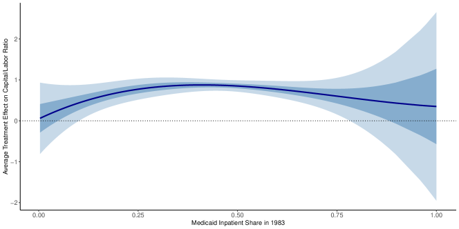
Figure 5: Nonparametric Estimates of $ATT(m|m)$ for Medicare PPS

Notes: The figure plots nonparametric estimate of $ATT(m|m)$ using the methods proposed in Section 4.1. The dark-shaded region is the 95-percent point-wise confidence interval, and the lighter-shaded region is the 95-percent uniform confidence band.

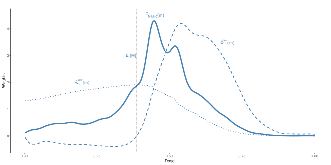
Figure 6: Weighting Schemes for TWFE and Dose Distribution Among Treated

Notes: The dashed lines are the weights that TWFE puts on $ATT(m|m)$ and $ACR(m)$ parameters, as in Theorem 3.4. The solid line is a smoothed estimate of the density of the Medicare inpatient share, $M$.

In Section 3.3, we argued that $\beta^{twfe}$ should not be relied upon to summarize level effects. However, the TWFE coefficient is 1.14—fairly similar to our estimate of $ATT^{o}$. What explains the difference? One explanation comes from Equation 3.1. The numerator compares weighted averages of the paths of outcomes for the “effective” treated group (those with above-average doses) to the “effective” comparison group (those with below-average doses). However, in our example, slightly more than half of the weight on paths of outcomes in the effective comparison group falls on hospitals with a positive dose. That these treated hospitals show up in the effective comparison group biases $\beta^{twfe}$ downward relative to $ATT^{o}$—our estimate of the numerator in Equation 3.1 is 0.60. In contrast, the “weighted distance” between the effective treated and comparison groups in the denominator of Equation 3.1 is estimated to be 0.53—that this is less than 1 is a byproduct of our setting where we measure a hospital’s dose on a scale of 0 to 1. Dividing by 0.53 results in our estimate of $\beta^{twfe}$ being upward biased. That these two biases work in opposite directions and have similar magnitudes in our particular application result in $\widehat{\beta}^{twfe}$ being fairly close to $\widehat{ATT}^{o}$.

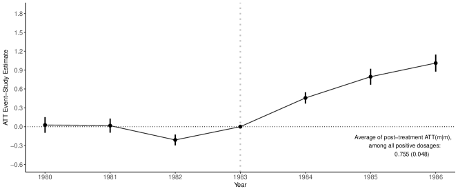
Figure 7: Event-Study Estimates of $ATT$

Notes: The figure plots the event-study estimates of $ATT^{es}(e)$ and their 95% confidence intervals.

Figure 5 abstracts from dynamics since it is based on average outcomes in the pre- and post-treatment periods. As an alternative, Figure 7 plots estimates of event-study summary parameters, $ATT^{es}(e)=\mathbb{E}[Y_{t=e}-Y_{t=1983}|D>0]-\mathbb{E}[Y_{t=e}-Y_{t=1983}|D=0]$, using 1983 as the baseline year. The patterns are similar to the TWFE event-study in Figure 1, but their magnitudes reflect proper averages of year-specific $ATT(m|m)$ parameters.

6.3 Average Causal Responses to PPS

Figure 8 plots our proposed data-adaptive nonparametric estimate of the slope of the function estimated in Figure 5. Under strong parallel trends as in Assumption 5, the function in Figure 5 is the $ATE(m)$ and its slope in Figure 8 equals the $ACR(m)$. The hump shape in Figure 5 is reflected in an $ACR(m)$ function that starts positive, and declines through most of its support. We estimate negative $ACR(m)$ parameters for doses above $m=0.41$, a range that includes 71 percent of treated hospitals. The 95% uniform confidence interval covers zero everywhere, although we are able to detect positive $ACR(m)$ values for doses below the mean as well negative $ACR(m)$ values for doses between about 0.5 and 0.7 using pointwise confidence intervals.

PPS’ average causal response parameter weighted by the actual dose distribution of treated hospitals is $\widehat{ACR}^{o}=-0.08$ (s.e. = 0.19) and is not significantly different from zero. This differs substantially from the TWFE coefficient, $\widehat{\beta}^{twfe}=1.14$. From Theorem 3.4, the difference between these estimates is fully driven by differences in the weighting scheme. Our estimate of $ACR^{o}$ comes from mapping the estimates of $ACR(m)$ in Figure 8 to the dose distribution weights, $\widehat{f}_{M|M>0}(m)$, in Figure 6; our estimate of $\beta^{twfe}$ comes from mapping the estimates of $ACR(m)$ to the TWFE causal response weights, $\widehat{w}_{1}^{acr}(m)$, in Figure 6. As discussed in Theorem 3.4, the TWFE causal response weights are positive for all values of the dose and integrate to one, providing a reason to hope that estimates of $ACR^{o}$ and $\beta^{twfe}$ would be similar. However, the TWFE weighting scheme turns out to be much different from the dose distribution weighting scheme. Combining these differences with the high degree of heterogeneity in $ACR(m)$ across $m$ is what leads to the sharp differences in the estimates. Another reason to emphasize the large difference between these estimates is that the literature has often viewed negative weights as a dividing line between an “unreasonable” or “reasonable” weighting scheme (see, e.g., [5, 26, 12] for related discussions of this point in different contexts). The results here suggest that, at least in our context, articulating a well-defined causal effect parameter and targeting that parameter directly is likely to be more important than checking that weights are all positive and integrate to one.

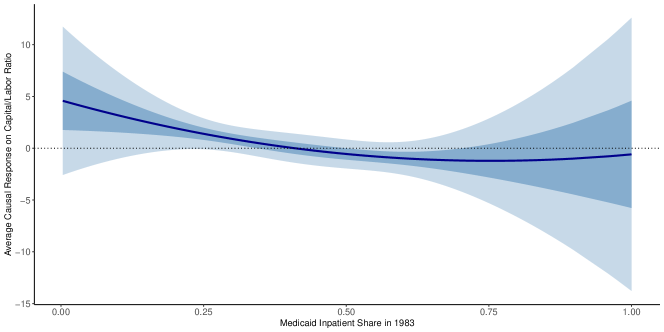
Figure 8: Nonparametric Estimates of $ACR(m)$ for Medicare PPS

Notes: The figure plots nonparametric estimate of $ACR(m)$ using the methods proposed in Section 4.1.

One major policy implication of these estimates is that Medicare could have achieved similar, if not greater capital investments while providing lower capital subsidies. Figure 8 shows that marginal increments in the subsidy ratio increase capital intensity only for those with low subsidy levels. The strong parallel trends assumption means that these estimated responses are externally valid for all hospitals. Under that assumption, the results imply that only low subsidies matter for hospitals’ input choices. Because higher subsidy ratios do not create further investments in capital, capping capital subsidies may not affect input choices very much.

Unlike the positive treatment effect parameters in Figure 5, however, the fact that $ACR(m)$ is negative at most dose values contradicts the predictions from AF’s economic model. $ACR(m)$ is proportional to the average derivative of the optimal capital-labor ratio for hospitals with Medicare share equal to $m$, and (6.1) shows specifically how it relates to the elasticity of substitution, $\sigma_{i,t}(m)$. To approximate $\mathbb{E}[\sigma_{i,t=2}(m)]$, we separate out the two terms in (6.1) and construct $\frac{ACR(m)}{\mathbb{E}[Y_{i,{t=2}}|M=m]}\frac{1-s_{k}m}{s_{k}}$ assuming that $s_{k}=0.75$. With only two inputs, a rise in the relative price of one must lead to a reduction in its relative use: the elasticity of substitution must be positive. The point estimates of $\mathbb{E}[\sigma_{i,t=2}(m)]$ do not fit that prediction although our uniform confidence bands do not reject an average elasticity of substitution of zero. Hospitals with the smallest Medicare shares have very high elasticity estimates; greater than two. This declines quickly, however, and is small and negative everywhere that $ACR(m)<0$. Some hospitals that received larger capital subsidies under PPS responded to it with smaller increases in capital intensity than hospitals with slightly smaller subsidies, a fact easily seen in the binned scatter plot in Figure 4.

Finally, both the policy and structural interpretations of Figure 8 require the strong parallel trends assumption. Without SPT, the slope of $ATT(m|m)$ may be negative for higher-Medicare-share hospitals simply because their treatment effect functions are systematically lower. Medicare might not have been able to achieve similar capital increases with lower subsidy rates if high-subsidy hospitals responded differently to low subsidy levels than low-subsidy hospitals did. It also does not necessarily negate the neoclassical theoretical prediction of a positive elasticity of substitution.

One way to assess the plausibility of SPT that justifies a causal interpretation of $ACR^{o}$ is to compute $ACR^{es}(e)$, the event-study version of $ACR^{o}$. These parameters can be estimated using the same procedure discussed in Section 4, and we plot these in Figure 9. As one can see, we detect sizable violations of SPT in 1981, which is a pre-treatment period. Interpreting that violations of strong parallel pre-trends as informative as violations of SPT in post-treatment periods, Figure 9 corroborates our conclusions about the implausibility of SPT based on implausibly high implied elasticities of substitution.

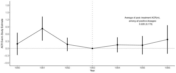
Figure 9: Event-Study Estimates of $ACR$

Notes: The figure plots the event-study estimates of $ACR^{es}(e)$ and their 95% confidence intervals following a procedure analogous to those discussed in Section 4.

In summary, our empirical results align with AF’s conclusion that the 1983 Medicare reform led hospitals to favor capital over labor. We find evidence against parallel trends in pre-treatment periods, though the magnitudes of these violations are small relative to estimated effects in post-treatment periods. Finally, our negative estimates of $ACR(m)$ at high values of $m$ cut against the theoretical predictions of the model discussed above; this provides a piece of evidence against strong parallel trends (and, hence, parameters/interpretations that rely on strong parallel trends) in this application.

Appendix A Additional Assumptions

Let $\Delta Y-\mathbb{E}[\Delta Y|D=0]=h(D)+u$. Under Assumption 4, $h(d)=ATT(d|d)$, whereas under Assumption 5, $h(d)=ATE(d)$. Let $\overline{\sigma},\underline{\sigma},\overline{C},\underline{c}$ be some finite, positive constants, and $\rho\in(0,1)$. Finally, let

$$\sigma^{2}_{K}(d)=\psi^{K}(d)^{\prime}\mathbb{E}\left[\left.\psi^{K}(D)\psi^{K}(D)^{\prime}\right|D>0\right]^{-}\mathbb{E}\left[\left.u^{2}\psi^{K}(D)\psi^{K}(D)^{\prime}\right|D>0\right]\mathbb{E}\left[\left.\psi^{K}(D)\psi^{K}(D)^{\prime}\right|D>0\right]^{-}\psi^{K}(d),$$

and $\left|\left|\sigma_{d,K}\right|\right|^{2}=\psi^{K}(d)^{\prime}\mathbb{E}\left[\left.\psi^{K}(D)\psi^{K}(D)^{\prime}\right|D>0\right]^{-}\psi^{K}(d)$, which satisfies $\left|\left|\sigma_{d,K}\right|\right|\asymp\sigma_{K}(d)$ under Assumption 6(i) below. Let $\left|\left|\sigma_{d,K}^{acr}\right|\right|^{2}=(\partial\psi^{K}(d))^{\prime}\mathbb{E}\left[\left.\psi^{K}(D)\psi^{K}(D)^{\prime}\right|D>0\right]^{-}(\partial\psi^{K}(d))$.

Assumption 6 (Additional regularity conditions).

a

1. $\mathbb{P}\left(\mathbb{E}\left[u^{4}|D,D>0\right]\leq\overline{\sigma}^{2}\right)=1$, and $\mathbb{P}\left(\mathbb{E}\left[u^{2}|D,D>0\right]\geq\underline{\sigma}^{2}\right)=1$.

2. $\underline{c}K\leq\inf_{d\in\mathcal{D}_{+}^{c}}\left|\left|\sigma_{d,K}\right|\right|^{2}\leq\sup_{d\in\mathcal{D}_{+}^{c}}\left|\left|\sigma_{d,K}\right|\right|^{2}\leq\overline{C}K$ for all $K\in\mathcal{K}$;

3. $\limsup_{K\rightarrow\infty}\sup_{d\in\mathcal{D}_{+}^{c},K_{2}\in\mathcal{K}:K_{2}>K}(\sigma_{K}^{2}(d)\big{/}\sigma_{K_{2}}^{2}(d))<\rho$;

4. $\underline{c}K^{3}\leq\inf_{d\in\mathcal{D}_{+}^{c}}\left|\left|\sigma_{d,K}^{acr}\right|\right|^{2}\leq\sup_{d\in\mathcal{D}_{+}^{c}}\left|\left|\sigma_{d,K}^{acr}\right|\right|^{2}\leq\overline{C}K^{3}$ for all $K\in\mathcal{K}$.

Assumption 6(iv) is only needed for Theorem 4.2(b), but we keep this assumption here for simplicity.

The next assumption is only used to establish the large sample properties of our average derivative estimator.

Assumption 7 (Regularity conditions for average derivatives).

a

1. $f_{D|D>0}(d)$ is continuously differentiable and is zero in the boundary of $\mathcal{D}_{+}^{c}$.

2. $\mathbb{E}\left[\left(\dfrac{f^{\prime}_{D|D>0}(D)}{f_{D|D>0}(D)}\right)^{2}\bigg{|}D>0\right]<\infty$, where $f^{\prime}_{D|D>0}(d)=\dfrac{df_{D|D>0}(a)}{da}\bigg{|}_{a=d}$.

Assumption 7(a) should be understood as imposing slightly stronger conditions than 2(a), as it requires additional smoothness conditions on the density of the dosage. It also requires the density to go to zero in the boundary of the dose. When applied together with Assumption 2(a), Assumption 7(a) should be understood as ruling out positive density in the boundary of treatment dose. These conditions are similar to those discussed in Example 2.1 and Section 4.1 of [3].

Appendix B Proofs of Main Results

B.1 Proofs of Results in Section 3.2

This section contains the proofs of the results in Section 3.2 on identifying causal effect parameters such as $ATT(d|d)$ and $ATE(d)$ under parallel trends assumptions and with a continuous treatment or multi-valued discrete treatment.

Proof of Theorem 3.1

Proof.

To show the result, notice that

$$ATT(d|d) =\mathbb{E}[Y_{t=2}(d)-Y_{t=2}(0)|D=d]$$

$$=\mathbb{E}[Y_{t=2}(d)-Y_{t=1}(0)|D=d]-\mathbb{E}[Y_{t=2}(0)-Y_{t=1}(0)|D=d]$$

$$=\mathbb{E}[Y_{t=2}(d)-Y_{t=1}(0)|D=d]-\mathbb{E}[Y_{t=2}(0)-Y_{t=1}(0)|D=0]$$

$$=\mathbb{E}[\Delta Y|D=d]-\mathbb{E}[\Delta Y|D=0]$$ (B.1)

where the second equality holds by adding and subtracting $\mathbb{E}[Y_{t=1}(0)|D=d]$, the third equality holds by Assumption 4, and the last equality holds because $Y_{t=2}(d)$ and $Y_{t=1}(0)$ are observed potential outcomes when $D=d$ and $Y_{t=2}(0)$ and $Y_{t=1}(0)$ are observed potential outcomes when $D=0$. That $ATT^{o}$ is identified holds immediately given its definition and that $ATT(d|d)$ is identified. To derive the particular expression for $ATT^{o}$, notice that

$$ATT^{o} =\mathbb{E}\Big{[}ATT(D|D)\Big{|}D>0\Big{]}$$

$$=\mathbb{E}\Big{[}\Big{(}\mathbb{E}[\Delta Y|D]-\mathbb{E}[\Delta Y|D=0]\Big{)}\Big{|}D>0\Big{]}$$

$$=\mathbb{E}[\Delta Y|D>0]-\mathbb{E}[\Delta Y|D=0]$$

where the first equality is the definition of $ATT^{o}$, the second equality holds from Equation B.1, the first part of the third equality holds by an implication of the law of iterated expectations, and the second part of the third equality holds because $\mathbb{E}[\Delta Y|D=0]$ is non-random. ∎

Proof of Theorem 3.2

Proof.

We start by proving the first result in part (b). Notice that

$$\mathbb{E}[\Delta Y|D=h]-\mathbb{E}[\Delta Y|D=l] =\Big{(}\mathbb{E}[\Delta Y|D=h]-\mathbb{E}[\Delta Y|D=0]\Big{)}-\Big{(}\mathbb{E}[\Delta Y|D=l]-\mathbb{E}[\Delta Y|D=0]\Big{)}$$

$$=ATT(h|h)-ATT(l|l)$$ (B.2)

where the first equality holds by adding and subtracting $\mathbb{E}[\Delta Y|D=0]$, and the second equality holds by Theorem 3.1. Next,

$$ATT(h|h)-ATT(l|l) =\mathbb{E}[Y_{t=2}(h)-Y_{t=2}(0)|D=h]-\mathbb{E}[Y_{t=2}(l)-Y_{t=2}(0)|D=l]$$

$$=\mathbb{E}[Y_{t=2}(h)-Y_{t=2}(l)|D=h]$$

$$~{}~{}~{}+\mathbb{E}[Y_{t=2}(l)-Y_{t=2}(0)|D=h]-\mathbb{E}[Y_{t=2}(l)-Y_{t=2}(0)|D=l]$$

$$=\mathbb{E}[Y_{t=2}(h)-Y_{t=2}(l)|D=h]+\Big{(}ATT(l|h)-ATT(l|l)\Big{)}$$ (B.3)

where the first equality holds by the definition of $ATT(d|d)$, the second equality holds by adding and subtracting $\mathbb{E}[Y_{t=2}(l)|D=h]$, and the third equality holds by the definition of $ATT(l|h)$ and $ATT(l|l)$. Notice that $\mathbb{E}[Y_{t=2}(h)-Y_{t=2}(l)|D=h]$ is a causal response of going from dose $l$ to dose $h$ for dose group $h$. An alternative expression for this term is

$$\mathbb{E}[Y_{t=2}(h)-Y_{t=2}(l)|D=h]=ATT(h|h)-ATT(l|h)$$ (B.4)

Next, we prove part (a). Using a similar argument as above, notice that, for $d\in\mathcal{D}_{+}^{c}$ and $(d+h)\in\mathcal{D}_{+}^{c}$,

$$\frac{\mathbb{E}[\Delta Y|D=d]-\mathbb{E}[\Delta Y|D=d+h]}{h} =\frac{ATT(d|d)-ATT(d+h|d+h)}{h}$$

$$=\frac{ATT(d|d)-ATT(d+h|d)}{h}+\frac{ATT(d+h|d)-ATT(d+h|d+h)}{h}$$

where the first equality holds using the same argument as for Equation B.2, and the second equality holds by using the arguments in Equations B.3 and B.4. The result holds by taking the limit as $h\rightarrow 0$ and the definition of $ACRT(d|d)$.

Finally, the second result in part (b) involving a discrete treatment holds by taking $h=d_{j}$ and $l=d_{j-1}$ in Equations B.2 and B.3 and by the definition of $ACRT(d_{j}|d_{j})$. ∎

Proof of Theorem 3.3

Proof.

For part (a), notice that

$$ATE(d) =\mathbb{E}[Y_{t=2}(d)-Y_{t=2}(0)]$$

$$=\mathbb{E}[Y_{t=2}(d)-Y_{t=1}(0)]-\mathbb{E}[Y_{t=2}(0)-Y_{t=1}(0)]$$

$$=\mathbb{E}[Y_{t=2}(d)-Y_{t=1}(0)|D=d]-\mathbb{E}[Y_{t=2}(0)-Y_{t=1}(0)|D=0]$$

$$=\mathbb{E}[\Delta Y|D=d]-\mathbb{E}[\Delta Y|D=0]$$

where the second equality holds by adding and subtracting $\mathbb{E}[Y_{t=1}(0)]$, the third equality holds by Assumption 5, and the fourth equality holds because $Y_{t=2}(d)$ and $Y_{t=1}(0)$ are observed outcomes when $D=d$.

Next, we prove the first part of part (c). First, notice that

$$ATE(h)-ATE(l)=\mathbb{E}[Y_{t=2}(h)-Y_{t=2}(0)]-\mathbb{E}[Y_{t=2}(l)-Y_{t=2}(0)]=\mathbb{E}[Y_{t=2}(h)-Y_{t=2}(l)]$$

where the first equality holds by the definition of $ATE(d)$, and the second equality holds by cancelling the terms involving $Y_{t=2}(0)$. Next, notice that

$$ATE(h)-ATE(l) =\Big{(}\mathbb{E}[\Delta Y|D=h]-\mathbb{E}[\Delta Y|D=0]\Big{)}-\Big{(}\mathbb{E}[\Delta Y|D=l]-\mathbb{E}[\Delta Y|D=0]\Big{)}$$

$$=\mathbb{E}[\Delta Y|D=h]-\mathbb{E}[\Delta Y|D=l]$$

Now, for part (b), notice that for $d\in\mathcal{D}_{+}^{c}$ and $(d+h)\in\mathcal{D}_{+}^{c}$,

$$\frac{ATE(d)-ATE(d+h)}{h}=\frac{\mathbb{E}[\Delta Y|D=d]-\mathbb{E}[\Delta Y|D=d+h]}{h}$$

which follows from part (a). The result holds by taking the limit as $h\rightarrow 0$ and from the definition of $ACR(d)$.

Finally, the result in part (c) involving a discrete treatment holds from part (a) by taking $h=d_{j}$ and $l=d_{j-1}$. ∎

Proof of Corollary 3.1

Proof.

The result holds immediately by averaging the results in Theorem 3.1 over the distribution of the dose among dose groups that experienced any positive amount of the treatment. ∎

B.2 Proofs of Results from Section 3.3

This section contains the proofs of the results in Theorem 3.4 in Section 3.3 on interpreting TWFE regressions with a continuous treatment. To conserve on notation, we define

$$m_{\Delta}(d)=\mathbb{E}[\Delta Y|D=d],$$

We divide the proofs according to each part of the theorem. In the proof, we derive all the results in terms of $m_{\Delta}(d)$. This results in a mechanical decomposition in the sense that $\widehat{\beta}^{twfe}$ is equal to the sample analog of each derived quantity below. The result in Theorem 3.4 is stated in terms of various causal building block parameters. Those results follow immediately from the ones below by noting that, under Assumption 4,

• $m_{\Delta}(d)-m_{\Delta}(0)=ATT(d|d)$

• $m^{\prime}_{\Delta}(d)=ACRT(d|d)+\underbrace{\frac{\partial ATT(d|h)}{\partial h}\Big{|}_{h=d}}_{\textrm{selection bias}}$

• $m_{\Delta}(h)-m_{\Delta}(l)=ATT(h|h)-ATT(l|l)=\mathbb{E}[Y_{t}(h)-Y_{t}(l)|D=h]+\underbrace{\Big{(}ATT(l|h)-ATT(l|l)\Big{)}}_{\textrm{selection bias}}$

or, when Assumption 5 holds,

• $m_{\Delta}(d)-m_{\Delta}(0)=ATE(d)$

• $m^{\prime}_{\Delta}(d)=ACR(d)$

• $m_{\Delta}(h)-m_{\Delta}(l)=ATE(h)-ATE(l)=\mathbb{E}[Y_{t=2}(h)-Y_{t=2}(l)]$

Proof of Theorem 3.4(a)

Proof.

First, notice that Equation 1.1 is equivalent to

$$\Delta Y_{i}=(\theta_{t=2}-\theta_{t=1})+\beta^{twfe}D_{i}+\Delta v_{i,t}$$ (B.5)

which holds by taking first differences and because all units are untreated in the first period. Therefore, it immediately follows that

$$\beta^{twfe} =\frac{\mathbb{E}[\Delta Y(D-\mathbb{E}[D])]}{\mathrm{Var}(D)}$$

$$=\mathbb{E}\left[\frac{(D-\mathbb{E}[D])}{\mathrm{Var}(D)}(m_{\Delta}(D)-m_{\Delta}(0))\right]$$

$$=\mathbb{E}\left[\frac{(D-\mathbb{E}[D])}{\mathrm{Var}(D)}(m_{\Delta}(D)-m_{\Delta}(0))\Big{|}D>0\right]\mathbb{P}(D>0)$$

$$=\mathbb{E}\left[\frac{(D-\mathbb{E}[D])}{\mathrm{Var}(D)}(m_{\Delta}(D)-m_{\Delta}(d_{L}))\Big{|}D>0\right]\mathbb{P}(D>0)$$

$$+\mathbb{E}\left[\frac{(D-\mathbb{E}[D])}{\mathrm{Var}(D)}(m_{\Delta}(d_{L})-m_{\Delta}(0))\Big{|}D>0\right]\mathbb{P}(D>0)$$ (B.6)

$$=A_{1}+A_{2}$$

where the first equality holds because Equation B.5 is a simple linear regression of $\Delta Y$ on an intercept and $D$, the second equality holds by the law of iterated expectations and because $\mathbb{E}[(D-\mathbb{E}[D])m_{\Delta}(0)]=0$, the third equality holds because $\mathbb{E}[m_{\Delta}(D)-m_{\Delta}(0)|D=0]=0$, and the fourth equality holds by adding and subtracting $m_{\Delta}(d_{L})$ inside the expectation.

We consider $A_{1}$ and $A_{2}$ separately next. First, for $A_{1}$,

$$A_{1} =\mathbb{E}\left[\frac{(D-\mathbb{E}[D])}{\mathrm{Var}(D)}(m_{\Delta}(D)-m_{\Delta}(d_{L}))\Big{|}D>0\right]\mathbb{P}(D>0)$$

$$=\frac{\mathbb{P}(D>0)}{\mathrm{Var}(D)}\int_{d_{L}}^{d_{U}}(k-\mathbb{E}[D])(m_{\Delta}(k)-m_{\Delta}(d_{L}))\,dF_{D|D>0}(k)$$

$$=\frac{\mathbb{P}(D>0)}{\mathrm{Var}(D)}\int_{d_{L}}^{d_{U}}(k-\mathbb{E}[D])\int_{d_{L}}^{k}m^{\prime}_{\Delta}(l)\,dl\,dF_{D|D>0}(k)$$

$$=\frac{\mathbb{P}(D>0)}{\mathrm{Var}(D)}\int_{d_{L}}^{d_{U}}(k-\mathbb{E}[D])\int_{d_{L}}^{d_{U}}\mathbf{1}\{l\leq k\}m^{\prime}_{\Delta}(l)\,dl\,dF_{D|D>0}(k)$$

$$=\frac{\mathbb{P}(D>0)}{\mathrm{Var}(D)}\int_{d_{L}}^{d_{U}}m^{\prime}_{\Delta}(l)\int_{d_{L}}^{d_{U}}(k-\mathbb{E}[D])\mathbf{1}\{l\leq k\}\,dF_{D|D>0}(k)\,dl$$

$$=\frac{\mathbb{P}(D>0)}{\mathrm{Var}(D)}\int_{d_{L}}^{d_{U}}m^{\prime}_{\Delta}(l)\mathbb{E}[(D-\mathbb{E}[D])\mathbf{1}\{l\leq D\}|D>0]\,dl$$

$$=\frac{\mathbb{P}(D>0)}{\mathrm{Var}(D)}\int_{d_{L}}^{d_{U}}m^{\prime}_{\Delta}(l)\mathbb{E}[(D-\mathbb{E}[D])|D\geq l]\mathbb{P}(D\geq l|D>0)\,dl$$

$$=\int_{d_{L}}^{d_{U}}m^{\prime}_{\Delta}(l)\frac{(\mathbb{E}[D|D\geq l]-\mathbb{E}[D])\mathbb{P}(D\geq l)}{\mathrm{Var}(D)}\,dl$$ (B.7)

where the first equality is the definition of $A_{1}$, the second equality holds by rearranging terms and writing the expectation as an integral, the third equality holds by the fundamental theorem of calculus, the fourth equality rewrites the inner integral so that it is over $d_{L}$ to $d_{U}$, the fifth equality holds by changing the order of integration and rearranging terms, the sixth equality holds by rewriting the inner integral as an expectation, the seventh equality holds by the law of iterated expectations (and since $D\geq l\implies D>0$), and the last equality holds by combining terms.

Next, for $A_{2}$, it immediately holds that

$$A_{2} =\mathbb{E}\left[\frac{(D-\mathbb{E}[D])}{\mathrm{Var}(D)}(m_{\Delta}(d_{L})-m_{\Delta}(0))\Big{|}D>0\right]\mathbb{P}(D>0)$$

$$=\frac{(\mathbb{E}[D|D>0]-\mathbb{E}[D])\mathbb{P}(D>0)d_{L}}{\mathrm{Var}(D)}\frac{(m_{\Delta}(d_{L})-m_{\Delta}(0))}{d_{L}}$$ (B.8)

where the first equality is the definition of $A_{2}$, and the second equality holds by multiplying and dividing by $d_{L}$.

Then, the first result in Part (a) holds by combining Equations B.7 and B.8. That the weights are all positive holds immediately since $(\mathbb{E}[D|D\geq l]-\mathbb{E}[D])>0$ for all $l\geq d_{L}$, $\mathbb{P}(D\geq l)>0$ for all $l\geq d_{L}$, $(\mathbb{E}[D|D>0]-\mathbb{E}[D])>0$, $\mathbb{P}(D>0)>0$, and $\mathrm{Var}(D)>0$.

Next, we next show that $\int_{d_{L}}^{d_{U}}w_{1}^{acr}(l)\,dl+w_{0}^{acr}=1$. First, notice that

$$\int_{d_{L}}^{d_{U}}w_{1}^{acr}(l)\,dl+w_{0}^{acr} =\frac{1}{\mathrm{Var}(D)}\Bigg{\{}\int_{d_{L}}^{d_{U}}\mathbb{E}[D|D\geq l]\mathbb{P}(D\geq l)\,dl$$

$$\hskip 50.0pt-\mathbb{E}[D]\int_{d_{L}}^{d_{U}}\mathbb{P}(D\geq l)\,dl$$

$$\hskip 50.0pt+\mathbb{E}[D|D>0]\mathbb{P}(D>0)d_{L}$$

$$\hskip 50.0pt-\mathbb{E}[D]\mathbb{P}(D>0)d_{L}\Bigg{\}}$$

$$=\frac{1}{\mathrm{Var}(D)}\Big{\{}B_{1}-B_{2}+B_{3}-B_{4}\Big{\}}$$

and we consider $B_{1},B_{2},B_{3}$, and $B_{4}$ in turn.

For $B_{1}$, first notice that for all $l\in\mathcal{D}_{+}^{c}$,

$$\mathbb{E}[D|D\geq l]\mathbb{P}(D\geq l) =\mathbb{E}[D\mathbf{1}\{D\geq l\}|D\geq l]\mathbb{P}(D\geq l)$$

$$=\mathbb{E}[D\mathbf{1}\{D\geq l\}]$$ (B.9)

which holds by the law of iterated expectations and implies that

$$B_{1} =\int_{d_{L}}^{d_{U}}\mathbb{E}[D|D\geq l]\mathbb{P}(D\geq l)\,dl$$

$$=\int_{d_{L}}^{d_{U}}\int_{\mathcal{D}}d\mathbf{1}\{d\geq l\}\,dF_{D}(d)\,dl$$

$$=\int_{\mathcal{D}}d\left(\int_{d_{L}}^{d_{U}}\mathbf{1}\{l\leq d\}\,dl\right)\,dF_{D}(d)$$

$$=\int_{\mathcal{D}}d(d-d_{L})\,dF_{D}(d)$$

$$=\mathbb{E}[D^{2}]-\mathbb{E}[D]d_{L}$$ (B.10)

where the first line is the definition of $B_{1}$, the second equality holds by Equation B.9, the third equality holds by changing the order of integration, the fourth equality holds by carrying out the inner integration, and the last equality holds by rewriting the integral as an expectation.

Next, for term $B_{2}$,

$$B_{2} =\mathbb{E}[D]\int_{d_{L}}^{d_{U}}\mathbb{P}(D\geq l)\,dl$$

$$=\mathbb{E}[D]\mathbb{P}(D>0)\int_{d_{L}}^{d_{U}}\mathbb{P}(D\geq l|D>0)\,dl$$

$$=\mathbb{E}[D]\mathbb{P}(D>0)\int_{d_{L}}^{d_{U}}\int_{d_{L}}^{d_{U}}\mathbf{1}\{d\geq l\}\,dF_{D|D>0}(d)\,dl$$

$$=\mathbb{E}[D]\mathbb{P}(D>0)\int_{d_{L}}^{d_{U}}\left(\int_{d_{L}}^{d_{U}}\mathbf{1}\{l\leq d\}\,dl\right)\,dF_{D|D>0}(d)$$

$$=\mathbb{E}[D]\mathbb{P}(D>0)\int_{d_{L}}^{d_{U}}(d-d_{L})\,dF_{D|D>0}(d)$$

$$=\mathbb{E}[D]\mathbb{P}(D>0)\Big{(}\mathbb{E}[D|D>0]-d_{L}\Big{)}$$

$$=\mathbb{E}[D]^{2}-\mathbb{E}[D]\mathbb{P}(D>0)d_{L}$$ (B.11)

where the first equality is the definition of $B_{2}$, the second equality holds by the law of iterated expectations, the third equality holds by writing $\mathbb{P}(D\geq l|D>0)$ as an integral, the fourth equality changes the order of integration, the fifth equality carries out the inside integration, the sixth equality rewrites the integral as an expectation, and the last equality holds by combining terms and by the law of iterated expectations.

Next,

$$B_{3} =\mathbb{E}[D|D>0]\mathbb{P}(D>0)d_{L}$$

$$=\mathbb{E}[D]d_{L}$$ (B.12)

which holds by the law of iterated expectations. And finally, recall that

$$B_{4}=\mathbb{E}[D]\mathbb{P}(D>0)d_{L}$$ (B.13)

Thus, from Equations B.10, B.11, B.12 and B.13, it follows that

$$B_{1}-B_{2}+B_{3}-B_{4}=\mathbb{E}[D^{2}]-\mathbb{E}[D]^{2}=\mathrm{Var}(D)$$

which implies the result.

∎

Proof of Theorem 3.4(b)

Proof.

From the proof of Part (a), we have that

$$\beta^{twfe} =\frac{\mathbb{P}(D>0)}{\mathrm{Var}(D)}\mathbb{E}\left[(D-\mathbb{E}[D])(m_{\Delta}(D)-m_{\Delta}(0))\Big{|}D>0\right]$$

$$=\frac{\mathbb{P}(D>0)}{\mathrm{Var}(D)}\int_{d_{L}}^{d_{U}}(l-\mathbb{E}[D])(m_{\Delta}(l)-m_{\Delta}(0))\,dF_{D|D>0}(l)$$

$$=\frac{1}{\mathrm{Var}(D)}\int_{d_{L}}^{d_{U}}(l-\mathbb{E}[D])(m_{\Delta}(l)-m_{\Delta}(0))f_{D}(l)\,dl$$

$$=\int_{d_{L}}^{d_{U}}w_{1}^{lev}(l)(m_{\Delta}(l)-m_{\Delta}(0))\,dl$$

where the second equality holds by writing the expectation as an integral, the third equality holds under Assumption 2(a), and the last equality holds by the definition of $w_{1}^{lev}$.

Next, we show the properties of the weights for this part of the theorem. The weights can be negative since $l$ can be less than $\mathbb{E}[D]$. To see that the weights integrate to zero, first note that that $w_{0}^{lev}(m_{\Delta}(0)-m_{\Delta}(0))=0$, so that the previous expression for $\beta^{twfe}$ can equivalently be written as

$$\beta^{twfe}=\int_{d_{L}}^{d_{U}}w_{1}^{lev}(l)(m_{\Delta}(l)-m_{\Delta}(0))\,dl+w_{0}^{lev}(m_{\Delta}(0)-m_{\Delta}(0))$$

Then, notice that

$$\int_{d_{L}}^{d_{U}}w_{1}^{lev}(l)\,dl+w_{0}^{lev} =\left(\int_{d_{L}}^{d_{U}}(l-\mathbb{E}[D])\,dF_{D}(l)+(0-\mathbb{E}[D])\mathbb{P}(D=0)\right)\Big{/}\mathrm{Var}(D)$$

$$=\left(\int_{\mathcal{D}}(l-\mathbb{E}[D])\,dF_{D}(l)\right)\Big{/}\mathrm{Var}(D)$$

$$=(\mathbb{E}[D]-\mathbb{E}[D])/\mathrm{Var}(D)$$

$$=0$$

where the first equality holds by the definitions of $w_{1}^{lev}$ and $w_{0}^{lev}$, the second equality combines terms, and the third and fourth equalities hold immediately. This completes the proof. ∎

Proof of Theorem 3.4(c)

Proof.

From the proof of Theorem 3.4(a), we have that

$$\beta^{twfe} =\frac{\mathbb{P}(D>0)}{\mathrm{Var}(D)}\mathbb{E}\left[(D-\mathbb{E}[D])(m_{\Delta}(D)-m_{\Delta}(0))\Big{|}D>0\right]$$

$$=\frac{\mathbb{P}(D>0)}{\mathrm{Var}(D)}\int_{d_{L}}^{d_{U}}(l-\mathbb{E}[D])(m_{\Delta}(l)-m_{\Delta}(0))\,dF_{D|D>0}(l)$$

$$=\frac{\mathbb{P}(D>0)}{\mathrm{Var}(D)}\int_{d_{L}}^{d_{U}}(l-\mathbb{E}[D])l\frac{(m_{\Delta}(l)-m_{\Delta}(0))}{l}\,dF_{D|D>0}(l)$$

$$=\frac{1}{\mathrm{Var}(D)}\int_{d_{L}}^{d_{U}}(l-\mathbb{E}[D])l\frac{(m_{\Delta}(l)-m_{\Delta}(0))}{l}f_{D}(l)\,dl$$

$$=\int_{d_{L}}^{d_{U}}w^{s}(l)\frac{(m_{\Delta}(l)-m_{\Delta}(0))}{l}\,dl$$

where the second equality holds by writing the expectation as an integral, the third equality holds by multiplying and dividing by $l$, the fourth equality holds under Assumption 2(a), and the last equality holds by the definition of $w^{s}$.

The weights can be negative because it is possible that $l<\mathbb{E}[D]$ for some values of $l\in\mathcal{D}_{+}^{c}$. That the weights integrate to 1 holds because

$$\int_{d_{L}}^{d_{U}}w^{s}(l)\,dl =\left(\int_{d_{L}}^{d_{U}}(l-\mathbb{E}[D])l\,dF_{D}(l)+(0-\mathbb{E}[D])\,0\,\mathbb{P}(D=0)\right)\Big{/}\mathrm{Var}(D)$$

$$=\left(\int_{\mathcal{D}}(l-\mathbb{E}[D])l\,dF_{D}(l)\right)\Big{/}\mathrm{Var}(D)$$

$$=(\mathbb{E}[D^{2}]-\mathbb{E}[D]^{2})\Big{/}\mathrm{Var}(D)=1$$

where the first equality uses the definition of the weights and that $(0-\mathbb{E}[D])\,0\,\mathbb{P}(D=0)=0$, the second equality comes from combining terms, and the last line holds immediately. ∎

Proof of Theorem 3.4(d)

Proof.

From the proof of part (a), we have that

$$\beta =\mathbb{E}\left[\frac{(D-\mathbb{E}[D])}{\mathrm{Var}(D)}m_{\Delta}(D)\right]$$

$$=\frac{1}{\mathrm{Var}(D)}\int_{\mathcal{D}}(h-\mathbb{E}[D])m_{\Delta}(h)\,dF_{D}(h)$$

$$=\frac{1}{\mathrm{Var}(D)}\int_{\mathcal{D}}\left(h-\int_{\mathcal{D}}l\,dF_{D}(l)\right)m_{\Delta}(h)\,dF_{D}(h)$$

$$=\frac{1}{\mathrm{Var}(D)}\int_{\mathcal{D}}\int_{\mathcal{D}}(h-l)m_{\Delta}(h)\,dF_{D}(h)\,dF_{D}(l)$$

$$=\frac{1}{\mathrm{Var}(D)}\int_{\mathcal{D}}\int_{\mathcal{D},h>l}(h-l)(m_{\Delta}(h)-m_{\Delta}(l))\,dF_{D}(h)\,dF_{D}(l)$$

$$=\frac{1}{\mathrm{Var}(D)}\int_{\mathcal{D}}\int_{\mathcal{D},h>l}(h-l)^{2}\frac{(m_{\Delta}(h)-m_{\Delta}(l))}{(h-l)}\,dF_{D}(h)\,dF_{D}(l)$$ (B.14)

where the second equality holds by writing the expectation as an integral, the third equality by writing $\mathbb{E}[D]$ as an integral, the fourth equality rearranges terms, the fifth equality holds because the integrations are symmetric, and the last equality holds by multiplying and dividing by $(h-l)$.

The above arguments hold if the treatment is continuous or discrete. Under Assumption 2(a),

Equation (B.14) $$=\frac{1}{\mathrm{Var}(D)}\int_{d_{L}}^{d_{U}}\int_{\mathcal{D},h>l}(h-l)^{2}\frac{(m_{\Delta}(h)-m_{\Delta}(l))}{(h-l)}f_{D}(h)f_{D}(l)\,dh\,dl$$

$$+\frac{1}{\mathrm{Var}(D)}\int_{d_{L}}^{d_{U}}h^{2}\frac{m_{\Delta}(h)-m_{\Delta}(0)}{h}f_{D}(h)\mathbb{P}(D=0)\,dh$$

which holds by splitting up the first integral in Equation B.14 by whether $l\in\mathcal{D}_{+}^{c}$ or $l=0$. Then, the first part of this results holds by the definition of $w_{1}^{2\times 2}$ and $w_{0}^{2\times 2}$.

That the weights are all positive holds immediately by their definitions. That the weights integrate to one holds because

$$\int_{d_{L}}^{d_{U}}\int_{\mathcal{D},h>l}w_{1}^{2\times 2,cont}(l,h)\,dh\,dl+\int_{d_{L}}^{d_{U}}w_{0}^{2\times 2,cont}(h)\,dh =\frac{1}{\mathrm{Var}(D)}\int_{\mathcal{D}}\int_{\mathcal{D}}\mathbf{1}\{h>l\}(h-l)^{2}\,dF_{D}(h)\,dF_{D}(l)$$

$$=\frac{1}{2}\int_{\mathcal{D}}\int_{\mathcal{D}}(h-l)^{2}\,dF_{D}(h)\,dF_{D}(l)\Bigg{/}\mathrm{Var}(D)$$

$$=1$$

where the first equality holds by combining the integrals and the definition of the weights (it amounts to re-writing the integrals as in Equation B.14), the second equality holds because $\int_{\mathcal{D}}\int_{\mathcal{D}}\mathbf{1}\{h>l\}(h-l)^{2}\,dF_{D}(h)\,dF_{D}(l)=\int_{\mathcal{D}}\int_{\mathcal{D}}\mathbf{1}\{h\leq l\}(h-l)^{2}\,dF_{D}(h)\,dF_{D}(l)$ (and these two terms add up to the expression on the next line), and the third equality holds because the double integral is equal to $2\mathrm{Var}(D)$. This completes the proof. ∎

B.3 Proofs of Results from Section 4

Proof of Theorem 4.1

Proof.

Assumptions 1, 2(a), 3 and 5 guarantee identification of $ATE(d)$ and $ACR(d)$ using a nonparametric regression. With that in hand, the proof of Theorem 4.1 follows by verifying the Assumptions 1 to 4 from CCK, and then relying on their Theorem 4.1(a) and Corollary 4.1(a). Assumption 1 of CCK is satisfied by our Assumption 2(a) and the fact that we are considering a setup with nonparametric regression. Assumption 2 of CCK is implied by Assumption 6(i). Assumption 3 of CCK is trivially satisfied in our nonparametric regression setup. Assumption 4 of CCK is implied by Assumption 6(ii)-(iv). Thus, part(i) from Theorem 4.1 follows from Theorem 4.1(a) of CCK, while part (ii) follows from Corollary 4.1(a). ∎

Proof of Theorem 4.2

Proof.

Since Assumptions 1 to 4 from CCK are implied by Assumptions 2(a), 3, 5, and 6, Theorem 4.2(a) follows from Theorem 4.2 of CCK, while Theorem 4.2(b) follows from their Theorem 4.4. ∎

Proof of Theorem 4.3

Proof.

From Example 2.1 and the results in Section 4.1 of [3], by taking their $h_{2}(W_{2})=0$ a.s., we have that

$$\sqrt{n_{D>0}}{\left(\widehat{ACR}^{o}-ACR^{o}\right)}\overset{d}{\rightarrow}\mathcal{N}(0,V_{ACR}),$$

as Assumptions 1, 2(a), 3, 5, 6 and 7 imply Condition 2.1.1 and 2.1.2 of [3], with $s=1$. That $V_{ACR}$ is the semiparametric efficient bound for average derivatives follows from Theorem 3.1 of [40]. Finally, $\widehat{\sigma}^{2}_{ACR^{o}}\overset{p}{\rightarrow}V_{ACR}$ follows directly from [39] and [2]. Thus, Theorem 4.3 follows from the continuous mapping theorem. ∎

Appendix C Comparing Alternative Parallel Trends Assumptions

In this section, we introduce two alternative parallel trends assumptions. The first is an aggregated version of the parallel trends assumption which is weaker than the parallel trends assumption in Assumption 4 and that is specifically geared toward recovering $ATT^{o}$. Second, we consider an alternative (and stronger) version of the strong parallel trends assumption. Then, we provide a result that delivers a full comparison of (i) aggregate parallel trends, (ii) parallel trends, (iii) strong parallel trends, (iv) the combination of parallel trends and strong parallel trends, (v) the alternative strong parallel trends assumption, and characterizes the exact conditions under which these assumptions are equivalent to restrictions on treatment effect heterogeneity.

Assumption 4-Agg (Aggregate Parallel Trends).

$$\mathbb{E}[Y_{t=2}(0)-Y_{t=1}(0)|D>0]=\mathbb{E}[Y_{t=2}(0)-Y_{t=1}(0)|D=0]$$

4-Agg, which we refer to as aggregate parallel trends below, says that the average path of untreated potential outcomes among those that experienced any positive dose is equal to the path of untreated potential outcomes for the untreated group. This assumption essentially amounts to binarizing the treatment and then assuming parallel trends on the basis of the new binary treatment.

Assumption 5-Alt (Alternative Strong Parallel Trends Assumption).

For all $d\in\mathcal{D}$ and $l\in\mathcal{D}$,

$$\mathbb{E}[Y_{t=2}(d)-Y_{t=1}(0)|D=l]=\mathbb{E}[Y_{t=2}(d)-Y_{t=1}(0)|D=d]$$

5-Alt, which we refer to as alternative strong parallel trends below, is a stronger, but related version of the strong parallel trends assumption in Assumption 5. Alternative strong parallel trends states that across all doses $d$, the path of potential outcomes $Y_{t=2}(d)-Y_{t=1}(0)$ is, on average, (i) the same across all dose groups, $l$, and (ii) is equal to the average path of outcomes for units that actually experienced dose $d$. Further, note that $\mathbb{E}[Y_{t=2}(d)-Y_{t=1}(0)|D=l]$ is not identified from the sampling process except in the case where $l=d$ (i.e., the left-hand side of the equation in 5-Alt is not identified from the sampling process, but the right-hand side is). In the following, we use parallel trends and strong parallel trends to refer to Assumption 4 and Assumption 5, respectively, and aggregate parallel trends and alternative strong parallel trends to refer to 4-Agg and 5-Alt, respectively.

Theorem C.1.

Under Assumptions 1, 2 and 3, the following results hold:

• Identified parameters under different parallel trends assumptions:

  • Aggregate parallel trends $\implies$ $ATT^{o}=\mathbb{E}[\Delta Y|D>0]-\mathbb{E}[\Delta Y|D=0]$;

  • Parallel trends $\implies$ $ATT(d|d)=\mathbb{E}[\Delta Y|D=d]-\mathbb{E}[\Delta Y|D=0]$;

  • Strong parallel trends $\implies ATE(d)=\mathbb{E}[\Delta Y|D=d]-\mathbb{E}[\Delta Y|D=0]$;

  • Parallel trends plus strong parallel trends $\implies ATT(d|d)=ATE(d)=\mathbb{E}[\Delta Y|D=d]-\mathbb{E}[\Delta Y|D=0]$;

  • Alternative strong parallel trends $\implies ATT(d|d^{\prime})=ATT(d|d)=ATE(d)=\mathbb{E}[\Delta Y|D=d]-\mathbb{E}[\Delta Y|D=0]$.

• Non-identified parameters under different parallel trends assumptions:

  • Aggregate parallel trends does not recover $ATT(d|d)$ or $ATE(d)$;

  • Parallel trends does not recover $ATE(d)$;

  • Strong parallel trends does not recover $ATT(d|d)$;

  • Together parallel trends and strong parallel trends do not recover $ATT(d|d^{\prime})$ for $d\neq d^{\prime}$.

• Strength of different parallel trends assumptions:

  • Aggregate parallel trends does not imply parallel trends or strong parallel trends;

  • Either parallel trends or strong parallel trends implies aggregate parallel trends;

  • Parallel trends and strong parallel trends are non-nested;

  • Alternative strong parallel trends implies both standard parallel trends and strong parallel trends.

• Treatment effect homogeneity assumptions and strong parallel trends:

  • Parallel trends plus $ATT(d|d)=ATE(d)$ for all $d\implies$ strong parallel trends;

  • Parallel trends plus $ATT(d|d^{\prime})=ATT(d|d)$ for all $(d,d^{\prime})\implies$ alternative strong parallel trends.

The proof of Theorem C.1 is provided in LABEL:app:compare-assumptions-proofs in the Supplementary Appendix.

Parts (a)-(e) show what parameters can be recovered using each variation of the parallel trends assumptions discussed above. Part (a) shows that $ATT^{o}$ can be identified under aggregate parallel trends. Parts (b) and (c) re-state Theorems 3.1 and 3.3 from above and show that parallel trends and strong parallel trends recover $ATT(d|d)$ and $ATE(d)$, respectively. Part (d) shows that invoking both parallel trends and strong parallel trends additionally implies that $ATT(d|d)$ and $ATE(d)$ are equal to each other. Part (e) shows that alternative strong parallel trends additionally implies that $ATT(d|d^{\prime})$ is identified for all $d$ and $d^{\prime}$ and that $ATT(d|d)=ATE(d)=ATT(d|d^{\prime})$ for all $d$ and $d^{\prime}$.

Parts (f)-(i) indicate which parameters are not identified under each version of parallel trends assumptions. For example, they show that aggregate parallel trends does recover any disaggregated parameters such as $ATT(d|d)$ or $ATE(d)$; that parallel trends does not recover $ATE(d)$; nor does strong parallel trends recover $ATT(d|d)$. Parts (j)-(m) provide a way to compare the strength of each assumption. Parts (j) and (k) together imply that aggregate parallel trends is a weaker assumption than either parallel trends or strong parallel trends. Part (l) shows that parallel trends and strong parallel trends are non-nested while Part (m) shows that alternative strong parallel trends is the strongest of these assumptions.

Finally, Parts (n) and (o) provide a precise connection between strong parallel trends and assumptions limiting treatment effect homogeneity. In particular, Part (n), in combination with Part (d), shows that if one maintains parallel trends, strong parallel trends are equivalent to the assumption that $ATT(d|d)=ATE(d)$ for all $d$. Assuming $ATT(d|d)=ATE(d)$ is a kind of treatment effect homogeneity assumption; it is less than full treatment effect homogeneity (in the sense that the causal effect of dose $d$ is exactly the same across all units) but it rules out systematic treatment effect heterogeneity across dose groups. Parts (o) and (e) together imply an analogous equivalence result for alternative strong parallel trends and the treatment effect homogeneity condition $ATT(d|d^{\prime})=ATT(d|d)$ for all $d$ and $d^{\prime}$.

Appendix D Multiple Periods and Variation in Treatment Timing and Dose

DiD applications often use more than two time periods, wherein treatments, whether binary or not, can turn on at different times for different units. This section extends the results from the main text to allow for multiple time periods ($t=1,...,T$) with variation in the time when units become treated. We refer to the time period when a unit becomes treated as a unit’s timing group, which we denote by $G_{i}$, which takes values in the set $\mathcal{G}$. By convention, we set $G=\infty$ for units that remain untreated across all time periods, and we exclude units that are treated in the first period so that $\mathcal{G}\subseteq\{2,\ldots,T,\infty\}$; we also set $\bar{\mathcal{G}}=\mathcal{G}\setminus\{\infty\}$ to be the set of all timing groups that ever participate in the treatment. Treated units receive dose $D=d\in\mathcal{D}$; we continue to refer to $D$ as defining a unit’s dose group. We also focus on the case where treatment is an absorbing state (or where units do not “forget” their treatment experience and the amount of the treatment remains constant in post-treatment periods).

In this section, we extend the potential outcomes notation from the previous section to allow for variation in treatment timing. For each unit, we allow for potential outcomes to depend on the unit’s entire treatment history; however, notice that in the staggered treatment setting considered here, a unit’s entire treatment history is fully determined by its timing group and dose group. Therefore, we define potential outcomes $Y_{i,t}(g,d)$ indexed by both treatment timing and dose. Note that treated potential outcomes at time $t$ depend on when a unit first becomes treated—i.e., $Y_{i,t}(g,d)$ may not equal $Y_{i,t}(g^{\prime},d)$ for $g\neq g^{\prime}$—which allows for general treatment effect dynamics. $Y_{i,t}(\infty,0)$ is the outcome that unit $i$ would experience if it did not participate in the treatment in any period. We write $Y_{i,t}(0)=Y_{i,t}(\infty,0)$ and refer to this as a unit’s untreated potential outcome. We also define the variable $W_{i,t}=D_{i}\mathbf{1}\{t\geq G_{i}\}$. which is the amount of dose that unit $i$ experiences in time period $t$; $W_{i,t}=0$ for all units that are not yet treated by time period $t$.

Throughout this section, we make the following assumptions.

Assumption 1-MP (Random Sampling).

The observed data consists of $\{Y_{i1},\ldots,Y_{iT},D_{i},G_{i}\}_{i=1}^{n}$ which is independent and identically distributed.

Assumption 2-MP (Support).

• The support of $D$, $\mathcal{D}=\{0\}\cup\mathcal{D}_{+}$ which is a compact subset of $\mathbb{R}^{+}$. In addition, $\mathbb{P}(D=0)>0$ and $dF_{D|G}(d|g)>0$ for all $(g,d)\in(\mathcal{G}\setminus\{\infty\})\times\mathcal{D}_{+}$.

• $\mathcal{D}_{+}=\mathcal{D}_{+}^{c}=[d_{L},d_{U}]$ with $0<d_{L}<d_{U}<\infty$. In addition, for all $g\in(\mathcal{G}\setminus\{\ \infty\})$ and $t=2,\ldots,T$, $\mathbb{E}[\Delta Y_{t}|G=g,D=d]$ is continuously differentiable in $d$ on $\mathcal{D}_{+}^{c}$.

Assumption 3-MP (No Anticipation / Staggered Adoption).

• For all $g\in\mathcal{G}$ and $t=1,\ldots,T$ with $t<g$ (i.e., in pre-treatment periods), $Y_{i,t}(g,d)=Y_{i,t}(0)$.

• $W_{i1}=0$ almost surely, and, for $t=2,\ldots,T$, $W_{it-1}=d$ implies that $W_{i,t}=d$.

1-MP says that we have access to $T$ periods of panel data and observe each unit’s dose and treatment timing. 2-MP extends our definitions of the support of $D$ to the case with multiple periods and variation in treatment timing. As in earlier sections, many of our identification results only require part (a) (which allows for very general treatment regimes) while some of our results are specialized to the continuous case as in part (b). 2-MP also imposes a kind of common support of the dose across timing groups, though it allows for the distribution of the dose to vary across timing groups in otherwise unrestricted ways; that said, it appears to be straightforward to relax this part of the assumption at the cost of additional notation.

3-MP(a) rules out that units anticipate experiencing the treatment in ways that affect their outcomes before they actually participate in the treatment. It would be relatively straightforward to extend our arguments in this section to allow for anticipation along the lines of [15] (in the case of a binary treatment). 3-MP(b) implies that we consider the case with staggered adoption which means that once units become treated with dose $d$ they remain treated with dose $d$ in all subsequent periods. This allows us to fully categorize a unit by the timing of their treatment adoption and the amount of dose that they experience.

For each unit, we observe their outcome in period $t$, $Y_{i,t}$, which is given by

$$Y_{i,t}=Y_{i,t}(0)\mathbf{1}\{t<G_{i}\}+Y_{i,t}(G_{i},D_{i})\mathbf{1}\{t\geq G_{i}\}.$$

In other words, we observe a unit’s untreated potential outcomes in time periods before they participate in the treatment, and we observe treated potential outcomes in post-treatment time periods that can depend on the timing of the treatment and the amount of the dose.

D.1 Parameters of Interest with a Staggered Continuous Treatment

The causal parameters of interest are the same as in our baseline case, except that they are separately defined for each timing group and in each post-treatment time period. The average treatment effect parameters of dose $d$, for group $g$, in time period $t$ are:

$$ATT(g,t,d|g,d) =\mathbb{E}[Y_{t}(g,d)-Y_{t}(0)|G=g,D=d]~{}~{}\text{and}~{}~{}ATE(g,t,d)=\mathbb{E}[Y_{t}(g,d)-Y_{t}(0)|G=g].$$

$ATT(g,t,d|g,d)$ is the average treatment effect of dose $d$, for timing group $g$, in time period $t$, among units in group $g$ that experienced dose $d$. $ATE(g,t,d)$ is the average effect of dose $d$ among all units in timing group $g$ (not all units in the population, though), in time period $t$. $ATT(g,t,d|g,d)$ and $ATE(g,t,d)$ are similar to the group-time average treatment effects discussed in [15] except they are also specific to a dose, and allow for the effect of dose to vary arbitrarily across timing groups and time periods.

Causal response parameters are similarly defined as the effect of a marginal change in the dose on the outcomes of timing group $g$ in period $t$. For continuous treatments the $ACR$ parameters are:

$$ACRT(g,t,d|g,d) =\frac{\partial ATT(g,t,l|g,d)}{\partial l}\Bigg{|}_{l=d}=\frac{\partial\mathbb{E}\left[Y_{t}(g,l)|G=g,D=d\right]}{\partial l}\Bigg{|}_{l=d},$$

$$ACR(g,t,d) =\frac{\partial ATE(g,t,d)}{\partial d}=\frac{\partial\mathbb{E}\left[Y_{t}(g,d)|G=g\right]}{\partial d}.$$

For discrete treatments the $ACR$ parameters are:

$$ACRT(g,t,d_{j}|g,d_{j}) =\mathbb{E}[Y_{t}(g,d_{j})-Y_{t}(g,d_{j-1})|D=d_{j},G=g],$$

$$ACR(g,t,d_{j}) =\mathbb{E}[Y_{t}(g,d_{j})-Y_{t}(g,d_{j-1})|G=g].$$

The two parameters—$ACRT(g,t,d|g,d)$ and $ACR(g,t,d)$—correspond to $ATT(g,t,d|g,d)$ and $ATE(g,t,d)$ in that they are either local to a specific dose or are across all dose groups conditional on a particular timing group.

In this section and the next, we focus on identification under a version of strong parallel trends. In LABEL:app:mp-more-details in the Supplementary Appendix, we provide additional identification results under parallel trends. One important new issue that arises with multiple periods and variation in treatment timing is that, in many applications, $ATE(g,t,d)$ and $ACR(g,t,d)$ are relatively high-dimensional and challenging to report. Therefore, in the next section, we provide several ways to aggregate these parameters into lower dimensional causal parameters that are easier to report/estimate. We focus on two sorts of aggregations. The first is to aggregate across timing groups and time periods into causal parameters $ATE^{dose}(d)$ and $ACR^{dose}(d)$ that are functions of only the dose. These are analogous to $ATE(d)$ and $ACR(d)$ that we emphasized in the main text in the setting with two time periods. The second aggregation averages across the dose (and combines timing groups and calendar time into event time) to deliver the event study parameters $ATE^{es}(e)$ and $ACR^{es}(e)$.

Aggregations highlighting dose-specific effects

In this section, we propose aggregated causal effect parameters that average over timing groups and time periods to highlight how treatment effects vary across different doses. Toward this end, among units that ever participate in the treatment (i.e., $G_{i}\neq\infty$), define

$$\overline{TE}_{i}(d)=\frac{1}{T-G_{i}+1}\sum_{t=G_{i}}^{T}\Big{(}Y_{i,t}(G_{i},d)-Y_{i,t}(0)\Big{)},$$

which is the average treatment effect for unit $i$ of dose $d$ across all of its post-treatment periods. We define the following aggregated parameters

$$ATE^{dose}(d)=\mathbb{E}\Big{[}\overline{TE}(d)\Big{|}G\leq T\Big{]},$$

which is the average treatment effect of dose $d$ among units that are ever treated. We can also define an aggregated causal response parameter:

$$ACR^{dose}(d)=\frac{\partial ATE^{dose}(d)}{\partial d}.$$

$ATE^{dose}(d)$ and $ACR^{dose}(d)$ are the natural extensions of $ATE(d)$ and $ACR(d)$ from the main text to a setting with multiple periods and variation in treatment timing. Both $ATE^{dose}(d)$ and $ACR^{dose}(d)$ are convenient to plot as functions of the dose. Similarly, to the main text, we can further aggregate these parameters into summary parameters that are a single number:

$$ATE^{o}=\mathbb{E}\Big{[}ATE^{dose}(D)\Big{|}G\leq T\Big{]}~{}~{}\textrm{and}~{}~{}ACR^{o}=\mathbb{E}\Big{[}ACR^{dose}(D)\Big{|}G\leq T\Big{]}.$$

$ATE^{o}$ and $ACR^{o}$ are single numbers that can easily be reported to summarize causal effects of a continuous treatment and generalize the scalar summary parameters that we considered in the two period case in the main text.

Next, we argue that $ATE^{dose}(d)$ (and, hence, $ACR^{dose}(d)$, $ATE^{o}$, and $ACR^{o}$) is identified if $ATE(g,t,d)$ is identified—therefore, the identification results in the next section can target those more disaggregated parameters. To see this, notice that

$$ATE^{dose}(d) =\mathbb{E}\Big{[}\overline{TE}(d)\Big{|}G\leq T\Big{]}$$

$$=\sum_{g\in\bar{\mathcal{G}}}\frac{1}{T-g+1}\sum_{t=2}^{T}\mathbf{1}\{t\geq g\}\mathbb{E}\Big{[}Y_{i,t}(g,d)-Y_{i,t}(0)\Big{|}G=g\Big{]}\mathbb{P}(G=g|G\leq T)$$

$$=\sum_{g\in\bar{\mathcal{G}}}\sum_{t=2}^{T}w^{dose}(g,t)ATE(g,t,d)$$

where $w^{dose}(g,t)=\frac{\mathbf{1}\{t\geq g\}}{T-g+1}\mathbb{P}(G=g|G\leq T)$ and where the second equality holds by the law of iterated expectations and by the definition of $\overline{TE}(d)$. Notice that the terms in the weights $w^{dose}(g,t)$ are all identified by the sampling process. In addition, $w^{dose}(g,t)$ is non-negative for all values of $(g,t)$, and it is easy to see that $\displaystyle\sum_{g\in\bar{\mathcal{G}}}\sum_{t=2}^{T}w^{dose}(g,t)=1$

Event-study aggregations

Next, we consider event-study aggregations that highlight how treatment effects and causal responses vary with length of exposure to the treatment. Toward this end, among units that are ever observed to participate in the treatment for $e$ periods (i.e., these are units for which $G_{i}+e\in\{2,\ldots,T\})$, define $TE_{i}(d|e)=Y_{i,G_{i}+e}(G_{i},d)-Y_{i,G_{i}+e}(0)$ which is the treatment effect of dose $d$ for unit $i$ when it has been exposed to the treatment for $e$ periods. Next, we define two intermediate parameters

$$\widetilde{ATE}^{dose,es}(d|e)=\mathbb{E}\Big{[}TE(d|e)\Big{|}G+e\in[2,T],G\leq T\Big{]}~{}~{}\textrm{and}~{}~{}\widetilde{ACR}^{dose,es}(d|e)=\frac{\partial\widetilde{ATE}^{dose,es}(d|e)}{\partial d}.$$

$\widetilde{ATE}^{dose,es}(d|e)$ and $\widetilde{ACR}^{dose,es}(d|e)$ are the average treatment effect of dose $d$ and average causal response of dose $d$ among those that have been exposed to the treatment for $e$ periods. If there is a particularly interesting value of the dose $d$, then it is possible to fix that value of $d$ and report an event study that varies $e$ using either of these parameters. The other leading approach is to average these parameters over the distribution of the dose as follows. Consider

$$ATE^{es}(e) =\mathbb{E}\Big{[}\widetilde{ATE}^{dose,es}(D|e)\Big{|}G+e\in[2,T],G\leq T,D>0\Big{]},$$

$$ACR^{es}(e) =\mathbb{E}\Big{[}\widetilde{ACR}^{dose,es}(D|e)\Big{|}G+e\in[2,T],G\leq T,D>0\Big{]},$$

which provide event study versions of average treatment effects and average causal responses across different lengths of exposure to the treatment. For values of $e\geq 0$, $ATE^{es}(e)$ and $ACR^{es}(e)$ can be interpreted as treatment effect dynamics. It is also interesting to consider cases where $e<0$ which can be interpreted as a pre-test of the parallel trends assumption.

As for $ATE^{dose}(d)$ and $ACR^{dose}(d)$ above, next we show that $\widetilde{ATE}^{dose,es}(d|e)$ (and, hence, $ACR^{dose,es}(d|e)$, $ATE^{es}(e)$, and $ACR^{es}(e)$) is identified if $ATE(g,t,d)$ is identified. To see this, let $\pi_{g}(e)=\mathbb{P}(G=g|G+e\in[2,T],G\leq T)$, and notice that

$$\widetilde{ATE}^{dose,es}(d|e) =\mathbb{E}\Big{[}TE(d|e)\Big{|}G+e\in[2,T],G\leq T\Big{]}$$

$$=\sum_{g\in\bar{\mathcal{G}}}\mathbf{1}\{g+e\in[2,T]\}\mathbb{E}[Y_{i,g+e}(g,d)-Y_{i,g+e}(0)|G=g]\pi_{g}(e)$$

$$=\sum_{g\in\bar{\mathcal{G}}}\left\{\mathbf{1}\{g+e\in[2,T]\}\mathbb{E}[Y_{i,g+e}(g,d)-Y_{i,g+e}(0)|G=g]\pi_{g}(e)\sum_{t=2}^{T}\mathbf{1}\{g+e=t\}\right\}$$

$$=\sum_{g\in\bar{\mathcal{G}}}\sum_{t=2}^{T}\mathbf{1}\{g+e\in[2,T]\}\mathbf{1}\{g+e=t\}\mathbb{E}[Y_{i,t}(g,d)-Y_{i,t}(0)|G=g]\pi_{g}(e)$$

$$=\sum_{g\in\bar{\mathcal{G}}}\sum_{t=2}^{T}w^{dose,es}(g,t|e)ATE(g,t,d),$$

where $w^{dose,es}(g,t|e)=\mathbf{1}\{g+e\in[2,T]\}\mathbf{1}\{g+e=t\}\pi_{g}(e)$ and where the second equality holds by the law of iterated expectations and the definition of $TE(d|e)$, the second equality holds because $\displaystyle\sum_{t=2}^{T}\mathbf{1}\{g+e=t\}$ is exactly equal to $1$ for the groups inside the sum satisfying $g+e\in[2,T]$—this step provides a way to link event time $e$ with calendar time $t$, the third equality combines the summations, and the last equality holds by the definition of $ATE(g,t,d)$. Finally, notice that $w^{dose,es}(g,t|e)$ is non-negative for all values of $(g,t,e)$ and, in addition, it also holds that $\displaystyle\sum_{g\in\bar{\mathcal{G}}}\sum_{t=2}^{T}w^{dose,es}(d|e)=1$.

D.2 Identification with a Continuous Treatment and Staggered Timing

As emphasized above, with multiple periods and variation in treatment timing, identification of a large number of causal effect parameters comes down to identifying $ATE(g,t,d)$. With multiple time periods and variation in treatment timing, there are several possible versions of parallel trends and strong parallel trends assumptions that one could make because there are many ways to compare groups with different changes in their dose over time.

We focus on a version of strong parallel trends in this section, and we provide a number of alternative parallel trends assumptions (and corresponding identification results) in LABEL:app:mp-more-details.

Assumption 5-MP (Strong Parallel Trends with Multiple Periods and Variation in Treatment Timing).

For all $g\in\mathcal{G}$, $t=2,\ldots,T$, and $d\in\mathcal{D}$, $\mathbb{E}[Y_{t}(g,d)-Y_{t-1}(g,d)|G=g,D=d]=\mathbb{E}[Y_{t}(g,d)-Y_{t-1}(g,d)|G=g]$ and $\mathbb{E}[\Delta Y_{t}(0)|G=g,D=d]=\mathbb{E}[\Delta Y_{t}(0)|G=\infty,D=0]$.

5-MP is an extension of Assumption 5 to the case with multiple time periods. In particular, it restricts paths of treated potential outcomes (not just paths of untreated potential outcomes) so that, on average, all dose groups treated at time $g$ would have had the same path of potential outcomes under dose $d$ as those in group $g$ that actually experienced dose $d$ (and that this holds for all doses); and, in addition, the path of untreated potential outcomes for all timing and dose groups is the same as the path of outcomes experienced by the untreated group.

Theorem D.1.

Under Assumptions 1-MP, 2-MP(a), 3-MP, and 5-MP, and for all $g\in\mathcal{G}$, $t=2,\ldots,T$ such that $t\geq g$, and for all $d\in\mathcal{D}_{+}$.

$$ATE(g,t,d)=\mathbb{E}[Y_{t}-Y_{g-1}|G=g,D=d]-\mathbb{E}[Y_{t}-Y_{g-1}|W_{t}=0].$$

If, in addition, 2-MP(b) holds, then, for all $d\in\mathcal{D}_{+}^{c}$,

$$ACR(g,t,d)=\frac{\partial\mathbb{E}[Y_{t}-Y_{g-1}|G=g,D=d]}{\partial d}.$$

The proof of Theorem D.1 is provided in Appendix B. The result is broadly similar to the one in the case with two periods. It says that $ATE(g,t,d)$ can be recovered by a DiD comparison between the path of outcomes from period $g-1$ to period $t$ for units in group $g$ treated with dose $d$ and the path of outcomes among units that have not participated in the treatment yet (the setup in this section also rationalizes using the never-treated group, $G=\infty$, as the comparison group as was mentioned in Section 5). Relative to the case with two time periods, the main difference is that the “base period” is $g-1$. The reason to use the base period $g-1$ is that this is the most recent time period when the researcher observes untreated potential outcomes for units in group $g$. Thus, the result is very much like the case with two time periods: take the most recent untreated potential outcomes for units in a particular group, impute the path of outcomes that they would have experienced in the absence of participating in the treatment from the group of not-yet-treated units (these steps yield mean untreated potential outcomes that units in group $g$ would have experienced in time period $t$) and compare this to the outcomes that are actually observed for units in group $g$ that experienced dose $d$.

Remark D.1.

Theorem D.1 identifies $ATE(g,t,d)$ and $ACR(g,t,d)$ under a version of strong parallel trends. In LABEL:app:mp-more-details in the Supplementary Appendix, we discuss identifying $ATT(g,t,d|g,d)$ and $ACRT(g,t,d|g,d)$ under a version of parallel trends that only involves untreated potential outcomes; in this case, like in the two period case, $ATT(g,t,d|g,d)$ is identified, comparisons of $ATT(g,t,d|g,d)$ across different values of $d$ do not deliver a causal effect of moving from one dose to another (as they additionally include selection bias terms), and derivatives of paths of outcomes over time do not recover $ACRT(g,t,d|g,d)$ due to the same kind of selection bias terms.

Remark D.2.

It is natural to estimate $ATE(g,t,d)$ by simply replacing the population averages in Theorem D.1 by their sample counterpart. This approach is very simple and intuitive, but in some cases, it may be possible to develop more efficient estimators using GMM. See the discussion in [36] in the context of a binary treatment. When the treatment is continuous, some smoothing is required. However, one can leverage nonparametric estimation procedures like those discussed in Section 4 to estimate these functionals. To estimate aggregated parameters such as $ATE^{dose}(d)$ or $ATE^{es}(e)$ additionally requires estimating the distribution function of the timing group to form the weights $w^{dose}(g,t)$ or $w^{dose,es}(g,t|e)$. Given the results in Corollary 3.1 and [15], it turns out that, for $ATE^{es}(e)$, one can simply rely on the event-study procedures proposed by [15] by abstracting away from the treatment intensity.

References

- [1] Daron Acemoglu and Amy Finkelstein “Input and technology choices in regulated industries: Evidence from the health care sector” In Journal of Political Economy 116.5, 2008, pp. 837–880
- [2] Daniel Ackerberg, Xiaohong Chen and Jinyong Hahn “A practical asymptotic variance estimator for two-step semiparametric estimators” In Review of Economics and Statistics 94.2, 2012, pp. 481–498
- [3] Chunrong Ai and Xiaohong Chen “Estimation of possibly misspecified semiparametric conditional moment restriction models with different conditioning variables” In Journal of Econometrics 141, 2007, pp. 5–43
- [4] American Hospital Association “AHA Annual Survey Database”, 1986
- [5] Joshua D Angrist “Estimating the labor market impact of voluntary military service using Social Security data on military applicants” In Econometrica 66.2, 1998, pp. 249–288
- [6] Joshua D Angrist and Ivan Fernandez-Val “ExtrapoLATE-ing: External validity and overidentification in the LATE framework” In Advances in Economics and Econometrics: Volume 3, Econometrics: Tenth World Congress 51, 2013, pp. 401–434 Cambridge University Press
- [7] Joshua D Angrist, Kathryn Graddy and Guido W Imbens “The interpretation of instrumental variables estimators in simultaneous equations models with an application to the demand for fish” In The Review of Economic Studies 67.3 Wiley-Blackwell, 2000, pp. 499–527
- [8] Joshua D Angrist and Guido W Imbens “Two-stage least squares estimation of average causal effects in models with variable treatment intensity” In Journal of the American Statistical Association 90.430 Taylor & Francis Group, 1995, pp. 431–442
- [9] Joshua D Angrist and Jorn-Steffen Pischke “Mostly Harmless Econometrics: An Empiricist’s Companion” Princeton University Press, 2008
- [10] Peter M Aronow and Cyrus Samii “Does regression produce representative estimates of causal effects?” In American Journal of Political Science 60.1 Wiley Online Library, 2016, pp. 250–267
- [11] Susan Athey and Guido Imbens “Identification and inference in nonlinear difference-in-differences models” In Econometrica 74.2 Wiley Online Library, 2006, pp. 431–497
- [12] Christine Blandhol, John Bonney, Magne Mogstad and Alexander Torgovitsky “When is TSLS actually late?” Working Paper, 2022
- [13] Kirill Borusyak, Xavier Jaravel and Jann Spiess “Revisiting event study designs: Robust and efficient estimation” In Review of Economic Studies Forthcoming, 2023
- [14] Brantly Callaway “Difference-in-differences for policy evaluation” In Handbook of Labor, Human Resources and Population Economics Springer International Publishing, 2023, pp. 1–61
- [15] Brantly Callaway and Pedro H.. Sant’Anna “Difference-in-differences with multiple time periods” In Journal of Econometrics 225.2, 2021, pp. 200–230
- [16] A. Cameron and Pravin K. Trivedi “Microeconometrics: Methods and Applications” Cambridge University Press, 2005
- [17] Matias Cattaneo, Luke Keele, Rocío Titiunik and Gonzalo Vazquez-Bare “Extrapolating treatment effects in multi-cutoff regression discontinuity designs” In Journal of the American Statistical Association 116.536, 2021, pp. 1941–1952
- [18] Matias Cattaneo, Rocío Titiunik, Gonzalo Vazquez-Bare and Luke Keele “Interpreting regression discontinuity designs with multiple cutoffs” In Journal of Politics 78.4, 2016, pp. 1229–1248
- [19] Jiafeng Chen, Xiaohong Chen and Elie Tamer “Efficient Estimation in NPIV Models: A Comparison of Various Neural Networks-Based Estimators” In Journal of Econometrics 235.2, 2023, pp. 1848–187
- [20] Xiaohong Chen, Timothy Christensen and Sid Kankanala “Adaptive estimation and uniform confidence bands for nonparametric structural functions and elasticities” In Review of Economic Studies Forthcoming, 2023
- [21] Xiaohong Chen and Timothy M. Christensen “Optimal uniform convergence rates and asymptotic normality for series estimators under weak dependence and weak conditions” In Journal of Econometrics 188.2, 2015, pp. 447–465
- [22] Xiaohong Chen and Timothy M. Christensen “Optimal sup-norm rates and uniform inference on nonlinear functionals of nonparametric IV regression” In Quantitative Economics 9.1, 2018, pp. 39–84
- [23] Gabriel Chodorow-Reich, Plamen T. Nenov and Alp Simsek “Stock market wealth and the real economy: A local labor market approach” In American Economic Review 111.5, 2021, pp. 1613–57
- [24] Xavier D’Haultfœuille, Stefan Hoderlein and Yuya Sasaki “Nonparametric difference-in-differences in repeated cross-sections with continuous treatments” In Journal of Econometrics 234.2 Elsevier, 2023, pp. 664–690
- [25] Clement de Chaisemartin and Xavier D’Haultfœuille “Fuzzy differences-in-differences” In The Review of Economic Studies 85.2 Oxford University Press, 2018, pp. 999–1028
- [26] Clement de Chaisemartin and Xavier D’Haultfœuille “Two-way fixed effects estimators with heterogeneous treatment effects” In American Economic Review 110.9, 2020, pp. 2964–2996
- [27] Clément de Chaisemartin, Xavier D’Haultfoeuille, Félix Pasquier and Gonzalo Vazquez-Bare “Difference-in-differences estimators for treatments continuously distributed at every period” Working Paper, 2023
- [28] Clément de Chaisemartin and Xavier d’Haultfoeuille “Two-way fixed effects and differences-in-differences with heterogeneous treatment effects: A survey” In The Econometrics Journal 26.3 Oxford University Press, 2023, pp. C1–C30
- [29] Hans Fricke “Identification based on difference-in-differences approaches with multiple treatments” In Oxford Bulletin of Economics and Statistics 79.3 Wiley Online Library, 2017, pp. 426–433
- [30] Paul Goldsmith-Pinkham, Peter Hull and Michal Kolesár “Contamination bias in linear regressions” Working Paper, 2022
- [31] Paul Goldsmith-Pinkham, Isaac Sorkin and Henry Swift “Bartik instruments: What, when, why, and how” In The American Economic Review 110.8, 2020, pp. 2586–2624
- [32] Andrew Goodman-Bacon “Difference-in-differences with variation in treatment timing” In Journal of Econometrics 225.2, 2021, pp. 254–277
- [33] Nathaniel Hendren “The policy elasticity” In Tax Policy and the Economy 30.1, 2016, pp. 51–89
- [34] Sir Austin Bradford Hill “The environment and disease: association or causation?” In Journal of the Royal Society of Medicine 58.5 Royal Society of Medicine, 1965, pp. 295–300
- [35] Mark G. Low “On nonparametric confidence intervals” In Annals of Statistics 25.6, 1997, pp. 2547–2554
- [36] Michelle Marcus and Pedro H.. Sant’Anna “The role of parallel trends in event study settings: An application to environmental economics” In Journal of the Association of Environmental and Resource Economists 8.2 The University of Chicago Press Chicago, IL, 2021, pp. 235–275
- [37] Bruce D. Meyer “Natural and quasi-experiments in economics” In Journal of Business & Economic Statistics 13.2 [American Statistical Association, Taylor & Francis, Ltd.], 1995, pp. 151–161
- [38] Magne Mogstad, Andres Santos and Alexander Torgovitsky “Using instrumental variables for inference about policy relevant treatment parameters” In Econometrica 86.5 Wiley Online Library, 2018, pp. 1589–1619
- [39] Whitney K. Newey “The asymptotic variance of semiparametric estimators” In Econometrica, 1994, pp. 1349–1382
- [40] Whitney K. Newey and Thomas M. Stoker “Efficiency of weighted average derivative estimators and index models” In Econometrica 61.5, 1993, pp. 1199–1223
- [41] Office of Technology Assessment “Medical Technology and Costs of the Medicare Program”, 1984 URL: https://govinfo.library.unt.edu/ota/Ota_4/DATA/1984/8419.PDF
- [42] Philip Oreopoulos “Estimating average and local average treatment effects of education when compulsory schooling laws really matter” In American Economic Review 96.1, 2006, pp. 152–175
- [43] Jonathan Roth “Pretest with caution: Event-study estimates after testing for parallel trends” In American Economic Review: Insights 4.3, 2022, pp. 305–322
- [44] Jonathan Roth, Pedro H.. Sant’Anna, Alyssa Bilinski and John Poe “What’s trending in difference-in-differences? A synthesis of the recent econometrics literature” In Journal of Econometrics 235.2, 2023, pp. 2218–2244
- [45] Emmanuel Saez, Joel Slemrod and Seth H. Giertz “The elasticity of taxable income with respect to marginal tax rates: A critical review” In Journal of Economic Literature 50.1, 2012, pp. 3–50
- [46] Tymon Słoczyński “Interpreting OLS estimands when treatment effects are heterogeneous: Smaller groups get larger weights” In The Review of Economics and Statistics 104.3, 2022, pp. 501–509
- [47] Tymon Słoczyński “When should we (not) interpret linear IV estimands as LATE?” Working Paper, 2022
- [48] Liyang Sun and Sarah Abraham “Estimating dynamic treatment effects in event studies with heterogeneous treatment effects” In Journal of Econometrics 225.2 Elsevier, 2021, pp. 175–199
- [49] Liyang Sun and Jesse M. Shapiro “A linear panel model with heterogeneous coefficients and variation in exposure” In Journal of Economic Perspectives 36.4, 2022, pp. 193–204
- [50] Jeffrey M Wooldridge “Econometric Analysis of Cross Section and Panel Data” MIT press, 2010
- [51] Shlomo Yitzhaki “On using linear regressions in welfare economics” In Journal of Business & Economic Statistics 14.4 Taylor & Francis, 1996, pp. 478–486