I Supplementary Material

I.1 Pound-Drever-Hall (PDH) Locking of Field-Enhancement Cavity

The $1064$-nm optical lattice is derived from the TEM₀₀ mode of an in-vacuum, optical-field-enhancement cavity (finesse of 600) Chen et al. (2014). This near-concentric cavity features resonant peaks corresponding to TEM modes that are a function of the cavity length and laser frequency. Situated on a vibrationally isolated laser table, the in-vacuum cavity is still susceptible to mechanical vibrations that can disrupt the resonator’s length. The mechanical oscillations occur mostly in the $\lesssim 1$ kHz-regime and are compensated by a piezo-electric transducer (PZT) that controls the cavity length (“slow lock”). The slow lock also compensates for thermal drifts of the 1064-nm lattice laser, which has a short-term linewidth of about 100 kHz. High-frequency noise of the laser frequency is eliminated by frequency modulation of an acousto-optical modulator (AOM) using a ”fast lock” circuit. Both the slow and fast locks employ an error signal obtained with the Pound-Drever-Hall (PDH) method Drever et al. (1983); Black (2001). In our PDH implementation, we send the $-2^{\text{nd}}$ order of a double-pass AOM, driven at $\simeq 40$ MHz, through an EOM driven at $\simeq 20$ MHz. A portion of the laser light is sampled by PD1 and sent as a reference signal to a normalization chip (NORM). The reflected light from the cavity is photo-detected by PD2. We mix the PD2 signal with the EOM drive ($\simeq 20$ MHz) in a phase-sensitive PDH detector, and send the mixed-down PDH error signal through a low-pass filter (LP1). The low-passed PDH error signal is employed in both the slow and the fast locks of the TEM₀₀ cavity mode.

Figure 1: Slow- and fast-locking mechanism for maintaining a TEM₀₀ lattice mode. The labels are: “PD1”,“PD2”,“PD3” photodiodes and transimpedance amplifiers; “BS” beam sampler (96:4 transmission-to-reflection ratio); “PZT” piezo-electric transducer; “EOM” electro-optical phase modulator; “AOM” acousto-optical modulator;“$\lambda/4$” quarter-wave plate; “NORM” normalization circuit (see text for details); “LO” oscillator driving EOM ($\simeq 20$ MHz); “LP1”,“LP2” low-pass filters; “S1”,“S2” servo amplifiers; “FM” frequency-modulation signal for the RF drive of the AOM.

The NORM circuit, which outputs the quotient of the low-passed PDH error signal after LP1 and the lattice-intensity reference signal from PD1, is necessary because the AOM is amplitude-modulated for adiabatic ramping of the lattice intensity to a large maximum value of $\sim 10^{5}E_{r}$ within the cavity (recoil energy $E_{r}=2.076\leavevmode\nobreak\$kHz). The resultant strong (synchronous) variation of the PD1 and the low-passed PDH error signals requires a normalization. The normalized PDH error signal from the NORM circuit is split and sent to two separate servo amplifiers, S1 and S2. The output of S1 effects the slow lock, which acts on a ring-shaped PZT attached to a cavity mirror located within the vacuum chamber. The output of S2 acts on the frequency-modulation input of the $\simeq 40$-MHz driver of the AOM, effecting the fast lock.

I.2 Phased-Lock Loops for Two-Photon Laser Spectroscopy

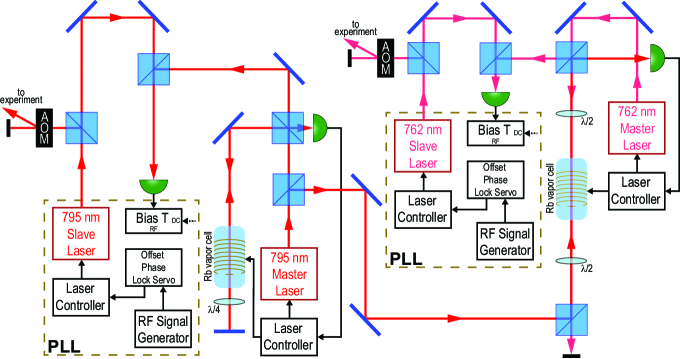
Figure 2: Phase-locked loops for frequency control of excitation lasers.

Our experiment relies on linear scanning of both the 795-nm and 762-nm probe lasers over wide spectral ranges. Linearity of the laser scans is crucial for measurements of $\frac{d\Delta_{762}^{F^{\prime}}}{d\Delta_{795}^{F^{\prime}}}$ for determining the $5D_{3/2}$ dynamic polarizability, and for measurement of the photoionization cross section. Usually, linear current or linear voltage control of the laser current or the piezo-electric (PZT) in an external-cavity diode laser does not result in accurate, linear scans over ranges of several GHz. For this reason, we lock the probe lasers (which we denote as “slave lasers” in this section) relative to fixed-frequency master lasers that are frequency-stabilized to atomic references.

The complete schematic for our optical phase-locked loops (PLLs) is depicted in Fig. 2. The master cateye-etalon diode laser (CEDL) operating at $795$ nm is peak-locked to the ⁸⁷Rb $F=2\rightarrow F^{\prime}=1$ hyperfine transition of the D1 line with saturation-absorption spectroscopy (SAS) in a $3$ cm long vapor cell Steck (2021). Peak locking is achieved through the creation of an error signal by means of dithering the current sent through coils wrapped around a rubidium vapor cell at a frequency of $250$ kHz. The resulting SAS is modulated through the Zeeman effect at $250$ kHz. A portion of the 795-nm master CEDL is sent through a separate vapor cell and counterpropagates with a beam from the 762-nm master CEDL in order to provide electromagnetically induced transparency (EIT) spectroscopy of the ⁸⁷Rb $5P_{1/2}\rightarrow 5D_{3/2}$ line upon photodetection of the 795-nm beam. In this spectrum, the hyperfine transitions of the $5D_{3/2}$-line are resolvable. We stabilize the 762-nm, master CEDL to the ⁸⁷Rb $F^{\prime}=1\rightarrow F^{\prime\prime}=2$ hyperfine transition of the $5P_{1/2}\rightarrow 5D_{3/2}$ EIT line with a peak lock similar to that of the 795-nm laser. The lowest achievable linewidths for both stabilized master lasers are a few $100$ kHz.

Once both master lasers are-frequency stabilized, we combine them with their corresponding slave lasers on fast photodiodes (several GHz bandwidth). The resulting beat signals, picked off with a bias-T, are demodulated with RF signal generators and sent to high-bandwidth $\sim 20$ MHz offset-phase-lock servos that control the laser currents of the 795-nm and 762-nm slave lasers. The RF signal generators used for the demodulation have a frequency stability of $<$ 1 kHz. By scanning the frequency of the RF signal generators while the slave lasers are phase-locked, we are able to perform GHz-long linear scans of the two probe lasers with sub-MHz resolution.

I.3 Simulation

We simulate the double-resonant two-photon laser spectrum by considering stationary atoms within a one-dimensional 1064-nm optical lattice with a maximum 5$S_{1/2}$ AC shift of -254 MHz, as determined from experimental spectra. The distribution of atoms as a function of the 5$S_{1/2}$ AC shift, $P(\Delta_{5S_{1/2}})$, is spectroscopically measured and entered into the simulation. The atomic quantization axis is along the lattice propagation direction $\bf{\hat{z}}$. The 1064-nm, $795$-nm and $762$-nm lasers are linearly polarized along $\bf{\hat{y}}$, $\bf{\hat{x}}$ and $\bf{\hat{x}}$, respectively, as in the experiment. We represent the Hamiltonian in the basis $\{|5S_{1/2},m_{j},m_{i}\rangle,|5P_{1/2},m_{j},m_{i}\rangle,|5D_{3/2},m_{j},m_{i}\rangle\}$ for ⁸⁵Rb, with all 48 electronic and nuclear magnetic sublevels of the system included.

We include the hyperfine interaction Steck (2021) and the light-shift interaction, given by Eq. 1 in the main text multiplied by $-E_{L}^{2}/4$, with local lattice electric-field amplitude $E_{L}$. For the hyperfine $A$ constants of $5S_{1/2}$ and $5P_{1/2}$ we use data from Steck (2021), and for the hyperfine $A$ and $B$ constants of $5D_{3/2}$ we use values from Nez et al. (1993). For the known AC polarizabilities we enter $\alpha^{S}_{5S_{1/2}}=687.3$ Arora and Sahoo (2012) and $\alpha^{S}_{5P_{1/2}}=-1226$ Neuzner et al. (2015), in atomic units. For $\alpha^{S}_{5D_{3/2}}$ and $\alpha^{T}_{5D_{3/2}}$ we may enter, for instance, our experimental values of $-524$ and 0, respectively.

The full Hamiltonian is diagonalized for 1000 equidistant intensity steps ranging from 0 to the intensity value at the anti-nodes of the lattice. This yields three blocks of lattice-mixed eigenstates, for the $5S_{1/2}$, $5P_{1/2}$ and $5D_{3/2}$ levels, respectively. The atoms are assumed to be initially equally distributed over the $F=3$-like states of the $5S_{1/2}$ ground manifold, with an overall weighting over the 1000 intensity steps according to the measured $P(\Delta_{5S_{1/2}}$).

The photoionization (PI) rate of the 20 lattice-mixed $5D_{3/2}$ states follows from shell-averaged PI cross section, $\sigma$, which is an input parameter that we may set, for instance, at $40\leavevmode\nobreak\$Mb. The distribution of the lattice-mixed states over the electronic magnetic sublevels then yields state-dependent PI cross sections, $\sigma_{k}$, that depend somewhat on the lattice-mixed $5D_{3/2}$ states, labeled $k=1,...,20$. The state-dependent PI rates then are $\Gamma_{PI,k}=\sigma_{k}I/(\hbar\omega_{L})$, with local light intensity $I$ and lattice angular frequency $\omega_{L}$.

Since the intensities of the excitation beams are near or below the respective saturation intensities, and since the upper (762-nm) transition is heavily broadened by PI of the $5D_{3/2}$ levels, the signals can be approximated by two-dimensional spectral profile functions $S(\Delta_{795},\Delta_{762})$ that are mildly saturated Lorentzians with a width near 6 MHz along $\Delta_{795}$, and PI-broadened Lorentzians with intensity- and state-dependent frequency linewidths $\Gamma_{PI,k}/(2\pi)$. The entire spectrum is then assembled by taking a weighted sum of profile functions centered at the detunings of the lattice-shifted lower and upper transitions along the $\Delta_{795}$- and $\Delta_{762}$-directions, respectively, and weighting factors given by the product of the line strengths of the lower and upper transitions, which are computed for the given probe light polarizations. An underlying assumption here is that every atom excited into a $5D_{3/2}$ level is photoionized. This assumption is very well satisfied due to the fact that our PI rates range up into the $10^{9}\leavevmode\nobreak\$s^-1 range. The two-dimensional spectra obtained by this procedure are then finally summed over the 1000 sampled intensity values, which a weighting function that follows from the measured lower-transition AC-shift profile $P(\Delta_{5S_{1/2}})$ entered into the simulation.

The simulations, an example of which is shown in Fig. 2(b) of the main text, qualitatively reproduce the measurements very well. The qualitative agreement in signal strengths of the F’=2 and F’=3 branches is an indicator that optical pumping plays no or only a small role in the measurement. Hence, our measured $\sigma$-value is expected be close to what it would be for an ideally isotropic atom sample. Further, the simulated spectral lines along $\Delta_{762}$ can be fitted in a way analogous to the processing of the experimental data in order to find line centers and linewidths from the simulation, and to deduce values for the polarizability $\alpha^{S}_{5D_{3/2}}$ and the PI cross section $\sigma$. For simulation input values $\alpha^{S}_{5D_{3/2}}=-524$ and $\alpha^{T}_{5D_{3/2}}=0$, the value of $\alpha^{S}_{5D_{3/2}}$ deduced from Lorentzian fits of the simulated spectra and from Eq. 3 in the main text is found to be $\alpha^{S}_{5D_{3/2}}=-523$. Further, the deduced values of $\sigma$ exceed the input value for $\sigma$ by only about 1.7$\%$. Hence, the simulations essentially validate the experimentally applied procedure. In light of the simulation result, we apply a 1.7$\%$ reduction to the $\sigma$-value deduced from the experimental spectra to arrive at our final experimental estimate of $\sigma=44(1)$ Mb.

References

- Chen et al. (2014) Y.-J. Chen, S. Zigo, and G. Raithel, Phys. Rev. A 89, 063409 (2014).
- Drever et al. (1983) R. W. P. Drever, J. L. Hall, F. V. Kowalski, J. Hough, G. M. Ford, A. J. Munley, and H. Ward, Appl. Phys. B 31, 97 (1983).
- Black (2001) E. D. Black, Am. J. Phys. 69, 79 (2001).
- Steck (2021) D. A. Steck, “Rubidium 85 D line data,” (revision 2021).
- Nez et al. (1993) F. Nez, F. Biraben, R. Felder, and Y. Millerioux, Opt. Comm. 102, 432 (1993).
- Arora and Sahoo (2012) B. Arora and B. K. Sahoo, Phys. Rev. A 86, 033416 (2012).
- Neuzner et al. (2015) A. Neuzner, M. Körber, S. Dürr, G. Rempe, and S. Ritter, Phys. Rev. A 92, 053842 (2015).