Embracing the Dark Knowledge: Domain Generalization Using Regularized Knowledge Distillation

Abstract.

Though convolutional neural networks are widely used in different tasks, lack of generalization capability in the absence of sufficient and representative data is one of the challenges that hinders their practical application. In this paper, we propose a simple, effective, and plug-and-play training strategy named Knowledge Distillation for Domain Generalization (KDDG) which is built upon a knowledge distillation framework with the gradient filter as a novel regularization term. We find that both the “richer dark knowledge” from the teacher network, as well as the gradient filter we proposed, can reduce the difficulty of learning the mapping which further improves the generalization ability of the model. We also conduct experiments extensively to show that our framework can significantly improve the generalization capability of deep neural networks in different tasks including image classification, segmentation, reinforcement learning by comparing our method with existing state-of-the-art domain generalization techniques. Last but not the least, we propose to adopt two metrics to analyze our proposed method in order to better understand how our proposed method benefits the generalization capability of deep neural networks.

1. Introduction

Recently, convolution neural networks are widely used in different tasks and scenarios thanks to the development of machine learning and computing devices. However, one of the challenges that hinders the practical application of the convolution neural network model is the lack of generalization capability in the absence of sufficient and representative data (Zhang et al., 2016; Kawaguchi et al., 2017). To overcome such limitation, domain adaptation (DA) have been widely studied under the assumption that a small amount of labeled target domain data or unlabeled target domain data can be obtained during the training stage.

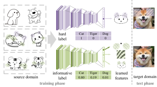
Figure 1. A motivating example of cat recognition. If the source domain data is biased, e.g., only the cat’s ears are triangular, the model using hard labels will easily overfit to the feature of triangle ear which is not domain invariant. However, if the student model uses the informative soft label from the teacher, it has to learn more general features such as the whiskers and stripes that are shared between cats and tigers and then predict the category using the combination of these features. For a dog image from the unseen domain also with triangle ears, the network trained with the hard labels may be wrongly activated.

However, in some cases, the target domain data may not always be available. As such, directly training on the source domain can lead to an overfitting problem. In other words, we can observe a significant performance drop when testing on the target domain. Domain generalization (DG) is one research direction that aims to utilize multi-source domains to train a model that is expected to be generalized better on the unseen target domains. The core idea of existing methods are either to align the features of source domains to a pre-defined simple distribution, to learn a domain invariant feature distribution (Yang and Gao, 2013; Muandet et al., 2013; Li et al., 2018a), or to conduct data augmentation (e.g., data enhancement (Wang et al., 2020; Zhang et al., 2020), generative adversarial network (GAN) based methods (Volpi et al., 2018; Zhou et al., 2020a)) on source domains. In addition, there are also some efforts using the meta-learning based method to simulate the domain gap between the source and unseen target domain. However, the aforementioned techniques inevitably face the problem of overfitting on the source domain due to the inability to access the target domain data. It is still an open problem on how to learn a universal feature representation through the aforementioned techniques that the latent features of target lie on a similar feature distribution compared with the latent features of source domains. As such, the generalization performance in the target domain may not be guaranteed due to the distribution mismatch.

Figure 2. The impact of task difficulty on the generalization performance on the source and unseen target domains. We change the ratio $\lambda$ of the noise label (the label is fixed when start training) to change the difficulty of the task (Zhang et al., 2016; Nettleton et al., 2010). The experiments were done using Digit-Five (Peng et al., 2019) benchmark and we set syn as the target domain. The network is weak to predict the randomly initialized labels which are inconsistent with the inductive preference of the model, i.e., the recognition task becomes difficult when increasing $\lambda$.

Our motivation comes from the observation that if the task is difficult for the model, i.e., the mapping from the input space to the label space is difficult to learn, the performance of the model in the target domain may have a large drop owing to the overfitting in source domains even if the performance on the source domains is still acceptable. One illustrative example to verify our observation can be seen in Fig. 2. By involving more noisy labels on the source domain, the learning task of the model also becomes difficult (Zhang et al., 2016; Nettleton et al., 2010) and we find it further deteriorates the performance of the model on the target domain. To this end, we make the assumption that the generalization performance of the model in the unseen target domain can benefit from the easy tasks. In particular, we proposed a framework named knowledge distillation for domain generalization (KDDG) with a novel gradient regularization to decrease the difficulty of the task. The motivation is mainly in two folds. 1) we leverage the advantage of knowledge distillation to provide the student with more informative labels which make the training easier (Phuong and Lampert, 2019; Hinton et al., 2015), where the rationales are illustrated in Fig. 1. We also provide a preliminary study in Fig. 3 using class activation map (CAM) (Zhou et al., 2016). We observe that our proposed method can help the student network to learn more general and comprehensive features, e.g., the legs and the body of the dog which are ignored by directly training the model with one-hot ground truth labels. 2) the gradient filter we proposed relaxes the objective of IRM that further makes the task easier (which is analyzed in Sec. 3.4 in details) and avoid the student model from completely imitating the teacher (Phuong and Lampert, 2019), such that better generalization can be further guaranteed. We show that our proposed method can outperform existing state-of-the-art domain generalization techniques on different tasks including image classification, segmentation, reinforcement learning. We further propose to adopt two different metrics, namely cumulative weight distance and mutual information, to explain the effectiveness of our proposed method. The main idea is to measure the difficulty of the task and quantify the domain-specific information. We show that our proposed method KDDG can make the task easier to train and allow the student network to learn fewer domain-specific features, which further justify our assumption to tackle the problem of domain generalization through knowledge distillation. In summary, we make the following contributions,

1. We propose to tackle the problem of domain generalization from a perspective of task difficulty and reveal that better generalization capability can be achieved if the learning task is easier.

2. We propose a simple, effective, and plug-and-play training strategy named KDDG. Experimental results on different tasks demonstrate the effectiveness of our proposed method by comparing it with the SOTA techniques.

3. Two metrics are proposed to better understand how our proposed method benefits the generalization capability of neural networks.

2. Related Work

2.1. Domain Adaptation and Generalization

How to alleviate the performance degradation caused by the domain gap between the training and test data has always been a hot research pot. One direction is to rely on unlabeled test data (a.k.a., target domain data) and apply domain adaptation (DA) or transfer learning (Huang et al., 2006; Pan and Yang, 2009; Li et al., 2020a), which can be roughly divided into two categories, namely subspace learning based methods and instance re-weighting (Huang et al., 2006; Pan et al., 2011; Zhang et al., 2015; Ghifary et al., 2017). In addition, deep learning based methods also demonstrate their effectiveness by feature alignment using different methods such as Maximum Mean Discrepancy (MMD) (Long et al., 2015) and adversarial based training (Ganin et al., 2016; Tzeng et al., 2017; Bousmalis et al., 2017; Hoffman et al., 2018).

The setting of domain generalization (DG) is similar but more challenging than the setting of domain adaptation because we cannot get any information from the target domain in the training phase. Part of the current DG methods borrow the idea from DA, e.g., domain invariant feature and feature alignment. For example, for domain invariant feature-based methods, (Yang and Gao, 2013) aimed to use Canonical Correlation Analysis (CCA) to obtain the shareable information, (Muandet et al., 2013) proposed a domain invariant analysis method which also used MMD and was further extended by (Li et al., 2018a, 2020b). Multi-task auto-encoder was also used to learn shareable feature representations (Ghifary et al., 2015). In addition, different regularization methods were proposed, e.g., low-rank regularization was used in (Xu et al., 2014; Li et al., 2017) to extract the invariant embedding, the puzzle task (Carlucci et al., 2019) was used to learn a model with good generalization performance. Meta-based methods (Li et al., 2018b; Balaji et al., 2018) can be also treated as a kind of regularization, e.g., (Li et al., 2018b) used the second derivative as a regular term and (Balaji et al., 2018) directly learned a regularization network. However, we may still not be able to guarantee that the embedding from target domains share the same subspace with that of the source domains through the aforementioned domain invariant feature learning based methods since the learned classifier can be overfitted to the source domains. In addition, the regularization may make the learning task difficult which further increases the risk of overfitting in the source domains. There also exists some works using data augmentation based techniques (Volpi et al., 2018; Zhou et al., 2020a; Wang et al., 2020). For example, (Zhou et al., 2020a) used an adversarial generative model to generate some samples that are out of the source domains to improve the generalization capability of the neural network. However, if the distribution of the newly generated data is not similar to that of the target domain, it may have a negative impact on the model. In addition, it may be difficult to generate samples out of the convex set of the source domains (Berthelot et al., 2019).

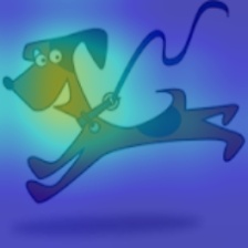
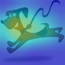
(a) cartoon

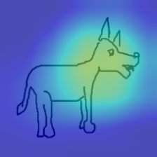
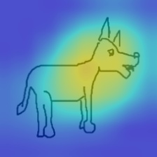
(b) sketch

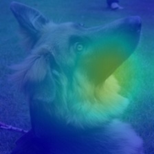
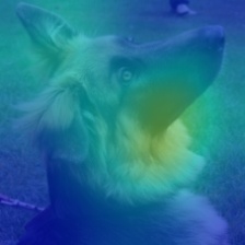
(c) photo

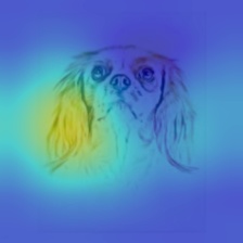
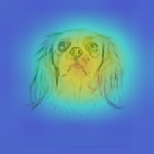
(d) painting

Figure 3. The visualization of the class activation map (Zhou et al., 2016) from source and target domains using PACS benchmark. The first row is the baseline method DeepAll and the second row is our method KDDG. The first three columns are source domains and the last is the unseen target domain.

2.2. Knowledge Distillation

To the best of our knowledge, knowledge distillation (KD) was first designed for model compression (Buciluǎ et al., 2006; Sau and Balasubramanian, 2016), which aims to make the output of the new model (student) similar to that of the previous model (teacher model) meanwhile decrease the size of the student one. In (Hinton et al., 2015; Luo et al., 2016), it has been shown that training the student model with “dark knowledge” by KD can lead to better performance compared with directly training with one-hot ground truth. Besides, it has also been shown that KD can benefit nature language processing (Li et al., 2014; Zhao et al., 2019). In the area of reinforcement learning, knowledge distillation is also known as policy distillation, which can be applied for model compression, network training acceleration, or multiple agent models merging (Rusu et al., 2015; Parisotto et al., 2015; Yin and Pan, 2017). Comparing with the application of KD, the theoretical analysis (Phuong and Lampert, 2019; Lopez-Paz et al., 2015; Cheng et al., 2020; Müller et al., 2019) is relatively deficient and mainly focus on the characteristics such as the convergence (Phuong and Lampert, 2019). While there exist some works linking KD with the generalization capability of neural network (e.g., (Phuong and Lampert, 2019; Müller et al., 2019)), they mainly focus on analyzing the generalization capability of the model using the same dataset or data distribution, e.g., the upper bound of the transfer risk (Phuong and Lampert, 2019). Different from the previous work, we explore and analyze KD from a new perspective by focusing on the setting of domain generalization where the testing data are collected from a different distribution compared with the training data.

3. Methodology

3.1. Knowledge Distillation

Before introducing our proposed method, we first revisit the idea of knowledge distillation (Hinton et al., 2015). Specifically, in order to obtain the soft label, temperature $\tau$ is introduced as a hyper-parameters to soften the vanilla softmax distribution, which is given as

(1) $$p^{i}(x;\tau)=softmax(s(x);\tau)=\frac{e^{s_{i}(x)/\tau}}{\sum_{k}e^{s_{k}(x)/\tau}}$$

where $s_{i}(x)$ is the score logit from the sample $x$ of class $i$. Subsequently, the KL-divergence is used as the distillation loss $L_{kd}$ to measure the difference between the teacher and student:

(2) $$L_{kd}=-\tau^{2}\mathbb{E}_{x\sim D_{s}}\sum_{i=1}^{C}p_{t}^{i}(x;\tau)log(p_{s}^{i}(x;\tau))$$

where $p_{t}$ and $p_{s}$ denote the softened probability from the teacher and student network respectively, $C$ is the total number of the categories, $D_{s}$ indicates the distribution of all source domain data by concatenating them together. Here, the coefficient $\tau^{2}$ is used to balance the magnitude of the gradient (Hinton et al., 2015) between hard and soft label. The loss function for the student network is as follows:

(3) $$L_{vanilla}=\lambda_{1}L_{ce}+\lambda_{2}L_{kd}$$

where $L_{ce}$ is the standard cross-entropy, $\lambda_{1}$ and $\lambda_{2}$ are balancing weight.

3.2. Gradient Filter

We further propose a novel gradient regularization to improve the generalization capability of the network. Without loss of generality, we use the classification task to illustrate the gradient filter $f$. Assuming that $p(x_{i})$ denote the softmax output vector of the student network from the sample $x_{i}$, $p^{k}(x_{i})$ represents the probability value of the sample $x_{i}$ with respect to its ground truth category $k$ (abbreviated as $p$). We can define the gradient filter $f$ as

(4) $$f(\omega)=\left\{\begin{matrix}\omega&p\leq\eta\\ (\frac{\eta+1-2p}{1-\eta})^{2}\omega&\eta<p\leq\frac{1+\eta}{2}\\ 0&p>\frac{1+\eta}{2}\\ \end{matrix}\right.$$

where $\omega$ denotes gradient and $\eta$ is a hyper-parameter that controls the intensity of the filter. Noted that we can also apply the operation $f$ on the empirical risk of a sample, as our proposed GradFilter can be treated as imposing weight on the loss function.

The significance of $f$ comes from mainly two folds, 1) we can prevent the student network from being too similar to the teacher network (Phuong and Lampert, 2019), such that the risk of overfitting to teacher network can be reduced; 2) by filtering out the gradient corresponding to high score output, we can avoid the problem of over-confidence (Guo et al., 2017; Müller et al., 2019) and make the optimization task easier by relaxing the objective of IRM which will be further discussed in Sec. 3.4.

3.3. Knowledge Distillation for DG

Now we introduce our proposed method built upon knowledge distillation with gradient filter regularization. Specifically, at each iteration, the gradient filter inspects the confidence of each sample and decrease the gradient weight of the sample which has a confidence score higher than a pre-defined threshold (by setting the corresponding loss to zero). Thus, the integrated loss for domain generalization can be formulated as

(5) $$L_{kd}^{f}=-\tau^{2}\mathbb{E}_{x\sim D_{s}}\epsilon(f(\sum_{i=1}^{C}p_{t}^{i}(x;\tau)log(p_{s}^{i}(x;\tau))))$$

(6) $$L_{ce}^{f}=-\mathbb{E}_{x\sim D_{s}}f(\sum_{i=1}^{C}(y^{i}log(p_{s}^{i}(x)))$$

where $y^{i}$ denotes the ground truth of the sample $x$ for class $i$. $\epsilon$ is defined as follows to avoid the bad effect from the wrong predict from the teacher

(7) $$\epsilon(l)=\left\{\begin{matrix}l&\upsilon(p_{t}(x_{i}))=y_{i}\\ 0&\text{otherwise}\end{matrix}\right.$$

where $p^{k}_{s}(x_{i})$ and $p_{t}$ represent the probability value of the sample $x_{i}$ with the class index $k$ from the student network and probability vector from the teacher network respectively, $\upsilon$ is an operation that returns the predicted label according to the probability vector. The final objective for KDDG can be represented as

(8) $$L_{KDDG}=\lambda_{1}L_{kd}^{f}+\lambda_{2}L_{ce}^{f}.$$

For KD, we set $\tau$ to 2. We also set $\lambda_{1}$ and $\lambda_{2}$ to 0.5 so that we have roughly the same magnitude of the gradient for fair comparison and easy analysis.

3.4. Discussion

To further understand the rationale and effectiveness of gradient filter we proposed, we give a view from the perspective of invariant risk minimization (IRM) (Ahuja et al., 2020; Arjovsky et al., 2019), which is for generalization analysis of the classifier across multiple domains.

According to IRM, the task of DG can be treated as to find a representation $\Phi$ such that the optimal classifier given $\Phi$ is invariant across different domains. More specifically, for a feature extractor $\Phi$, there exists an invariant predictor $w$ if this predictor achieves the best performance among all the domains. In (Ahuja et al., 2020; Arjovsky et al., 2019), the authors proposed to find the optimal $\Phi$ and $w$ as

(9) $$\underset{\Phi\in\mathcal{H}_{\Phi},w\in\mathcal{H}_{w}}{\min}\underset{d\in\mathcal{D}}{\sum}\mathcal{L}^{d}(w\circ\Phi)$$

$$\text{ s.t. }w\in\arg\underset{\bar{w}\in\mathcal{H}_{w}}{\min}\mathcal{L}^{d}(\bar{w}\circ\Phi),\forall d\in\mathcal{D}$$

where $\mathcal{L}^{d}$ is the empirical risk in the domain $d$ and $\mathcal{D}$ represents all the domains, and the solution space of $(w,\Phi)$ can be defined as $\mathcal{S}^{IV}$.

Unlike the previous works about IRM (Ahuja et al., 2020; Arjovsky et al., 2019), our GradFilter can be treated as to conduct solution space transformation on $\mathcal{S}^{IV}$. By applying GradFilter operation, Eq. 9 can be reformulated as

(10) $$\underset{\hat{\Phi}\in\mathcal{H}_{\Phi},\hat{w}\in\mathcal{H}_{w}}{\min}\underset{d\in\mathcal{D}}{\sum}f(\mathcal{L}^{d}(\hat{w}\circ\hat{\Phi}))$$

$$\text{ s.t. }\hat{w}\in\arg\underset{\tilde{w}\in\mathcal{H}_{w}}{\min}f(\mathcal{L}^{d}(\tilde{w}\circ\Phi)),\forall d\in\mathcal{D}$$

where $f$ is the GradFilter operation defined in Eq. 4 which avoid the model over-confidence in the source domains.

Our proposed GradFilter can be interpreted as to relax the objective of IRM. If directly optimizing Eq. 9, it may be hard to find a solution which satisfies both the objective and the regularization term, as there may not exist an intersection among the solution set of each source domain. By relaxing the objective, we make the optimization task easier, i.e., it is more likely that there exists an overlap region among solution space between source domains. Thus, our proposed method can be interpreted as an alternative solution for Eq. 9. More details can be found in the supplementary materials.

(a) Digit-Five(Peng et al., 2019)

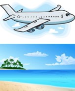
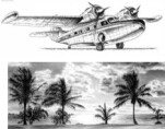
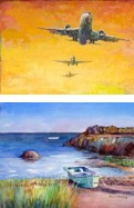
(b) mini-DomainNet (Peng et al., 2019; Zhou et al., 2020b)

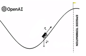
(c) Mountain-Car (Brockman et al., 2016)

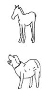
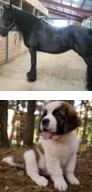
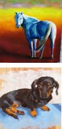
(d) PACS (Li et al., 2017)

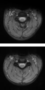
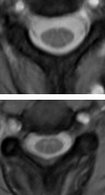
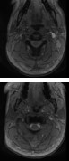
(e) gray matter segmentation (Prados et al., 2017)

Figure 4. An illustration of domain generalization benchmarks used for evaluation. Each column represents a domain and the data are randomly sampled except the reinforcement learning task Mountain-Car where the domain gap is concentrated in the different gravitational constant.

4. Experiments

We evaluate our methods on different domain generalization benchmarks, including Digit-Five (Peng et al., 2019), PACS (Li et al., 2017), mini-domainnet (Peng et al., 2019; Zhou et al., 2020b), gray matter segmentation task (Prados et al., 2017) and mountain car (Brockman et al., 2016). Examples of each benchmark are shown in Fig. 4. For all the experiments, we use the same architecture for both teacher and student network. In addition, the gradient filter is only used when training the student network based on its output. Due to the limited space, more details about the experiments are in the supplementary material.

4.1. Digits-Five

Digits-Five is a benchmark used by (Peng et al., 2019), which is composed of MNIST-M, MNIST, SVHN, USPS and SYN with different backgrounds, fonts, styles, etc.

Settings: We follow the experiment settings in (Peng et al., 2019) except that we assume the target domain is unavailable during training. More specifically, we adopt a standard leave-one-domain-out manner. For the source domains, 80% of the samples are used for training and 20% for validation. All the samples in the target domain are used for testing. We follow (Peng et al., 2019) to convert all image samples with the resolution of $32\times 32$ in RGB format. We use the same backbone network for all methods which include three convolutional blocks and two FC layers. Each convolutional block contains a $3\times 3$ convolutional layer, a batch normalization layer, a Relu layer, and a $2\times 2$ max-pooling layer. The SGD is used with an initial learning rate of 0.05 and a weight decay of 5e-4 for 30 epochs. The cosine annealing scheduler is used to decrease the learning rate.

Results: We compare our methods with several competitive models including MLDG (Li et al., 2018b), JiGen (Carlucci et al., 2019), MASF (Dou et al., 2019) and RSC (Huang et al., 2020). We report the baseline results in Table 1 by tuning the hyper-parameters in a wide range. As we can observe, our method achieves the best results which prove the effectiveness of our proposed method. In addition, using the knowledge distillation alone also has some improvement which further verifies our motivation.

	MM	MNIST	USPS	SVHN	SYN	Avg.
DeepAll	66.3	96.7	94.1	82.1	88.9	85.6
MLDG (Li et al., 2018b)	67.9	97.3	94.7	83.9	89.1	86.6
JiGen (Carlucci et al., 2019)	67.8	97.8	95.9	84.7	89.6	87.2
MASF (Dou et al., 2019)	69.2	98.6	96.3	84.4	90.1	87.7
RSC (Huang et al., 2020)	69.8	98.3	96.1	84.1	89.9	87.6
Distill	69.7	99.2	97.3	84.7	90.4	88.3
KDDG(Ours)	70.5	99.1	97.6	85.5	90.6	88.7

Table 1. Evaluation of DG on the Digit-Five benchmark. The average target domain accuracy of five repeated experiments is reported. MM and SYN are abbreviations for MNIST-M and Synthetic Digits.

4.2. PACS

PACS (Li et al., 2017) is a standard benchmark for domain generalization which includes 4 different domains: photo, sketch, cartoon, painting. There are 7 categories in the dataset and 9991 images in total.

Settings: Following the experiment settings in (Carlucci et al., 2019), we use the ImageNet pre-trained ResNet18 as the backbone network for all methods. The samples from source domains are divided into training (90%) and validation (10%) using the official train-val splits. All the images from the target domain are used for test. SGD is used to train all the networks with an initial learning rate of 5e-4, batch size of 16, and weight decay 5e-4 for 25 epochs. The learning rate is decreased to 5e-5 at the $20$th epoch. It is worth noting that we use the same data argumentation for all methods which include random crop on images with a scale factor of 1.25 and random horizontal flip. We do not use the augmentations, e.g., random gray scale, considering that it can introduce the prior knowledge of specific domain information, e.g., the samples in the sketch domain are all grayscale which are not available in the DG setting.

Results: To compare the performance of different methods, we report the top 1 classification accuracy in the unseen target domain. We repeat the experiment for 5 times and report the average target domain accuracy at the last epoch. Several state of the art methods are used for comparison, including CCSA (Yoon et al., 2019), MLDG (Li et al., 2018b), CrossGrad (Shankar et al., 2018), eta. The results are shown in Table 2. It is worth noting that our method is different from MASF (Dou et al., 2019) which minimizes the divergence of the class-specific mean feature vectors between meta-train and meta-test domains. Specifically, we consider to conduct knowledge distillation in an one-one correspondence manner based on the same input between teacher and student network, which may avoid negative transfer and we also empirically find that if can lead to better performance.

	Art	Cartoon	Photo	Sketch	Avg.
DeepAll	77.0	75.9	95.5	70.3	79.5
CCSA (Yoon et al., 2019)	80.5	76.9	93.6	66.8	79.4
MLDG (Li et al., 2018b)	78.9	77.8	95.7	70.4	80.7
CrossGrad (Shankar et al., 2018)	79.8	76.8	96.0	70.2	80.7
JiGen (Carlucci et al., 2019)	79.4	75.3	96.0	71.6	80.5
MASF (Dou et al., 2019)	80.3	77.2	93.9	71.7	81.0
Epi-FCR (Li et al., 2019)	82.1	77.0	93.9	73.0	81.5
RSC (Huang et al., 2020)	79.5	77.8	95.6	72.1	81.2
KDDG(Ours)	81.0	78.7	96.0	72.3	82.0

Table 2. Evaluation of DG on the PACS benchmark. The average target domain accuracy of five repeated experiments is reported.

target	DSC	CC	JI	TPR	ASD
1	0.8560	65.34	0.7520	0.8746	0.0809
2	0.7323	26.21	0.5789	0.8109	0.0992
3	0.5041	-209	0.3504	0.4926	1.8661
4	0.8775	71.92	0.7827	0.8888	0.0599
Average	0.7425	-11.4	0.6160	0.7667	0.5265

(a) DeepAll

target	DSC	CC	JI	TPR	ASD
1	0.8061	50.15	0.6801	0.8703	0.1678
2	0.8009	50.04	0.6687	0.8141	0.0939
3	0.5012	-112	0.3389	0.5444	1.5480
4	0.8686	69.61	0.7684	0.8926	0.0449
Average	0.7442	14.45	0.6140	0.7804	0.4637

(b) CCSA (Yoon et al., 2019)

target	DSC	CC	JI	TPR	ASD
1	0.8502	64.22	0.7415	0.8903	0.2274
2	0.8115	53.04	0.6844	0.8161	0.0826
3	0.5285	-99.3	0.3665	0.5155	1.8554
4	0.8938	76.14	0.8083	0.8991	0.0366
Average	0.7710	23.52	0.6502	0.7803	0.5505

(c) MASF (Dou et al., 2019)

target	DSC	CC	JI	TPR	ASD
1	0.8585	64.57	0.7489	0.8520	0.0573
2	0.8008	49.65	0.6696	0.7696	0.0745
3	0.5269	-108	0.3668	0.5066	1.7708
4	0.8837	73.60	0.7920	0.8637	0.0451
Average	0.7675	19.96	0.6443	0.7480	0.4869

(d) MLDG (Li et al., 2018b)

target	DSC	CC	JI	TPR	ASD
1	0.8708	69.29	0.7753	0.8978	0.0411
2	0.8364	60.58	0.7199	0.8485	0.0416
3	0.5543	-71.6	0.3889	0.5923	1.5187
4	0.8910	75.46	0.8039	0.8844	0.0289
Average	0.7881	33.43	0.6720	0.8058	0.4076

(e) LDDG (Li et al., 2020c)

target	DSC	CC	JI	TPR	ASD
1	0.8745	70.75	0.7795	0.8949	0.0539
2	0.8229	56.71	0.6997	0.8226	0.04901
3	0.5676	-63.1	0.3866	0.5904	1.2805
4	0.8894	75.06	0.8011	0.9222	0.0377
Average	0.7886	34.86	0.6667	0.8075	0.3553

(f) KDDG (Ours)

Table 3. Domain generalization results on gray matter segmentation task.

4.3. Mini-DomainNet

We then consider mini-DomainNet (Zhou et al., 2020b), which is a subset of DomainNet (Peng et al., 2019) for evaluation. It contains 4 domains, namely sketch, real, clipart and painting, with more than 140k images in total.

Settings: We use SGD with momentum as the optimizer. The initial learning rate is 5e-3 and is decreased using the cosine annealing rule (Loshchilov and Hutter, 2016). The batch size is 128 with a random sampler from the concatenated source domains. Resnet-18 is used as the backbone network for all competitors and we train the model for 60 epochs. We use the same data augmentation for all the methods, including random flip and random crop with a scale factor of 1.25. We adjusted the hyperparameters for the competitors in a wide range and report the best results we can achieve here.

Results: We repeat the experiments for 3 times and report the average accuracy in Table 4. We can find that our method has an improvement in a clear margin compared with other methods in the mini-DomainNet benchmark which is much larger than PACS. Such observation further justifies the significance of our proposed method to handle large-scale data.

	Clipart	Real	Painting	Sketch	Avg.
DeepAll	62.86	58.73	47.94	43.02	53.14
MLDG (Li et al., 2018b)	63.54	59.49	48.68	43.41	53.78
JiGen (Carlucci et al., 2019)	63.84	58.80	49.40	44.26	54.08
MASF (Dou et al., 2019)	63.05	59.22	48.34	43.67	53.58
RSC (Huang et al., 2020)	64.65	59.37	46.71	42.38	53.94
KDDG(Ours)	65.80	62.06	49.37	46.19	55.86

Table 4. Evaluation of DG on mini-DomainNet benchmark.

4.4. Gray Matter Segmentation

We further evaluate our proposed method on gray matter segmentation task (Li et al., 2020c; Prados et al., 2017) which aims to segment the gray matter area of the spinal cord for medical diagnosis. We use the data from spinal cord gray matter segmentation challenge (Prados et al., 2017) which are collected from four different medical centers with different MRI scanner parameters, e.g., different resolution from $0.25\times 0.25\times 2.5mm$ to $0.5\times 0.5\times 5mm$, the flip angle from $7^{\circ}$ to $35^{\circ}$, different coil type. These differences lead to four different domains named ’set1’, ’set2’, ’set3’, and ’set4’.

Settings: We use the same 2D-UNet (Ronneberger et al., 2015; Li et al., 2020c) as the backbone for a fair comparison. A two-stage strategy in a coarse-to-fine manner is adopted following (Prados et al., 2017; Li et al., 2020c). More specifically, we first segment the area of the spinal cord and then extract the area of gray matter from the spinal cord.

Results: We compare our method with state of the art domain generalization methods, including MASF (Dou et al., 2019), MLDG (Li et al., 2018b), CCSA (Yoon et al., 2019), LDDG (Li et al., 2020c), using different metrics including three overlapping metrics: Dice Similarity Coefficient (DSC $\uparrow$), Conformity Coefficient (CC $\uparrow$), Jaccard Index (JI $\uparrow$); one statistical based metrics: True Positive Rate (TPR $\uparrow$); one distance based metric based on 3D: Average surface distance (ASD $\downarrow$). $\uparrow$ means the higher the better, $\downarrow$ means the lower the better. The results are shown in Table 3 and Fig. 5. According to the results, we can find that our method has the best performance overall comparing with the latest SOTA works.

4.5. Mountain Car

Besides evaluating on the benchmark datasets in computer vision, we are also interested in analyzing our proposed KDDG in the reinforcement learning task. To be specific, we use a standard reinforcement learning benchmark in OpenAI gym (Brockman et al., 2016) named mountain car. The target is to let the mountain car hit the peak with the least fuel cost with the actions “push left”, “no push”, and “push right” in the action space.

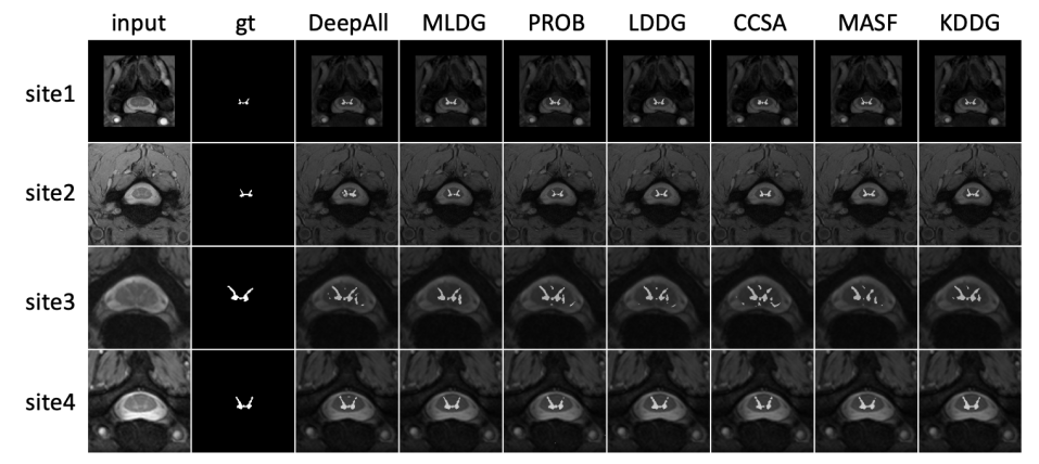
Figure 5. Qualitative comparisons. Each row represents a sample from a specific domain. Each column denotes the input, ground truth (gt) or different methods including DeepAll, MLDG (Li et al., 2018b), Probabilistic U-Net (Kohl et al., 2018) (abbreviated as PROB here), LDDG (Li et al., 2020c), CCSA (Yoon et al., 2019), MASF (Dou et al., 2019) and KDDG, respectively.

Settings: We create different domains by change the gravitational constant $g$ in the game. More specifically, $g$ is set in a range from 0.0019 to 0.0031 with a step 0.0003, which leads to 5 different environments regarded as 5 domains. We use the setting of single domain generalization here in which only one domain is used for training, where $g=0.0025$, and others are used as unseen target domains for the test. We use the DQNs as the baseline and use the same backbone for all methods. The details of our backbone can be found in the supplementary materials. We compare our method with MLDG (Li et al., 2018b) and Maximum Entropy Reinforcement Learning (MERL) based method which also encourages the output to be soft and increases the generalization ability.

Results: We repeat the experiments for 10 times and then report the average score of fuel consumption and the corresponding standard deviation in the Table 5. The smaller the value in the table, the better. It represents the amount of fuel consumption. We can find that both MLDG (Li et al., 2018b) and MERL (Haarnoja et al., 2018) have some improvement even if we use a single domain for training. We can also observe that our method has a better performance in most of the cases and has a more stable performance than the baseline method.

$g$	Baseline	MLDG (Li et al., 2018b)	MERL (Haarnoja et al., 2018)	KDDG
$0.0019$	111.8$\pm$1.84	109.9$\pm$2.43	110.2$\pm$1.92	108.7$\pm$2.23
$0.0022$	109.2$\pm$1.28	106.8$\pm$1.49	108.1$\pm$1.97	107.9$\pm$1.54
$0.0025$	113.0$\pm$6.08	110.8$\pm$7.01	112.4$\pm$8.65	109.3$\pm$4.78
$0.0028$	174.6$\pm$22.9	121.4$\pm$21.7	127.9$\pm$18.3	117.0$\pm$20.2
$0.0031$	167.7$\pm$11.0	139.8$\pm$22.1	134.8$\pm$24.6	126.8$\pm$25.9

Table 5. Single domain generalization results on the RL task moutain car. In the source domain, $g$ is set to 0.0025. The amount of fuel consumption is used as the metric (Brockman et al., 2016) for which the smaller the better.

4.6. Ablation Study

To further understand the contribution of each component, we conduct the ablation study by using the PACS benchmark. The results are shown in Table 6. We can find about 1.2% improvement from 79.5% to 80.7% in average when only using the gradient filter and 1.4% improvement when only using the vanilla knowledge distillation which is competitive to the results of some DG methods. Our proposed KDDG can achieve the best performance with 2.5% improvement in average. In addition, we also consider (Müller et al., 2019) which aims at label smoothing $y_{k}^{LS}=(1-\alpha)y_{k}+\alpha/K$ for model calibration and generalization improvement. We can find (Müller et al., 2019) slightly improve the performance by 0.5%, which is lower than using the informative label from the teacher network. Such results suggest that (Müller et al., 2019) may not be helpful with cross-domain generalization improvement.

	Art	Cartoon	Photo	Sketch	Avg.
DeepAll	77.0	75.9	95.5	70.3	79.5
SoftLabel(Müller et al., 2019)	80.4	66.8	95.8	76.9	80.0
KD	80.0	77.9	95.4	70.2	80.9
GradFilter	78.9	77.8	95.7	70.5	80.7
KDDG	81.0	78.7	96.0	72.3	82.0

Table 6. Ablation study on the PACS benchmark. KD: using vanilla knowledge distillation in Eq.3. GradFilter: only use the gradient filter without a distillation manner. KDDG: our complete version.

5. Further Analysis

To further explore the rationale of the effectiveness of our proposed method, we propose two metrics to quantify the task difficulty and the amount of superfluous domain specific information respectively.

5.1. Difficulty Quantification

5.1.1. Metric to Quantify the Difficulty

As discussed previously, there exists a connection between the task difficulty and the generalization capability of the trained model. We have shown our preliminary experiments in Fig. 2 to explore the impact of task difficulty on generalization performance by setting different noisy label levels of the ground truth. We are also interested to quantify the task difficulty to analyze how task difficulty influences the generalization capability. While there exist some works to quantify the difficulty in computer vision tasks (Tudor Ionescu et al., 2016; Nie et al., 2019), however, they mainly focus on assessing the difficulty of a single picture or of a certain area in the picture (Nie et al., 2019; Qin et al., 2019), which may not be suitable in our setting. To this end, we propose to use cumulative weight distance (CWD) to quantify the difficulty of the task, where CWD can be defined as

(11) $$\text{CWD}=\sum_{k=1}^{N}\left\|w_{k}-w_{k-1}\right\|_{2}$$

where $w_{k}$ is the parameters expanded into a vector at epoch $k$ and $w_{0}$ denotes the initial parameters vector. $N$ denotes the maximum number of epochs. We adopt the metric CWD to verify our assumption that the simpler the task is, the smaller CWD is.

5.1.2. Analysis of Results Based on the Cumulative Weight Distance

The results of CWD by varying noise level $\lambda$ are shown in Fig. 6 using the same setting as Fig. 1. We can draw the conclusion that the simpler the task, the smaller CWD and the better generalization. To further explore the impact of our method KDDG on CWD, we also conduct experiments using different components of our method. The results are shown in Table 7. We can find that KD, GradFilter, and KDDG can reduce the CWD compared with directly training with the DeepAll baseline. Such observation further verifies our assumption. It’s worth noting that there is a lower bound of CWD to learn the domain invariant feature still, so here we emphasize the difference of CWD between baseline and our methods.

	DeepAll	KD	GradFilter	KDDG
CWD	14.51	14.44	14.30	14.28

Table 7. The impact of different components on CWD.

Figure 6. The change of CWD with training using different noise level $\lambda$. We use syn in digit-five as the target domain and train the model for 50 epochs. We can find that CWD and task difficulty are positively correlated, i.e., the easier the task, the smaller CWD.

5.2. Quantification of Domain Specific Information

5.2.1. Metric Definition

We further analyze how our proposed method benefits the generalization capability of the model. Specifically, we use mutual information $I(Z,Y_{d})$ to quantify the amount of residual domain specific information where $Z$ is the latent feature space and $Y_{d}$ is the domain label space. The idea is that, the less domain-specific information contained in the feature space, the more shareable information we can obtain which benefit domain generalization.

Mutual information between $Z$ and $Y_{d}$ is defined as

(12) $$I(Z,Y_{d})=\int dy_{d}\,dz\,f(y_{d},z)\log\frac{f(y_{d},z)}{f(y_{d})f(z)}.$$

We propose to use the Monte Carlo method such that the mutual information $I(Z,Y_{d})$ in a tractable manner. Specifically, $I(Z,Y_{d})$ can be derived as

(13) $$\begin{aligned} I(Z,Y_{d})&=\int dy_{d}\,dz\,f(y_{d},z)\log\frac{f(y_{d},z)}{f(y_{d})f(z)}\\ &=\!\int\!\!dy_{d}\,dz\,f(y_{d},z)\log f(y_{d}|z)\!\\ &-\!\!\int\!dy_{d}\,f(y_{d})\log f(y_{d})\\ &=H(Y_{d})-\mathbb{E}_{z\sim f(z)}H(f(y_{d}|z)).\end{aligned}$$

To compute $I(Z,Y_{d})$, we also need to compute $f(z)$, which is the distribution of the latent feature $z$, as well as the likelihood of the domain discriminator $f(y|z)$. $f(z)$ can be computed by using the law of total probability (Zwillinger and Kokoska, 1999)

(14) $$f(z)=\sum_{i=1}^{N}f(z|x_{i})p(x_{i}),$$

where $f(z|x)$ is the conditional distribution from the feature encoding sub-network of the original model, $f(y_{d}|z)$ can be computed by using SVM with class probability (Wu et al., 2004) with five cross validation in the source domains. We empirically find that it has faster speed, higher accuracy and better stability than convolutional neural networks based domain discriminators.

5.2.2. Analysis of Results Based on Mutual Information

Now we use the metric $I(Z,Y_{d})$ to quantify the amount of domain-specific information remaining in the network. The sketch domain in the PACS benchmark is used for evaluation on account of its good discrimination. We train the models for 26 epochs and show the amount of domain-specific information $I(Z,Y_{d})$ remaining in the network in Fig. 7. As we can see, domain specific information will quickly decrease at the beginning of the training phase. However, as the training progresses, the model will inevitably overfit on the training source domains. Besides, we can also draw a conclusion from Fig. 7 that the harder the task, the more domain specific information will be learned. Last, we show the results of $I(Z,Y_{d})$ in Table 8 by considering different component. We can see that by jointly considering KD and GradFilter, more domain-specific information can be removed.

Figure 7. Trends in the amount of residual domain specific information during training under different noise level $\lambda$. Our method KDDG significantly reduce the domain specific information comparing with DeepAll.

	DeepAll	KD	GradFilter	KDDG
$I(Z,Y_{d})$	0.91	0.82	0.86	0.73

Table 8. The amount of domain-specific information remaining in the network. KD: using vanilla knowledge distillation in Eq.3 from vanilla teacher.

6. Conclusion

We address the domain generalization problem by proposing a simple, effective, and plug-and-play training strategy based on a knowledge distillation framework with a novel gradient regularization. We show that our method can achieve state-of-the-art performance on five different DG benchmarks including classification, segmentation, and reinforcement learning. We further analyze the significance and effectiveness of our method by proposing two metrics from the perspective of task difficulty and domain information.

Appendix A Further Discussion on GradFilter

A.1. An Alternative Implementation of GradFilter

In this section, we explain the advantage of our proposed GradFilter with a smooth transition (shown in Eq. 15) by comparing it with a “hard detach” formulation baseline, which is shown in Eq. 16.

(15) $$f(\omega)=\left\{\begin{matrix}\omega&p\leq\eta\\ (\frac{\eta+1-2p}{1-\eta})^{2}\omega&\eta<p\leq\frac{1+\eta}{2}\\ 0&p>\frac{1+\eta}{2}\\ \end{matrix}\right.$$

(16) $$f(\omega)=\left\{\begin{matrix}\omega&p\leq\eta\\ 0&p>\eta\\ \end{matrix}\right.$$

According to our empirical analysis, we find that a hard detach of the gradient may make the training unstable. We show one example which can cause the unstable training in Fig. 8. Comparing with the hard detach, the GradFilter we proposed avoids the abrupt changes of the loss and makes the training more stable.

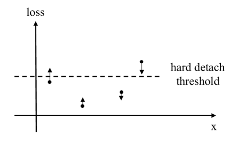
Figure 8. An illustration of a cause of instability during training. Assuming that there is a sample that has a lower confidence score than the threshold $\eta$, if we use the hard detach, i.e., the loss of the sample that has a confidence score higher than the threshold is directly set to 0, after a small update to the model, the loss may rise instantly, e.g., samples that were originally under the threshold may suddenly reach the threshold, causing the abrupt changes of loss and instability of the training.

A.2. The Choice of the Hyperparameter $\eta$

We set $\eta$ to 0.999 for all the experiments. At first glance, it may seem to be a relatively large value, but it is actually a relatively small value because of the miscalibration (Guo et al., 2017) of the neural network. A demonstration of the miscalibration is shown in Fig. 9 using PACS benchmark and select ‘sketch’ as the target domain. We can find that most of the samples have a confidence score higher than the threshold $\eta$ we set which further verifies our observation in the ablation study that using GradFilter only can also improve the performance of the model by reducing the overfitting in the source domains.

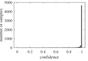
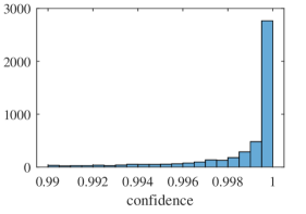
Figure 9. Confidence histograms under different bin edges. We can find that most of the samples in the training set has a confidence higher than 0.999 after training using DeepAll.

Appendix B Additional Experiments

B.1. Time and Space Complexity Analysis

We now analyze the time and space complexity of our proposed KDDG by comparing the running efficiency during the training phase with meta-based method MLDG (Li et al., 2018b), ensemble learning based method Epi-Fcr (Li et al., 2019), alignment based method MASF (Dou et al., 2019). We measure the training iteration time of networks by using the same batch size and setting as the PACS benchmark on an NVIDIA GeForce RTX 2080 Ti GPU. The results are in Table 9. As we can see, the complexity of our proposed KDDG is similar to other baseline methods, as the cost of the inference stage without gradient calculation is very small. The complexity of our method is the same as DeepAll baseline during the inference stage.

Table 9. Time and space complexity analysis

	DeepAll	MLDG	Epi-FCR	MASF	KDDG (Ours)
s/iteration	0.0319	0.2824	0.5445	0.3683	0.0382
memory used (MB)	2115	3011	5095	2779	2227

B.2. More Visualization Results

In addition to the visualization results in the paper, we also show some extra visualization results in Fig. 10 using class activation map (Zhou et al., 2016). We can find that our method tends to have a larger area of the CAM which further verifies our assumption that our method can force the student network to learn more general features to reduce the overfitting in the source domains.

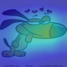
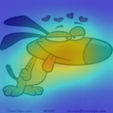
(a) cartoon

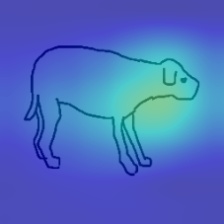
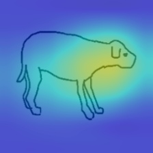
(b) sketch

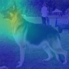
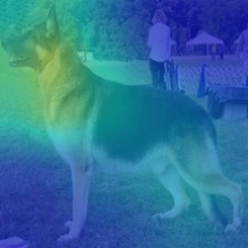
(c) photo

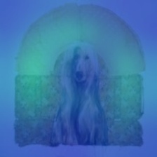
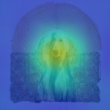
(d) painting

Figure 10. The visualization of the class activation map (Zhou et al., 2016) from source and target domains using PACS benchmark. The first row is the baseline method DeepAll and the second row is our method KDDG. The first three columns are source domains and the last is the unseen target domain.

Appendix C Experiment Details

C.1. Digits-Five

For the data augmentation, we use the same augmentation for all baselines that normalize the image with a mean of 0.5 and a standard deviation of 0.5 and then resize to the size 32 $\times$ 32. The data which only have one gray channel are first converted into RGB by copying the gray channel. Following the setting in (Peng et al., 2019), we sample 25000 images from the training data and 9000 from testing data in MINST-M, MNIST, Synthetic Digits, and SVHN. For the dataset USPS which has less than 25000 images, we repeat it for 3 times to ensure that the data is roughly balanced

C.2. Gray Matter Segmentation

We adopt the same backbone network architecture 2D-Unet with (Li et al., 2020c) that the code is released in github . We adopt the weighted binary cross-entropy as the classification loss, where the weight of a positive sample is set to the reciprocal of the positive sample ratio in the region of interest. The knowledge distillation loss is also weighted using the sample weight as above. We use Adam as the optimizer with the learning rate 1e-4. For data processing, the 3D MRI data are first sliced into 2D in axial slice view and then center cropped to 160$\times$160. In the training phase, the random crop is used which leads to the size of 144$\times$144. For evaluation, the center crop is used to resize the data to the same size. Adam optimizer is used to train the model with a learning rate of 1e-4, weight decay as 1e-8. The model is trained for 200 epochs and the learning rate is decreased 0.1 times of the original every 80 epoch. We set hyperparameter $\eta$ to 1-1e-4 for all the domains.

C.3. Mountain Car

We use the same setting for all methods. More specifically, we follow the method in (Mnih et al., 2015). Two networks are used as the action-value function and target action-value function using the same architecture which includes a single FC layer including 64 channels with a Relu activation function and two FC layers to predict the mean and the zero-center vector of the Q value separately. The state of the car is fed into the network including the position and speed. The capacity of the memory buffer is set to 500. MSE loss is used to calculate the loss in the Bellman equation. We use Adam as the optimizer with a learning rate of 1e-4 and the batch size is set to 10. The discount factor gamma is set to 0.9 and the exploration rate is set to 0.05. We train the model for 2000 episodes and merge two models every 10 episodes. As for the reward function, it is defined as the following piecewise function form

(17) $$r(p)=\left\{\begin{matrix}100&p\geq 0.5\\ 10(0.4+p)^{3}&-0.4<p<0.5\\ -0.1&p\leq-0.4\end{matrix}\right.$$

where $p$ is the position of the car returned from the environment. With regard to our method KDDG, we first do the softmax on the output of the target action-value network and then do the same operation comparing with the operation in the object recognition task.

References

- (1)
- Ahuja et al. (2020) Kartik Ahuja, Karthikeyan Shanmugam, Kush Varshney, and Amit Dhurandhar. 2020. Invariant risk minimization games. arXiv preprint arXiv:2002.04692 (2020).
- Arjovsky et al. (2019) Martin Arjovsky, Léon Bottou, Ishaan Gulrajani, and David Lopez-Paz. 2019. Invariant risk minimization. arXiv preprint arXiv:1907.02893 (2019).
- Balaji et al. (2018) Yogesh Balaji, Swami Sankaranarayanan, and Rama Chellappa. 2018. MetaReg: Towards Domain Generalization using Meta-Regularization. In NuerIPS. 998–1008.
- Berthelot et al. (2019) David Berthelot, Colin Raffel, Aurko Roy, and Ian Goodfellow. 2019. Understanding and improving interpolation in autoencoders via an adversarial regularizer. ICLR (2019).
- Bousmalis et al. (2017) Konstantinos Bousmalis, Nathan Silberman, David Dohan, Dumitru Erhan, and Dilip Krishnan. 2017. Unsupervised pixel-level domain adaptation with generative adversarial networks. In CVPR, Vol. 1. 7.
- Brockman et al. (2016) Greg Brockman, Vicki Cheung, Ludwig Pettersson, Jonas Schneider, John Schulman, Jie Tang, and Wojciech Zaremba. 2016. Openai gym. arXiv preprint arXiv:1606.01540 (2016).
- Buciluǎ et al. (2006) Cristian Buciluǎ, Rich Caruana, and Alexandru Niculescu-Mizil. 2006. Model compression. In SIGKDD.
- Carlucci et al. (2019) Fabio Maria Carlucci, Antonio D’Innocente, Silvia Bucci, Barbara Caputo, and Tatiana Tommasi. 2019. Domain Generalization by Solving Jigsaw Puzzles. arXiv preprint arXiv:1903.06864 (2019).
- Cheng et al. (2020) Xu Cheng, Zhefan Rao, Yilan Chen, and Quanshi Zhang. 2020. Explaining Knowledge Distillation by Quantifying the Knowledge. In CVPR.
- Dou et al. (2019) Qi Dou, Daniel Coelho de Castro, Konstantinos Kamnitsas, and Ben Glocker. 2019. Domain generalization via model-agnostic learning of semantic features. In NuerIPS.
- Ganin et al. (2016) Yaroslav Ganin, Evgeniya Ustinova, Hana Ajakan, Pascal Germain, Hugo Larochelle, François Laviolette, Mario Marchand, and Victor Lempitsky. 2016. Domain-adversarial training of neural networks. Journal of Machine Learning Research 17, 59 (2016), 1–35.
- Ghifary et al. (2017) Muhammad Ghifary, David Balduzzi, W Bastiaan Kleijn, and Mengjie Zhang. 2017. Scatter component analysis: A unified framework for domain adaptation and domain generalization. T-PAMI 1 (2017), 1–1.
- Ghifary et al. (2015) Muhammad Ghifary, W Bastiaan Kleijn, Mengjie Zhang, and David Balduzzi. 2015. Domain generalization for object recognition with multi-task autoencoders. In CVPR. 2551–2559.
- Guo et al. (2017) Chuan Guo, Geoff Pleiss, Yu Sun, and Kilian Q Weinberger. 2017. On calibration of modern neural networks. arXiv preprint arXiv:1706.04599 (2017).
- Haarnoja et al. (2018) Tuomas Haarnoja, Aurick Zhou, Pieter Abbeel, and Sergey Levine. 2018. Soft actor-critic: Off-policy maximum entropy deep reinforcement learning with a stochastic actor. arXiv preprint arXiv:1801.01290 (2018).
- Hinton et al. (2015) Geoffrey Hinton, Oriol Vinyals, and Jeff Dean. 2015. Distilling the knowledge in a neural network. arXiv preprint arXiv:1503.02531 (2015).
- Hoffman et al. (2018) Judy Hoffman, Eric Tzeng, Taesung Park, Jun-Yan Zhu, Phillip Isola, Kate Saenko, Alexei A Efros, and Trevor Darrell. 2018. Cycada: Cycle-consistent adversarial domain adaptation. ICML (2018).
- Huang et al. (2006) Jiayuan Huang, Arthur Gretton, Karsten M Borgwardt, Bernhard Schölkopf, and Alex J Smola. 2006. Correcting sample selection bias by unlabeled data. In NuerIPS.
- Huang et al. (2020) Zeyi Huang, Haohan Wang, Eric P Xing, and Dong Huang. 2020. Self-challenging improves cross-domain generalization. arXiv preprint arXiv:2007.02454 (2020).
- Kawaguchi et al. (2017) Kenji Kawaguchi, Leslie Pack Kaelbling, and Yoshua Bengio. 2017. Generalization in deep learning. arXiv preprint arXiv:1710.05468 (2017).
- Kohl et al. (2018) Simon Kohl, Bernardino Romera-Paredes, Clemens Meyer, Jeffrey De Fauw, Joseph R Ledsam, Klaus Maier-Hein, SM Ali Eslami, Danilo Jimenez Rezende, and Olaf Ronneberger. 2018. A probabilistic u-net for segmentation of ambiguous images. In NuerIPS.
- Li et al. (2017) Da Li, Yongxin Yang, Yi-Zhe Song, and Timothy M Hospedales. 2017. Deeper, broader and artier domain generalization. In Proceedings of the IEEE International Conference on Computer Vision. 5542–5550.
- Li et al. (2018b) Da Li, Yongxin Yang, Yi-Zhe Song, and Timothy M Hospedales. 2018b. Learning to generalize: Meta-learning for domain generalization. In AAAI.
- Li et al. (2019) Da Li, Jianshu Zhang, Yongxin Yang, Cong Liu, Yi-Zhe Song, and Timothy M Hospedales. 2019. Episodic training for domain generalization. In ICCV. 1446–1455.
- Li et al. (2018a) Haoliang Li, Sinno Jialin Pan, Shiqi Wang, and Alex C Kot. 2018a. Domain generalization with adversarial feature learning. In CVPR. 5400–5409.
- Li et al. (2020a) Haoliang Li, Renjie Wan, Shiqi Wang, and Alex C Kot. 2020a. Unsupervised Domain Adaptation in the Wild via Disentangling Representation Learning. IJCV (2020), 1–17.
- Li et al. (2020b) Haoliang Li, Shiqi Wang, Renjie Wan, and Alex Kot Chichung. 2020b. GMFAD: Towards Generalized Visual Recognition via Multi-Layer Feature Alignment and Disentanglement. T-PAMI (2020).
- Li et al. (2020c) Haoliang Li, YuFei Wang, Renjie Wan, Shiqi Wang, Tie-Qiang Li, and Alex C Kot. 2020c. Domain Generalization for Medical Imaging Classification with Linear-Dependency Regularization. arXiv preprint arXiv:2009.12829 (2020).
- Li et al. (2014) Jinyu Li, Rui Zhao, Jui-Ting Huang, and Yifan Gong. 2014. Learning small-size DNN with output-distribution-based criteria. In Fifteenth annual conference of the international speech communication association.
- Long et al. (2015) Mingsheng Long, Yue Cao, Jianmin Wang, and Michael Jordan. 2015. Learning transferable features with deep adaptation networks. In ICML.
- Lopez-Paz et al. (2015) David Lopez-Paz, Léon Bottou, Bernhard Schölkopf, and Vladimir Vapnik. 2015. Unifying distillation and privileged information. arXiv preprint arXiv:1511.03643 (2015).
- Loshchilov and Hutter (2016) Ilya Loshchilov and Frank Hutter. 2016. Sgdr: Stochastic gradient descent with warm restarts. arXiv preprint arXiv:1608.03983 (2016).
- Luo et al. (2016) Ping Luo, Zhenyao Zhu, Ziwei Liu, Xiaogang Wang, Xiaoou Tang, et al. 2016. Face Model Compression by Distilling Knowledge from Neurons.. In AAAI.
- Mnih et al. (2015) Volodymyr Mnih, Koray Kavukcuoglu, David Silver, Andrei A Rusu, Joel Veness, Marc G Bellemare, Alex Graves, Martin Riedmiller, Andreas K Fidjeland, Georg Ostrovski, et al. 2015. Human-level control through deep reinforcement learning. nature 518, 7540 (2015), 529–533.
- Muandet et al. (2013) Krikamol Muandet, David Balduzzi, and Bernhard Schölkopf. 2013. Domain generalization via invariant feature representation. In ICML. 10–18.
- Müller et al. (2019) Rafael Müller, Simon Kornblith, and Geoffrey E Hinton. 2019. When does label smoothing help?. In Advances in Neural Information Processing Systems. 4694–4703.
- Nettleton et al. (2010) David F Nettleton, Albert Orriols-Puig, and Albert Fornells. 2010. A study of the effect of different types of noise on the precision of supervised learning techniques. Artificial intelligence review (2010).
- Nie et al. (2019) Dong Nie, Li Wang, Lei Xiang, Sihang Zhou, Ehsan Adeli, and Dinggang Shen. 2019. Difficulty-aware attention network with confidence learning for medical image segmentation. In AAAI.
- Pan et al. (2011) Sinno Jialin Pan, Ivor W Tsang, James T Kwok, and Qiang Yang. 2011. Domain adaptation via transfer component analysis. IEEE Transactions on Neural Networks 22, 2 (2011), 199–210.
- Pan and Yang (2009) Sinno Jialin Pan and Qiang Yang. 2009. A survey on transfer learning. IEEE Transactions on knowledge and data engineering 22, 10 (2009), 1345–1359.
- Parisotto et al. (2015) Emilio Parisotto, Jimmy Lei Ba, and Ruslan Salakhutdinov. 2015. Actor-mimic: Deep multitask and transfer reinforcement learning. arXiv preprint arXiv:1511.06342 (2015).
- Peng et al. (2019) Xingchao Peng, Qinxun Bai, Xide Xia, Zijun Huang, Kate Saenko, and Bo Wang. 2019. Moment matching for multi-source domain adaptation. In ICCV.
- Phuong and Lampert (2019) Mary Phuong and Christoph Lampert. 2019. Towards understanding knowledge distillation. In ICML.
- Prados et al. (2017) Ferran Prados, John Ashburner, Claudia Blaiotta, Tom Brosch, Julio Carballido-Gamio, Manuel Jorge Cardoso, Benjamin N Conrad, Esha Datta, Gergely Dávid, Benjamin De Leener, et al. 2017. Spinal cord grey matter segmentation challenge. Neuroimage (2017).
- Qin et al. (2019) J. Qin, Z. Xie, Y. Shi, and W. Wen. 2019. Difficulty-Aware Image Super Resolution via Deep Adaptive Dual-Network. In ICME.
- Ronneberger et al. (2015) Olaf Ronneberger, Philipp Fischer, and Thomas Brox. 2015. U-net: Convolutional networks for biomedical image segmentation. In International Conference on Medical image computing and computer-assisted intervention. Springer, 234–241.
- Rusu et al. (2015) Andrei A Rusu, Sergio Gomez Colmenarejo, Caglar Gulcehre, Guillaume Desjardins, James Kirkpatrick, Razvan Pascanu, Volodymyr Mnih, Koray Kavukcuoglu, and Raia Hadsell. 2015. Policy distillation. arXiv preprint arXiv:1511.06295 (2015).
- Sau and Balasubramanian (2016) Bharat Bhusan Sau and Vineeth N Balasubramanian. 2016. Deep model compression: Distilling knowledge from noisy teachers. arXiv preprint arXiv:1610.09650 (2016).
- Shankar et al. (2018) Shiv Shankar, Vihari Piratla, Soumen Chakrabarti, Siddhartha Chaudhuri, Preethi Jyothi, and Sunita Sarawagi. 2018. Generalizing across domains via cross-gradient training. arXiv preprint arXiv:1804.10745 (2018).
- Tudor Ionescu et al. (2016) Radu Tudor Ionescu, Bogdan Alexe, Marius Leordeanu, Marius Popescu, Dim P Papadopoulos, and Vittorio Ferrari. 2016. How hard can it be? Estimating the difficulty of visual search in an image. In CVPR.
- Tzeng et al. (2017) Eric Tzeng, Judy Hoffman, Kate Saenko, and Trevor Darrell. 2017. Adversarial discriminative domain adaptation. In CVPR. 7167–7176.
- Volpi et al. (2018) Riccardo Volpi, Hongseok Namkoong, Ozan Sener, John C Duchi, Vittorio Murino, and Silvio Savarese. 2018. Generalizing to unseen domains via adversarial data augmentation. In NuerIPS.
- Wang et al. (2020) Yufei Wang, Haoliang Li, and Alex C Kot. 2020. Heterogeneous Domain Generalization Via Domain Mixup. In ICASSP. IEEE, 3622–3626.
- Wu et al. (2004) Ting-Fan Wu, Chih-Jen Lin, and Ruby C Weng. 2004. Probability estimates for multi-class classification by pairwise coupling. Journal of Machine Learning Research (2004).
- Xu et al. (2014) Zheng Xu, Wen Li, Li Niu, and Dong Xu. 2014. Exploiting low-rank structure from latent domains for domain generalization. In ECCV.
- Yang and Gao (2013) Pei Yang and Wei Gao. 2013. Multi-View Discriminant Transfer Learning.. In IJCAI.
- Yin and Pan (2017) Haiyan Yin and Sinno Jialin Pan. 2017. Knowledge transfer for deep reinforcement learning with hierarchical experience replay. In AAAI.
- Yoon et al. (2019) Chris Yoon, Ghassan Hamarneh, and Rafeef Garbi. 2019. Generalizable Feature Learning in the Presence of Data Bias and Domain Class Imbalance with Application to Skin Lesion Classification. In International Conference on Medical Image Computing and Computer-Assisted Intervention. Springer.
- Zhang et al. (2016) Chiyuan Zhang, Samy Bengio, Moritz Hardt, Benjamin Recht, and Oriol Vinyals. 2016. Understanding deep learning requires rethinking generalization. arXiv preprint arXiv:1611.03530 (2016).
- Zhang et al. (2015) Kun Zhang, Mingming Gong, and Bernhard Schölkopf. 2015. Multi-Source Domain Adaptation: A Causal View.. In AAAI, Vol. 1. 3150–3157.
- Zhang et al. (2020) Ling Zhang, Xiaosong Wang, Dong Yang, Thomas Sanford, Stephanie Harmon, Baris Turkbey, Holger Roth, Andriy Myronenko, Daguang Xu, and Ziyue Xu. 2020. Generalizing deep learning for medical image segmentation to unseen domains via deep stacked transformation. IEEE Transactions on Medical Imaging (2020).
- Zhao et al. (2019) Sanqiang Zhao, Raghav Gupta, Yang Song, and Denny Zhou. 2019. Extreme language model compression with optimal subwords and shared projections. arXiv preprint arXiv:1909.11687 (2019).
- Zhou et al. (2016) Bolei Zhou, Aditya Khosla, Agata Lapedriza, Aude Oliva, and Antonio Torralba. 2016. Learning deep features for discriminative localization. In CVPR.
- Zhou et al. (2020a) Kaiyang Zhou, Yongxin Yang, Timothy M Hospedales, and Tao Xiang. 2020a. Deep Domain-Adversarial Image Generation for Domain Generalisation.. In AAAI.
- Zhou et al. (2020b) Kaiyang Zhou, Yongxin Yang, Yu Qiao, and Tao Xiang. 2020b. Domain Adaptive Ensemble Learning. arXiv preprint arXiv:2003.07325 (2020).
- Zwillinger and Kokoska (1999) Daniel Zwillinger and Stephen Kokoska. 1999. CRC standard probability and statistics tables and formulae. Crc Press.