Security of round-robin differential-phase-shift quantum key distribution protocol with correlated light sources

Abstract

Among various quantum key distribution (QKD) protocols, the round-robin differential-phase- shift (RRDPS) protocol has a unique feature that its security is guaranteed without monitoring the signal disturbance. Moreover, this protocol has a remarkable property of being robust against source imperfections assuming that the emitted pulses are independent. Unfortunately, some experiments with high-speed QKD systems confirmed the violation of the independence due to pulse correlations, and therefore the lack of a security proof with taking into account this effect is an obstacle for guaranteeing the implementation security. In this paper, we show that the RRDPS protocol is secure against any source imperfections by establishing a security proof with the pulse correlations. The proof is simple in the sense that we make only three experimentally simple assumptions on the source. Our numerical simulation based on the proof shows that the long-range pulse correlation does not cause a significant impact on the key rate, which reveals another striking feature of the RRDPS protocol. Our security proof is thus effective and applicable to wide range of practical sources and paves the way to realize truly secure QKD in high-speed systems.

I Introduction

Quantum key distribution (QKD) offers information-theoretically secure communication between two distant parties, Alice and Bob LoNphoto2014 . To prove the security of QKD, we suppose mathematical models on the users’ devices. If these models are discrepant from the physical properties of the actual devices, the security of actual QKD systems cannot be guaranteed. Hence, it is important to establish a security proof by reflecting the actual properties of the devices as accurately as possible.

One of the serious imperfections in the source device is the pulse correlation, which becomes a problem especially in high-speed QKD systems. Due to experimental imperfections, signal modulation for each emitted pulse affects the modulation of subsequent pulses. This means that information of Alice’s setting choices, such as a bit choice and an intensity choice of the current pulse, is propagated to the subsequent pulses. Indeed, in Yoshino2018 , it is experimentally observed that the intensities are correlated among the adjacent pulses with GHz-clock QKD system. Even though tremendous efforts have been made so far to accommodate imperfections in the source into the security proofs (see e.g. Diamanti16 ), such pulse correlation violates the assumption of most security proofs. The exceptions are the results in Yoshino2018 ; Zap2021 ; sciad , where the intensity correlations between the nearest-neighbor pulses and arbitrary intensity correlations are respectively accommodated in Yoshino2018 and Zap2021 , and the pulse correlation in terms of Alice’s bit choice information is taken into account in sciad . Note that the result in Mizutani2019 provides a security proof incorporating the correlation among the emitted pulses, but this correlation is assumed to be independent of Alice’s setting choices.

Among various QKD protocols, the round-robin differential-phase-shift (RRDPS) protocol rr is one of the promising protocols, which has a unique feature that its security is guaranteed without monitoring the signal disturbance such as the bit error rate. Thanks to this property, the RRDPS protocol has a better tolerance on the bit error rate than the other protocols and the fast convergence in the finite key regime. For this protocol, a number of works have been done theoretically  MIT2015 ; rr2016t ; rr2017t ; sasaki2017 ; rrt2017H ; rr2017tW ; Liu2017 ; Yin2018 ; Matsuura2019 and experimentally Takesue2015 ; Wang2015 ; Pan2015 ; Pan2015A ; rre2018 . Moreover, the RRDPS protocol is shown to be robust against most of source imperfections MIT2015 , which is a remarkable property. However, this robustness is maintained only when the pulses emitted from the source are independent, which is also assumed in all the previous security proofs of the RRDPS protocol  rr2016t ; rr2017t ; sasaki2017 ; rrt2017H ; rr2017tW ; Liu2017 ; Yin2018 ; Matsuura2019 . Unfortunately, some experiment Yoshino2018 confirms the violation of this independence due to the pulse correlations, and hence the lack of a security proof with taking into account this effect is an obstacle for guaranteeing the implementation security of the RRDPS protocol.

In this paper, we show that the RRDPS protocol is secure against any source imperfections by establishing the security proof with the pulse correlations. We adopt a general correlation model in which a bit information Alice selected is encoded not only on the current pulse but also on the subsequence pulses. In our security proof, we make only three experimentally simple source assumptions, which would be useful for simple source characterization. More specifically, we assume the length of the correlation among the emitted pulses, the fidelity between two emitted states when the correlation patterns are different, and the lower bounds on the vacuum emission probabilities of each emitted pulse. It is remarkable that no other detailed characterization is required for the source and any side-channels in the source can be accommodated. In the security proof, we exploit the reference technique sciad that is a general framework of a security proof to deal with source imperfections, including the pulse correlation. As a result of our security proof, we show that the long-range pulse correlation does not cause a significant impact on the key rate under a realistic experimental setting, which reveals another striking property of the RRDPS protocol.

The paper is organized as follows. In section II, we explain how to apply the reference technique to deal with the pulse correlation in the RRDPS protocol and why our protocol employs multiple interferometers in Bob’s measurement depending on the length of the correlation. In sections III and IV, we describe the assumptions that we make on Alice and Bob’s devices and introduce the protocol considered, respectively. In section V, we first summarize the security proof and state our main result about the amount of the privacy amplification, followed by providing its proof. Then in section VI, we present our numerical simulation results for the key generation rate and show that the long-range pulse correlation does not cause a significant impact on the key rate. Finally, in section VII, we wrap up our security proof and refer to some open problems.

II The idea to apply reference technique to RRDPS protocol

Here, we explain how to apply the reference technique (RT) sciad to deal with the pulse correlations in the RRDPS protocol. In the original RRDPS protocol rr , Alice sends a block of pulses from which Alice and Bob try to extract one-bit key using a variable-delay interferometer. On the other hand, in our protocol with the correlation length of $l_{c}$, Alice and Bob divide each emitted block into $(l_{c}+1)$ groups and try to extract $(l_{c}+1)$-bit key from each of the groups. In so doing, Bob employs $(l_{c}+1)$ variable-delay interferometers so that the pulses belonging to the same group interfere. In other terms, our protocol can be regarded as running $(l_{c}+1)$ RRDPS protocols simultaneously. We adopt such a modification for enabling us to apply the RT. Below, we explain why the modification is needed.

In the RT, we consider an entanglement-based picture where each $k^{{\rm th}}$ emitted pulse is entangled with the qubit. To discuss the security of the $k^{{\rm th}}$ bit $j_{k}$ that is obtained by measuring the qubit in the $Z$-basis (whose eigenstates are denoted by $\{|0\rangle,|1\rangle\}$), each qubit is measured in the $X$-basis (whose eigenstates are denoted by $|\pm\rangle:=(|0\rangle\pm|1\rangle)/\sqrt{2}$). Since how well Alice can predict the $X$-basis measurement outcome is directly related to the amount of privacy amplification koashi2009 , this estimation is crucial in proving the security. The RT provides a method for its estimation under the pulse correlation, but one vital point is that the set of the $k^{{\rm th}}$ emitted states must be fixed just before the emission of the $k^{{\rm th}}$ pulse. To fix the set, we consider to measure the previous $l_{c}$ qubits in the $Z$-basis. For instance, if $l_{c}=1$, to discuss the security of the even-indexed bit $j_{2k}$, the previous odd-indexed qubit must be measured in the $Z$-basis. These $Z$-basis measurements of the previous $l_{c}$ qubits conflict the original security proof rr of the RRDPS protocol. This is because to estimate the aforementioned $X$-basis statistics, all the qubits in the block are measured in the $X$-basis since any two pulses in the block can interfere in Bob’s measurement. To avoid this conflict, for instance if $l_{c}=1$, we modify the RRDPS protocol such that the even-indexed and the odd-indexed pulses interfere separately, and the secret keys are separately extracted from each interference using two interferometers. In doing so, when we discuss the security of the even-indexed bit, only the even-indexed qubits in the block are measured in the $X$-basis while the odd-indexed ones are measured in the $Z$-basis. Hence, thanks to this modification, we can realize both the $X$- and the $Z$-basis measurements at the same time. By generalizing this idea to any $l_{c}\geq 2$, if we use $(l_{c}+1)$ interferometers and consider the protocol that extracts the keys from each interferometer, these two basis measurements become compatible, and hence we can apply the RT for proving the security.

We remark that when $l_{c}=1$, the security proofs for the even- and the odd-indexed keys are mutually exclusive in the sense that the proof for the odd-indexed (even-indexed) key provides us with how much privacy amplification needs to be applied to the odd-indexed (even-indexed) key, but it does not offer the security of the even-indexed (odd-indexed) key. Fortunately, thanks to the universal composability composable of the two security proofs, the amount of privacy amplification to generate the key both from the odd- and the even-indexed bits simultaneously is equivalent to those obtained from the mutually exclusive proofs. This argument holds for any $l_{c}\geq 2$ due to the universal composability of the $(l_{c}+1)$ security proofs.

III Assumptions on the devices

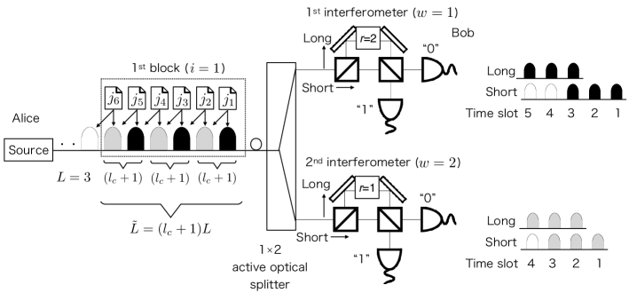
Figure 1: The setups of the source and the measurement devices under nearest-neighbor correlation ($l_{c}=1$), the number of pulses in each of the block to be fed into each of the interferometer $L$ being three ($L=3$), and block size being 6 ($\tilde{L}=(l_{c}+1)L=6$). For the $1^{{\rm st}}$ block ($i=1$), the positions of the black [gray] pulses belong to the $1^{{\rm st}}$ group ($w=1$), that is, $\mathcal{G}_{w=1}^{(1)}=\{1,3,5\}$ [$2^{{\rm nd}}$ group ($w=2$), that is, $\mathcal{G}_{w=2}^{(1)}=\{2,4,6\}$]. The black and gray pulses are respectively corresponds to $w=1$ and $w=2$, which are fed to the $1^{{\rm st}}$ and the $2^{{\rm nd}}$ variable-delay interferometer with two 50:50 beam splitters, respectively. Here, the delay $r$ is randomly chosen from the set $\{1,2\}$. The pulse trains from the interferometer are measured by two photon-number-resolving detectors representing bit values “0” and “1”. The successful detection in each of the interferometers occurs if Bob detects a single-photon in total among the $(r+1)^{{\rm th}}$ to the $L^{{\rm th}}$ time slots and observes no detection at the other time slots.

Before describing the protocol, we summarize the assumptions we make on the source and the receiver. Figure 1 depicts the setups of Alice and Bob’s devices employed in the protocol. Throughout the paper, we adopt the following notations. Let $N$ be the total number of pulses sent by Alice in the protocol, and for any symbol $A$, we define $\bm{A}_{i}:=A_{i},A_{i-1},...,A_{1}$ with $i\in\mathbb{N}$.

First, we list up the assumptions on Alice’s source as follows. As long as the following assumptions hold, any side-channel in the source can be accommodated.

1. For each $k^{{\rm th}}$ emitted pulse ($1\leq k\leq N$), Alice chooses a random bit $j_{k}\in\{0,1\}$. The bit $j_{k}$ is encoded not only to the $k^{{\rm th}}$ emitted pulse but also to the subsequence pulses. Let $l_{c}\geq 0$ be the number of pulses that the information $j_{k}$ is propagated, and we call $l_{c}$ correlation length. Let $|\psi_{j_{k}|j_{k-1},...,j_{1}}\rangle_{B_{k}}=|\psi_{j_{k}|\bm{j}_{k-1}}\rangle_{B_{k}}$ be the state of the $k^{{\rm th}}$ emitted signal to Bob, where the subscripts $j_{k-1},...,j_{1}$ indicate the dependency of the previous information $j_{k-1},...,j_{1}$. Note that $j_{0}$ represents having no condition. In defining the state $|\psi_{j_{k}|\bm{j}_{k-1}}\rangle_{B_{k}}$, we have the freedom in the choice of its global phase. Throughout this paper, we fix the global phase of the state $|\psi_{j_{k}|\bm{j}_{k-1}}\rangle_{B_{k}}$ such that the coefficient of the vacuum state is non-negative. In this paper, we consider the case where Alice employs $\tilde{L}$ pulses contained in a single-block, where $\tilde{L}$ is set to be $(l_{c}+1)L$ for $L\geq 3$. We call $\tilde{L}$ pulses of systems $B_{(i-1)\tilde{L}+1},...,B_{i\tilde{L}}$ the $i^{{\rm th}}$ block.

2. When $l_{c}\geq 1$, for any $k$ ($1\leq k\leq N$) and any $\zeta$ ($k+1\leq\zeta\leq\min\{N,k+l_{c}\})$, the following parameter $\epsilon_{\zeta-k}\geq 0$ characterizing the correlation is available.

   $$\left|\left\langle\psi_{j_{\zeta}|j_{\zeta-1},...,j_{k+1},j_{k}=1,\bm{j}_{k-1}}|\psi_{j_{\zeta}|j_{\zeta-1},...,j_{k+1},j_{k}=0,\bm{j}_{k-1}}\right\rangle\right|^{2}$$

   $$\geq 1-\epsilon_{\zeta-k}.$$ (1)

   Note that the difference between both states in the inner product is in the value of $j_{k}$. The parameter $\epsilon_{\zeta-k}$ depends only on the difference $\zeta-k$, but it is independent of $j_{\zeta},j_{\zeta-1},...,j_{k+1},j_{k-1},...,j_{1}$. Note that by the assumption (A1), if $\zeta\geq k+l_{c}+1$, the left hand size of Eq. (1) is equal to 1 since the bit information $j_{k}$ does not propagate to the $\zeta^{{\rm th}}$ state.

3. For any $k$ $(1\leq k\leq N)$ and any $j_{k}\in\{0,1\}$, the squared overlap of the vacuum state $|{\rm vac}\rangle$ and the state $|\psi_{j_{k}|j_{k-1},...,j_{1}}\rangle$ is lower-bounded by $p^{{\rm L}}_{{\rm vac},j_{k}}$ regardless of $k$ and the previous choices of $j_{k-1},...,j_{1}$. Mathematically, we suppose that

   $${\rm tr}\left[|{\rm vac}\rangle\langle{{\rm vac}}|\psi_{j_{k}|\bm{j}_{k-1}}\rangle\langle\psi_{j_{k}|\bm{j}_{k-1}}|\right]\geq p^{{\rm L}}_{{\rm vac},j_{k}}.$$ (2)

Providing the method for experimentally measuring the bounds in Eqs. (1) and (2) is beyond the scope of this paper. Note that the assumption (A2) can be alternatively expressed by using $p^{{\rm L}}_{{\rm vac},0}$ and $p^{{\rm L}}_{{\rm vac},1}$ in Eq. (2) because as we will show in Appendix A, the inner product in Eq. (1) can be lower-bounded as

$$\left|\left\langle\psi_{j_{\zeta}|j_{\zeta-1},...,j_{k+1},j_{k}=1,\bm{j}_{k-1}}|\psi_{j_{\zeta}|j_{\zeta-1},...,j_{k+1},j_{k}=0,\bm{j}_{k-1}}\right\rangle\right|$$

$$\geq\begin{cases}2p^{{\rm L}}_{{\rm vac},j_{\zeta}}-1&{\rm if}~{}2p^{{\rm L}}_{{\rm vac},j_{\zeta}}\geq 1\\ 0&{\rm otherwise}.\end{cases}$$ (3)

Next, we list up the assumptions on Bob’s measurement. As explained in Sec. II, we consider that Alice and Bob try to extract $(l_{c}+1)$ secret keys i.e., they divide each block into $(l_{c}+1)$ groups and try to generate a one bit key from each of the groups. In so doing, Bob employs $(l_{c}+1)$ variable-delay interferometers with $(L-1)$ delays followed by two detectors . To explain this more clearly, we classify the set $\{(i-1)\tilde{L}+1,(i-1)\tilde{L}+2,...,i\tilde{L}\}$ of the positions of the emitted pulses associated with the $i^{{\rm th}}$ block into $(l_{c}+1)$ groups, and the $w^{{\rm th}}$ group ($w\in\{1,2...,l_{c}+1\}$) for the $i^{{\rm th}}$ block is defined by

$$\mathcal{G}_{w}^{(i)}:=\{(l_{c}+1)(m-1)+w+(i-1)\tilde{L}\}_{m=1}^{L}.$$ (4)

Note that $w^{{\rm th}}$ group $\mathcal{G}_{w}^{(i)}$ is constructed by picking up all the $k^{{\rm th}}$ pulses from the $i^{{\rm th}}$ block with $k\equiv w$ in modulo $(l_{c}+1)$. For instance, if $i=1,l_{c}=2$, $L=10$ and $\tilde{L}=30$, $\mathcal{G}^{(1)}_{w=1}=\{1,4,7,...,28\},\mathcal{G}^{(1)}_{w=2}=\{2,5,8,...,29\}$ and $\mathcal{G}^{(1)}_{w=3}=\{3,6,9,...,30\}$. Then, Bob prepares $(l_{c}+1)$ interferometers, and for each $i^{{\rm th}}$ block, he feeds the incoming pulses of systems $\{B_{k}\}_{k\in\mathcal{G}_{w}^{(i)}}$ to the $w^{{\rm th}}$ interferometer.

1. Bob uses an active optical splitter with one-input and ($l_{c}+1$)-output to feed the pulses in the $i^{{\rm th}}$ block into the $(l_{c}+1)$ interferometers. This splitter actively sorts the incoming pulses to an appropriate interferometer, where the $k^{{\rm th}}$ pulse with $k\in\mathcal{G}_{w}^{(i)}$ is fed to the $w^{{\rm th}}$ interferometer.

2. Followed by the active optical splitter, Bob employs the $(l_{c}+1)$ variable-delay interferometers with two 50:50 beam splitters (BSs), where the delay of the interferometer is chosen uniformly at random from a set $\{1,2,...,L-1\}$. When $r$-bit delay ($r\in\{1,2,...,L-1\}$) is chosen in the interferometer, two pulses that are $r(l_{c}+1)$-pulses apart in terms of the pulses Alice emitted interfere.

3. After the interferometer, the pulses are detected at time slots 1 through $L+r$ by two photon-number-resolving (PNR) detectors, which discriminate the vacuum, a single-photon, and two or more photons of a specific optical mode. Each of the detectors is associated to bit values 0 and 1, respectively. We suppose that the quantum efficiencies and dark countings are the same for both detectors.

4. We suppose that there are no side-channels in Bob’s measurement device.

IV Protocol

In this section, we describe the actual protocol of the RRDPS protocol under the pulse correlations in the source device. Let $N_{{\rm em}}$ be the number of emitted blocks sent by Alice, and the total number of pulses sent by Alice is $N=N_{{\rm em}}\tilde{L}$. As we will see below, our protocol can be regarded as running $(l_{c}+1)$ RRDPS protocols simultaneously, each of which employs a block containing $L$ pulses. More specifically, our protocol runs as follows. In the description, $|\bm{z}|$ denotes the length of the bit sequence $\bm{z}$.

1. Alice and Bob respectively repeat steps 2 and 3 for $i=1,...,N_{{\rm em}}$.
   

2. Alice chooses a sequence of random bits $j_{(i-1)\tilde{L}+1},...,j_{i\tilde{L}}\in\{0,1\}^{\tilde{L}}$, and sends Bob the pulses in the following state through the quantum channel:

   $$\bigotimes_{k=(i-1)\tilde{L}+1}^{i\tilde{L}}|\psi_{j_{k}|j_{k-1},...,j_{1}}\rangle_{B_{k}}.$$ (5)

3. By the active optical splitter with one-input and ($l_{c}+1$)-output, the pulses in the $i^{{\rm th}}$ block are split to feed into the $(l_{c}+1)$ variable-delay interferometers. Among the pulses in the $i^{{\rm th}}$ block, the $k^{{\rm th}}$ pulse with $k\in\mathcal{G}_{w}^{(i)}$ is fed to the $w^{{\rm th}}$ interferometer.
   
   Bob executes the following for $w=1,...,l_{c}+1$.
   At the $w^{{\rm th}}$ interferometer, Bob randomly selects the delay $r\in\{1,2,...,L-1\}$, splits $L$ incoming pulses into two trains of pulses using a 50:50 BS, and shifts backwards only one of the two trains by $r$. Recall that the time of a single shift is equal to $(l_{c}+1)$-times as long as the interval of the neighboring emitted pulses. Then, Bob lets each of the first $L-r$ pulses in the shifted train interfere with each of the last $L-r$ pulses in the other train with the other 50:50 BS, and detects photons with the two PNR detectors at time slots 1 through $L+r$.

   1. When Bob detects exactly one photon among the $(r+1)^{{\rm th}}$ to the $L^{{\rm th}}$ time slots and observes no detection at the other time slots, he records a sifted key bit $z^{(w)}_{B,i}\in\{0,1\}$ depending on which detector reported the single photon. He also records the unordered pair $\{u^{(w)}_{i},v^{(w)}_{i}\}$, which are the positions of the pulse pair that resulted in the successful detection $(u^{(w)}_{i},v^{(w)}_{i}\in\{1,2,...,L\},|u^{(w)}_{i}-v^{(w)}_{i}|=r)$. He announces “success” and $\{u^{(w)}_{i},v^{(w)}_{i}\}$ over the classical channel.

   2. In all the cases other than (a), Bob announces “failure” and $w$ through the classical channel.

4. Bob executes the following for $w=1,...,l_{c}+1$.
   Let $N^{(w)}_{{\rm suc}}$ be the number of success blocks observed at the $w^{{\rm th}}$ interferometer. For these blocks, Bob defines his $w^{{\rm th}}$ type sifted key $\bm{z}^{(w)}_{B}$ by concatenating his sifted key bits $z^{(w)}_{B,i}$ for $i\in\mathcal{B}^{(w)}_{{\rm suc}}$. Here, the set $\mathcal{B}^{(w)}_{{\rm suc}}$ is composed of the block-index $i$ where the pulses whose indices in the set ${\mathcal{G}}^{(i)}_{w}$ result in the successful detection.

5. Alice executes the following for $w=1,...,l_{c}+1$.
   Alice calculates her sifted key bit $z^{(w)}_{A,i}=j_{k_{1}}\oplus j_{k_{2}}$ for $i\in\mathcal{B}^{(w)}_{{\rm suc}}$ with $k_{1}$ and $k_{2}$ being the $u^{(w)}_{i}$-th and the $v^{(w)}_{i}$-th elements of $\mathcal{G}_{w}^{(i)}$, and defines her $w^{{\rm th}}$ type sifted key $\bm{z}^{(w)}_{A}$ by concatenating her raw key bits $z^{(w)}_{A,i}$ for $i\in\mathcal{B}^{(w)}_{{\rm suc}}$.

6. Bob corrects the bit errors in $\bm{z}_{B}:=(\bm{z}^{(1)}_{B},...,\bm{z}^{(l_{c}+1)}_{B})$ to make it coincide with $\bm{z}_{A}:=(\bm{z}^{(1)}_{A},...,\bm{z}^{(l_{c}+1)}_{A})$ by sacrificing $|\bm{z}_{A}|f_{{\rm EC}}$ bits of encrypted public communication from Alice by consuming the same length of a pre-shared secret key.

7. Alice and Bob executes the following for $w=1,...,l_{c}+1$.
   For each $w^{{\rm th}}$ type reconciled key, Alice and Bob conduct privacy amplification by shortening their keys by $|\bm{z}^{(w)}_{A}|f^{(w)}_{{\rm PA}}$ to obtain the final keys.

In this paper, we only consider the secret key rate in the asymptotic limit of an infinite sifted key length. We consider the asymptotic limit of large $N_{{\rm em}}$ while the following observed parameters are fixed:

$$0\leq Q^{(w)}:=\frac{N^{(w)}_{{\rm suc}}}{N_{{\rm em}}}\leq 1.$$ (6)

Note that $f_{{\rm EC}}$ in step 6 is determined as a function of the bit error rate $e_{{\rm bit}}$ in $\bm{z}_{A}$ and $\bm{z}_{B}$, where $e_{{\rm bit}}$ can be estimated by random sampling whose cost is negligible in the asymptotic limit. Also, the fraction of privacy amplification $f^{(w)}_{{\rm PA}}$ in step 7 is determined by the experimentally available observables $Q^{(w)}$ in Eq. (6), $\{\epsilon_{d}\}_{d=1}^{l_{c}}$ in Eq. (1), $p^{{\rm L}}_{{\rm vac},0}$ and $p^{{\rm L}}_{{\rm vac},1}$ in Eq. (2), whose explicit form is given the next section.

V Security proof

V.1 Summary of security proof

Here, we summarize the result of the security proof of the protocol described above and determine the amount of privacy amplification $|\bm{z}^{(w)}_{A}|f^{(w)}_{{\rm PA}}$ for the $w^{{\rm th}}$ type sifted key in the asymptotic limit. As will be explained in this section, our security proof is based on the complementarity scenario koashi2009 in which estimation of an upper bound on the phase error rate assures the security. The main result is this upper bound, which is given in Theorem 1, and we provide its derivation in Sec. V.2. Here, we outline the crux of the discussions. The difficulty of our phase error rate estimation comes from the correlations among the emitted pulses that have not been accommodated in the previous security proofs of the RRDPS protocol  MIT2015 ; rr2016t ; rr2017t ; sasaki2017 ; rrt2017H ; rr2017tW ; Liu2017 ; Yin2018 ; Matsuura2019 . We solve this problem by exploiting the reference technique established in sciad . This is a technique that simplifies the estimation of the phase error rate when the actually employed states are close to the ones whose formula associated to the phase error rate is easily derived. In this technique, we consider reference states, which are fictitious states that are not prepared in the protocol but close to the actual state. The key intuition is rather simple; when the reference states and the actual states are close, the deviation between probabilities associated to the reference states and those associated to the actual states should not be large. Therefore, we can obtain the phase error rate formula for the actual states by slightly modifying the formula for the reference states. We emphasize that Alice does not need to generate the reference states in the protocol, and they are purely a mathematical tool for phase error rate estimation. In particular, we choose the reference states regarding the $k^{{\rm th}}$ emitted pulse such that the information $j_{k}$ is only encoded to system $B_{k}$ (see Eq. (31) for the explicit formula). By exploiting this property, it is simple to obtain the probabilities for the reference states, which will be given by $T$ in Eq. (26). Depending on the fidelity between the actual and reference states, which will be given by $S$ in Eq. (27), by slightly modifying the relationship for the reference states, we finally obtain the target probability with the actual ones.

In the rest of this section, we first explain the structure of the security proof, define the parameters that are needed to present the main result, and then describe Theorem 1. For the security proof with complementarity, we consider alternative entanglement-based procedures for Alice’s state preparation at step 2 and calculation of her raw key bit $z^{(w)}_{A,i}$ at step 5. These alternative procedures can be employed to prove the security of the actual protocol because the states sent to an eavesdropper (Eve), Bob’s measurement, and the final key are identical to those in the actual protocol. Also, Bob’s public announcement of the unordered pair $\{u^{(w)}_{i},v^{(w)}_{i}\}$ in the actual protocol is identical to the one in the alternative protocol. As for Alice’s state preparation at step 2, she alternatively prepares $N$ auxiliary qubits in systems $\bm{A}_{N}$, which remain at Alice’s laboratory during the whole protocol, and the $N$ pulses in systems $\bm{B}_{N}$ to be sent, in the following state

$$|\Psi\rangle_{\bm{A}_{N}\bm{B}_{N}}$$

$$:=\frac{1}{\sqrt{2^{N}}}\sum^{1}_{j_{N}=0}\cdots\sum^{1}_{j_{1}=0}\bigotimes_{k=1}^{N}|j_{k}\rangle_{A_{k}}e^{{\rm i}\theta_{j_{k}|\bm{j}_{k-1}}}|\psi_{j_{k}|\bm{j}_{k-1}}\rangle_{B_{k}}.$$ (7)

Here, the phase factors $e^{{\rm i}\theta_{j_{k}|\bm{j}_{k-1}}}$ can be chosen arbitrary because from Eve’s perspective, the states of system $B_{k}$ in Eqs. (5) and (7) are equivalent. However, these factors must be adequately chosen to apply the reference technique for each $w^{{\rm th}}$ type sifted key, which will be explained in Sec. V.2.2. As for calculation of the sifted key bit $z^{(w)}_{A,i}=j_{k_{1}}\oplus j_{k_{2}}$ at step 5, this bit can be alternatively extracted by applying the controlled-not (CNOT) gate (defined on the $Z$-basis) on the $k_{1}^{{\rm th}}$ and $k_{2}^{{\rm th}}$ auxiliary qubits of systems $A_{k_{1}}$ and $A_{k_{2}}$ with the $k_{1}^{{\rm th}}$ one being the control and the $k_{2}^{{\rm th}}$ one being the target followed by measuring the $k_{2}^{{\rm th}}$ auxiliary qubit in the $Z$-basis to obtain $z^{(w)}_{A,i}$.

In the complementarity scenario, the discussion of the security of the key $\bm{z}_{A}^{(w)}$ is equivalent to consider a virtual scenario of how well Alice can predict the outcome of the measurement complementary to the one to obtain $z_{A,i}^{(w)}$. In particular, we take the $X$-basis measurement as the complementary basis, and we need to quantify how well Alice can predict its outcome $x_{k_{2}}\in\{+,-\}$ on system $A_{k_{2}}$. As for Bob, instead of aiming at learning $z_{A,i}^{(w)}$, he performs the alternative measurement that determines which of the $k^{{\rm th}}$ pulse in the group $\mathcal{G}^{(i)}_{w}$ contains the single-photon. This measurement is complementary to the one for obtaining his sifted key bit $z_{B,i}^{(w)}$. With this alternative measurement, Bob announces the pair $\{u^{(w)}_{i},v^{(w)}_{i}\}$ such that the first index $u^{(w)}_{i}$ corresponds to the location of the single-photon and the second index $v^{(w)}_{i}$ is chosen uniformly at random from the set $\{1,2...,i-1,i+1,i+2...,L\}$ . Hence, in this virtual scenario, Alice’s task is to predict the outcome $x_{k_{2}}$ where $k_{2}$ is chosen uniformly at random from the group $\mathcal{G}^{(i)}_{w}$ except for $k_{1}$. We define the occurrence of phase error to be the case where Alice fails in her prediction of the outcome $x_{k_{2}}$. Let $N_{{\rm ph}}^{(w)}$ denote the number of phase errors of the $w^{{\rm th}}$ type sifted key among $|\bm{z}_{A}^{(w)}|$ trials. Suppose that the upper bound $N_{{\rm ph}}^{(w),{\rm U}}$ on $N_{{\rm ph}}^{(w)}$ is obtained as a function of the experimentally available observables $Q^{(w)}$ in Eq. (6), $\{\epsilon_{d}\}_{d=1}^{l_{c}}$ in Eq. (1), $p^{{\rm L}}_{{\rm vac},0}$ and $p^{{\rm L}}_{{\rm vac},1}$ in Eq. (2). In this case, in the asymptotic limit, a sufficient fraction of privacy amplification is given by koashi2009

$$f_{{\rm PA}}^{(w)}=h\left(N_{{\rm ph}}^{(w),{\rm U}}/N^{(w)}_{{\rm suc}}\right),$$ (8)

where $h(x)$ is defined by $h(x)=-x\log_{2}x-(1-x)\log_{2}(1-x)$ for $0\leq x\leq 0.5$ and $h(x)=1$ for $x>0.5$. Our main result, Theorem 1, derives the upper bound $e^{(w),{\rm U}}_{{\rm ph}}$ on the phase error rate $e^{(w)}_{{\rm ph}}:=N_{{\rm ph}}^{(w)}/N^{(w)}_{{\rm suc}}$ with $Q^{(w)}$, $\{\epsilon_{d}\}_{d=1}^{l_{c}}$, $p^{{\rm L}}_{{\rm vac},0}$ and $p^{{\rm L}}_{{\rm vac},1}$ (see Sec. V.2 for the proof).

Theorem 1

In the asymptotic limit of large key length of the $w^{{\rm th}}$ type sifted key $|\bm{z}^{(w)}_{A}|$, the upper bound on the phase error rate for the $w^{{\rm th}}$ type sifted key of the RRDPS protocol is given by

$$e^{(w),{\rm U}}_{{\rm ph}}=\sum_{s=0}^{L-2}\frac{1}{L-1}\min\left\{\frac{\nu(L,s,C)}{Q^{(w)}},1\right\}.$$ (9)

Here, function $\nu(L,s,C)$ is defined by

$$\nu(L,s,C):=\sum_{y=s+1}^{L}\binom{L}{y}C^{y}(1-C)^{L-y},$$

where $C=g(T,S)$ if $T\leq S^{2}$ and $C=1$ otherwise with $T:=1-\left(\sqrt{p_{{\rm vac},0}^{{\rm L}}}+\sqrt{p_{{\rm vac},1}^{{\rm L}}}\right)^{2}/4$, $S:=\left(1+\prod_{d=1}^{l_{c}}\sqrt{1-\epsilon_{d}}\right)/2$ for $l_{c}\geq 1$ and S=1 for $l_{c}=0$, and $g(x,y):=x+(1-y^{2})(1-2x)+2y\sqrt{(1-y^{2})x(1-x)}$.

We remark that once characterizations of the source device are completed (i.e., $\{\epsilon_{d}\}_{d=1}^{l_{c}}$, $p^{{\rm L}}_{{\rm vac},0}$ and $p^{{\rm L}}_{{\rm vac},1}$ are obtained), $C$ becomes a constant. Theorem 1 reveals that as the correlation length $l_{c}$ gets larger, $\nu(L,s,C)$ in the expression of the phase error rate in Eq. (9) generally gets larger because $C=g(T,S)$ is a monotonically decreasing function of $S$ and $S$ generally gets smaller as $l_{c}$ becomes larger.

Finally, using Theorem 1, the secret key rate per pulse is given by

$$R=\sum_{w=1}^{l_{c}+1}Q^{(w)}\left[1-f_{{\rm EC}}-h\left(e^{(w),{\rm U}}_{{\rm ph}}\right)\right]/(l_{c}+1)L,$$ (10)

where we provide its proof in Appendix C.

V.2 Proof of the main result

In this section, we prove our main result, Theorem 1.

V.2.1 Derivation of the phase error rate for the $w^{{\rm th}}$ type sifted key

Here, we derive the upper bound $e^{(w),{\rm U}}_{{\rm ph}}$ on the phase error rate $e^{(w)}_{{\rm ph}}:=N_{{\rm ph}}^{(w)}/N^{(w)}_{{\rm suc}}$ for the $w^{{\rm th}}$ type sifted key ($w\in\{1,2,...,l_{c}+1\}$). We remark that the following discussions hold for any $w$. To derive $e^{(w),{\rm U}}_{{\rm ph}}$, we consider performing the $X$-basis measurement on system $A_{k}$ of $|\Psi\rangle_{\bm{A}_{N}\bm{B}_{N}}$ in Eq. (7) with $k$ belonging to the $w^{{\rm th}}$ group of indices $\bigcup_{i=1}^{N_{{\rm em}}}\mathcal{G}^{(i)}_{w}$, and we define the total number of the minus $n_{w,-}^{(i)}$ with $1\leq i\leq N_{{\rm em}}$ obtained through measuring $L$ qubit systems $\{A_{k}\}_{k\in\mathcal{G}_{w}^{(i)}}$. Thanks to these $X$-basis measurements, we can classify $N^{(w)}_{{\rm suc}}$ successfully detected blocks according to $n_{w,-}$, which leads to $N^{(w)}_{{\rm ph}}=\sum_{s=0}^{L}N^{(w)}_{{\rm ph},n_{w,-}=s}$. Here, $N^{(w)}_{{\rm ph},n_{w,-}=s}$ denotes the number of the phase error events for the $w^{{\rm th}}$ type sifted key when $n_{w,-}=s$. By considering Bob’s alternative measurement explained in Sec. V.1, the probability of failing in the prediction of the $X$-basis measurement outcome (namely, having the occurrence of the phase error) when $n_{w,-}=s$ is $s/(L-1)$. More precisely, the phase error is defined by obtaining the outcome of the minus in the $X$-basis measurement on the target qubit, which is randomly chosen with probability $1/(L-1)$ rr . Since there are $s$-outcomes of the minus when $n_{w,-}=s$, the probability of obtaining the phase error is at most $s/(L-1)$. Importantly, the probability $1/(L-1)$ comes from the random choice of the delay at Bob’s measurement assumed in (B2), and Eve cannot distort this probability distribution rr . With this phase error probability $s/(L-1)$ when $n_{w,-}=s$, the Chernoff bound leads the following for any $\zeta>0$

$$e^{(w)}_{{\rm ph}} :=\frac{N_{{\rm ph}}^{(w)}}{N^{(w)}_{{\rm suc}}}=\frac{\sum_{s=0}^{L}N^{(w)}_{{\rm ph},n_{w,-}=s}}{N^{(w)}_{{\rm suc}}}$$

$$\leq\sum_{s=0}^{L-1}\frac{s}{L-1}\frac{N^{(w)}_{{\rm suc},n_{w,-}=s}}{N^{(w)}_{{\rm suc}}}+\zeta+\frac{N^{(w)}_{{\rm suc},n_{w,-}=L}}{N^{(w)}_{{\rm suc}}}$$

$$=\sum_{s=0}^{L-2}\frac{1}{L-1}\frac{N^{(w)}_{{\rm suc},n_{w,-}>s}}{N^{(w)}_{{\rm suc}}}+\zeta.$$ (11)

To upper-bound $N^{(w)}_{{\rm suc},n_{w,-}>s}/N^{(w)}_{{\rm suc}}$, whose trivial upper bound is 1, in addition to the successfully detected blocks, Alice measures the total number of the minus $n_{w,-}^{(i)}$ for the non-detected blocks (namely, all the $i^{\rm th}$ block with $i\notin\mathcal{B}^{(w)}_{{\rm suc}}$). In doing so, it is obvious to see that the number $N^{(w)}_{{\rm suc},n_{w,-}>s}$ of obtaining $n_{w,-}>s$ among the detected blocks can never be larger than the one $N^{(w)}_{{\rm em},n_{w,-}>s}$ among the emitted blocks . We note that the number $N^{(w)}_{{\rm em},n_{w,-}>s}$ of the emitted blocks is fixed once Alice prepares the state $|\Psi\rangle_{\bm{A}_{N}\bm{B}_{N}}$ in Eq. (7). By overestimating $N^{(w)}_{{\rm suc},n_{w,-}>s}$ as

$$N^{(w)}_{{\rm suc},n_{w,-}>s}\leq N^{(w)}_{{\rm em},n_{w,-}>s},$$ (12)

Eq. (11) results in

$$e^{(w)}_{{\rm ph}}\leq\sum_{s=0}^{L-2}\frac{1}{L-1}\min\left\{\frac{N^{(w)}_{{\rm em},n_{w,-}>s}}{N^{(w)}_{{\rm suc}}},1\right\}+\zeta.$$ (13)

Hence, the remaining task is to derive the upper bound on $N^{(w)}_{{\rm em},n_{w,-}>s}$. For this, we evaluate the upper bound on the probability of obtaining the outcome of the minus when system $A_{k}$ of state $|\Psi\rangle_{\bm{A}_{N}\bm{B}_{N}}$ is measured in the $X$-basis with $k$ belonging to the $m^{{\rm th}}$ element ($1\leq m\leq L$) of set $\mathcal{G}_{w}^{(i)}$. Mathematically, the target for computation is the probability ${\rm Pr}[x_{t}=-|\{x_{k}\}_{k\in\mathcal{P}^{(w)}_{i,m}}]$ with

$$t :=(i-1)\tilde{L}+w+(m-1)(l_{c}+1),$$

$$\mathcal{P}^{(w)}_{i,m} :=\bigcup_{a=1}^{i}\{k|k\in\mathcal{G}_{w}^{(a)},k<t\}.$$

If

$${\rm Pr}[x_{t}=-|\{x_{k}\}_{k\in\mathcal{P}^{(w)}_{i,m}},j_{t-1},...,j_{t-l_{c}}]\leq C$$ (14)

with constant $C$ holds for any $j_{t-1},...,j_{t-l_{c}}\in\{0,1\}^{l_{c}}$, where $j_{k}\in\{0,1\}$ denotes the $Z$-basis measurement outcome on system $A_{k}$ of Eq. (7), applying the Bayes rule leads that the target probability is also upper-bounded by $C$ :

$${\rm Pr}[x_{t}=-|\{x_{k}\}_{k\in\mathcal{P}^{(w)}_{i,m}}]\leq C.$$ (15)

The derivation of the upper-bound $C$ in Eq. (14) involves the reference technique established in sciad , and we explain its detail in Sec. V.2.2. Note that as mentioned in Sec. II, to apply the reference technique to estimate the statistics of $x_{t}$ in Eq. (14), the previous $l_{c}$ $Z$-basis measurement outcomes $j_{t-1},...,j_{t-l_{c}}$ must be fixed, where these $Z$-basis measurements are possible because we can discuss the security of each $w^{{\rm th}}$ type sifted key separately thanks to the modification of the RRDPS protocol. With Eq. (15) in hand, by considering the binomial trial with success probability $C$, the total number of the minus $n_{w,-}^{(i)}$ obtained through measuring $L$ systems $\{A_{k}\}_{k\in\mathcal{G}_{w}^{(i)}}$ obeys the following probability distribution when conditioned on the previous outcomes $n_{w,-}^{(i-1)},...,n_{w,-}^{(1)}$:

$${\rm Pr}[n_{w,-}^{(i)}>s|n_{w,-}^{(i-1)},...,n_{w,-}^{(1)}]\leq$$

$$\sum_{y=s+1}^{L}\binom{L}{y}C^{y}(1-C)^{L-y}=:\nu(L,s,C).$$ (16)

Here, $s$ denotes the integer. Once $s$ is fixed, $\nu(L,s,C)$ is constant independently of the block index $i$ $(1\leq i\leq N_{{\rm em}})$. Since the probability of obtaining $n_{w,-}>s$ for any $i^{{\rm th}}$ block is upper-bounded by $\nu(L,s,C)$ from Eq. (16), for deriving $N^{(w)}_{{\rm em},n_{w,-}>s}$, we can imagine independent trials with probability $\nu(L,s,C)$. Therefore, again by using the Chernoff bound, we have from Eq. (13) and $N^{(w)}_{{\rm em},n_{w,-}>s}/N^{(w)}_{{\rm suc}}=1/Q^{(w)}\cdot N^{(w)}_{{\rm em},n_{w,-}>s}/N_{{\rm em}}$ that for any $\chi>0$ and $\zeta>0$

$$e^{(w)}_{{\rm ph}}\leq\sum_{s=0}^{L-2}\frac{1}{L-1}\min\left\{\frac{\nu(L,s,C)+\chi}{Q^{(w)}},1\right\}+\zeta.$$ (17)

When we increase $N^{(w)}_{{\rm suc}}$ for any fixed $\zeta$ and $\chi$, the probability of violating Eq. (17) decreases exponentially. Therefore, in the limit of large $N^{(w)}_{{\rm suc}}$, we can neglect these terms and finally obtain our main result in Eq. (9). Note that $Q^{(w)}$ defined in Eq. (6) is experimentally observed data. As will be shown in Sec. V.2.2, $C$ is determined by the assumptions (A2) and (A3), namely, the parameters $\epsilon_{1},...,\epsilon_{l_{c}}$ in Eq. (1) and the probabilities $p^{{\rm L}}_{{\rm vac},0}$ and $p^{{\rm L}}_{{\rm vac},1}$ in Eq. (2).

V.2.2 Derivation of $X$-basis measurement statistics using reference technique

Here, we derive the upper bound on ${\rm Pr}[x_{t}=-|\{x_{k}\}_{k\in\mathcal{P}^{(w)}_{i,m}},j_{t-1},...,j_{t-l_{c}}]$ in Eq. (14), regardless of $j_{t-1},...,j_{t-l_{c}}\in\{0,1\}^{l_{c}}$ that are the $Z$-basis measurement outcomes of systems $A_{t-1},...,A_{t-l_{c}}$ in Eq. (7). The crucial point for its computation is that once $j_{t-1},...,j_{t-l_{c}}$ are fixed, we find from Eq. (7) that the state of the systems $\bm{A}_{t-1}\bm{B}_{t-1}$ and the one of the systems $\bm{A}_{\geq t}\bm{B}_{\geq t}$ are decoupled, i.e, they are in the tensor product. Here, we define $\bm{A}_{\geq i}:=A_{N},A_{N-1},...,A_{i}$. The $Z$-basis measurement outcomes $j_{t-1},...,j_{t-l_{c}}$ have an influence on determining the set of the $t^{{\rm th}}$ states $\{|\psi_{j_{t}|\bm{j}_{t-1}}\rangle_{B_{t}}\}_{j_{t}}$, but the previous $X$-basis measurement outcomes $\{x_{k}\}_{k\in\mathcal{P}^{(w)}_{i,m}}$ have no influence on the state of the systems $\bm{A}_{\geq t}\bm{B}_{\geq t}$ thanks to the tensor product structure. Therefore, when conditioned on $j_{t-1},...,j_{t-l_{c}}$, we only focus on the state of the systems $\bm{A}_{\geq t}\bm{B}_{\geq t}$ to calculate the target probability. From Eq. (7), conditioned on the outcomes $j_{t-1},...,j_{t-l_{c}}$, the state of systems $\bm{A}_{\geq t}\bm{B}_{\geq t}$ is written as

$$|\Gamma^{{\rm Act}}_{\bm{j}_{t-1}}\rangle_{\bm{A}_{\geq t}\bm{B}_{\geq t}}:=\frac{1}{\sqrt{2}}\sum_{j_{t}=0}^{1}|j_{t}\rangle_{A_{t}}|\psi^{{\rm Act}}_{j_{t}|\bm{j}_{t-1}}\rangle_{\bm{A}_{\geq t+1}\bm{B}_{\geq t}}$$ (18)

with

$$|\psi^{{\rm Act}}_{j_{t}|\bm{j}_{t-1}}\rangle_{\bm{A}_{\geq t+1}\bm{B}_{\geq t}}:=e^{{\rm i}\theta_{j_{t}|\bm{j}_{t-1}}}|\psi_{j_{t}|\bm{j}_{t-1}}\rangle_{B_{t}}\otimes$$

$$\frac{1}{\sqrt{2^{N-t}}}\sum_{j_{N}}\cdots\sum_{j_{t+1}}\bigotimes_{\zeta=t+1}^{N}|j_{\zeta}\rangle_{A_{\zeta}}e^{{\rm i}\theta_{j_{\zeta}|\bm{j}_{\zeta-1}}}|\psi_{j_{\zeta}|\bm{j}_{\zeta-1}}\rangle_{B_{\zeta}}.$$ (19)

As shown in sciad , and also in Appendix B, Eq. (19) is rewritten as

$$|\psi^{{\rm Act}}_{j_{t}|\bm{j}_{t-1}}\rangle_{\bm{A}_{\geq t+1}\bm{B}_{\geq t}}=e^{{\rm i}\theta_{j_{t}|\bm{j}_{t-1}}}|\psi_{j_{t}|\bm{j}_{t-1}}\rangle_{B_{t}}$$

$$\left[a_{j_{t},\bm{j}_{t-1}}|\Phi_{\bm{j}_{t-1}}\rangle_{\bm{A}_{\geq t+1}\bm{B}_{\geq t+1}}+b_{j_{t},\bm{j}_{t-1}}|\Phi^{\perp}_{j_{t},\bm{j}_{t-1}}\rangle_{\bm{A}_{\geq t+1}\bm{B}_{\geq t+1}}\right].$$ (20)

Here, $|\Phi_{\bm{j}_{t-1}}\rangle$ and $|\Phi^{\perp}_{j_{t},\bm{j}_{t-1}}\rangle$ are normalized states that respectively does not contain the information of $j_{t}$ and does contain its information. Note that the state $|\Phi_{\bm{j}_{t-1}}\rangle$ represents a side-channel-free state, while the state $|\Phi^{\perp}_{j_{t},\bm{j}_{t-1}}\rangle$ represents the state of the side-channel since the information of $j_{t}$ is propagated to the subsequence pulses. In our security proof, $|\Phi^{\perp}_{j_{t},\bm{j}_{t-1}}\rangle$ can be taken as any form in any-dimensional Hilbert space as long as it is orthogonal to $|\Phi_{\bm{j}_{t-1}}\rangle$, and the characterization of $|\Phi^{\perp}_{j_{t},\bm{j}_{t-1}}\rangle$ is not required. As stated below Eq. (7), the phase factors $e^{{\rm i}\theta_{j_{k}|\bm{j}_{k-1}}}$ in Eq. (7) can be chosen arbitrary, but to derive the lower bound on $a_{j_{t},\bm{j}_{t-1}}$ in Eq. (20), for each $k$ of $k\equiv w$ in modulo $l_{c}+1$, the phase factors $e^{{\rm i}\theta_{j_{k}|\bm{j}_{k-1}}}$ must be set as

$$e^{{\rm i}\theta_{j_{k}|\bm{j}_{k-1}}}=1,$$ (21)

and for each $k$ of $k\equiv w$ in modulo $l_{c}+1$, the phase factors $\{e^{{\rm i}\theta_{j_{\zeta}|\bm{j}_{\zeta-1}}}\}_{\zeta=k+1}^{k+l_{c}}$ must be chosen as

$$e^{{\rm i}\theta_{j_{\zeta}|\bm{j}_{\zeta-1}}}$$

$$:=\frac{\left|\left\langle\psi_{j_{\zeta}|j_{\zeta-1},...,j_{k+1},j_{k}=0,\bm{j}_{k-1}}|\psi_{j_{\zeta}|j_{\zeta-1},...,j_{k+1},j_{k},\bm{j}_{k-1}}\right\rangle\right|}{\left\langle\psi_{j_{\zeta}|j_{\zeta-1},...,j_{k+1},j_{k}=0,\bm{j}_{k-1}}|\psi_{j_{\zeta}|j_{\zeta-1},...,j_{k+1},j_{k},\bm{j}_{k-1}}\right\rangle}.$$ (22)

Note that $e^{{\rm i}\theta_{j_{t}|\bm{j}_{t-1}}}=1$ holds in Eqs. (19) and (20) because of Eq. (21) and $t\equiv w$ in modulo $l_{c}+1$. In doing so, the coefficient $a_{j_{t},\bm{j}_{t-1}}$ is positive and can be lower-bounded by using Eq. (1) as

$$a_{j_{t}=0,\bm{j}_{t-1}} =1,~{}~{}a_{j_{t}=1,\bm{j}_{t-1}}\geq\prod_{d=1}^{l_{c}}\sqrt{1-\epsilon_{d}}$$ (23)

if $l_{c}\geq 1$. If $l_{c}=0$, $a_{j_{t},\bm{j}_{t-1}}=1$ for both $j_{t}=0,1$ (see Appendix B for the detail).

Using Eq. (18), we have that the probability of our interest leads to

$${\rm Pr}[x_{t}=-|\{x_{k}\}_{k\in\mathcal{P}^{(w)}_{i,m}},j_{t-1},...,j_{t-l_{c}}]$$

$$={\rm tr}\left[|-\rangle\langle-|_{A_{t}}|\Gamma^{{\rm Act}}_{\bm{j}_{t-1}}\rangle\langle\Gamma^{{\rm Act}}_{\bm{j}_{t-1}}|_{\bm{A}_{\geq t}\bm{B}_{\geq t}}\right].$$ (24)

To calculate Eq. (24), we introduce the reference states $\{|\phi^{{\rm Ref}}_{j_{t}|\bm{j}_{t-1}}\rangle_{\bm{A}_{\geq t+1}\bm{B}_{\geq t}}\}_{j_{t}}$ that are associated with the actual states $\{|\psi^{{\rm Act}}_{j_{t}|\bm{j}_{t-1}}\rangle_{\bm{A}_{\geq t+1}\bm{B}_{\geq t}}\}_{j_{t}}$. The reference states, which are close to the actual states prepared by the protocol, need to be chosen such that the following two conditions are satisfied. In its description, we use the notation

$$|\Gamma^{{\rm Ref}}_{\bm{j}_{t-1}}\rangle_{\bm{A}_{\geq t}\bm{B}_{\geq t}}:=\frac{1}{\sqrt{2}}\sum_{j_{t}=0}^{1}|j_{t}\rangle_{A_{t}}|\phi^{{\rm Ref}}_{j_{t}|\bm{j}_{t-1}}\rangle_{\bm{A}_{\geq t+1}\bm{B}_{\geq t}}.$$ (25)

1. For the reference state, the probability of obtaining the outcome of the minus when system $A_{t}$ is measured in the $X$-basis is upper-bounded by constant $T>0$, which is expressed as

   $${\rm Pr}\left[x_{t}=-~{}|~{}|\Gamma^{{\rm Ref}}_{\bm{j}_{t-1}}\rangle\right]\leq T.$$ (26)

2. The fidelity between $|\Gamma^{{\rm Act}}_{\bm{j}_{t-1}}\rangle$ and $|\Gamma^{{\rm Ref}}_{\bm{j}_{t-1}}\rangle$ is lower-bounded by constant $S>0$, that is

   $$\left|\left\langle\Gamma^{{\rm Ref}}_{\bm{j}_{t-1}}|\Gamma^{{\rm Act}}_{\bm{j}_{t-1}}\right\rangle\right|\geq S.$$ (27)

Once the reference states satisfy Eqs. (26) and (27), the upper bound on Eq. (24) can be obtained by using the function $g(x,y)$ sciad that relates the statistics of the actual and the reference states . Specifically, the $X$-basis measurement statistics of these two states are related as

$${\rm Pr}\left[x_{t}=-~{}|~{}|\Gamma^{{\rm Act}}_{\bm{j}_{t-1}}\rangle\right]$$

$$\leq g\left({\rm Pr}\left[x_{t}=-~{}|~{}|\Gamma^{{\rm Ref}}_{\bm{j}_{t-1}}\rangle\right],\left|\left\langle\Gamma^{{\rm Ref}}_{\bm{j}_{t-1}}|\Gamma^{{\rm Act}}_{\bm{j}_{t-1}}\right\rangle\right|\right),$$ (28)

where $g(x,y)=x+(1-y^{2})(1-2x)+2y\sqrt{(1-y^{2})x(1-x)}$ if $x\leq y^{2}$ and $g(x,y)=1$ if $x>y^{2}$. A direct calculation reveals that if $x\leq y^{2}$,

$$g(x,y)\leq g(x^{{\rm U}},y^{{\rm L}})$$ (29)

holds, where U (L) indicates the upper (lower) bound. Then, combining Eqs. (26)-(29) gives

$${\rm Pr}\left[x_{t}=-~{}|~{}|\Gamma^{{\rm Act}}_{\bm{j}_{t-1}}\rangle\right]\leq C=\begin{cases}g(T,S)&({\rm if}~{}T\leq S^{2})\\ 1&({\rm if}~{}T>S^{2}).\end{cases}$$ (30)

Hence, the remaining task for obtaining Eq. (15) is to derive the two bounds $T$ and $S$, which are calculated below. In so doing, we take the reference state $|\phi^{{\rm Ref}}_{j_{t}|\bm{j}_{t-1}}\rangle_{\bm{A}_{\geq t+1}\bm{B}_{\geq t}}$ for $j_{t}\in\{0,1\}$, which are associated with the actual state $|\psi^{{\rm Act}}_{j_{t}|\bm{j}_{t-1}}\rangle_{\bm{A}_{\geq t+1}\bm{B}_{\geq t}}$ in Eq. (20), such that it is the first term of $|\psi^{{\rm Act}}_{j_{t}|\bm{j}_{t-1}}\rangle_{\bm{A}_{\geq t+1}\bm{B}_{\geq t}}$:

$$|\phi^{{\rm Ref}}_{j_{t}|\bm{j}_{t-1}}\rangle_{\bm{A}_{\geq t+1}\bm{B}_{\geq t}}=|\psi_{j_{t}|\bm{j}_{t-1}}\rangle_{B_{t}}\otimes|\Phi_{\bm{j}_{t-1}}\rangle_{\bm{A}_{\geq t+1}\bm{B}_{\geq t+1}}.$$ (31)

Calculation of $T$ in Eq. (26):
We calculate the upper bound on ${\rm Pr}\left[x_{t}=-~{}|~{}|\Gamma^{{\rm Ref}}_{\bm{j}_{t-1}}\rangle\right]$ as follows:

$${\rm Pr}\left[x_{t}=-~{}|~{}|\Gamma^{{\rm Ref}}_{\bm{j}_{t-1}}\rangle\right]=1-{\rm Pr}\left[x_{t}=+~{}|~{}|\Gamma^{{\rm Ref}}_{\bm{j}_{t-1}}\rangle\right]$$

$$=1-\sum_{n=0}^{\infty}{\rm Pr}\left[n_{t}=n,x_{t}=+~{}|~{}|\Gamma^{{\rm Ref}}_{\bm{j}_{t-1}}\rangle\right]$$

$$\leq 1-{\rm Pr}\left[n_{t}=0,x_{t}=+~{}|~{}|\Gamma^{{\rm Ref}}_{\bm{j}_{t-1}}\rangle\right],$$

where $n_{t}$ denotes the number of photons contained in system $B_{t}$. By rewriting $|\Gamma^{{\rm Ref}}_{\bm{j}_{t-1}}\rangle$ using the $X$-basis states $|\pm\rangle_{A_{t}}$:

$$|\Gamma^{{\rm Ref}}_{\bm{j}_{t-1}}\rangle_{\bm{A}_{\geq t}\bm{B}_{\geq t}}=|\Phi_{\bm{j}_{t-1}}\rangle_{\bm{A}_{\geq t+1}\bm{B}_{\geq t+1}}\otimes$$

$$\frac{|+\rangle_{A_{t}}\sum_{j_{t}}|\psi_{j_{t}|\bm{j}_{t-1}}\rangle_{B_{t}}+|-\rangle_{A_{t}}\sum_{j_{t}}(-1)^{j_{t}}|\psi_{j_{t}|\bm{j}_{t-1}}\rangle_{B_{t}}}{2},$$ (32)

we find that the statistics of $n_{t}$ only depends on system $A_{t}$. Importantly, in obtaining Eq. (32), we used the fact that $|\Phi_{\bm{j}_{t-1}}\rangle_{\bm{A}_{\geq t+1}\bm{B}_{\geq t+1}}$ is independent of $j_{t}$ as stated in Sec. V.2.2. Then, combining Eq. (32) and the assumption (A3) in Sec. III gives the lower-bound on ${\rm Pr}\left[n_{t}=0,x_{t}=+~{}|~{}|\Gamma^{{\rm Ref}}_{\bm{j}_{t-1}}\rangle\right]$ as

$${\rm Pr}\left[n_{t}=0,x_{t}=+~{}|~{}|\Gamma^{{\rm Ref}}_{\bm{j}_{t-1}}\rangle\right]=\left|\frac{\langle{\rm vac}|\sum_{j_{t}}|\psi_{j_{t}|\bm{j}_{t-1}}\rangle}{2}\right|^{2}$$

$$\geq\left[\sqrt{p_{{\rm vac},0}^{{\rm L}}}+\sqrt{p_{{\rm vac},1}^{{\rm L}}}\right]^{2}/4.$$

In the inequality, we employ the fact that the coefficient of the vacuum state of $|\psi_{j_{t}|\bm{j}_{t-1}}\rangle$ is non-negative, which is stated in assumption (A1). Therefore,

$${\rm Pr}\left[x_{t}=-~{}|~{}|\Gamma^{{\rm Ref}}_{\bm{j}_{t-1}}\rangle\right]\leq 1-\left(\sqrt{p_{{\rm vac},0}^{{\rm L}}}+\sqrt{p_{{\rm vac},1}^{{\rm L}}}\right)^{2}/4=T.$$

Calculation of $S$ in Eq. (27):
Next, we calculate the fidelity between $|\Gamma^{{\rm Act}}_{\bm{j}_{t-1}}\rangle$ and $|\Gamma^{{\rm Ref}}_{\bm{j}_{t-1}}\rangle$. We have that for $l_{c}\geq 1$

$$\left|\left\langle\Gamma^{{\rm Ref}}_{\bm{j}_{t-1}}|\Gamma^{{\rm Act}}_{\bm{j}_{t-1}}\right\rangle\right|=\frac{\left|\sum_{j_{t}}\left\langle\phi^{{\rm Ref}}_{j_{t}|\bm{j}_{t-1}}|\psi^{{\rm Act}}_{j_{t}|\bm{j}_{t-1}}\right\rangle\right|}{2}$$

$$=\frac{\left|\sum_{j_{t}}a_{j_{t},\bm{j}_{t-1}}\right|}{2}\geq\frac{1+\prod_{d=1}^{l_{c}}\sqrt{1-\epsilon_{d}}}{2}=S.$$

The first equality follows from Eqs. (18) and (25), the second equality comes from Eqs. (20) and (31), and the inequality follows from Eq. (23). If $l_{c}=0$, $S=1$ holds since $a_{j_{t},\bm{j}_{t-1}}=1$ for both $j_{t}=0,1$.

VI Simulation of secure key rates

Figure 2: Secure key rate $R$ per pulse as a function of the overall channel transmission $\eta$. From top to bottom, we plot the key rates for $(l_{c},\Delta)=$(0,0), (1,0.2), (2,0.2) and (10,0.2) with $e_{{\rm bit}}=3\%$ and $L=32$. We note that the key rates for the last three parameters are almost superposed.

Here, we show the simulation results of asymptotic key rate $R$ per pulse given by Eq. (10) as a function of the overall channel transmission $\eta$ including the detector efficiency. For the simulation, we assume that each emitted pulse is a coherent pulse from a conventional laser with mean photon number $\mu$ and only the phases of the coherent pulses are correlated. In this case, the lower bound on the vacuum emission probability $p^{{\rm L}}_{{\rm vac},j_{k}}$ in Eq. (2) is given by $e^{-\mu}$ and hence $T$ defined above is $1-e^{-\mu}$. For the simulation, we consider the cases of the correlation length $l_{c}=0,1,2$ and 10, and for all the cases, we adopt $f_{{\rm EC}}=h(e_{{\rm bit}})$ with $e_{{\rm bit}}$ denoting the bit error rate in the protocol and suppose the successful detection rate for any $w$ as $Q^{(w)}=L\eta\mu e^{-L\eta\mu}/2$.

In the case of $l_{c}=1$, namely, the case of the nearest-neighbor correlation, we assume that the $k^{{\rm th}}$ emitted state is written as

$$|\psi_{j_{k}|j_{k-1}}\rangle=\delta_{j_{k-1},0}|(-1)^{j_{k}}\sqrt{\mu}\rangle+\delta_{j_{k-1},1}|(-1)^{j_{k}}\sqrt{\mu}e^{{\rm i}\Delta}\rangle.$$ (33)

Here, $\delta_{x,y}$ is the Kronecker delta and $|e^{{\rm i}\theta}\sqrt{\mu}\rangle$ denotes the coherent state with the complex amplitude being $e^{{\rm i}\theta}\sqrt{\mu}$. This state represents the pulse correlation that if the previous choice of bit $j_{k-1}$ is 0, then the next $k^{{\rm th}}$ states are the ideal states $\{|\sqrt{\mu}\rangle,|-\sqrt{\mu}\rangle\}$, but if $j_{k-1}$ is 1, then the phases are deviated by $\Delta$ from the ideal ones. In this setting, $S$ defined above is given by

$$S=\frac{1+\sqrt{1-\epsilon_{1}}}{2}=\frac{1+|\left\langle\sqrt{\mu}|\sqrt{\mu}e^{{\rm i}\Delta}\right\rangle|}{2}=\frac{1+e^{\mu(\cos\Delta-1)}}{2}.$$

In the case of $l_{c}=2$, we assume that the $k^{{\rm th}}$ emitted state is written as $|\psi_{j_{k}|j_{k-1},j_{k-2}}\rangle=\delta_{j_{k-1},0}\delta_{j_{k-2},0}|(-1)^{j_{k}}\sqrt{\mu}\rangle+\delta_{j_{k-1},0}\delta_{j_{k-2},1}|(-1)^{j_{k}}\sqrt{\mu}e^{{\rm i}\Delta/2}\rangle+\delta_{j_{k-1},1}\delta_{j_{k-2},0}|(-1)^{j_{k}}\sqrt{\mu}e^{{\rm i}\Delta}\rangle+\delta_{j_{k-1},1}\delta_{j_{k-2},1}|(-1)^{j_{k}}\sqrt{\mu}e^{{\rm i}3\Delta/2}\rangle$. This state represents that if $j_{k-1}=1$ ($j_{k-2}=1$), the phases of the $k^{{\rm th}}$ pulses are rotated by $\Delta$ ($\Delta/2$). This means that the influence of the second-previous bit $j_{k-2}$ to the $k^{{\rm th}}$ pulse is half of that of the previous bit $j_{k-1}$. In this setting, $S$ is given by

$$S=\frac{1+\sqrt{1-\epsilon_{1}}\sqrt{1-\epsilon_{2}}}{2}=\frac{1+e^{\mu(\cos\Delta-1)}e^{\mu(\cos\frac{\Delta}{2}-1)}}{2}.$$

As for the case of $l_{c}=10$, the $k^{{\rm th}}$ state is set to be analogous to the one for $l_{c}=1,2$, where if $j_{k-d}=1$ (with $d=1,...,10$), the phases of the $k^{{\rm th}}$ pulses are rotated by $\Delta/2^{d-1}$. A direct calculation shows $S=\left(1+\prod_{d=1}^{10}\sqrt{1-\epsilon_{d}}\right)/2=\left(1+\prod_{d=1}^{10}e^{\mu(\cos(\Delta/2^{d-1})-1)}\right)/2.$

In Fig. 2, we plot the key rates for $e_{{\rm bit}}=0.03$, $L=32$ and $\Delta=0.2$ rad for the cases of $l_{c}=0,1,2,10$ from top to bottom. The top line is the key rate with no pulse correlation (i.e., $l_{c}=0$) that corresponds to $\Delta=0$ in Eq. (33). The key rates are optimized over mean photon number $\mu$ for each value of channel transmission $\eta$. From these lines, we see that the pulse correlation slightly degrades the key rate (about 0.7 times lower than the one without pulse correlation), but the three lines with $l_{c}=1,2$ and 10 are almost superposed. This implies that when the pulse correlation gets weaker as the pulses are farther apart, which is assumed in our simulation, the long-range pulse correlation does not cause a significant impact on the key rate.

VII Discussion

In this paper, we have provided the information theoretic security proof of the RRDPS protocol with the pulse correlation in Alice’s source by using the reference technique. The pulse correlation is one of the serious imperfections in high-speed QKD systems where Alice’s random bit choice is propagated to the subsequent emitted pulses. Once the number of propagated pulses ($l_{c}$) is fixed, our security proof only requires the two experimentally simple assumptions on the source: the lower bound on the fidelity between the two $k^{{\rm th}}$ states when the correlation patterns are different and the lower bounds on the vacuum emission probabilities of each emitted pulse. Our numerical simulations have shown the key rates up to $l_{c}=10$ and have revealed that the long-range pulse correlation does not cause a significant impact on the key rate in a realistic experimental setting. Therefore, our security proof is effective and applicable to wide range of practical sources, and thus paves the way to realize the truly secure and high-speed QKD systems.

We end with some open questions. It has an practical importance to simulate the key rates based on another source correlation model such as an intensity correlation that is beyond the one we have supposed in our simulation shown in Fig. 2. Also, it is interesting to extend our security proof without the modification of the protocol, namely, with a single variable-delay interferometer assuming the same source correlation. Another interesting topic is to extend the security proof to accommodate quantum correlations among the emitted signals.

Appendix A Proof of Eq. (3)

In this appendix, we prove Eq. (3). For this, once we obtain the following proposition, by substituting $|\psi\rangle=|\psi_{j_{\zeta}|j_{\zeta-1},...,j_{k+1},j_{k}=1,j_{k-1},...,j_{1}}\rangle$, $|\phi\rangle=|\psi_{j_{\zeta}|j_{\zeta-1},...,j_{k+1},j_{k}=0,j_{k-1},...,j_{1}}\rangle$ and the lower bounds in Eq. (2) to Eq. (34), Eq. (3) can be obtained.

Proposition 1

For any state $|\psi\rangle$ and $|\phi\rangle$, a lower bound on the fidelity between these two states is given by

$$|\left\langle\psi|\phi\right\rangle|\geq\begin{cases}2\sqrt{p_{{\rm vac},\phi}p_{{\rm vac},\psi}}-1&{\rm if}~{}2\sqrt{p_{{\rm vac},\phi}p_{{\rm vac},\psi}}\geq 1\\ 0&{\rm otherwise},\end{cases}$$ (34)

where $p_{{\rm vac},\phi}:={\rm tr}[|{\rm vac}\rangle\langle{\rm vac}||\phi\rangle\langle\phi|]$.

(Proof) We expand $|\psi\rangle$ and $|\phi\rangle$ using the photon number states in all the optical modes, $|{\rm vac}\rangle$ and $\{|n\rangle\}_{n\geq 1}$, as follows:

$$|\psi\rangle =\sqrt{p_{{\rm vac},\psi}}|{\rm vac}\rangle+\sum_{n\geq 1}\beta_{n}|n\rangle,$$

$$|\phi\rangle =\sqrt{p_{{\rm vac},\phi}}|{\rm vac}\rangle+\sum_{n\geq 1}\gamma_{n}|n\rangle.$$

We here choose the global phase of $|\psi\rangle$ and $|\phi\rangle$ such that the coefficients of $|{\rm vac}\rangle$ being positive, and $\beta_{n}\in\mathbb{C}$ and $\gamma_{n}\in\mathbb{C}$ are the coefficients for $n\geq 1$ of $|\psi\rangle$ and $|\phi\rangle$, respectively. By using this, $|\left\langle\psi|\phi\right\rangle|$ is written as

$$|\left\langle\psi|\phi\right\rangle|=\left|\sqrt{p_{{\rm vac},\psi}p_{{\rm vac},\phi}}+e^{{\rm i}\theta}\left|\sum_{n\geq 1}\beta_{n}^{\ast}\gamma_{n}\right|\right|,$$ (35)

where $\theta=\arg(\sum_{n\geq 1}\beta_{n}^{\ast}\gamma_{n})$. We next derive the upper bound on $\left|\sum_{n\geq 1}\beta_{n}^{\ast}\gamma_{n}\right|$ by exploiting the triangle inequality and the Cauchy-Schwarz inequality:

$$\left|\sum_{n\geq 1}\beta_{n}^{\ast}\gamma_{n}\right| \leq\sum_{n\geq 1}\left|\beta_{n}\right|\left|\gamma_{n}\right|\leq\sqrt{\left(\sum_{n\geq 1}|\beta_{n}|^{2}\right)\left(\sum_{n\geq 1}|\gamma_{n}|^{2}\right)}$$

$$=\sqrt{(1-p_{{\rm vac},\psi})(1-p_{{\rm vac},\phi})}=:\tau.$$

1. If $2\sqrt{p_{{\rm vac},\phi}p_{{\rm vac},\psi}}\geq 1$, since $\sqrt{p_{{\rm vac},\phi}p_{{\rm vac},\psi}}\geq\tau$ holds, Eq. (35) is lower-bounded as follows:

   $$|\left\langle\psi|\phi\right\rangle|$$

   $$\geq \left|\sqrt{p_{{\rm vac},\phi}p_{{\rm vac},\psi}}+e^{{\rm i}\pi}\tau\right|$$

   $$= \sqrt{p_{{\rm vac},\phi}p_{{\rm vac},\psi}}-\sqrt{(1-p_{{\rm vac},\psi})(1-p_{{\rm vac},\phi})}$$

   $$\geq \sqrt{p_{{\rm vac},\phi}p_{{\rm vac},\psi}}-\sqrt{1+p_{{\rm vac},\psi}p_{{\rm vac},\phi}-2\sqrt{p_{{\rm vac},\phi}p_{{\rm vac},\psi}}}$$

   $$= 2\sqrt{p_{{\rm vac},\phi}p_{{\rm vac},\psi}}-1.$$

   The second inequality follows from the fact that $a+b\geq 2\sqrt{ab}$ holds for any $a,b\geq 0$.

2. If $2\sqrt{p_{{\rm vac},\phi}p_{{\rm vac},\psi}}<1$, we only have the trivial lower bound:

   $$|\left\langle\psi|\phi\right\rangle|\geq 0.$$ (36)

Appendix B Proof of Eqs. (20) and (23)

In this appendix, we prove Eqs. (20) and (23). We start form Eq. (19):

$$|\psi^{{\rm Act}}_{j_{t}|\bm{j}_{t-1}}\rangle_{\bm{A}_{\geq t+1}\bm{B}_{\geq t}}=e^{{\rm i}\theta_{j_{t}|\bm{j}_{t-1}}}|\psi_{j_{t}|\bm{j}_{t-1}}\rangle_{B_{t}}\left(\frac{1}{\sqrt{2^{N-t}}}\sum_{j_{N}}\cdots\sum_{j_{t+1}}\bigotimes_{\zeta=t+1}^{N}|j_{\zeta}\rangle_{A_{\zeta}}e^{{\rm i}\theta_{j_{\zeta}|\bm{j}_{\zeta-1}}}|\psi_{j_{\zeta}|j_{\zeta-1},...,j_{t+1},j_{t},\bm{j}_{t-1}}\rangle_{B_{\zeta}}\right).$$ (37)

To see how the information $j_{t}$ is encoded to the state $|\psi^{{\rm Act}}_{j_{t}|\bm{j}_{t-1}}\rangle_{\bm{A}_{\geq t+1}\bm{B}_{\geq t}}$, we expand it using $|\Phi_{\bm{j}_{t-1}}\rangle_{\bm{A}_{\geq t+1}\bm{B}_{\geq t+1}}$ and $|\Phi^{\perp}_{j_{t},\bm{j}_{t-1}}\rangle_{\bm{A}_{\geq t+1}\bm{B}_{\geq t+1}}$ to have

$$|\psi^{{\rm Act}}_{j_{t}|\bm{j}_{t-1}}\rangle_{\bm{A}_{\geq t+1}\bm{B}_{\geq t}}=e^{{\rm i}\theta_{j_{t}|\bm{j}_{t-1}}}|\psi_{j_{t}|\bm{j}_{t-1}}\rangle_{B_{t}}\otimes$$

$$\left(a_{j_{t},\bm{j}_{t-1}}|\Phi_{\bm{j}_{t-1}}\rangle_{\bm{A}_{\geq t+1}\bm{B}_{\geq t+1}}+b_{j_{t},\bm{j}_{t-1}}|\Phi^{\perp}_{j_{t},\bm{j}_{t-1}}\rangle_{\bm{A}_{\geq t+1}\bm{B}_{\geq t+1}}\right),$$ (38)

where $|\Phi_{\bm{j}_{t-1}}\rangle_{\bm{A}_{\geq t+1}\bm{B}_{\geq t+1}}$ and $|\Phi^{\perp}_{j_{t},\bm{j}_{t-1}}\rangle_{\bm{A}_{\geq t+1}\bm{B}_{\geq t+1}}$ denote some normalized states, and these are orthogonal each other. The subscripts in $a_{j_{t},\bm{j}_{t-1}}$, $b_{j_{t},\bm{j}_{t-1}}$, $|\Phi_{\bm{j}_{t-1}}\rangle_{\bm{A}_{\geq t+1}\bm{B}_{\geq t+1}}$, and $|\Phi^{\perp}_{j_{t},\bm{j}_{t-1}}\rangle_{\bm{A}_{\geq t+1}\bm{B}_{\geq t+1}}$ indicate the dependency on the previous setting choices . Importantly, $|\Phi_{\bm{j}_{t-1}}\rangle_{\bm{A}_{\geq t+1}\bm{B}_{\geq t+1}}$ does not depend on $j_{t}$ but $|\Phi^{\perp}_{j_{t},\bm{j}_{t-1}}\rangle_{\bm{A}_{\geq t+1}\bm{B}_{\geq t+1}}$ does. This means that $|\Phi^{\perp}_{j_{t},\bm{j}_{t-1}}\rangle_{\bm{A}_{\geq t+1}\bm{B}_{\geq t+1}}$ represents the side-channel state of $j_{t}$. For $|\Phi_{\bm{j}_{t-1}}\rangle_{\bm{A}_{\geq t+1}\bm{B}_{\geq t+1}}$, we can take any state as long as it is independent of $j_{t}$. Here, we choose it as

$$|\Phi_{\bm{j}_{t-1}}\rangle_{\bm{A}_{\geq t+1}\bm{B}_{\geq t+1}}=\frac{1}{\sqrt{2^{N-t}}} \left(\sum_{j_{t+l_{c}}}\cdots\sum_{j_{t+1}}\bigotimes_{\zeta=t+1}^{t+l_{c}}|j_{\zeta}\rangle_{A_{\zeta}}|\psi_{j_{\zeta}|j_{\zeta-1},...,j_{t+1},j_{t}=0,\bm{j}_{t-1}}\rangle_{B_{\zeta}}\right)$$

$$\otimes \left(\sum_{j_{N}}\cdots\sum_{j_{t+l_{c}+1}}\bigotimes_{\zeta=t+l_{c}+1}^{N}e^{{\rm i}\theta_{j_{\zeta}|\bm{j}_{\zeta-1}}}|j_{\zeta}\rangle_{A_{\zeta}}|\psi_{j_{\zeta}|j_{\zeta-1},...,j_{t+1},j_{t}=0,\bm{j}_{t-1}}\rangle_{B_{\zeta}}\right)$$ (39)

that corresponds to the $N-t$ systems of Eq. (37) with $j_{t}$ being fixed to be 0 and with omitting the phase from the state $\{|\psi_{j_{\zeta}|j_{\zeta-1},...,j_{t+1},j_{t}=0,\bm{j}_{t-1}}\rangle_{B_{\zeta}}\}_{\zeta=t+1}^{t+l_{c}}$. The reason for omitting the phase is to guarantee the positivity of $a_{j_{t},\bm{j}_{t-1}}$ in Eq. (38). The remaining task is to derive the lower bound on $a_{j_{t},\bm{j}_{t-1}}$ for $j_{t}\in\{0,1\}$ using the assumption (A2). Since $a_{j_{t},\bm{j}_{t-1}}$ is the inner product between Eq. (39) and the vector

$$\frac{1}{\sqrt{2^{N-t}}}\sum_{j_{N}}\cdots\sum_{j_{t+1}}$$

$$\bigotimes_{\zeta=t+1}^{N}|j_{\zeta}\rangle_{A_{\zeta}}e^{{\rm i}\theta_{j_{\zeta}|\bm{j}_{\zeta-1}}}|\psi_{j_{\zeta}|j_{\zeta-1},...,j_{t+1},j_{t},\bm{j}_{t-1}}\rangle_{B_{\zeta}},$$

which is the state of the $N-t$ systems shown in the parenthesis of Eq. (37), we have

$$a_{j_{t},\bm{j}_{t-1}} =\frac{1}{2^{N-t}}\left(\sum_{j_{t+l_{c}}}\cdots\sum_{j_{t+1}}\prod_{\zeta=t+1}^{t+l_{c}}e^{{\rm i}\theta_{j_{\zeta}|\bm{j}_{\zeta-1}}}\left\langle\psi_{j_{\zeta}|j_{\zeta-1},...,j_{t+1},j_{t}=0,\bm{j}_{t-1}}|\psi_{j_{\zeta}|j_{\zeta-1},...,j_{t+1},j_{t},\bm{j}_{t-1}}\right\rangle\right)\left(\sum_{j_{N}}\cdots\sum_{j_{t+l_{c}+1}}1\right)$$

$$=\frac{1}{2^{l_{c}}}\sum_{j_{t+l_{c}}}\cdots\sum_{j_{t+1}}\prod_{\zeta=t+1}^{t+l_{c}}e^{{\rm i}\theta_{j_{\zeta}|\bm{j}_{\zeta-1}}}\left\langle\psi_{j_{\zeta}|j_{\zeta-1},...,j_{t+1},j_{t}=0,\bm{j}_{t-1}}|\psi_{j_{\zeta}|j_{\zeta-1},...,j_{t+1},j_{t},\bm{j}_{t-1}}\right\rangle$$

$$=\frac{1}{2^{l_{c}}}\sum_{j_{t+l_{c}}}\cdots\sum_{j_{t+1}}\prod_{\zeta=t+1}^{t+l_{c}}\left|\left\langle\psi_{j_{\zeta}|j_{\zeta-1},...,j_{t+1},j_{t}=0,\bm{j}_{t-1}}|\psi_{j_{\zeta}|j_{\zeta-1},...,j_{t+1},j_{t},\bm{j}_{t-1}}\right\rangle\right|.$$ (40)

In the second equality, we set the phases $e^{{\rm i}\theta_{j_{\zeta}|\bm{j}_{\zeta-1}}}$ for any $\zeta$ ($t+1\leq\zeta\leq t+l_{c}$) and $\bm{j}_{N}$ as

$$e^{{\rm i}\theta_{j_{\zeta}|\bm{j}_{\zeta-1}}}$$

$$:=\frac{\left|\left\langle\psi_{j_{\zeta}|j_{\zeta-1},...,j_{t+1},j_{t}=0,\bm{j}_{t-1}}|\psi_{j_{\zeta}|j_{\zeta-1},...,j_{t+1},j_{t},\bm{j}_{t-1}}\right\rangle\right|}{\left\langle\psi_{j_{\zeta}|j_{\zeta-1},...,j_{t+1},j_{t}=0,\bm{j}_{t-1}}|\psi_{j_{\zeta}|j_{\zeta-1},...,j_{t+1},j_{t},\bm{j}_{t-1}}\right\rangle}.$$ (41)

Since the only difference between both states in the inner product of Eq. (40) is in the $j_{t}^{{\rm th}}$ index, we have

$$a_{j_{t}=0,\bm{j}_{t-1}}=1.$$

On the other hand, if $j_{t}=1$, by applying Eq. (1) to Eq. (40), we obtain

$$a_{j_{t}=1,\bm{j}_{t-1}} \geq\frac{1}{2^{l_{c}}}\sum_{j_{t+l_{c}}}\cdots\sum_{j_{t+1}}\prod_{\zeta=t+1}^{t+l_{c}}\sqrt{1-\epsilon_{\zeta-t}}$$

$$=\prod_{d=1}^{l_{c}}\sqrt{1-\epsilon_{d}}.$$

This ends the proof of Eqs. (20) and (23).   $\blacksquare$

Appendix C Proof of Eq. (10)

In this appendix, we prove Eq. (10) that is our result of the security proof. Our security proof adopts the composability definition composable , where the security of our RRDPS protocol is evaluated by the correctness and secrecy parameters. As shown in koashi2009 , these parameters can be quantified separately, and since the correctness parameter is obtained by a verification step of the protocol, our target is to compute the secrecy parameter $\epsilon_{s}$. The protocol is $\epsilon_{s}$-secret if and only if

$$d:=||\rho^{{\rm final}}_{\bm{A}_{{\rm final}}E}-\rho^{{\rm ideal}}_{\bm{A}_{{\rm final}}E}||\leq\epsilon_{s}.$$ (42)

Here, we define trace distance $||X||:={\rm tr}[\sqrt{X^{\dagger}X}]/2$, $\rho^{{\rm final}}_{\bm{A}_{{\rm final}}E}$ denotes the state of Alice’s actual final keys and Eve’s quantum system, and $\rho^{{\rm ideal}}_{\bm{A}_{{\rm final}}E}$ denotes the state of ideal final keys that are completely secret from Eve and Eve’s quantum system. These final keys can be obtained by applying a quantum circuit (composed of a lot of CNOT gates), which is determined by random matrices used in privacy amplification. We introduce a quantum operation $\mathcal{E}^{(w)}_{{\rm act}}$ that extracts the $w^{{\rm th}}$-type final key from $w^{{\rm th}}$-type sifted qubits of systems $\bm{A}_{{\rm sift}}^{(w)}$. The operation $\mathcal{E}^{(w)}_{{\rm act}}$ is composed of CNOT gates acting on systems $\bm{A}^{(w)}_{{\rm sift}}$ and $Z$-basis measurements. The total operation in privacy amplification to obtain the final keys, which acts on all the sifted qubits of systems $\bm{A}_{{\rm sift}}:=\bm{A}^{(1)}_{{\rm sift}}\bm{A}^{(2)}_{{\rm sift}}...\bm{A}^{(l_{c}+1)}_{{\rm sift}}$, is then written as

$$\mathcal{E}_{{\rm act}}:=\bigotimes_{w=1}^{l_{c}+1}\mathcal{E}^{(w)}_{{\rm act}}.$$ (43)

Using this definition, $\rho^{{\rm final}}_{\bm{A}_{{\rm final}}E}$ and $\rho^{{\rm ideal}}_{\bm{A}_{{\rm final}}E}$ in Eq. (42) can be written as

$$\rho^{{\rm final}}_{\bm{A}_{{\rm final}}E}=\mathcal{E}_{{\rm act}}(\rho_{\bm{A}_{{\rm sift}}E}),$$ (44)

$$\rho^{{\rm ideal}}_{\bm{A}_{{\rm final}}E}=\mathcal{E}_{{\rm act}}(|\bm{+}\rangle\langle\bm{+}|_{\bm{A}_{{\rm sift}}}\otimes{\rm tr}_{\bm{A}_{{\rm sift}}}[\rho_{\bm{A}_{{\rm sift}}E}]),$$ (45)

where $\rho_{\bm{A}_{{\rm sift}}E}$ is the state of Alice’s all the sifted qubits and Eve’s quantum system just before executing privacy amplification $\mathcal{E}_{{\rm act}}$. Note that $|+\rangle:=(|0\rangle+|1\rangle)/\sqrt{2}$ is the $X$-basis eigenstate from which an ideal key can be extracted. We use the notation $|\bm{+}\rangle_{\bm{A}_{{\rm sift}}}$ to express all the qubits of systems $\bm{A}_{{\rm sift}}$ being in $|+\rangle$. Below, we show that the above trace distance $d$ can be upper-bounded by using our Theorem 1. In this theorem, as we consider the asymptotic limit of an infinite sifted key length, we neglect the probability of failing in obtaining the upper bound of Eq. (9). For a general discussion here, we denote its negligible probability of failing in obtaining Eq. (9) for $w$ by $\xi^{(w)}$. With these failure probabilities and Theorem 1, we have the following proposition.

Proposition 2

When Eq. (9) in our Theorem 1 holds except for probability $\xi^{(w)}$, and if the amount of privacy amplification applied for the $w^{{\rm th}}$-type reconciled key is set to be

$$N^{(w)}_{{\rm suc}}h(e^{(w),{\rm U}}_{{\rm ph}})+\log_{2}\frac{1}{\eta^{(w)}}$$ (46)

for any $\eta^{(w)}>0$, the secrecy parameter $\epsilon_{s}$ of the RRDPS protocol is given by

$$\epsilon_{s}=\sum_{w=1}^{l_{c}+1}\sqrt{2}\sqrt{\xi^{(w)}+\eta^{(w)}}.$$ (47)

Here, $h(x)$ denotes the binary entropy function, and $N^{(w)}_{{\rm suc}}$ is the number of sifted qubits of systems $\bm{A}^{(w)}_{{\rm sift}}$.

In the asymptotic limit ($N^{(w)}_{{\rm suc}}\to\infty$), as $\xi^{(w)}\to 0$ and $\eta^{(w)}\to 0$, $\epsilon_{s}$ in Eq. (47) results in negligible. Therefore, using this proposition by setting $\xi^{(w)}\to 0$ and $\eta^{(w)}\to 0$, we finally obtain the secret key rate shown in Eq. (10) with $\epsilon_{s}$-secret. The rest of this appendix is devoted to proving this proposition.

(Proof) First, when the amount of privacy amplification is set to be as Eq. (46), it is straightforward from HayashiNaka to derive the secrecy parameter for the $w^{{\rm th}}$-type key, that is, we obtain for any $w\in\{1,2,...,l_{c}+1\}$,

$$||\mathcal{E}^{(\geq w)}_{{\rm act}}({\rm tr}_{\bm{A}^{(0,...,w-1)}_{{\rm sift}}}[\rho_{\bm{A}_{{\rm sift}}E}])$$

$$-\mathcal{E}^{(\geq w)}_{{\rm act}}(|\bm{+}\rangle\langle\bm{+}|_{\bm{A}^{(w)}_{{\rm sift}}}\otimes{\rm tr}_{\bm{A}^{(1,...,w)}_{{\rm sift}}}[\rho_{\bm{A}_{{\rm sift}}E}])||$$

$$\leq\sqrt{2}\sqrt{\xi^{(w)}+\eta^{(w)}}=:\Delta^{(w)}.$$ (48)

Here, we define $\mathcal{E}^{(\geq w)}_{{\rm act}}:=\bigotimes_{x=w}^{l_{c}+1}\mathcal{E}^{(x)}_{{\rm act}}$ and ${\rm tr}_{\bm{A}^{(0)}_{{\rm sift}}}$ means that no system is traced out. This bound $\Delta^{(w)}$ is obtained by executing phase error correction to correct all the qubits of systems $\bm{A}^{(w)}_{{\rm sift}}$ to $|+\rangle$. This operation of its correction does not change any statistics of the measurement outcomes obtained by $\mathcal{E}^{(\geq w)}_{{\rm act}}$, and hence we can insert this operation to upper-bound the trace distance in Eq. (48). Then, based on HayashiNaka , this trace distance can be evaluated by the failure probability $\eta^{(w)}$ of phase error correction when $e^{(w),{\rm U}}_{{\rm ph}}$ is obtained and the failure probability $\xi^{(w)}$ of obtaining the upper-bound on the phase error rate $e^{(w),{\rm U}}_{{\rm ph}}$. We remark that in doing this argument of phase error correction, the state $\rho_{\bm{A}_{{\rm sift}}E}$ must be dependent on $w\in\{1,2,...,l_{c}+1\}$. This is because we define the virtual state $|\Psi\rangle_{\bm{A}_{N}\bm{B}_{N}}$ in Eq. (7) for each $w$ differently (due to the phase factors $e^{{\rm i}\theta_{j_{k}|\bm{j}_{k-1}}}$ defined in Eqs. (21) and (22)) in order to obtain the upper bound on the phase error rate for each $w$, which is explained in Sec. V.2.2. The differences of the states $\rho_{\bm{A}_{{\rm sift}}E}$ for $w$ become apparent in correcting the phase errors for each $w^{{\rm th}}$-type sifted qubits. Importantly, however, these differences do not change any statistics of the final keys obtained through the operation $\mathcal{E}_{{\rm act}}$ . Therefore, we can take the state $\rho_{\bm{A}_{{\rm sift}}E}$ independently of $w$ when we consider the security of the final keys in Eq. (48). This is the reason why the state $\rho_{\bm{A}_{{\rm sift}}E}$ in Eq. (48) does not depend on $w$.

Then, by exploiting Eq. (48) and substituting Eqs. (44) and (45) to Eq. (42), $d$ is calculated as follows:

$$d \leq||\mathcal{E}_{{\rm act}}(\rho_{\bm{A}_{{\rm sift}}E})-\mathcal{E}_{{\rm act}}(|\bm{+}\rangle\langle\bm{+}|_{\bm{A}^{(w=1)}_{{\rm sift}}}\otimes{\rm tr}_{\bm{A}^{(w=1)}_{\rm sift}}[\rho_{\bm{A}_{\rm sift}E}])||$$

$$+||\mathcal{E}_{{\rm act}}(|\bm{+}\rangle\langle\bm{+}|_{\bm{A}^{(w=1)}_{{\rm sift}}}\otimes{\rm tr}_{\bm{A}^{(w=1)}_{\rm sift}}[\rho_{\bm{A}_{\rm sift}E}])-\mathcal{E}_{{\rm act}}(|\bm{+}\rangle\langle\bm{+}|_{\bm{A}_{{\rm sift}}}\otimes{\rm tr}_{\bm{A}_{{\rm sift}}}[\rho_{\bm{A}_{{\rm sift}}E}])||$$ (49)

$$\leq\Delta^{(1)}+||\mathcal{E}^{(\geq 2)}_{{\rm act}}({\rm tr}_{\bm{A}^{(w=1)}_{\rm sift}}[\rho_{\bm{A}_{\rm sift}E}])-\mathcal{E}^{(\geq 2)}_{{\rm act}}(|\bm{+}\rangle\langle\bm{+}|_{\bm{A}^{(w\geq 2)}_{{\rm sift}}}\otimes{\rm tr}_{\bm{A}_{{\rm sift}}}[\rho_{\bm{A}_{{\rm sift}}E}])||$$ (50)

$$\leq\Delta^{(1)}+||\mathcal{E}^{(\geq 2)}_{{\rm act}}({\rm tr}_{\bm{A}^{(w=1)}_{\rm sift}}[\rho_{\bm{A}_{\rm sift}E}])-\mathcal{E}^{(\geq 2)}_{{\rm act}}(|\bm{+}\rangle\langle\bm{+}|_{\bm{A}^{(w=2)}_{{\rm sift}}}\otimes{\rm tr}_{\bm{A}^{(w=1,2)}_{{\rm sift}}}[\rho_{\bm{A}_{{\rm sift}}E}])||$$

$$+||\mathcal{E}^{(\geq 2)}_{{\rm act}}(|\bm{+}\rangle\langle\bm{+}|_{\bm{A}^{(w=2)}_{{\rm sift}}}\otimes{\rm tr}_{\bm{A}^{(w=1,2)}_{{\rm sift}}}[\rho_{\bm{A}_{{\rm sift}}E}])-\mathcal{E}^{(\geq 2)}_{{\rm act}}(|\bm{+}\rangle\langle\bm{+}|_{\bm{A}^{(w\geq 2)}_{{\rm sift}}}\otimes{\rm tr}_{\bm{A}_{{\rm sift}}}[\rho_{\bm{A}_{{\rm sift}}E}])||$$ (51)

$$\leq\Delta^{(1)}+\Delta^{(2)}+||\mathcal{E}^{(\geq 2)}_{{\rm act}}(|\bm{+}\rangle\langle\bm{+}|_{\bm{A}^{(w=2)}_{{\rm sift}}}\otimes{\rm tr}_{\bm{A}^{(w=1,2)}_{{\rm sift}}}[\rho_{\bm{A}_{{\rm sift}}E}])-\mathcal{E}^{(\geq 2)}_{{\rm act}}(|\bm{+}\rangle\langle\bm{+}|_{\bm{A}^{(w\geq 2)}_{{\rm sift}}}\otimes{\rm tr}_{\bm{A}_{{\rm sift}}}[\rho_{\bm{A}_{{\rm sift}}E}])||.$$ (52)

The first and third inequalities come from the triangle inequality of trace distance, and the second and fourth ones follow from Eq. (48). So far, we have quantified the security of the $w^{{\rm th}}$-type keys for $w=1,2$. By repeating the same arguments for $w=3,4,...,l_{c}$, we have

$$d\leq\sum_{w=1}^{l_{c}}\Delta^{(w)}+||\mathcal{E}^{(\geq l_{c}+1)}_{{\rm act}}({\rm tr}_{\bm{A}^{(w=1,2...,l_{c})}_{\rm sift}}[\rho_{\bm{A}_{\rm sift}E}])-\mathcal{E}^{(\geq l_{c}+1)}_{{\rm act}}(|\bm{+}\rangle\langle\bm{+}|_{\bm{A}^{(w=l_{c}+1)}_{{\rm sift}}}\otimes{\rm tr}_{\bm{A}_{{\rm sift}}}[\rho_{\bm{A}_{{\rm sift}}E}])||.$$ (53)

Finally, applying Eq. (48) for $w=l_{c}+1$, we obtain

$$d \leq\sum_{w=1}^{l_{c}+1}\Delta^{(w)},$$ (54)

which ends the proof.   $\blacksquare$

References

- (1) H.-K. Lo, M. Curty, and K. Tamaki, Nature Photonics 8, 595 (2014).
- (2) K. Yoshino, M. Fujiwara, K. Nakata, T. Sumiya, T. Sasaki, M. Takeoka, M. Sasaki, A. Tajima, M. Koashi, and A. Tomita, npj Quantum Information 4, 8 (2018).
- (3) E. Diamanti, H.-K. Lo, B. Qi, and Z. Yuan, npj Quantum Information 2, 16025 (2016).
- (4) V. Zapatero, A. Navarrete, K. Tamaki, and M. Curty, arXiv:2105.11165v1 (2021).
- (5) M. Pereira, G. Kato, A. Mizutani, M. Curty, and K. Tamaki, Science Advances 6, eaaz4487 (2020).
- (6) A. Mizutani, G. Kato, K. Azuma, M. Curty, R. Ikuta, T. Yamamoto, N. Imoto, H. K. Lo, and K. Tamaki, npj Quantum Information 5, 8 (2019).
- (7) T. Sasaki, Y. Yamamoto, and M. Koashi, Nature 509, 475 (2014).
- (8) A. Mizutani, N. Imoto, and K. Tamaki, Phys. Rev. A 92, 060303 (2015).
- (9) H.-L. Yin, Y. Fu, Y. Mao, and Z.-B. Chen, Phys. Rev. A 93, 022330 (2016).
- (10) Z. Zhang, X. Yuan, Z. Cao, and X. Ma, New Journal of Physics 19, 033013 (2017).
- (11) T. Sasaki and M. Koashi, Quantum Science and Technology 2, 024006 (2017).
- (12) Y. Hatakeyama, A. Mizutani, G. Kato, N. Imoto, and K. Tamaki, Phys. Rev. A 95, 042301 (2017).
- (13) L. Wang and S. Zhao, Quantum Information Processing 16, 100 (2017).
- (14) L. Liu, F.-Z. Guo, S.-J. Qin, and Q.-Y. Wen, Scientific Reports 7, 42261 (2017).
- (15) Z.-Q. Yin, S. Wang, W. Chen, Y.-G. Han, R. Wang, G.-C. Guo, and Z.-F. Han, Nature Communications 9, 457 (2018).
- (16) T. Matsuura, T. Sasaki, and M. Koashi, Phys. Rev. A 99, 042303 (2019).
- (17) H. Takesue, T. Sasaki, K. Tamaki, and M. Koashi, Nature Photonics 9, 827 (2015).
- (18) S. Wang, Z.-Q. Yin, W. Chen, D.-Y. He, X.-T. Song, H.- W. Li, L.-J. Zhang, Z. Zhou, G.-C. Guo, and Z.-F. Han, Nature Photonics 9, 832 (2015).
- (19) J.-Y. Guan, Z. Cao, Y. Liu, G.-L. Shen-Tu, J. S. Pelc, M. M. Fejer, C.-Z. Peng, X. Ma, Q. Zhang, and J.-W. Pan, Phys. Rev. Lett. 114, 180502 (2015).
- (20) Y.-H. Li, Y. Cao, H. Dai, J. Lin, Z. Zhang, W. Chen, Y. Xu, J.-Y. Guan, S.-K. Liao, J. Yin, et al., Phys. Rev. A 93, 030302 (2016).
- (21) F. Bouchard, A. Sit, K. Heshami, R. Fickler, and E. Karimi, Phys. Rev. A 98, 010301 (2018).
- (22) M. Koashi, New Journal of Physics 11, 045018 (2009).
- (23) M. Ben-Or, M. Horodecki, D. W. Leung, D. Mayes, and J. Oppenheim, Second Theory of Cryptography Conf. TCC (Lecture Notes in Computer Science vol 3378) (Berlin: Springer) pp 386-406 (2005).
- (24) A. Mizutani, T. Sasaki, Y. Takeuchi, K. Tamaki, and M. Koashi, npj Quantum Information 5, 87 (2019).
- (25) M. Hayashi, R. Nakayama, New Journal of Physics 16, 063009 (2014).