Inverting elastic dislocations using the
Weakly-enforced Slip Method

1 Introduction

With the advent of satellite based interferometry, or InSAR, routine measurements of the earth’s surface deformation have become available, providing a wealth of information about subsurface processes [1]. One of these processes is tectonic faulting, along with its violent manifestation, earthquakes. While the dynamics of the quake itself cannot be measured from space in the way that seismometers do, what can be measured to great accuracy is the lasting adjustments of static equilibrium to the defect that results from the relative displacement, or slip, of two adjacent masses along a fault.

Given two measurements of the earth’s surface covering the area of an earthquake, of which one taken just prior, the other just after, it can be reasonably assumed that the differences can be wholly attributed to the process of tectonic faulting [14]. Separation of co-seismic and post-seismic signal can be controlled by shortening the satellite revisit time [3]. However, to establish the details of the faulting mechanism that corresponds to the observed co-seismic deformation, such as the location and orientation of the fault, and the amount, depth and direction of the slip that occurred, we require an understanding of the physics bridging the two.

It is generally assumed that on the near-instantaneous time scale of co-seismic deformation, the earth behaves to a good approximation elastically [16]. The default model connecting the fault mechanism and surface observations, therefore, is that of static, elastic dislocations. While a formal definition of this problem will be presented in Section 2, sufficing at present is that this type of problem has been studied for well over a century, during which a range of solution methods has been devised of which [19] provide an overview.

Of the many solution methods available, the most powerful is arguably the finite element method [24], which is capable of incorporating all available knowledge of material heterogeneity and surface topography and thus capturing the system to the greatest detail. Regrettably, for reasons of computational cost, InSAR analyses are commonly performed on the other end of the complexity spectrum, in the confines of a homogeneous half space for which analytical expressions are available — see, for example  [17, 4, 22]. It is with this situation in mind that [20] proposed the Weakly-enforced Slip Method (WSM), in an attempt to combine the power of the finite element method with the computational efficiency of analytical expressions.

The efficiency of WSM does come at a price: the displacement field it produces is continuous, and therefore unable to capture the jump at the fault. In [20] it was however shown that the error thus incurred decays exponentially with distance to the fault. It was therefore hypothesized that this drawback is of little consequence in the context of satellite observations, as most surface measurements are sufficiently far removed from the dislocation. Only rupturing or near-rupturing faults will cause numerical errors that significantly interfere with the observables, and even that only locally. As InSAR data tends to be of low quality in these regions with damage leading to decorrelation, it is hoped that a reduction of numerical accuracy in this region will be of little consequence.

It bears repeating that the above considerations are speculative. While [20] proved the mathematical soundness of the WSM, it is in the present paper that we set out to thoroughly test the utility of the WSM in the problem setting for which it was devised. To this end a number of synthetic but otherwise fully representative case studies are presented and analysed using the WSM, as well as validated against the exact solutions. For the sake of this validation the scenarios will be restricted to homogeneous half spaces so that exact solutions are available in the form of analytical expressions, but it is to be understood that the presented methodology is valid for the wider class of problems including material heterogeneity and topography.

The central problem that is studied in this paper is the following:

(Inverse problem) Given observed displacements of the earth’s surface, determine the fault location and slip distribution that are in best accordance with these observations, as well as an uncertainly measure for this result.

To solve this problem we first need to address the conjugate question:

(Forward problem) Given a fault location and slip distribution, determine the surface displacements that we can expect to observe.

The forward problem is the topic of Section 2, the inverse problem that of Section 3. Section 4 will define the methodology and introduce case studies, and Section 5 will present the results of the comparative study.

2 Forward Problem: Linear Elastic Dislocation

To formally define the dislocation problem that will stand model to the earth’s response to tectonic faulting, we will denote by $\Omega$ the solid domain, by $d$ its spatial dimension, and by $u:\Omega\rightarrow\mathbb{R}^{d}$ the deformation field, i.e. the displacement of the solid compared to its reference configuration. We assume that it is possible to create a mapping from the deformation field $u$ to the corresponding state of internal stress $\sigma$. In particular, we assume that the stress depends linearly on the deformation gradient, leading to the well known constitutive relation

$$\sigma(u)=C:\nabla u,$$ (1)

where $C:\Omega\rightarrow\mathbb{R}^{d\times d\times d\times d}$ is the stiffness tensor representing local material properties. For the medium to be at rest, Newton’s second law states that the divergence of stress must be in balance with the applied loading. Rather than incorporating the loading conditions of the earth’s gravitational field, we use the linearity of the stress-strain relation of Equation (1) to have $u$ represent only the deviations relative to the existing equilibrium. The earth’s gravitational field being constant in time, this means the stress field (1) is divergence free.

Through the remainder of this document we will use a consistent notation for the four spaces that form the basis of our mathematical framework. By $\mathcal{X}$ we denote the space of local fault plane coordinates $\xi\in\mathbb{R}^{d-1}$. By $\mathcal{M}$ we denote the space of all possible fault geometries $m:\mathcal{X}\rightarrow\mathbb{R}^{d}$ that position the manifold in physical space. By $\mathcal{B}$ we denote the space of slip distributions pulled back to $\mathcal{X}$, the slip vector $b(\xi)$ being the jump in the displacement field when passing from one side of the manifold to the other. By $\mathcal{D}$ we denote the space of surface displacements $d:\mathbb{R}^{d-1}\rightarrow\mathbb{R}$ as measured in line of sight to the satellite. With this notation in place we can reformulate the forward problem as follows:

(Forward problem) Determine the surface observations $d\in\mathcal{D}$ corresponding to a given manifold $m\in\mathcal{M}$ and slip distribution $b\in\mathcal{B}$.

We denote the fault plane $\mathcal{F}$ and the domain boundary $\Gamma$ as shown in Figure 1. At the fault $\mathcal{F}=m(\mathcal{X})$ we demand that the displacement field $u$ jumps discontinuously by a distance $b$. Since this makes the displacement field locally non-differentiable, the stress is locally not defined, and our general equilibrium condition does not apply. Instead, Newton’s second law transforms into a jump condition for the traction, stating that the tractions on either side of the fault plane must be in balance. At the earth’s surface $\Gamma_{\rm surf}$ we assume traction-free conditions, and the remaining domain boundary $\Gamma_{\rm far}$ is assumed to be sufficiently far away for the relative displacements to be zero. Taken together, this results in the following system of equations for the forward problem:

$$\left\{\begin{array}[]{r@{\ }l@{\text{ at }}l}\mathrm{div}\,\sigma(u)&=0&\Omega\setminus\mathcal{F}\text{ (static equilibrium, continuum)}\\ {}[\![u]\!]&=b\circ m^{-1}&\mathcal{F}\text{ (fault slip)}\\ {}[\![\sigma(u)]\!]\nu&=0&\mathcal{F}\text{ (static equilibrium across fault)}\\ \sigma(u)n&=0&\Gamma_{\rm surf}\text{ (traction-free surface)}\\ u&=0&\Gamma_{\rm far}\text{ (zero displacement at far field)}\\ \end{array}\right.$$ (2)

Figure 1: Adapted from [19], visualization of the forward problem and all entities of Equation (2).

Before looking into solution strategies for this system, it is readily apparent that solutions to this problem are linear in $b$. Hence, for any manifold $m\in\mathcal{M}$, there exists a linear map from the space of slip distributions to the corresponding observations:

$$F_{m}:\mathcal{B}\rightarrow\mathcal{D}.$$ (3)

If $\mathcal{B}$ and $\mathcal{D}$ are finite-dimensional and endowed with a basis, we can identify every linear operator with a matrix, $F_{m}\in\mathbb{R}^{\#\mathcal{B}\times\#\mathcal{D}}$, where $\#(\cdot)$ denotes the cardinality of set $(\cdot)$.

2.1 Analytical solutions

The general expression for solutions to (2) was presented in integral form by Volterra [21]:

$$u_{n}(y)=\sum_{ijkl}\int_{\xi\in\mathcal{X}}b_{i}(\xi)\nu_{j}(\xi)C_{ijkl}(m(\xi))\frac{\partial u_{k}^{n}}{\partial x_{l}}(m(\xi),y)\det\left|\frac{\partial m}{\partial\xi}\right|d\xi,$$ (4)

where the Green’s function $u_{k}^{n}(x,y)$ is the $k$-th component of the displacement vector in $x$ due to a unit point force at $y$ in direction $n$. Note that (4) has an equivalent alternative form owing to the symmetry relation $u_{k}^{n}(x,y)=u_{n}^{k}(y,x)$, which is a direct result of Betti’s reciprocal theorem [9].

To obtain closed form expressions for the Green’s function we need to place additional constraints on our system. Firstly, we require that the elastic properties of our medium are homogeneous and isotropic, thus reducing the constitutive model to having two independent parameters. Choosing as our parameters the Young’s modulus $E$ and Poisson’s ratio $\nu$, the constitutive tensor becomes

$$C_{ijkl}=\frac{E}{2+2\nu}\left[\frac{2\nu}{1-2\nu}\delta_{ij}\delta_{kl}+\delta_{ik}\delta_{jl}+\delta_{il}\delta_{jk}\right].$$ (5)

Since the displacement resulting from a unit force is inversely proportional to the Young’s modulus, we observe that the displacement field resulting from Volterra’s equation (4) depends only on the Poisson’s ratio of the medium.

Secondly, for closed form expressions for the Green’s functions $u^{k}_{n}(x,p)$ to be available, we require the physical domain $\Omega$ to be a half space, that is, to have an infinite, flat surface as its free surface $\Gamma_{\rm surf}$ and the far field boundary $\Gamma_{\rm far}$ at infinity. The Green’s functions for the 2D half space were derived by Melan [11], those for the 3D half space by Mindlin [12].

Building on Mindlin’s results, closed form expressions for Volerra’s equation have been presented by Yoffe [23] and Okada [13], subject to further restrictions in terms of fault planes and slip distributions. While it is these results that are typically used in practical applications, for the purposes of our study we shall apply Volterra’s equation directly so as not to incur additional and unnecessary restrictions to our case studies that would diminish the value of the present study.

2.2 The Weakly-enforced Slip Method

The Weakly-enforced Slip Method is a special case of the Finite Element Method, which is in turn a Galerkin method, employing shape functions to construct a finite system of equations that can be solved numerically. Contrary to classical finite element treatments of Equation (2), in which the domain must be discretized such that the mesh conforms to the manifold $m$, the defining property of the Weakly-enforced Slip Method is that the finite element mesh can be formed independent of $m$.

Foregoing derivations and proofs, which are presented in detail in [20], we present the WSM only in terms of its core result. Given a finite element discretization for the computational domain $\Omega$ with mesh density $h$, and generating from it a discrete, vector-valued function space $\hat{V}$, the WSM solution to Equation (2) is the field $\hat{u}\in\hat{V}$ that satisfies, for all test functions $\hat{v}\in\hat{V}$,

$$\int_{\Omega}\nabla\hat{u}:C:\nabla\hat{v}=\sum_{ijkl}\int_{\xi\in\mathcal{X}}b_{i}(\xi)\nu_{j}(\xi)\left\{C_{ijkl}(m(\xi))\frac{\partial\hat{v}_{k}}{\partial x_{l}}(m(\xi))\right\}\det\left|\frac{\partial m}{\partial\xi}\right|d\xi.$$ (6)

Here $\{\cdot\}$ is the mean operator, which takes effect only in case $m$ coincides with an element boundary, making $\sigma(v_{h})$ multi-valued; in the general case it reduces to an evaluation. It is noteworthy that upon substitution of the Green’s function $u_{k}^{n}(m,y)$ for the test function $\hat{v}_{k}(m)$, the left-hand-side reduces to $\hat{u}_{n}(y)$ and we obtain Volterra’s Equation (4).

The advantage of constructing the discrete solution space $\hat{V}$ independently of $m$ is directly apparent from Equation (6): the stiffness matrix, which results from the left hand side of the equation, as well as solution primitives such as LU factors, are independent of $m$ and can thus be created once and reused for many different faulting scenarios. The right hand side vector, resulting from the right hand side of the equation, while dependent of $m$, is constructed by integrating over the fault plane alone and is therefore considerably cheaper to construct.

The disadvantage, as touched upon before, is that in constructing function space $\hat{V}$ independently of $m$ it cannot possibly allow for discontinuities at any subsequently defined manifold. By consequence, displacement fields resulting from the WSM are continuous. Rather than a distinct jump of magnitude $b$, the WSM solution exhibits a smeared out transition local to the manifold. It was shown by [20] that the error thus incurred decreases exponentially with distance to the fault, and that the method shows optimal convergence for any subdomain excluding the manifold.

3 Inverse Problem: Bayesian Formulation

The inverse problem is formulated in a Bayesian setting, the principles of which can be found in, for instance, [18, Ch. 1]. With notation as introduced in Section 2, we specify the main problem statement as follows:

(Inverse problem) Determine the probability distributions for the manifold $m\in\mathcal{M}$ and slip distribution $b\in\mathcal{B}$ conditional to observations $d\in\mathcal{D}$.

Our stochastic framework consists of three random variables: manifold $M\in\mathcal{M}$, slip distribution $B\in\mathcal{B}$, and line-of-sight surface measurements $D\in\mathcal{D}$. The probability density of finding a manifold $M=m$ and slip distribution $B=b$ given that we observe surface displacements $D=d$ is given by Bayes’ theorem as being proportional to the likelihood of observing $D=d$ given $M=m$ and $B=b$, and the prior probability of $M=m$ and $B=b$ absent observations:

$$\overbrace{f_{MB|D}(m,b,d)}^{\rm posterior}=\overbrace{f_{D|MB}(d,m,b)}^{\rm likelihood}\overbrace{f_{MB}(m,b)}^{\rm prior}/\overbrace{f_{D}(d)}^{\rm marginal}.$$ (7)

The marginal represents the probability of observing $D=d$. Its distribution follows directly from the likelihood and the prior, owing to the fact that the posterior probability density integrates to one. We present this relation for completeness, though we will not need to evaluate it for our purposes:

$$f_{D}(d)=\int_{m\in\mathcal{M}}\int_{b\in\mathcal{B}}f_{D|MB}(d,m,b)f_{MB}(m,b)$$ (8)

This means that the only terms that require further elaboration are the prior, the likelihood, and the posterior, which we shall explore in the following sections.

3.1 Prior Distribution

The prior $f_{MB}(m,b)$ is the probability density of finding a manifold $m$ and fault slip $b$ absent any observations. It is a quantification of prior knowledge of manifolds and slip distributions based on a general understanding of physics as well as knowledge of the local tectonic setting.

A useful first step in the construction of our prior is to decompose it. Since fault slip is defined on the manifold, a natural, universally valid decomposition is the following:

$$f_{MB}(m,b)=f_{M}(m)f_{B|M}(b,m),$$ (9)

where $f_{M}(m)$ is the prior probability density of the manifold, and $f_{B|M}(b,m)$ the prior probability density of the fault slip conditional to the manifold.

Before constructing a prior for the manifold we must identify $\mathcal{M}$ with a parameter space. For instance, three coordinates, two angles and two lengths define a rectangular plane. Additional parameters can encode curvature, forks, or other irregularities as appropriate. Once defined, the simplest prior is constructed by taking all parameters to be uncorrelated, and every parameter either normally distributed around an expected value or uniformly distributed within a chosen interval based on available in-situ information. In case actual data is available about a-priori correlations and distributions, this can directly be translated into a high quality prior. If limited information is available, this can be encoded in a weakly informative prior, e.g. a normal distribution with large standard deviation.

Depending on the regularity of $\mathcal{M}$ as defined by its parameterization, it may be reasonable to assume that the prior probability distribution of the slip does not depend much on the location, orientation, curvature, or other properties of the fault. In other words, we may assume that the manifold and fault slip are independent:

$$f_{B|M}(b,m)=f_{B}(b).$$ (10)

Adopting this simplification, we further wish the slip vectors to be strongly correlated at points that are close together, and weakly correlated at points that are spaced far apart, based on a general understanding of the physics underlying slip events. These notions are formalized in the positive semi-definite autocovariance function $K:\mathcal{X}\otimes\mathcal{X}\rightarrow\mathbb{R}^{d-1\times d-1}$:

$$K_{ij}(\xi_{1},\xi_{2})=\mathrm{cov}(B_{i}(\xi_{1}),B_{j}(\xi_{2})),$$ (11)

which we are free to design in any way that reflects existing prior knowledge. Typically, $K(\xi_{1},\xi_{2})$ depends only on $\xi_{1},\xi_{2}$ via their Euclidean distance in relation to a specified correlation length.

For practical reasons we cannot operate on the infinite dimensional space $\mathcal{B}$, but will instead operate on a finite dimensional subspace and discrete random variables $\hat{B}\in\hat{\mathcal{B}}\subset\mathcal{B}$. To aid its construction we define a vector-valued basis $h=\{h_{1},h_{2},\dots,h_{N}\}$ for the discrete space of slip distributions, and thus associate with any random slip $\hat{B}\in\hat{\mathcal{B}}$ a random vector $B^{h}\in\mathbb{R}^{N}$ such that $\hat{B}(\xi)=\sum_{n=1\dots N}B^{h}_{n}h_{n}(\xi)$. We now take $B^{h}$ to be normally distributed with covariance matrix $\Sigma_{B}^{h}$, which we aim to construct in such a way that (11) still holds to good approximation, i.e., $K(\xi_{1},\xi_{2})\approx h^{T}(\xi_{1})\Sigma_{B}^{h}h(\xi_{2})$. To this end we multiply both sides of the equation by $h(\xi_{1})h(\xi_{2})^{T}$ and integrate over the domain to form the following projection:

$$\underbrace{\int_{\xi_{1}\in\mathcal{X}}\int_{\xi_{2}\in\mathcal{X}}h(\xi_{1})K(\xi_{1},\xi_{2})h(\xi_{2})^{T}}_{H_{K}}=\underbrace{\left(\int_{\xi_{1}\in\mathcal{X}}h(\xi_{1})h(\xi_{1})^{T}\right)}_{H_{\delta}}\Sigma_{B}^{h}\underbrace{\left(\int_{\xi_{2}\in\mathcal{X}}h(\xi_{2})h(\xi_{2})^{T}\right)}_{H_{\delta}}$$ (12)

The extent to which the projection $\Sigma_{B}^{h}=H_{\delta}^{-1}H_{K}H_{\delta}^{-1}$ approximates the autocovariance function depends on the details of the autocovariance function $K$ in relation to the approximation properties of the basis, but can in general be controlled fully by adding basis vectors, i.e. increasing the dimension of $\hat{\mathcal{B}}$.

One remaining issue with the above construction is that the resulting $\Sigma_{B}^{h}$ may not be positive semi-definite, which is a requirement for it to qualify as a covariance matrix. We therefore proceed by diagonalizing the result as $\Sigma_{B}^{h}=V\Lambda V^{T}$, where $\Lambda$ and $V$ are the real-valued eigenvalues resp. $H_{\delta}$-orthogonal eigenvectors of the generalized eigenvalue problem $H_{K}V=H_{\delta}V\Lambda$. Eliminating the negative eigenvalues and corresponding eigenvectors we arrive at the covariance matrix that approximates our autocovariance function $K$. In fact, we could go a step further and eliminate small positive eigenvalues as well, as these modes are seen to not contribute much to the overall expansion (more details on this in Section 4.2) — this process has the potential to greatly reduce the dimension of $\hat{\mathcal{B}}$ and hence improve numerical efficiency.

For the purposes of construction we were forced to make the difference explicit between the true space of slip distributions, $\mathcal{B}$, and the finite dimensional subspace that we will use for the analysis, $\hat{\mathcal{B}}$. We note that, even though we did not need to make this formal, a similar distinction applies to all spaces: our parametric space $\mathcal{M}$ is really a finite dimensional subspace of the much larger space of possible manifolds, and the observation space $\mathcal{D}$ is arguably a discrete subspace of a continuous signal space. Since our analysis is finite dimensional, however, we consider only (sufficiently rich) finite dimensional subspaces. For this reason we shall also drop this distinction for slip distributions, and have $\mathcal{B}$ denote the finite dimensional space going forward.

Finally, note that the covariance matrix is specific to the chosen basis $h$. We could therefore still strive to create a basis $h^{\prime}$ in such a way that the corresponding covariance matrix $\Sigma_{B}^{h^{\prime}}$ becomes an identity and all slip coefficients become independent random variables. Indeed, the diagonalization provides us with the tools we need in the form of the recombination matrix $V\Lambda^{1/2}$, post removal of unwanted modes. The resulting basis is known as a Karhunen-Loeve expansion [10], and it is what we shall be using in our practical implementation. However, while we shall drop the suffix $h$ from here on, we shall continue to write $\Sigma_{B}$, rather than $I$, in the interest of preserving structure and keeping our derivations general.

3.2 The Likelihood

Given a manifold $m$ and slip distribution $b$, using a linear map $F_{m}$ of the type of Equation (3) we expect surface observations to equal $F_{m}b$. Due to model errors and measuring noise, we take the likelihood of observing $d$ to be normally distributed around this expected value with covariance $\Sigma_{D}$:

$$f_{D|MB}(d,m,b)=G_{\Sigma_{D}}(d-F_{m}b),$$ (13)

with the Gaussian probability density function defined as

$$G_{\Sigma}(x)=\frac{\exp(-\tfrac{1}{2}x^{T}\Sigma x)}{\sqrt{\det|2\pi\Sigma|}}.$$ (14)

Since the sum of independent, normally distributed random variables is in turn normal, the covariance matrix $\Sigma_{D}$ can be seen as the superposition of several noise mechanisms. Spatially uncorrelated noise resulting directly from the properties of the InSAR measurement system contributes to the diagonal, with entries possibly varying to reflect dependence on distance or incidence angle, or local factors such as caused by damage or other sources of temporal decorrelation. Off-diagonal terms may be added to account for spatially-correlated noise, such as errors caused by atmospheric delay.

Furthermore, though technically not noise, it is through the covariance that we may account for the quality of the forward model itself. In the context of the WSM we expect a large error in locations where the continuous solution space is not able to follow local discontinuities. Making the variance locally large is a convenient way of downweighing the data in this area, while the extreme case of making it locally infinite effectively masks out the area, keeping only the intermediate and far field data for the inversion.

3.3 Posterior Distribution

Substituting the prior probability distribution and the likelihood into Bayes’ theorem (7), we can rework terms to obtain the following result:

$$f_{MB|D}(m,b,d)=\overbrace{G_{\Sigma_{D}}(d-F_{m}b)}^{f_{D|MB}(d,m,b)}\overbrace{G_{\Sigma_{B}}(b)}^{f_{B}(b)}f_{M}(m)/f_{D}(d)\\[-12.91663pt] =\underbrace{G_{\Sigma_{B}^{\prime}(m)}(b-b^{\prime}(m,d))}_{f_{B|MD}(b,m,d)}\overbrace{\underbrace{G_{\Sigma^{\prime}_{D}(m)}(d)}_{f_{D|M}(d,m)}f_{M}(m)/f_{D}(d)}^{f_{M|D}(m,d)}$$ (15)

with the posterior covariance and expected value of $B$ conditional to $M$ and $D$,

$$\Sigma^{\prime}_{B}(m)^{-1}=\Sigma_{B}^{-1}+F_{m}^{T}\Sigma_{D}^{-1}F_{m}$$ (16)

$$b^{\prime}(m,d)=\Sigma^{\prime}_{B}(m)F_{m}^{T}\Sigma_{D}^{-1}d.$$ (17)

and the posterior covariance of $D$ conditional to $M$,

$$\Sigma^{\prime}_{D}(m)^{-1}=\Sigma_{D}^{-1}-\Sigma_{D}^{-1}F_{m}\Sigma^{\prime}_{B}(m)F_{m}^{T}\Sigma_{D}^{-1}$$ (18)

The identity of Equation (15) is verified through direct substitution of the posterior covariances and expected value in the Gaussian probability density function (14). Of particular use in this exercise is the Weinstein-Aronszajn identity, $\det|I+AB|=\det|I+BA|$, which, taking $A=F_{m}$ and $B=-\Sigma^{\prime}_{B}(m)F_{m}^{T}\Sigma_{D}^{-1}$, results in the following useful relationship:

$$\det|\Sigma_{B}|\det|\Sigma_{D}|=\det|\Sigma^{\prime}_{B}(m)|\det|\Sigma_{D}^{\prime}(m)|$$ (19)

While the identity of Equation (15) is itself entirely algebraic, the interpretation of the individual terms as conditional probabilities $f_{M|D}$, $f_{B|MD}$ and $f_{D|M}$ is not immediately apparent. The first follows from marginalizing over $\mathcal{B}$: since the marginal of $G_{\Sigma_{B}^{\prime}(m)}$ is 1 by definition, (15) directly leads to the identity

$$f_{M|D}(m,d)=G_{\Sigma^{\prime}_{D}(m)}(d)f_{M}(m)/f_{D}(d).$$ (20)

Interpretation of the remaining conditional probabilities then follows readily from the conditional probability relation $f_{B|MD}(b,m,d)=f_{MB|D}(m,b,d)/f_{M|D}(m,d)$, and from Bayes’ theorem, $f_{D|M}(d,m)=f_{M|D}(m,d)f_{D}(d)/f_{M}(m)$.

The result of Equation (20) is particularly useful as it allows us to evaluate the total probability density of manifold $m$ conditional to observations $d$, leaving the study of the slip $b$ to a separate, later stage. While the expression contains the marginal $f_{D}$, which though a known quantity is impractical to evaluate, this inconvenience is circumvented by using sampling techniques that are insensitive to constant scaling. An example of this is Markov Chain Monte Carlo (MCMC), which allows one to obtain low order moments of the conditional probability density of $m$ using a feasibly low number of evaluations.

Using any such techniques to single out a particular manifold, the probability density of slip $b$ conditional to measurements $d$ and manifold $m$ is normally distributed around expected value $b^{\prime}(m,d)$ with posterior covariance $\Sigma^{\prime}_{B}(m)$. Interestingly, the latter is independent of the measurements, meaning we can evaluate a-priori how a certain combination of measurement noise properties, satellite viewing geometry and manifold position results in a variance of the estimated slip along the length of the manifold.

In the expected value of Equation (17) we recognize the solution to a weighted least squares problem with Tikhonov regularization:

$$b^{\prime}(m,d)=\operatorname*{argmin}_{b\in\mathcal{B}}\left(\|F_{m}b-d\|_{\Sigma_{D}^{-1}}^{2}+\|b\|_{\Sigma_{B}^{-1}}^{2}\right).$$ (21)

While this is a standard method for solving ill-posed problems, the stochastic interpretation thus obtained helps us in three ways. Firstly, it provides a confidence measure of the result in the form of a posterior covariance matrix. Secondly, it lends meaning to $\Sigma_{B}$ and $\Sigma_{D}$ that helps us to construct the required matrices. And lastly, it enables one to design numerical experiments that match the stochastic underpinnings of the method.

4 Methodology

To test the WSM-based inversion of tectonic faulting, we synthesize a deformation field for certain fault parameters $m$ and slip distribution $b$, and then try to estimate the fault parameters $\hat{m}$ and slip distribution $\hat{b}$ from noisy line-of-sight data using both the WSM and Volterra’s equation. The process can be divided in five steps:

1. Select fault parameters $m$ from $M$;

2. Draw a slip distribution $b$ from $B$ (or construct it manually);

3. Draw observation data $d$ from $D$ conditional to $M$ and $B$ using Volterra’s equation (4) as the forward model according to Sections 2.1 and 2.2;

4. Evaluate the posterior expected value $\hat{m}=E(M|D=d)$ and covariances using either the WSM or Volterra’s equation as the forward model;

5. Alternatively set $\hat{m}=m$ to study a linear-only inversion limited to $B$.

6. Evaluate the posterior expected value $\hat{b}=E(B|M=\hat{m},D=d)$ and covariances using the same forward model as in 4.

In the following we will elaborate on each of these steps.

4.1 Constructing fault parameters

Though any real world situation naturally concerns three-dimensional space, it is advantageous to study a two-dimensional analogue as well as this allows us to study the entire work flow in a setting that is less expensive and easier to visualize. We will therefore construct two different sets of fault parameters, one for one-dimensional faults in two-dimensional space, the other for two-dimensional faults in three-dimensional space.

We limit ourselves to the space of straight faults of fixed dimensions, that are placed anywhere in a box of 100 km width, 100 km breadth (for 3D scenarios) and 50 km depth. In order to distinguish between the class of rupturing and non-rupturing faults (a distinction that can often be made on the basis of field observations) we set the minimum depth to remain fixed. This leaves two parameters in 2D space and four parameters in 3D space to parameterize the entire space, as summarized in Figure 2.

$\left.\begin{array}[]{r}\text{2D}\left\{\begin{array}[]{r@{}}\text{position}\\ \text{dip angle}\end{array}\right.\\ \begin{array}[]{r@{}}\text{offset}\\ \text{strike angle}\end{array}\end{array}\right\}\text{3D}$

Figure 2: Fault parameters and their representation in 2D and 3D scenarios. The invalid parameter combination shown in gray in the 2D scenario is not a member of $\mathcal{M}$.

We note that while the fixed dimensions of the fault plane form an upper bound for the dimensions of the fracture zone, the support of the slip distribution can still localize within these confines. Introducing additional parameters for length and width would therefore not add actual degrees of freedom but rather ambiguities between the two spaces $\mathcal{M}$ and $\mathcal{B}$, manifested in additional expenses for the nonlinear inversion due to the increased dimension of $\mathcal{M}$. While omitting dimensions from the parameter space means that we require expert judgement to define what size is sufficiently large for a given situation, we can verify the validity of this assumption a-postiori, for example by testing if the inverted slip is sensitive to fault plane enlargement.

Similar considerations apply to fault location, where in-plane variations can to some degree be captured by $\mathcal{B}$. This is what allows us to fix the depth, while the actual onset of slip might be deeper still. Relatedly, in the 3D scenario we encode the location as a ‘position’ that is normal to strike, and an ‘offset’ along strike. While we could conceivably eliminate the latter and rely entirely on $\mathcal{B}$ to capture the in-plane component, we choose to keep the offset in $\mathcal{M}$, as the fault plane would otherwise have to be undesirably large in order to still cover the search box in all orientations. However, we anticipate that its posterior variance will be significantly larger than that of the position due to the remaining ambiguities between $\mathcal{M}$ and $\mathcal{B}$.

The fault size is the largest size that fits the box given the vertical offset. Rupturing faults are thus of 50 km length, while faults that close 10 km below the surface are of 40 km length. For the 3D scenario both dimensions of the fault are always kept equal. The mapping to physical space $m(\xi)$ is an affine transformation, supporting the assumption that the slip distribution $b(\xi)$ can be considered independently. As it is for our purposes important that the entire fault fits inside the search box, we define $\mathcal{M}$ to contain no positions that fall outside of it, nor any angle that causes the fault to intersect its boundary. Figure 2 shows an example of this in the 2D scenario. On the resulting oblique domain we take the prior distribution of $M$ to be uniform.

4.2 Constructing the slip distribution

To construct a space of slip distributions we take the local fault plane coordinates to be the unit line or unit square, $\mathcal{X}=[0,1]^{d-1}$, mapping through $m$ onto a fault plane of dimensions $L$. We take slip components in orthogonal directions to be independent, which is a non-restrictive assumption in practice. This reduces the distribution of the vector field to a series of identically distributed scalar fields, for which we define an exponential autocorrelation function with correlation length $\ell$ and slip amplitude $\beta$:

$$K(\xi_{1},\xi_{2})=\beta^{2}w(\xi_{1})w(\xi_{2})\exp\left(-\tfrac{1}{2}\tfrac{|\xi_{1}-\xi_{2}|^{2}}{(\ell/L)^{2}}\right).$$ (22)

Here $w$ is a window function. The window sets the variance to zero on all boundaries for non-rupturing faults, or for all but the surface edge for rupturing faults. In 2D space (with a 1D fault) these window functions are $w_{\rm closed}(\xi)=4\xi(1-\xi)$ and $w_{\rm open}(\xi)=\xi(2-\xi)$, respectively. In 3D space (with a 2D fault) they are the tensor product of $w_{\rm closed}\otimes w_{\rm closed}$ and $w_{\rm closed}\otimes w_{\rm open}$.

A Karhunen-Loeve expansion is constructed for this autocovariance function via the projection of Equation (12) using a truncated trigonometric series for the basis $h$ — though we remark that a mesh-based construction can be used instead in case more flexibility is required. Similar to the window functions, we distinguish the non-rupturing and the rupturing situations. For non-rupturing faults in one dimension, we use the orthonormal sine series $h_{n}(\xi)=\sqrt{2}\sin(\xi n\pi)$. For rupturing faults we use a modified cosine series $h_{n}(\xi)=\sum_{i=0\dots n}\alpha_{ni}\cos(\xi i\pi)$, with coefficients $\alpha_{ni}$ chosen such that $h_{n}(1)=0$ and the basis functions are orthonormal. For two-dimensional faults we use the outer products to form a scalar basis on the unit square, preserving orthonormality.

While orthonormality is not a requirement, it is a convenient property as we no longer need to form $H_{\delta}$ (now an identity) and the generalized eigenvalue problem reduces to a conventional eigenvalue problem $H_{K}V=V\Lambda$ — the size of which depends on the truncation point of the trigonometric series. Selecting the $n$ largest eigenvalues, the Karhunen-Loeve expansion is formed by recombining the modes by $V\Lambda^{1/2}$ causing the corresponding covariance matrix to reduce to an identity; drawing a sample from the distribution then amounts to independently drawing $n$ coefficients from a standard normal distribution. Since orthogonal slip components are taken to be independent in our choice of autocovariance function, it suffices to form a scalar basis for each of the components of the vector. Figure 3 shows the spectrum $\Lambda$ for first nine scalar bases functions for illustration.

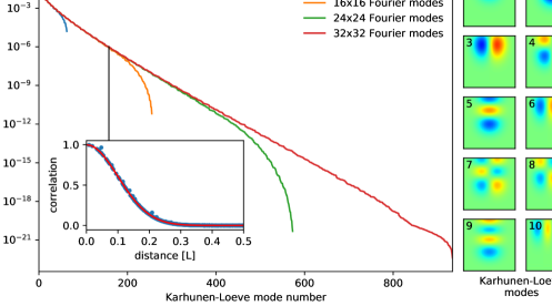
Figure 3: The eigenvalue spectrum $\Lambda$ of the $H_{K}$ matrix for a rupturing fault in three-dimensional space and a correlation length $\ell=0.1L$, computed at different truncation points of the trigonometric series. The inset shows the autocorrelation of the 153-mode Karhunen-Loeve expansion based on 1024 randomly selected point pairs (blue) along with the target autocorrelation function (red). Shown to the right are the first 10 Karhunen-Loeve modes $V\Lambda^{1/2}$.

For our experiments we set the correlation length to $\ell=5$ km and the slip amplitude to $\beta=1$ m. These values are representative of actual geophysical conditions but otherwise arbitrary. To determine the number of Karhunen-Loeve modes to retain, we set a maximum error of $\|H_{K}-V\Lambda V^{T}\|<$ 10 mm² measured in the Frobenius norm. By this process we establish that $n=12$ Karhunen-Loeve modes are sufficient for the 2D scenario and $n=153$ modes for the 3D scenario. Repeating this process for different truncation sizes of the original trigonometric series we find that this result is stable beyond 16 modes per dimension, and decide based on this that 32 basis functions per dimension is a sufficiently rich starting point for the expansion.

In a practical application one may wonder if the constructed prior distribution is an accurate representation of reality, and indeed if the true slip distribution is even an element of $\mathcal{B}$ at all. To make sure that a slip distribution drawn from the prior does not represent an artificial best case scenario with little real world value, we additionally construct a slip distribution that has local support at a select area of the fault. In addition to testing the robustness of the method to incorrect assumptions, the local support also allows us to test whether fault dimensions can indeed be captured via the slip, rather than via additional fault parameters.

4.3 Synthesizing observation data

We synthesize a displacement field for a given fault $m$ and slip distribution $b$ based on the assumption that that the free surface is flat and infinite, and the material properties are homogeneous. In this situation we have a fundamental solution available in the form of Melan’s (2D) and Mindlin’s (3D) solution, which means we can synthesize the displacement field by evaluating Volterra’s Equation (4). The integral is evaluated numerically by means of Clenshaw-Curtis quadrature up to a truncation error that is well below the selected noise level.

We fix Poisson’s ratio at $\nu=0.25$ for all experiments. The displacement field is evaluated in a uniformly spaced grid at a 50 meter resolution, covering the top of the search box defined in Section 4.1. The displacements are then projected onto a vector at a 30 degrees incidence angle, simulating line-of-sight observations as obtained from a typical satellite mission. Finally, Gaussian noise is added to the line-of-sight data that is spatially uncorrelated (thus ignoring atmospheric delays) and normally distributed with a standard deviation of 1 mm. A typical result can be seen in Figure 4. Note that, while the displacement is displayed without noise, the assumed noise is so small relative to the magnitude of the signal that adding it would not make a visible difference.

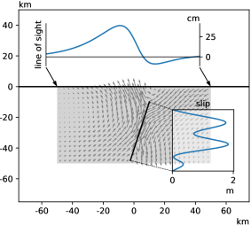
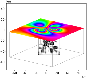
Figure 4: Visualisation of the search box containing a non-rupturing fault at position 10km ($0.2L$) and dip angle $72^{\circ}$ ($0.4\pi$), and in 3D additionally offset 5km ($0.1L$) and strike angle $54^{\circ}$ ($0.3\pi$) (Section 4.1), a slip distribution drawn from the prior distribution (Section 4.2) and corresponding synthesized deformation data at a $30^{\circ}$ incidence angle (Section 4.3). Left: a 2D scenario. Right: a 3D scenario in orthographic projection normal to the fault, showing line of sight deformations modulo 2.8 cm to mimic a typical C-band interferogram.

A difference between the raw synthesised data and deformation data received from a satellite mission is that the SAR sensor provides deformation data modulo the sensor’s semi-wave length (for details see e.g. [5]), measuring $d+k\lambda/2$ for an unknown integer value of $k$. While this is typically solved through phase unwrapping (under the assumption that $|\Delta d|<\lambda/4$ for adjacent points) it leaves the data inherently lacking an absolute reference. As we aim for this synthesized study to be representative of real world situations, we need to make sure that our measurement data is similarly relative. To this end we select one measurement point as a reference and subtract its deformation from that of the other measurement points. The inversion is then performed based on the differenced data, using a forward model that reflects the identical differencing procedure.

To formalize this procedure we introducing the unit vector $r\in\mathbb{R}^{n}$ that selects the reference point, and $e\in\mathbb{R}^{n}$ the vector of ones. With that we can express the differencing operator as

$$D=I-er^{T}.$$ (23)

The differencing is followed by a restriction operation that removes the reference point from the data, for which we introduce the operator $R\in\mathbb{R}^{n\times n-1}$. Note that $r$ and $R$ are related via $r^{T}R=0$ and $RR^{T}+rr^{T}=I$.

Regardless of the covariance of the measurement noise, all differenced data is correlated due to the shared reference point: $E((d_{i}-d_{\rm ref})(d_{j}-d_{\rm ref}))\neq 0$ in general due to the nonzero variance of $d_{\rm ref}$. Using the differencing and restriction operators we can express the covariance matrix of the differenced data in terms of that of the original measurements, which we shall denote henceforth as $\check{\Sigma}_{D}$:

$$\Sigma_{D}=R^{T}D\check{\Sigma}_{D}D^{T}R.$$ (24)

The additional covariances render the matrix fully dense. Fortunately, we note that we can express the inverse covariance of the differenced data in terms of that of the original measurements. Therefore, if the original covariance matrix can be inverted efficiently (for instance if it is diagonal) then this property carries over to the new covariance matrix:

$$\Sigma_{D}^{-1}=R^{T}X\check{\Sigma}_{D}^{-1}R,$$ (25)

where $X$ is a rank-1 update defined as

$$X=I-\frac{\check{\Sigma}_{D}^{-1}ee^{T}}{e^{T}\check{\Sigma}_{D}^{-1}e}.$$ (26)

While our choice of spatially uncorrelated noise implies that the covariance matrix is diagonal, (25) holds for any $\check{\Sigma}_{D}$ and is easily verified using the identities $D^{T}X=X$, $DX^{T}=D$ and $X\check{\Sigma}_{D}^{-1}=\check{\Sigma}_{D}^{-1}X^{T}$, together with $DR=R$, $RR^{T}D=D$ and $R^{T}R=I$. Using the same identities it further follows that

$$D^{T}R\Sigma_{D}^{-1}R^{T}D=X\check{\Sigma}_{D}^{-1}.$$ (27)

This last result (27) is noteworthy for two reasons. Firstly, in Equations (16) and (17) the inverse covariance occurs only surrounded by either the forward model or the data, both of which need to be differenced as $F_{m}=R^{T}D\check{F}_{m}$ and $d=R^{T}D\check{d}$. The result shows that it is not necessary to perform these operations explicitly, and that a rank-1 update of the original covariance matrix inverse is all it takes to switch from an inversion of absolute measurements to that of relative measurements. Secondly, the absence or $R$ and $r$ in (26) proves that the inversion is entirely insensitive to the chosen reference point — indeed, we do not need to make any choice at all.

4.4 Sampling the posterior distribution

We are interested in evaluating the expected value and auto-covariance of $M|D$, i.e. the posterior distribution of fault parameters given the measurements at the surface. The probability density function $f_{M|D}(m,d)$ was presented in (20). However, evaluation of this expression for a particular value of $m$ is problematic because of the marginal $f_{D}(d)$ contained within, which, while defined in Equation (8), does not have a closed form expression. As such we cannot feasibly evaluate the Lebesgue integral to compute the desired quantities.

We find a solution in the class of Markov Chain Monte Carlo (MCMC) methods, which provides an algorithm for drawing samples from $M|D$ while relying only on the ratio of the probability density function at two points $m_{1}$ and $m_{2}$, thereby cancelling the marginal and other factors that are independent of $m$. As the sample sequence $\{m_{1},m_{2},\dots\}$ thus produced has an empirical probability measure that coincides with the posterior distribution, the expected value and higher moments can be evaluated using Monte Carlo integration

$$E(g(M|D))=\lim_{N\rightarrow\infty}\frac{1}{N}\sum_{i=1\dots N}g(m_{i}),$$ (28)

for any $g$, which we can truncate at any $N$ depending on the desired level of accuracy.

While Equation (20) shows $f_{M|D}(m,d)$ to depend on $f_{M}(m)$, we stated in Section 4.1 that we take the prior distribution of $M$ to be uniform. As such the probability density function is proportional only to $\mathcal{N}_{\Sigma_{D}^{\prime}(m)}(d)$. Writing out the multivariate normal distribution and reworking terms we obtain the following identity:

$$\mathcal{N}_{\Sigma_{D}^{\prime}(m)}(d)=\frac{\exp(-\tfrac{1}{2}d^{T}\Sigma_{D}^{-1}d)}{\sqrt{(2\pi)^{\#\mathcal{D}}\det|\Sigma_{B}\Sigma_{D}|}}f_{d}(m),\quad f_{d}(m)=\frac{\exp(\tfrac{1}{2}d^{T}\Sigma_{D}^{-1}F_{m}b^{\prime}(m,d))}{\sqrt{\det|\Sigma_{B}^{\prime}(m)^{-1}|}}.$$ (29)

Here we made use of identity (19) to rewrite the determinant of the potentially very expensive covariance matrix $\Sigma_{D}^{\prime}(m)$ as the determinant of the smaller and less complex matrix $\Sigma_{B}^{\prime}(m)^{-1}$. We also isolated a proportionality constant independent of $m$, leaving only $f_{d}(m)$ to feature in our MCMC method.

Every evaluation of the resulting function involves a linear inversion of the slip for given $m$, as is seen directly from the presence of the posterior expected value $b^{\prime}(m,d)$ and covariance matrix $\Sigma_{B}^{-1}(m)$. The construction of these and of the forward model $F_{m}$ will be discussed in Section 4.5, which details the linear slip inversion process. Of note presently is that when the required inversion of $\Sigma_{B}^{-1}(m)$ is performed via a Cholesky decomposition, then the trace of the Cholesky matrix conveniently equals the square-root determinant in Equation (29).

The particular MCMC method selected for our purpose is the Metropolis-Hastings [6] algorithm, which performs a random walk through the sample space $\mathcal{M}$ using a proposal distribution to generate candidates, combined with an acceptance/rejection step based on the ratio of probability densities. The algorithm as it is employed here consists of the following steps:

1. initialize $m_{0}\in\mathcal{M}$

2. for $i=1,2,\dots,N$:

   1. draw a random update vector $\delta_{m}\in\mathcal{M}$ from the proposal distribution

   2. draw a uniform random number $u\in[0,1]$

   3. set $m_{i}=m_{i-1}+\begin{cases}\delta_{m}&\text{ if $f_{d}(m_{i-1}+\delta_{m})\geq uf_{d}(m_{i-1})$ (accept update)}\\ 0&\text{ otherwise (reject update)}\end{cases}$

Note that condition of step 2c implies that the update is always accepted if it leads to a state of higher probability. Note further that if an update is rejected the current state is repeated in the sequence, thereby adding weight to the empirical distribution and subsequent Monte Carlo integration (28).

What remains is to define the starting vector and the proposal distribution. While the proven convergence of the Markov chain suggests that both can be chosen arbitrarily if we take $N$ sufficiently large, this approach is not feasible in practice as the number of iterations required to escape from a local maximum can be prohibitively large. Instead, we require the starting point to be reasonably close to where $f_{d}$ takes its maximum, and the proposal distribution to be locally similar to $f_{d}$ in order to have a reasonable acceptance rate.

Aiming for the global maximum, we select the starting vector $m_{0}$ using a grid search to find local maxima followed by the Nelder-Mead uphill simplex method. The proposal distribution is taken to be Gaussian with covariance $\Sigma_{P}$, which we would like to resemble the distribution of $f_{d}$ local to $m_{0}$. Aiming to use a projection in logarithmic space, we wish to form a symmetric matrix $A$ such that, for all $\hat{m}$ in the vicinity of $m_{0}$,

$$-\tfrac{1}{2}(\hat{m}-m_{0})^{T}A(\hat{m}-m_{0})\approx\log f_{d}(\hat{m})-\log f_{d}(m_{0}).$$ (30)

As this relation is linear in the matrix coefficients $A_{ij}$ we can optimize it using the weighted linear least squares method, in which we reuse the sequence $\{\hat{m}_{i}\}$ of Nelder-Mead iterates as data points, and $f_{d}(\hat{m}_{i})$ as weights in order to downweigh the tails of the distribution. We note that, while it is convenient to reuse available data, we are at liberty to augment the series with extra evaluations in the vicinity of the optimum to increase the quality of the projection, even though we have found no need to do so for the cases considered.

Finally, we use the optimal scaling result of Roberts et al [15] to form the covariance matrix of our proposal distribution,

$$\Sigma_{P}=\frac{(2.38)^{2}}{\#\mathcal{M}}A^{-1}.$$ (31)

4.5 Evaluating the posterior expected slip

The expected value $E(B|MD)$ of the slip distribution given a fault $m$ and surface measurements $d$ is provided in closed form by Equation (17). The posterior covariance matrix is defined in Equation (16), in which $\Sigma_{B}$ is the identity matrix owing to the properties of the Karhunen-Loeve expansion. Crucially, both involve the formation of the forward model $F_{m}$, which maps the coefficient vector that encodes the slip distribution onto the corresponding vector of surface deformation gradients. It follows that the rows of the matrix $F_{m}$ are formed by the surface deformations corresponding to the slip distribution that is represented by the individual basis vectors $h_{n}(\xi)$ that we constructed in Section 4.2.

If the selected forward model is Volterra’s equation then $F_{m}$ is formed by repeated evaluation of Equation (4). If the selected model is the WSM then constructing $F_{m}$ involves constructing a finite element matrix and solving it for a block of right-hand-side vectors. Having discussed the evaluation of Volterra’s equation in Section 4.3, we will use the remainder of this section to elaborate on details of the latter.

A first step in any finite element computation is the formation of the computational mesh on which the discrete basis is formed, in our case to describe the displacement field. Recall from Section 4.1 that all fault planes $\mathcal{M}$ will be confined in a rectangular box of given size. We now create a regularly spaced grid of elements spanning this search box, allowing us to cheaply trace any physical coordinate inside the box to the containing element and its element-local coordinate which will greatly aid the efficiency of the fault plane integration. We note, however, that efficient lookup procedures exist for other mesh types as well, for example using quad trees [8] or alternating digital trees [2].

Since our computational domain is a halfspace we have no boundary conditions to place on the walls of the search box, except for the free surface which is traction free. Instead we take the infinite element approach of extending our mesh with several rows of extra elements and using a geometric map to continuously stretch the elements outside the search box towards infinity. Specifically, if $2L$ is the width of the box, $2n_{\rm box}$ the number of elements spanning the box and $2n_{\rm inf}$ the number of elements spanning infinity, we apply the following piecewise hyperbolic map to every spatial dimension:

$$x_{i}(e)=\frac{L}{n_{\rm box}}\left\{\begin{array}[]{ll@{\ }l}e-(n_{\rm box}+e)^{2}/(n_{\rm inf}+e)&-n_{\rm inf}&<e<-n_{\rm box}\\ e&-n_{\rm box}&\leq e\leq+n_{\rm box}\\ e+(n_{\rm box}-e)^{2}/(n_{\rm inf}-e)&+n_{\rm box}&<e<+n_{\rm inf}\end{array}\right.$$ (32)

Note that this includes the depth direction, in which case we take $-n_{\rm inf}<e\leq 0$. Unless stated otherwise we will select a infinity-to-box ratio of $n_{\rm inf}/n_{\rm box}=\tfrac{3}{2}$, which means that in 3D the treatment of the far field increases the number of elements by a factor $(\tfrac{3}{2})^{3}\approx 3.38$ relative to the number of elements in the search box.

In creating the discrete function space $V_{n}$ we make use of the fact that our mesh is structured by creating a C¹ quadratic spline basis, also known as isogeometric analysis [7], which we showed in [20] to have better accuracy to degrees of freedom, and we remove the outermost basis functions to impose the far field constraint. With that we are in a position to evaluate the left hand side of Equation (6) to form the stiffness matrix. Since this matrix will be reused many times we also invest the time to construct a high quality preconditioner, opting, in fact, to form a complete Cholesky decomposition.

The right-hand side of Equation (6) involves an integral over $\mathcal{X}$ for which we use the same Clenshaw-Curtis quadrature scheme that we used for the synthetization of observation data in Section 4.3, while making use of the rectilinearity of the mesh in the search box to locate the corresponding element coordinates necessary to evaluate the basis functions. Having formed the right-hand side vector we can solve the system and form the discrete solution $u_{h}\in V_{n}$, which can then be evaluated in any point of our choosing.

5 Results

We will present several results of the process outlined in Section 4, with the aim of illustrating the many variables and their effect on the overall computation. While we are mainly interested in applications in three-dimensional space, we find that most computational aspects appear identically in the two-dimensional analogue. Appreciating the advantages for visualisation we therefore present most of our observations in this setting, adding 3D results mainly to confirm these findings. For structure we will use the scenarios of Figure 4 as a baseline test case, with minor modifications where required.

5.1 Linear inversion: slip distribution

We will study first the linear inversion process, in which we keep the fault parameters $m$ equal to the exact values and invert the slip distribution $b$ only — referring to the methodology of Section 4 we set $\tilde{m}=m$ in step 4. A natural starting point is to establish the best case solution by inverting using Volterra’s equation, the forward model that was used to synthesize the data. The results of this are shown in Figure 6. While the inverted slip distribution does not match the exact slip due to the smoothing effect of the prior distribution, we observe in the left panel a reasonable fit that is in keeping with the posterior variance. In the right panel we observe that the deformation error stays well below the 1 mm measurement noise standard deviation.

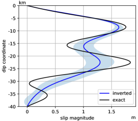
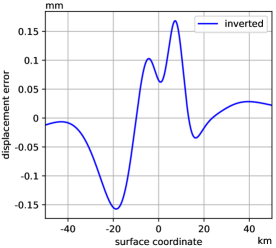
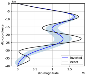
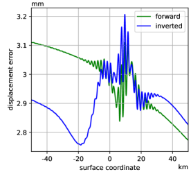
Figure 5: Linear inversion of the slip distribution in the 2D non-rupturing scenario of Figure 4 using Volterra’s equation. Left: The exact slip distribution $b$, the inverted slip distribution $b^{\prime}(m,d)$, and the one standard deviation, 68% confidence interval $\pm\sqrt{h^{T}\Sigma_{B}^{\prime}(m)h}$. Right: The difference between the exact surface deformation and the deformation that corresponds to the inverted slip distribution $b^{\prime}(m,d)$ using Volterra’s equation as the forward model.

Figure 6: Linear inversion of the slip distribution in the 2D non-rupturing scenario of Figure 4 using the WSM forward model on a $76\times 38$ element mesh, of which $50\times 25$ elements form the search box. The graph layout is identical to that of Figure 6, with the addition of the ‘forward’ deformation error that corresponds to the exact slip distribution, rather than the inverted slip distribution.

Repeating this process with the WSM on a $76\times 38$ element mesh we obtain the result of Figure 6, showing that the expected slip and standard deviation are almost identical to those obtained using Volterra’s equation. Paradoxically, the corresponding deformation error in the right panel (‘inverted’) is relatively large. It is noteworthy that the deformation error is characterized by a significant offset (approximately 3 mm) with a relatively small variation (approximately 0.2 mm). A similar offset can be seen in the (‘forward’) error that the model produces with the exact slip as input, thus representing the discretization error for this particular computational setting. From this we can conclude that the offset does not result from the inversion process, but is in fact a side effect of the discrete model. Fortunately, by virtue of the differencing approach layed out in Section 4.3, the inversion is insensitive to offsets of this kind. We observe that the errors are small relative to the offset, with a peak to peak error range that is well below 1 mm, which explains the perceived paradox.

In addition to the 3 mm offset, the forward error curve of Figure 6 shows a distinct spatial trend, dropping by 0.35 mm over the length of the domain. Both aspects of the discretization error are studied in Figure 8, which shows two variations of the mesh resolution. On the left we see the effect of increasing the resolution in the far field while keeping that in the search box fixed. Comparing to Figure 6, we observe that both the offset and the trend are greatly reduced, indicating that these phenomena are caused largely by the treatment of the far field. At the same time the errors did not change significantly relative to the offset, confirming that this far field-induced error should not strongly affect the inversion. On the right we see how an eight-fold uniform mesh refinement results in a stark reduction of the discretization error, and in an inverted deformation error that closely resembles that of the baseline result of Figure 6 modulo the remaining offset and trend.

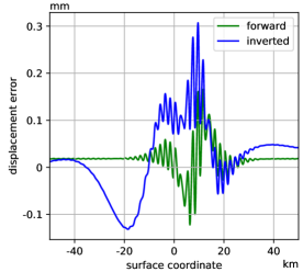
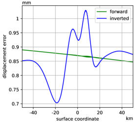
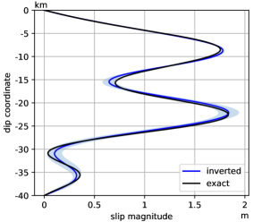
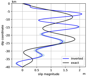
Figure 7: Linear inversion of the slip distribution in the identical setting to Figure 6 except for different finite element meshes. Referencing Equation (32), the baseline mesh was constructed for $n_{\rm box}=25$ and $n_{\rm inf}=38$, resulting in a $76\times 38$ element mesh of which $50\times 25$ elements form the search box. Left: $n_{\rm box}=25$ and $n_{\rm inf}=200$, keeping the search box resolution fixed while adding elements to the far field. Right: $n_{\rm box}=100$ and $n_{\rm inf}=150$, keeping the infinity-to-box ratio fixed while increasing resolution by a factor 4.

Figure 8: Linear inversion of the slip distribution in the identical setting to Figure 6 except for a 100$\times$ reduction of the measurement noise to 0.01 mm. Left: Volterra-based inversion. Right: WSM-based inversion on a $76\times 38$ element mesh, of which $50\times 25$ elements form the search box. This is an illustration of the adverse effects on the inversion when the noise level undercuts the discretization error.

Taken together, the results of Figure 8 uphold the result of [20] that the discretization error can be made arbitrarily small via mesh refinement. However, as we have already seen, it is by no means necessary to drive the error orders below the noise level of the deformation measurements. To see what happens in the opposite direction, Figure 8 compares the Volterra and WSM-based inversion at a noise level that is 100 times smaller while maintaining the mesh. While Volterra’s equation correctly tightens the error margin around the exact slip, the WSM-based inversion deviates significantly from the exact slip due to the dominant numerical error. At this noise level it takes an eightfold uniform mesh refinement for the WSM-based inversion to return to being indistinguishible from the Volterra based inversion, beyond which the inversion is essentially mesh-independent. Based on these results, we consider that a mesh at which the discretization error does not exceed half the standard deviation of the measurement noise appears to strike a good balance between accuracy and numerical efficiency.

There is one situation where we cannot control the discretization error through mesh refinement, which is in the case of a rupturing fault. As the approximation is inherently continuous, the error at the point of intersection equals half the slip magnitude regardless of element size. Since this violates the established rule that the discretization error may not exceed the measurement noise, care must be taken to avoid the detrimental effects we observed in the right panel of Figure 8. Arguably the simplest way to achieve this is to discard measurements close to the rupture and use only the remaining intermediate to far field data. Incidentally, the masking out of data in the rupture zone is not uncommon in the context of SAR interferometry, as local destruction tends to lead to decorrelation of the radar signal. We hypothesize, therefore, that no valuable data need be discarded in practice.

An example of a rupturing fault can be seen in Figure 10. The right panel shows the absolute displacement (rather than the displacement error) in which we observe continuous oscillations at the 10 km position where the exact displacement exhibits a discontinuity. The oscillations decay rapidly, reaching sub-millimeter scale amplitudes at a 10 km distance from the surface rupture. The left panel shows the inversion result based on the deformation data outside of this $\pm 10$ km interval that is marked gray in the right panel. The result accurately recovers the exact slip distribution, and is virtually indistinguishable from the Volterra-based inversion (not displayed) subject to the same data mask, confirming that data masking is a suitable strategy to deal with the continuous representation of discontinuities in the WSM.

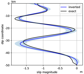
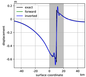
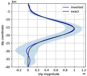
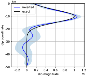
Figure 9: Linear inversion of the slip distribution in a 2D rupturing scenario. The graph layout is similar to that of Figure 6, with the difference that the right panel shows the absolute displacements rather than the displacement errors with the black ‘exact’ curve representing the synthesized displacement field. The gray band in the the right panel corresponds to the area that was masked out in order for the locally meter-scale errors not to affect the inversion.

Figure 10: Linear inversion of a manually constructed Gaussian slip distribution in a 2D scenario, solved on a $76\times 38$ element mesh. Left: a non-rupturing scenario with the slip centered at 40% dip. Right: a rupturing scenario with the slip centered at 20% dip and a masked area of 20 km.

So far we have drawn a slip distribution from the prior distribution, the same that is subsequently used in the inversion procedure to reconstruct the slip from measurements. Since it is difficult in practice to accurately capture prior knowledge in terms of a distribution, it is relevant to study the robustness of the procedure to slip distributions not being elements of our discrete space $\mathcal{B}$. Examples of this can be seen in Figure 10, which shows two Gaussian slip distributions, one rupturing, the other non-rupturing. Though neither is a member of $\mathcal{B}$, both distributions are recovered with reasonable accuracy, confirming that the methodology has at least some lenience to inadequacies in the choice of the prior. This also confirms our premise that the size of the fault plane need not be an independent parameter if we have reasonable upper bounds, as the areas of zero slip are captured accurately.

Finally we turn to the 3D scenario (right panel) of Figure 4. Employing the identical methodology, Figure 11 shows the slip distribution and the corresponding error in deformation gradient, in which we recognize similar patterns to those we observed in the direct 2D equivalent of Figure 6. Taking into account the local standard deviation, the inverted and exact slip distributions are in good agreement. We also confirmed that the result is indistinguishable from that obtained via Volterra’s equation. The error is largest in the vicinity of the fault, but stays well clear of the 1 mm noise level. Interestingly, the error offset that we observed in the 2D results is much less pronounced in the 3D situation.

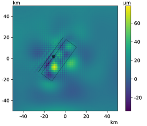
Figure 11: Linear inversion of the slip distribution in a 3D non-rupturing scenario using the WSM forward model on a $76\times 76\times 38$ element mesh, of which $50\times 50\times 25$ elements form the search box. Left: The exact slip distribution $b$ as black quivers, the inverted slip distribution $b^{\prime}(m,d)$ as blue quivers, and the local one standard deviation or 47% confidence region resulting from the $2\times 2$ posterior covariance matrix $h^{T}\Sigma_{B}^{\prime}(m)h$ as blue ellipses, centered at the expected value and at matching scale. Right: the vector norm of the deformation gradient error. The solid rectangle shows the outline of the fault plane.

5.2 Nonlinear inversion: fault parameters

We proceed by studying the nonlinear inversion of the fault parameters. Referring again to the methodology of Section 4, in step 4 we now evaluate the posterior expected value for the fault parameters $m$ using the Metropolis-Hastings MCMC process. This process samples the posterior distribution through repeated evaluation of $f_{d}(m)$ as defined in Equation (29), being proportional to the posterior probability density function $f_{M|D}$. As this entails evaluation of the expected value $b^{\prime}(m,d)$, all aspects of the linear inversion process as explored in the previous section remain in effect.

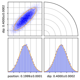
             position [$L$]              dip angle [$\pi$]                             position [$L$]              dip angle [$\pi$]

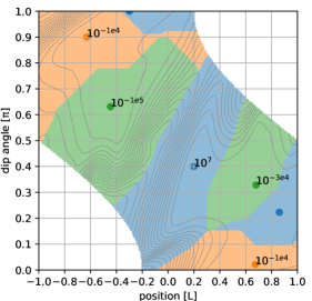
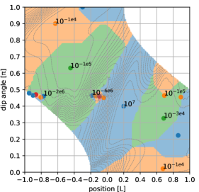
Figure 12: Binned results of a 50.000-sample MCMC process for $M|D$ using Volterra’s equation in the 2D non-rupturing scenario of Figure 4, which has fault parameters position=$0.2L$ and dip angle=$0.4\pi$. Left: reference results from Volterra’s equation. Right: results from the WSM on a $48\times 24$ element mesh, of which $32\times 16$ elements form the search box. The bottom row shows the marginalized distributions for fault position (left) and the dip angle (right), with axis labels showing mean value $\pm$ standard deviation or, equivalently, the 68% confidence interval. The orange overlay shows the corresponding normal distribution. Grid lines are spaced at one standard deviation. The top row shows the cross correlation of x coordinate and dip angle, with the orange overlay showing the bivariate normal distribution at two standard deviations or, equivalently, the 91% confidence region.

Figure 13: Contour lines and local maxima of $f_{M|D}$ for the same 2D non-rupturing scenario as that of Figure 13. The coloured areas represent (inverse) watersheds of the probability landscape, that is, the collection of points from which an uphill gradient method converges to the associated local maximum. Left: reference result from Volterra’s equation. Right: results from the WSM on a $48\times 24$ element mesh.

Returning to the non-rupturing 2D baseline scenario (left panel) of Figure 4, Figure 13 shows the results of a MCMC process comparing Volterra’s equation to the WSM. We use the same relatively coarse mesh that we used for Figure 6 to see if there are adverse effects in pushing against the boundary of the discretization error. Both distributions are seen to capture the fault parameters correctly, pinpointing the exact values to a high degree of accuracy both in terms of a nearly exact expected value and of the equally narrow confidence interval. Furthermore, both distributions are in excellent agreement to each other, demonstrating the robustness of the method with regard to discretization errors.

We started the MCMC random walk from the global maximum, obtained via the Nelder-Mead uphill simplex method, that in turn was started from where we know the exact solution to be. Knowledge of an exact solution is a luxury that is not available in any practical application, which means a global search algorithm will typically be required to prepare for the final gradient ascent. A relevant question, therefore, is whether the WSM has a disturbing effect in this regard. To explore this, Figure 13 compares the posterior probability density function obtained through direct evaluation of Volterra’s equation against that obtained via the WSM, identifying local maxima as well as the associated watersheds. While the WSM introduces some spurious local maxima, the global maximum as well as its watershed appear identical, suggesting that there is no difference with regard to global optimization strategies.

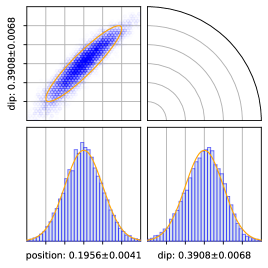
             position [$L$]              dip angle [$\pi$]                             position [$L$]              dip angle [$\pi$]

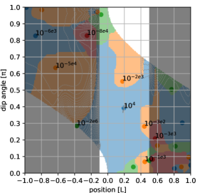
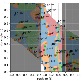
Figure 14: Binned results of a 50.000-sample MCMC process for $M|D$ using the WSM forward model in a 2D rupturing scenario with the same parameters as in Figure 13: position=$0.2L$ and dip angle=$0.4\pi$. A radius $0.3L$ data mask is applied centered at x=$0.2L$. Left: reference results from Volterra’s equation. Right: results from the WSM on a $96\times 48$ element mesh, of which $64\times 32$ elements form the search box.

Figure 15: Contour lines, local maxima and watersheds of $f_{M|D}$ for the same 2D non-rupturing scenario as that of Figure 15, with an overlay delineating the masked region. Left: reference result from Volterra’s equation. Right: results from the WSM on a $96\times 48$ element mesh.

For the rupturing scenario we mask out an area of 30 km centered at the point of rupture. While it may seem contradictory to mask out the rupture zone while simultaneously inverting for the rupture coordinate, this process should be understood in the context of having prior information in the form of in situ observations. Even though the precise trajectory of the rupture may not be known to sufficient accuracy, it may well be sufficient to define a masking zone. In fact, though not employed here, we are at liberty to modify the prior distribution to have it reflect this knowledge as well. Selecting the uniformly refined grid of Figure 10, the 30 km zone is 50% wider than the observed minimum in order to not artificially limit mobility of the rupture coordinate, but rather give it some freedom to find its optimum within the confines of the broader mask.

Figure 15 shows the side by side results of Volterra’s equation and the WSM. Note that the mask was applied to Volterra’s equation as well for sake of comparison, even though the method does not require it. The distributions in the rupturing scenario are less precise as a result of data masking, but are otherwise in excellent agreement.

Figure 15 again explores the posterior probability density function, where this time we see a very large qualitative difference between Volterra’s equation and the WSM. While both show a clear delineation at $(0.2\pm 0.3)L$, corresponding to the applied data mask, the WSM produces many more local maxima, clustering in particular at the crossover points and at shallow dip angles. The global maximum still has a fairly large associated watershed, however, suggesting that the multitude of local maxima is not necessarily problematic in a global optimization context. Note also that the global optimization algorithm needs only consider positions inside the masked region — the non-shaded region in the figure — as ruptures outside of the mask are in violation of its premise.

We conclude again with the 3D scenario (right panel) of Figure 4. Using the same mesh as was used for the slip inversion of Figure 11, Figure 16 shows the posterior distribution of the 3D fault parameters. One can observe that the expected values accurately match the parameters that were used to generate the synthetic data. The position along strike has a markedly larger variance than that perpendicular to it, which matches the expectations laid out in Section 4.1 relating to ambiguities with the slip distribution. Though we cannot feasibly run the MCMC process using Volterra’s equation to verify the correctness of this result, we consider the foregoing to be sufficient support to present this as a demonstration of the WSM driving a realistic, nonlinear inversion of a 3D fault plane.

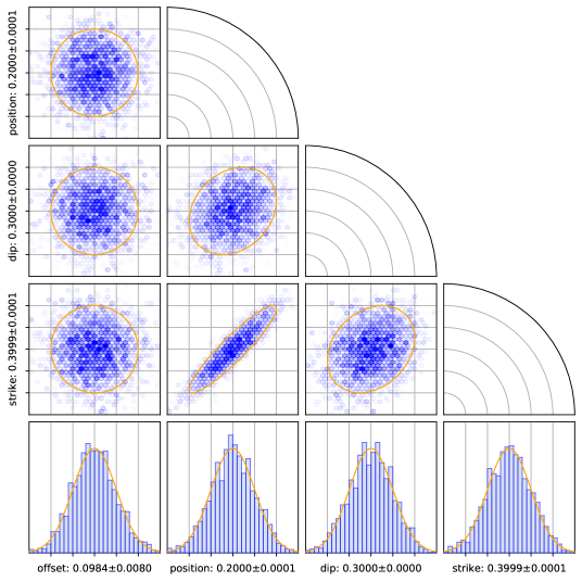
                offset [$L$]                 position [$L$]              strike angle [$\pi$]            dip angle [$\pi$]

Figure 16: Binned results of a 10.000-sample MCMC process for $M|D$ corresponding to the 3D non-rupturing scenario of Figure 4, which has fault parameters offset=$0.1L$, position=$0.2L$, strike angle=$0.3\pi$ and dip angle=$0.4\pi$. The bottom row shows from left to right the marginalized distributions for fault offset, position, strike and dip, with axis labels showing mean value $\pm$ standard deviation or, equivalently, the 68% confidence interval. The orange overlay shows the corresponding normal distribution. Grid lines are spaced at one standard deviation. The remaining rows show from top to bottom the fault parameters y, strike and dip, thus covering all cross correlations. The orange overlay shows the bivariate normal distribution at two standard deviations or, equivalently, the 91% confidence region.

6 Conclusions

In this paper we performed for the first time a full inversion of fault plane parameters and fault slip distribution using the Weakly-enforced Slip Method (WSM) that was developed explicitly for this purpose. By restricting the domain to a homogeneous halfspace we were able to synthesize deformation data, as well as compare the WSM-based inversion against a reference result obtained from the exact solution. This allowed us to study in detail the effect that the discretization error has on different aspects of the inversion process. To provide our study with a mathematical framework we placed the inverse problem in a Bayesian setting, in which a prior probability distribution is refined though observations into a posterior probability that quantities the likelihood of various faulting mechanisms.

For linear inversions, the WSM was found to be competitive with Volterra’s equation in terms of accuracy, showing excellent agreement already at coarse meshes (5 elements per 10 km for the situation considered) in case of non-rupturing faults. As a practical rule of thumb for the minimum required mesh density, we demonstrated empirically that the discretization errors must not exceed the standard deviation of the measurement noise in order to avoid large numerical errors. Conversely, increasing the mesh density beyond this point contributes little to the accuracy of the inversion.

A WSM-based inversion of rupturing faults requires additional measures to account for the local smearing out of the discontinuity, but it is argued that similar measures are often required in practice regardless. When a simple data mask is applied to disregard data points in the vicinity of the rupture, the WSM and exact method again show excellent agreement, albeit at a finer mesh that is required to localize the discrization error to the rupture zone. Local to the rupture the error is observed to decay exponentially, at a rate that is inversely proportional to the element size of the computational mesh. It is expected that this relation holds as well in the case of local, rather than uniform, refinements.

While the WSM was originally analyzed on a finite domain with exact boundary conditions [19], real world applications cannot rely on the availability of such data. Instead of introducing artificial boundaries, we opted for a finite-to-infinite mapping for the treatment of the far field in order not to introduce assumptions that might limit the validity of our results. Though this treatment introduces a fairly significant error, we observe that the relative displacement error of two nearby points remains dictated by the local element size. This circumstance fits remarkably well with the fact that satellite-based InSAR observations are inherently relative, which means that treatment of the data must be insensitive to global offsets. While successful in this regard, meshing the far field is arguably an expensive solution, increasing the number of degrees of freedom by a factor 3.38 in the test cases considered. Further study in this direction is therefore warranted.

For non-linear inversions, any global search algorithm followed by a gradient-based optimization is shown to perform equally well for the WSM as it does for the exact forward method, as demonstrated by a full comparison of the posterior probability density. Furthermore, we demonstrated that the iterates of the Nelder-Mead uphill simplex method can be reused in a linear least squares projection to provide a high quality Gaussian proposal distribution for a subsequent exploration of the posterior probability using the Metropolis-Hastings Markov Chain Monte Carlo method.

In an observation that is unrelated to the WSM we have remarked that certain parameters that are customarily added to the space of fault parameters, such as the fault plane dimensions, can instead be captured at lesser cost by the slip distribution. In situations where an ambiguous relationship remains between a fault parameter and the slip distribution, this translates to a large variance of the posterior distribution, as demonstrated by the along-strike offset of the fault plane in the 3D scenario.

In conclusion, we believe that the present work convincingly demonstrates the utility of the WSM in real world applications, combining the power and flexibility of finite element analysis with a highly efficient reuse of computational effort. It also provides a practical framework by which such studies can be performed. While the current experiments have been restricted to homogeneous halfspaces for reasons of verification, none of these restrictions were required by the methodology as it is presented here; nor do we have reason to believe that our findings are limited to these conditions.

References

- [1] J. Biggs and T.J. Wright. How satellite insar has grown from opportunistic science to routine monitoring over the last decade. Nature Communications, 11(3863), 2020.
- [2] J. Bonet and J. Peraire. An alternating digital tree (adt) algorithm for 3d geometric searching and intersection problems. Numerical Methods in Engineering, 31, 1991.
- [3] J. Elliott, R. Walters, and T. Wright. The role of space-based observation in understanding and responding to active tectonics and earthquakes. Nature Communications, 7(13844), 2016.
- [4] Y. Fialko, D. Sandwell, M. Simons, and et al. Three-dimensional deformation caused by the bam, iran, earthquake and the origin of shallow slip deficit. Nature, 435:295–299, 2005.
- [5] R.F. Hanssen. Radar Interferometry. Springer Netherlands, 2001.
- [6] W.K. Hastings. Monte carlo sampling methods using markov chains and their applications. Biometrika, 57:97–109, 1970.
- [7] T. Hughes and J.A. Evans. Isogeometric analysis. Technical Report 10-18, ICES, 2010.
- [8] R. Krause and E. Rank. A fast algorithm for point-location in a finite element mesh. Computing, 57:49–62, 1996.
- [9] A.E.H. Love. A treatise on the mathematical theory of elasticity. Dover publications, 4th edition, 1927.
- [10] M. Loève. Probability Theory I, chapter Elementary probability theory, pages 1–52. Springer, 1977.
- [11] E. Melan. Der spannungszustand der durch eine einzelkraft im innern beanspruchten halbscheibe. Zeitschrift für Angewandte Mathematik und Mechanik, 12(6):343–346, 1932.
- [12] R.D. Mindlin. Force at a point in the interior of a semi‐infinite solid. Journal of Applied Physics, 7(5):195–202, 1936.
- [13] Y. Okada. Internal deformation due to shear and tensile faults in a half-space. Bulletin of the Seismological Society of America, 82(2):1018–1040, 1992.
- [14] W. Prescott. Seeing earthquakes from afar. Nature, 364:100–101, 1993.
- [15] G.O. Roberts, A. Gelman, and W.R. Gilks. Weak convergence and optimal scaling of random walk metropolis algorithms. The Annals of Applied Probability, 7(1):110–120, 1997.
- [16] P. Segall. Earthquake and Volcano Deformation. Princeton University Press, 2010.
- [17] M. Simons, Y. Fialko, and L. Rivera. Coseismic deformation from the 1999 mw 7.1 hector mine, california, earthquake as inferred from insar and gps observations. Bulletin of the Seismological Society of America, 92(4):1390–1402, 2002.
- [18] A. Tarantola. Inverse Problem Theory and Methods for Model Parameter Estimation. SIAM, 2005.
- [19] G.J. van Zwieten, R.F. Hanssen, and M.A. Gutiérrez. Overview of a range of solution methods for elastic dislocation problems in geophysics. Journal for Geophysical Research: Solid Earth, 118(4):1721–1732, 2013.
- [20] G.J. van Zwieten, E.H. van Brummelen, K.G. van der Zee, M.A. Gutiérrez, and R.F. Hanssen. Discontinuities without discontinuity: The weakly-enforced slip method. Computer Methods in Applied Mechanics and Engineering, 271:144–166, 2014.
- [21] V. Volterra. Sur l’équilibre des corps élastiques multiplement connexes. Annales scientifiques de l’École Normale Supérieure, 24:401–517, 1907.
- [22] W. Xu, R. Dutta, and S. Jónsson. Identifying active faults by improving earthquake locations with insar data and bayesian estimation: The 2004 tabuk (saudi arabia) earthquake sequence. Bulletin of the Seismological Society of America, 105(2A):765–775, 2015.
- [23] E.H. Yoffe. The angular dislocation. The Philosophical Magazine: A Journal of Theoretical Experimental and Applied Physics, 5(50):161–175, 1960.
- [24] O.C. Zienkiewicz, R.L. Taylor, and J.Z. Zhu. The Finite Element Method: Its Basis and Fundamentals. Butterworth-Heinemann, 2013.