Abstract
Diffuse low grade gliomas are slowly growing tumors that always recur after treatment. In this paper, we revisit the modeling of the tumor radius evolution before and after the radiotherapy process and propose a novel model that is simple, yet biologically motivated, and that remedies some shortcomings of previously proposed ones. We confront it with clinical data consisting in time-series of tumor radius for 43 patient records, using a stochastic optimization technique and obtain very good fits in all the cases. Since our model describes the evolution of the tumor from the very first glioma cell, it gives access to the possible age of the tumor. Using the technique of profile-likelihood to extract all the information from the data, we build confidence intervals for the tumor birth age and confirm the fact that low-grade glioma seem to appear in the late teenage years. Moreover, an approximate analytical expression of the temporal evolution of the tumor radius allows us to explain the correlations observed in the data.
keywords:
Mathematical modeling; gliomas; radiotherapy; optimization; data analysis1 \issuenum1 \articlenumber0 \datereceived \dateaccepted \datepublished \hreflinkhttps://doi.org/ \TitleRadiotherapy Effects on Diffuse Low-Grade Gliomas: Confronting Theory With Clinical Data \TitleCitationRadiotherapy effects for diffuse low-grade gliomas \AuthorLéo Adenis1,2, Stéphane Plaszczynski1,2*, Basile Grammaticos1,2, Johan Pallud 3,4,5 and Mathilde Badoual1,2 \AuthorNamesLeo Adenis, Stephane Plaszczynski, Basile Grammaticos, Johan Pallud and Mathilde Badoual \AuthorCitationAdenis, A.; Plaszczynski, S.; Grammaticos, B.; Pallud ,J; Badoual, M. \corresCorrespondence: stephane.plaszczynski@ijclab.in2p3.fr
1 Introduction
Gliomas are tumors of the central nervous system that arise from precursors of glial cells and account for almost 80% of primary malignant brain tumors. Although relatively rare, they result in more years of life lost than any other tumor: approximately 13000 deaths and 18000 new cases of primary malignant brain and central nervous system tumors occur annually in the US Louis et al. (2007). Historically, the tumors of the central nervous system have been classified by the World health organization into four grades, based on their histological characteristics and reflecting the aggressiveness of the tumor Louis et al. (2007): grade 1 gliomas are benign, well delineated and can be cured by surgery. From grade 2 and above, the tumors are diffuse and because of that, incurable. Recently, a revision of the World Health Organization classification was proposed, reflecting the fact that prognosis is more strongly associated with molecular diagnostic features than with histological ones only Louis et al. (2016). It is now the isocitrate dehydrogenase (IDH) enzyme mutation status that allows to classify these tumors in the first place. According to this revision, the group of grade 2 low-grade gliomas now includes diffuse astrocytomas (mutant IDH1) and oligodendrogliomas (mutant IDH1 and 1p/19q co-deletion). The highest grade glioma group, that includes IDH wildtype glioblastomas and grade 3 astrocytomas, is associated with a life time expectancy of less than a year Marra et al. (2019). In this paper, we use data from patients who were recruited before 2016 for most of them. The status of the IDH enzyme mutation was not assessed and the gliomas were classified according to histological features only. We have just followed the WHO classification in use at the time of diagnosis and use the term of diffuse low-grade gliomas (DLGG) for these patients’ tumors, that includes low-grade astocytomas and oligodendrogliomas Pallud et al. (2012).
In high-grade gliomas, the rate of proliferation is very large and in the center, the cells become hypoxic and finally necrotic. In contrast, in DLGG, the rate of proliferation is lower, and these tumors are composed only of isolated migrating tumor cells that infiltrate the normal tissue. On a MRI scan, DLGG present a T1 hypointense signal without contrast enhancement (since there is no angiogenesis) but a T2-FLAIR hyperintense signal Pallud and Mandonnet (2011); Price (2010). It has been shown that tumor cells migrate well beyond the tumor limits of this hyperintense area on T2-FLAIR weighted MRI scans Kelly et al. (1987); Pallud et al. (2010a).
If DLGG are associated to an extended lifetime expectancy compared to higher-grade gliomas, they represent a real public health issue since patients are often young (between 20 and 40 years-old) with a previously normal social and professional life. DLGG grow slowly but their invasive feature is responsible for the unavoidable recurrence, even after oncological treatments Pallud et al. (2010b).
Treatments consist in the first place in surgery when possible. Chemotherapy and then radiotherapy are proposed in front of a progressive residual tumor and at tumor progression. However, despite technical progress in imaging techniques and therapeutic management, treatment only confers a modest improvement in overall survival Ricard et al. (2007); Peyre et al. (2010); Mandonnet et al. (2009); Prabhu et al. (2010). But even worse, all low-grade lesions eventually evolve into higher-grade malignant tumor, when neoangiogenesis is triggered Bobek-Billewicz et al. (2014).
For DLGG, the goals of radiotherapy (RT) are to control tumor growth, improve progression-free survival and patient quality of life by reducing the risk of seizures, and delay anaplastic transformation van den Bent et al. (2005).
Several aspects of DLGG have already been the object of models, from their origin Dufour et al. (2018) to their natural evolution Mandonnet et al. (2009); Gerin et al. (2012), their response to treatments (in particular with RT Ribba et al. (2012); Badoual et al. (2014); Perez-García et al. (2015); Galochkina et al. (2015); Budia et al. (2019)) and their anaplastic transformation Bogdanska et al. (2017). The diffusion-proliferation model plays a special role in the modeling of glioma evolution field. It is based on a differential equation governing glioma cell density, and in its simplest form, involves only two key phenomena (and thus two parameters): the migration (modeled as a diffusion) of the cells and their proliferation. This model has been extensively used for high-grade gliomas Harpold et al. (2007); Badoual et al. (2010); Corwin et al. (2013); Unkelbach et al. (2014); Amelot et al. (2017), but in fact, the model is more adapted to DLGG. Despite its simplicity, this model can reproduce in particular an important feature of DLGG growth that has been verified with clinical data, which is that the tumor radius increases linearly with time (at large time) Mandonnet et al. (2003); Pallud et al. (2006).
The most striking feature of the evolution of DLGG under RT, that any model should reproduce, is that the tumor radius continues to decrease even after the end of the treatment. This delay can range form a few months to almost ten years, depending on the patient, before the tumor systematically recurs, and starts to grow again. In Ribba et al. (2012) two populations of cells are defined, one that is quiescent and the other one that proliferates. RT damages the cells of the proliferating population, thus transforming them into quiescent cells. The model is based on ordinary differential equations and does not include any spatial structure. However, in the case of gliomas, the spatial structure is essential in a model since a key feature of DLGG is their capacity to invade surrounding normal tissue. In Rockne et al. (2010) the authors use the diffusion-proliferation model, with cell death term due to RT (present only while the therapy lasts), and apply it to high-grade gliomas. But this model is not adequate for low-grade gliomas since it cannot account for the most striking feature of the clinical follow up, i.e. the reduction of tumour radius that lasts much longer than the treatment by RT itself. In Badoual et al. (2014) our group proposed a diffusion-proliferation model coupled with the production of edema by tumor cells. We fitted successfully 29 follow-ups of patients. However, even if this model is the closest to the biological characteristics of DLGG, it involves 5 parameters, including the two parameters for the edema dynamics. These two parameters are unknown and cannot be easily measured experimentally. Without any estimation of their values to compare with, it is difficult to validate the model and make predictions. In Perez-García et al. (2015), the authors developed a model based on the diffusion-proliferation model that involves two cell populations, the damaged by RT and the not damaged one, close to the one in Ribba et al. (2012). The advantage of this model is that it contains a spatial structure and also allows a slow decrease of the tumor radius after the end of the RT treatment. The authors used the model to study the impact of a fractionation of the RT treatment Galochkina et al. (2015); Henares-Molina et al. (2017). However, these studies are theoretical and the model was not applied to real clinical data.
In this article, we develop a simple biophysical model of DLGG evolution based on the diffusion-proliferation model with the addition of the effect of RT and confront it to a large number (43) of patients clinical data. We use state-of-the art analysis techniques to adjust the model and show that it is possible to get an excellent agreement between the model and the data, for all the patients. We then study the birth age of the tumors, the parameter values and the correlations among several observables before and after RT.
2 Materials and Methods
2.1 The patients
We had at our disposal a set of 43 patients with DLGG, diagnosed at the Sainte-Anne Hospital (Paris, France) from 1989 to 2000. These patients were selected according to precise criteria detailed elsewhere Pallud et al. (2012). In short, only adults with typical DLGG (that is, no angiogenesis and thus no contrast enhancement on gadolinium- T1 images), available clinical and imaging follow-up before, during, and after RT and RT as their first oncological treatment except for stereotactic biopsies, were eligible. The patients had MRI follow-up before, during and after RT. Three tumour diameters in axial, coronal and sagittal planes on each MRI image with T2 weighted and FLAIR sequences were measured manually. The mean radiological tumour radius is defined as half the geometric mean of these three diameters and is measured as a function of time. The error bars for the measured mean radius have been estimated by clinicians and are set to mm. From this cohort, we discarded the patients that didn’t have any sign of tumor regrowth at the last time point, or those that have fewer than five time points in their follow-up.
2.2 The model
2.2.1 Free tumor evolution
The diffusion-proliferation model describes the evolution of the glioma cell density as
| (1) |
where , being the glioma cell density and the maximal cell concentration that the tissue can handle (also called the carrying capacity), is the diffusion coefficient of the glioma cells, and is the proliferation coefficient.
A tumor is a 3D object so it seems logical to solve Eq (1) in 3D. We do not want to enter into too many details about its precise shape for each patient so we will assume a spherical symmetry of all tumors.
In 3D, assuming a spherical symmetry of the tumor, Eq (1) becomes:
| (2) |
As explained in Gerin et al. (2012), when introducing an auxiliary variable , Eq (2) takes the form:
| (3) |
with and .
We solve Eq (3) by discretizing it on a mesh of spatial size mm=m and with a time step yr, using an implicit scheme for the diffusion part and a homographic-type discretisation for the logistic part.
The limit of MRI-signal abnormality (with T2-weighted or FLAIR sequences) is usually assumed to be a curve of iso-density of glioma cells. The radius of this visible part of the tumor on MRI (usually called the “tumor radius") is thus defined as the distance to the tumour centre where the cell density crosses a fixed threshold . The value of this parameter is not known precisely, but we expect that its value, as long as it stays much smaller than 1, will not have a strong influence on our conclusions. We will set for all the simulations Harpold et al. (2007); Perez-García et al. (2015).
The initial conditions are the same for all the simulations and correspond to the appearance of the first tumor cell: and . Here, we assume that the tumor has been developing with the same proliferation and diffusion coefficient since the appearance of the first tumor cell.
2.2.2 Modeling RT
Next we turn to the modelling of the radiotherapy process itself. The action of RT on the glioma cells was modeled as an instantaneous event since the duration of the treatment (typically 6 weeks, or 0.11 yr) is negligible compared to the mean regrowth delay after RT (1.25 yr for our patients) Pallud et al. (2012). The origin of time is set to the time of RT.
We introduce a new model to capture the essence of what happens after the radiotherapy, by adding to the free evolution Eq.(1) a time-dependent death term:
| (4) |
The simplest way to introduce some characteristic time is to choose
| (5) |
for where is the time of RT and for .
To the two parameters that describe the natural evolution of the tumor (), and the two others related to the effect of RT on tumor cells (), we add a fifth one, the tumor age at the time of RT. Although not derived from physical modeling it is an unknown of the problem that must then be determined with the others 111In statistical terminology it is a nuisance parameter.. This parameter is important because we need to ensure that is always smaller that the age of the patient himself at the time of RT.
2.3 Fitting procedure
For each patient we determine the set of parameters that best fits our data by performing numerically a multidimensional minimization of the objective function:
| (6) |
where denotes the measured radii at time and is the theoretical model that is numerically computed by evolving the cell concentration profile following our model equations and thresholding it at to obtain the radius 222We recall that the error on the measurements is about 1 mm so there is no need to rescale the residuals..
We also add the constraint that from a radius of 15 mm, the the tumor should evolve almost in the asymptotic regime. This linearity has been observed in clinical data Mandonnet et al. (2003) and has already been implemented in Gerin et al. (2012). More specifically we compute the relative difference of the speed of the model with respect to the asymptotic value
| (7) |
and if this value exceeds 20% we add to the a quadratic term
| (8) |
Finally, to avoid aberrant values we will use some light bounds on the possible parameter range , , and .
The 5D optimization problem from a non analytical and non linear equation is challenging for standard minimization procedures that often rely on the use of analytical gradients, but which are not available here. After several tests, the optimization method we have chosen is the covariance matrix adaptation evolution strategy (CMA-ES333http://cma.gforge.inria.fr) Hansen and Ostermeier (2001) . It is a stochastic method that belongs to the class of evolutionary algorithms, and is often used for challenging optimization problems. The algorithm CMA-ES proceeds as follows: at each time step, several new candidate solutions are sampled from a multivariate normal distribution and the candidate solutions that correspond to the smallest value of the objective function are selected. A weighted combination of the best candidate solutions is used to update the internal state variables such as the mean of the distribution of candidates, the step-size and the covariance matrix. One advantage of this method over other evolutionary ones is that there are only a few parameters that have to be chosen: the starting point, some estimate of the associated errors (which we choose to be about 10%) and the population size that we tuned to 50 to obtain stable results. For each patient, since the algorithm is stochastic, 10 runs are performed and the best fit (lowest value) is kept. In practice the 10 results are very similar.
3 Results
3.1 Characterisation of our model
In Eq (4), the term accounts for a net proliferation that can be positive if cells are actually created (before RT, dashed lines on Figure 1), or negative if cells are killed (after RT, coloured lines). On Figure 1, one can see that before RT, the front of the profiles moves with a constant positive velocity and the same amount of proliferating cells is created during a given time interval (light gray, dark gray and black profiles of proliferatiing cells, dashed lines). Since the center of the tumor reaches saturation, the proliferating cells are located at the border of the tumor. After RT, the front moves backwards, and the net proliferation becomes negative: cells are killed. Since the death term has exactly the same structure as the proliferation term, cells do not die where the cell density is close to saturation, at the center of the tumor. Cells are killed at the border, and because the death parameter decreases exponentially with time, the amount of cells dying during each time interval decreases. After some time, proliferation surpasses death and the tumor starts to regrow (see the pink profile, Figure 1).
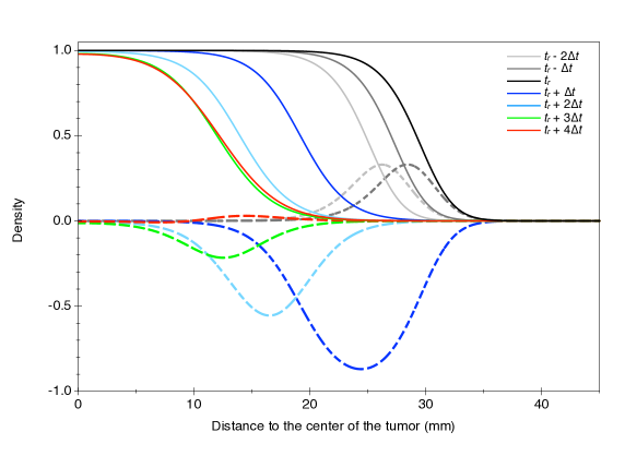
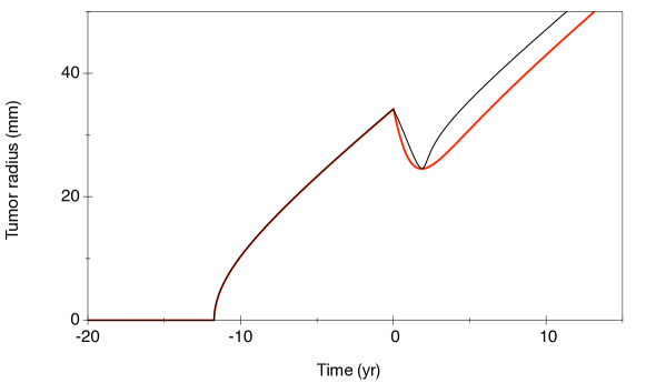
This is different from models with two populations (dammaged/undamaged cells) with constant death rates where the density is uniformly decreased. As shown later these models lead to a linear decrease just after RT (which is clearly not what is observed), while our model allows for an exponential-type decrease (more about the comparison in the Appendix).
Simple analytical considerations can give insights about the linear-versus-exponential early decrease of the radius. If we assume that at the time of RT the asymptotic regime is reached, then the profile of the cell density is a sigmoidal curve and the front propagates at a constant velocity:
| (9) |
At the time of RT (), the profile of the cell density then follows Murray (2002):
| (10) |
where the characteristic length is and is defined so that .
Since we are interested in the evolution of the radius, corresponding to a very low threshold of cell density () the profile is locally well described near by
| (11) |
Just after RT, the time during which the radius decreases before regrowth is short enough for us to neglect the effect of the diffusion on the shape of the front. In this case the cell density follows the equation:
| (12) | |||||
near the threshold where the saturation term can be neglected.
The solution to this equation for is:
| (13) |
So after RT the cell density close to the threshold (at large ), can be rewritten as:
| (14) |
Setting , one finds the evolution of the radius at the threshold:
| (15) |
If the death term is constant, then and the radius just after RT varies linearly with a constant velocity: . On the other hand, if is an exponential function, we obtain:
| (16) |
We can write this equation in a more simple way, by reintroducing the effective velocity (Eq 9) and defining being the radius of the tumor at the time of RT. After RT (for ) the equation of evolution of the tumor radius is:
| (17) |
This evolution is similar to a two-population model where a damaged one decreases exponentially at some characteristic time and amplitude and an undamaged one that still grows linearly at the asymptotic speed .
Finally we stress that this is only an approximate description aiming at capturing the gross features of the radius evolution but that in the following the exact Eq (4) is numerically solved.
3.2 Best fits
For each of our 43 patients, we performed the 5D minimization of the Eq (6) objective function; each one leads to a minimal value of the function (called ) for a set of parameters that represents the "best fit". Figure 2 shows the agreement between our best fit model and the data for a large number of patients with various medical follow-ups.
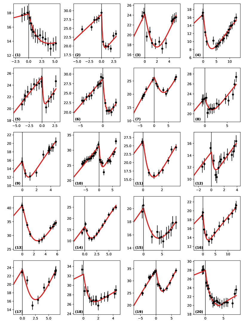
2 \switchcolumn
Our model allows to reproduce all the various cases in a very satisfactory way and although for space reasons we present results for 20 patients (the ones with the largest number of points) this is the case on all our 43 datasets (the 23 remaining fits are available in the Supplementary Material).
3.3 Tumor age
An original aspect of this work is that we consider the age of the tumor (defined with respect to RT time) as a free parameter, and we will now show that it is possible to get some information about this parameter.
Even when there is a substantial number of points before RT (which is rarely the case), one cannot simply extrapolate linearly back in time to determine the tumor birth date since there exists an invisible phase corresponding to the development of the tumor, but below the detection level and thus not detectable Gerin et al. (2012); Pallud et al. (2013). In order to put some constraint on the tumor age , we resort to the technique of the profile-likelihood (see e.g.. James (2007)) that works in the following way.
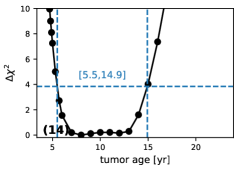
The tumor age is fixed at some value and a minimization over the 4 remaining parameters is performed, giving a value. The procedure is repeated for several values. Taking as zero point the lowest value, one can reconstruct the profile-likelihood of the tumor age, which can now be used to put a quantitative constraint on the parameter. Indeed it can be shown (e.g. James (1980)) that this function converges to a distribution with one degree of freedom so one can use its quantiles to get confidence level intervals. In particular one obtains a 95% confidence level intervals by thresholding the profile likelihood at 3.84.
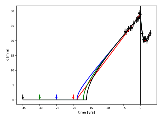
We have reconstructed the constraint on the tumor age (at RT) for all our selected 20 patients 444they are available as Supplementary Material and highlight some typical cases that show why the constraint depends crucially on the data on the patient follow-ups (Figure 2).
-
•
(a): patient (6): this is a case where there are many points before RT and few during the regrowth phase.
-
•
(b): patient (14) is the inverse, few points before RT but the regrowth is strongly sampled.
-
•
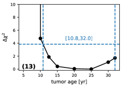
(c): Patient (13): no points before RT and a few during regrowth.
The corresponding profile-likelihoods are shown on Figure 3.
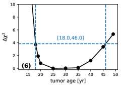
For patient (a) one obtains both a minimum age constraint (18 years) and a maximum one (46 years). The points before RT fix both the radius at RT and the slope. The latter essentially constrains the product through the asymptotic speed (). The invisible phase depends essentially on the proliferation rate and has a natural limit Gerin et al. (2012). Its duration cannot be smaller that the time at which the first point was measured. This fixes the tumor age lower limit. The upper limit comes from the fact that when the age increases, the proliferation rate is getting smaller. For small the radius evolution after the invisible phase is more and more curved which finally is in disagreement with the data near RT and our constraint on the linearity of the evolution at mm. This fixes the tumor age upper limit. Between those limits, several models, corresponding to several sets of parameters, fit equally well the data. This is illustrated on Figure 4 where we plotted the four models corresponding to the bottom points of Figure 3a (at 20, 25, 30 and 35 years) which all agree well with the data. One can see that the black model, the farthest from RT (35 years) has more curvature than the others and that the red one, with the smallest age (20) corresponds to a very brief invisible phase. In this case, the silent phase is close to its minimum compatible wit the data points for this patient.
Patient (14) does not have much constraint before RT (Figure 2) however the same type of constraint arises from the regrowth phase that still follows the asymptotic limit, so we still obtain a full range of valid tumor ages.
Finally, although patient (13) has no points before RT and has points only at the beginning of the regrowth phase, one can still put a lower limit on the tumor age through the full fitting of the five parameters model to the data. This demonstrates the potential of this method that can still put some minimum bound on the tumor age by exploiting the full data information.
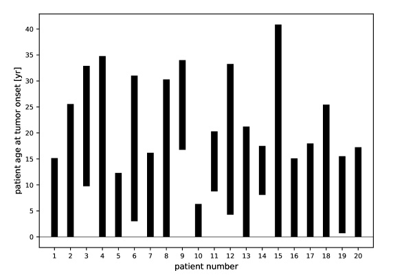
From the profile-likelihood reconstruction of all the 20 patients we can study the age of the patients at the birth of the tumors, which is calculated as the age of the patient at the RT minus the age of the tumor at RT. We show on Figure 5 all the 95% CL intervals obtained with this method. Although the constraints depend crucially on the data (size and sampling dates) they are consistent with a DLGG appearance at adolescence, as predicted in Gerin et al. (2012).
3.4 Tumor characteristics
As already pointed out, the tumor age is a parameter that is very different from the other ones: it is only an unknown of the problem, this is why we have treated it separately. The other four parameters () describe the DLGG evolution but, for a given tumor age, they are strongly correlated.
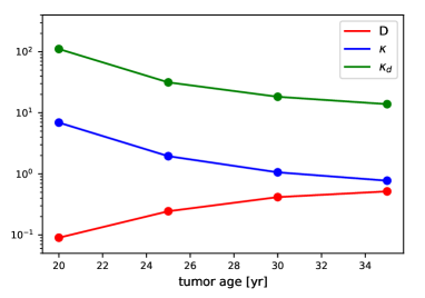
To illustrate it, let us consider again all the models corresponding to the “bottom points" of Figure 3a (). We show their values depending on the tumor age on Figure 6a. While all the models are essentially equivalent in terms of the parameters vary considerably (in a correlated way) prohibiting any interesting individual constraint.
Inspired by Eq (17), we propose to use instead the following parameters: and . We show on Figure 6b that they are indeed stable in the valid age range so that the variables are now uncorrelated.
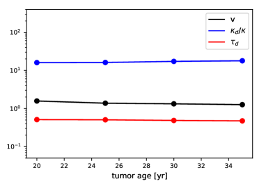
We then study if there are some common features among our patients. Figure 7 shows the histograms of the measured characteristics.
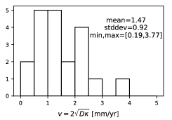


The measured velocities are consistent with DLGGs with values in the typical [1,4] range Mandonnet et al. (2008). The characteristics death rate times are about . The ratio between the death and proliferation rates after RT is large, typically above 5 but with a wide distribution that can go up to 40.
We can also check if there are some correlations between the evolution before and after RT. From the best fit models, we compute the following observables: ) the slope just before RT, the time at which the minimum is reached, the amplitude decrease at this point, and the time where the radius is the same than at RT during the regrowth phase.
On the dataset we measure the following correlation coefficients:
| (18) | |||||
From these expressions we expect some correlation between and , an anti-correlation between and through but moderate because of the logarithm, and a stronger one with , which is what is measured. We can conclude that our model reproduces correctly the correlations observed on data before and after RT.
4 Discussion
DLGG are tumors that always turn into a more aggressive form after years of indolent growth El-Hateer et al. (2009). They are also resistant to RT since they systematically recur after the end of the treatment. Modeling their dynamics, with and without treatment, can lead to a better understanding of their evolution and their resistance to treatments.
Here we complement a classical diffusion-proliferation model (that has already proved its usefulness for DLGG evolution) with a model of the RT effect, as a simple time-dependent and spatially structured death term. The spatial dependency of the death term means that cells at the border of the tumor are killed more than cells at the center of the tumor. The time dependency of the death term translates into a net proliferation term (proliferation minus death) that is time-dependent: before RT, the net proliferation is positive, then negative during a certain time interval after RT. When the death coefficient is smaller than the proliferation parameter , the net proliferation term is positive again and the tumor resumes its growth at the same rate as before RT.
The first qualitative feature that our model reproduces, without RT, is the fact that proliferating cells are situated at the border of the tumor. This spatial effect has been observed on human tissue from DLGG: by analyzing tissue samples from stereotaxic biopsies, it has been shown that cycling cells (or proliferating cells) are situated at the border of the tumor Gerin et al. (2013). Even if DLGG do not have a necrotic (and even hypoxic) center as higher grade gliomas, the cell density is still higher than normal. It is thus possible that some regions of sub-optimal oxygen concentration develop at the center of the tumor, reducing proliferation and triggering the transformation of cells into quiescent ones. We will see later that this spatial organization, that our model reproduces well, is crucial in the modeling of RT action.
Another important point is the modeling of the RT effect: although it is certainly a complicated effect that varies among patients, we argue that our choice of a time-dependent death rate is biologically realistic. Tumour irradiation induces both direct and indirect effects that could lead to tumor cell death. Direct effects are the result of radiation-induced DNA damages in cancer cells too important to be repaired (double strand breaks in the DNA molecules). But RT can also induce indirect damage to DNA (via reactive oxygen species), and to the tumour microenvironment such as vasculature. It can also trigger an immune response that can contribute to the tumor growth control Wang et al. (2018); Sia et al. (2020). Usually, damages cells try to repair the damages, and can even try to go through several mitoses before triggering their death. All of these process can take some time, and this is why the response to RT can be prolonged in time. We decide to model this delayed effect by defining a characteristic time in the death term. The choice of the exponential function for the death term is the simplest way to introduce a characteristic time. But it could also be justified in an other way: the linear quadratic model stipulates that the survival time is an exponential function of the dose received (for a review on the linear quadratic model, see McMahon (2018)). However, the efficacy of a given dose has been measured with cell culture in 2D. In a real tumor, it is possible that the efficacy of a dose depends on the microenvironment. It is a well-known fact that hypoxic cells (at the center of tumors) are more resistant to RT than normoxic cells Amberger-Murphy (2009). Actually, this constitutes an important limitation to the use of RT. So, for a given dose received, the radiation could have a smaller effect for cells close to the poor-oxygenated center than at the well-oxygenated border, leading to a larger survival rate. Just after RT, the more damaged cells begin to die, quiescent cells are now at the border and turn into proliferating ones and thus die also, but with a death rate smaller than the first layer. And so on, cells would die layer by layer, from the outside inwards. This process would justify our exponentially decreasing with time death rate. Biologically, this process is realistic: it has been actually observed in vitro and modeled with a cellular automaton for spheroids in Bruningk et al. (2020, 2019).
When compared to numerous high-quality clinical data (patients follow-up with tumor radius measurements for several time points), our time dependent death rate model, could reproduce the exponential shape visible on the experimental data: a sharp decline in a first time, followed by a slower decay, and an almost linear regrowth. With simple analytical considerations, we show that with a constant death term, the decrease of the radius can only be linear (at best) and cannot lead to any exponential-like decrease. For example, in our model of RT with edema, the early evolution is clearly linear Badoual et al. (2014).
We took care not to introduce too many parameters in out model, still allowing flexibility to describe all the data. The tumour evolution with RT is only described by 4 parameters, two being the natural evolution ones (proliferation and diffusion) and two for the RT effect (death rate and characteristic time). An original aspect of this work is that we also considered the (unknown) tumour age as a free parameter that could therefore be constrained by the data.
With this five-parameter model, the data of the temporal evolution of tumors radius for 43 patients were fitted automatically and give excellent results. We selected 20 patients with more than 10 data points (the fits for the other 23 patients are available in the Supplementary Material), and for each patient of this series, by scanning the possible ages of the tumor, from 0 to the patient age, we could infer the possible age range of the patient at the onset of the tumor. We find that the age at the onset of the tumor compatible with most of the patients is around 15 years-old. This finding confirms previous research Gerin et al. (2012), where, from the data of velocity and one measure of the tumor radius at a given time and going back in time with a model, the conclusion was that patients were most likely to be in their late teenage years at the onset of the tumor.
This age at the onset of the tumor depends on the initial conditions: if the simulation starts from a small clump of cells, the time needed to from that clump is not counted and the age of the tumor is underestimated. Moreover, the choice of the size of the clump would have been subjective. We chose to start the simulations from one cell. We also assumed that the proliferation and diffusion coefficients were constant all along the tumor evolution. This is a strong assumption that may not be correct. It is indeed possible that the first cell only proliferates, and form a small clump of cells before diffusion takes place. On the other hand, since we do not have any clue about what happened at the beginning of the evolution, and since even when discovered early, DLGG seem to grow the same way as larger tumors (associating proliferation and diffusion), we decided that the simplest way to choose the initial conditions was to start with one unique cell and the same proliferation and diffusion coefficient.
For the population of 20 selected patients, we also measured a RT characteristic time of around 1 year and a ratio of the maximal death coefficient to the proliferation coefficient always larger than 5. The fact that this ratio has a value larger than 1 is an important biological result: it means that just after RT, a large quantity of cells is killed just after RT and does not have time to go through any mitosis. In these cells, the damage due to RT may have been so important that the cells trigger the apoptosis program immediately, without even trying to perform a mitosis.
With the group of the 20 selected patients, we could also highlight good correlations between the velocity before RT, and both the gain of lifetime and (the maximum decrease of the radius). A simple analytical analysis allows to understand these correlations, that will be used, in a further work, to perform predictions.
no \appendixstart
Appendix A
In this Appendix we compare the evolution of the tumor radius obtained with our model, with a constant death rate model with two populations, inspired by Perez’ and Ribba’s work Ribba et al. (2012); Perez-García et al. (2015). In this model, RT damages a fraction of the cell population and this damaged population evolves differently from the undamaged one: the undamaged cell continue to proliferate and diffuse at the same rate as before, whereas the damaged population stops proliferating and die progressively (but still diffusing normally). A model of this type is interesting since it is biologically realistic and it accounts for the delay of the radius regrowth after RT. All the parameters are constant and beside the two parameters and describing the natural evolution of the tumor, two parameters are needed for RT, the fraction of the cell population that has been damaged, , and the death rate of this population, .
For , the equation describing the evolution of the cell population is the same as Eq (1):
For , two population are created: the damaged one, and the non damaged one : . After RT (:
for the non damaged population, and :
with .
This model can reproduce the regrowth delay after RT. However, as shown in Sect.3.1 the decrease of the radius is at best linear, which is as is clear from Figure 2, not in agreement with the clinical data, where a steep decrease is generally first observed followed by some milder phase. On Figure 8, the time of RT has been set to 0, and the RT parameters of the two models have been chosen so that the minimum of the radius evolution is the same. The linear decrease obtained with a two-population model after RT can be compared to the exponential decay with our one-population model. In the regrowth phase, the evolution of the radius with the two-population model displays a strong curvature reminiscent of the beginning of the visible radius evolution.
References
References
- Louis et al. (2007) Louis, D.N.; Ohgaki, H.; Wiestler, O.D.; Cavenee, W.K.; Burger, P.C.; Jouvet, A.; Scheithauer, B.W.; Kleihues, P. The 2007 WHO Classification of Tumours of the Central Nervous System. Acta Neuropathol. 2007, 114, 97–109.
- Louis et al. (2016) Louis, D.; Perry, A.; Reifenberger, G.; von Deimling, A.; Figarella-Branger, D.; Cavenee, W.; Ohgaki, H.; Wiestler, O.; Kleihues, P.; Ellison, D. The 2016 World Health Organization Classification of Tumors of the Central Nervous System: a summary. Acta Neuropathol. 2016, 131, 803–820.
- Marra et al. (2019) Marra, J.; Mendes, G.; Yoshinari, G.J.; da Silva Guimaraes, F.; Mazin, S.; de Oliveira, H. Survival after radiation therapy for high-grade glioma. Rep. Pract. Oncol. Radiother. 2019, 24, 35–40.
- Pallud et al. (2012) Pallud, J.; Llitjos, J.F.; Dhermain, F.; Varlet, P.; Dezamis, E.; Devaux, B.; Souillard-Scémama, R.; Sanai, N.; Koziak, M.; Page, P.; Schlienger, M.; Daumas-Duport, C.; Meder, J.F.; Oppenheim, C.; F.-X, R. Dynamic imaging response following radiation therapy predicts long-term outcomes for diffuse low-grade gliomas. Neuro Oncol 2012, 14, 1–10.
- Pallud and Mandonnet (2011) Pallud, J.; Mandonnet, E. Quantitative Approach of the Natural Course of Diffuse Low-Grade Gliomas. Tumors of the Central Nervous System, Volume 2, Springer 2011, pp. 163–172.
- Price (2010) Price, S.J. Advances in imaging low-grade gliomas. Adv. Tech. Stand. Neurosurg 2010, 35, 1–34.
- Kelly et al. (1987) Kelly, P.J.; Daumas-Duport, C.; Kispert, D.B.; Kall, B.A.; Scheithauer, W.; Illig, J. Imaging-based stereotaxic serial biopsies in untreated intracranial glial neaplasms. J Neurosurg 1987, 66, 865–874.
- Pallud et al. (2010a) Pallud, J.; Varlet, P.; Devaux, B.; Geha, S.; Badoual, M.; Deroulers, C.; Page, P.; Dezamis, E.; Daumas-Duport, C.; Roux, F.X. Diffuse low-grade oligodendrogliomas extend beyond MRI-defined abnormalities. Neurology 2010, 74, 1724–1731.
- Pallud et al. (2010b) Pallud, J.; Fontaine, D.; Duffau, H.; Mandonnet, E.; Sanai, N.; Taillandier, L.; Peruzzi, P.; Guillevin, R.; Bauchet, L.; Bernier, V.; Baron, M.H.; Guyotat, J.; Capelle, L. Natural history of incidental WHO grade II gliomas. Annals of Neurology 2010, 68, 727–33.
- Ricard et al. (2007) Ricard, D.; Kaloshi, G.; Amiel-Benouaich, A.; Lejeune, J.; Marie, Y.; Mandonnet, E.; Kujas, M.; Mokhtari, K.; Taillibert, S.; Laigle-Donadey, F.; Carpentier, A.; Omuro, A.; Capelle, L.; Duffau, H.; Cornu, P.; Guillevin, R.; Sanson, M.; Hoang-Xuan, K.; Delattre, J. Dynamic history of low-grade gliomas before and after temozolomide treatment. Ann. Neurol 2007, 61, 484–490.
- Peyre et al. (2010) Peyre, M.; Cartalat-Carel, S.; Meyronet, D.; Ricard, D.; Jouvet, A.; Pallud, J.; Mokhtari, K.; Guyotat, J.; Jouanneau, E.; Sunyach, M.; Frappaz, D.; Honnorat, J.; Ducray, F. Prolonged response without prolonged chemotherapy: a lesson from PCV chemotherapy in low-grade gliomas. Neuro. Oncol 2010, 12, 1078–1082.
- Mandonnet et al. (2009) Mandonnet, E.; Pallud, J.; Fontaine, D.; Taillandier, L.; Bauchet, L.; Peruzzi, P.; Guyotat, J.; Bernier, V.; Baron, M.H.; Duffau, H.; Capelle, L. Inter- and intrapatients comparison of WHO grade II glioma kinetics before and after surgical resection. Neurosurgical Review 2009, 33, 91–96.
- Prabhu et al. (2010) Prabhu, V.C.; Khaldi, A.; Barton, K.P.; Melian, E.; Schneck, M.J.; Primeau, M.J.; Lee, J.M. Management of diffuse low-grade cerebral gliomas. Neurologic Clinics 2010, 28, 1037–1059.
- Bobek-Billewicz et al. (2014) Bobek-Billewicz, B.; Stasik-Pres, G.; Hebda, A.; Majchrzak, K.; Kaspera, W.; Jurkowski, M. Anaplastic transformation of low-grade gliomas (WHO II) on magnetic resonance imaging. Folia Neuropathol. 2014, 52, 128–140.
- van den Bent et al. (2005) van den Bent, M.; Afra, D.; de Witte, O.; Ben Hassel, M.; Schraub, S.; Hoang-Xuan, K.; Malmström, P.; Collette, L.; Piérart, M.; Mirimanoff, R.; Karim, A.; Radiotherapy, E.; Groups, B.T.; the UK Medical Research Council. Long-term efficacy of early versus delayed radiotherapy for low-grade astrocytoma and oligodendroglioma in adults: the EORTC 22845 randomised trial. Lancet 2005, 366, 985–990.
- Dufour et al. (2018) Dufour, A.; Gontran, E.; Deroulers, C.; Varlet, P.; Pallud, J.; Grammaticos, B.; Badoual, M. Modeling the dynamics of oligodendrocyte precursor cells and the genesis of gliomas. Cancer 2018, 14, e1005977.
- Gerin et al. (2012) Gerin, C.; Pallud, J.; Grammaticos, B.; Mandonnet, E.; Deroulers, C.; Varlet, P.; Capelle, L.; Taillandier, L.; Bauchet, L.; Duffau, H.; Badoual, M. Improving the time-machine: estimating date of birth of grade II gliomas. Cell. Prolif 2012, 45, 76–90.
- Ribba et al. (2012) Ribba, B.; Kaloshi, G.; Peyre, M.; Ricard, D.; Calvez, V.; Tod, M.; Cajavec-Bernard, B.; Idbaih, A.; Psimaras, D.; Dainese, L.; Pallud, J.; Cartalat-Carel, S.; Delattre, J.Y.; Honnorat, J.; Grenier, E.; Ducray, F. A tumor growth inhibition model for low-grade glioma treated with chemotherapy or radiotherapy. Clin. Cancer Res 2012, 18, 5071–5080.
- Badoual et al. (2014) Badoual, M.; Gerin, C.; Deroulers, C.; Grammaticos, B.; Llitjos, J.; Oppenheim, C.; Varlet, P.; Pallud, J. Oedema-based model for diffuse low-grade gliomas: application to clinical cases under radiotherapy. Cell. Prolif. 2014, 47, 369–380.
- Perez-García et al. (2015) Perez-García, V.; Bogdanska, M.; Martínez-Gonzalez, A.; Belmonte-Beitia, J.; Schucht, P.; Perez-Romasanta, L. Delay effects in the response of low-grade gliomas to radiotherapy: a mathematical model and its therapeutical implications. Math. Med. Biol. 2015, 32, 307–329.
- Galochkina et al. (2015) Galochkina, T.; Bratus, A.; Perez-Garcia, V. Optimal radiation fractionation for low-grade gliomas: Insights from a mathematical model. Math. Biosci. 2015, 267, 1–9.
- Budia et al. (2019) Budia, I.; Alvarez-Arenas, A.; Woolley, T.; Calvo, G.; Belmonte-Beitia, J. Radiation protraction schedules for low-grade gliomas: a comparison between different mathematical models. J. R. Soc. Interface 2019, 16, 20190665.
- Bogdanska et al. (2017) Bogdanska, M.; Bodnar, M.; Piotrowska, M.; Murek, M.; Schucht, P.; Beck, J.; Martinez-Gonzalez, A.; Perez-Garcia, V. A mathematical model describes the malignant transformation of low grade gliomas: Prognostic implications. PLoS One 2017, 12, e0179999.
- Harpold et al. (2007) Harpold, H.L.; Jr, E.C.A.; Swanson, K.R. The evolution of mathematical modeling of glioma proliferation and invasion. J. Neuropathol. Exp. Neurol 2007, 1, 1–9.
- Badoual et al. (2010) Badoual, M.; Deroulers, C.; Aubert, M.; Grammaticos, B. Modelling intercellular communication and its effect on tumour invasion. Phys. Biol. 2010, 7, 046013.
- Corwin et al. (2013) Corwin, D.; Holdsworth, C.; Rockne, R.; Trister, A.; Mrugala, M.; Rockhill, J.; Stewart, R.; Phillips, M.; Swanson, K. Toward patient-specific, biologically optimized radiation therapy plans for the treatment of glioblastoma. PLoS One 2013, 8, e79115.
- Unkelbach et al. (2014) Unkelbach, J.; Menze, B.; Konukoglu, E.; Dittmann, F.; Le, M.; Ayache, N.; Shih, H. Radiotherapy planning for glioblastoma based on a tumor growth model: improving target volume delineation. Phys. Med. Biol. 2014, 59, 747–770.
- Amelot et al. (2017) Amelot, A.; Deroulers, C.; Badoual, M.; Polivka, M.; Adle-Biassette, H.; Houdart, E.; Carpentier, A.; Froelich, S.; Mandonnet, E. Surgical Decision Making From Image-Based Biophysical Modeling of Glioblastoma: Not Ready for Primetime. Neurosurgery 2017, 80, 793–799.
- Mandonnet et al. (2003) Mandonnet, E.; Delattre, J.Y.; Tanguy, M.L.; Swanson, K.R.; Carpentier, A.F.; Duffau, H.; Cornu, P.; Van Effenterre, R.; E. C. Alvord, J.; Capelle, L. Continuous growth of mean tumor diameter in a subset of grade II gliomas. Annals of Neurology 2003, 53, 524–528.
- Pallud et al. (2006) Pallud, J.; Mandonnet, E.; Duffau, H.; Kujas, M.; Guillevin, R.; Galanaud, D.; Taillandier, L.; Capelle, L. Prognostic value of initial magnetic resonance imaging growth rates for World Health Organization grade II gliomas. Annals of Neurology 2006, 60, 380–383.
- Rockne et al. (2010) Rockne, R.; Rockhill, J.K.; Mrugala, M.; Spence, A.M.; Kalet, I.; Hendrickson, K.; Lai, A.; Cloughesy, T.; Alvord, E.C.J.; Swanson, K.R. Predicting the efficacy of radiotherapy in individual glioblastoma patients in vivo: a mathematical modelling approach. Phys. Med. Biol 2010, 55, 3271–3285.
- Henares-Molina et al. (2017) Henares-Molina, A.; Benzekry, S.; Lara, P.; Garcia-Rojo, M.; Perez-Garcia, V.; Martinez-Gonzalez, A. Non-standard radiotherapy fractionations delay the time to malignant transformation of low-grade gliomas. PLoS One 2017, 12, e0178552.
- Hansen and Ostermeier (2001) Hansen, N.; Ostermeier, A. Completely Derandomized Self-Adaptation in Evolution Strategies. Evolutionary Computation 2001, 9, 159–195, [https://direct.mit.edu/evco/article-pdf/9/2/159/1493523/106365601750190398.pdf]. doi:\changeurlcolorblack10.1162/106365601750190398.
- Murray (2002) Murray, J.D. Mathematical biology. II: Spatial models and biomedical applications, 3rd ed.; Springer-Verlag : Berlin, 2002.
- Pallud et al. (2013) Pallud, J.; Capelle, L.; Taillandier, L.; Badoual, M.; Duffau, H.; Mandonnet, E. The silent phase of diffuse low-grade gliomas. Is it when we missed the action? Acta Neurochir. 2013, 155, 2237–2242.
- James (2007) James, F. Statistical Methods in Experimental Physics; World Scientific, 2007.
- James (1980) James, F. Interpretation of the shape of the likelihood function around its minimum. Computer Physics Communications 1980, 20, 29–35. doi:\changeurlcolorblack10.1016/0010-4655(80)90103-4.
- Mandonnet et al. (2008) Mandonnet, E.; Pallud, J.; Clatz, O.; Taillandier, L.; Konukoglu, E.; Duffau, H.; Capelle, L. Computational modeling of the WHO grade II glioma dynamics: principles and applications to management paradigm. Neurosurg. Rev 2008, 31, 263–269.
- El-Hateer et al. (2009) El-Hateer, H.; Souhami, L.; Roberge, D.; Maestro, R.D.; Leblanc, R.; Eldebawy, E.; Muanza, T.; Melançon, D.; Kavan, P.; Guiot, M.C. Low-grade oligodendroglioma: an indolent but incurable disease? J. Neurosurg 2009, 111, 265–271.
- Gerin et al. (2013) Gerin, C.; Pallud, J.; Deroulers, C.; Varlet, P.; Oppenheim, C.; Roux, F.X.; Chrétien, F.; Grammaticos, B.; Badoual, M. Quantitative characterization of the imaging limits of diffuse low-grade oligodendrogliomas. Neuro-Oncology 2013, p. in press.
- Wang et al. (2018) Wang, J.; Wang, H.; Qian, H. Biological effects of radiation on cancer cells. Mil. Med. Res. 2018, 5, 20.
- Sia et al. (2020) Sia, J.; Szmyd, R.; Hau, E.; Gee, H. Molecular Mechanisms of Radiation-Induced Cancer Cell Death: A Primer. Front. Cell. Dev. Biol. 2020, 8, 41.
- McMahon (2018) McMahon, S. The linear quadratic model: usage, interpretation and challenges. Phys. Med. Biol. 2018, 64, 01TR01.
- Amberger-Murphy (2009) Amberger-Murphy, V. Hypoxia helps glioma to fight therapy. Curr Cancer Drug Targets 2009, 9, 381–390.
- Bruningk et al. (2020) Bruningk, S.; Rivens, I.; Box, C.; Oelfke, U.; G., T.H. 3D tumour spheroids for the prediction of the effects of radiation and hyperthermia treatments. Sci. Rep. 2020, 10, 1653.
- Bruningk et al. (2019) Bruningk, S.; Ziegenhein, P.; Rivens, I.; Oelfke, U.; Haar, G. A cellular automaton model for spheroid response to radiation and hyperthermia treatments. Sci. Rep. 2019, 9, 17674.