GPDs of hadrons and elastic pion-nucleon scattering

Abstract

The pion structure is represented by generalized parton distribution functions (GPDs). The momentum transfer dependence of GPDs of the pion was obtained on the basis of the form of GPDs of the nucleon in the framework of the high energy generalized structure (HEGS) model. To this end, different forms of PDFs of the pion of various Collaborations were examined with taking into account the available experimental data on the pion form factors. As a result, the electromagnetic and gravitomagnetic form factors of the pion were calculated. They were used in the framework of the HEGS model with the electromagnetic and gravitomagnetic form factors of the proton for describing pion-nucleon elastic scattering in a wide energy and momentum transfer region with a minimum of fitting parameters. The properties of the obtained scattering amplitude were analyzed.

I Introduction

The study of the particle structure is one of the old and long-standing problems in modern physics. The main step was made by introducing the parton picture of hadrons. Now many collaborations have obtained some forms of the parton distribution functions (PDF) using the recent data obtained at HERA and LHC in deep inelastic scattering. Besides this main point of the modern picture of the hadron structure, which depends only on the Bjorken longitudinal variable $x$, there were introduced a number of other more complicated structure functions, for example, the generalized parton distribution functions (GPDs) (which depend on $\ x$, momentum transfer $t$ and the skewness parameter $\xi$), transverse momentum distributions (TMDs) functions (which depend on $x$, inner momentum transfer $k$ and skewness parameters $\xi$) and many others. Now we have more generalized parton distributions which depend on different variables $GTMDs(x,\vec{k},\xi,\vec{\Delta)}$, generalized transverse momentum dependent distributions of partons Meis-08 ; Lorce-13 ; Burk-15 . They are parameterized by the unintegrated off-diagonal quark-quark correlator depending on the three-momentum $\vec{k}$ of the quark and on the four-momentum, which is transferred by the probe to the hadron. Taking $\Delta=0$, we can obtain $TMD(x,\vec{k})$ the transverse momentum-dependent parton distribution. In another way, after integration over $\vec{k}$ we obtain $GPDs(x,\xi,\Delta)$, generalized parton distributions.

The remarkable property of $GPDs$ is that the integration of different momenta of GPDs over $x$ gives us different hadron form factors Mil94 ; Ji97 ; R97 . The $x$ dependence of $GPDs$ is determined, in most part, by the standard PDFs, which are obtained by many Collaborations from the analysis of deep-inelastic processes. Specific reactions can be related with different form factors. For example, strong hadron-hadron scattering can be proportional to the gravitomagnetic form factor or the matter distribution of hadrons, and the Compton scattering is described by the Compton form factors. Hence, the generalized parton distributions reveal themselves as a bridge between the data on the inelastic reaction and the recent data on the elastic hadron-hadron cross section. Many different forms of the momentum transfer dependence of GPDs were proposed. In the quark diquark model Liuti1 the form of GPDs consists of three parts - PDFs, function distribution and the Regge-like function. In other works (see e.g. Kroll04 ), the description of the $t$-dependence of GPDs was developed in a more complicated picture using the polynomial forms with respect to $x$.

Note that functions like GPDs(x,t, $\xi=0$) were already used in the old ”Valon” model proposed by Sanielevici and Valin in 1986 San-Val . In that model, the hadron elastic form factor was obtained by the integration function $L(x)G(x,t)$ where $L(x)$ corresponds to the parton function and $G(x,t)$ corresponds to an additional function which depends on the momentum transfer and $x$. In modern language, this exactly corresponds to GPDs. The recent results from the LHC gave plenty of new information about the elastic and deep-inelastic processes, which raised new questions in the study of the structure of hadrons.

In the paper, we analyze the hadrons structure, which is presented by the GPDs of hadrons. In Sec. II, the momentum transfer dependence of GPDs of hadrons obtained in the framework of the high energy generalized structure (HEGS) model is discussed. It is very important to check the obtained $t$-dependence of GPDs, as it determined the $t$-dependence of the gravitomagnetic form factor of nucleons, which in turn impact on momentum transfer dependence of the differential cross sections. As an example, in Sec. III we calculated by integration other Mellin moments of GPDs which give us the corresponding Compton form factors and transition magnetic form factor. Comparing the corresponding cross sections determined by Compton form factors and transition magnetic form factor with the existing experimental data gives us additional support of the obtained $t$-dependence of GPDs. In Se. IV, a short review of the results of the HEGS model for the nucleon structure and nucleon-nucleon scattering is presented. In Sec. V, the GPDs of the pion are determined, and on their basis the electromagnetic and gravitomagnetic pion form factors are calculated. In Sec. VI, the obtained nucleon and pion form factors are used in the framework of the HEGS model for pion-nucleon elastic scattering. The conclusion is presented in the final section.

II Momentum transfer dependence of GPDs of nucleon

In ST-PRDGPD , the standard Gaussian ansatz of the $t$-dependence of GPDs is chosen in a simple form

$${\cal{H}}^{q}(x,t)\ =q(x)\ exp[a_{+}\ f(x)\ t],$$ (1)

with $f(x)=(1-x)^{2}/x^{\beta}.$ The isotopic invariance can be used to relate the proton and neutron GPDs. The complex analysis of the corresponding description of the electromagnetic form factors of the proton and neutron by different PDFs sets (24 cases) was carried out in GPD-PRD14 . These PDFs include the leading order (LO), next leading order (NLO) and next-next leading order (NNLO) determination of the parton distribution functions. They used different forms of the $x$ dependence of PDFs. A slightly complicated form of GPDs was taken into acount in comparison with the equation used in ST-PRDGPD , but it is the simplest one as compared to other works (for example, DK-13 , where $f(x,t)_{q}$ was chosen in the form with different $x$ dependence, six parameters control the small $x$ behavior of these functions, whereas their behavior at large $x$ is controlled other six parameters. Note, that in Yuan-04 , it was shown that at large $x\rightarrow 1$ and momentum transfer the behavior of GPDs requires a larger power of $(1-x)^{b}$ in the $t$-dependent exponent.

$${\cal{H}}_{u}(x,t)\ = q_{u}(x)\ e^{2a_{H}f_{u}(x)\ t};\ \ \$$ (2)

$${\cal{H}}_{d}(x,t)\ = q_{d}(x)\ e^{2a_{H}f_{d}(x)\ t};$$

$${\cal{E}}_{u}(x,t)\ = q_{u}(x)(1-x)^{\gamma_{u}}\ e^{2a_{E}\ f_{u}(x)t};\ \ \$$ (3)

$${\cal{E}}_{d}(x,t)\ = q_{d}(x)(1-x)^{\gamma_{d}}\ e^{2a_{E}f_{d}(x)t},$$

where

$$f_{u}(x)=\frac{(1-x)^{2+\epsilon_{u}}}{(x_{0}+x)^{m}},$$

$$f_{d}(x)=(1+\epsilon_{0})\frac{(1-x)^{2+\epsilon_{d}}}{(x_{0}+x)^{m}}.$$

with $a_{H},\gamma,\epsilon_{i},x_{0},m$ being the parameters determined from the analysis of the existing experimental data of the electomagnetic form factors.

On the basis of our GPDs with PDFs ABM12 ABM12 , we calculated the hadron form factors by numerical integration and then by fitting these integral results by the standard dipole form with some additional parameters

$$F_{1}(t) = (4m_{p}-\mu t)/(4m_{p}-t)$$

$$1/(1+q/a_{1}+q^{2}/a_{2}^{2}+q^{3}/a_{3}^{3})^{2}$$

where $m_{p}$ is the proton mass and $a_{i}$ are free parameters. That is slightly different from the standard dipole form of two additional terms with small sizes of the coefficients. The matter form factor

$$A(t)= \int^{1}_{0}x\ dx$$

$$[q_{u}(x)e^{2\alpha_{H}f)_{u}(x\ t}+q_{d}(x)e^{2\alpha_{H}f_{d}(x)\ t}]$$

is fitted by the simple dipole form

$$A(t)=\Lambda^{4}/(\Lambda^{2}-t)^{2}$$

where $\Lambda$ is a free parameter, which equal $1.6$ GeV² for the proton case. These form factors will be used in our model of the proton-proton and proton-antiproton elastic scattering and further in one of the vertices of pion-nucleon elastic scattering.

III Compton and magnetic transition form factors

It is very important to check the obtained $t$-dependence of GPDs, as it determined the $t$-dependence of the gravitomagnetic form factor of nucleons, which in turn impact on momentum transfer dependence of the differential cross sections. Let us calculate the moments of GPDs with inverse power of $x$. This gives us the Compton form factors $R_{V}((t)$, $R_{T}(t)$. Using the obtained form factors, the reaction of the real Compton scattering can be calculated CompFF . For $H^{q}(x,t)$, $E^{q}(x,t)$ with PDFs from the work Khang-16 , which was chosen on the basis of the analysis carried out in GPD-PRD14 and with the parameters obtained in our fitting procedure of describing the proton and neutron electromagnetic form factors in GPD-PRD14 . The form factors $R_{i}$ are determined

$$R_{i}(t)=\sum_{q}e^{2}_{q}\int_{0}^{1}\frac{dx}{x}{\cal{F}}j_{q}(x,\xi=0,t),$$ (6)

where ${\cal{F}}j_{q}$ are equal to $H_{q}$, $E_{q}$ and $\tilde{H}_{q}$ and give the form factors $R_{V}(t)$, $R_{T}(t)$, $R_{A}(t)$, respectively.

In the present work for $\tilde{H}^{q}(x,t)$ we take $\Delta q$ in the form Khang-16 for NNLO $Q_{0}=2$ GeV²

$$x\Delta_{q}(x,Q_{0})=N_{q}\eta_{q}x^{a_{q}}(1-x)^{b_{q}}(1+c_{q}x).$$ (7)

Assuming $SU(3)$ flavor symmetry of $\Delta\bar{q}$, the coefficient $N_{q}$ is determined as

$$\frac{1}{N_{q}}=(1+c_{q}\frac{a_{q}}{1+a_{q}+b_{q}})\ B(a_{q},b_{q}+1),$$ (8)

where $\ B(a_{q},b_{q}+1)$ is determined by

$$B(a,b)=\frac{\Gamma(a)\Gamma(b)}{\Gamma(a+b)}=\int_{0}^{1}t^{a-1}(1-t)^{b-1}dt.$$ (9)

The results of our calculations of the Compton form factors are shown in Fig. 1(a,b). The form factors $R_{V}(t)$ and $R_{T}(t)$ have a similar momentum transfer dependence but essentially differ in size. On the contrary, the axial form factor $R_{A}$ has an essentially different $t$ dependence. The calculations of $R_{i}$ on the whole, correspond to the calculations of DK-13 .

The differential cross section of the real Compton scattering can be written as DK-13

$$\frac{d\sigma}{dt}= \frac{\pi\alpha^{2}_{em}}{s^{2}}\frac{(s-u)^{2}}{-us}$$

$$[R_{V}^{2}(t)\ -\ \frac{t}{4m^{2}}R^{2}_{T}(t)+\frac{t^{2}}{(s-u)^{2}}R^{2}_{A}(t)],$$

where $R_{V}((t)$, $R_{T}(t)$, $R_{A}(t)$ are the form factors given by the $1/x$ moments of the corresponding GPDs $H^{q}(x,t)$, $E^{q}(x,t)$, $\tilde{H}^{q}(x,t)$ .

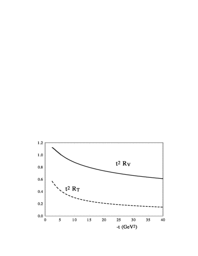
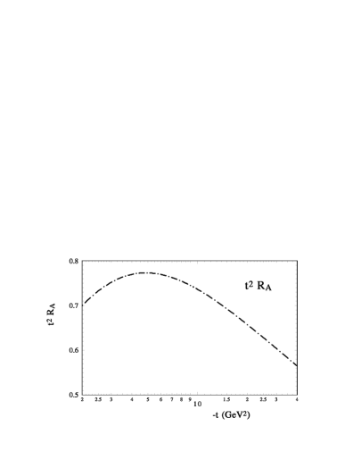
Figure 1: The Compton form factors a) [top] $t^{2}R_{V}(t)$ and $t^{2}R_{T}(t)$; b)[bottom] , $t^{2}R_{A}(t)$.

The results for the cross sections are presented in Fig.2. Except for very large angles at low energies the coincidence with experimental data is sufficiently good.

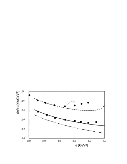
Figure 2: The differential Compton cross sections (the lines are our calculations at $s=8.9$ GeV², $s=10.92$ GeV² and $s=20$ GeV², the data points are for $s=8.9$ GeV² (circles)dt-Cmpt ; $s=10.92$ GeV² (squares) dt-Cmpt .

To check the obtained momentum dependence of the spin-dependent part of GPDs $E_{u,d}(x,\xi=0,t)$, we can calculate the magnetic transition form factor which is determined by the difference of $E_{u}(x,\xi=0,t)$ and $E_{d}(x,\xi=0,t)$. For the magnetic $N\rightarrow\Delta$ transition form factor $G^{*}_{M}(t)$, in the large $N_{c}$ limit, the relevant $GPD_{N\Delta}$ can be expressed in terms of the isovector GPD yielding the sum rule Guidal

$$G^{*}_{M}(t)= \frac{G^{*}_{M}(t=0)}{k_{v}}$$ (11)

$$\int_{-1}^{1}dx(E_{u}(x,\xi,t)-E_{d}(x,\xi,t))$$

where $k_{v}=k_{p}-k_{n}=3.70$.

Figure 3: The transition magnetic form factors $G^{*}_{M}(Q^{2})/(3G_{d})$ (line- our calculations, points are the experimental data ff-Gtr ).

The results of our calculations, based on eqs. (2) and (3), are presented in Fig.3. The experimental data exist up to $-t=8$ GeV² and our results show a sufficiently good coincidence with experimental data. It is confirmed that the form of the momentum transfer dependence of $E(x,\xi,t)$ determined in our model is correct.

IV Hadron form factors and elastic nucleon-nucleon scattering

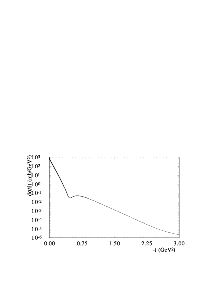
Figure 4: a) [top] The HEGS model calculations of the differential cross sections of elastic scattering of proton-proton (hard line) and proton-antiproton (dashed line) at $\sqrt{s}=52.2$ GeV, ( circles, quires, triangles up and triangles down - Rub19am ; Adam19 ; Schiz19 ; Aker19 ; Cul19 ; Rub19 ; Bri19 )
                                    b) [bottom] $pp$ elastic cross sections at $\sqrt{s}=13$ TeV (line - the HEGS model calculations, points - the data T66 ; T67 ).

In the framework of the high energy generalized structure (HEGS) model of elastic nucleon-nucleon scattering both hadron electromagnetic and gravitomagnetic form factors were used. This allows us to build a model with a minimum number of fitting parameters HEGS0 ; HEGS1 ; NP-hP .

The Born term of the elastic hadron amplitude can now be written as

$$F_{h}^{Born}(s,t) =h_{1}F_{1}^{2}(t)F_{a}(s,t)(1+r_{1}/\hat{s}^{0.5})$$ (12)

$$+ h_{2}\ A^{2}(t)\ F_{b}(s,t)\$$

$$\pm h_{odd}\ A^{2}(t)F_{b}(s,t)\ (1+r_{2}/\hat{s}^{0.5}),$$

where $F_{1}(t)$ is the electromagnetic proton form factor, which represents charge distribution in the proton, and $A(t)$ is the gravitation form factor which represents the matter distribution in the proton; hence, both (electromagnetic and gravitomagnetic) form factors are used. The parameters are determined in HEGS1 where $F_{a}(s,t)$ and $F_{b}(s,t)$ have the standard Regge form:

$$F_{a}(s,t)\ =\hat{s}^{\epsilon}\ e^{B(\hat{s})\ t};\ F_{b}(s,t)\ =\hat{s}^{\epsilon}\ e^{B(\hat{s})/4\ t},$$ (13)

where $\hat{s}=s\ e^{-i\pi/2}/s_{0}$ ; $s_{0}=4m_{p}^{2}\ {\rm(GeV^{2})}$, and $h_{odd}=ih_{3}t/(1-r_{0}^{2}t)$. The intercept $1+\epsilon=1.11$ was chosen from the data of different reactions and was fixed by the same size for all terms of the scattering amplitude. The slope of the scattering amplitude has the standard logarithmic dependence on the energy $B(s)=\alpha^{\prime}\ ln(\hat{s})$ with $\alpha^{\prime}=0.24$ GeV^-2 and with some small additional term HEGS1 , which reflects the small non-linear behavior of $\alpha^{\prime}$ Sel-Df16 . The final elastic hadron scattering amplitude is obtained after unitarization of the Born term by the standard eikonal representation. The model is very simple from the viewpoint of the number of fitting parameters and functions. There are no any artificial functions or any cuts which bound the separate parts of the amplitude by some region of momentum transfer.

In the framework of the model, the description of experimental data was obtained simultaneously at the large momentum transfer and in the Coulomb-hadron region, using the CNI phase selmp1 ; Selphase , in the energy range from $\sqrt{s}=9$ GeV up to LHC energies. In the basic form of the HEGS model $3416$ experimental points were included in our analysis in the energy region $9.8$ GeV $\leq\sqrt{s}\leq 8.$ TeV and in the region of momentum transfer $0.000375\leq|t|\leq 15$ GeV². The experimental data of proton-proton and proton-antiproton elastic scattering are included in 92 separate sets of 32 experiments, including recent data of the TOTEM Collaboration at $\sqrt{s}=8$ TeV. The whole Coulomb-hadron interference region, where the experimental errors are remarkably small, was included in our examination of experimental data. Our model of the GPDs leads to a good description of the proton and neutron electromagnetic form factors and their elastic scattering simultaneously. It allows one to find some new features in the differential cross section of $pp$-scattering in the unique experimental data of the TOTEM collaboration at $\sqrt{s}=13$ TeV (small oscillations Sel-PL19 and anomalous behavior at small momentum transfer anom13-20 ). The inclusion of the spin-flip parts of the scattering amplitude allows one to describe the low energy experimental polarization data of the $pp$ elastic scattering Symmetry , which are shown in the corresponding figures in Symmetry .

Figure 4(a) represents the description at $\sqrt{s}=52.8$ GeV and Figure 4(b) shows the model calculations for $\sqrt{s}=13$ TeV, which coincide well with the recent experimental data of the TOTEM Collaboration T66 ; T67 .

V GPDs of pion

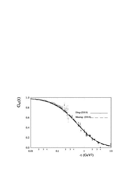
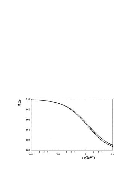
Figure 5: a) [top] The electromagnetic form factor of the $\pi$-meson (hard and dashed curves - our calculations with PDF Mez16 and and RayT , respectively; the circles and squares - the experimental data ff1 ; ff2 ; ff3 ; ff4 ; ff5 ; ff6 )
b) [bottom] the gravitomagnetic form factor of the pion with the normalization $A_{Gr}(t=0)=1$ (the hard and dashed curves - our calculation with the PDF Mez16 and RayT , respectively); long-dashed and tiny-dashed curves - the fits of our integral calculations by a simple monopole form.

The pion structure in some sense is simpler than the nucleon structure. In the nucleon there are 3 constituent quarks that can create different configurations, for example, such as ”Mercedes star” or a linear structure with a quark at one end and a di-quark at the other. These configurations can lead to different results for hadron interactions, for example, the Odderon-hadron coupling. For a meson we have only two quark states

$$|\pi>=|q\bar{q}>+|q\bar{q}\ q\bar{q}>+|q\bar{q}\ g>......$$

It is needed to note that the standard definition of the pion form factor through the matrix elements of the electromagnetic vector current

$$V_{\mu}(x)=e_{u}\bar{u}(x)\gamma_{\mu}u(x)-e_{d}\bar{d}(x)\gamma_{\mu}d(x),$$ (14)

gives

$$\langle\pi^{+}(\vec{p^{{}^{\prime}}})|V_{\mu}(0)|\pi^{+}(\vec{p})\rangle=(p_{\mu}^{{}^{\prime}}+p_{\mu})F_{\pi}(Q^{2}),$$ (15)

with $Q^{2}=-q^{2}$ and $F_{\pi}(Q^{2})$ being the space-like form factor of the pion ETM . It is related with the separate quark contributions

$$F_{\pi}(t)=e^{u}\ F_{\pi}^{u}-e^{d}\ F_{\pi}^{d}.$$ (16)

For the definition of the electromagnetic form factor of the pion there are many different approximations beginning with the standard monopole form

$$F_{\pi}=\Lambda^{2}/(\Lambda^{2}-t),$$ (17)

(with $\Lambda$ as a free parameter determined from experimental data), including the Regge exponential form

$$F_{\pi}=y^{-\alpha_{\pi}(t)}\frac{e^{t-m_{\pi}^{2}}}{\Lambda^{2}}$$

and monopole form with polynomial form of $t$ dependence Mez-14

$$F_{\pi}(t=M^{2}z)=\frac{1}{1+0.44z+0.06z^{2}+0.00033z^{3}}.$$

and in complicated form of $t$ dependence Meln03

$$F_{\pi}(Q^{2})=\frac{1}{1+Q^{2}/m_{\rho}^{2}}(\frac{1+c_{1}Z+c_{2}Z^{2}}{1+c_{1}Z+c_{2}Z^{2}+c_{3}Z^{3}}),$$

where $Z=Log(1+Q^{2}/\Lambda^{2})$ and $\Lambda$ is the QCD scale parameter. Such a form is similar to that proposed in Watanabe within a dispersion relation analysis; however, the presented form uses two additional parameters and takes a rather large value of $\Lambda=1$ GeV.

For the pion Generalized parton distribution we have the standard definition through the matrix element, for example Mez-14

$$H^{q}_{\pi}(x,t,\xi)=\frac{1}{2}\int\frac{dz^{-}}{2\pi}e^{ixP^{+}z^{-}}$$ (18)

$$\langle\pi,P+\frac{\Delta}{2}|\bar{q}(-\frac{z}{2})\gamma^{+}[-\frac{z}{2};\frac{z}{2}]q(\frac{z}{2})|\pi,P-\frac{\Delta}{2}\rangle_{z^{+}=0,x_{\perp}=0},$$

with the skewness $\xi=-\Delta^{+}/(2P^{+})$ and the momentum transfer $t=-\Delta^{2}$. Taking into account the charge conjugation corresponding to separate quarks of GPDs, we obtain

$$H^{u}_{\pi^{+}}(x,t,\xi=0)=-H^{d}_{\pi^{+}}(-x,t,\xi=0)$$ (19)

and for the charged pions

$$H^{u}_{\pi^{\pm}}(x,t)=H^{d}_{\pi^{\pm}}(x,t).$$ (20)

For the full form of pion GPDs we take the same ansatz as we used for the nucleon case. We have focused on the zero-skewness limit, where GPDs have a probability-density interpretation in the longitudinal Bjorken x and the transverse impact-parameter distributions. The pion form factors will be obtained by integration over $x$ in the whole range $0-1$. Hence, the obtained form factors will be dependent on the forms of PDF at the ends of the integration region. Some PDFs have the polynomial form of $x$ with different power. Some others have the exponential dependence of $x$. As a result, the behavior of PDFs, when $x\rightarrow 0$ or $x\rightarrow 1$, can impact the form of the calculated form factors.

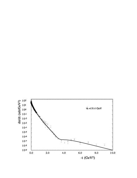
Figure 6: The $d\sigma/dt$ of the $\pi^{-}p$ elastic scattering at $\sqrt{s}=19.4$ GeV ([top] full region of examined $t$ (the corresponding part of the total $\chi^{2}$ given these data is $\chi^{2}/n=442/294=1.5$) and [bottom] small region of $t$ (the corresponding part of the total $\chi^{2}$ given these data is $\chi^{2}/n=166/132=1.26$). [On these figures and others the comparison of the experimental data with theoretical calculations is shown with additional normalization coefficient equal to unity and with only statistical experimental errors] the circles and squares - the experimental data ff1 ; ff2 ; ff3 ; ff4 ; ff5 ).

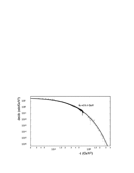
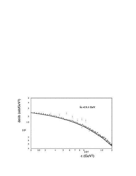
Figure 7: a) The $d\sigma/dt$ of the $\pi^{+}p$ elastic scattering at $\sqrt{s}=19.4$ GeV ([top] full region of examined $t$ (the corresponding part of the total $\chi^{2}$ given these data is $\chi^{2}/n=198/212=0.93$) and [bottom] small region of $t$ (the corresponding part of the total $\chi^{2}$ given these data is $\chi^{2}/n=79.2/79=1.$). the circles and squares - the experimental data ff1 ; ff2 ; ff3 ; ff4 ; ff5 ).

Various Collaborations have determined the PDF sets from inelastic processes only in some region of $x$, which are further approximated to $x=0$ and $x=1$. Also, there is a serious problem in determining the main ingredient of GPDs of a pion - the basic form of parton distribution functions. The predictions based on the perturbative QCD and the calculations using different approaches support the pdf in the form $(1-x)^{2}$ as $x\rightarrow 1$ (see for example Hecht and complicated analysis carried out in Roberts However, the constituent quark model and calculation in the framework of the Nambu-Jona-Lasino model lead to linear behavior $(1-x)_{x\rightarrow 1}$. Several next-to-leading order (NLO) analyses of the Drell-Yan data show that the valence distribution turned out to be rather hard at high momentum fraction x , typically showing only a linear or slightly faster falloff. Correspondingly, there are many different forms of the PDF of a pion. For example, Wat-16 ; Wat-18

$$\nu^{\pi}_{bare}(x,Q^{2}_{0})=A_{0}x^{\alpha}\ (1\ -x)^{\beta}$$

with $\alpha=1.8;\ \beta=1.8$ ;
or (M. Aicher et al. (2010)) Aich10

$$\nu^{\pi}_{bare}(x,Q^{2}_{0})=N_{\nu}x^{\alpha}\ (1\ -x)^{\beta}(1+\gamma x^{2})$$

with $\alpha=1.06;\ \beta=1.75;\ \gamma=1.4$. We examine many of them Mez16 ; Han18 ; Dan19 ; Bour-20 and keep two PDFs leading to approximately the same results and giving the good description of the existence experimental data of pion form factor: one is (L. Chang Mez16 )

$$\nu^{\pi}(x)\ =N\ 3.47\ x^{0.021}\ (1-x)^{2.33};$$ (21)

and R. Sufian Sufian-20

$$\nu^{\pi}(x)=N\frac{x^{-\alpha}\ (1\ -x)^{\beta}(1+\gamma x)}{(B(\alpha+1,\beta+1)-\gamma B(\alpha+2),\beta+1)}$$ (22)

where $B(\alpha,\beta)$ is the incomplete Gamma function. There are two variants: with $\gamma=0$ and with $\gamma=4.28$.

In first variant $\alpha=-0.17$, $\beta=1.24$ and in the second variant $\alpha=-0.22$, $\beta=2.12$. In that work it was noted that both variants give practically the same result.

In our fitting procedure with variation of the slope parameters of the GPDs both variants give close values for the constants of the electromagnetic and gravitomagnetic form factors. In the first case $\Lambda^{2}_{em}=0.49\pm 0.04$ and $\Lambda^{2}_{gr}=1.12\pm 0.15$, and in the second case $\Lambda^{2}_{em}=0.47\pm 0.08$ and $\Lambda^{2}_{gr}=1.07\pm 0.09$,

On the basis of our GPDs with PDFs, we have calculated the pion form factors by numerical integration and then by fitting these integral results by the standard monopole form, which gives the power like scaling Brodsky , and obtained $\Lambda^{2}_{\pi}=0.5$. In Fig.5a, the comparison of our calculation with the existing experimental data of the pion form factor is presented. It is seen that the difference between the calculations of our two chosen PDFs is small, both variants give the $\chi^{2}$ values that are the same within the estimated uncertainty.

The matter form factor $A_{Gr}^{\pi}(t)$ is calculated as the second Mellin moment

$$A_{Gr}^{\pi}(t)=\int^{1}_{0}x\ dx\ q_{\pi}(x)e^{2\alpha_{\pi}f(x)/t}$$ (23)

and is fitted by the simple dipole form $A(t)=\Lambda^{4}/(\Lambda^{2}-t)^{2}$. These form factors will be used in our model of the $\pi^{+}p$ and $\pi^{-}p$ elastic scattering. In Fig.5b, our calculations of the second momentum of GPDs of a pion are shown. Again, we see that the impact of different PDFs is tangible only at large momentum transfer.

VI Hadron form factors and elastic pion-nucleon scattering

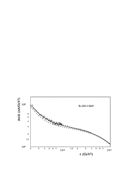
Figure 8: The differential cross sections of the $\pi^{-}p$ elastic cross sections at $\sqrt{s}=25.4$ GeV (the dashed line is the model calculations for the $\pi^{+}p$ elastic cross sections at this energy, points -the data 25p4 ) (the corresponding part of the total $\chi^{2}$ given these data is $\chi^{2}/n=69/57=1.2$).

Let us determine the Born terms of the elastic pion-nucleon scattering amplitude in the same form as we determined the elastic nucleon-nucleon scattering amplitudes. Using both the (electromagnetic and gravitomagnetic) form factors of a pion and a nucleon, we obtain

$$F_{mh}^{Born}(s,t)= h_{1}\ F_{1}(t)\ F_{\pi}(t)\ F_{a}(s,t)$$

$$+h_{2}\ A_{N}(t)\ A^{\pi}_{Gr}(t)\ F_{b}(s,t)\$$

$$\pm R_{c}(s,t),$$

where $F_{\pi}(t)$ is the electromagnetic pion form factor, which represents the charge distribution in the pion and $A^{\pi}_{Gr}(t)$ is the gravitation form factor which represents the matter distribution in the pion, and $F_{a}(s,t)$ and $F_{b}(s,t)$ have the standard Regge form:

$$F_{a}(s,t)=\hat{s}^{\epsilon}(1+(1-k_{2}/(k_{1}\sqrt{\hat{s}}))k_{1}/\sqrt{\hat{s}})e^{B(\hat{s})\ t};$$ (25)

$$F_{b}(s,t)=\hat{s}^{\epsilon}(1+(1+k_{2}/\sqrt{\hat{s}})/\sqrt{\hat{s}})e^{B(\hat{s})/4\ t},$$ (26)

with $\hat{s}=s\ e^{-i\pi/2}/s_{0};\ \ s_{0}=1\ {\rm GeV^{2}}$, and at $t=0$ the intercept $1+\epsilon=1.11$ was chosen the same as for nucleon-nucleon elastic scattering. Hence, at the asymptotic energy we have the universality of the energy behavior of the elastic hadron scattering amplitudes.

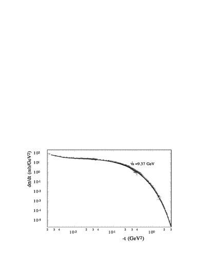
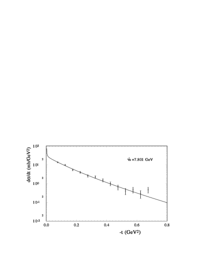
Figure 9: The differential cross sections of the elastic scattering of the $\pi^{-}p$ elastic cross sections at $\sqrt{s}=9.73$ GeV (the line is the model calculations, the squares and circles are the experimental data derev74 ; apokin75 ; ayres76 ; asad84 ) (the corresponding part of the total $\chi^{2}$ given these data is $\chi^{2}/n=213/191=1.1$) and b)[bottom] the $\pi^{+}p$ elastic cross sections at $\sqrt{s}=7.807$ GeV with experimental data azinenko80 (the corresponding part of the total $\chi^{2}$ given these data is $\chi^{2}/n=8/13=0.6$).

The slope of the scattering amplitude has the standard logarithmic dependence on the energy $B(s)=\alpha^{\prime}\ ln(\hat{s})$ with $\alpha^{\prime}=0.24$ GeV^-2 (the same value as for nucleon-nucleon elastic scattering). Examining the pion-nucleon elastic scattering at low energies, we take into account the contributions of the non-leading cross-odd Reggions using the form factors of the pion and nucleon:

$$R_{c}^{Born}(s,t)=h_{c}G_{\pi}(t)G_{N}(t)\frac{i(\pi/2\pm 1)}{\sqrt{\hat{s}}}e^{b_{R}tLn(\hat{s})}.$$ (27)

with the standard Reggion slope $b_{R}=0.9$ GeV^-2.

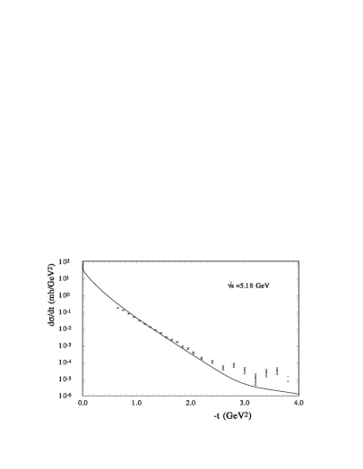
Figure 10: The differential cross sections of the elastic scattering of the $\pi^{+}p$ elastic cross sections at $\sqrt{s}=5.18$ GeV (the line is the model predictions, the points are the experimental data rub73 ).

As a result, only $5$ constants of interaction are included in the fitting procedure. The energy dependence, the momentum transfer dependence and the real part of the scattering amplitude are determined by the complex $\hat{s}$ and intercept. Their values do not change in the fitting procedure. The final elastic hadron scattering amplitude is obtained after unitarization of the Born term. So, at first, we have to calculate the eikonal phase

$$\chi(s,b)\ =-\frac{1}{2\pi}\ \int\ d^{2}q\ e^{i\vec{b}\cdot\vec{q}}\ F^{\rm Born}_{h}(s,q^{2})$$ (28)

and then obtain the final hadron scattering amplitude.

$$F_{h}(s,t)=is\ \int\ b\ J_{0}(bq)\ \Gamma(s,b)\ db\,;$$ (29)

$${\rm with}\ \ \ \ \Gamma(s,b)=1-\exp[\chi(s,b)].$$ (30)

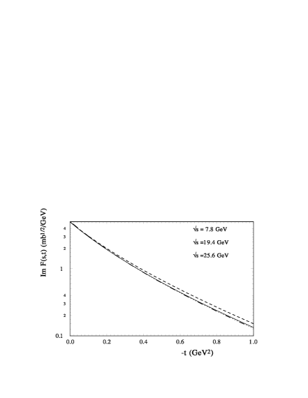
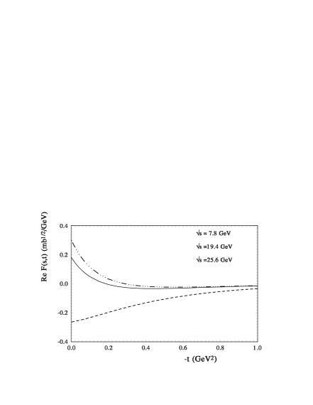
Figure 11: a) [top] The energy and momentum transfer dependence of the imaginary part of the elastic scattering amplitude of $\pi^{-}p$ and
                                    b) [bottom] the real part of the elastic scattering amplitude $\pi^{-}p$ (the dashed, solid and dotted-dashed lines correspond to the $\sqrt{s}=25.3,19.4\ {\rm and}\ 7.8\$ GeV ).

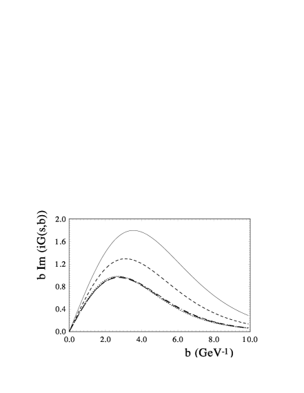
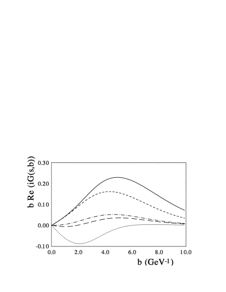
Figure 12: The scattering amplitude of $\pi^{-}p$ elastic scattering in the impact parameter representation - $i\ b\Gamma(s,b)$ a) [top] - the imaginary part and b) [bottom] the real part (the points, long-dashed, dotted-dashed, dashed and solid lines correspond to the $\sqrt{s}=7.8,19.4,25.4,300\ {\rm and}\ 3000\$ GeV ).

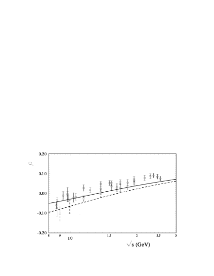
Figure 13: The value $\rho(s,t=0)$ - the ratio of the real to imaginary parts of $\pi^{\pm}p$ elastic scattering amplitude (curves - our model predictions, circles, squares, triangles up and triangles down - Rub19am ; Adam19 ; Schiz19 ; Aker19 ; Cul19 ; Rub19 ; Bri19 ).

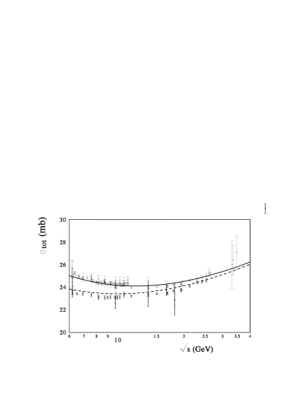
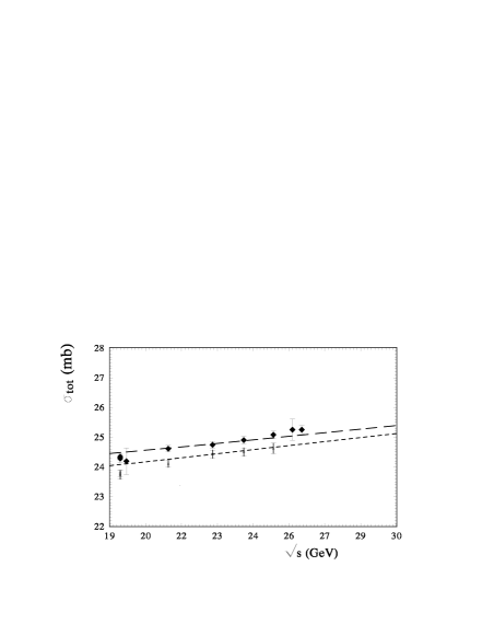
Figure 14: The total cross sections of $\pi^{\pm}p$ elastic scattering a) at low [top], b) at separate energies [middle] and c) high energies [bottom] (curves - our model predictions, circles, squares, triangles up and triangles down - expdata ).

We take into account the experimental data on the $\pi^{+}p$ and $\pi^{-}p$ elastic scattering from $\sqrt{s}=7.807$ GeV up to the maximum measured at $\sqrt{s}=25.46$ GeV. The total number of the experimental data $N_{exp.}=2009$. As in the case of the nucleon scattering, we take into account in the fitting procedure the statistical and systematic errors separately. Only the statistical errors are included in the standard fitting procedure and calculations of $\chi^{2}$. The systematic errors are taken into account as some additional normalization of the experimental data of a separate set. The whole Coulomb-hadron interference region, where the experimental errors are remarkably small, was included in our examination of the experimental data in the region of momentum transfer $0.00137\leq|t|\leq 10$ GeV². After the fitting procedure, with the modern version of FUMILY Sitnik we obtained the total $\sum\chi^{2}_{i}=2415$ and $(\sum\chi^{2})/n_{d.o.f.}=1.2$ (remember that we used only statistical errors). The fitting parameters are obtained as :

$$h_{1}=0.93\pm 0.01;\ h_{2}=1.7\pm 0.02;\ k_{1}=6.7\pm 0.15;$$

$$k_{2}=15.7\pm 0.4;\ \ h_{c}=1.4\pm 0.1$$

The model calculations are compared with the elastic $\pi^{-}p$ (Fig.6) and $\pi^{+}p$ (Fig.7) at $\sqrt{s}=19.4$ GeV. At this energy we have the largest number of experimental data in a wide region of momentum transfer. On these figures and others the comparison of the experimental data with theoretical calculations is shown with additional normalization coefficient equal to unity and with only statistical experimental errors. In Fig.8, such comparison is shown for energy $\sqrt{s}=25.4\$ GeV. It is the highest energy at which we have the experimental data on $\pi^{\pm}p$ elastic scattering from the direct $\pi^{\pm}p$ elastic scattering. Obviously, the model gives a good description of the exiting experimental data, especially in the small $t$ region where the Coulomb-hadron interference plays an important role. The dashed line in Fig.8 shows the model calculations at this energy for $\pi^{+}p$ elastic scattering. It can be seen that the largest difference between $\pi^{-}p$ and $\pi^{+}p$ comes from the Coulomb -hadron interference term which has different signs for these reactions. In Fig.9, the comparison of the model calculations with the experimental data is shown at $\sqrt{s}=9.74$ GeV for $\pi^{-}p$ reactions. At last, in Fig.10, the experimental data of $\pi^{+}p$ elastic scattering are compared with the model predictions. The data are measured up to $-t=4\$GeV². For this energy the latter value corresponds to large angles; however, the model describes the data sufficiently well. Note that in the figures the comparison of the model results with experimental data presented with only statistical errors and does not take into account the experimental systematic uncertainty and our additional normalization coefficients.

The behavior of the imaginary and real parts of the elastic scattering amplitudes at different energies is presented in Fig.11. The imaginary parts have a small energy dependence and their momentum transfer dependence is practically the same in this energy interval. We see different situations for the real parts of the elastic scattering amplitudes. A particularly large difference is shown for low energies. It comes from the non-asymptotic terms of the scattering amplitude.

In Fig.12, the elastic scattering amplitude $ib\Gamma(s,b)$ is presented in the impact parameter representation at energies $\sqrt{s}=7.8,\ 19.4,\ 25.6,\ 300.,\ 3000.$ GeV. The imaginary part of the scattering amplitude essentially grows with energy and its maximum moves to the biggest value of the impact parameter. It reflects the growth of the radius of the hadron interaction. Of most interest is the impact parameter dependence of the real part of the scattering amplitude. If at low energy ($\sqrt{s}=7.8$) its maximum practically coincides with the maximum of the imaginary part (approximately at $2.5$ GeV^-1), then at high energies ($\sqrt{s}=25.6$ GeV) the positions of the maximum are different. The maximum of the imaginary part moves approximately at $3.5$ GeV^-1), but the maximum of the real part moves at $5.5$ GeV^-1). Such a large difference probably shows the changes of the hadron potential of the interactions at large distances with growing interaction energy.

The experimental data of $\sigma_{tot}(s)$ - the total cross sections and $\rho(s,t)$ - the ratio of the real to imaginary parts of the elastic scattering amplitude at $t=0$ are not included in the fitting procedure. These data were extracted from the differential cross sections with some simple model representations. Hence, the inclusions of these data in our fitting procedure will be double account. Let us see what gives the model for these values. In Fig. 13, the energy dependence of the $\rho(s,t=0)$ - ratio of the real to imaginary parts of $\pi^{\pm}p$ elastic scattering is shown. It can be see that the model difference between $\rho(s,t=0)_{\pi^{-}p}$ and $\rho(s,t=0)_{\pi^{+}p}$ is not large. The model calculations coincide with the experimental data at low energy but show less difference between the reactions at high energy. Probably, this is due to the possible simplification of accounting for the contribution from the second Regions. However, in general, the model calculations of $\rho(s,t=0)$ show a good energy dependence for both reactions. In Fig.14 a and b, the energy dependence of $\sigma_{tot}$ for these reactions is presented at low energies (Fig.14a) and high energies (Fig.14b). Obviously, the model reproduces sufficiently well the energy dependence of $\sigma_{tot}$ for both reactions. Note that the last four experimental data ($\sqrt{s}=22.5-25.4\$ GeV) for $\sigma_{tot(\pi^{-}p)}$ usually lie above the theoretical curves. This leads to the opinion of the existence of hard pomeron contributions CMS . Our HEGS model with only 5 fitting parameters and without taking into account the data of $\rho(s,t=0)$ and $\sigma_{tot}(s)$ in the fitting procedure shows that the hard pomeron contributions are not necessary (see Table 1). This is consistent with our conclusion that there is no hard pomeron contribution to elastic nucleon-nucleon scattering NP-hP . In Fig.14b, the model calculations of $\sigma_{tot(\pi^{\pm}p)}(s)$ are presented with experimental data at very large energies. The errors and distributions of the data are very large. However, it can be concluded that the model calculations do not contradict the recent experimental data.

Table 1: The comparison of the model predictions of $\sigma_{tot}(s)$ with the experimental data.

$\sqrt{s}$,GeV	$\sigma_{tot}^{th}(s)\pm\delta^{th}(s)$, mb	$\sigma_{tot}^{exp.}(s)$, mb	exper.
26.4	$25.0\pm 0.7$	$25.25\pm 0.09$	CARROLL-79
33.2	$25.5\pm 0.8$	$26.0\pm 2.1$	DERSCH-99
33.4	$25.6\pm 0.8$	$26.4\pm 1.3$	DERSCH-99
34.7	$25.7\pm 0.9$	$27.1\pm 1.5$	DERSCH-99

However, in general, the model calculations of $\rho(s,t=0)$ show a good energy dependence for both reactions. In Fig.14 a and b, the energy dependence of $\sigma_{tot}$ for these reactions is presented at low energies (Fig.14a) and high energies (Fig.14b). Obviously, the model reproduces sufficiently well the energy dependence of $\sigma_{tot}$ for both reactions. Note that the last four experimental data ($\sqrt{s}=22.5-25.4\$ GeV) for $\sigma_{tot(\pi^{-}p)}$ usually lie above the theoretical curves. This leads to the opinion of the existence of hard pomeron contributions CMS . Our HEGS model with only 5 fitting parameters and without taking into account the data of $\rho(s,t=0)$ and $\sigma_{tot}(s)$ in the fitting procedure shows that the hard pomeron contributions are not necessary (see Table 1). This is consistent with our conclusion that there is no hard pomeron contribution to elastic nucleon-nucleon scattering NP-hP . In Fig.14b, the model calculations of $\sigma_{tot(\pi^{\pm}p)}(s)$ are presented with experimental data at very large energies. The errors and distributions of the data are very large. However, it can be concluded that the model calculations do not contradict the recent experimental data.

VII Conclusion

Generalized Parton Distributions reflect the basic properties of the hadron structure and give a bridge between many different reactions. We have examined the new form of the momentum transfer dependence of GPDs of hadrons to obtain different form factors, including Compton form factors, electromagnetic form factors, transition form factor and gravitomagnetic form factors. Our model of GPDs, based on the analysis of practically all existing experimental data on the electromagnetic form factors of the proton and neutron, leads to a good description of the proton and neutron electromagnetic form factors simultaneously. The chosen form of the momentum transfer dependence of GPDs of the pion (the same as t-dependence of nucleon) allows us to describe the electromagnetic form factor of the pion and obtain the pion gravitomagnetic form factor. The obtained parameters of the form factors of the pion and nucleon satisfy the quark count. As a result, the description of different reactions based on the same representation of the hadron structure was obtained. This especially concerns high energy elastic hadron scattering. The meson High Energy Generalized Structure (mHEGS) model, taking into account the electromagnetic and gravitomagnetic form factors of hadrons, describes well the $\pi^{+}p$ and $\pi^{-}p$ elastic scattering in wide energy ($\sqrt{s}>7$ GeV) and momentum transfer regions with a minimum number of fitting parameters, only 5. The investigation of the nucleon structure shows that the density of the matter in hadrons is more concentrated than the charge density. Our calculations show that the ratio of the radii of the electromagnetic density to the gravitomagnetic density is approximately the same for the nucleon and pion. The model opens up a new way to determining the true form of the GPDs and hadrons structure.

Acknowledgments The author would like to thank O.V. Teryaev for fruitful discussions of some questions considered in the paper.

References

- (1) S. Meissner, A. Metz, M. Schlegel, and K. Goeke, JHEP, 08 (2009) 056.
- (2) C. Lorce and B. Pasquini, JHEP, 09 (2013) 138.
- (3) M. Burkardt and B. Pasquini, Europhys. J., A 52, 161 (2016).
- (4) D. Muller, D. Robaschik, B. Geyer, F.M. Dittes and J. Horejsi, Fortsch. Phys. 42, 101 (1994).
- (5) X.D. Ji, Phys. Lett. 78 , (1997) 610; Phys. Rev D 55 7114 (1997).
- (6) Radyushkin, A.V., Phys. Rev. D 56, 5524 (1997).
- (7) G.R. Goldstein, J.O. Hernandez, S. Liuti, Phys.Rev. D84 034007 (2011).
- (8) M.Diehl et al., Eur.Phys. J. C 39 1 (2005).
- (9) S. Sanielevici, P. Valin, Phys. Rev. D, 32, 586 (1985).
- (10) O. Selyugin, O. Teryaev, Phys. Rev. D 79 033003 (2009);
- (11) O.V. Selyugin, Phys. Rev. D 89 093007 (2014) .
- (12) M. Diehl and P. Kroll, Eur.Phys.J. C73 2397 (2013).
- (13) F. Yuan, Phys.Rev. D 69 051501(R) (2004).
- (14) S. Alekhin, J. Blu”mlein, and S. Moch, Phys.Rev. D 86, 054009 (2012).
- (15) O.V. Selyugin, in Proceedings the XVII Workshop ”High Energy Spin Physics - DSPIN-17”; arxiv: hep-ph-1711.08205.
- (16) F.Taghavi-Shahri, H. Khanpour et al., Phys. Rev. Lett. bf 98, 152001 (2007).
- (17) A. Danagoulian, et. al. (Jefferson Lab Hall A Collaboration), Phys.Rev.Lett., 98152001 (2007).
- (18) M. Guidal, M. V. Polyakov, A. V. Radyushkin, M. Vanderhaeghen, Phys.Rev. D 72 054013 (2005).
- (19) F. Hagelstein, arxiv: 1710.00874
- (20) O.V. Selyugin, Eur.Phys.J. C 72, 2073 (2012).
- (21) O.V. Selyugin, Phys. Rev. D 91 113003 (2015) .
- (22) O. V. Selyugin, Nucl.Phys. A 903, 54 (2013).
- (23) O. V. Selyugin and J.-R. Cudell, AIP Conf. Proc. 1819, 641 040017 (2017).
- (24) O.V. Selyugin, Mod. Phys. Lett. A09 1207 (1994).
- (25) O. V. Selyugin, Phys. Rev. D 60 074028 (1999).
- (26) O. V. Selyugin, Phys.Lett. B 797 134 (2019).
- (27) O. V. Selyugin, Mod. Phys. Lett. A 36, 2150148 (2021).
- (28) O.V. Selyugin, Symmetry, 13, 164 (2021).
- (29) G. Antchev et al. (TOTEM Collaboration), Technical 648 Report No. CERN-EP-2017-335-v3; Eur. Phys. J. C 79, 649 785 (2019).
- (30) G. Antchev et al. [TOTEM Collaboration], Eur.Phys.J. C 79, 861 (2019).
- (31) R. Rubinstein, et al., Phys.Rev. D 30, 1413 (1984).
- (32) M. Adamus et al., Phys.Lett. B186 223 (1987)
- (33) A. Schiz, et al., Phys.Rev. D24 26 (1981).
- (34) Akerlof et al., Phys.Rev. D14 2864 (1976).
- (35) R.L. Cool et al., Phys.Rev. D24 2821 (1981).
- (36) D.S. Ayres et al., Phys.Rev. D15 3105 (1976).
- (37) D. Brick et al., Phys.Rev. D25 294 (1982)
- (38) R. Frezzotti, V. Lubicz, and S. Simula (ETM Collaboration), 661 Phys. Rev. D 79, 074506 (2009).
- (39) L. Chang, C. Mezrag, H. Moutarde, C. Roberts, D. Rodriguez-Quintero, P.C. Tandy Phys. Lett. B 737, 23 (2014).
- (40) W. Melnitchouk, Eur.Phys.J. A17, 223 (2003).
- (41) K. Watanabe, H. Ishikawa and M. Nakagawa, hep-ph/0111168.
- (42) X. Ji, J.-P. Ma, F. Yuan,Phys.Lett. 610 065207 (2000).
- (43) C.D. Roberts, D.G. Richards, N. Horn, L. Chang, arhiv: 2102.01765.
- (44) A. Watanabe, T. Sawada, and C. W. Kao, Phys. Rev D 97, 074015 (2018).
- (45) A. Watanabe, T. Sawada, and C. W. Kao, Phys. Rev. D 97, 074015 (2018).
- (46) M. Aicher, A. Schafer, and W. Vogelsang, Phys. Rev. Lett. 105, 252003 (2010).
- (47) L. Chang, C. Mezrag, H. Moutarde, C.D. Roberts, J. R.-Q., P.C. Tandy, Phys.lett. B 737, 23 (2014).
- (48) C. Bourrely, F. Buccella, and J.-Ch. Peng, Phys. Lett. B 813, 136021 (2021).
- (49) C. Han, H. Xing, X. Wang, Q. Fu, R. Wang, and X. Chen, Phys. Lett. B 800, 135066 (2020).
- (50) M. Ding, K. Raya, D. Binosi, L. Chang, C. D. Roberts, S. M. Schmidt, Phys. Rev. D 101, (2020) 054014.
- (51) R. S. Sufian et.al., Phys.Rev. D102 054508 (2020).
- (52) S.J. Brodsky and G.F. de Teramond, Phys.Rev.]bf D 77, 056007 (2008).
- (53) H. Dahiya, A. Mukherjee, S. Ray, [hep-ph]/0705.3580.
- (54) S.R. Amendolina, et al., Nucl.Phys. B277 168 (1986).
- (55) C.J. Bebek, et al., Phys..Rev. D 17 1693 (1978).
- (56) G.M. Huber, et al., Phys.Rev. C78 045203 (2008).
- (57) H. Ackermann, et al., Nucl.Phys. B137 294 (1978).
- (58) T. Horn, et al., Phys.Rev.Lett. 97 192001 (2006).
- (59) V. Tadevosyan, et al., Phys.Rev. C75 055205 (2007).
- (60) I.M.Sitnik, Comp.Phys.Comm., 209, 199 (2016).
- (61) J.P. Burq, M. Chemarin, M. Chevallier, A.S. Denisov, Nucl.Phys. B 217 285 (1983) .
- (62) V.D. Apokin, et al., Sov.J.Nucl.Phys. 15 530 (1972).
- (63) C. W. Akerlof et al., Phys.Rev. bf D 14 2864 (1976).
- (64) Z. Asad, et al.,(Annecy(LAPP)-CERN-Bohr Inst-Genoa-Oslo-London. Collaboration), Nucl. Phys. B 255 273 (1984).
- (65) A.A. Derevchekov, et al., Phys.Lett. B48 367 (1974).
- (66) I.V. Azhinenko et al., Sov.J.Nucl.Phys. 31 (1980) 337,; Yad.Fiz. 31 (1980) 648-659. Report number: IFVE-79-126.
- (67) R. Rubinstein, P. Cornillon, G. Grindhammer, J. H. Klems, P. O. Mazur, J. Orear, J. Peoples, and W. Faissler. Phys. Rev. Lett. 30 , 1010, (1973).
- (68) R. Cudell, E. Martynov, O. V. Selyugin, and A. Lengyel, Phys. Lett.B 587, 78 (2004).
- (69) M.R. Whalley, Durham HepData Project, http:// durpdg. dur.ac.uk/hepdata/reac.html.
- (70) S. Carroll et al., Phys.Lett. 80B, 423 (1979).
- (71) U. Dersch, et. al., Nuclear Physics, B 579 277 (2000).