First-order nonlinear eigenvalue problems involving functions of a general oscillatory behavior

Abstract

Eigenvalue problems arise in many areas of physics, from solving a classical electromagnetic problem to calculating the quantum bound states of the hydrogen atom. In textbooks, eigenvalue problems are defined for linear problems, particularly linear differential equations such as time-independent Schrödinger equations. Eigenfunctions of such problems exhibit several standard features independent of the form of the underlying equations. As discussed in Bender et al [J. Phys. A 47, 235204 (2014)], separatrices of nonlinear differential equations share some of these features. In this sense, they can be considered eigenfunctions of nonlinear differential equations, and the quantized initial conditions that give rise to the separatrices can be interpreted as eigenvalues. We introduce a first-order nonlinear eigenvalue problem involving a general class of functions and obtain the large-eigenvalue limit by reducing it to a random walk problem on a half-line. The introduced general class of functions covers many special functions such as the Bessel and Airy functions, which are themselves solutions of second-order differential equations. For instance, in a special case involving the Bessel functions of the first kind, i.e., for $y^{\prime}(x)=J_{\nu}(xy)$, we show that the eigenvalues asymptotically grow as $2^{41/42}n^{1/4}$. We also introduce and discuss nonlinear eigenvalue problems involving the reciprocal gamma and the Riemann zeta functions, which are not solutions to simple differential equations. With the reciprocal gamma function, i.e., for $y^{\prime}(x)=1/\Gamma(-xy)$, we show that the $n$th eigenvalue grows factorially fast as $\sqrt{(1-2n)/\Gamma(r_{2n-1})}$, where $r_{k}$ is the $k$th root of the digamma function.

I Introduction

In the context of stability and instability, the idea of nonlinear eigenvalue problems was proposed first in reference Bender et al. (2014) for the nonlinear first-order differential equation

$$y^{\prime}(x)=\cos(\pi xy),\quad y(0)=E_{n}\,,$$ (1)

where $E_{n}$ are the critical initial conditions that give rise to unstable separatrix solutions. Putting the initial condition at the origin aside and tackling the first-order differential equation by expanding its solutions about infinity as $y\sim c/x+\cdots$ yields an asymptotic expansion that does not have any arbitrary constant, while there must exist exactly one; see references (Bender et al., 2014, eq. 5) and (Bender et al., 2010, eq. 48). It turns out the missing, arbitrary constant lies beyond all orders. A hyperasymptotic analysis (asymptotics beyond all orders) reveals the structure of the expansion as well as the arbitrary constant, and it explains the existence of separatrices Bender et al. (2010, 2014). Reference Bender et al. (2014) investigates the discrete spectrum of critical initial conditions associated with the separatrices, interprets them as the eigenvalues of the problem, and calculates the asymptotic behavior of the eigenvalues as well as the separatrices by reducing the nonlinear problem to a linear random-walk problem.

Various nonlinear equations appear in mathematical physics, and it would be interesting to study them in the context of nonlinear eigenvalue problems. Applications of this idea to the Painlevé equations showed that the eigenvalues of the first, second, and fourth Painlevé equations are asymptotically related to cubic, quartic, and sextic anharmonic quantum oscillators, respectively Bender and Komijani (2015, ). Further investigations led to the introduction of a vast class of generalized Painlevé equations Bender et al. (2019). In all cases, the nonlinear problems are reduced to linear ones at the large-eigenvalue limit. In this paper, we extend the program and investigate the first-order differential equation

$$y^{\prime}(x)=F(xy),\quad y(0)=E,$$ (2)

and we obtain the large order behavior of the critical initial values, i.e., eigenvalues, for a general class of generating functions $F$ as well as an isolated example as described below. In the most general case, our solution involves reducing the nonlinear problem to a random walk problem in one dimension.

Reference Bender et al. (2019) discusses the similarities between separatrices of a nonlinear differential equation such as equation (1) and eigenfunctions of linear time-independent Schrödinger equations, and it clarifies the use of terminology eigenfunctions and eigenvalues for nonlinear problems. In particular, reference Bender et al. (2019) explains that eigenvalue problems are inherently unstable because an infinitesimal change in the problem’s parameters violates the boundary conditions. For linear problems, one can explain this instability using the Stokes phenomenon and the Stokes multipliers. (See reference Bender and Orszag (1978) for a pedagogical description of the Stokes phenomenon.) For instance, consider the quantum harmonic oscillator

$$-\psi^{\prime\prime}(x)+\frac{1}{4}x^{2}\psi(x)=\left(\nu+\frac{1}{2}\right)\psi(x)$$ (3)

with the boundary conditions $\psi(\pm\infty)=0$. This is the Weber equation, also known as the parabolic cylinder equation. This equation has a solution in the complex plane denoted by $D_{\nu}(z)$ that is subdominant—vanishes exponentially fast—as $z$ tends to infinity and $|\text{arg}z|<\pi/4$. This special solution satisfies the vanishing boundary condition at $+\infty$, but not necessarily the one at $-\infty$. To find solutions that vanish at both limits, one can exploit the functional relation

$$D_{\nu}(z) =s(\nu)D_{-\nu-1}(-iz)+e^{i\nu\pi}D_{\nu}(-z)\,,$$ (4a)

$$s(\nu) =\frac{\sqrt{2\pi}}{\Gamma(-\nu)}e^{i(\nu+1)\pi/2}\,,$$ (4b)

which relates subdominant solutions of the Weber equation at different regions; see references Bender and Orszag (1978); Kawai and Takei (2005) for more discussions. The coefficient $s(\nu)$ in the above relation is called the Stokes multiplier. Taking the boundary conditions into account, one can argue that the eigenvalues of equation (3) are nothing but the roots of the Stokes multiplier $s(\nu)$, which are non-negative integers, i.e., $\nu\in[0,1,2,\cdots]$. For any other values, even infinitesimally different from a root, solutions of equation (3) cannot satisfy the boundary conditions. This feature is common between the eigenvalues of linear equations such as equation (3) and the nonlinear ones such as equation (1).

By converting equation (3) to a Riccati equation, reference hai Wang introduces an exactly solvable nonlinear eigenvalue problem. That study is important because it presents a unique relationship between a class of nonlinear eigenvalue problems and corresponding linear ones, and it provides another justification for using terminology eigenfunctions and eigenvalues for nonlinear problems. It is noteworthy that converting a Schrödinger equation to a Riccati equation lies at the heart of the WKB method. As we discuss briefly below, in the context of the WKB method, one can interpret a linear eigenvalue problem associated with a second-order Schrödinger-type equation as a special case of a first-order nonlinear eigenvalue problem.

It is evident from the above discussion that the eigenvalues of equation (3) grow algebraically. This behavior is indeed another common feature between many linear and nonlinear eigenvalue problems. For instance, the large eigenvalues of the Schrödinger equation with the class of $\mathcal{PT}$-symmetric Hamiltonians $H=\hat{p}^{2}+g\hat{x}^{2}(i\hat{x})^{\epsilon}$ ($\epsilon>0$) grow as $n^{\gamma}$ with $\gamma=(2\epsilon+4)/(\epsilon+4)$, where $\gamma$ varies between 1 and 2 depending on the value of $\epsilon$. (This result is obtained by using the complex WKB techniques discussed in reference Bender and Boettcher (1998).) Analogously, section II presents a class of nonlinear problems with algebraic growth of eigenvalues as $n^{\gamma}$, where $\gamma$ varies between 0 and infinity.

As an example of algebraic growth of eigenvalues, reference Bender et al. (2014) shows that the eigenvalues $E_{n}$ of the nonlinear equation (1) grow as

$$E_{n}\sim 2^{5/6}n^{1/2}\quad(n\to\infty).$$ (5)

An alternative proof of this asymptotic behavior is given in reference Kerr (2014), and an attempt toward exact WKB analysis of the problem is presented in reference Shigaki (2019). In a similar study, reference Bender et al. (2019) investigates a special case of equation (2) with the generating function $F$ set to the Bessel function of the first kind and order 0 and finds numerically that

$$E_{n}\sim An^{1/4}\quad(n\to\infty),$$ (6)

with $A\approx\frac{35}{18}$. In this paper, we derive this relation analytically and obtain $A=2^{41/42}$. Moreover, we show this asymptotic behavior is valid for all Bessel functions of the first kind and order $\nu\geq 0$. The proof that we provide here is a generalization of the method developed in reference Bender et al. (2014) to tackle equation (1), and it is applicable for a general class of functions $F$ that asymptotically oscillate as

$$F(x)\sim ax^{\alpha}\cos\left(bx^{\beta}+\varphi\right)$$ (7)

as the argument of the function approaches infinity. This is indeed the asymptotic behavior of solutions of ordinary differential equations such as the Bessel and Airy functions on their Stokes lines. We also extend the study to a couple of functions that are not solutions to ordinary differential equations, such as the reciprocal gamma function, which is proportional to the Stokes multiplier of the parabolic cylinder equation, and the Riemann zeta function.

The rest of the paper is organized as follows. In the next section, we discuss nonlinear eigenvalue problems with a class of generating functions $F$ with asymptotic behavior specified in equation (7), and we calculate the large-eigenvalue limit analytically. Numerical solutions of special cases of $F$, namely the Bessel and Airy functions, are also presented in the next section. In section III, we solve a similar problem involving the reciprocal gamma function. Concluding remarks, including a discussion on the zeta function as a generating function and relation between nonlinear and linear eigenvalue problems in the context of the WKB method, are presented in section IV.

II Models with asymptotically oscillatory functions

II.1 Problem definition

In this section, we take into account a general class of generating functions $F$ that satisfy the asymptotic relation

$$F(x)\sim ax^{\alpha}\cos\left(bx^{\beta}+\varphi\right)$$ (8)

as $x\to\infty$. Many functions, including the Bessel and Airy functions, satisfy this asymptotic form on their Stokes lines:

$$J_{\nu}(x)\sim\sqrt{\frac{2}{\pi x}}\cos\left(x-\frac{2\nu+1}{4}\pi\right)$$ (9)

as $x\to\infty$ and

$$\text{Ai}(x)\sim\frac{1}{\sqrt{\pi}(-x)^{1/4}}\cos\left(\frac{2}{3}(-x)^{3/2}-\frac{\pi}{4}\right)$$ (10)

as $x\to-\infty$. With $F$ from such a general class of functions, we define the nonlinear eigenvalue problem

$$y^{\prime}(x)=F\left(xy\right),\quad y(0)=E,$$ (11)

and determine the initial conditions that give rise to separatrix solutions as $x\to\infty$.

Before tackling the problem in its general form, we briefly explore a special case of the problem with the Bessel functions from a numerical point of view. Figure 1 illustrates solutions of

$$y^{\prime}(x)=J_{\nu}(xy),\quad x\geq 0,$$ (12)

with $\nu=0$ (left) and $\nu=1$ (right) for twenty initial values $y(0)$. Among the initial values of each panel, five of them are tuned to critical values (eigenvalues) corresponding to the separatrix solutions shown by dashed curves. One can observe that when the initial condition is slightly different from an eigenvalue, the solution veers away from the corresponding separatrix and gets attracted to a nearby stable asymptotic solution. A hyperasymptotic analysis, similar to the one presented for equation (1) in reference Bender et al. (2014), is required to understand this phenomenon. Because the solutions are qualitatively very similar to the solutions of equation (1), we refer the reader to reference Bender et al. (2014) for a detailed explanation of this phenomenon.

Let us briefly review the properties of the $n$th separatrix in the left (right) panel of figure 1. As $x$ increases from 0, $y(x)$ oscillates with exactly $n$ maxima and then decays to 0 monotonically as $x\to\infty$. This behavior resembles a quantum wave function that oscillates in the so-called classically allowed region and decays in the classically forbidden region. Inspired by high-energy semiclassical calculation of eigenfunctions and eigenvalues in quantum mechanics using the WKB method, we introduce a method to study the asymptotic behavior of the separatrices shown in figure 1 and corresponding eigenvalues. The method that we present here is a generalization of the one developed in reference Bender et al. (2014) to tackle equation (1) and is applicable not only for problems involving the Bessel functions but also for the general case defined in equation (11).

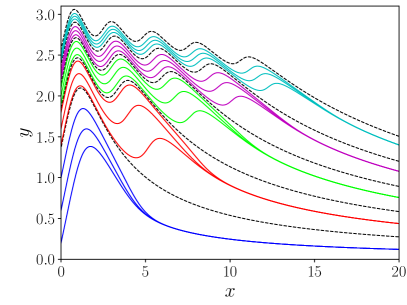
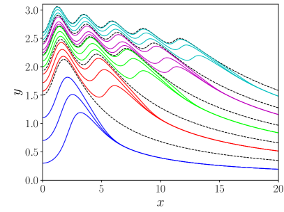
Figure 1: Solutions of equation (12) with $\nu=0$ (left) and $\nu=1$ (right) for twenty initial values. Five of the initial values are tuned to the critical values corresponding to the separatrix solutions shown by dashed curves.

II.2 Asymptotic behavior

The WKB method is a powerful tool to calculate the asymptotic behavior of eigenvalues in quantum mechanics. To this end, the WKB method provides different asymptotic expansions for the wave function, which hold in their respective regions of validity, and then joins them together to obtain a global solution by matching the solutions in neighboring regions. The matching is done in the so-called turning-point regions and puts constraints on possible solutions. In this part, we calculate the asymptotic behavior of eigenvalues in equation (11) following the same strategy of the WKB method. We also employ the quantum-mechanics terminology of classically allowed and forbidden regions as well as turning points.

We assume $a$ and $b$ in equation (8) are real, positive numbers, and we restrict the domain and range of the solutions to $x\geq 0$ and $y\geq 0$, respectively. Unless otherwise stated, we assume $\beta>0$. Under some general conditions on $F$ at the vicinity of origin, the structure of separatrices is then similar to what we observed in figure 1.

To tackle this problem, we use the change of variables

$$y =\sqrt{a}\left(\frac{\lambda}{b}\right)^{\gamma}z\,,$$ (13a)

$$x =\frac{1}{\sqrt{a}}\left(\frac{\lambda}{b}\right)^{\frac{1}{\beta}-\gamma}t\,,$$ (13b)

with $\gamma=(1+\alpha)/(2\beta)$ so that equation (11) asymptotically reads

$$\frac{dz}{dt}\sim(tz)^{\alpha}\cos\left(\lambda(tz)^{\beta}+\varphi\right),$$ (14)

as $\lambda\to\infty$ for a non-vanishing $tz(t)$. We also use the parametrization $\lambda=((2n-\frac{1}{2})\pi-\varphi)$ such that an integer value $n$ corresponds to the ($2n$)th zero of the cosine function and the $n$th eigenvalue of the problem.

The asymptotic solution is simple in the forbidden region $t>1$:

$$z(t)=\frac{1}{t}\left[1-\frac{1}{\beta\lambda}\arcsin\left(\frac{1}{t^{2}}\right)+\text{O}\left(\frac{1}{\lambda^{2}}\right)\right]$$ (15)

as $\lambda\to\infty$. Note that the change of variables that we used puts the turning point of the problem at $t=1$ and results in a solution that approaches unity as $\lambda$ approaches infinity; i.e., $z(1)=1$ at the infinite-$\lambda$ limit. We use this result as the boundary (matching) condition of the solution at $t<1$.

To obtain the solution in the allowed region $t<1$, we multiply the differential equation (14) by $(z+tz^{\prime})z^{-2\alpha}$, and we write it as

$$\frac{1}{2-2\alpha}\frac{d}{dt}z^{2-2\alpha}(t)+\frac{1}{2}t^{1+2\alpha}\left(1+\cos\left(2\lambda(tz)^{\beta}+2\varphi\right)\right)$$

$$\sim\frac{1}{\lambda}\left(\frac{t}{z}\right)^{\alpha}\frac{(tz)^{1-\beta}}{\beta}\frac{d}{dt}\sin\left(\lambda(tz)^{\beta}+\varphi\right)\quad(\lambda\to\infty)\,.$$ (16)

To obtain this relation, we replaced $[z^{\prime}(t)]^{2}$ by equation (14) and used the double-angle formula for the cosine function. Integrating equation (16) from $t_{0}$ to $t$, we obtain:

$$\frac{z^{2-2\alpha}(t)-z^{2-2\alpha}(t_{0})}{1-\alpha}+\frac{t^{2+2\alpha}-t_{0}^{2+2\alpha}}{2+2\alpha}+\eta(t;t_{0}) =\text{O}(1/\lambda)\quad(\lambda\to\infty)\,,$$ (17)

where

$$\eta(t;t_{0})=\int_{t_{0}}^{t}dss^{1+2\alpha}\cos\left(2\lambda(sz(s))^{\beta}+2\varphi\right).$$ (18)

Note that to obtain the right-hand side of equation (17), one can use integration by parts and show that

$$\int_{t_{0}}^{t}ds\frac{1}{\lambda}\left(\frac{s}{z(s)}\right)^{\alpha}\frac{(sz(s))^{1-\beta}}{\beta}\frac{d}{ds}\sin\left(\lambda(sz(s))^{\beta}+\varphi\right)$$

$$=\frac{1}{\beta\lambda}\times\Biggl{\{}\left.\frac{s^{\alpha+1-\beta}}{(z(s))^{\alpha-1+\beta}}\sin\left(\lambda(sz(s))^{\beta}+\varphi\right)\right|_{t_{0}}^{t}$$

$$\quad\qquad-\int_{t_{0}}^{t}ds\frac{d}{ds}\left(\frac{s^{\alpha+1-\beta}}{(z(s))^{\alpha-1+\beta}}\right)\sin\left(\lambda(sz(s))^{\beta}+\varphi\right)\Biggr{\}},$$ (19)

which remains of order $1/\lambda$ as $\lambda\to\infty$.

Solving equation (17) is not trivial, even in the leading order. The right-hand side of equation (17) vanishes at the infinite limit of $\lambda$. The left-hand side, on the contrary, is not easy because it involves $\eta(t;t_{0})$, which is an integral of a complicated, rapidly varying function. We are facing a multiple-scale problem, and because of its nonlinear nature, we cannot exploit well-known methods like the WKB method to solve the problem. To calculate $\eta(t;t_{0})$, we use a method initially developed in reference Bender et al. (2014) and generalize it to fit the current problem. The starting point is to define an infinite set of moments as

$$A_{n,k}(t;t_{0})\equiv\int_{t_{0}}^{t}ds\,s^{1+2\alpha}\cos\left(n\lambda(sz(s))^{\beta}+n\varphi\right)\left(\frac{s^{1+\alpha}}{z^{1-\alpha}(s)}\right)^{k},$$ (20)

and note that $\eta(t;t_{0})=A_{2,0}(t;t_{0})$. These moments are overwhelmingly complicated, but they satisfy a simple, linear difference equation for large $\lambda$:

$$A_{n,k}(t;t_{0})=-\frac{1}{2}A_{n-1,k+1}(t;t_{0})-\frac{1}{2}A_{n+1,k+1}(t;t_{0})\,.$$ (21)

To obtain this equation, we multiply the integrand of the integral in (20) by

$$\frac{z(s)+sz^{\prime}(s)}{z(s)}-\frac{sz^{\prime}(s)}{z(s)}$$ (22)

and then evaluate the first part of the resulting integral by parts and show that it is negligible as $\lambda\to\infty$ if $t_{0}$ and $t$ are not greater than unity. In the second part of the integral, we replace $z^{\prime}(t)$ by equation (14) and use the trigonometric identity

$$\cos(na)\cos(a)=\frac{1}{2}\cos((n+1)a)+\frac{1}{2}\cos((n-1)a)\,.$$ (23)

Let us use $\eta_{\infty}(t;t_{0})$ to denote the infinite-$\lambda$ limit of $\eta(t;t_{0})$. We now exploit the linear difference equation (21) to calculate $\eta_{\infty}(t;t_{0})$. By repeated use of the difference equation, one can expand $\eta_{\infty}(t;t_{0})$ as the series

$$\eta_{\infty}(t;t_{0})=\sum_{p=0}^{\infty}\alpha_{1,2p+1}A_{1,2p+1}(t),$$ (24)

where the coefficients $\alpha_{n,k}$ are determined by a one-dimensional random-walk process in which random walkers move left or right with equal probability but become static when they reach $n=1$. The coefficients can be found in exact form. We refer the reader to reference Bender et al. (2014) for details, and we reproduce the result here:

$$\alpha_{1,2p+1}=\frac{\Gamma(p+1/2)}{\Gamma(-1/2)(p+1)!}\,.$$ (25)

Plugging the coefficients in equation (24), we obtain a series that remarkably can be summed in closed form:

$$\eta_{\infty}(t;t_{0}) =\lim_{\lambda\to\infty}\sum_{p=0}^{\infty}\frac{\Gamma(p+1/2)}{\Gamma(-1/2)(p+1)!}\int_{t_{0}}^{t}ds\,s^{1+2\alpha}z^{\prime}(s)\left(sz(s)\right)^{-\alpha}\left(\frac{s^{2+2\alpha}}{z^{2-2\alpha}(s)}\right)^{p+1/2}$$

$$=\lim_{\lambda\to\infty}\int_{t_{0}}^{t}dsz^{\prime}(s)z^{1-2\alpha}(s)\left(\sqrt{1-\frac{s^{2+2\alpha}}{z^{2-2\alpha}(s)}}-1\right).$$ (26)

The final result is valid for $t_{0}$ and $t$ not larger than unity. Interestingly, there is no explicit reference to $\lambda$ in this expression, and we can safely pass to the limit as $\lambda\to\infty$. In this limit, the function $z(t)$, which is rapidly oscillatory, approaches the function $z_{\infty}(t)$, which is smooth and not oscillatory. The function $z_{\infty}(t)$ obeys

$$\frac{z_{\infty}^{2-2\alpha}(t)-z_{\infty}^{2-2\alpha}(t_{0})}{1-\alpha}+\frac{t^{2+2\alpha}-t_{0}^{2+2\alpha}}{2+2\alpha}+\eta_{\infty}(t;t_{0})=0\,.$$ (27)

We differentiate the above integral equation with respect to $t$ to obtain an elementary differential equation:

$$z_{\infty}^{\prime}(t)z_{\infty}^{1-2\alpha}(t)\left(\sqrt{1-\frac{t^{2+2\alpha}}{z_{\infty}^{2-2\alpha}(t)}}+1\right)+t^{1+2\alpha}=0.$$ (28)

A change of variables as $z_{\infty}^{1-\alpha}(t)=t^{1+\alpha}u(t)$ can easily solve this problem. The result reads

$$\left(z_{\infty}^{1-\alpha}(t)+\frac{\alpha-1}{2}\sqrt{z_{\infty}^{2-2\alpha}(t)-t^{2+2\alpha}}\right)^{2}\left(z_{\infty}^{1-\alpha}(t)+\sqrt{z_{\infty}^{2-2\alpha}(t)-t^{2+2\alpha}}\right)^{1-\alpha}=1,$$ (29)

where the constant on the right-hand side is obtained by matching the solution at the turning point with equation (15), i.e., by imposing the condition $z_{\infty}(1)=1$. This concludes our derivation of $z_{\infty}(t)$.

We now discuss the behavior of $z_{\infty}(t)$ in the vicinity of the origin. Note that our result for $z_{\infty}(t)$ depends only on $\alpha$, and there are three cases depending on the value of $\alpha$:

• If $\alpha>-1$, the $t^{2+2\alpha}$ terms vanish at $t=0$. Consequently, $z_{\infty}(0)$ remains finite and reads

  $$z_{\infty}(0)=\left(\frac{2^{1+\alpha}}{(1+\alpha)^{2}}\right)^{\frac{1}{(1-\alpha)(3-\alpha)}}.$$ (30)

• If $\alpha<-1$, the $t^{2+2\alpha}$ terms diverges at $t=0$. Therefore, as $t\to 0$, we have

  $$z_{\infty}(t)\sim\left(\frac{(1-\alpha)t^{1+\alpha}}{\sqrt{(1-\alpha)^{2}-4}}\right)^{\frac{1}{1-\alpha}}.$$ (31)

• If $\alpha=-1$, as $t\to 0$, we obtain

  $$z_{\infty}(t)\sim\sqrt[4]{-2\ln t}\,.$$ (32)

We conclude that it is only for $\alpha>-1$ that one can define eigenvalues at $t=0$. Using equation (13), we find the asymptotic behavior of the eigenvalues (for $\alpha>-1$):

$$E_{n}\sim An^{\gamma}\quad(n\to\infty),$$ (33)

where $\gamma=(1+\alpha)/(2\beta)$ and

$$A=\sqrt{a}\left(\frac{2\pi}{b}\right)^{\gamma}\left(\frac{2^{1+\alpha}}{(1+\alpha)^{2}}\right)^{\frac{1}{(1-\alpha)(3-\alpha)}}.$$ (34)

This concludes the principal asymptotic analysis of the eigenvalues of equation (11).

II.3 Special cases: Bessel and Airy functions

In the previous part, we calculated the asymptotic behavior of the eigenvalues and eigenfunctions for problems involving functions of general oscillatory behavior. The derived results, namely equations (29), (33), and (34), are valid for all $\beta>0$ and $1+\alpha>0$. The problems specified in equations (1) and (12), with the cosine and Bessel functions, respectively, are special cases of the problem we solved.

Let us now explore equation (12) in the light of the derived results. Performing the change of variables (13), equation (12) reads

$$\frac{dz}{dt}=\sqrt{\frac{\pi\lambda}{2}}J_{\nu}\left(\lambda tz(t)\right).$$ (35)

Then, in the limit of large eigenvalues, $z(t)$ approaches $z_{\infty}(t)$, which is $1/t$ for $t\geq 1$ and

$$\left(4\sqrt{z_{\infty}^{3}(t)}-3\sqrt{z_{\infty}^{3}(t)-t}\right)^{4}\left(\sqrt{z_{\infty}^{3}(t)}+\sqrt{z_{\infty}^{3}(t)-t}\right)^{3} =2^{8}$$ (36)

for $t<1$, and the eigenvalues grow as

$$E_{n} \sim 2^{41/42}n^{1/4}\quad(n\to\infty)\,.$$ (37)

This asymptotic relations yields the overall constant in equation (6): $A=2^{41/42}$.

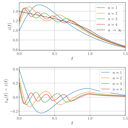
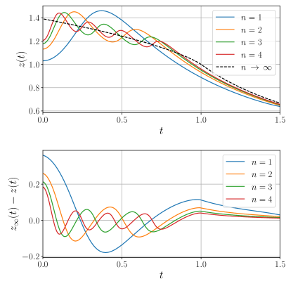
Figure 2: Upper left: the solid curves are the first four eigensolution $z(t)$ of equation (35) with $\nu=0$ corresponding to the Bessel function of order 0. The dashed curve is the large-$n$ limit curve $z_{\infty}(t)$ given in equation (36). Lower left: differences between the solid curves and the dashed curve. Upper and lower right: similar to the upper and lower left panels, respectively, but for the Bessel function of order 1.

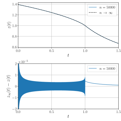
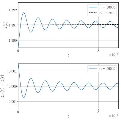
Figure 3: Upper left: the solid line is the $n=50000$ eigensolution to equation (35) with $\nu=0$, and the dashed curve is the large-$n$ limit curve $z_{\infty}(t)$ given in equation (36). Lower left: difference between the solid and dashed curves of the upper left panel. The difference is highly oscillatory and the bulk of the oscillations is of the order $10^{-5}$. Upper and lower right: similar to the upper and lower left panels, respectively, but zoomed in to a region with $t$ of size $1/n$ or smaller.

We now numerically compare the eigensolutions of equation (35) and the large-$\lambda$ limit function $z_{\infty}(t)$. Figure 2 illustrates the first four eigensolutions of $z(t)$ to equation (35) with $\nu=0$ (upper left) and $\nu=1$ (upper right). These eigensolutions have one, two, three, and four maxima, respectively. They oscillate about the large-$\lambda$ limit curve $z_{\infty}(t)$ shown by a dashed curve, and as $n$ increases, the amplitude of oscillations decreases. The lower panels in figure 2 show the difference between the large-$\lambda$ limit curve and the eigensolutions plotted on the upper panels.

Figure 3 shows the $n=50000$ eigensolution to equation (35) with $\nu=0$. The difference between this eigensolution and the large-$\lambda$ limit curve $z_{\infty}(t)$ is not visible in the upper left panel because the amplitude of oscillations is tiny. The lower-left panel shows that the envelope modulating the rapidly oscillating part is of order $1/n$, namely $10^{-5}$. The envelope slowly increases to order $1/\sqrt{n}$, namely $10^{-3}$, as $t$ approaches zero; zoomed in the right panels of figure 3. (We discuss below the size of the envelope analytically.) The $1/\sqrt{n}$ scaling of the envelope at the vicinity of the origin indicates that the next-to-leading order corrections to the eigenvalues $E_{n}$ are of size $1/\sqrt{n}$. Therefore, one needs to go to very high values of $n$ to extract the overall coefficient of the asymptotic behavior of eigenvalues, i.e., to obtain $A$ in equation (6). Moreover, the Richardson extrapolation cannot work well to study the eigenvalues because the central assumption in the Richardson extrapolation is that the corrections to the leading term are of order $1/n$.

Another interesting case involves the Airy function on its Stokes line:

$$y^{\prime}(x)=\text{Ai}(-xy),\quad x\geq 0,$$ (38)

with initial condition $y(0)=E$. Note that the Airy function can be written in terms of the modified Bessel function

$$\text{Ai}(x)=\frac{1}{\pi}\sqrt{\frac{x}{3}}K_{1/3}\left(\frac{2}{3}x^{3/2}\right),$$ (39)

and it obeys the asymptotic relations in equation (10) as $x\to-\infty$. From equation (33), it is evident that the eigenvalues of this problem behave asymptotically as $Bn^{1/4}$, similar to the Bessel function case but with a different multiplicative constant. Figure 4 illustrates the first four and the $n=50000$ (scaled) eigensolutions for the Airy function.

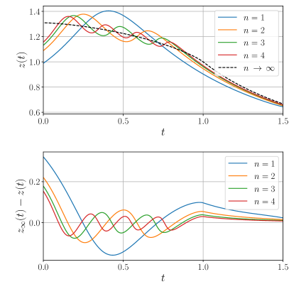
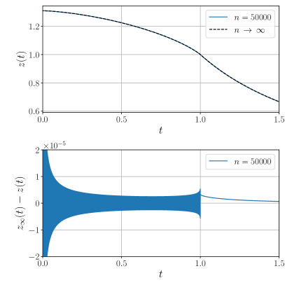
Figure 4: Left and right panels: similar to the left panels of figures 2 and 3, respectively, but for the Airy function.

II.4 Further remarks

We end the discussion of this section with a few remarks.

The numerical solutions illustrated in figures 1, 2, and the left panels of 4 are calculated using the odeint function from the integrate package in scipy, and the ones in figure 3 and the right panels of figure 4 are calculated using an adaptive RK4 method. For precise determination of the separatrix curves, which are unstable and sensitive to numerical round-off errors for increasing $t$, we calculate them backward from large values of $t$ down to the origin. (Note that instability depends on the direction of integration.)

The asymptotic results presented in this section are obtained in the large-eigenvalue limit of the problem, ignoring all terms that vanish in this limit. To calculate the envelope modulating the rapidly oscillating part in the lower panels of figures 3 and 4, one needs to include next-to-leading order terms. Without discussing it in detail, we point out that the envelope can be derived from equation (19):

$$z_{\text{env}}(t)\sim\frac{1}{\beta\lambda}t^{1+\alpha-\beta}z_{\infty}^{\alpha-\beta}(t)$$ (40)

as $t\to 0$. This relation indicates that the difference $z(0)-z_{\infty}(0)$ vanishes like $\lambda^{-2\gamma}$ when $t$ is of order $\lambda^{-1/\beta}$. One then concludes that, for both the Bessel and Airy functions, the envelopes grow like $1/\sqrt{n}$ when $t$ is of order $1/\lambda$. This conclusion agrees with the numerical solutions shown in figures 3 and 4.

So far, we assumed $\beta>0$, but the general results given in equations (33) and (34) are valid for $\beta<0$ too. However, note that the structure of eigensolutions for $\beta<0$ are different from those of the $\beta>0$ cases. For instance, the number of maxima of the eigensolutions is not finite when $\beta<0$ because equation (8) highly oscillates as $x$ approaches zero.

Finally, we point out that $z_{\infty}(t)$ in equation (29) approaches unity as $\alpha$ approaches infinity. As discussed in the next section, this limit is identical to the asymptotic limit of a nonlinear eigenvalue problem involving the reciprocal gamma function.

III A Model with the reciprocal gamma function

In this section, we employ the reciprocal gamma function to define a nonlinear eigenvalue problem:

$$y^{\prime}(x)=\frac{1}{\Gamma(-xy)},\quad x\geq 0,$$ (41)

with initial condition $y(0)=E$. We show that the eigenvalues of this problem behave as

$$E_{n}\sim\sqrt{-\frac{2n-1}{\Gamma(r_{2n-1})}}\quad(n\to\infty),$$ (42)

where $r_{2n-1}$ is the $(2n-1)$th root of the digamma function,

$$r_{\lambda}\approx-\lambda+\frac{1}{\pi}\arctan\left(\frac{\pi}{\log(\lambda+1/8)}\right)\,.$$ (43)

Figure 5 illustrates solutions of equation (41) for several initial values $y(0)$, including the first three eigenvalues. Like the previous examples, $y(x)$ oscillates in an allowed region as $x$ increases from 0 and smoothly decreases in a forbidden region. At large $x$, $y(x)$ asymptotically behaves as $c/x$, where $c=2n-1$ for the $n$th separatrix solution. This behavior can be verified using the identity

$$\frac{1}{\Gamma(-xy)}=-\frac{1}{\pi}\sin(\pi xy)\Gamma(1+xy)\,.$$ (44)

The eigenvalues corresponding to the separatrices grow factorially, as indicated by figure 5. For instance, the tenth and twentieth eigenvalues are $5.50\times 10^{8}$ and $2.86\times 10^{23}$, respectively. They can be compared to $4.98\times 10^{8}$ and $2.68\times 10^{23}$ obtained from equation (42). Because of the factorial growth, double-precision arithmetic cannot handle large eigenvalues.

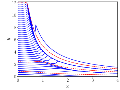
Figure 5: Numerical solutions of equation (41) for several initial values $y(0)$. The red dashed curves are the first three eigensolutions.

To obtain the large-eigenvalue limit, we employ a change of variables as

$$x =\sqrt{\lambda/\xi(\lambda)}\,t\,,$$ (45a)

$$y =\sqrt{\lambda\,\xi(\lambda)}\,z\,,$$ (45b)

where $\lambda=2n-1$ and $\xi(\lambda)$ is a function of $\lambda$ that will be fixed shortly. With this change of variables, equation (41) reads

$$\xi(\lambda)\,\frac{dz}{dt}=\frac{1}{\Gamma\left(-\lambda tz\right)}.$$ (46)

To have a well-defined limit as $\lambda\to\infty$, one can argue that $\xi(\lambda)$ should be

$$\xi(\lambda)=\frac{-1}{{\Gamma(r_{\lambda})}}\xi_{0},$$ (47)

where $r_{\lambda}$ is the $(2n-1)$th root of the digamma function and $\xi_{0}$ is a constant or any function that approaches a constant at the large-$\lambda$ limit. We set $\xi_{0}=1$ and argue below that this choice corresponds to setting the turning point of the problem to $t=1$.

To obtain the asymptotic solution of equation (47) in the forbidden region $t>1$, we start from the following parametrization

$$tz(t)=1-\frac{\epsilon(t)}{\lambda\log(\lambda)}\,.$$ (48)

We then show that as $\lambda\to\infty$, $\epsilon(t)$ satisfies

$$\epsilon(t)e^{-\epsilon(t)}=\frac{\xi_{0}}{t^{2}}e^{-1}\,;$$ (49)

$\epsilon(t)=-W_{0}(-\xi_{0}/(et^{2}))$, where $W_{0}$ is the Lambert $W$ function on its principal branch. The critical point of $W_{0}$ determines the turning point of the problem: $t_{\text{turning}}=\sqrt{\xi_{0}}$. As we wish to put the turning point at unity, we set $\xi_{0}=1$. This choice indicates $z(t)$ approaches unity as $\lambda$ approaches infinity; i.e., $z(1)=1$ at the infinite-$\lambda$ limit. We exploit this result as the boundary (matching) condition for the solution in the allowed region $t<1$, which can be derived easily because one can argue that $\frac{dz}{dt}$ vanished for $t<1$ at the infinite-$\lambda$ limit. Taking the boundary condition at the turning point into account, we conclude that $z(t)$ approaches to

$$z_{\infty}(t)=\begin{cases}1\qquad&t\leq 1\\ 1/t\qquad&t>1\end{cases}$$ (50)

as $\lambda\to\infty$. This result, in turn, yields the asymptotic behavior that we already announced in equation (42).

Figure 6 illustrates the first four eigensolutions of $z(t)$ to equation (46) (left panel) as well as the 80th eigensolution (right panel). The solutions oscillate when $t<1$, but there is a bias compared to the limit curve $z_{\infty}(t)$, unlike other examples discussed above.

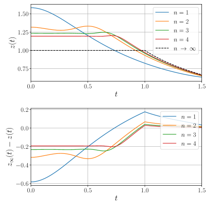
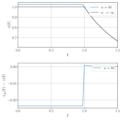
Figure 6: Similar to figure 4 but for the reciprocal gamma function. The right panel shows the scaled eigensolution corresponding to the 80th eigenvalue.

IV Summary and concluding remarks

In this paper, we studied a class of first-order nonlinear eigenvalue problems with generating functions that asymptotically behave as $ax^{\alpha}\cos\left(bx^{\beta}+\varphi\right)$ as $x\to\infty$. This asymptotic behavior is standard among special functions that are solutions of ordinary differential equations on their Stokes lines. Extending the technique developed in reference Bender et al. (2014), we introduced a method to study the asymptotic behavior of large eigenvalues of this nonlinear problem. We can compare our method with the WKB method, which provides a way to calculate this limit for linear eigenvalue problems of Schrödinger-type equations. Consider the linear time-independent Schrödinger equation on the infinite domain $-\infty<x<\infty$

$$-\psi^{\prime\prime}(x)+\eta^{2}\left(V(x)-E\right)\psi(x)=0,\quad\psi(\pm\infty)=0,$$ (51)

where $\eta=1/\hbar$ and $V(x)$ rises at $\pm\infty$. The WKB method constructs solutions of the form

$$\psi(x)=\exp\left(\eta\int^{x}S(t;\eta)dt\right),$$ (52)

where $S(x;\eta)$ satisfies the Riccati equation

$$\eta^{-1}S^{\prime}(x;\eta)=V(x)-E-S^{2}(x;\eta).$$ (53)

One can study this Riccati equation in the context of nonlinear eigenvalue problems. Solving this equation makes it clear that the eigenfunctions of the Schrödinger equation are closely related to the eigenfunctions of the Riccati equation. It is straightforward to obtain the solution of the Riccati equation as an expansion in inverse powers of $\eta$. On the contrary, for the nonlinear eigenvalue problem studied here, it is not easy to accomplish such a mission even in the leading order. Here we could obtain the leading term by reducing the nonlinear problem to a linear random walk problem that can be solved exactly. From a different point of view, the method we developed here can be considered an extension of the WKB method tailored for our nonlinear problem. We believe the exact WKB analysis of this problem can open a new area of research. Reference Shigaki (2019) presents such an attempt toward exact WKB analysis of the nonlinear eigenvalue problem studied in reference Bender et al. (2014), which is only a special case of the problem studied here. On the other hand, the method we developed here might be helpful in extending the WKB method to nonlinear problems.

The Stokes multipliers of linear differential equations provide another class of generating functions for first-order nonlinear eigenvalue problems. In this paper, we investigated the reciprocal gamma function and worked out its large-eigenvalue limit. Another interesting example is the Riemann zeta function $\zeta(z)$. According to the Riemann hypothesis, the nontrivial zeros of $\zeta(z)$ lie on its critical line, and there is a conjecture that the nontrivial zeros are related to eigenvalues of a specific Hamiltonian; see reference Bender et al. (2017) and references there. Instead of the Riemann zeta function itself, it is easier to use the Riemann xi-function $\xi(z)$ to define a nonlinear eigenvalue problem because it is real on the critical line. For simplicity in numerical calculations, we define and use an alternative form of the Riemann xi-function:

$$\bar{\xi}(t)\equiv\frac{1}{\sqrt{2\pi}}\frac{t^{1/4}}{1/4+t^{2}}e^{\frac{\pi}{4}|t|}\xi(1/2+it)$$ (55)

because $\bar{\xi}(t)$, unlike $\xi(1/2+it)$, does not vanish exponentially at large $t$. We define

$$y^{\prime}(x)=\bar{\xi}(xy)$$ (56)

and calculate its eigenvalues and eigensolutions.

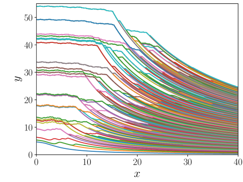
Figure 7: The first 320 eigensolutions of equation (56).

Figure 7 shows the first 320 eigensolutions of equation (56). As the graph indicates, the eigenvalues obtained from this problem inherit the quasi-random nature of the zeros of the zeta function. One can also observe the phenomenon of hyperfine splitting Bender et al. (2019) between different eigenvalues. For instance, the second and third eigenvalues form a set of eigenvalues with hyperfine splitting; see the second (orange) and third (green) curves from below. This problem has fascinating aspects, and we leave it to another paper.

In the above examples, we studied only first-order nonlinear eigenvalue problems. Second-order equations, e.g., the Painlevé equations, provide even a richer area of research. Reference Bender and Komijani (2015) investigates the applications of nonlinear eigenvalue problems to the first and second Painlevé equations and obtains the asymptotic behavior of their eigenvalues by relating these equations to the Schrödinger equation with $\mathcal{PT}$-symmetric Hamiltonian $H=\hat{p}^{2}+g\hat{x}^{2}(i\hat{x})^{\epsilon}$, with $\epsilon=1$ and 2, respectively. References Long et al. ; Long and Zeng obtain the same results at a rigorous level for the first and second Painlevé equations, respectively. Remarkably, the large eigenvalues of the fourth Painlevé are also related to the eigenvalues of the $\mathcal{PT}$-symmetric Hamiltonian with $\epsilon=4$ Bender and Komijani . It would be interesting to extend the study to the third, fifth, and sixth Painlevé equations.

Further investigations in the context of nonlinear eigenvalue problems resulted in introducing a new class of second-order ordinary differential equations called generalized Painlevé equations Bender et al. (2019). Reference Bender et al. (2019) obtains these equations by loosening the so-called Painlevé property such that the movable singularities of solutions can be either poles or fractional powers. Given the fact that the Painlevé equations appear in many areas of mathematical physics—see references Wu et al. (1976); Jimbo and Miwa (1980); Brezin and Kazakov (1990); Douglas and Shenker (1990); Gross and Migdal (1990); Moore (1990a, b); Fokas et al. (1992) for a small sample—although they were initially classified out of theoretical curiosity, one can imagine that the generalized Painlevé equations find their applications in mathematical physics too.