DESY 21-098 June 2021

Renormalization of non-singlet quark operator
matrix elements for off-forward hard scattering
S. Moch${}^{\,a}$ and S. Van Thurenhout${}^{\,a}$
^aII. Institute for Theoretical Physics, Hamburg University
D-22761 Hamburg, Germany
Abstract

We calculate non-singlet quark operator matrix elements of deep-inelastic scattering in the chiral limit including operators with total derivatives. This extends previous calculations with zero-momentum transfer through the operator vertex which provides the well-known anomalous dimensions for the evolution of parton distributions, as well as calculations in off-forward kinematics utilizing conformal symmetry. Non-vanishing momentum-flow through the operator vertex leads to mixing with total derivative operators under renormalization. In the limit of a large number of quark flavors $n_{f}$ and for low moments in full QCD, we determine the anomalous dimension matrix to fifth order in the perturbative expansion in the strong coupling $\alpha_{s}$ in the $\overline{\mbox{MS}}$-scheme. We exploit consistency relations for the anomalous dimension matrix which follow from the renormalization structure of the operators, combined with a direct calculation of the relevant diagrams up to fourth order.

1 Introduction

Within the gauge theory of the strong interaction, quantum chromodynamics (QCD), important nonperturbative information about the hadron structure is obtained from matrix elements of local operators between states with the same or different momenta. Depending on the momentum transfer, such operator matrix elements (OMEs) are used to describe the parton distribution functions (PDFs) in forward kinematics, their off-forward counter-parts, the generalized parton distributions (GPDs) or distribution amplitudes (DAs) for vacuum-to-hadron transitions, such as the pion form factor. Extensive reviews on the description of hadron structure using GPDs and DAs can be found in e.g. [1] and [2]. PDFs or GPDs can be extracted from data for hard inclusive and semi-inclusive reactions with identified particles in the final state, collected for example in deep-inelastic scattering (DIS) in the past at the HERA collider [3, 4] or in the future through the research program at the planned Electron Ion Collider (EIC) [5, 6]. Various DAs can be obtained from data taken in high-intensity, medium energy experiments, for instance at Belle II [7]. All such nonperturbative quantities are also accessible from first principles in QCD simulations of the hadron structure on the lattice, see e.g. [8, 9] and for recent progress [10, 11, 12, 13, 14, 15].

The scale-dependence of such distributions is governed by the renormalization group equations for the corresponding operators and can be computed order by order in the strong coupling $\alpha_{s}$ in perturbative QCD. We focus here on the non-singlet quark OMEs relevant in DIS in the chiral limit and include mixing with operators involving total derivatives. In a given basis of local operators this implies renormalization with a triangular mixing matrix where the diagonal entries are the forward anomalous dimensions, well-known from inclusive DIS, but the off-diagonal elements of the renormalization matrix require a separate calculation.

The anomalous dimensions of non-singlet quark operators as functions of the Mellin moment $N$, which coincides with the Lorentz spin of the operator, are completely known up to three loops [16, 17, 18], and, likewise the corresponding splitting functions in $x$-space. At the four-loop level, low fixed moments [19, 20, 21] and complete results in the limit of a large number $n_{f}$ of quark flavors [22, 23] have been obtained. More recently, fixed moments up to $N=16$ have been computed and used to determine complete analytic results for a general $SU(n_{c})$ gauge theory in the planar limit, i.e. in the limit of a large $n_{c}$ [24]. Partial information consisting of the large $n_{f}$ limit [22] and of low moments [25] is available even at five loops.

In off-forward kinematics, the three-loop evolution kernel for flavor-non-singlet operators is known as well [26]. The computation has exploited conformal symmetry [27] of the QCD Lagrangian which was first utilized in pioneering work for the two-loop radiative corrections [28, 29]. In $d=4-2\epsilon$ dimensions and adopting the modified minimal subtraction ($\overline{\mbox{MS}}$) scheme conformal symmetry in QCD is exact for large $n_{f}$ at the critical coupling. In the physical four-dimensional theory the renormalization group equations then inherit a conformal symmetry so that the generators of the conformal transformations and the evolution kernel commute [30]. Consistency relations following from the conformal algebra allow to restore the $l$-loop triangular mixing matrix for the off-forward anomalous dimensions from the $l$-loop forward anomalous dimensions and an $(l-1)$-loop result for a so-called conformal anomaly [31, 32, 26]. In moment space, the off-forward anomalous dimension depends on the Lorentz spin $N$ as well as on the number $k$ of total derivatives acting on the operator. In momentum space, the corresponding conjugate variables are the momentum fraction $x$ carried by the struck parton and an additional kinematical variable such as the skewedness parameter of the process.

Fixed moments of non-singlet quark OMEs at three-loop order have also been computed in the $\overline{\mbox{MS}}$ renormalization scheme as well as in alternative ones, such as the regularization invariant (RI) scheme, which are suitable for a direct application to available lattice results [33, 34]. The choice for a basis of the renormalized local operators in these works is different from the one in the conformal approach [28], so that a comparison between the fixed moment results of [33, 34] and those of [26, 28, 29] is not immediate, requiring additional computational steps.

In the present article, we review the renormalization of non-singlet quark operators with particular emphasis on possible choices for their bases. In this way, we connect to different results that have appeared as of yet unrelated in the literature. We perform explicit computations of the relevant OMEs up to four loops for non-zero momentum transfer through the operator vertex and derive a number of consistency relations for the respective anomalous dimensions which govern the mixing associated with total derivative operators. This checks and extends previous calculations for the leading-$n_{f}$ terms in the evolution of flavor non-singlet operators in off-forward kinematics up to five loops.

The article is organized as follows: In Sec. 2 we set the stage, review the different basis choices for spin-$N$ local non-singlet quark operators used in the literature and discuss their renormalization together with particular properties of the anomalous dimensions. Details of the computation are given in Sec. 3 and results for the moments of the complete mixing matrix up to five loops for the leading-$n_{f}$ terms are presented in Sec. 4. In Sec. 5, we list some results beyond the leading-${n_{\!f}}$ limit, including the second order mixing matrix in the planar limit and fixed numerical moments in full QCD up to fifth order. The corresponding moments for a general gauge group $SU({n_{c}})$ are deferred to App. A. Conclusions and an outlook are given in Sec. 6.

2 Theoretical framework

We consider the renormalization of spin-$N$ local non-singlet quark operators

$$\mathcal{O}^{NS}_{\mu_{1}\dots\mu_{N}}\,=\,\mathcal{S}\,\overline{\psi}\lambda^{\alpha}\gamma_{\mu_{1}}D_{\mu_{2}}\dots D_{\mu_{N}}\psi\,,$$ (2.1)

where $\psi$ represents the quark field, $D_{\mu}=\partial_{\mu}-ig_{s}A_{\mu}$ the standard QCD covariant derivative, and $\lambda^{\alpha}$ the generators of the flavor group $SU(n_{f})$. Since we focus on the leading-twist contributions, we symmetrize the Lorentz indices and take the traceless part, indicated by ${\mathcal{S}}$. This projects the twist-two contribution, see e.g. [35].

The anomalous dimensions of interest are determined by considering spin-averaged OMEs obtained by inserting the respective operators in two-point functions,

$$\langle\psi(p_{1})|\mathcal{O}_{\mu_{1}\dots\mu_{N}}^{NS}(p_{3})|\overline{\psi}(p_{2})\rangle\,,$$ (2.2)

with quarks and anti-quarks of momenta $p_{1}$ and $p_{2}$ as external fields and all momenta are incoming, $\sum_{i=1}^{3}p_{i}=0$. Choosing $p_{3}=0$ leads to zero momentum-flow through the operator and the OMEs are renormalized with the standard forward anomalous dimensions, see e.g. [24]. For the general case $p_{3}\neq 0$ there is a momentum transfer through the operator vertex, which implies mixing between the operators in Eq. (2.1) and additional total derivative operators.

Next we will introduce three sets of bases commonly used in the literature. One is built from an expansion in Gegenbauer polynomials, which is used in the conformal approach, and the other two are based on counting powers of (total) derivatives.

2.1 The Gegenbauer basis

We start our discussion by introducing the renormalized non-local light-ray operators $[\mathcal{O}]$. These act as generating functions for local operators, see [26], as

$$[\mathcal{O}](x;z_{1},z_{2})\,=\,\sum\limits_{m,k}\frac{z_{1}^{m}z_{2}^{k}}{m!\,k!}\left[\overline{\psi}(x)(\stackrel{{\scriptstyle\leftarrow}}{{D}}\cdot n)^{m}\hbox to0.0pt{\hbox{$\mskip 1.0mu/$}\hss}n(n\cdot\stackrel{{\scriptstyle\rightarrow}}{{D}})^{k}\psi(x)\right]\,.$$ (2.3)

Here, $n$ is an arbitrary light-like vector. For simplicity, the $x$-dependence will be omitted in the following, writing $\mathcal{O}(z_{1},z_{2})\equiv\mathcal{O}(0;z_{1},z_{2})$. The renormalization group equation for these light-ray operators can be written as

$$\Big{(}\mu^{2}\partial_{\mu^{2}}+\beta(a_{s})\partial_{a_{s}}+\mathcal{H}(a_{s})\Big{)}[\mathcal{O}](z_{1},z_{2})=0\,,$$ (2.4)

with $\mu$ the renormalization scale, $a_{s}=\alpha_{s}/(4\pi)$ the strong coupling and $\beta(a_{s})$ the QCD beta-function. The evolution operator $\mathcal{H}(a_{s})$ is an integral operator and acts on the light-cone coordinates of the fields [36]

$$\mathcal{H}(a_{s})[\mathcal{O}](z_{1},z_{2})\,=\,\int_{0}^{1}d\alpha\int_{0}^{1}d\beta\>h(\alpha,\beta)[\mathcal{O}](z_{12}^{\alpha},z_{21}^{\beta})$$ (2.5)

with $z_{12}^{\alpha}\equiv z_{1}(1-\alpha)+z_{2}\alpha$ and the evolution kernel $h(\alpha,\beta)$. The moments of the evolution kernel correspond to the anomalous dimensions of the local operators in Eq. (2.3)

$$\gamma_{N,N}=\int_{0}^{1}d\alpha\int_{0}^{1}d\beta\,(1-\alpha-\beta)^{N-1}h(\alpha,\beta)\,,$$ (2.6)

where $N$ represents the total number of covariant derivatives appearing in the operator, i.e. $N=m+k$ in Eq. (2.3). The forward anomalous dimensions will be represented by $\gamma_{N,N}$, and there is a shift $N\rightarrow N+1$ compared to the literature which is related to the operator definition.

The light-ray operators in Eq. (2.3) admit an expansion in a basis of local operators in terms of Gegenbauer polynomials, see e.g. [37, 29],

$$\mathcal{O}_{N,k}^{\mathcal{G}}=(\partial_{z_{1}}+\partial_{z_{2}})^{k}C^{3/2}_{N}\Big{(}\frac{\partial_{z_{1}}-\partial_{z_{2}}}{\partial_{z_{1}}+\partial_{z_{2}}}\Big{)}\mathcal{O}(z_{1},z_{2})\biggr{|}_{z_{1}=z_{2}=0}\,,$$ (2.7)

where $k\geq N$ is the total number of derivatives and we use the superscript $\mathcal{G}$ to denote the operators in the Gegenbauer basis. For any given $N$, the operator of lowest dimension, $\mathcal{O}_{N,N}^{\mathcal{G}}$, is a conformal operator. The Gegenbauer polynomials can be written in terms of the hypergeometric function ${}_{2}F_{1}$ as [38]

$$C_{N}^{\nu}(z) = \frac{(2\nu)_{N}}{N!}{{}_{2}}F_{1}\Big{(}-N,N+2\nu;\nu+\frac{1}{2};\frac{1}{2}-\frac{z}{2}\Big{)}$$ (2.8)

$$= \frac{\Gamma(\nu+1/2)}{\Gamma(2\nu)}\,\sum\limits_{l=0}^{N}\,(-1)^{l}\frac{\Gamma(2\nu+N+l)}{l!\,(N-l)!\Gamma(\nu+1/2+l)}\,\Big{(}\frac{1}{2}-\frac{z}{2}\Big{)}^{l}\,,$$

where the series representation in terms of the Gamma function will be more convenient for our purposes. The Gegenbauer polynomial with the differential operators then gives

$$(\partial_{z_{1}}+\partial_{z_{2}})^{k}C_{N}^{3/2}\Big{(}\frac{\partial_{z_{1}}-\partial_{z_{2}}}{\partial_{z_{1}}+\partial_{z_{2}}}\Big{)}\,=\,\frac{1}{2N!}\sum\limits_{l=0}^{N}(-1)^{l}\binom{N}{l}\frac{(N+l+2)!}{(l+1)!}\sum\limits_{j=0}^{k-l}\binom{k-l}{j}(\partial_{z_{1}})^{k-l-j}(\partial_{z_{2}})^{l+j}\,,$$

with $k\geq N$. The renormalized operators $[\mathcal{O}_{N,k}^{\mathcal{G}}]$ obey the evolution equation

$$\Big{(}\mu^{2}\partial_{\mu^{2}}+\beta(a_{s})\partial_{a_{s}}\Big{)}[\mathcal{O}_{N,k}^{\mathcal{G}}]\,=\,\sum\limits_{j=0}^{N}\gamma_{N,j}^{\mathcal{G}}[\mathcal{O}_{j,k}^{\mathcal{G}}]\,,$$ (2.10)

where the mixing of the operators is manifest. The anomalous dimension matrix , denoted by $\hat{\gamma}_{N}^{\mathcal{G}}$, is triangular, i.e. its elements $\gamma_{N,j}^{\mathcal{G}}=0$ if $j>N$. It can be computed in QCD perturbation theory and its diagonal elements correspond to the standard forward anomalous dimensions $\gamma_{N,N}$ [24]. Furthermore, the superscript ${\mathcal{G}}$ can be dropped for $\gamma_{N,N}$ since they do not depend on the particular choice for the basis of additional total derivatives. The matrix $\hat{\gamma}_{N}^{\mathcal{G}}$ is currently known up to the three-loop level [26] and we will discuss these results in more detail in Sec. 4.

2.2 The total derivative basis

Another basis for the quark operators, which directly generalizes Eq. (2.1) is

$$\mathcal{O}_{p,q,r}^{\mathcal{D}}\,=\,\mathcal{S}\,\partial^{\mu_{1}}\dots\partial^{\mu_{p}}\,((D^{\nu_{1}}\dots D^{\nu_{q}}\overline{\psi})\,\lambda^{\alpha}\gamma_{\mu}\,(D^{\sigma_{1}}\dots D^{\sigma_{r}}\psi))\,,$$ (2.11)

see e.g. [39, 40] and [41, 35]. Here the superscript $\mathcal{D}$ indicates that the operators are written in the total derivative basis and the indices $p$, $q$ and $r$ count the powers of the respective derivatives. In practical calculations, all Lorentz indices are contracted with a light-like vector $\Delta$, such that the indices $p$, $q$ and $r$ in Eq. (2.11) identify a given operator uniquely. Because of the chiral limit, the partial derivatives act as

$$\mathcal{O}_{p,q,r}^{\mathcal{D}}\,=\,\mathcal{O}_{p-1,q+1,r}^{\mathcal{D}}+\mathcal{O}_{p-1,q,r+1}^{\mathcal{D}}\,.$$ (2.12)

For the bare operators this defines a recursion, which is solved by

$$\mathcal{O}_{p,q,r}^{\mathcal{D}}\,=\,\sum\limits_{i=0}^{p}\,\binom{p}{i}\,\mathcal{O}_{0,p+q-i,r+i}^{\mathcal{D}}\,.$$ (2.13)

Another consequence of the chiral limit is that left and right derivative operators renormalize with the same renormalization constants

$$\mathcal{O}_{p,0,r}^{\mathcal{D}} = \sum\limits_{j=0}^{r}\,Z_{r,r-j}\,[\mathcal{O}_{p+j,0,r-j}^{\mathcal{D}}]\,,$$ (2.14)

$$\mathcal{O}_{p,q,0}^{\mathcal{D}} = \sum\limits_{j=0}^{q}\,Z_{q,q-j}\,[\mathcal{O}_{p+j,q-j,0}^{\mathcal{D}}]\,.$$ (2.15)

The anomalous dimensions $\gamma_{N,k}^{\mathcal{D}}$ governing the scale dependence of these operators are derived from the $Z$-factors by

$$\gamma_{N,k}^{\mathcal{D}}\,=\,-\,\bigg{(}\,\frac{d}{d\ln\mu^{2}}\;Z_{N,j}\bigg{)}\,Z_{j,k}^{\,-1}\,.$$ (2.16)

The mixing matrix is also triangular in the total derivative basis ($\gamma_{N,k}^{\mathcal{D}}=0$ if $k>N$) and, as was the case for the Gegenbauer basis, the diagonal elements are the standard forward anomalous dimensions $\gamma_{N,N}$ [24], where we have also dropped the superscript ${\mathcal{D}}$ due to the basis independence.

It is possible to relate the two operator bases using the light-ray operators in Eq. (2.3) as generating functions. Starting from the bare operators we have

$$\mathcal{O}(z_{1},z_{2})\,=\,\sum\limits_{m,k}\,\frac{z_{1}^{m}z_{2}^{k}}{m!\,k!}\,\mathcal{O}_{0,m,k}^{\mathcal{D}}\,,$$ (2.17)

so that Eqs. (2.7), (2.1) and (2.13) give

$$\mathcal{O}_{N,k}^{\mathcal{G}}\,=\,\frac{1}{2N!}\,\sum\limits_{l=0}^{N}\,(-1)^{l}\binom{N}{l}\,\frac{(N+l+2)!}{(l+1)!}\,\mathcal{O}_{k-l,0,l}^{\mathcal{D}}\,.$$ (2.18)

The evolution equation for the operators $\mathcal{O}_{N,k}^{\mathcal{G}}$ in Eq. (2.10) relates the anomalous dimension matrices in the two bases

$$\sum\limits_{j=0}^{N}\,\gamma_{N,j}^{\mathcal{G}}\,[\mathcal{O}_{j,N}^{\mathcal{G}}]\,=\,\frac{1}{2N!}\,\sum\limits_{l=0}^{N}\,(-1)^{l}\binom{N}{l}\frac{(N+l+2)!}{(l+1)!}\,\sum\limits_{j=0}^{l}\,\gamma_{l,l-j}^{\mathcal{D}}\,[\mathcal{O}_{N-l+j,0,l-j}^{\mathcal{D}}]\,.$$ (2.19)

Using Eq. (2.18) for renormalized operators the left-hand side can be expanded in the operators of the total derivative basis,

$$\sum\limits_{j=0}^{N}\,\gamma_{N,j}^{\mathcal{G}}\,\Bigg{(}\frac{1}{2j!}\sum\limits_{l=0}^{j}\,(-1)^{l}\binom{j}{l}\,\frac{(j+l+2)!}{(l+1)!}\,[\mathcal{O}_{N-l,0,l}^{\mathcal{D}}]\Bigg{)}\,\,$$ (2.20)

$$= \frac{1}{2N!}\,\sum\limits_{j=0}^{N}\,(-1)^{j}\binom{N}{j}\,\frac{(N+j+2)!}{(j+1)!}\,\sum\limits_{l=0}^{j}\gamma_{j,l}^{\mathcal{D}}\,[\mathcal{O}_{N-l,0,l}^{\mathcal{D}}]\,,$$

and upon comparing the coefficients of the operators $[\mathcal{O}_{N-l,0,l}^{\mathcal{D}}]$, we find

$$\sum\limits_{j=0}^{N}\,(-1)^{j}\frac{(j+2)!}{j!}\,\gamma_{N,j}^{\mathcal{G}}\,=\,\frac{1}{N!}\,\sum\limits_{j=0}^{N}\,(-1)^{j}\binom{N}{j}\frac{(N+j+2)!}{(j+1)!}\,\sum\limits_{l=0}^{j}\,\gamma_{j,l}^{\mathcal{D}}\,.$$ (2.21)

To get the expression on the left-hand side, we have evaluated the sum

$$\sum\limits_{l=0}^{j}\,(-1)^{l}\binom{j}{l}\,\frac{(j+l+2)!}{(l+1)!}\,=\,(-1)^{j}(j+2)!\,.$$ (2.22)

2.3 The Geyer basis

The local operators introduced by B. Geyer in [41, 35] are expressed in a basis different from the one in Eq. (2.14), but the quoted anomalous dimensions can be related to $\gamma_{N,k}^{\mathcal{D}}$ in Eq. (2.16). The basis for the local operators used in those references is

$$\mathcal{O}_{N,k}^{\mathcal{B}}\,=\,\overline{\psi}\gamma(\stackrel{{\scriptstyle\rightarrow}}{{D}}+\stackrel{{\scriptstyle\leftarrow}}{{D}})^{N-k}(\stackrel{{\scriptstyle\leftarrow}}{{D}}-\stackrel{{\scriptstyle\rightarrow}}{{D}})^{k}\psi\,.$$ (2.23)

with $N,k$ odd. The superscript $\mathcal{B}$ indicates that the operators are written in the Geyer basis. The contraction with an arbitrary light-like vector is understood, i.e.

$$\gamma\,\equiv\,\Delta^{\mu}\>\gamma_{\mu}\,,\qquad D\,\equiv\,\Delta^{\mu}\>D_{\mu}\,,$$ (2.24)

and $\Delta^{2}=0$.

We now want to relate the operators, and the corresponding anomalous dimensions, in the $\mathcal{B}$-basis to those in the derivative basis. For this we use

$$\mathcal{O}^{\mathcal{D}}_{0,N-k,k}=(-1)^{k}\sum_{j=0}^{k}\binom{k}{j}\mathcal{O}^{\mathcal{D}}_{j,N-j,0},$$ (2.25)

which can be derived in the same way as Eq. (2.13). It is then straightforward to see that, for $k=0$, the operators defined above correspond to total derivatives of the vector current, i.e.

$$\mathcal{O}^{\mathcal{B}}_{N,0}=\mathcal{O}^{\mathcal{D}}_{N,0,0}.$$ (2.26)

For arbitrary $k$-values, we can use the binomial theorem (twice) together with Eq. (2.25). This leads to the following relation between the bare operators

$$\mathcal{O}^{\mathcal{B}}_{N,k}=\sum_{i=0}^{N-k}\sum_{j=0}^{k}(-1)^{i}\binom{N-k}{i}\binom{k}{j}\sum_{l=0}^{i+j}(-1)^{l}\binom{i+j}{l}\mathcal{O}^{\mathcal{D}}_{l,N-l,0}.$$ (2.27)

The corresponding relation for the renormalized operators reads

$$[\mathcal{O}^{\mathcal{B}}_{N,k}]= \sum_{i=0}^{N-k}\sum_{j=0}^{k}(-1)^{i}\binom{N-k}{i}\binom{k}{j}\sum_{l=0}^{i+j}(-1)^{l}\binom{i+j}{l}\sum_{m=0}^{N-l}(-1)^{m}\>\gamma_{N-l,m}^{\mathcal{D}}$$

$$\times\sum_{n=0}^{m}(-1)^{n}\binom{m}{n}[\mathcal{O}^{\mathcal{D}}_{N-m+n,0,m-n}].$$ (2.28)

Like in the Gegenbauer basis, we now focus on the diagonal operators $\mathcal{O}^{\mathcal{B}}_{N,N}$, the evolution equation for which is

$$\mu^{2}\frac{d}{d\mu^{2}}\mathcal{O}_{N,N}^{\mathcal{B}}=\sum_{k=0}^{N}\frac{1-(-1)^{k}}{2}\gamma_{N,k}^{\mathcal{B}}[\mathcal{O}^{\mathcal{B}}_{k,N}]$$ (2.29)

with $N$ odd. Like in the other operator bases, the anomalous dimension matrix $\hat{\gamma}_{N}^{\mathcal{B}}$ is triangular ($\gamma_{N,k}^{\mathcal{B}}=0$ if $k>N$) and in analogy to Eq. (2.21) $\gamma_{N,k}^{\mathcal{B}}$ can be related to the mixing matrices in the Gegenbauer and the total derivative bases. Details will be given below in Sec. 4.1.

2.4 Constraints on the anomalous dimensions

The elements of the mixing matrices for the operators in the total derivative basis are not all independent, but subject to particular constraints, which define useful relationships between them in the chiral limit. Starting from Eq. (2.12) we can derive the following relation by acting $N$ times with a partial derivative on the bare operator $\mathcal{O}_{N,0,0}^{\mathcal{D}}$

$$\mathcal{O}_{0,N,0}^{\mathcal{D}}-(-1)^{N}\sum_{j=0}^{N}(-1)^{j}\binom{N}{j}\mathcal{O}_{j,0,N-j}^{\mathcal{D}}\,=\,0\,.$$ (2.30)

Upon using the renormalization equations (2.14), this leads to a connection between the renormalized operators

$$\sum_{k=0}^{N}\sum_{j=k}^{N}\Bigg{\{}(-1)^{k}\binom{j}{k}Z_{N,j}-(-1)^{j}\binom{N}{j}Z_{j,k}\Bigg{\}}[\mathcal{O}_{N-k,0,k}^{\mathcal{D}}]\,=\,0\,.$$ (2.31)

Now, since the coefficient of $[\mathcal{O}_{N-k,0,k}^{\mathcal{D}}]$ has to vanish for each value of $k$, this becomes a relation between the renormalization constants

$$\forall k:\qquad\sum_{j=k}^{N}\Bigg{\{}(-1)^{k}\binom{j}{k}Z_{N,j}-(-1)^{j}\binom{N}{j}Z_{j,k}\Bigg{\}}\,=\,0\,,$$ (2.32)

which is equivalent to a relation between sums of elements of the mixing matrix $\hat{\gamma}_{N}^{\mathcal{D}}$,

$$\forall k:\qquad\sum_{j=k}^{N}\Bigg{\{}(-1)^{k}\binom{j}{k}\gamma_{N,j}^{\mathcal{D}}-(-1)^{j}\binom{N}{j}\gamma_{j,k}^{\mathcal{D}}\Bigg{\}}\,=\,0\,.$$ (2.33)

This is a general statement, valid to all orders in $a_{s}$. It can be considered as a consequence of parity conservation. If one takes a basis with $\partial_{z_{1}}-\partial_{z_{2}}$ as in Eq. (2.7), i.e., "left minus right (l-r)" derivatives, each such derivative changes parity so that the operators with an even number of "l-r" derivatives do not mix with operators with an odd number of "l-r" derivatives. 

By putting $k=N-1$ we can relate the next-to-diagonal elements of the mixing matrix to the forward anomalous dimensions $\gamma_{N,N}$, cf. Eq. (2.6) ,

$$\gamma_{N,N-1}^{\mathcal{D}}\,=\,\frac{N}{2}\left(\gamma_{N-1,N-1}-\gamma_{N,N}\right)\,,$$ (2.34)

where, as above, the superscript ${\mathcal{D}}$ can be omitted for $\gamma_{N,N}$.

The case $k=0$ in Eq. (2.33) gives

$$\sum_{j=0}^{N}\Bigg{\{}\gamma_{N,j}^{\mathcal{D}}-(-1)^{j}\binom{N}{j}\gamma_{j,0}^{\mathcal{D}}\Bigg{\}}\,=\,0\,,$$ (2.35)

which relates the sum of the elements in the $N$-th row of the mixing matrix to the conjugate $\mathcal{C}\,\gamma_{N,0}^{\mathcal{D}}$ of the last column defined as

$$\mathcal{C}\,\gamma_{N,0}^{\mathcal{D}}\,\equiv\,\sum_{i=0}^{N}(-1)^{i}\binom{N}{i}\,\gamma_{i,0}^{\mathcal{D}}\,,$$ (2.36)

see e.g. [42].

With the help of Eq. (2.35) for the last column of the mixing matrix another relation between the anomalous dimensions in the total derivative basis and the Gegenbauer one can be obtained. Substituting Eq. (2.35) into Eq. (2.21) one finds

$$\sum_{j=0}^{N}(-1)^{j}\frac{(j+2)!}{j!}\gamma_{N,j}^{\mathcal{G}}\,=\,\frac{1}{N!}\sum_{j=0}^{N}(-1)^{j}\binom{N}{j}\frac{(N+j+2)!}{(j+1)!}\sum_{l=0}^{j}(-1)^{l}\binom{j}{l}\gamma_{l,0}^{\mathcal{D}}\,.$$ (2.37)

Considering now arbitrary $k$ in Eq. (2.33) results in

$$\gamma_{N,k}^{\mathcal{D}}\,=\,\binom{N}{k}\sum_{j=0}^{N-k}(-1)^{j}\binom{N-k}{j}\gamma_{j+k,j+k}+\sum_{j=k}^{N}(-1)^{k}\binom{j}{k}\sum_{l=j+1}^{N}(-1)^{l}\binom{N}{l}\gamma_{l,j}^{\mathcal{D}}\,.$$ (2.38)

This is a useful relation for several reasons. Its derivation only relies on the chiral limit, which imposes constraints on the renormalization structure of the operators. It can, therefore, be used as an order-independent consistency check, which any expression for $\gamma_{N,k}^{\mathcal{D}}$ has to obey. Alternatively, Eq. (2.38) provides a path for the construction of the full mixing matrix $\hat{\gamma}_{N}^{\mathcal{D}}$ from the knowledge of the forward anomalous dimensions $\gamma_{N,N}$ and the last column $\gamma_{N,0}^{\mathcal{D}}$ at any order of perturbation theory.

Thus, with partial information being available even to five-loop order, one can construct an ansatz for the off-diagonal elements and use Eq. (2.38) to test its self-consistency. In this case, $\gamma_{N,0}^{\mathcal{D}}$ serves as boundary condition and Eq. (2.34) as a cross-check. This leads to the following 4-step algorithm for the construction of the mixing matrix:

1. Starting from the forward anomalous dimensions $\gamma_{N,N}$ and the bare OMEs in Eq. (2.2), one determines the all-$N$ expressions for the next-to-diagonal $\gamma_{N,N-1}^{\mathcal{D}}$ and the last column entries $\gamma_{N,0}^{\mathcal{D}}$ of the mixing matrix. In the next section, it will be detailed how to relate the last column entries to the calculation of Feynman diagrams.

2. Next, one calculates the sum

   $$\binom{N}{k}\,\sum_{j=0}^{N-k}\,(-1)^{j}\binom{N-k}{j}\,\gamma_{j+k,j+k}\,.$$ (2.39)

   Based on the structure of the result, one can then make an ansatz for the off-diagonal elements.

3. One calculates the double sum

   $$\sum_{j=k}^{N}\,(-1)^{k}\binom{j}{k}\,\sum_{l=j+1}^{N}\,(-1)^{l}\binom{N}{l}\,\gamma_{l,j}^{\mathcal{D}}$$ (2.40)

   with the chosen ansatz and collects everything into Eq. (2.38). This leads to a system of equations in the unknown coefficients of the ansatz. It should be mentioned that Eq. (2.38) by itself is not enough to determine a unique solution for $\gamma_{N,k}^{\mathcal{D}}$. In particular, some structures might be self-conjugate, like e.g.

   $$\sum_{j=k}^{N}\,(-1)^{k}\binom{j}{k}\,\sum_{l=j+1}^{N}\,(-1)^{l}\binom{N}{l}\,\frac{1}{l-j}=-\frac{1}{N-k}.$$ (2.41)

   Uniqueness of the solution is saved however by the fact that there is a boundary condition, namely the expression for $\gamma_{N,k}^{\mathcal{D}}$ has to agree with the previously found expression for $\gamma_{N,0}^{\mathcal{D}}$ from step 1.

4. If the system of equations can be solved consistently, one has determined the final expression for the off-diagonal terms of the mixing matrix $\hat{\gamma}_{N}^{\mathcal{D}}$. If not, the structure of the remaining terms in Eq. (2.38) can be used to adapt the ansatz, leading one back to step 3.

This approach will be applied and described in further detail below.

3 Calculation in Mellin $N$-space

We will describe the computation of Feynman diagrams for the matrix elements of operators in Eq. (2.1) along with the necessary details for the renormalization. The constraints for the anomalous dimensions in Eq. (2.33) and the constructive algorithm to determine the mixing matrix lead to particular types of symbolic sums and techniques for their evaluation will be reviewed as well.

3.1 Calculating Feynman diagrams

We calculate the spin-averaged OMEs defined in Eq. (2.2). To ensure tracelessness and symmetry of the Lorentz indices, the OMEs are contracted with a tensor of light-like $\Delta$,

$$\Delta^{\mu_{1}}\dots\Delta^{\mu_{N}}\,,$$ (3.1)

and $\Delta^{2}=0$. OMEs in off-forward kinematics require momentum-flow through the operator vertex, $p_{3}\neq 0$, see Fig. 1. For simplicity but without loss of generality, one can choose $p_{2}=0$, so that the calculated OMEs are of the form

$$\Delta^{\mu_{1}}\dots\Delta^{\mu_{N}}\,\langle\psi(p_{1})|O_{\mu_{1}\dots\mu_{N}}^{NS}(-p_{1})|\overline{\psi}(0)\rangle\,.$$ (3.2)

With this momentum configuration the OMEs in Eq. (2.2), which are a priori three-point functions reduce effectively to two-point ones, i.e. one is left with massless propagator-type Feynman diagrams. These can be efficiently calculated using computer algebra methods as will be detailed next.

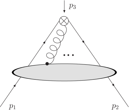
Figure 1: The Green’s function $\langle\psi(p_{1})|O_{\mu_{1}\dots\mu_{N}}^{NS}(p_{3})|\overline{\psi}(p_{2})\rangle$ with momentum $p_{3}=-p_{1}-p_{2}$ flowing through the operator vertex. For simplicity, we set $p_{2}\equiv 0$.

The computations follow a well-established workflow. The Feynman diagrams are generated using Qgraf [43], the output of which is then directed to a Form [44, 45] program to determine the topologies and to compute the color factors of the diagrams, the latter part based on the algorithms presented in [46]. The necessary Feynman rules are given for example in [24]. For computational efficiency, diagrams of the same topology and color factor are grouped together in so-called meta-diagrams, cf. [47] for further details on the use of Form in Feynman diagram calculations. The handling of the meta-diagrams is done with the database program Minos [48]. The actual diagram calculations are then performed using the Forcer program [49], which can efficiently deal with massless propagator-type diagrams in $d=4-2\epsilon$ dimensional regularization [50, 51] up to four loops. In this way we can obtain fixed moments of the OMEs in Eq. (3.2). Finally, the calculations are done using a general covariant gauge. Although the operators considered are gauge invariant, the OMEs will in general depend on the gauge parameter. Using a general covariant gauge, the independence of the anomalous dimensions of the gauge parameter then provides a check on our calculations.

For the renormalization we use the $\overline{\mbox{MS}}$-scheme [52, 53]. In this scheme, the evolution of the strong coupling is governed by

$$\frac{da_{s}}{d\ln\mu^{2}}=\beta(a_{s})=-a_{s}(\epsilon+\beta_{0}a_{s}+\beta_{1}a_{s}^{2}+\beta_{2}a_{s}^{3}+\dots)$$ (3.3)

with $\beta(a_{s})$ the standard QCD beta-function and $\beta_{0}=(11/3){C_{A}}-(2/3){n_{\!f}}$. Writing out Eq. (2.14), the operators are then renormalized as

$$\mathcal{O}_{N+1}=Z_{\psi}\,(Z_{N,N}\mathcal{[}{O}_{N+1}]+Z_{N,N-1}[\partial\mathcal{O}_{N}]+\dots+Z_{N,0}[\partial^{N}\mathcal{O}_{1}])\,,$$ (3.4)

where the quark wave function renormalization factor $Z_{\psi}$ takes care of the self-energy corrections for the off-shell external quarks and we have abbreviated, cf. Eq. (3.1),

$$\Delta^{\mu_{1}}\dots\Delta^{\mu_{N}}\,\mathcal{O}^{NS}_{\mu_{1}\dots\mu_{N}}\,\equiv\,\mathcal{O}_{N}\,.$$ (3.5)

In this notation, $\mathcal{O}_{1}$ simply represents the vector current

$$\mathcal{O}_{1}\,=\,\Delta^{\mu}\,\overline{\psi}\lambda^{\alpha}\gamma_{\mu}\psi.$$ (3.6)

Since this is a conserved quantity, its anomalous dimension vanishes and $Z_{0,0}=1$. For the full set of operators up to spin $(N+1)$, the renormalization takes the form of a matrix equation

$$\begin{pmatrix}\mathcal{O}_{N+1}\\ \partial\mathcal{O}_{N}\\ \vdots\\ \partial^{k}\mathcal{O}_{N+1-k}\\ \vdots\\ \partial^{N}\mathcal{O}_{1}\end{pmatrix}\,=\,Z_{\psi}\begin{pmatrix}Z_{N,N}&Z_{N,N-1}&...&Z_{N,N-k}&...&Z_{N,0}\\ 0&Z_{N-1,N-1}&...&Z_{N-1,N-k}&...&Z_{N-1,0}\\ \vdots&\vdots&...&\vdots&...&\vdots\\ 0&0&...&Z_{N-k,N-k}&...&Z_{N-k,0}\\ \vdots&\vdots&...&\vdots&...&\vdots\\ 0&0&...&0&...&1\end{pmatrix}\begin{pmatrix}[\mathcal{O}_{N+1}]\\ [\partial\mathcal{O}_{N}]\\ \vdots\\ [\partial^{k}\mathcal{O}_{N+1-k}]\\ \vdots\\ [\partial^{N}\mathcal{O}_{1}]\end{pmatrix}\,.$$ (3.7)

Note that the bottom-right $n\times n$ submatrix (with $n<N$) represents the full mixing matrix for the renormalization of the spin-$n$ operators. For example, the $2\times 2$ submatrix of Eq. (3.7)

$$\begin{pmatrix}Z_{1,1}&Z_{1,0}\\ 0&1\end{pmatrix}$$ (3.8)

is exactly the matrix appearing in the renormalization of the set of spin-2 operators $\{\mathcal{O}_{2},\partial\mathcal{O}_{1}\}$.

The anomalous dimensions $\gamma_{N,k}^{\mathcal{D}}$ emerge from the $Z$-factors according to Eq. (2.16) and can be expanded in a power series in $a_{s}$

$$\gamma_{N,k}^{\mathcal{D}}\,=\,a_{s}\gamma_{N,k}^{\mathcal{D},(0)}+a_{s}^{2}\gamma_{N,k}^{\mathcal{D},(1)}+a_{s}^{3}\gamma_{N,k}^{\mathcal{D},(2)}+a_{s}^{4}\gamma_{N,k}^{\mathcal{D},(3)}+a_{s}^{5}\gamma_{N,k}^{\mathcal{D},(4)}+\dots\,.$$

The explicit form of the $Z$-factors in a perturbative expansion in dimensional regularization in the $\overline{\mbox{MS}}$-scheme can be obtained from Eq. (2.16) in terms of the anomalous dimensions and the coefficients of the QCD beta-function. For illustration we quote them up to order $a_{s}^{3}$, but the expansions can readily be generalized to higher orders. We present separately the diagonal factors $Z_{N,N}$, which are just those that renormalize the forward operators and the off-diagonal ones $Z_{N,k}$, where $k\neq N$ is understood.

$$Z_{N,N}\,=\,1+\frac{a_{s}}{\epsilon}\gamma_{N,N}^{(0)}+\frac{a_{s}^{2}}{2\epsilon}\Bigg{\{}\frac{1}{\epsilon}\Big{(}\gamma_{N,N}^{(0)}-\beta_{0}\Big{)}\gamma_{N,N}^{(0)}+\gamma_{N,N}^{(1)}\Bigg{\}}$$ (3.9)

$$+\frac{a_{s}^{3}}{6\epsilon}\Bigg{\{}\frac{1}{\epsilon^{2}}\Big{(}\gamma_{N,N}^{(0)}-\beta_{0}\Big{)}\Big{(}\gamma_{N,N}^{(0)}-2\beta_{0}\Big{)}\gamma_{N,N}^{(0)}+\frac{1}{\epsilon}\Big{(}3\gamma_{N,N}^{(0)}-2\beta_{0}\Big{)}\gamma_{N,N}^{(1)}-\frac{2}{\epsilon}\beta_{1}\gamma_{N,N}^{(0)}+2\gamma_{N,N}^{(2)}\Bigg{\}}\,,\qquad$$

$$Z_{N,k}\,=\,\frac{a_{s}}{\epsilon}\gamma_{N,k}^{\mathcal{D},(0)}+\frac{a_{s}^{2}}{2\epsilon}\Bigg{\{}\frac{1}{\epsilon}\Big{(}\gamma_{N,N}^{(0)}+\gamma_{k,k}^{(0)}-\beta_{0}\Big{)}\gamma_{N,k}^{\mathcal{D},(0)}+\frac{1}{\epsilon}\sum_{i=k+1}^{N-1}\gamma_{N,i}^{\mathcal{D},(0)}\gamma_{i,k}^{\mathcal{D},(0)}+\gamma_{N,k}^{\mathcal{D},(1)}\Bigg{\}}$$ (3.10)

$$+\frac{a_{s}^{3}}{6\epsilon}\Bigg{\{}\frac{2}{\epsilon^{2}}\beta_{0}^{2}\gamma_{N,k}^{\mathcal{D},(0)}-\frac{3}{\epsilon^{2}}\beta_{0}\Bigg{(}\gamma_{N,k}^{\mathcal{D},(0)}\Big{(}\gamma_{N,N}^{(0)}+\gamma_{k,k}^{(0)}\Big{)}+\sum_{i=k+1}^{N-1}\gamma_{N,i}^{\mathcal{D},(0)}\gamma_{i,k}^{\mathcal{D},(0)}\Bigg{)}$$

$$\qquad+\frac{1}{\epsilon^{2}}\sum_{i=k}^{N}\sum_{j=1}^{i}\gamma_{N,i}^{\mathcal{D},(0)}\gamma_{i,j}^{\mathcal{D},(0)}\gamma_{j,k}^{\mathcal{D},(0)}-\frac{2}{\epsilon}\beta_{1}\gamma_{N,k}^{\mathcal{D},(0)}-\frac{2}{\epsilon}\beta_{0}\gamma_{N,k}^{\mathcal{D},(1)}$$

$$\qquad+\frac{1}{\epsilon}\sum_{i=1}^{N}\Big{(}2\gamma_{N,i}^{\mathcal{D},(0)}\gamma_{i,k}^{\mathcal{D},(1)}+\gamma_{N,i}^{\mathcal{D},(1)}\gamma_{i,k}^{\mathcal{D},(0)}\Big{)}+2\gamma_{N,k}^{\mathcal{D},(2)}\Bigg{\}}.$$

The mixing under renormalization is manifest in the appearance of sums over anomalous dimensions, starting at order $a_{s}^{2}$ in the expression for $Z_{N,k}$.

The computation of the bare OMEs for the operators $\mathcal{O}_{N+1}$ in Eq. (3.5) for fixed moments $N$ then allows to reconstruct the last column of the mixing matrix as we will describe now. At each order in perturbation theory one determines the quantity $\mathcal{B}(N+1)$ from the ($1/\epsilon)$-pole of the bare OME  of the spin-($N+1$) operator. Using the $Z$-factors in Eqs. (3.9) and (3.10) and the fact that the OMEs are renormalized according to Eq. (3.4), the expression for $\mathcal{B}$ can be identified as the sum of the elements in the $N$-th row of the mixing matrix,

$$\mathcal{B}(N+1)\,=\,\sum_{j=0}^{N}\gamma_{N,j}^{\mathcal{D}}\,.$$ (3.11)

The computation of the bare OMEs uses fixed moments and Eq. (2.35) can be rewritten as a relation for the last column $\gamma_{N,0}^{\mathcal{D}}$,

$$\gamma_{N,0}^{\mathcal{D}}\,=\,(-1)^{N}\Bigg{\{}\mathcal{B}(N+1)-\sum_{j=1}^{N-1}(-1)^{j}\binom{N}{j}\gamma_{j,0}^{\mathcal{D}}\Bigg{\}}\,,$$ (3.12)

which illustrates the bootstrap in $N$. For a given moment $N$, the element $\gamma_{N,0}^{\mathcal{D}}$ of the last column is expressed in terms of the elements $\gamma_{j,0}^{\mathcal{D}}$ with $j<N$ and the sum of the elements in the $N$-th row of the mixing matrix. Using in addition Eq. (2.36) it is straightforward to rewrite this as a recursion in $\mathcal{B}$

$$\gamma_{N,0}^{\mathcal{D}}\,=\,\sum_{i=0}^{N}(-1)^{i}\binom{N}{i}\mathcal{B}(i+1)\,=\,{\mathcal{C}}\,\mathcal{B}(N+1)\,,$$ (3.13)

which is nothing but the conjugation operation, applied to $\mathcal{B}$. The conjugation of Eq. (3.13) leads then back to Eq. (2.35) as the special case $k=0$ of Eq. (2.33) for constraints on the anomalous dimensions. One might expect similar relations to follow from Eq. (2.33) for different values of $k$. However, this not the case, since for $k\neq 0$ the corresponding expression does not involve the sum of the anomalous dimensions by itself, but instead a weighted version of this. For example, the $k=1$ relation involves

$$\sum_{j=0}^{N}\,j\,\gamma_{N,j}^{\mathcal{D}}\,,$$ (3.14)

which cannot be directly related to Feynman diagram computations of fixed moments of the bare OMEs in Eq. (3.2).

3.2 Calculating sums

At the $l$-loop level, the forward anomalous dimensions in general consist of harmonic sums of maximum weight $w=2l-1$ and denominators in $N+\alpha$ (with $\alpha\in\mathbb{N}$) up to the same maximum power. More specifically, the maximum weight of a specific term in the anomalous dimension depends on both its color-structure and on the number of powers of ${n_{\!f}}$ multiplying it. Terms multiplied by the color factors ${C_{A}}={n_{c}}$ and ${C_{F}}=(n_{c}^{2}-1)/(2{n_{c}})$ can have weight up to $2l-1$, while each additional factor of ${n_{\!f}}$ will decrease this maximum weight by one, down to weight $l$ for the leading-${n_{\!f}}$ terms. A similar reasoning holds for terms multiplied by values of the Riemann-zeta function $\zeta_{n}$ defined as

$$\zeta_{n}=\sum_{i=1}^{\infty}i^{\,-n}.$$ (3.15)

The maximum weight of a term containing $\zeta_{n}$ is in general $2l-1-n$, and $l-n$ for the leading-${n_{\!f}}$ terms specifically. Harmonic sums at argument $N$ are recursively defined by [42, 54]

$$S_{\pm m}(N) = \sum_{i=1}^{N}\;(\pm 1)^{i}\,i^{\,-m}\,,$$

$$S_{\pm m_{1},\,m_{2},\,\ldots,\,m_{d}}(N) = \sum_{i=1}^{N}\>(\pm 1)^{i}\;i^{\,-m_{1}}\;S_{m_{2},\,\ldots,\,m_{d}}(i)\,,$$ (3.16)

where the weight $w$ is defined by the sum of the absolute values of the indices $m_{d}$. Based on the constraints in Eq. (2.38) we expect a similar structure for the off-forward anomalous dimensions $\gamma_{N,k}^{\mathcal{D},(l-1)}$ at $l$-loops.

The constructive use of the conjugation in Eq. (2.38) requires the evaluation of single and double sums over such structures. These sums are non-standard in the sense that they are outside the class of sums that can be solved by the algorithms encoded in the Summer program [42] in Form, which has been a standard in the calculation of the forward anomalous dimensions. However, the type of sums appearing can be dealt with using the principles of symbolic summation, see e.g. [55, 56] for extensive overviews. In particular, the Mathematica package Sigma [57] is very helpful. For this reason, we briefly review aspects of (creative) telescoping and the key features of Sigma.

Suppose one wants to find a closed form for some summation

$$\sum_{k=a}^{N}f(k)\,.$$ (3.17)

Often it is possible to solve this problem using the telescoping algorithm. The task is then to find a function $g(N)$ such that the summand can be written as

$$f(k)\,=\,\Delta g(k)\equiv g(k+1)-g(k)\,.$$ (3.18)

Here $\Delta$ represents the finite-difference operator. Whenever this is possible, the summation problem can be solved as

$$\sum_{k=a}^{N}f(k)\,=\,\sum_{k=a}^{N}g(k+1)-\sum_{k=a}^{N}g(k)\,=\,g(N+1)-g(a)\,.$$ (3.19)

A generalization of this algorithm to hypergeometric sums of the type

$$\sum_{k=a}^{b}f(n,k)\,\equiv\,S(n)$$ (3.20)

was constructed by Zeilberger and is called creative telescoping [58]. Here, the task is to find functions $c_{0}(n),\dots,c_{d}(n)$ and $g(n,k)$ such that

$$g(n,k+1)-g(n,k)=c_{0}(n)f(n,k)+\dots+c_{d}(n)f(n+d,k)\,.$$ (3.21)

Summing both sides of the equation then gives, applying telescoping to the left-hand side

$$g(n,b+1)-g(n,a)\,=\,c_{0}(n)\sum_{k=a}^{b}f(n,k)+\dots+c_{d}(n)\sum_{k=a}^{b}f(n+d,k)\,.$$ (3.22)

Hence one gets an inhomogeneous recurrence for the original sum of the form

$$q(n)\,=\,c_{0}(n)S(n)+\dots+c_{d}(n)S(n+d)\,.$$ (3.23)

The creative telescoping algorithm is the main method used in Sigma to solve summation problems. After the recurrence is generated, Sigma first solves this equation in terms of the solution of the homogeneous version and a particular solution. The final closed form expression for the initial sum is then given as a linear combination of the solutions of the recurrence that has the same initial values as the sum.

4 Results up to five loops in the leading-${n_{\!f}}$ limit

Here we explore the large-$n_{f}$ limit of the mixing matrices up to five loops using the consistency relations for the anomalous dimension matrices discussed above along with explicit results for the forward anomalous dimensions [22, 23] and direct computations of the relevant OMEs in Eq. (3.2) up to four loops. Up to the three-loop level, the results for $\gamma_{N,k}^{\mathcal{G}}$ in the Gegenbauer basis are known [26]. In the total derivative basis, only fixed low-$N$ results for $\gamma_{N,k}^{\mathcal{D}}$ are available [33, 34].

4.1 One-loop anomalous dimensions

At the one-loop level, the mixing matrix $\hat{\gamma}_{N}^{\mathcal{G}}$ in the Gegenbauer basis is diagonal [37, 59], i.e.

$$\gamma_{N,k}^{\mathcal{G},{(0)}}\,=\,0\,.$$ (4.1)

This implies that the operators with spin $N=5$ just renormalize multiplicatively at the one-loop level with

$$\hat{\gamma}^{\mathcal{G},{(0)}}_{N=5}\,=\,{C_{F}}\begin{pmatrix}\frac{91}{15}&&0&&0&&0&&0\\[6.0pt] 0&&\frac{157}{30}&&0&&0&&0\\[6.0pt] 0&&0&&\frac{25}{6}&&0&&0\\[6.0pt] 0&&0&&0&&\frac{8}{3}&&0\\[6.0pt] 0&&0&&0&&0&&0\end{pmatrix}\,.$$ (4.2)

In contrast, in the total derivative basis the off-diagonal elements are non-zero already at this order. Application of the algorithm described in Sec. 2.4 leads to

$$\gamma_{N,k}^{\mathcal{D},(0)}\,=\,{C_{F}}\*\Big{(}\frac{2}{N+2}-\frac{2}{N-k}\Big{)}\,,$$ (4.3)

which is consistent with the result in the Gegenbauer basis according to Eq. (2.37). We also find agreement with the fixed moments presented in [33]. For spin-$5$ operators in the total derivative basis, the mixing matrix is then

$$\hat{\gamma}^{\mathcal{D},{(0)}}_{N=5}\,=\,{C_{F}}\begin{pmatrix}\frac{91}{15}&&-\frac{5}{3}&&-\frac{2}{3}&&-\frac{1}{3}&&-\frac{1}{6}\\[6.0pt] 0&&\frac{157}{30}&&-\frac{8}{5}&&-\frac{3}{5}&&-\frac{4}{15}\\[6.0pt] 0&&0&&\frac{25}{6}&&-\frac{3}{2}&&-\frac{1}{2}\\[6.0pt] 0&&0&&0&&\frac{8}{3}&&-\frac{4}{3}\\[6.0pt] 0&&0&&0&&0&&0\end{pmatrix}\,.$$ (4.4)

At this order, another check can be made, namely by comparing with the anomalous dimensions in the Geyer basis [35, 41]. The off-diagonal piece of the mixing matrix at one-loop is [35, 41]

$$\gamma_{N,k}^{\mathcal{B}}=-2{C_{F}}\Bigg{[}\frac{1}{(N+1)(N+2)}+2\frac{k+1}{(N-k)(N+1)}\Bigg{]}.$$ (4.5)

Using Eq. (2.3) for $k=N$ we find the following relation between the anomalous dimensions in the different operator bases

$$\gamma_{N,N}^{(0)}+\sum_{j=0}^{N-1}\frac{1\pm(-1)^{j}}{2}\gamma_{N,j}^{(0),\mathcal{B}}=\pm(-1)^{N}\sum_{l=0}^{N}2^{l}(-1)^{l}\binom{N}{l}\gamma_{l,0}^{(0),\mathcal{D}}\,,$$ (4.6)

where the ${}^{\prime}+^{\prime}$-sign holds for even values of $N$ and the ${}^{\prime}-^{\prime}$-sign for odd $N$. We have checked that our result Eq. (4.3) obeys these relations. For spin-$5$ operators in the Geyer basis, the one-loop mixing matrix is then

$$\hat{\gamma}^{\mathcal{B},{(0)}}_{N=5}\,=\,{C_{F}}\begin{pmatrix}\frac{91}{15}&&-\frac{49}{15}&&-\frac{19}{15}&&-\frac{3}{5}&&-\frac{4}{15}\\[6.0pt] 0&&\frac{157}{30}&&-\frac{31}{10}&&-\frac{11}{10}&&-\frac{13}{30}\\[6.0pt] 0&&0&&\frac{25}{6}&&-\frac{17}{6}&&-\frac{5}{6}\\[6.0pt] 0&&0&&0&&\frac{8}{3}&&-\frac{7}{3}\\[6.0pt] 0&&0&&0&&0&&0\end{pmatrix}\,.$$ (4.7)

4.2 Two-loop anomalous dimensions

Beyond the one-loop level, also the mixing matrix in the Gegenbauer basis gets non-zero off-diagonal contributions. These can be calculated in general as [28, 26]

$$\hat{\gamma}^{\mathcal{G}}(a_{s})\,=\,\textbf{G}\left\{[\hat{\gamma}^{\mathcal{G}}(a_{s}),\hat{b}]\left(\frac{1}{2}\hat{\gamma}^{\mathcal{G}}(a_{s})+\beta(a_{s})\right)+[\hat{\gamma}^{\mathcal{G}}(a_{s}),\hat{w}(a_{s})]\right\}\,,$$ (4.8)

in terms of the matrix commutators denoted as $[\ast,\ast]$ and with

$$\textbf{G}\{\hat{M}\}_{N,k}\,=\,-\frac{M_{N,k}}{a(N,k)}\,,$$ (4.9)

and

$$a(N,k) = (N-k)(N+k+3)\,,$$ (4.10)

$$\hat{b}_{N,k} = -2k\delta_{N,k}-2(2k+3)\vartheta_{N,k}\,.$$ (4.11)

The discrete step-function in the last term is defined as

$$\vartheta_{N,k}\,\equiv\,\begin{cases}1\quad\text{if\>}N-k>0\text{\>and even}\\ 0\quad\text{else.}\end{cases}$$ (4.12)

The $N-k$ even condition originates from the fact that, in the Gegenbauer basis, only CP-even operators are considered. The conformal anomaly, $\hat{w}(a_{s})$, can be written as a power series in the strong coupling

$$\hat{w}(a_{s})\,=\,a_{s}\hat{w}^{(0)}+a_{s}^{2}\hat{w}^{(1)}+\dots\>.$$ (4.13)

For the determination of the mixing matrix at order $a_{s}^{l}$, the conformal anomaly is only needed up to order $a_{s}^{l-1}$ [31].

At the two-loop level, the general relation Eq. (4.8) leads to [26]

$$\gamma_{N,k}^{\mathcal{G},(1)}\,=\,\delta_{N,k}\gamma_{k,k}^{(1)}-\frac{\gamma_{N,N}^{(0)}-\gamma_{k,k}^{(0)}}{a(N,k)}\Bigg{\{}-2(2k+3)\Big{(}\beta_{0}+\frac{1}{2}\gamma_{k,k}^{(0)}\Big{)}\vartheta_{N,k}+w_{N,k}^{(0)}\Bigg{\}}\,.$$ (4.14)

For the leading-$n_{f}$ contributions, only the term proportional to $\beta_{0}$ is relevant. The anomalous dimension can also be written in terms of harmonic sums and denominators, giving for the leading-$n_{f}$ piece

$$\gamma_{N,k}^{\mathcal{G},(1)}\,=\,\frac{8}{3}\frac{n_{f}C_{F}}{a(N,k)}\vartheta_{N,k}\Bigg{\{}-2\Big{(}S_{1}(N)-S_{1}(k)\Big{)}(2k+3)-(2k+3)\Big{(}\frac{1}{N+1}+\frac{1}{N+2}\Big{)}+4+\frac{1}{k+1}-\frac{1}{k+2}\Bigg{\}}$$ (4.15)

. For the spin-5 operators, the leading-$n_{f}$ piece of the mixing matrix is then

$$\hat{\gamma}^{\mathcal{G},{(1)}}_{N=5}\,=\,-{n_{\!f}}{C_{F}}\begin{pmatrix}\frac{7783}{1350}&&0&&\frac{133}{135}&&0&&\frac{13}{15}\\[6.0pt] 0&&\frac{13271}{2700}&&0&&\frac{11}{9}&&0\\[6.0pt] 0&&0&&\frac{415}{108}&&0&&\frac{5}{3}\\[6.0pt] 0&&0&&0&&\frac{64}{27}&&0\\[6.0pt] 0&&0&&0&&0&&0\end{pmatrix}\,.$$ (4.16)

In the total derivative basis we find

$$\gamma_{N,k}^{\mathcal{D},(1)}\,=\,\frac{4}{3}n_{f}C_{F}\Bigg{\{}\Big{(}S_{1}(N)-S_{1}(k)\Big{)}\Big{(}\frac{1}{N+2}-\frac{1}{N-k}\Big{)}+\frac{5}{3}\frac{1}{N-k}+\frac{2}{N+1}-\frac{11}{3}\frac{1}{N+2}+\frac{1}{(N+2)^{2}}\Bigg{\}}$$ (4.17)

and

$$\hat{\gamma}^{\mathcal{D},{(1)}}_{N=5}\,=\,{n_{\!f}}{C_{F}}\begin{pmatrix}-\frac{7783}{1350}&&\frac{17}{10}&&\frac{82}{135}&&\frac{23}{90}&&\frac{43}{540}\\[6.0pt] 0&&-\frac{13271}{2700}&&\frac{362}{225}&&\frac{13}{25}&&\frac{106}{675}\\[6.0pt] 0&&0&&-\frac{415}{108}&&\frac{53}{36}&&\frac{13}{36}\\[6.0pt] 0&&0&&0&&-\frac{64}{27}&&\frac{32}{27}\\[6.0pt] 0&&0&&0&&0&&0\end{pmatrix}\,.$$ (4.18)

Using Eq. (2.37), we have checked that the expressions for $\gamma_{N,k}^{\mathcal{D},(1)}$ and $\gamma_{N,k}^{\mathcal{G},(1)}$ are consistent with one another. Furthermore, for the spin-2 and -3 operators, we find agreement with the results presented in [33].

4.3 Three-loop anomalous dimensions

The Gegenbauer anomalous dimensions, using again Eq. (4.8), are

$$\hat{\gamma}^{\mathcal{G},(2)} = \textbf{G}\Bigg{\{}[\hat{\gamma}^{\mathcal{G},(1)},\hat{b}]\Big{(}\frac{1}{2}\hat{\gamma}^{\mathcal{G},(0)}+\beta_{0}\Big{)}+[\hat{\gamma}^{\mathcal{G},(1)},\hat{w}^{(0)}]+[\hat{\gamma}^{\mathcal{G},(0)},\hat{b}]\Big{(}\frac{1}{2}\hat{\gamma}^{\mathcal{G},(1)}+\beta_{1}\Big{)}$$ (4.19)

$$+[\hat{\gamma}^{\mathcal{G},(0)},\hat{w}^{(1)}]\Bigg{\}}\,.$$

An analytic expression for the two-loop conformal anomaly $\hat{w}^{(1)}$ depending on $N$ and $k$ in the space of Mellin moments is currently not available [32]. Also, in the literature, e.g. [26], only implicit relations of the form Eq. (4.19) are given. The expansions in terms of harmonic sums here and at higher orders in the following sections are new.

Again, the leading-$n_{f}$ piece again just comes from the term proportional to $\beta_{0}$. In terms of harmonic sums we find

$$\gamma^{\mathcal{G},(2)}_{N,k} = \frac{32}{9}\frac{n_{f}^{2}C_{F}}{a(N,k)}\vartheta_{N,k}\Bigg{\{}-\Big{(}S_{1}(N)-S_{1}(k)\Big{)}^{2}(2k+3)$$ (4.20)

$$+\Big{(}S_{1}(N)-S_{1}(k)\Big{)}(2k+3)\Big{(}\frac{5}{3}-\frac{1}{N+1}-\frac{1}{N+2}\Big{)}$$

$$+\Big{(}S_{1}(N)-S_{1}(k)\Big{)}\Big{(}4+\frac{1}{k+1}-\frac{1}{k+2}\Big{)}+(2k+3)\Big{(}-\frac{1}{6}\frac{1}{N+1}-\frac{1}{2}\frac{1}{(N+1)^{2}}$$

$$+\frac{11}{6}\frac{1}{N+2}-\frac{1}{2}\frac{1}{(N+2)^{2}}\Big{)}-\frac{10}{3}+\frac{2}{N+1}+\frac{1}{N+1}\frac{1}{k+1}-\frac{5}{6}\frac{1}{k+1}-\frac{1}{2}\frac{1}{(k+1)^{2}}$$

$$+\frac{2}{N+2}-\frac{1}{N+2}\frac{1}{k+2}+\frac{5}{6}\frac{1}{k+2}+\frac{1}{2}\frac{1}{(k+2)^{2}}\Bigg{\}}\,,$$

and explicitly for the spin-5 operators

$$\hat{\gamma}^{\mathcal{G},{(2)}}_{N=5}\,=\,n_{f}^{2}{C_{F}}\begin{pmatrix}-\frac{215621}{121500}&&0&&\frac{10339}{12150}&&0&&\frac{329}{1350}\\[6.0pt] 0&&-\frac{384277}{243000}&&0&&\frac{793}{810}&&0\\[6.0pt] 0&&0&&-\frac{2569}{1944}&&0&&\frac{59}{54}\\[6.0pt] 0&&0&&0&&-\frac{224}{243}&&0\\[6.0pt] 0&&0&&0&&0&&0\end{pmatrix}\,.$$ (4.21)

In the total derivative basis our method gives

$$\gamma^{\mathcal{D},(2)}_{N,k}\,=\,\frac{4}{9}n_{f}^{2}C_{F}\Bigg{\{}\Big{(}S_{1}(N)-S_{1}(k)\Big{)}^{2}\Big{(}\frac{1}{N+2}-\frac{1}{N-k}\Big{)}+2\Big{(}S_{1}(N)-S_{1}(k)\Big{)}\Big{(}\frac{5}{3}\frac{1}{N-k}+\frac{2}{N+1}-\frac{11}{3}\frac{1}{N+2}+\frac{1}{(N+2)^{2}}\Big{)}+\Big{(}S_{2}(N)-S_{2}(k)\Big{)}\Big{(}\frac{1}{N+2}-\frac{1}{N-k}\Big{)}+\frac{2}{3}\frac{1}{N-k}-\frac{26}{3}\frac{1}{N+1}+\frac{4}{(N+1)^{2}}+\frac{8}{N+2}-\frac{22}{3}\frac{1}{(N+2)^{2}}+\frac{2}{(N+2)^{3}}\Bigg{\}}\,,$$ (4.22)

and

$$\hat{\gamma}^{\mathcal{D},{(2)}}_{N=5}\,=\,n_{f}^{2}{C_{F}}\begin{pmatrix}-\frac{215621}{121500}&&\frac{3131}{8100}&&\frac{1312}{6075}&&\frac{1181}{8100}&&\frac{4841}{48600}\\[6.0pt] 0&&-\frac{384277}{243000}&&\frac{3947}{10125}&&\frac{734}{3375}&&\frac{4411}{30375}\\[6.0pt] 0&&0&&-\frac{2569}{1944}&&\frac{259}{648}&&\frac{151}{648}\\[6.0pt] 0&&0&&0&&-\frac{224}{243}&&\frac{112}{243}\\[6.0pt] 0&&0&&0&&0&&0\end{pmatrix}\,.$$ (4.23)

Again the consistency relation between $\gamma^{\mathcal{D},(2)}_{N,k}$ and $\gamma^{\mathcal{G},(2)}_{N,k}$ in Eq. (2.37) checks out. Additionally, the result agrees with the analytical calculation of the $N=2$ matrix in [33] and a numerical calculation of the $N=3$ matrix in [34].

4.4 Four-loop anomalous dimensions

We start by presenting the results in the total derivative basis. There are two contributions to the anomalous dimensions, namely terms with and without a factor of $\zeta_{3}$. Since $\zeta_{3}$ already has weight-3, the structure multiplying it will just be weight-1. Hence in complexity the contribution of such a term, using our algorithm, is equivalent to a one-loop calculation. We find

$$\gamma^{\mathcal{D},(3)}_{N,k}\biggr{|}_{\zeta_{3}}\,=\,\frac{32}{27}n_{f}^{3}C_{f}\zeta_{3}\Big{(}\frac{1}{N+2}-\frac{1}{N-k}\Big{)}\,.$$ (4.24)

and for the spin-5 operators

$$\hat{\gamma}^{\mathcal{D},{(3)}}_{N=5}\biggr{|}_{\zeta_{3}}\,=\,n_{f}^{3}{C_{F}}\zeta_{3}\begin{pmatrix}\frac{1456}{405}&&-\frac{80}{81}&&-\frac{32}{81}&&-\frac{16}{81}&&-\frac{8}{81}\\[6.0pt] 0&&\frac{1256}{405}&&-\frac{128}{135}&&-\frac{16}{45}&&-\frac{64}{405}\\[6.0pt] 0&&0&&\frac{200}{81}&&-\frac{8}{9}&&-\frac{8}{27}\\[6.0pt] 0&&0&&0&&\frac{128}{81}&&-\frac{64}{81}\\[6.0pt] 0&&0&&0&&0&&0\end{pmatrix}\,.$$ (4.25)

The expression for the $\zeta_{3}$-independent terms is

$$\gamma^{\mathcal{D},(3)}_{N,k}\,=\,\frac{8}{27}n_{f}^{3}C_{F}\Bigg{\{}\frac{1}{3}\Big{(}S_{1}(N)-S_{1}(k)\Big{)}^{3}\Big{(}\frac{1}{N+2}-\frac{1}{N-k}\Big{)}+\Big{(}S_{1}(N)-S_{1}(k)\Big{)}^{2}\Big{(}\frac{5}{3}\frac{1}{N-k}+\frac{2}{N+1}-\frac{11}{3}\frac{1}{N+2}+\frac{1}{(N+2)^{2}}\Big{)}+\Big{(}S_{1}(N)-S_{1}(k)\Big{)}\Big{(}S_{2}(N)-S_{2}(k)\Big{)}\Big{(}\frac{1}{N+2}-\frac{1}{N-k}\Big{)}+2\Big{(}S_{1}(N)-S_{1}(k)\Big{)}\Big{(}\frac{1}{3}\frac{1}{N-k}-\frac{13}{3}\frac{1}{N+1}+\frac{2}{(N+1)^{2}}+\frac{4}{N+2}-\frac{11}{3}\frac{1}{(N+2)^{2}}+\frac{1}{(N+2)^{3}}\Big{)}+\Big{(}S_{2}(N)-S_{2}(k)\Big{)}\Big{(}\frac{5}{3}\frac{1}{N-k}+\frac{2}{N+1}-\frac{11}{3}\frac{1}{N+2}+\frac{1}{(N+2)^{2}}\Big{)}+\frac{2}{3}\Big{(}S_{3}(N)-S_{3}(k)\Big{)}\Big{(}\frac{1}{N+2}-\frac{1}{N-k}\Big{)}+\frac{2}{3}\frac{1}{N-k}+\frac{2}{N+1}-\frac{26}{3}\frac{1}{(N+1)^{2}}+\frac{4}{(N+1)^{3}}-\frac{8}{3}\frac{1}{N+2}+\frac{8}{(N+2)^{2}}-\frac{22}{3}\frac{1}{(N+2)^{3}}+\frac{2}{(N+2)^{4}}\Bigg{\}}\,,$$ (4.26)

leading to

$$\hat{\gamma}^{\mathcal{D},{(3)}}_{N=5}\,=\,n_{f}^{3}{C_{F}}\begin{pmatrix}-\frac{10064827}{10935000}&&\frac{154397}{729000}&&\frac{30097}{273375}&&\frac{18049}{243000}&&\frac{285967}{4374000}\\[6.0pt] 0&&-\frac{17813699}{21870000}&&\frac{191989}{911250}&&\frac{32683}{303750}&&\frac{237557}{2733750}\\[6.0pt] 0&&0&&-\frac{23587}{34992}&&\frac{2401}{11664}&&\frac{1477}{11664}\\[6.0pt] 0&&0&&0&&-\frac{1024}{2187}&&\frac{512}{2187}\\[6.0pt] 0&&0&&0&&0&&0\end{pmatrix}\,.$$ (4.27)

Next we turn to the results in the Gegenbauer basis. These cannot be found in the literature, but can be calculated in the same way as the lower-order results. Since the one-loop beta-function and leading-$n_{f}$ three-loop forward anomalous dimensions do not depend on $\zeta_{3}$, there are no $\zeta_{3}$-terms in the off-diagonal part of the Gegenbauer mixing matrix

$$\gamma_{N,k}^{\mathcal{G},(3)}\biggr{|}_{\zeta_{3}}\,=\,0\,,$$ (4.28)

which again parallels the one-loop case. Hence for $N=5$ we just have

$$\hat{\gamma}^{\mathcal{G},{(3)}}_{N=5}\biggr{|}_{\zeta_{3}}\,=\,n_{f}^{3}{C_{F}}\zeta_{3}\begin{pmatrix}\frac{1456}{405}&&0&&0&&0&&0\\[6.0pt] 0&&\frac{1256}{405}&&0&&0&&0\\[6.0pt] 0&&0&&\frac{200}{81}&&0&&0\\[6.0pt] 0&&0&&0&&\frac{128}{81}&&0\\[6.0pt] 0&&0&&0&&0&&0\end{pmatrix}\,.$$ (4.29)

For the $\zeta_{3}$-independent terms we find

$$\gamma^{\mathcal{G},(3)}_{N,k}\,=\,\frac{64}{27}\frac{n_{f}^{3}C_{F}}{a(N,k)}\vartheta_{N,k}\Bigg{\{}-\frac{2}{3}\Big{(}S_{1}(N)-S_{1}(k)\Big{)}^{3}(2k+3)+\Big{(}S_{1}(N)-S_{1}(k)\Big{)}^{2}(2k+3)\Big{(}\frac{5}{3}-\frac{1}{N+1}-\frac{1}{N+2}\Big{)}+\Big{(}S_{1}(N)-S_{1}(k)\Big{)}^{2}\Big{(}4+\frac{1}{k+1}-\frac{1}{k+2}\Big{)}+\Big{(}S_{1}(N)-S_{1}(k)\Big{)}(2k+3)\Big{(}\frac{1}{3}-\frac{1}{3}\frac{1}{N+1}-\frac{1}{(N+1)^{2}}+\frac{11}{3}\frac{1}{N+2}-\frac{1}{(N+2)^{2}}\Big{)}+\Big{(}S_{1}(N)-S_{1}(k)\Big{)}\Big{(}-\frac{20}{3}+\frac{4}{N+1}+\frac{2}{N+1}\frac{1}{k+1}-\frac{5}{3}\frac{1}{k+1}-\frac{1}{(k+1)^{2}}+\frac{4}{N+2}-\frac{2}{N+2}\frac{1}{k+2}+\frac{5}{3}\frac{1}{k+2}+\frac{1}{(k+2)^{2}}\Big{)}+(2k+3)\Big{(}\frac{7}{3}\frac{1}{N+1}-\frac{1}{6}\frac{1}{(N+1)^{2}}-\frac{1}{2}\frac{1}{(N+1)^{3}}-\frac{2}{N+2}+\frac{11}{6}\frac{1}{(N+2)^{2}}-\frac{1}{2}\frac{1}{(N+2)^{3}}-\frac{1}{3}\Big{(}S_{3}(N)-S_{3}(k)\Big{)}\Big{)}-\frac{2}{3}+\frac{2}{3}\frac{1}{N+1}+\frac{2}{(N+1)^{2}}+\frac{1}{(N+1)^{2}}\frac{1}{k+1}-\frac{5}{3}\frac{1}{N+1}\frac{1}{k+1}-\frac{1}{N+1}\frac{1}{(k+1)^{2}}-\frac{8}{3}\frac{1}{k+1}+\frac{5}{6}\frac{1}{(k+1)^{2}}+\frac{1}{2}\frac{1}{(k+1)^{3}}-\frac{22}{3}\frac{1}{N+2}+\frac{2}{(N+2)^{2}}-\frac{1}{(N+2)^{2}}\frac{1}{k+2}+\frac{5}{3}\frac{1}{N+2}\frac{1}{k+2}+\frac{1}{N+2}\frac{1}{(k+2)^{2}}+\frac{5}{3}\frac{1}{k+2}-\frac{5}{6}\frac{1}{(k+2)^{2}}-\frac{1}{2}\frac{1}{(k+2)^{3}}\Bigg{\}}\,,$$ (4.30)

and

$$\hat{\gamma}^{\mathcal{G},{(3)}}_{N=5}=n_{f}^{3}{C_{F}}\begin{pmatrix}-\frac{10064827}{10935000}&&0&&\frac{394793}{1093500}&&0&&\frac{65923}{121500}\\[6.0pt] 0&&-\frac{17813699}{21870000}&&0&&\frac{36491}{72900}&&0\\[6.0pt] 0&&0&&-\frac{23587}{34992}&&0&&\frac{797}{972}\\[6.0pt] 0&&0&&0&&-\frac{1024}{2187}&&0\\[6.0pt] 0&&0&&0&&0&&0\end{pmatrix}\,.$$ (4.31)

Again the consistency of the results for $\gamma^{\mathcal{G},(3)}_{N,k}$ and $\gamma^{\mathcal{D},(3)}_{N,k}$ based on Eq. (2.37) was explicitly checked.

4.5 Discussion of the results in the total derivative basis

From the structure of the anomalous dimensions $\gamma^{\mathcal{D}}_{N,k}$ presented here, we can make general predictions for the $\zeta$-independent terms of $\gamma^{\mathcal{D},(l)}_{N,k}$.

1. The prefactor of $\frac{1}{(N+2)^{l}}$ can be written as

   $$2{C_{F}}(-\beta_{0})^{l-1}\,,$$ (4.32)

   where we take

   $$-\beta_{0}\,=\,\frac{2}{3}n_{f}\,.$$ (4.33)

2. The prefactor of the difference $S_{l-1}(N)-S_{l-1}(k)$ can be written as

   $$\frac{(-\beta_{0})^{l-1}}{l-1}\gamma_{N,k}^{\mathcal{D},(0)}\>\>(l>1)\,.$$ (4.34)

3. The prefactor of powers of $[S_{1}(N)-S_{1}(k)]^{l-1}$ can be written as

   $$\frac{(-\beta_{0})^{l-1}}{(l-1)!}\gamma_{N,k}^{\mathcal{D},(0)}\>\>(l>1)\,.$$ (4.35)

4. The term linear in the difference $S_{1}(N)-S_{1}(k)$ is just the term which does not depend on harmonic sums at order $l-1$ multiplied by the factor $-\beta_{0}[S_{1}(N)-S_{1}(k)]$. In general, we can write the prefactor of the $[S_{1}(N)-S_{1}(k)]^{\alpha}$ term as

   $$\frac{-\beta_{0}}{\alpha}\gamma_{N,k}^{\mathcal{D},(l-1)}\biggr{|}_{[S_{1}(N)-S_{1}(k)]^{\alpha-1}}\>\>(\alpha>0)\,.$$ (4.36)

   This also holds for products of such differences, e.g. the $[S_{2}(N)-S_{2}(k)][S_{1}(N)-S_{1}(k)]$ at the four-loop level corresponds to $-\beta_{0}[S_{2}(N)-S_{2}(k)]$ coming from the three-loop level. At this point, there is not enough information to determine the pattern for $[S_{\alpha}(N)-S_{\alpha}(k)]$ for $\alpha\neq 1$ and $\alpha\neq l-1$.

5. We can also say something about powers of denominators. If at the $l$-loop level we have a structure

   $$\frac{1}{(N+\alpha)^{\delta}}$$ (4.37)

   then the $l+1$ expression will have the term

   $$\frac{-\beta_{0}}{(N+\alpha)^{\delta+1}}\,,$$ (4.38)

   where $\alpha=1,2$ and $\delta\neq l$.

The above considerations imply that the $l$-loop expression for the leading-$n_{f}$ off-diagonal piece of the mixing matrix only has a small number unknowns, namely the coefficients of the weight $w=1$ terms and $[S_{\alpha}(N)-S_{\alpha}(k)]$. Also at higher loops we could expect terms of the form $[S_{\alpha}(N)-S_{\alpha}(k)]^{\beta}$ with $\alpha,\beta>1$. The other higher-weight terms can be reconstructed from the lower-loop expressions. Hence, by considering just a few low $(N,k)$-pairs, it should be possible to use the conjugation relation, Eq. (2.38), to completely fix the off-diagonal part of the mixing matrix. When combined with the all-order expression for the leading-${n_{\!f}}$ terms of the forward anomalous dimensions, which was calculated in [22] using the critical exponents of the Wilson operators, this implies that the $\zeta$-independent terms of the leading-${n_{\!f}}$ piece of the full mixing matrix can in principle be reconstructed to all orders.

4.5.1 Five-loop anomalous dimensions in the total derivative basis

As an application of the discussion presented in the previous section, we determine the part of the leading-${n_{\!f}}$ terms of the five-loop mixing matrix, which is independent of Riemann zeta-values. For this, the five-loop expression for $\gamma_{N,N}$ presented in [22] is also used. In total there are six terms with a priori unknown numerical prefactors, namely

$$\Bigg{\{} \frac{1}{N+2},\frac{1}{N+1},\frac{1}{N-k},$$

$$[S_{2}(N)-S_{2}(k)]\Big{(}\frac{1}{3}\frac{1}{N-k}-\frac{13}{3}\frac{1}{N+1}+\frac{2}{(N+1)^{2}}+\frac{4}{N+2}-\frac{11}{3}\frac{1}{(N+2)^{2}}+\frac{1}{(N+2)^{3}}\Big{)},$$

$$[S_{3}(N)-S_{3}(k)]\Big{(}\frac{5}{3}\frac{1}{N-k}+\frac{2}{N+1}-\frac{11}{3}\frac{1}{N+2}+\frac{1}{(N+2)^{2}}\Big{)},$$

$$[S_{2}(N)-S_{2}(k)]^{2}\Big{(}\frac{1}{N+2}-\frac{1}{N-k}\Big{)}\Bigg{\}}\,.$$ (4.39)

These can be fixed by using Eq. (2.38) for $(N,k)$-pairs up to $N=4$, and we quickly find

$$\gamma^{\mathcal{D},(4)}_{N,k} = \frac{16}{81}n_{f}^{4}C_{F}\Bigg{\{}\frac{1}{12}\Big{(}S_{1}(N)-S_{1}(k)\Big{)}^{4}\Big{(}\frac{1}{N+2}-\frac{1}{N-k}\Big{)}$$ (4.40)

$$+\frac{1}{3}\Big{(}S_{1}(N)-S_{1}(k)\Big{)}^{3}\Big{(}\frac{5}{3}\frac{1}{N-k}+\frac{2}{N+1}-\frac{11}{3}\frac{1}{N+2}+\frac{1}{(N+2)^{2}}\Big{)}$$

$$+\frac{1}{2}\Big{(}S_{1}(N)-S_{1}(k)\Big{)}^{2}\Big{(}S_{2}(N)-S_{2}(k)\Big{)}\Big{(}\frac{1}{N+2}-\frac{1}{N-k}\Big{)}$$

$$+\Big{(}S_{1}(N)-S_{1}(k)\Big{)}^{2}\Big{(}\frac{1}{3}\frac{1}{N-k}-\frac{13}{3}\frac{1}{N+1}+\frac{2}{(N+1)^{2}}+\frac{4}{N+2}$$

$$-\frac{11}{3}\frac{1}{(N+2)^{2}}+\frac{1}{(N+2)^{3}}\Big{)}$$

$$+\Big{(}S_{1}(N)-S_{1}(k)\Big{)}\Big{(}S_{2}(N)-S_{2}(k)\Big{)}\Big{(}\frac{5}{3}\frac{1}{N-k}+\frac{2}{N+1}-\frac{11}{3}\frac{1}{N+2}+\frac{1}{(N+2)^{2}}\Big{)}$$

$$+\frac{2}{3}\Big{(}S_{1}(N)-S_{1}(k)\Big{)}\Big{(}S_{3}(N)-S_{3}(k)\Big{)}\Big{(}\frac{1}{N+2}-\frac{1}{N-k}\Big{)}$$

$$+\Big{(}S_{1}(N)-S_{1}(k)\Big{)}\Big{(}\frac{2}{3}\frac{1}{N-k}+\frac{2}{N+1}-\frac{26}{3}\frac{1}{(N+1)^{2}}+\frac{4}{(N+1)^{3}}-\frac{8}{3}\frac{1}{N+2}$$

$$+\frac{8}{(N+2)^{2}}-\frac{22}{3}\frac{1}{(N+2)^{3}}+\frac{2}{(N+2)^{4}}\Big{)}+\frac{1}{4}\Big{(}S_{2}(N)-S_{2}(k)\Big{)}^{2}\Big{(}\frac{1}{N+2}-\frac{1}{N-k}\Big{)}$$

$$+\Big{(}S_{2}(N)-S_{2}(k)\Big{)}\Big{(}\frac{1}{3}\frac{1}{N-k}-\frac{13}{3}\frac{1}{N+1}+\frac{2}{(N+1)^{2}}+\frac{4}{N+2}$$

$$-\frac{11}{3}\frac{1}{(N+2)^{2}}+\frac{1}{(N+2)^{3}}\Big{)}+\frac{2}{3}\Big{(}S_{3}(N)-S_{3}(k)\Big{)}\Big{(}\frac{5}{3}\frac{1}{N-k}+\frac{2}{N+1}$$

$$-\frac{11}{3}\frac{1}{N+2}+\frac{1}{(N+2)^{2}}\Big{)}+\frac{1}{2}\Big{(}S_{4}(N)-S_{4}(k)\Big{)}\Big{(}\frac{1}{N+2}-\frac{1}{N-k}\Big{)}+\frac{2}{3}\frac{1}{N-k}$$

$$-\frac{2}{3}\frac{1}{N+1}+\frac{2}{(N+1)^{2}}-\frac{26}{3}\frac{1}{(N+1)^{3}}+\frac{4}{(N+1)^{4}}-\frac{8}{3}\frac{1}{(N+2)^{2}}+\frac{8}{(N+2)^{3}}$$

$$-\frac{22}{3}\frac{1}{(N+2)^{4}}+\frac{2}{(N+2)^{5}}\Bigg{\}}\,.$$

We have checked that the resulting expression obeys Eq. (2.38) also for high moments. This then suggests the following pattern for the terms of the form $[S_{\alpha}(N)-S_{\alpha}(k)]$ at $l$ loops:

$$(-\beta_{0})\Big{(}\frac{2}{3}\Big{)}^{l+\alpha-3}\tilde{\gamma}_{N,k}^{(l-1)}\biggr{|}_{[S_{\alpha-1}(N)-S_{\alpha-1}(k)]}\qquad(\alpha\neq 1,l-1)$$ (4.41)

where $\tilde{\gamma}$ denotes that we only use the denominator-structure itself, i.e. we do not include the overall numerical factor of the lower-loop expression. The five-loop $N=5$ mixing matrix is

$$\hat{\gamma}^{\mathcal{D},{(4)}}_{N=5}=n_{f}^{4}{C_{F}}\begin{pmatrix}-\frac{562208549}{984150000}&&\frac{8899139}{65610000}&&\frac{1705289}{24603750}&&\frac{2955389}{65610000}&&\frac{15359729}{393660000}\\[6.0pt] 0&&-\frac{990930013}{1968300000}&&\frac{11153243}{82012500}&&\frac{1831571}{27337500}&&\frac{12500059}{246037500}\\[6.0pt] 0&&0&&-\frac{259993}{629856}&&\frac{27955}{209952}&&\frac{15439}{209952}\\[6.0pt] 0&&0&&0&&-\frac{5504}{19683}&&\frac{2752}{19683}\\[6.0pt] 0&&0&&0&&0&&0\end{pmatrix}\,.$$ (4.42)

5 Going beyond the leading-${n_{\!f}}$-limit

So far, the focus has been to apply our method to determine the mixing matrix in the limit of large ${n_{\!f}}$. However, the algorithm can also be applied beyond this limit, and we will present two possible threads of this. In the first the two-loop mixing matrix is determined in the planar limit, i.e. large ${n_{c}}$. In the second we present some low-$N$ matrices in full QCD.

5.1 Second order mixing matrix in the leading color limit

The application of our method to the determination of the leading-$n_{f}$ part of the mixing matrix works particularly well because of the simple structure of these terms. This simplicity manifests itself in three ways: (1) only harmonic sums with positive indices appear, (2) the number of possible terms is restricted because of the low maximum weight and, (3) increasing the order in $a_{s}$ by one corresponds to increasing the maximum weight of the possible structures by one. Moving away from the leading-$n_{f}$ limit and towards the leading color limit, point (1) still remains valid. Hence, while the sums that need to be evaluated according to our algorithm become more numerous, they are of the same type as those in the leading-$n_{f}$ limit, and the method goes through in exactly the same way.

As an application of this, we present the off-diagonal piece of the second order mixing matrix in the planar limit. The two-loop anomalous dimensions can be written as

$$\gamma_{N,k}^{\mathcal{D},(1)}\,=\,\gamma_{N,k}^{\mathcal{D},(1)}\biggr{|}_{n_{f}}+\gamma_{N,k}^{\mathcal{D},(1)}\biggr{|}_{\rm lc}+\gamma_{N,k}^{\mathcal{D},(1)}\biggr{|}_{\rm nlc}\,.$$ (5.1)

The first term just represents the leading-${n_{\!f}}$ piece. The leading color term, $\gamma_{N,k}^{\mathcal{D},(1)}\bigr{|}_{\rm lc}$, is proportional to ${C_{F}}{n_{c}}/2$ and the next-to-leading color one, $\gamma_{N,k}^{\mathcal{D},(1)}\bigr{|}_{\rm nlc}$, to ${C_{F}}/(2{n_{c}})$.

Using our method we then find

$$\gamma_{N,k}^{\mathcal{D},(1)}\biggr{|}_{\rm lc} = 4\frac{{C_{F}}{n_{c}}}{2}\Bigg{\{}\frac{\Big{(}S_{1}(N)-S_{1}(k)\Big{)}^{2}}{N-k}$$ (5.2)

$$+\Big{(}S_{1}(N)-S_{1}(k)\Big{)}\Big{(}S_{1}(N-k)-S_{1}(k)\Big{)}\Big{(}\frac{1}{N+2}-\frac{2}{N-k}\Big{)}$$

$$+\frac{1}{2}\Big{(}S_{1}(N)-S_{1}(k)\Big{)}\Big{(}\frac{13}{3}\frac{1}{N-k}+\frac{4}{(N-k)^{2}}-\frac{2}{N+1}\frac{1}{k+1}+\frac{2}{k+1}\frac{1}{N-k}$$

$$-\frac{13}{3}\frac{1}{N+2}-\frac{2}{(N+2)^{2}}\Big{)}+\Big{(}S_{1}(N-k)-S_{1}(k)\Big{)}\Big{(}\frac{1}{N+1}+\frac{1}{N+1}\frac{1}{k+1}$$

$$-\frac{1}{k+1}\frac{1}{N+2}-\frac{1}{N+2}+\frac{1}{(N+2)^{2}}\Big{)}-\Big{(}S_{2}(N)-S_{2}(k)\Big{)}\Big{(}\frac{1}{N+2}-\frac{1}{N-k}\Big{)}$$

$$-2S_{2}(k)\Big{(}\frac{1}{N+2}-\frac{1}{N-k}\Big{)}-\frac{67}{9}\frac{1}{N-k}-\frac{53}{6}\frac{1}{N+1}-\frac{1}{(N+1)^{2}}$$

$$-\frac{1}{(N+1)^{2}}\frac{1}{k+1}-\frac{1}{2}\frac{1}{N+1}\frac{1}{k+1}+\frac{1}{2}\frac{1}{k+1}\frac{1}{N+2}+\frac{293}{18}\frac{1}{N+2}-\frac{5}{3}\frac{1}{(N+2)^{2}}$$

$$-\frac{1}{(N+2)^{3}}-\frac{1}{(N+2)^{2}}S_{1}(k)\Bigg{\}}\,.$$

For illustration, we quote the corresponding mixing matrix for spin-5 operators

$$\hat{\gamma}^{\mathcal{D},{(1)}}_{N=5}\biggr{|}_{\rm lc}=\frac{{C_{F}}{n_{c}}}{2}\begin{pmatrix}\frac{654173}{13500}&&-\frac{2551}{216}&&-\frac{7999}{1800}&&-\frac{1439}{600}&&-\frac{511}{300}\\[6.0pt] 0&&\frac{255313}{6000}&&-\frac{12881}{1125}&&-\frac{39133}{9000}&&-\frac{2936}{1125}\\[6.0pt] 0&&0&&\frac{15085}{432}&&-\frac{1615}{144}&&-\frac{673}{144}\\[6.0pt] 0&&0&&0&&\frac{640}{27}&&-\frac{320}{27}\\[6.0pt] 0&&0&&0&&0&&0\end{pmatrix}.$$ (5.3)

The algorithm should also be applicable to the subleading color part $\gamma_{N,k}^{\mathcal{D},(1)}\bigr{|}_{\rm nlc}$. However, because of the non-planar Feynman diagrams contributing, harmonic sums with negative indices appear in the expression for the anomalous dimension. This adds an additional layer of complexity to the problem and we leave this part to future studies.

5.2 $N=5$ matrix in full QCD

Here we present the mixing matrix for spin-5 operators

$$\begin{pmatrix}\gamma_{4,4}&\gamma_{4,3}&\gamma_{4,2}&\gamma_{4,1}&\gamma_{4,0}\\ 0&\gamma_{3,3}&\gamma_{3,2}&\gamma_{3,1}&\gamma_{3,0}\\ 0&0&\gamma_{2,2}&\gamma_{2,1}&\gamma_{2,0}\\ 0&0&0&\gamma_{1,1}&\gamma_{1,0}\\ 0&0&0&0&0\end{pmatrix}\,,$$ (5.4)

in full QCD, i.e. ${C_{F}}=4/3$ and ${C_{A}}=3$. The corresponding expressions for a general gauge group $SU({n_{c}})$ can be found in Appendix A. Before presenting the explicit results, the relevant relations used in their derivation are reviewed.

5.2.1 Relevant relations

As explained in Sec. 2.4, the next-to-diagonal elements can be calculated directly from the forward anomalous dimensions using Eq. (2.34). This already fixes $\gamma_{1,0}$, $\gamma_{2,1}$, $\gamma_{3,2}$ and $\gamma_{4,3}$. For the last column, the relation between the Gegenbauer basis and the total derivative one, Eq. (2.37), can be used to determine $\gamma_{2,0}$, $\gamma_{3,0}$ and $\gamma_{4,0}$. Explicitly

$$\gamma_{2,0}^{\mathcal{D}} =\frac{1}{30}\Big{(}\gamma_{2,0}^{\mathcal{G}}+6\gamma_{2,2}+30\gamma_{1,0}^{\mathcal{D}}\Big{)}$$

$$\gamma_{3,0}^{\mathcal{D}} =\frac{1}{140}\Big{(}-3\gamma_{3,1}^{\mathcal{G}}-10\gamma_{3,3}-90\gamma_{1,0}^{\mathcal{D}}+210\gamma_{2,0}^{\mathcal{D}}\Big{)}$$

$$\gamma_{4,0}^{\mathcal{D}} =\frac{1}{630}\Big{(}\gamma_{4,0}^{\mathcal{G}}+6\gamma_{4,2}^{\mathcal{G}}+15\gamma_{4,4}+210\gamma_{1,0}^{\mathcal{D}}-840\gamma_{2,0}^{\mathcal{D}}+1260\gamma_{3,0}^{\mathcal{D}}\Big{)}.$$ (5.5)

Finally, we can use Eq. (2.35) to express $\gamma_{3,1}^{\mathcal{D}}$ as

$$\gamma_{3,1}^{\mathcal{D}}=3\gamma_{2,0}^{\mathcal{D}}-3\gamma_{1,0}^{\mathcal{D}}-2\gamma_{3,0}^{\mathcal{D}}-\gamma_{3,2}^{\mathcal{D}}-\gamma_{3,3}.$$ (5.6)

At $N=5$, there is not enough information to completely fix all the anomalous dimensions. Nevertheless, we can again use Eq. (2.35) to derive

$$\gamma_{4,1}^{\mathcal{D}}+\gamma_{4,2}^{\mathcal{D}}=-4\gamma_{1,0}^{\mathcal{D}}+6\gamma_{2,0}^{\mathcal{D}}-4\gamma_{3,0}^{\mathcal{D}}-\gamma_{4,3}^{\mathcal{D}}-\gamma_{4,4}\,.$$ (5.7)

These relations can be used to determine the complete $N=2$ matrix up to the five-loop level. To the same order we can also calculate $\gamma_{2,1}$. Finally, with the three-loop information in the Gegenbauer basis from [26], the full $N=4$ matrix can be calculated up to third order. For the fixed-$N$ forward anomalous dimensions we use the four-loop expressions from [19, 20, 21, 24] and the five-loops ones from [25]. At the three-loop level, only the leading-${n_{\!f}}$ term of $\gamma_{4,2}^{\mathcal{D},(2)}$ is available. The remaining terms will be collected into $\tilde{\gamma}_{4,2}^{\mathcal{D},(2)}$.

5.2.2 Results

$$\gamma_{4,4} = 8.08889\>a_{s}+(98.1994-7.68691\>n_{f})\>a_{s}^{2}$$ (5.8)

$$+(1720.94-279.180\>n_{f}-2.36621\>n_{f}^{2})\>a_{s}^{3}$$

$$+(31273.3-7626.41\>n_{f}+277.106\>n_{f}^{2}+4.53473\>n_{f}^{3})\>a_{s}^{4}+O(a_{s}^{5})$$

$$\gamma_{4,3}^{\mathcal{D}} = -2.22222\>a_{s}+(-23.8255+2.26667\>n_{f})\>a_{s}^{2}$$ (5.9)

$$+(-410.760+68.9025\>n_{f}+0.515391\>n_{f}^{2})\>a_{s}^{3}$$

$$+(-6915.76+1844.48\>n_{f}-76.8389\>n_{f}^{2}-1.30057\>n_{f}^{3})\>a_{s}^{4}+O(a_{s}^{5})$$

$$\gamma_{4,2}^{\mathcal{D}} = -0.888889\>a_{s}+\Bigg{(}-8.88778+\gamma_{4,2}^{\mathcal{D},(1)}\biggr{|}_{\rm nlc}+0.809877\>n_{f}\Bigg{)}\>a_{s}^{2}$$ (5.10)

$$+\Bigg{(}\tilde{\gamma}_{4,2}^{\mathcal{D},(2)}+0.287956\>n_{f}^{2}\Bigg{)}\>a_{s}^{3}+O(a_{s}^{4})$$

$$\gamma_{4,1}^{\mathcal{D}} = -0.444444\>a_{s}+\Bigg{(}-4.46178-\gamma_{4,2}^{\mathcal{D},(1)}\biggr{|}_{\rm nlc}+0.340741\>n_{f}\Bigg{)}\>a_{s}^{2}$$ (5.11)

$$+\Bigg{(}-234.566+40.5252\>n_{f}+0.194403\>n_{f}^{2}-\tilde{\gamma}_{4,2}^{\mathcal{D},(2)}\Bigg{)}\>a_{s}^{3}+O(a_{s}^{4})$$

$$\gamma_{4,0}^{\mathcal{D}} = -0.222222\>a_{s}+(-3.41128+0.106173\>n_{f})\>a_{s}^{2}$$ (5.12)

$$+(-61.8523+7.90849\>n_{f}+0.132812\>n_{f}^{2})\>a_{s}^{3}+O(a_{s}^{4})$$

$$\gamma_{3,3} = 6.97778\>a_{s}+(86.2867-6.55358\>n_{f})\>a_{s}^{2}$$ (5.13)

$$+(1515.56-244.729\>n_{f}-2.10852\>n_{f}^{2})\>a_{s}^{3}$$

$$+(27815.4-6704.17\>n_{f}+238.687\>n_{f}^{2}+3.88444\>n_{f}^{3})\>a_{s}^{4}+O(a_{s}^{5})$$

$$\gamma_{3,2}^{\mathcal{D}} = -2.13333\>a_{s}+(-23.1028+2.14519\>n_{f})\>a_{s}^{2}$$ (5.14)

$$+(-405.973+67.6368\>n_{f}+0.51977\>n_{f}^{2})\>a_{s}^{3}$$

$$+(-7071.4+1807.36\>n_{f}-74.6209\>n_{f}^{2}-1.23872\>n_{f}^{3})\>a_{s}^{4}+O(a_{s}^{5})$$

$$\gamma_{3,1}^{\mathcal{D}} = -0.8\>a_{s}+(-8.66775+0.693333\>n_{f})\>a_{s}^{2}$$ (5.15)

$$+(-142.057+25.4966\>n_{f}+0.289975\>n_{f}^{2})\>a_{s}^{3}+O(a_{s}^{4})$$

$$\gamma_{3,0}^{\mathcal{D}} = -0.355556\>a_{s}+(-5.27039+0.209383\>n_{f})\>a_{s}^{2}$$ (5.16)

$$+(-95.1612+12.9537\>n_{f}+0.193624\>n_{f}^{2})\>a_{s}^{3}+O(a_{s}^{4})$$

$$\gamma_{2,2} = 5.55556\>a_{s}+(70.8848-5.12346\>n_{f})\>a_{s}^{2}$$ (5.17)

$$+(1244.91-199.637\>n_{f}-1.762\>n_{f}^{2})\>a_{s}^{3}$$

$$+(23101.2-5499.27\>n_{f}+188.94\>n_{f}^{2}+3.05863\>n_{f}^{3})\>a_{s}^{4}$$

$$+(547791-147144\>n_{f}+11176.3\>n_{f}^{2}+77.4206\>n_{f}^{3}-0.636764\>n_{f}^{4})\>a_{s}^{5}$$

$$+O(a_{s}^{6})$$

$$\gamma_{2,1}^{\mathcal{D}} = -2\>a_{s}+(-22.5556+1.96296\>n_{f})\>a_{s}^{2}$$ (5.18)

$$+(-385.466+66.1992\>n_{f}+0.532922\>n_{f}^{2})\>a_{s}^{3}$$

$$+(-6437.94+1751.72\>n_{f}-71.158\>n_{f}^{2}-1.1502\>n_{f}^{3})\>a_{s}^{4}$$

$$+(-147044+43307.7\>n_{f}-3728.02\>n_{f}^{2}-15.8471\>n_{f}^{3}+0.293057\>n_{f}^{4})\>a_{s}^{5}$$

$$+O(a_{s}^{6})$$

$$\gamma_{2,0}^{\mathcal{D}} = -0.666667\>a_{s}+(-9.50617+0.481481\>n_{f})\>a_{s}^{2}$$ (5.19)

$$+(-170.654+24.8232\>n_{f}+0.3107\>n_{f}^{2})\>a_{s}^{3}+O(a_{s}^{4})$$

$$\gamma_{1,1} = 3.55556\>a_{s}+(48.3292-3.16049\>n_{f})\>a_{s}^{2}$$ (5.20)

$$+(859.448-133.438\>n_{f}-1.22908\>n_{f}^{2})\>a_{s}^{3}$$

$$+(16663.2-3747.55\>n_{f}+117.781\>n_{f}^{2}+1.90843\>n_{f}^{3})\>a_{s}^{4}$$

$$+(400747-103837\>n_{f}+7448.29\>n_{f}^{2}+61.5735\>n_{f}^{3}-0.343707\>n_{f}^{4})\>a_{s}^{5}$$

$$+O(\>a_{s}^{6})$$

$$\gamma_{1,0}^{\mathcal{D}} = -1.77778\>a_{s}+(-24.1646+1.58025\>n_{f})\>a_{s}^{2}$$ (5.21)

$$+(-429.724+66.7191\>n_{f}+0.61454\>n_{f}^{2})\>a_{s}^{3}$$

$$+(-8331.61+1873.78\>n_{f}-58.8907\>n_{f}^{2}-0.954217\>n_{f}^{3})\>a_{s}^{4}$$

$$+(-200373+51918.3\>n_{f}-3724.15\>n_{f}^{2}-30.7867\>n_{f}^{3}+0.171853\>n_{f}^{4})\>a_{s}^{5}$$

$$+O(a_{s}^{6})$$

The values for $\gamma_{2,1}^{\mathcal{D},(2)}$ and $\gamma_{2,0}^{\mathcal{D},(2)}$ at order $a_{s}^{3}$ can be compared with those presented in [34], where the authors used numerical methods for their determination. We find agreement with their values of $\gamma_{2,1}^{\mathcal{D},(2)}$ and $\gamma_{2,0}^{\mathcal{D},(2)}$, in the latter case within the uncertainties of their numerical result 

$$\gamma_{2,0}^{\mathcal{D},(2)}\biggr{|}_{\text{ref.~{}\cite[cite]{[\@@bibref{}{Kniehl:2020nhw}{}{}]}}}\,=\,-170.641(12)+24.822(2)\>n_{f}+0.3107(1)\>n_{f}^{2}\,.$$ (5.22)

6 Conclusion and outlook

We have studied the renormalization of non-singlet quark operators appearing in deep-inelastic scattering, including total derivative operators. The mixing of operators under renormalization and the explicit form of the anomalous dimension matrix depends on the choice of a basis for the operators involving total derivatives. We have discussed three choices, which have appeared in the literature, one in terms of Gegenbauer polynomials and two based on counting (total) derivatives. We have shown how to transform the anomalous dimension matrices from one basis to the other, thereby connecting as of yet unrelated results in the literature and using the results in the different bases for mutual cross-checks up to the three-loop level. This provides highly non-trivial tests of the respective computations, which have applied entirely different techniques, for one exploiting conformal symmetry and a dedicated determination of the conformal anomaly, or, otherwise, evaluating Feynman diagrams of the respective OMEs directly. The result for the three-loop evolution kernel for flavor-non-singlet operators in off-forward kinematics is thus established by independent methods. The quoted analytic expressions in moment space in the Gegenbauer and the total derivative basis in terms of harmonic sums are new.

Moreover, we have exploited consistency relations between the off-forward anomalous dimensions in the chiral limit to derive new results at the four- and five-loop level for the anomalous dimension matrices, presenting the leading-${n_{\!f}}$ terms of the mixing matrix of non-singlet quark operators as well as the full QCD result for some low-$N$ fixed moments in the $\overline{\mbox{MS}}$ renormalization scheme. With an additional scheme transformation to the RI scheme, these will also become useful in studies of the hadron structure with lattice QCD approaches.

The algorithms presented in this paper, i.e. consistency relations combined with direct Feynman diagram computations of the respective OMEs, are expected to work also beyond the leading-${n_{\!f}}$ or the planar limit discussed here. They allow for an automation of the calculations with the help of various computer algebra programs, such as Forcer under Form for the computation of massless two-point functions up to four loops or the symbolic summation with the help of Sigma. Furthermore, the approach can be adapted to the calculation of mixing matrices between other types of operator in QCD, like flavor-singlet operators, or to different models all-together, like gradient operators in scalar field theories. We leave these aspects for future studies.

Acknowledgements

We thank V. Braun, J. Gracey and A. Manashov for useful discussions and for comments on the manuscript. The Feynman diagrams have been drawn with the packages Axodraw [60] and Jaxodraw [61].

This work has been supported by Deutsche Forschungsgemeinschaft (DFG) through the Research Unit FOR 2926, “Next Generation pQCD for Hadron Structure: Preparing for the EIC”, project number 40824754 and DFG grant MO 1801/4-1.

———————————————————————

Appendix A $SU({n_{c}})$ anomalous dimensions

Here we present the off-diagonal elements of the $N=5$ mixing matrix for a general gauge group $SU({n_{c}})$. Starting from the 4-loop level, the following color factors contribute

$$\frac{d^{abcd}_{F}d^{abcd}_{A}}{N_{F}} = \frac{(n_{c}^{2}+6)(n_{c}^{2}-1)}{48}\,,$$ (A.1)

$$\frac{d^{abcd}_{F}d^{abcd}_{F}}{N_{F}} = \frac{(n_{c}^{4}-6n_{c}^{2}+18)(n_{c}^{2}-1)}{96n_{c}^{3}}\,,$$ (A.2)

$$\frac{d^{abcd}_{A}d^{abcd}_{A}}{N_{A}} = \frac{n_{c}^{2}(n_{c}^{2}+36)}{24}\,.$$ (A.3)

The subscripts $F$ and $A$ denote the fundamental and adjoint representation, and $N_{F}={n_{c}}$ and $N_{A}={n_{c}}^{2}-1$ represent their dimensions. Hence in QCD $d^{abcd}_{F}d^{abcd}_{A}/N_{F}=5/2$, $d^{abcd}_{F}d^{abcd}_{F}/N_{F}=5/36$ and $d^{abcd}_{A}d^{abcd}_{A}/N_{A}=135/8$, see e.g. [62] for more details.

A.1 Two-loop anomalous dimensions

$$\gamma_{4,3}^{\mathcal{D},(1)} = -\frac{191}{30}C_{F}C_{A}+\frac{997}{1080}C_{F}^{2}+\frac{17}{10}n_{f}C_{F}\,,$$ (A.4)

$$\gamma_{4,2}^{\mathcal{D},(1)} = -\frac{7999}{1800}C_{F}^{2}+\gamma_{4,2}^{\mathcal{D},(1)}\biggr{|}_{\rm nlc}+\frac{82}{135}n_{f}C_{F}\,,$$ (A.5)

$$\gamma_{4,1}^{\mathcal{D},(1)} = \frac{5339}{225}C_{F}C_{A}-\frac{37769}{27000}C_{F}^{2}+\frac{23}{90}n_{f}C_{F}-\gamma_{4,2}^{\mathcal{D},(1)}\biggr{|}_{\rm nlc}\,,$$ (A.6)

$$\gamma_{4,0}^{\mathcal{D},(1)} = -\frac{931}{1080}C_{F}C_{A}+\frac{14}{675}C_{F}^{2}+\frac{43}{540}n_{f}C_{F}\,,$$ (A.7)

$$\gamma_{3,2}^{\mathcal{D},(1)} = -\frac{1391}{225}C_{F}C_{A}+\frac{343}{375}C_{F}^{2}+\frac{362}{225}n_{f}C_{F}\,,$$ (A.8)

$$\gamma_{3,1}^{\mathcal{D},(1)} = -\frac{211}{100}C_{F}C_{A}-\frac{1153}{9000}C_{F}^{2}+\frac{13}{25}n_{f}C_{F}\,,$$ (A.9)

$$\gamma_{3,0}^{\mathcal{D},(1)} = -\frac{958}{675}C_{F}C_{A}+\frac{772}{3375}C_{F}^{2}+\frac{106}{675}n_{f}C_{F}\,,$$ (A.10)

$$\gamma_{2,1}^{\mathcal{D},(1)} = -\frac{53}{9}C_{F}C_{A}+\frac{9}{16}C_{F}^{2}+\frac{53}{36}n_{f}C_{F}\,,$$ (A.11)

$$\gamma_{2,0}^{\mathcal{D},(1)} = -\frac{97}{36}C_{F}C_{A}+\frac{103}{144}C_{F}^{2}+\frac{13}{36}n_{f}C_{F}\,,$$ (A.12)

$$\gamma_{1,0}^{\mathcal{D},(1)} = -\frac{188}{27}C_{F}C_{A}+\frac{56}{27}C_{F}^{2}+\frac{32}{27}n_{f}C_{F}\,.$$ (A.13)

A.2 Three-loop anomalous dimensions

$$\gamma_{4,3}^{\mathcal{D},(2)} = C_{F}C_{A}^{2}\Big{(}-\frac{6642011}{194400}+\frac{2}{3}\zeta_{3}\Big{)}+C_{F}^{2}C_{A}\Big{(}-\frac{2291861}{972000}-2\zeta_{3}\Big{)}$$ (A.14)

$$+C_{F}^{3}\Big{(}\frac{4602059}{972000}+\frac{4}{3}\zeta_{3}\Big{)}+n_{f}C_{F}C_{A}\Big{(}\frac{28703}{12150}+\frac{40}{3}\zeta_{3}\Big{)}$$

$$+n_{f}C_{F}^{2}\Big{(}\frac{6516293}{486000}-\frac{40}{3}\zeta_{3}\Big{)}+n_{f}^{2}C_{F}\Big{(}\frac{3131}{8100}\Big{)}\,,$$

$$\gamma_{4,2}^{\mathcal{D},(2)} = \frac{1312}{6075}n_{f}^{2}C_{F}+\tilde{\gamma}_{4,2}^{\mathcal{D},(2)}\,,$$ (A.15)

$$\gamma_{4,1}^{\mathcal{D},(2)} = C_{F}C_{A}^{2}\Big{(}-\frac{2331353}{129600}+\frac{6}{5}\zeta_{3}\Big{)}+C_{F}^{2}C_{A}\Big{(}-\frac{1620737}{243000}-\frac{18}{5}\zeta_{3}\Big{)}$$ (A.16)

$$+C_{F}^{3}\Big{(}\frac{3600253}{540000}+\frac{12}{5}\zeta_{3}\Big{)}+n_{f}C_{F}C_{A}\Big{(}\frac{124163}{97200}+8\zeta_{3}\Big{)}$$

$$+n_{f}C_{F}^{2}\Big{(}\frac{3839747}{486000}-8\zeta_{3}\Big{)}+n_{f}^{2}C_{F}\Big{(}\frac{1181}{8100}\Big{)}-\tilde{\gamma}_{4,2}^{\mathcal{D},(2)}\,,$$

$$\gamma_{4,0}^{\mathcal{D},(2)} = C_{F}C_{A}^{2}\Big{(}-\frac{5439839}{777600}-\frac{19}{5}\zeta_{3}\Big{)}+C_{F}^{2}C_{A}\Big{(}\frac{11200081}{1944000}+\frac{57}{5}\zeta_{3}\Big{)}$$ (A.17)

$$+C_{F}^{3}\Big{(}-\frac{14346169}{6480000}-\frac{38}{5}\zeta_{3}\Big{)}+n_{f}C_{F}C_{A}\Big{(}\frac{155383}{194400}+\frac{4}{3}\zeta_{3}\Big{)}$$

$$+n_{f}C_{F}^{2}\Big{(}\frac{34921}{54000}-\frac{4}{3}\zeta_{3}\Big{)}+n_{f}^{2}C_{F}\Big{(}\frac{4841}{48600}\Big{)}\,,$$

$$\gamma_{3,2}^{\mathcal{D},(2)} = C_{F}C_{A}^{2}\Big{(}-\frac{1555453}{40500}-\frac{32}{25}\zeta_{3}\Big{)}+C_{F}^{2}C_{A}\Big{(}\frac{755417}{67500}+\frac{96}{25}\zeta_{3}\Big{)}$$ (A.18)

$$+C_{F}^{3}\Big{(}-\frac{3114527}{2025000}-\frac{64}{25}\zeta_{3}\Big{)}+n_{f}C_{F}C_{A}\Big{(}\frac{63841}{20250}+\frac{64}{5}\zeta_{3}\Big{)}$$

$$+n_{f}C_{F}^{2}\Big{(}\frac{197764}{16875}-\frac{64}{5}\zeta_{3}\Big{)}+n_{f}^{2}C_{F}\Big{(}\frac{3947}{10125}\Big{)}\,,$$

$$\gamma_{3,1}^{\mathcal{D},(2)} = C_{F}C_{A}^{2}\Big{(}-\frac{328189}{54000}+\frac{78}{25}\zeta_{3}\Big{)}+C_{F}^{2}C_{A}\Big{(}-\frac{30661727}{1620000}-\frac{234}{25}\zeta_{3}\Big{)}$$ (A.19)

$$+C_{F}^{3}\Big{(}\frac{22052171}{1800000}+\frac{156}{25}\zeta_{3}\Big{)}+n_{f}C_{F}C_{A}\Big{(}\frac{2351}{3375}+\frac{24}{5}\zeta_{3}\Big{)}$$

$$+n_{f}C_{F}^{2}\Big{(}\frac{9010739}{1620000}-\frac{24}{5}\zeta_{3}\Big{)}+n_{f}^{2}C_{F}\Big{(}\frac{734}{3375}\Big{)}\,,$$

$$\gamma_{3,0}^{\mathcal{D},(2)} = C_{F}C_{A}^{2}\Big{(}-\frac{319316}{30375}-\frac{376}{75}\zeta_{3}\Big{)}+C_{F}^{2}C_{A}\Big{(}\frac{18468637}{2430000}+\frac{376}{25}\zeta_{3}\Big{)}$$ (A.20)

$$+C_{F}^{3}\Big{(}-\frac{52103569}{24300000}-\frac{752}{75}\zeta_{3}\Big{)}+n_{f}C_{F}C_{A}\Big{(}\frac{81233}{60750}+\frac{32}{15}\zeta_{3}\Big{)}$$

$$+n_{f}C_{F}^{2}\Big{(}\frac{1302883}{1215000}-\frac{32}{15}\zeta_{3}\Big{)}+n_{f}^{2}C_{F}\Big{(}\frac{4411}{30375}\Big{)}\,,$$

$$\gamma_{2,1}^{\mathcal{D},(2)} = C_{F}C_{A}^{2}\Big{(}-\frac{73331}{2592}+3\zeta_{3}\Big{)}+C_{F}^{2}C_{A}\Big{(}-\frac{78193}{5184}-9\zeta_{3}\Big{)}$$ (A.21)

$$+C_{F}^{3}\Big{(}\frac{23185}{1728}+6\zeta_{3}\Big{)}+n_{f}C_{F}C_{A}\Big{(}\frac{4067}{1296}+12\zeta_{3}\Big{)}+n_{f}C_{F}^{2}\Big{(}\frac{31481}{2592}-12\zeta_{3}\Big{)}$$

$$+n_{f}^{2}C_{F}\Big{(}\frac{259}{648}\Big{)}\,,$$

$$\gamma_{2,0}^{\mathcal{D},(2)} = C_{F}C_{A}^{2}\Big{(}-\frac{47225}{2592}-7\zeta_{3}\Big{)}+C_{F}^{2}C_{A}\Big{(}\frac{56393}{5184}+21\zeta_{3}\Big{)}$$ (A.22)

$$+C_{F}^{3}\Big{(}-\frac{130}{81}-14\zeta_{3}\Big{)}+n_{f}C_{F}C_{A}\Big{(}\frac{3335}{1296}+4\zeta_{3}\Big{)}+n_{f}C_{F}^{2}\Big{(}\frac{2803}{1296}-4\zeta_{3}\Big{)}$$

$$+n_{f}^{2}C_{F}\Big{(}\frac{151}{648}\Big{)}\,,$$

$$\gamma_{1,0}^{\mathcal{D},(2)} = C_{F}C_{A}^{2}\Big{(}-\frac{10460}{243}-\frac{32}{3}\zeta_{3}\Big{)}+C_{F}^{2}C_{A}\Big{(}\frac{4264}{243}+32\zeta_{3}\Big{)}+C_{F}^{3}\Big{(}\frac{280}{243}-\frac{64}{3}\zeta_{3}\Big{)}$$ (A.23)

$$+n_{f}C_{F}C_{A}\Big{(}\frac{1564}{243}+\frac{32}{3}\zeta_{3}\Big{)}+n_{f}C_{F}^{2}\Big{(}\frac{1706}{243}-\frac{32}{3}\zeta_{3}\Big{)}+n_{f}^{2}C_{F}\Big{(}\frac{112}{243}\Big{)}\,.$$

A.3 Four-loop anomalous dimensions

$$\gamma_{1,0}^{\mathcal{D},(3)} = \frac{d^{abcd}_{F}d^{abcd}_{A}}{N_{F}}\Big{(}\frac{368}{9}-\frac{2560}{9}\zeta_{5}-\frac{992}{9}\zeta_{3}\Big{)}$$ (A.24)

$$+C_{F}C_{A}^{3}\Big{(}-\frac{867065}{2187}+\frac{6080}{27}\zeta_{5}+\frac{176}{3}\zeta_{4}-\frac{17468}{81}\zeta_{3}\Big{)}$$

$$+C_{F}^{2}C_{A}^{2}\Big{(}\frac{813032}{2187}-\frac{2240}{9}\zeta_{5}-176\zeta_{4}+\frac{12872}{27}\zeta_{3}\Big{)}$$

$$+C_{F}^{3}C_{A}\Big{(}-\frac{119338}{2187}-\frac{640}{3}\zeta_{5}+\frac{352}{3}\zeta_{4}-\frac{15520}{81}\zeta_{3}\Big{)}$$

$$+C_{F}^{4}\Big{(}-\frac{97196}{2187}+\frac{640}{3}\zeta_{5}-\frac{5440}{81}\zeta_{3}\Big{)}$$

$$+n_{f}\frac{d^{abcd}_{F}d^{abcd}_{F}}{N_{F}}\Big{(}-\frac{416}{9}+\frac{1280}{9}\zeta_{5}-\frac{512}{9}\zeta_{3}\Big{)}$$

$$+n_{f}C_{F}C_{A}^{2}\Big{(}\frac{26509}{243}-\frac{2240}{27}\zeta_{5}-\frac{208}{3}\zeta_{4}+\frac{2020}{9}\zeta_{3}\Big{)}$$

$$+n_{f}C_{F}^{2}C_{A}\Big{(}\frac{88874}{2187}-\frac{160}{9}\zeta_{5}+\frac{272}{3}\zeta_{4}-\frac{6464}{27}\zeta_{3}\Big{)}$$

$$+n_{f}C_{F}^{3}\Big{(}-\frac{95456}{2187}+\frac{320}{3}\zeta_{5}-\frac{64}{3}\zeta_{4}+\frac{1264}{81}\zeta_{3}\Big{)}$$

$$+n_{f}^{2}C_{F}C_{A}\Big{(}-\frac{3175}{729}+\frac{32}{3}\zeta_{4}-\frac{64}{3}\zeta_{3}\Big{)}$$

$$+n_{f}^{2}C_{F}^{2}\Big{(}-\frac{12472}{2187}-\frac{32}{3}\zeta_{4}+\frac{64}{3}\zeta_{3}\Big{)}+n_{f}^{3}C_{F}\Big{(}\frac{512}{2187}-\frac{64}{81}\zeta_{3}\Big{)}\,,$$

$$\gamma_{2,1}^{\mathcal{D},(3)} = \frac{d^{abcd}_{F}d^{abcd}_{A}}{N_{F}}\Big{(}-\frac{481}{9}+1380\zeta_{5}-624\zeta_{3}\Big{)}+C_{F}C_{A}^{3}\Big{(}-\frac{5725127}{23328}-230\zeta_{5}$$ (A.25)

$$-\frac{33}{2}\zeta_{4}+\frac{17141}{72}\zeta_{3}\Big{)}+C_{F}^{2}C_{A}^{2}\Big{(}\frac{29201815}{186624}+645\zeta_{5}+\frac{99}{2}\zeta_{4}-\frac{6967}{9}\zeta_{3}\Big{)}$$

$$+C_{F}^{3}C_{A}\Big{(}-\frac{1128755}{31104}-540\zeta_{5}-33\zeta_{4}+\frac{43153}{72}\zeta_{3}\Big{)}$$

$$+C_{F}^{4}\Big{(}-\frac{15839393}{248832}+240\zeta_{5}-\frac{500}{3}\zeta_{3}\Big{)}+n_{f}\frac{d^{abcd}_{F}d^{abcd}_{F}}{N_{F}}\Big{(}\frac{7}{9}+160\zeta_{5}-104\zeta_{3}\Big{)}$$

$$+n_{f}C_{F}C_{A}^{2}\Big{(}\frac{223465}{2592}-\frac{280}{3}\zeta_{5}-63\zeta_{4}+\frac{3403}{18}\zeta_{3}\Big{)}+n_{f}C_{F}^{2}C_{A}\Big{(}\frac{3855247}{46656}-20\zeta_{5}$$

$$+57\zeta_{4}-\frac{1897}{18}\zeta_{3}\Big{)}+n_{f}C_{F}^{3}\Big{(}-\frac{1549993}{31104}+120\zeta_{5}+6\zeta_{4}-\frac{223}{3}\zeta_{3}\Big{)}$$

$$+n_{f}^{2}C_{F}C_{A}\Big{(}-\frac{9649}{1944}+12\zeta_{4}-\frac{226}{9}\zeta_{3}\Big{)}+n_{f}^{2}C_{F}^{2}\Big{(}-\frac{171745}{23328}-12\zeta_{4}+\frac{226}{9}\zeta_{3}\Big{)}$$

$$+n_{f}^{3}C_{F}\Big{(}\frac{2401}{11664}-\frac{8}{9}\zeta_{3}\Big{)}\,,$$

$$\gamma_{3,2}^{\mathcal{D},(3)} = \frac{d^{abcd}_{F}d^{abcd}_{A}}{N_{F}}\Big{(}-\frac{292963}{900}+\frac{21184}{15}\zeta_{5}-\frac{12784}{15}\zeta_{3}\Big{)}$$ (A.26)

$$+C_{F}C_{A}^{3}\Big{(}-\frac{1009689359}{7290000}-\frac{5552}{45}\zeta_{5}+\frac{176}{25}\zeta_{4}+\frac{136949}{3375}\zeta_{3}\Big{)}$$

$$+C_{F}^{2}C_{A}^{2}\Big{(}-\frac{359381531}{24300000}+\frac{160}{3}\zeta_{5}-\frac{528}{25}\zeta_{4}-\frac{88256}{1875}\zeta_{3}\Big{)}$$

$$+C_{F}^{3}C_{A}\Big{(}-\frac{522421339}{7290000}+\frac{5248}{15}\zeta_{5}+\frac{352}{25}\zeta_{4}-\frac{151912}{1125}\zeta_{3}\Big{)}$$

$$+C_{F}^{4}\Big{(}\frac{9662914729}{121500000}-\frac{2432}{15}\zeta_{5}+\frac{366368}{16875}\zeta_{3}\Big{)}$$

$$+n_{f}\frac{d^{abcd}_{F}d^{abcd}_{F}}{N_{F}}\Big{(}-\frac{4193}{90}+\frac{1152}{5}\zeta_{5}-\frac{9328}{75}\zeta_{3}\Big{)}$$

$$+n_{f}C_{F}C_{A}^{2}\Big{(}\frac{19831099}{202500}-\frac{1456}{15}\zeta_{5}-\frac{1792}{25}\zeta_{4}+\frac{235459}{1125}\zeta_{3}\Big{)}$$

$$+n_{f}C_{F}^{2}C_{A}\Big{(}\frac{367343971}{6075000}-\frac{64}{3}\zeta_{5}+\frac{1856}{25}\zeta_{4}-\frac{17924}{125}\zeta_{3}\Big{)}$$

$$+n_{f}C_{F}^{3}\Big{(}-\frac{87346403}{1822500}+128\zeta_{5}-\frac{64}{25}\zeta_{4}-\frac{21352}{375}\zeta_{3}\Big{)}$$

$$+n_{f}^{2}C_{F}C_{A}\Big{(}-\frac{2581429}{607500}+\frac{64}{5}\zeta_{4}-\frac{2032}{75}\zeta_{3}\Big{)}$$

$$+n_{f}^{2}C_{F}^{2}\Big{(}-\frac{6850267}{759375}-\frac{64}{5}\zeta_{4}+\frac{2032}{75}\zeta_{3}\Big{)}+n_{f}^{3}C_{F}\Big{(}\frac{191989}{911250}-\frac{128}{135}\zeta_{3}\Big{)}\,,$$

$$\gamma_{4,3}^{\mathcal{D},(3)} = \frac{d^{abcd}_{F}d^{abcd}_{A}}{N_{F}}\Big{(}-\frac{3138061}{5400}+\frac{22840}{9}\zeta_{5}-\frac{315746}{225}\zeta_{3}\Big{)}$$ (A.27)

$$+C_{F}C_{A}^{3}\Big{(}-\frac{339793967}{34992000}-\frac{12896}{27}\zeta_{5}-\frac{11}{3}\zeta_{4}+\frac{451817}{2025}\zeta_{3}\Big{)}$$

$$+C_{F}^{2}C_{A}^{2}\Big{(}-\frac{69304250621}{174960000}+\frac{9506}{9}\zeta_{5}+11\zeta_{4}-\frac{348659}{675}\zeta_{3}\Big{)}$$

$$+C_{F}^{3}C_{A}\Big{(}\frac{170996951743}{437400000}-\frac{6488}{9}\zeta_{5}-\frac{22}{3}\zeta_{4}+\frac{62749}{300}\zeta_{3}\Big{)}$$

$$+C_{F}^{4}\Big{(}-\frac{652403846867}{3499200000}+\frac{3184}{9}\zeta_{5}-\frac{194876}{2025}\zeta_{3}\Big{)}$$

$$+n_{f}\frac{d^{abcd}_{F}d^{abcd}_{F}}{N_{F}}\Big{(}-\frac{57823}{675}+\frac{832}{3}\zeta_{5}-\frac{29552}{225}\zeta_{3}\Big{)}$$

$$+n_{f}C_{F}C_{A}^{2}\Big{(}\frac{170258047}{1749600}-\frac{896}{9}\zeta_{5}-\frac{218}{3}\zeta_{4}+\frac{9409}{45}\zeta_{3}\Big{)}$$

$$+n_{f}C_{F}^{2}C_{A}\Big{(}\frac{2705226287}{43740000}-\frac{200}{9}\zeta_{5}+\frac{214}{3}\zeta_{4}-\frac{85819}{675}\zeta_{3}\Big{)}$$

$$+n_{f}C_{F}^{3}\Big{(}-\frac{17459684723}{437400000}+\frac{400}{3}\zeta_{5}+\frac{4}{3}\zeta_{4}-\frac{48094}{675}\zeta_{3}\Big{)}$$

$$+n_{f}^{2}C_{F}C_{A}\Big{(}-\frac{580649}{145800}+\frac{40}{3}\zeta_{4}-\frac{3836}{135}\zeta_{3}\Big{)}$$

$$+n_{f}^{2}C_{F}^{2}\Big{(}-\frac{210054821}{21870000}-\frac{40}{3}\zeta_{4}+\frac{3836}{135}\zeta_{3}\Big{)}+n_{f}^{3}C_{F}\Big{(}\frac{154397}{729000}-\frac{80}{81}\zeta_{3}\Big{)}\,.$$

A.4 Five-loop anomalous dimensions

$$\gamma_{1,0}^{\mathcal{D},(4)} = C_{A}\frac{d^{abcd}_{F}d^{abcd}_{A}}{N_{F}}\Big{(}\frac{41384}{81}+6384\zeta_{7}+\frac{70400}{27}\zeta_{6}-\frac{646480}{81}\zeta_{5}+\frac{5456}{9}\zeta_{4}$$ (A.28)

$$-\frac{277760}{81}\zeta_{3}+\frac{42176}{27}\zeta_{3}^{2}\Big{)}+C_{F}\frac{d^{abcd}_{A}d^{abcd}_{A}}{N_{A}}\Big{(}\frac{7672}{81}-\frac{9520}{9}\zeta_{7}+\frac{29200}{27}\zeta_{5}$$

$$-\frac{352}{3}\zeta_{4}-\frac{6032}{27}\zeta_{3}-\frac{3008}{3}\zeta_{3}^{2}\Big{)}+C_{F}\frac{d^{abcd}_{F}d^{abcd}_{A}}{N_{F}}\Big{(}-\frac{11984}{81}-\frac{38528}{9}\zeta_{7}$$

$$-\frac{88160}{81}\zeta_{5}+\frac{366752}{81}\zeta_{3}-\frac{3200}{3}\zeta_{3}^{2}\Big{)}+C_{F}C_{A}^{4}\Big{(}-\frac{266532611}{78732}-\frac{89488}{27}\zeta_{7}$$

$$-\frac{167200}{81}\zeta_{6}+\frac{1551104}{243}\zeta_{5}+\frac{110960}{81}\zeta_{4}-\frac{1294072}{729}\zeta_{3}-\frac{37456}{81}\zeta_{3}^{2}\Big{)}$$

$$+C_{F}^{2}C_{A}^{3}\Big{(}\frac{110112362}{19683}+\frac{165928}{27}\zeta_{7}+\frac{61600}{27}\zeta_{6}-\frac{1820312}{243}\zeta_{5}-\frac{85484}{27}\zeta_{4}$$

$$+\frac{2057768}{729}\zeta_{3}+\frac{35200}{27}\zeta_{3}^{2}\Big{)}+C_{F}^{3}C_{A}^{2}\Big{(}-\frac{31670203}{6561}-7840\zeta_{7}+\frac{17600}{9}\zeta_{6}$$

$$-\frac{30848}{27}\zeta_{5}+\frac{114736}{81}\zeta_{4}+\frac{501596}{243}\zeta_{3}-\frac{15488}{9}\zeta_{3}^{2}\Big{)}$$

$$+C_{F}^{4}C_{A}\Big{(}\frac{40931372}{19683}+9968\zeta_{7}-\frac{17600}{9}\zeta_{6}-\frac{71120}{27}\zeta_{5}+\frac{29920}{81}\zeta_{4}$$

$$-\frac{800296}{243}\zeta_{3}+1536\zeta_{3}^{2}\Big{)}+C_{F}^{5}\Big{(}-\frac{4653188}{19683}-4256\zeta_{7}+\frac{278720}{81}\zeta_{5}$$

$$+\frac{401392}{729}\zeta_{3}-\frac{6272}{9}\zeta_{3}^{2}\Big{)}+n_{f}\frac{d^{abcd}_{F}d^{abcd}_{A}}{N_{F}}\Big{(}-\frac{11048}{27}+1232\zeta_{7}-\frac{12800}{27}\zeta_{6}$$

$$+\frac{108640}{81}\zeta_{5}+\frac{256}{9}\zeta_{4}-\frac{21856}{81}\zeta_{3}+\frac{12544}{27}\zeta_{3}^{2}\Big{)}$$

$$+n_{f}C_{A}\frac{d^{abcd}_{F}d^{abcd}_{F}}{N_{F}}\Big{(}-\frac{103912}{81}+\frac{14560}{9}\zeta_{7}-\frac{35200}{27}\zeta_{6}+\frac{261440}{81}\zeta_{5}$$

$$+\frac{2816}{9}\zeta_{4}-\frac{125696}{81}\zeta_{3}-\frac{7936}{27}\zeta_{3}^{2}\Big{)}+n_{f}C_{F}\frac{d^{abcd}_{F}d^{abcd}_{F}}{N_{F}}\Big{(}\frac{85376}{81}-\frac{17920}{9}\zeta_{7}$$

$$+\frac{325120}{81}\zeta_{5}-\frac{164416}{81}\zeta_{3}-\frac{4096}{9}\zeta_{3}^{2}\Big{)}+n_{f}C_{F}C_{A}^{3}\Big{(}\frac{24423290}{19683}+\frac{19544}{27}\zeta_{7}$$

$$+\frac{92000}{81}\zeta_{6}-\frac{694540}{243}\zeta_{5}-\frac{137384}{81}\zeta_{4}+\frac{2157154}{729}\zeta_{3}+\frac{13904}{81}\zeta_{3}^{2}\Big{)}$$

$$+n_{f}C_{F}^{2}C_{A}^{2}\Big{(}-\frac{15291499}{26244}-\frac{5600}{27}\zeta_{7}-\frac{6800}{27}\zeta_{6}+\frac{126272}{243}\zeta_{5}+\frac{57268}{27}\zeta_{4}$$

$$-\frac{780800}{243}\zeta_{3}-\frac{12448}{27}\zeta_{3}^{2}\Big{)}+n_{f}C_{F}^{3}C_{A}\Big{(}\frac{1687541}{6561}+\frac{2240}{3}\zeta_{7}-\frac{4000}{3}\zeta_{6}$$

$$+\frac{229016}{81}\zeta_{5}-\frac{24128}{81}\zeta_{4}-\frac{210034}{243}\zeta_{3}+\frac{1984}{3}\zeta_{3}^{2}\Big{)}$$

$$+n_{f}C_{F}^{4}\Big{(}-\frac{912482}{19683}-\frac{4480}{3}\zeta_{7}+\frac{3200}{9}\zeta_{6}+\frac{8240}{81}\zeta_{5}-\frac{10624}{81}\zeta_{4}$$

$$+\frac{231760}{243}\zeta_{3}-\frac{3328}{9}\zeta_{3}^{2}\Big{)}+n_{f}^{2}\frac{d^{abcd}_{F}d^{abcd}_{F}}{N_{F}}\Big{(}\frac{21872}{81}+\frac{6400}{27}\zeta_{6}-\frac{26240}{81}\zeta_{5}$$

$$-\frac{896}{9}\zeta_{4}-\frac{17824}{81}\zeta_{3}+\frac{1024}{27}\zeta_{3}^{2}\Big{)}+n_{f}^{2}C_{F}C_{A}^{2}\Big{(}-\frac{315700}{6561}-\frac{11200}{81}\zeta_{6}$$

$$+\frac{26672}{243}\zeta_{5}+392\zeta_{4}-\frac{107134}{243}\zeta_{3}-\frac{12736}{81}\zeta_{3}^{2}\Big{)}$$

$$+n_{f}^{2}C_{F}^{2}C_{A}\Big{(}-\frac{166127}{2187}-\frac{800}{27}\zeta_{6}+\frac{14272}{81}\zeta_{5}-\frac{10376}{27}\zeta_{4}+\frac{42508}{243}\zeta_{3}$$

$$+\frac{6976}{27}\zeta_{3}^{2}\Big{)}+n_{f}^{2}C_{F}^{3}\Big{(}-\frac{1082297}{13122}+\frac{1600}{9}\zeta_{6}-\frac{27776}{81}\zeta_{5}-\frac{536}{81}\zeta_{4}$$

$$+\frac{72896}{243}\zeta_{3}-\frac{896}{9}\zeta_{3}^{2}\Big{)}+n_{f}^{3}C_{F}C_{A}\Big{(}-\frac{168677}{39366}+\frac{2048}{81}\zeta_{5}-\frac{1376}{81}\zeta_{4}$$

$$-\frac{5936}{729}\zeta_{3}\Big{)}+n_{f}^{3}C_{F}^{2}\Big{(}-\frac{132755}{19683}-\frac{256}{27}\zeta_{5}+\frac{64}{3}\zeta_{4}-\frac{5936}{729}\zeta_{3}\Big{)}$$

$$+n_{f}^{4}C_{F}\Big{(}\frac{2752}{19683}-\frac{64}{81}\zeta_{4}+\frac{512}{729}\zeta_{3}\Big{)}\,,$$

$$\gamma_{2,1}^{\mathcal{D},(4)} = C_{A}\frac{d^{abcd}_{F}d^{abcd}_{A}}{N_{F}}\Big{(}-\frac{663149}{162}-\frac{43547}{4}\zeta_{7}-12650\zeta_{6}+\frac{2347355}{54}\zeta_{5}$$ (A.29)

$$+3432\zeta_{4}-\frac{235195}{54}\zeta_{3}-10416\zeta_{3}^{2}\Big{)}$$

$$+C_{F}\frac{d^{abcd}_{A}d^{abcd}_{A}}{N_{A}}\Big{(}\frac{51037}{162}+\frac{3115}{4}\zeta_{7}+\frac{39275}{54}\zeta_{5}-132\zeta_{4}$$

$$-\frac{76387}{54}\zeta_{3}-328\zeta_{3}^{2}\Big{)}+C_{F}\frac{d^{abcd}_{F}d^{abcd}_{A}}{N_{F}}\Big{(}\frac{2180047}{324}-13706\zeta_{7}$$

$$-\frac{31785}{2}\zeta_{5}+\frac{1139143}{108}\zeta_{3}+9870\zeta_{3}^{2}\Big{)}$$

$$+C_{F}C_{A}^{4}\Big{(}-\frac{2566577183}{3359232}-\frac{2296}{3}\zeta_{7}+\frac{6325}{3}\zeta_{6}-\frac{5133413}{648}\zeta_{5}$$

$$-\frac{195499}{144}\zeta_{4}+\frac{36838057}{7776}\zeta_{3}+\frac{6356}{3}\zeta_{3}^{2}\Big{)}$$

$$+C_{F}^{2}C_{A}^{3}\Big{(}-\frac{19615708519}{6718464}+\frac{88879}{12}\zeta_{7}-\frac{11825}{2}\zeta_{6}+\frac{9916061}{432}\zeta_{5}$$

$$+\frac{79391}{18}\zeta_{4}-\frac{5873293}{324}\zeta_{3}-7570\zeta_{3}^{2}\Big{)}$$

$$+C_{F}^{3}C_{A}^{2}\Big{(}\frac{1361909845}{373248}-\frac{77175}{4}\zeta_{7}+4950\zeta_{6}-\frac{1478507}{216}\zeta_{5}$$

$$-\frac{489371}{144}\zeta_{4}+\frac{106509385}{7776}\zeta_{3}+10534\zeta_{3}^{2}\Big{)}$$

$$+C_{F}^{4}C_{A}\Big{(}-\frac{16427221735}{26873856}+\frac{75411}{4}\zeta_{7}-2200\zeta_{6}-\frac{1899115}{108}\zeta_{5}$$

$$+\frac{2750}{3}\zeta_{4}+\frac{9100805}{2592}\zeta_{3}-7562\zeta_{3}^{2}\Big{)}$$

$$+C_{F}^{5}\Big{(}-\frac{178411603}{331776}-\frac{17661}{2}\zeta_{7}+\frac{84485}{6}\zeta_{5}-\frac{4632269}{864}\zeta_{3}+2466\zeta_{3}^{2}\Big{)}$$

$$+n_{f}\frac{d^{abcd}_{F}d^{abcd}_{A}}{N_{F}}\Big{(}-\frac{165313}{162}-1554\zeta_{7}+2300\zeta_{6}-\frac{3500}{3}\zeta_{5}$$

$$-468\zeta_{4}-\frac{12362}{9}\zeta_{3}+\frac{4168}{3}\zeta_{3}^{2}\Big{)}$$

$$+n_{f}C_{A}\frac{d^{abcd}_{F}d^{abcd}_{F}}{N_{F}}\Big{(}\frac{173813}{162}+4760\zeta_{7}-\frac{4400}{3}\zeta_{6}-\frac{68660}{27}\zeta_{5}$$

$$+572\zeta_{4}-\frac{27365}{27}\zeta_{3}-544\zeta_{3}^{2}\Big{)}$$

$$+n_{f}C_{F}\frac{d^{abcd}_{F}d^{abcd}_{F}}{N_{F}}\Big{(}-\frac{97597}{81}-11060\zeta_{7}+\frac{108040}{9}\zeta_{5}-\frac{1726}{27}\zeta_{3}-32\zeta_{3}^{2}\Big{)}$$

$$+n_{f}C_{F}C_{A}^{3}\Big{(}\frac{837883325}{839808}+\frac{10507}{12}\zeta_{7}+\frac{4250}{9}\zeta_{6}-\frac{139930}{81}\zeta_{5}$$

$$-\frac{72251}{72}\zeta_{4}+\frac{3727589}{1944}\zeta_{3}-\frac{2957}{9}\zeta_{3}^{2}\Big{)}$$

$$+n_{f}C_{F}^{2}C_{A}^{2}\Big{(}-\frac{191432243}{373248}-\frac{595}{12}\zeta_{7}+\frac{3775}{3}\zeta_{6}-\frac{84596}{27}\zeta_{5}$$

$$-\frac{215}{36}\zeta_{4}+\frac{15259}{18}\zeta_{3}+1108\zeta_{3}^{2}\Big{)}$$

$$+n_{f}C_{F}^{3}C_{A}\Big{(}\frac{669771445}{1119744}+840\zeta_{7}-2000\zeta_{6}+\frac{259217}{54}\zeta_{5}$$

$$+\frac{72013}{72}\zeta_{4}-\frac{14222911}{3888}\zeta_{3}-896\zeta_{3}^{2}\Big{)}$$

$$+n_{f}C_{F}^{4}\Big{(}\frac{653668241}{13436928}-1680\zeta_{7}+400\zeta_{6}+\frac{4615}{27}\zeta_{5}-\frac{446}{3}\zeta_{4}$$

$$+\frac{135293}{162}\zeta_{3}+184\zeta_{3}^{2}\Big{)}+n_{f}^{2}\frac{d^{abcd}_{F}d^{abcd}_{F}}{N_{F}}\Big{(}\frac{14561}{81}+\frac{800}{3}\zeta_{6}-\frac{5840}{27}\zeta_{5}$$

$$-152\zeta_{4}-\frac{5906}{27}\zeta_{3}+\frac{128}{3}\zeta_{3}^{2}\Big{)}$$

$$+n_{f}^{2}C_{F}C_{A}^{2}\Big{(}-\frac{7112759}{139968}-\frac{1400}{9}\zeta_{6}+\frac{11882}{81}\zeta_{5}+\frac{1151}{3}\zeta_{4}$$

$$-\frac{86963}{216}\zeta_{3}-\frac{1592}{9}\zeta_{3}^{2}\Big{)}+n_{f}^{2}C_{F}^{2}C_{A}\Big{(}-\frac{582217}{17496}-\frac{100}{3}\zeta_{6}+\frac{4772}{27}\zeta_{5}$$

$$-\frac{549}{2}\zeta_{4}-\frac{535}{12}\zeta_{3}+\frac{872}{3}\zeta_{3}^{2}\Big{)}+n_{f}^{2}C_{F}^{3}\Big{(}-\frac{78593429}{559872}+200\zeta_{6}$$

$$-\frac{1144}{3}\zeta_{5}-\frac{298}{3}\zeta_{4}+\frac{222397}{486}\zeta_{3}-112\zeta_{3}^{2}\Big{)}$$

$$+n_{f}^{3}C_{F}C_{A}\Big{(}-\frac{977951}{419904}+\frac{256}{9}\zeta_{5}-\frac{182}{9}\zeta_{4}-\frac{1025}{243}\zeta_{3}\Big{)}$$

$$+n_{f}^{3}C_{F}^{2}\Big{(}-\frac{3921833}{419904}-\frac{32}{3}\zeta_{5}+\frac{226}{9}\zeta_{4}-\frac{121}{9}\zeta_{3}\Big{)}$$

$$+n_{f}^{4}C_{F}\Big{(}\frac{27955}{209952}-\frac{8}{9}\zeta_{4}+\frac{212}{243}\zeta_{3}\Big{)}\,.$$

References

- [1] M. Diehl, Generalized parton distributions, Phys. Rept. 388 (2003) 41 [hep-ph/0307382].
- [2] A.V. Belitsky and A.V. Radyushkin, Unraveling hadron structure with generalized parton distributions, Phys. Rept. 418 (2005) 1 [hep-ph/0504030].
- [3] H1, ZEUS collaboration, H. Abramowicz et al., Combination of measurements of inclusive deep inelastic scattering cross sections and QCD analysis of HERA data, Eur. Phys. J. C 75 (2015) 580 [arXiv:1506.06042].
- [4] A. Accardi et al., A Critical Appraisal and Evaluation of Modern PDFs, Eur. Phys. J. C 76 (2016) 471 [arXiv:1603.08906].
- [5] D. Boer et al., Gluons and the quark sea at high energies: Distributions, polarization, tomography, arXiv:1108.1713.
- [6] R. Abdul Khalek et al., Science Requirements and Detector Concepts for the Electron-Ion Collider: EIC Yellow Report, arXiv:2103.05419.
- [7] Belle-II collaboration, W. Altmannshofer et al., The Belle II Physics Book, PTEP 2019 (2019) 123C01 [arXiv:1808.10567].
- [8] QCDSF collaboration, M. Göckeler, R. Horsley, D. Pleiter, P.E.L. Rakow and G. Schierholz, A Lattice determination of moments of unpolarised nucleon structure functions using improved Wilson fermions, Phys. Rev. D 71 (2005) 114511 [hep-ph/0410187].
- [9] M. Göckeler et al., Perturbative and Nonperturbative Renormalization in Lattice QCD, Phys. Rev. D 82 (2010) 114511 [arXiv:1003.5756].
- [10] V.M. Braun, S. Collins, M. Göckeler, P. Pérez-Rubio, A. Schäfer, R.W. Schiel et al., Second Moment of the Pion Light-cone Distribution Amplitude from Lattice QCD, Phys. Rev. D 92 (2015) 014504 [arXiv:1503.03656].
- [11] V.M. Braun et al., The -meson light-cone distribution amplitudes from lattice QCD, JHEP 04 (2017) 082 [arXiv:1612.02955].
- [12] G.S. Bali, S. Collins, M. Göckeler, R. Rödl, A. Schäfer and A. Sternbeck, Nucleon generalized form factors from two-flavor lattice QCD, Phys. Rev. D 100 (2019) 014507 [arXiv:1812.08256].
- [13] RQCD collaboration, G.S. Bali, V.M. Braun, S. Bürger, M. Göckeler, M. Gruber, F. Hutzler et al., Light-cone distribution amplitudes of pseudoscalar mesons from lattice QCD, JHEP 08 (2019) 065 [arXiv:1903.08038].
- [14] T. Harris, G. von Hippel, P. Junnarkar, H.B. Meyer, K. Ottnad, J. Wilhelm et al., Nucleon isovector charges and twist-2 matrix elements with dynamical Wilson quarks, Phys. Rev. D 100 (2019) 034513 [arXiv:1905.01291].
- [15] C. Alexandrou, S. Bacchio, M. Constantinou, J. Finkenrath, K. Hadjiyiannakou, K. Jansen et al., Complete flavor decomposition of the spin and momentum fraction of the proton using lattice QCD simulations at physical pion mass, Phys. Rev. D 101 (2020) 094513 [arXiv:2003.08486].
- [16] D.J. Gross and F. Wilczek, Asymptotically Free Gauge Theories - I, Phys. Rev. D 8 (1973) 3633.
- [17] E.G. Floratos, D.A. Ross and C.T. Sachrajda, Higher Order Effects in Asymptotically Free Gauge Theories: The Anomalous Dimensions of Wilson Operators, Nucl. Phys. B 129 (1977) 66.
- [18] S. Moch, J.A.M. Vermaseren and A. Vogt, The Three loop splitting functions in QCD: The Nonsinglet case, Nucl. Phys. B 688 (2004) 101 [hep-ph/0403192].
- [19] V.N. Velizhanin, Four loop anomalous dimension of the second moment of the non-singlet twist-2 operator in QCD, Nucl. Phys. B 860 (2012) 288 [arXiv:1112.3954].
- [20] V.N. Velizhanin, Four-loop anomalous dimension of the third and fourth moments of the nonsinglet twist-2 operator in QCD, Int. J. Mod. Phys. A 35 (2020) 2050199 [arXiv:1411.1331].
- [21] B. Ruijl, T. Ueda, J.A.M. Vermaseren, J. Davies and A. Vogt, First Forcer results on deep-inelastic scattering and related quantities, PoS LL2016 (2016) 071 [arXiv:1605.08408].
- [22] J.A. Gracey, Anomalous dimension of nonsinglet Wilson operators at in deep inelastic scattering, Phys. Lett. B 322 (1994) 141 [hep-ph/9401214].
- [23] J. Davies, A. Vogt, B. Ruijl, T. Ueda and J.A.M. Vermaseren, Large- contributions to the four-loop splitting functions in QCD, Nucl. Phys. B 915 (2017) 335 [arXiv:1610.07477].
- [24] S. Moch, B. Ruijl, T. Ueda, J.A.M. Vermaseren and A. Vogt, Four-Loop Non-Singlet Splitting Functions in the Planar Limit and Beyond, JHEP 10 (2017) 041 [arXiv:1707.08315].
- [25] F. Herzog, S. Moch, B. Ruijl, T. Ueda, J.A.M. Vermaseren and A. Vogt, Five-loop contributions to low-N non-singlet anomalous dimensions in QCD, Phys. Lett. B 790 (2019) 436 [arXiv:1812.11818].
- [26] V.M. Braun, A.N. Manashov, S. Moch and M. Strohmaier, Three-loop evolution equation for flavor-nonsinglet operators in off-forward kinematics, JHEP 06 (2017) 037 [arXiv:1703.09532].
- [27] V.M. Braun, G.P. Korchemsky and D. Müller, The Uses of conformal symmetry in QCD, Prog. Part. Nucl. Phys. 51 (2003) 311 [hep-ph/0306057].
- [28] D. Müller, Conformal constraints and the evolution of the nonsinglet meson distribution amplitude, Phys. Rev. D 49 (1994) 2525.
- [29] A.V. Belitsky and D. Müller, Broken conformal invariance and spectrum of anomalous dimensions in QCD, Nucl. Phys. B 537 (1999) 397 [hep-ph/9804379].
- [30] V.M. Braun and A.N. Manashov, Evolution equations beyond one loop from conformal symmetry, Eur. Phys. J. C 73 (2013) 2544 [arXiv:1306.5644].
- [31] D. Müller, Constraints for anomalous dimensions of local light cone operators in phi**3 in six-dimensions theory, Z. Phys. C 49 (1991) 293.
- [32] V.M. Braun, A.N. Manashov, S. Moch and M. Strohmaier, Two-loop conformal generators for leading-twist operators in QCD, JHEP 03 (2016) 142 [arXiv:1601.05937].
- [33] J.A. Gracey, Three loop anti-MS operator correlation functions for deep inelastic scattering in the chiral limit, JHEP 04 (2009) 127 [arXiv:0903.4623].
- [34] B.A. Kniehl and O.L. Veretin, Moments and of the Wilson twist-two operators at three loops in the RI′/SMOM scheme, Nucl. Phys. B 961 (2020) 115229 [arXiv:2009.11325].
- [35] J. Blümlein, B. Geyer and D. Robaschik, The Virtual Compton amplitude in the generalized Bjorken region: twist-2 contributions, Nucl. Phys. B 560 (1999) 283 [hep-ph/9903520].
- [36] I.I. Balitsky and V.M. Braun, Evolution Equations for QCD String Operators, Nucl. Phys. B 311 (1989) 541.
- [37] A.V. Efremov and A.V. Radyushkin, Asymptotical Behavior of Pion Electromagnetic Form-Factor in QCD, Theor. Math. Phys. 42 (1980) 97.
- [38] F.W.J. Olver, D.W. Lozier, R.F. Boisvert and C.W. Clark, The NIST Handbook of Mathematical Functions, Cambridge Univ. Press (2010).
- [39] J.A. Gracey, Two loop renormalization of the n = 2 Wilson operator in the RI’/SMOM scheme, JHEP 03 (2011) 109 [arXiv:1103.2055].
- [40] J.A. Gracey, Amplitudes for the n = 3 moment of the Wilson operator at two loops in the RI/’SMOM scheme, Phys. Rev. D 84 (2011) 016002 [arXiv:1105.2138].
- [41] B. Geyer, Anomalous dimensions in local and non-local light cone expansion. (Talk), Czech. J. Phys. B 32 (1982) 645.
- [42] J.A.M. Vermaseren, Harmonic sums, Mellin transforms and integrals, Int. J. Mod. Phys. A 14 (1999) 2037 [hep-ph/9806280].
- [43] P. Nogueira, Automatic Feynman graph generation, J. Comput. Phys. 105 (1993) 279.
- [44] J.A.M. Vermaseren, New features of FORM, math-ph/0010025.
- [45] J. Kuipers, T. Ueda, J.A.M. Vermaseren and J. Vollinga, FORM version 4.0, Comput. Phys. Commun. 184 (2013) 1453 [arXiv:1203.6543].
- [46] T. van Ritbergen, A.N. Schellekens and J.A.M. Vermaseren, Group theory factors for Feynman diagrams, Int. J. Mod. Phys. A 14 (1999) 41 [hep-ph/9802376].
- [47] F. Herzog, B. Ruijl, T. Ueda, J.A.M. Vermaseren and A. Vogt, FORM, Diagrams and Topologies, PoS LL2016 (2016) 073 [arXiv:1608.01834].
- [48] J. Vermaseren, Automatization of the computation of structure function moments at the three loop level, Nucl. Instrum. Meth. A 389 (1997) 350.
- [49] B. Ruijl, T. Ueda and J.A.M. Vermaseren, Forcer, a FORM program for the parametric reduction of four-loop massless propagator diagrams, Comput. Phys. Commun. 253 (2020) 107198 [arXiv:1704.06650].
- [50] C.G. Bollini and J.J. Giambiagi, Dimensional Renormalization: The Number of Dimensions as a Regularizing Parameter, Nuovo Cim. B 12 (1972) 20.
- [51] G. ’t Hooft and M.J.G. Veltman, Regularization and Renormalization of Gauge Fields, Nucl. Phys. B 44 (1972) 189.
- [52] G. ’t Hooft, Dimensional regularization and the renormalization group, Nucl. Phys. B 61 (1973) 455.
- [53] W.A. Bardeen, A.J. Buras, D.W. Duke and T. Muta, Deep Inelastic Scattering Beyond the Leading Order in Asymptotically Free Gauge Theories, Phys. Rev. D 18 (1978) 3998.
- [54] J. Blümlein and S. Kurth, Harmonic sums and Mellin transforms up to two loop order, Phys. Rev. D 60 (1999) 014018 [hep-ph/9810241].
- [55] R.L. Graham, D.E. Knuth and O. Patashnik, Concrete mathematics - a foundation for computer science., Addison-Wesley (1989).
- [56] M. Kauers and P. Paule, The Concrete Tetrahedron - Symbolic Sums, Recurrence Equations, Generating Functions, Asymptotic Estimates, Texts & Monographs in Symbolic Computation, Springer (2011), 10.1007/978-3-7091-0445-3.
- [57] C. Schneider, The summation package sigma: Underlying principles and a rhombus tiling application, Discrete Math. Theor. Comput. Sci. 6(2) (2004) 365.
- [58] D. Zeilberger, The method of creative telescoping, Journal of Symbolic Computation 11 (1991) 195.
- [59] Y.M. Makeenko, Conformal Operators in Quantum Chromodynamics, Sov. J. Nucl. Phys. 33 (1981) 440.
- [60] J.A.M. Vermaseren, Axodraw, Comput. Phys. Commun. 83 (1994) 45.
- [61] D. Binosi and L. Theussl, JaxoDraw: A Graphical user interface for drawing Feynman diagrams, Comput. Phys. Commun. 161 (2004) 76 [hep-ph/0309015].
- [62] S. Moch, B. Ruijl, T. Ueda, J.A.M. Vermaseren and A. Vogt, On quartic colour factors in splitting functions and the gluon cusp anomalous dimension, Phys. Lett. B 782 (2018) 627 [arXiv:1805.09638].