Sustaining Performance While Reducing Energy Consumption: A Control Theory Approach

Abstract

Production high-performance computing systems continue to grow in complexity and size. As applications struggle to make use of increasingly heterogeneous compute nodes, maintaining high efficiency (performance per watt) for the whole platform becomes a challenge. Alongside the growing complexity of scientific workloads, this extreme heterogeneity is also an opportunity: as applications dynamically undergo variations in workload, due to phases or data/compute movement between devices, one can dynamically adjust power across compute elements to save energy without impacting performance. With an aim toward an autonomous and dynamic power management strategy for current and future HPC architectures, this paper explores the use of control theory for the design of a dynamic power regulation method. Structured as a feedback loop, our approach—which is novel in computing resource management—consists of periodically monitoring application progress and choosing at runtime a suitable power cap for processors. Thanks to a preliminary offline identification process, we derive a model of the dynamics of the system and a proportional-integral (PI) controller. We evaluate our approach on top of an existing resource management framework, the Argo Node Resource Manager, deployed on several clusters of Grid’5000, using a standard memory-bound HPC benchmark.

1 Introduction

Energy efficiency is an ongoing and major concern of production HPC systems. As we approach exascale, the complexity of these systems increases, leading to inefficiencies in power allocation schemes across hardware components. Furthermore, this issue is becoming dynamic in nature: power-performance variability across identical components in different parts of the system leads to applications performance issues that must be monitored at runtime in order to balance power across components. Similarly, application phases can result in energy inefficiencies. For example, during an application’s I/O phase for which performance is limited by current network capacity, the power allocated to the processor could be reduced without impact on the application performance.

In this paper we focus on the design of a controller that can dynamically measure application performance during runtime and reallocate power accordingly. Our goal is to improve the efficiency of the overall system, with limited and controllable impact on application performance. How to design such a controller is a challenge: while several mechanisms have appeared to regulate the power consumption of various components (processors, memories, accelerators), there is no consensus on the most appropriate means to measure application performance at runtime (as an estimator of total execution time).

At the hardware level, multiple runtime mechanisms have been demonstrated for regulating power usage. Some of them rely on DVFS (dynamic voltage and frequency scaling)[2], a frequency and voltage actuator, and build up a power regulation algorithm[13, 14]. Another approach involves using DDCM (dynamic duty cycle modulation) as a power handle[4]. More recently, Intel introduced in the Sandy Bridge microarchitecture RAPL (running average power limit)[6, 23]. It is an autonomous hardware solution (i.e., a control loop); and while the base mechanism behind it remains not public, RAPL has the benefit of being stableand widespread across current production systems. On the application side, the characterization of its behavior, including phases, or its compute- or memory-boundedness is more challenging. Indeed, heavy instrumentation can have an impact on the system itself and result in a change in behavior, while few mechanisms are available to monitor an application from the outside. The most versatile such mechanisms, hardware performance counters, require careful selection of which counters to sample and are not necessarily good predictors of an application’s total execution time (e.g., instructions per seconds are not enough in memory-bound applications). Furthermore, existing online solutions rely on simple control loop designs with limited verifiable properties in terms of stability of the control or adaptability to application behavior.

In this paper we advocate the use of control theory as a means to formalize the problem of power regulation under a performance bound, using well-defined models and solutions to design an autonomous, online control loop with mathematical guaranties with respect to its robustness. Based on the work of Ramesh et al.[21] for an online application performance estimator (a lightweight heartbeat advertising the amount of progress towards an internal figure of merit), we design a closed control loop that acts on the RAPL power cap on recent processors. The next section provides background on measurement and tuning and feedback loop control. Section 3 presents the workflow of control theory adapted to HPC systems. Section 4 details our modeling and control design, validated and discussed in Section 5. In Section 6 we discuss related works and conclude in Section 7 with a brief summary.

2 Background

2.1 Application Measurement and Tuning

Measuring progress with heartbeats

We follow the work of Ramesh et al.[21] in using a lightweight instrumentation library that sends a type of application heartbeat. Based on discussions with application developers and performance characterization experts, a few places in the application code are identified as representing significant progress toward the science of the application (or its figure of merit). The resulting instrumentation sends a message on a socket local to the node indicating the amount of progress performed since the last message. We then derive a heartrate from these messages.

RAPL

RAPL is a mechanism available on recent Intel processors that allows users to specify a power cap on available hardware domains, using model-specific registers or the associated Linux sysfs subsystem. Typically, the processors make two domains available: the CPU package and a DRAM domain. The RAPL interface uses two knobs: the power limit and a time window. The internal controller then guarantees that the average power over the time window is maintained. This mechanism offers a sensor to measure the energy consumed since the processor was turned on. Consequently, RAPL can be used to both measure and limit power usage[24].

NRM

The Argo Node Resource Manager[22] is an infrastructure for the design of node-level resource management policies developed as a part of Argo within the U.S. Department of Energy Exascale Computing Project. It is based on a daemon process that runs alongside applications and provides to users a unified interface (through Unix domain sockets) to the various monitoring and resource controls knobs available on a compute node (RAPL, performance counters). It also includes libraries to gather application progress, either through direct lightweight instrumentation or transparently using PMPI. In this paper all experiments use a Python API that allows users to bypass internal resource optimization algorithms and implement custom synchronous control on top of the NRM’s bookkeeping of sensor and actuator data.

2.2 Runtime Self-Adaptation and Feedback Loop Control

Designing feedback loops is the object of control theory, which is widespread in all domains of engineering but only recently has been scarcely applied to regulation in computing systems[12, 25]. It provides systems designers with methodologies to conceive and implement feedback loops with well-mastered behavior.

Figure 1: Block diagram for a simplistic control loop.

In short, the design of control functions is based on an approximated model—since a perfect model is not necessary, nor is it always feasible—of the dynamics of the process to be controlled (Controlled System in Fig. 1), in order to derive controllers with properties including convergence, avoidance of oscillations, and mastering of overshoot effects. This process implies the identification of certain variables of interest in the infrastructure: the performance, which is a measurable indicator of the state of the system; the setpoint, the objective value to which we want to drive the performance; the knob, the action through which the performance can be modified or regulated to match the setpoint value; the error, the difference between the setpoint value and the system’s performance, as a measure of deviation; and the disturbance, an external agent that affects the system’s dynamics in an unpredictable way.

Through the knowledge of a system’s dynamical model, the approaches of control theory can deliver management strategies that define how to adjust system’s knobs to get the desired performance: i.e., to control the state of the system. Traditional control solutions include proportional-integral-derivative controllers[15] where the value of the command to be executed is given by an equation with three terms: $P$ proportional to the error, $I$ involving an integration over time of the error past values (i.e., a memory-like effect), and $D$ based on its current “speed” or rate of change, which takes into account possible future trends.

3 Control Methodology for Runtime Adaptation of Power

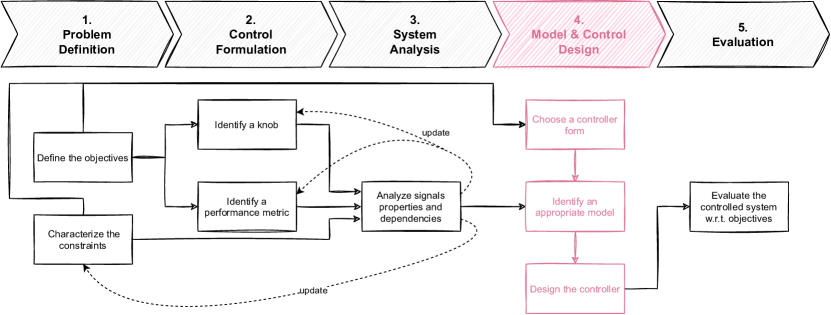
Figure 2: Methodological steps in using control theory for HPC systems. Step 4 (highlighted in pink) can be done independently by control experts.

The use of control theory tooling for computing systems is recent, especially in HPC[27]. The community still lacks well-defined and accepted models. Needed, therefore, is a methodology to identify and construct models upon which controllers can be designed. Fig. 2 depicts the method used for this work. It adapts the traditional workflow of control theory[11], by explicitly considering the upstream work of defining the problem and translating it to a control-friendly formulation in five main steps:

(1) Problem definition

First, the objectives have to be settled and the challenging characteristics and constraints identified. Here the problem definition naturally results from Sections 1 and 2. It consists of sustaining the application execution time while reducing energy usage as much as possible. This is challenging given the following constraints: applications have unpredictable phases with exogenous limits on progress, progress metrics are application-specific, processor characteristics and performance are various, power actuators have a limited accuracy and are distributed on all packages, and thermal considerations induce nonlinearities.

(2) Control formulation

The objectives are then translated into suitable control signals: these are knobs that enable one to act on the system at runtime and performance metric(s) to monitor the system’s behavior. They need to be measurable or computable on the fly. For example, the RAPL powercap value and the application progress are such signals.

(3) System analysis

The knobs are then analyzed to assess the impact of both their levels and the change of their levels on the performance signals during the execution time (cf. Section 4.3). The control formulation may be updated after this analysis to ease the control development (select adequate sampling time, modify signals with logarithmic scales, offsets). New constraints may be highlighted, such as the number of packages in a node.

(4) Model and control design

Once the relationships between signals and the system’s behavior have been identified, the control theory toolbox may be used[15]. According to the objectives and the identified system characteristics challenging them, a controller form is chosen, a PI controller in this case. An adequate model is identified from experimental data, such as a first-order dynamical model (see Section 4.4), and then used to design and tune the controller, following the pole placement method here (see Section 4.5).

(5) Evaluation

Eventually, the controlled system is evaluated with respect to the objectives (cf. Section 5). In this paper we are interested in evaluating the energy reduction and execution time increase according to the maximal allowed degradation given to the controller.

4 Model and Controller Development

We defined the problem under study in Sections 1 and 2. Following the method described in Section 3, we now focus on formulating it as a control problem, analyzing the system to derive a model and design a controller (Steps 2 to 4). As depicted in Fig. 2, the early steps are refined in an iterative process with respect to the analysis results. Since the analysis of the system requires observing the behavior of the system, we first describe the experimental setup.

4.1 Experimental Setup

Platform

All experiments were conducted on the Grid’5000 testbed. We ran the experiments on nodes of three different clusters: gros, dahu, and yeti. These clusters were chosen because their nodes have modern Intel CPUs and a varying number of sockets. We list in Table 1 the main characteristics of the clusters. The exact specifications of the clusters are available on the Grid’5000 wiki.

Cluster	CPU	Cores/CPU	Sockets	RAM $\left[$\mathrm{GiB}$\right]$
gros	Xeon Gold 5220	18	1	96
dahu	Xeon Gold 6130	16	2	192
yeti	Xeon Gold 6130	16	4	768

Table 1: Hardware characteristics of Grid’5000 clusters used for the experiments.

Software stack

All experiments ran on a deployed environment with a custom image. The deployed environment is a minimal GNU/Linux Debian 10.7 “buster” with kernel 4.19.0-13-amd64. The management of applications and resources was implemented within the Argo NRM, a resource management framework developed at Argonne National Laboratory. We used the version tagged as expe-0.6 for this work. NRM and benchmarks are packaged with the Nix functional package manager[8]: we rely on a multiuser installation of Nix version 2.3.10.

Benchmark

All experiments involved execution of the STREAM benchmark[17]. STREAM is chosen as it is representative of memory-bound phases of applications and shows a stable behavior. STREAM is also easy to modify into an iterative application, which allows computation of the progress metric by reporting heartbeats. We used version 5.10 with a problem size set to $33554432$ and $10000\text{\,}\mathrm{i}\mathrm{t}\mathrm{e}\mathrm{r}\mathrm{a}\mathrm{t}\mathrm{i}\mathrm{o}\mathrm{n}\mathrm{s}$, further adapted to run in a way that progress can be tracked: its 4 kernels ran a configurable number of times in a loop, with a heartbeat being reported to the NRM each time the loop completed (after one run of the four kernels).

Characterization vs. Evaluation setup

Although the hardware and software stack remain the same, we need to distinguish characterization and evaluation experiments. For the analysis of the system (characterization), we observe the behavior of the system, and the resource manager follows a predefined plan. This contrasts with the evaluation setup, where the resource manager reacts to the system’s behavior. From the control theory perspective, the former setup is an open-loop system while the latter is a closed-loop system.

4.2 Control Formulation

The power actuator is RAPL’s power limit denoted $\text{pcap}(t_{i})$. To define a progress metric, we aggregate the heartbeats that the application generates at times $t_{k}$ (see Section 2.1) into a signal synchronized with the power actuator. The progress metric at $t_{i}$ is formally defined as the median of the heartbeats arrival frequencies since the last sampling time $t_{i-1}$:

$$\text{progress}(t_{i})=\underset{\forall k,\,t_{k}\in\left[t_{i-1},t_{i}\right[}{\operatorname{median}}\left(\frac{1}{t_{k}-t_{k-1}}\right)$$ (1)

A central tendency indicator, in particular the median, was selected to be robust to extreme values so as to provide the controller with a smooth signal. The primary performance objective is based on the application’s execution time, while for control purposes a runtime metric is needed.

Before further control development, let us ensure the correlation between the two. We compute the Pearson correlation coefficient[18] between the progress metric and execution time. The Pearson value is respectively $0.97$, $0.80$, and $0.80$ on gros, dahu, and yeti clusters when computed by using static characterization data (constant powercap over the whole benchmark duration; see Section 4.4.1). The high correlation results validate the progress definition choice, with a notably strong correlation on the 1-socket cluster.

4.3 System Analysis

The analysis phase assesses the trustworthiness of the power actuator and progress sensor and measures how powercap levels impact progress.

During the benchmark execution, the powercap is gradually increased by steps of $20\text{\,}\mathrm{W}$ on the clusters’ reasonable power range (i.e., from $40\text{\,}\mathrm{W}120\text{\,}\mathrm{W}$), and the progress is measured; see Fig. 3. First, we see that the measured power never corresponds to the requested level and that the error increases with the powercap value. The RAPL powercap actuator accuracy is poor[7] and will have to be taken into account. The progress variations follow the power ones, whereas the higher the power level, the less a power increase impacts the progress. This highlights the nonlinearity of the power-to-progress dynamical system, with a saturation effect at high power values. The saturation results from the memory-boundedness of the application: at high power levels, the processor power is not limiting performance as memory is. The power level at which the saturation appears is related to the processors’ thermal design power.We also note that the more packages there are in the cluster, the noisier the progress. Additionally, Fig. 3(c) illustrates that the progress is impacted by external factors, since in this run the power signal in itself does not explain the progress plateau from $20\text{\,}\mathrm{s}60\text{\,}\mathrm{s}$ and the drop to $10\text{\,}\mathrm{Hz}$ at $80\text{\,}\mathrm{s}$. This behavior is further discussed in Section 5.2.1.

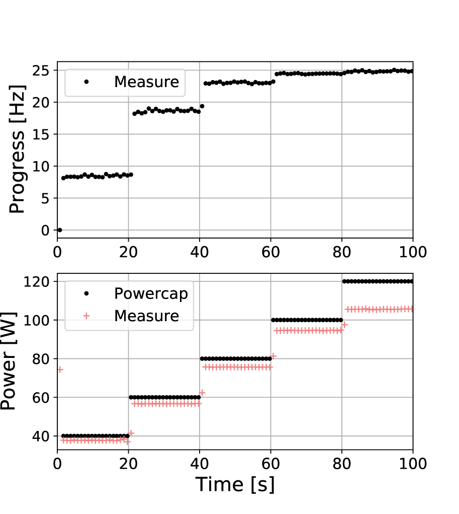
(a) gros cluster

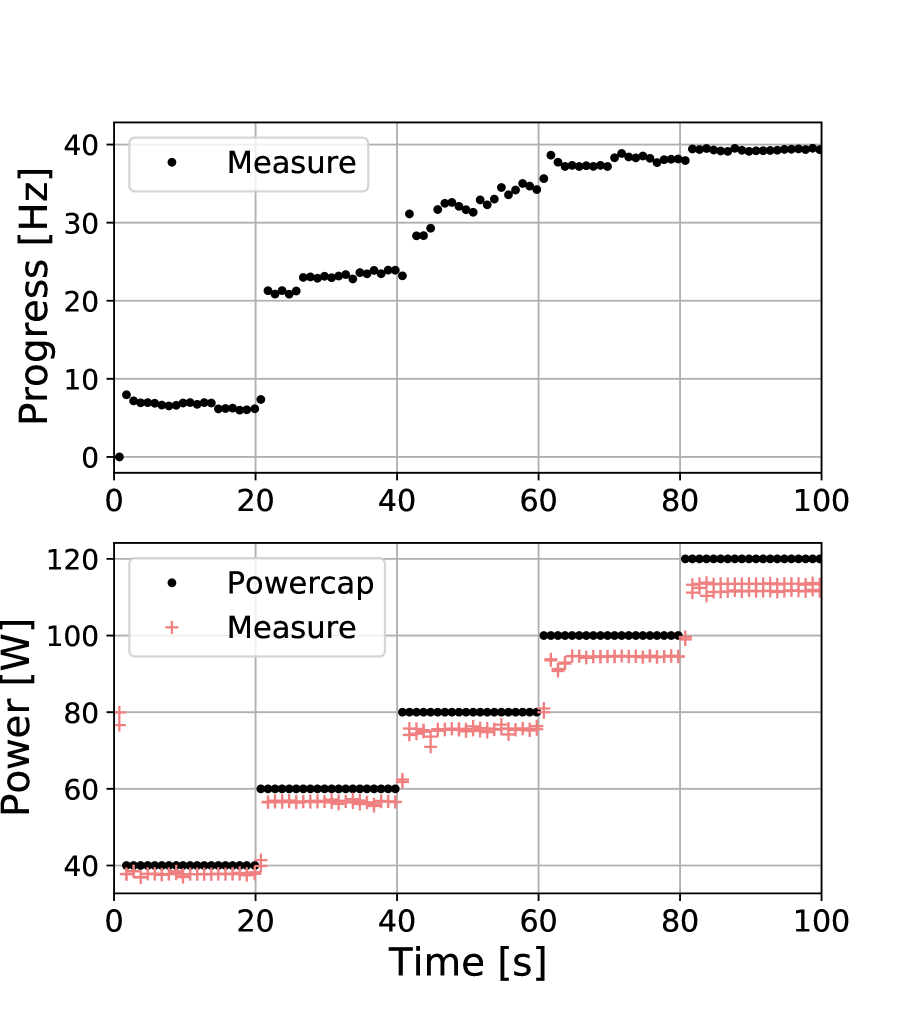
(b) dahu cluster

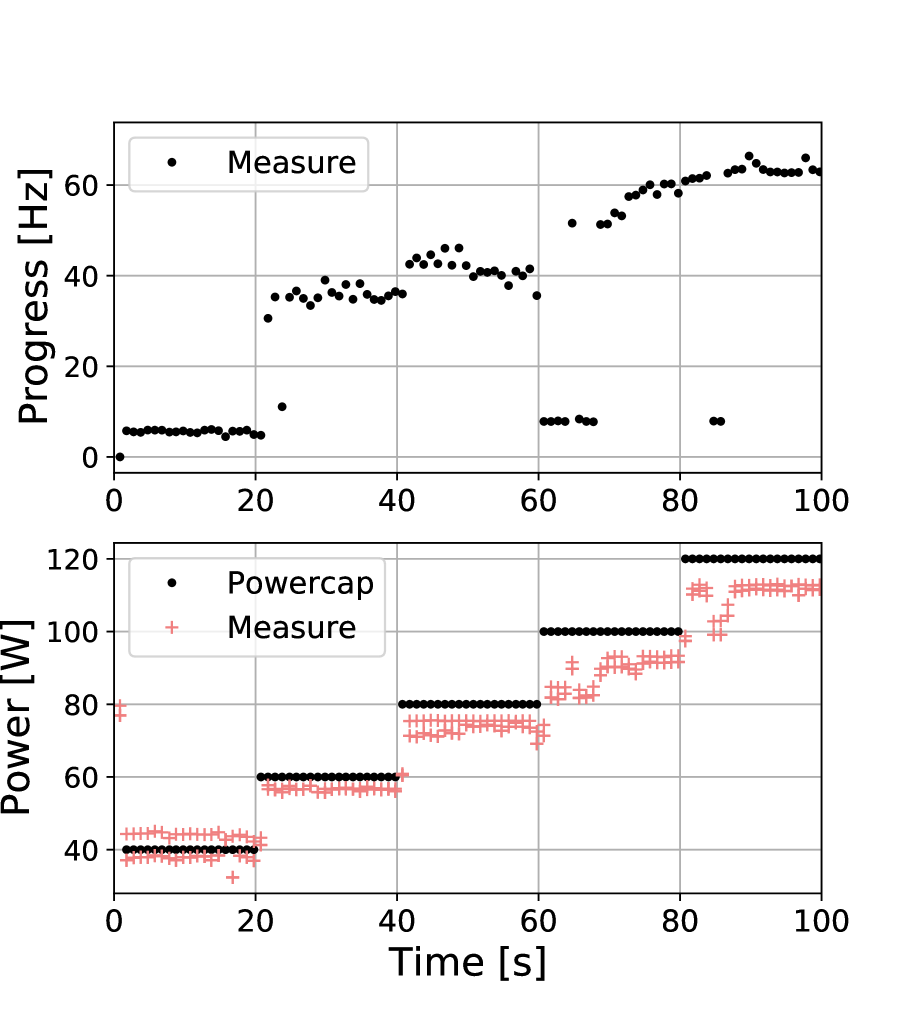
(c) yeti cluster

Figure 3: Impact of power changes on progress: the time perspective. Each sub-figure depicts a single representative execution.

In summary, this analysis shows that soundly tuning the power level enables application progress to be maintained while reducing the energy footprint. This highlights the need for runtime feedback to cope with external factors. Since all clusters show similar behavior, a common controller can be designed. Cluster-specific modeling will further enable leveraging of its parameters.

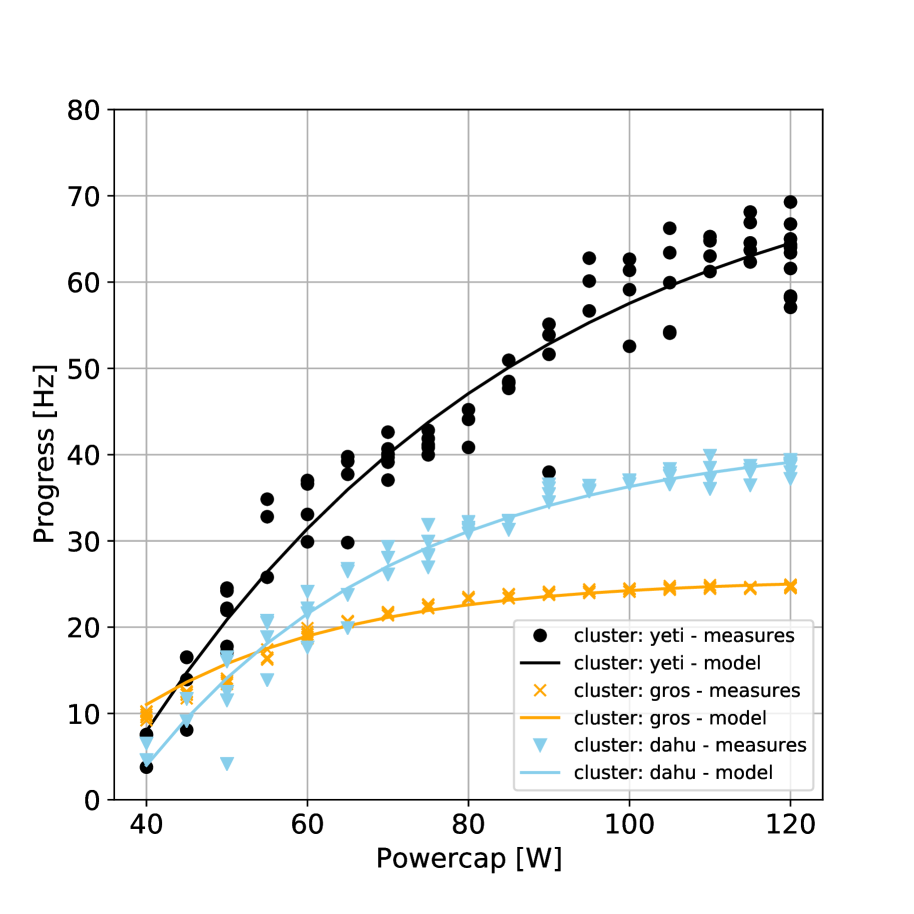
(a) From powercap to progress.

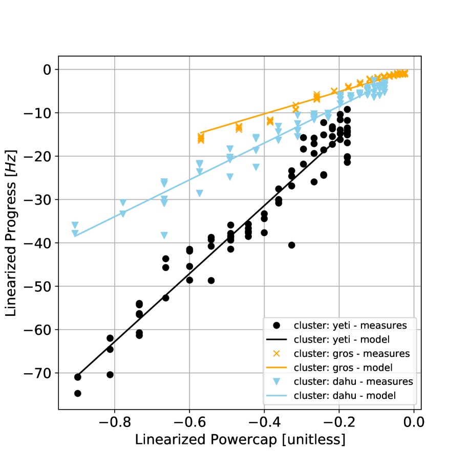
(b) Linearized model.

Figure 4: Static characteristic: modeling of time-averaged behavior. Each point depicts a single execution.

4.4 Modeling

A system model—namely, a set of equations linking the power and progress—is a first step toward a controller taking sound actions. This step needs to be performed only once per cluster to measure model parameters to tune the controller.

4.4.1 Static characteristic: averaged behavior.

The time-averaged relation between power and progress is first modeled in a so-called static characterization, in the sense that it considers stabilized situations. In Fig. 4(a), each data point corresponds to an entire benchmark execution where a constant powercap is applied (at the level reported on $x$-axis) and for which the progress signal is averaged ($y$-axis). We depict with different colors and markers the measures for the three clusters we use in this work. For each cluster, at least $68\text{\,}\mathrm{e}\mathrm{x}\mathrm{p}\mathrm{e}\mathrm{r}\mathrm{i}\mathrm{m}\mathrm{e}\mathrm{n}\mathrm{t}\mathrm{s}$ were run. Note that the curves are flattening, indicating the nonlinear behavior and saturation at large power previously identified.

Based on those experiments, a static model, linking the time-stabilized powercap to the progress is: $\text{progress}=K_{L}\left(1-e^{-\alpha\left(a\cdot\text{pcap}+b-\beta\right)}\right)$ where $a$ and $b$ parameters represent RAPL actuator accuracy on the cluster (slope and offset, resp.: $\text{power}=a\cdot\text{pcap}+b$), $\alpha$ and $\beta$ characterize the benchmark-dependent power-to-progress profile, and $K_{L}$ is the linear gain being both benchmark and cluster specific. The effective values of these parameters can be automatically found by using nonlinear least squares; they are reported in Table 2. The solid lines in Fig. 4(a) illustrate our model, which shows good accuracy ($0.83<R^{2}<0.95$).

Control formulation update.

Given the nonlinearity of Section 4.4.1, we simplify the control by linearizing the powercap and progress signals; see Fig. 4(b). The linearized version of a signal $\star$ is denoted by ${\star}_{L}$:

$${\text{pcap}}_{L}=-e^{-\alpha\left(a\cdot\text{pcap}+b-\beta\right)}\quad;\quad{\text{progress}}_{L}=\text{progress}-K_{L}$$ (2)

4.4.2 Dynamic perspective: modeling impact of power variations.

We now characterize the dynamics, that is, the effects of a change of the power level on the progress signal over time. First, the model form is selected. As a compromise between accuracy and simplicity, we opt for a first-order model[12]. It means that the prediction of the progress requires only one previous value of the measured progress and the enforced powercap level: ${\text{progress}}_{L}(t_{i+1})=f\left({\text{progress}}_{L}(t_{i}),{\text{pcap}}_{L}(t_{i})\right).$ Control theory provides a first-order model formulation based on the static characteristic gain $K_{L}$ and on a time constant $\tau$ characterizing the transient behavior:

$${\text{progress}}_{L}(t_{i+1})=\frac{K_{L}\Delta t_{i}}{\Delta t_{i}+\tau}\cdot{\text{pcap}}_{L}(t_{i})+\frac{\tau}{\Delta t_{i}+\tau}\cdot{\text{progress}}_{L}(t_{i})$$ (3)

where $\Delta t_{i}=t_{i+1}-t_{i}$. Based on experimental data, $\tau=$1\text{/}3\text{\,}\mathrm{Hz}$$ for all clusters.

4.5 Control Design

The control objective is given as a degradation factor $\epsilon$, that is, the tolerable loss of performance. The controller translates $\epsilon$ in a progress setpoint to track using the maximum progress ($\text{progress}_{\text{max}}$) estimated by using Section 4.4.1 with the cluster maximal power. A feedback PI controller is developed (see Section 2.2), setting the powercap proportionally to the progress error $e(t_{i})=(1-\epsilon)\cdot\text{progress}_{\text{max}}-\text{progress}(t_{i})$ and to the integral of this error (see Section 2.2):

$$\begin{split}{\text{pcap}}_{L}(t_{i})&=\left(K_{I}\Delta t_{i}+K_{P}\right)\cdot e(t_{i})-K_{P}\cdot e(t_{i-1})+{\text{pcap}}_{L}(t_{i-1})\end{split}$$ (4)

The parameters $K_{P}$ and $K_{I}$ are based both on the model parameters $K_{L}$ and $\tau$ and on a tunable parameter $\tau_{\text{obj}}$: $K_{P}={\tau}/{\left(K_{L}\cdot\tau_{\text{obj}}\right)}$ and $K_{I}={1}/{\left(K_{L}\cdot\tau_{\text{obj}}\right)}$, with $\tau_{\text{obj}}$ defining the desired dynamical behavior of the controlled system[3]. The controller is chosen to be nonaggressive, tuned with $\tau_{\text{obj}}=$10\text{\,}\mathrm{s}$>10\tau$. The powercap is computed from its linearized value by using Eq. 2.

5 Evaluation

The experimental setup has been described in Section 4.1. We evaluate here the performance of the model and controller designed in the preceding section using the memory-bound STREAM benchmark run on three clusters with varying number of sockets.

We recapitulate in Table 2 the values of the model and controller parameters. The model parameters $a$, $b$, $\alpha$, and $\beta$ have been fitted for each cluster with the static characterization experiments (cf. Fig. 4). The model parameters $K_{L}$ and $\tau$ and the controller parameter $\tau_{\text{obj}}$ have been chosen with respect to the system’s dynamic (cf. Fig. 3). These values have been used for the evaluation campaign.

Description	Notation	Unit	gros	dahu	yeti
RAPL slope	$a$	$\left[$\mathrm{1}$\right]$	0.83	0.94	0.89
RAPL offset	$b$	$\left[$\mathrm{W}$\right]$	7.07	0.17	2.91
	$\alpha$	$\left[${\mathrm{W}}^{-1}$\right]$	0.047	0.032	0.023
power offset	$\beta$	$\left[$\mathrm{W}$\right]$	28.5	34.8	33.7
linear gain	$K_{L}$	$\left[$\mathrm{Hz}$\right]$	25.6	42.4	78.5
time constant	$\tau$	$\left[$\mathrm{s}$\right]$	1/3	1/3	1/3
	$\tau_{\text{obj}}$	$\left[$\mathrm{s}$\right]$	10	10	10

Table 2: Model and controller parameters for each cluster.

5.1 Measure of the Model Accuracy

The presented model is not intended to perform predictions: it is used only for the controller tuning. However, we take a brief look at its accuracy. To do so, a random powercap signal is applied, with varying magnitude (from $40\text{\,}\mathrm{W}120\text{\,}\mathrm{W}$) and frequency (from ${10}^{-2}\text{\,}\mathrm{Hz}1\text{\,}\mathrm{Hz}$), and the benchmark progress is measured. For each cluster, at least 20 of such identification experiments were run. Figure 5 illustrates a single execution for each cluster, with the progress measure and its modeled value through time on the top plots and the powercap and power measures on the bottom ones. Visually, the modeling is fairly accurate, and the fewer the sockets, the less noisy the progress metric and the better the modeling. The average error is close to zero for all clusters. Nevertheless, our model performs better on clusters with few sockets (narrow distribution and short extrema).

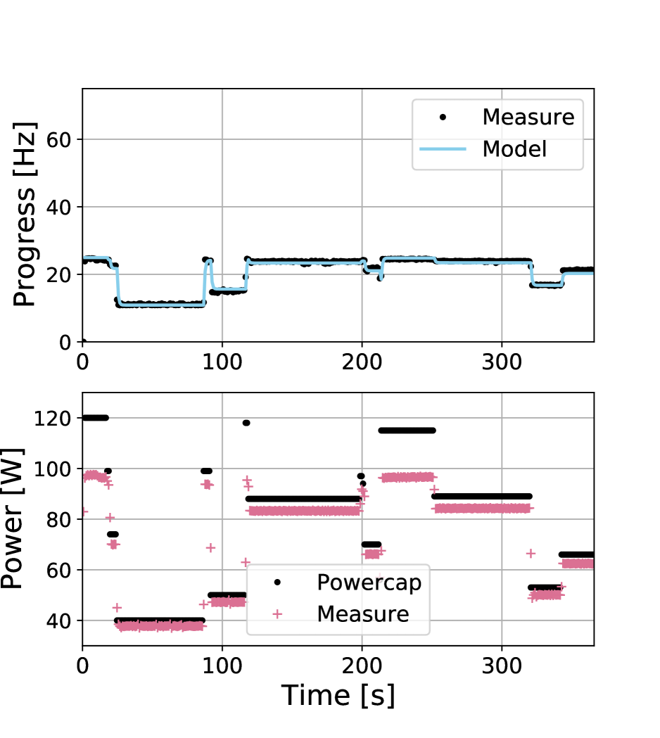
(a) gros cluster

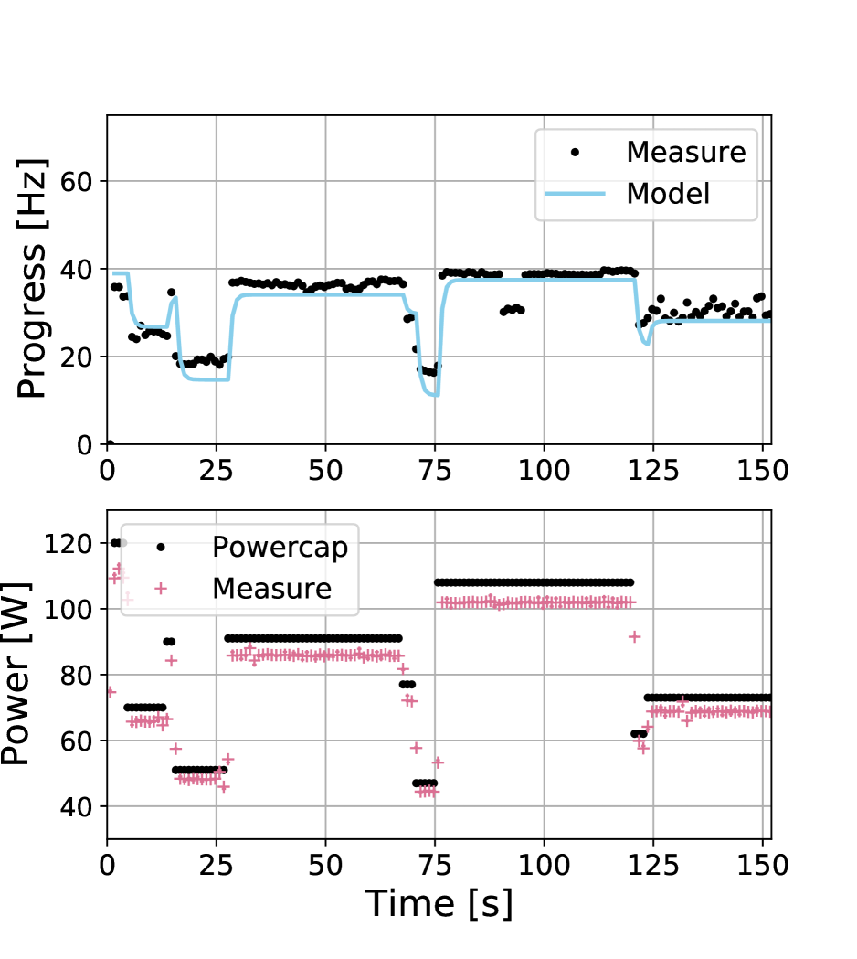
(b) dahu cluster

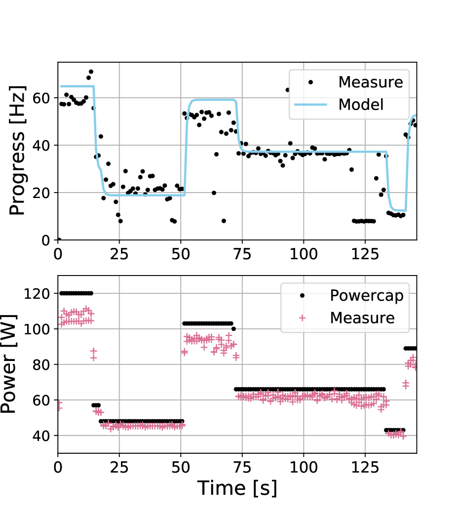
(c) yeti cluster

Figure 5: Modeling the time dynamics. Each sub-figure depicts a single representative execution.

5.2 Evaluation of the Controlled System

In this section we evaluate the behavior of the system when the controller reacts to the system’s evolution. Results are reported for different clusters with the controller required to reach a set of degradation factors ($\epsilon\in[0,0.5]$). Experiments are repeated 30 times for each combination of cluster and degradation value.

Figure 6(a) shows a typical controlled system behavior through time on the gros cluster. The initial powercap is set at its upper limit, and the controller smoothly decreases its value until progress reaches the objective level (15% degradation here). Note that the controlled system behavior shows neither oscillation nor degradation of the progress below the allowed value. We report in Fig. 6(b) the distribution of the tracking error: the difference between the progress setpoint chosen by the controller and the measured progress. The depicted distributions aggregate all experiments involving the controller. The distributions of the error for the gros and dahu clusters are unimodal, centered near 0 ($-0.21$ and $-0.60$, resp.) with a narrow dispersion ($1.8$ and $6.1$, resp.). On the other hand, the distribution of the error for the yeti cluster exhibits two modes: the second mode (located between $50\text{\,}\mathrm{Hz}60\text{\,}\mathrm{Hz}$) is due to the model limitations. For reasons to be investigated, the progress sometimes drops to about $10\text{\,}\mathrm{Hz}$ regardless of the requested power cap. This behavior is notably visible in Fig. 3(c) and is on a par with the observation that the more sockets a system has, the noisier it becomes.

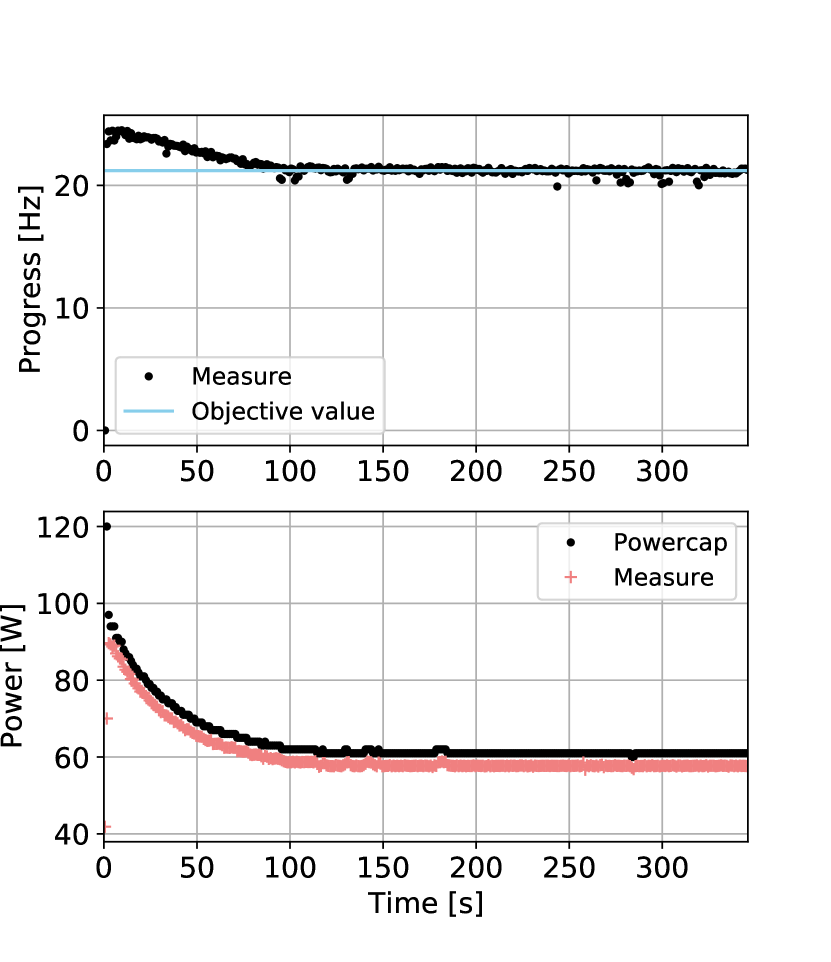
(a) Controlled system behavior: Progress and powercap trough time ($\epsilon=0.15$, gros cluster). Single representative execution.

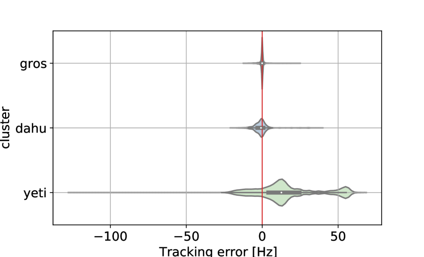
(b) Distribution of the tracking error per cluster. The sub-figure aggregates all executions run with the controller.

Figure 6: Evaluation of the controlled system.

The controller objective is to adapt the benchmark speed by adapting the powercap on the fly, meaning we are exploiting time-local behavior of the system. Nevertheless, we are interested in the global behavior of the benchmark, in other words, the total execution time and the total energy consumption. To this end, we assessed the performance of the controlled system with a post mortem analysis. We tested a total of twelve degradation levels ranging from $0.01$ to $0.5$, and ran each configuration a minimum of thirty times. Figure 7 depicts the total execution time and the total energy consumption for each tested degradation level $\epsilon$ in the time/energy space. The experiments unveil a Pareto front for the gros and dahu clusters for degradation levels ranging from $0\text{\,}\mathrm{\char 37\relax}15\text{\,}\mathrm{\char 37\relax}$ (Figs. 7(a) and 7(b)): this indicates the existence of a family of trade-offs to save energy. For example, the $\epsilon=0.1$ degradation level on the gros cluster is interesting because it allows, on average, saving $22\text{\,}\mathrm{\char 37\relax}$ energy at the cost of a $7\text{\,}\mathrm{\char 37\relax}$ execution time increase when compared with the baseline execution ($\epsilon=0$ degradation level). Note that degradation levels over $15\text{\,}\mathrm{\char 37\relax}$ are not interesting because the increase in the execution time negates the energy savings. The behavior on the yeti cluster is too noisy to identify interesting degradation levels. However, the proposed controller does not negatively impact the performance.

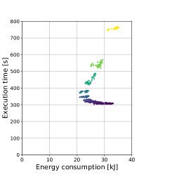
(a) gros cluster

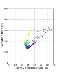
(b) dahu cluster

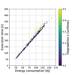
(c) yeti cluster

Figure 7: Execution time with respect to energy consumption. Color indicates the requested degradation level $\epsilon$. Each point depicts a single execution.

5.2.1 Discussion

The proposed controller has an easily configured behavior: the user has to supply only an acceptable degradation level. The controller relies on a simple model of the system, and it is stable on the gros and dahu clusters. The approach does, however, show its limits on the yeti cluster, since the model is unable to explain the sporadic drops to $10\text{\,}\mathrm{Hz}$ in the application’s progress. This is particularly visible on Fig. 3(c) between $60\text{\,}\mathrm{s}70\text{\,}\mathrm{s}$. Nevertheless, we observe that these events can be characterized by the wider gap between the requested powercap and the measured power consumption. We suspect that the number of packages and the NUMA architecture, or exogenous temperature events, are responsible for these deviations. Further investigations are needed to confirm this hypothesis. If it is confirmed, development of control strategies will be considered for integrating distributed actuation or temperature disturbance anticipation.

On the generalization to other benchmarks.

The use of STREAM benchmark is motivated by its stable memory-bound profile, and its ability to be instrumented with heartbeats—thanks to its straightforward design. Figures 5 and 3 illustrate this stability: while no powercap change occurs, performance is largely constant. The presented approach extends similarly for memory intensive phases of applications. We expect compute-bound phases to show a different (simpler) power to progress profile (Fig. 4), less amenable to optimization. Indeed, every power increase should improve performance, even for high powercap values. Furthermore, with such linear behavior, modeling will have to be recomputed, and controller parameters updated. Overall, controlling an application with varying resource usage patterns thus requires adaptation—a control technique implying automatic tuning of the controller parameters—to handle powercap-to-progress behavior transitions between phases. It is a natural direction of research for future work.

6 Related Work

On power regulation in HPC.

A large body of related work seeks to optimize performance or control energy consumption on HPC systems using a wide range of control knobs[4, 9, 19, 20]. Most of these methods, however, target a different objective from our work or are based either on static schemes used at the beginning of a job or on simple loops without formal performance guarantees. This is also the case for GeoPM[10], the most prominent available power management infrastructure for HPC systems. An open source framework designed by Intel, GeoPM uses the same actuator than as our infrastructure (RAPL) does but with application-oblivious monitoring (PMPI or OMPT) capabilities.

On using control theory for power regulation.

Control-theory-based approaches to power regulation focus mainly on web servers[1], clouds[28], and real-time systems[13] applications. They typically leverage DVFS[2] as an actuator and formulate their objectives in terms of latency. Controllers are adaptive, with an update mechanism to cope with unmodeled external disturbances. The present work stands out for two reasons. First, it uses Intel’s RAPL mechanism, a unified architecture-agnostic and future-proof solution, to leverage power. Moreover, we do not consider applications with predefined latency objectives but instead focus on the science performed by HPC applications, based on a heartrate progress metric. Other works similarly use RAPL in web servers[16] and real-time systems[14] contexts and non-latency-based performance metrics[26]. To the best of our knowledge, however, we present the first control theory approach to power regulation using RAPL for HPC systems.

7 Conclusion

We address the problem of managing energy consumption in complex heterogeneous HPC by focusing on the potential of dynamically adjusting power across compute elements to save energy with limited and controllable impact on performance. Our approach involves using control theory, with a method adapted to HPC systems, and leads to identification and controller design for the targeted system. Experimental validation shows good results for systems with lower numbers of sockets running a memory-bound benchmark. We identify limiting aspects of our method and areas for further study, such as integrating measures of the temperature or extending the control to heterogeneous devices.

Acknowledgments and Data Availability Statement

Experiments presented in this paper were carried out using the Grid’5000 testbed, supported by a scientific interest group hosted by Inria and including CNRS, RENATER and several Universities as well as other organizations (see https://www.grid5000.fr). Argonne National Laboratory’s work was supported by the U.S. Department of Energy, Office of Science, Advanced Scientific Computer Research, under Contract DE-AC02-06CH11357. This research was supported by the Exascale Computing Project (17-SC-20-SC), a collaborative effort of the U.S. Department of Energy Office of Science and the National Nuclear Security Administration. This research is partially supported by the NCSA-Inria-ANL-BSC-JSC-Riken-UTK Joint-Laboratory for Extreme Scale Computing (JLESC, https://jlesc.github.io/).

The datasets and code generated and analyzed during the current study are available in the Figshare repository: https://doi.org/10.6084/m9.figshare.14754468[5].

References

- [1] Abdelzaher, T., et al.: Introduction to Control Theory And Its Application to Computing Systems. In: Performance Modeling and Engineering, pp. 185–215. Springer (2008). https://doi.org/10.1007/978-0-387-79361-0_7
- [2] Albers, S.: Algorithms for Dynamic Speed Scaling. In: STACS. LIPIcs, vol. 9, pp. 1–11. Schloss Dagstuhl - Leibniz-Zentrum für Informatik (2011). https://doi.org/10.4230/LIPIcs.STACS.2011.1
- [3] Åström, K.J., Hägglund, T.: PID Controllers: Theory, Design, and Tuning. International Society of Automation, second edn. (1995)
- [4] Bhalachandra, S., et al.: Using Dynamic Duty Cycle Modulation to Improve Energy Efficiency in High Performance Computing. In: IPDPS Workshops. pp. 911–918. IEEE (May 2015). https://doi.org/10.1109/IPDPSW.2015.144
- [5] Cerf, S., et al.: Artifact and instructions to generate experimental results for the Euro-Par 2021 paper: ”Sustaining Performance While Reducing Energy Consumption: A Control Theory Approach” (Aug 2021). https://doi.org/10.6084/m9.figshare.14754468
- [6] David, H., et al.: RAPL: Memory Power Estimation and Capping. In: ISLPED. pp. 189–194. ACM (2010). https://doi.org/10.1145/1840845.1840883
- [7] Desrochers, S., et al.: A Validation of DRAM RAPL Power Measurements. In: MEMSYS. pp. 455–470. ACM (Oct 2016). https://doi.org/10.1145/2989081.2989088
- [8] Dolstra, E., et al.: Nix: A Safe and Policy-Free System for Software Deployment. In: LISA. pp. 79–92. USENIX (2004), http://www.usenix.org/publications/library/proceedings/lisa04/tech/dolstra.html
- [9] Dutot, P., et al.: Towards Energy Budget Control in HPC. In: CCGrid. pp. 381–390. IEEE / ACM (May 2017). https://doi.org/10.1109/CCGRID.2017.16
- [10] Eastep, J., et al.: Global Extensible Open Power Manager: A Vehicle for HPC Community Collaboration on Co-Designed Energy Management Solutions. In: ISC. Lecture Notes in Computer Science, vol. 10266, pp. 394–412. Springer (Jun 2017). https://doi.org/10.1007/978-3-319-58667-0_21
- [11] Filieri, A., et al.: Control Strategies for Self-Adaptive Software Systems. ACM Trans. Auton. Adapt. Syst. 11(4), 24:1–24:31 (Feb 2017). https://doi.org/10.1145/3024188
- [12] Hellerstein, J.L., et al.: Feedback Control of Computing Systems. Wiley (2004). https://doi.org/10.1002/047166880X
- [13] Imes, C., et al.: POET: A Portable Approach to Minimizing Energy Under Soft Real-time Constraints. In: RTAS. pp. 75–86. IEEE (Apr 2015). https://doi.org/10.1109/RTAS.2015.7108419
- [14] Imes, C., et al.: CoPPer: Soft Real-time Application Performance Using Hardware Power Capping. In: ICAC. pp. 31–41. IEEE (Jun 2019). https://doi.org/10.1109/ICAC.2019.00015
- [15] Levine, W.S.: The Control Handbook (three volume set). CRC Press, second edn. (2011). https://doi.org/10.1201/9781315218694
- [16] Lo, D., et al.: Towards Energy Proportionality for Large-Scale Latency-Critical Workloads. In: ISCA. pp. 301–312. IEEE (Jun 2014). https://doi.org/10.1109/ISCA.2014.6853237
- [17] McCalpin, J.D.: Memory Bandwidth and Machine Balance in Current High Performance Computers. IEEE Computer Society Technical Committee on Computer Architecture (TCCA) Newsletter pp. 19–25 (Dec 1995)
- [18] Montgomery, D.C., Runger, G.C.: Applied Statistics and Probability for Engineers. Wiley, seventh edn. (Jan 2018)
- [19] Orgerie, A., et al.: Save Watts in your Grid: Green Strategies for Energy-Aware Framework in Large Scale Distributed Systems. In: ICPADS. pp. 171–178. IEEE (Dec 2008). https://doi.org/10.1109/ICPADS.2008.97
- [20] Petoumenos, P., et al.: Power Capping: What Works, What Does Not. In: ICPADS. pp. 525–534. IEEE (Dec 2015). https://doi.org/10.1109/ICPADS.2015.72
- [21] Ramesh, S., et al.: Understanding the Impact of Dynamic Power Capping on Application Progress. In: IPDPS. pp. 793–804. IEEE (May 2019). https://doi.org/10.1109/IPDPS.2019.00088
- [22] Reis, V., et al.: Argo Node Resource Manager. https://www.mcs.anl.gov/research/projects/argo/overview/nrm/ (2021)
- [23] Rotem, E., et al.: Power-Management Architecture of the Intel Microarchitecture Code-Named Sandy Bridge. IEEE Micro 32(2), 20–27 (2012). https://doi.org/10.1109/MM.2012.12
- [24] Rountree, B., et al.: Beyond DVFS: A First Look at Performance under a Hardware-Enforced Power Bound. In: IPDPS Workshops. pp. 947–953. IEEE (2012). https://doi.org/10.1109/IPDPSW.2012.116
- [25] Rutten, É., et al.: Feedback Control as MAPE-K Loop in Autonomic Computing. In: Software Engineering for Self-Adaptive Systems. Lecture Notes in Computer Science, vol. 9640, pp. 349–373. Springer (2017). https://doi.org/10.1007/978-3-319-74183-3_12
- [26] Santriaji, M.H., Hoffmann, H.: GRAPE: Minimizing Energy for GPU Applications with Performance Requirements. In: MICRO. pp. 16:1–16:13. IEEE (Oct 2016). https://doi.org/10.1109/MICRO.2016.7783719
- [27] Stahl, E., et al.: Towards a control-theory approach for minimizing unused grid resources. In: AI-Science@HPDC. pp. 4:1–4:8. ACM (2018). https://doi.org/10.1145/3217197.3217201
- [28] Zhou, Y., et al.: CASH: Supporting IaaS Customers with a Sub-core Configurable Architecture. In: ISCA. pp. 682–694. IEEE (Jun 2016). https://doi.org/10.1109/ISCA.2016.65