Deep Network Approximation: Achieving Arbitrary Accuracy with Fixed Number of Neurons

Abstract

This paper develops simple feed-forward neural networks that achieve the universal approximation property for all continuous functions with a fixed finite number of neurons. These neural networks are simple because they are designed with a simple, computable, and continuous activation function $\sigma$ leveraging a triangular-wave function and the softsign function. We first prove that $\sigma$-activated networks with width $36d(2d+1)$ and depth $11$ can approximate any continuous function on a $d$-dimensional hypercube within an arbitrarily small error. Hence, for supervised learning and its related regression problems, the hypothesis space generated by these networks with a size not smaller than $36d(2d+1)\times 11$ is dense in the continuous function space $C([a,b]^{d})$ and therefore dense in the Lebesgue spaces $L^{p}([a,b]^{d})$ for $p\in[1,\infty)$. Furthermore, we show that classification functions arising from image and signal classification are in the hypothesis space generated by $\sigma$-activated networks with width $36d(2d+1)$ and depth $12$ when there exist pairwise disjoint bounded closed subsets of $\mathbb{R}^{d}$ such that the samples of the same class are located in the same subset. Finally, we use numerical experimentation to show that replacing the rectified linear unit (ReLU) activation function by ours would improve the experiment results.

Keywords: universal approximation property, fixed-size neural network, classification function, periodic function, nonlinear approximation

1 Introduction

Deep neural networks have been widely used in data science and artificial intelligence. Their tremendous successes in various applications have motivated extensive research to establish the theoretical foundation of deep learning. Understanding the approximation capacity of deep neural networks is one of the keys to revealing the power of deep learning. The most basic layers of deep neural networks are nonlinear functions as the composition of an affine linear transform and a nonlinear activation function. The composition of these simple nonlinear functions can generate a complicated deep neural network with powerful approximation capacity, which is the key difference from classic approximation tools. In this paper, we show that the hypothesis space of deep neural networks generated from the composition of $11$ such simple nonlinear functions is dense in the continuous function space $C([a,b]^{d})$ when the affine linear transforms are parameterized with ${\mathcal{O}}(d^{2})$ non-zero parameters in total and the nonlinear activation function is constructed from a simple triangular-wave function and the softsign function.

1.1 Main Results

One of the key elements of a neural network is its activation functions. Searching for simple activation functions enabling powerful approximation capacity of neural networks is an important mathematical problem that probably originated in the Kolmogorov superposition theorem (KST) (Kolmogorov, 1957) for Hilbert’s 13-th problem, where a two-hidden-layer neural network with ${\mathcal{O}}(d)$ neurons and complicated activation functions depending on the target functions are constructed to represent an arbitrary function in $C([0,1]^{d})$. Since then, whether simple and computable activation functions independent of the target function exist to make the space of neural networks with ${\mathcal{O}}(d)$ neurons dense in $C([0,1]^{d})$ or even equal to $C([0,1]^{d})$ has been an open problem. A function $\varrho:\mathbb{R}\to\mathbb{R}$ is said to be a universal activation function (UAF) if the function space generated by $\varrho$-activated networks with $C_{\varrho,d}$ neurons is dense in $C([0,1]^{d})$, where $C_{\varrho,d}$ is a constant determined by $\varrho$ and $d$. That is, if $\varrho$ is a UAF, then $\varrho$-activated networks with $C_{\varrho,d}$ neurons can approximate any continuous function within an arbitrary error on $[0,1]^{d}$ by only adjusting the parameters.

In this paper, we first construct a simple and computable example of UAFs. As a typical and simple UAF, this activation function is called elementary universal activation function (EUAF), and the corresponding networks are called EUAF networks. Then, we prove that the function space generated by EUAF networks with ${\mathcal{O}}(d^{2})$ neurons is dense in $C([a,b]^{d})$. Furthermore, it is shown that EUAF networks with ${\mathcal{O}}(d^{2})$ neurons can exactly represent $d$-dimensional classification functions.

While a good activation function should be simple and numerically implementable, the neural network activated by it should be able to approximate continuous functions well with a manageable size. Considering these requirements and motivated by previous works (Yarotsky and Zhevnerchuk, 2020; Shen et al., 2021a, b), the activation function to be chosen should have appropriate nonlinearity, periodicity, and the capacity to reproduce step functions. It is challenging to find a single activation function with all these properties. Here, we propose an activation function with all required properties by using two simple functions $\sigma_{1}$ and $\sigma_{2}$ defined below.

Let $\sigma_{1}$ be the continuous triangular-wave function with period $2$, i.e.,

$$\sigma_{1}(x)\coloneqq|x|\quad\textnormal{for any $x\in[-1,1]$}$$

and $\sigma_{1}(x+2)=\sigma_{1}(x)$ for any $x\in\mathbb{R}$. Alternatively, $\sigma_{1}$ can also be written as:

$$\sigma_{1}(x)=\big{|}x-2\lfloor\tfrac{x+1}{2}\rfloor\big{|}\quad\textnormal{for any $x\in\mathbb{R}$, \quad where $\lfloor\cdot\rfloor$ is the floor function.}$$

Clearly, $\sigma_{1}$ is periodic and $x-\sigma_{1}(x)$ is a continuous variant of the floor function as desired.

To introduce high nonlinearity, let $\sigma_{2}$ be the softsign activation function commonly used in machine learning (Turian et al., 2009; Le and Zuidema, 2015):

$$\sigma_{2}(x)\coloneqq\frac{x}{|x|+1}\quad\textnormal{for any $x\in\mathbb{R}$}.$$

Then the activation function $\sigma$ is defined as:

$$\sigma(x)\coloneqq\begin{cases}\sigma_{1}(x)&\textnormal{for}\ x\in[0,\infty),\\ \sigma_{2}(x)&\textnormal{for}\ x\in(-\infty,0).\\ \end{cases}$$ (1)

See an illustration of $\sigma$ in Figure 1. This activation function $\sigma$ is used to construct powerful neural networks in this paper.

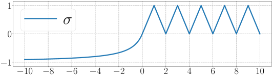
Figure 1: An illustration of $\sigma$ on $[-10,10]$.

As we shall see later, the periodicity of the triangular-wave function $\sigma_{1}$ and the (high) nonlinearity of the softsign function $\sigma_{2}$ play crucial roles in the proofs of our main results. One may find more details Section 2.2, which provides the ideas of proving our main results. Observe that $\sigma_{1}$ is an even function and $\sigma_{2}$ is an odd function, i.e., $\sigma(x)=\sigma_{1}(x)=\sigma_{1}(-x)$ for any $x\geq 0$ and $-\sigma(-x)=-\sigma_{2}(-x)=\sigma_{2}(x)$ for any $x\geq 0$. This implies that $\sigma(x)$ and $-\sigma(-x)$ with $x\geq 0$ have both required periodicity and nonlinearity features and play the same roles as $\sigma_{1}(x)$ and $\sigma_{2}(x)$, respectively. These requirements lead to our choice of $\sigma$ as the activation function. If allowed to be more complicated, one can design many other UAFs satisfying stronger requirements for various applications. For example, the idea of designing a $C^{s}$ UAF is given in Section 4.1 and a sigmoidal UAF (see Figure 8) is constructed in Section 4.2.

With the activation function $\sigma$ in hand, let us introduce the network (architecture) using $\sigma$ as the activation function, called $\sigma$-activated network (architecture). To be precise, a $\sigma$-activated network with a (vector) input ${\bm{x}}\in\mathbb{R}^{d}$, an output $\Phi({\bm{x}},{\bm{\theta}})\in\mathbb{R}$, and $L\in\mathbb{N}^{+}$ hidden layers can be briefly described as follows:

$$\bm{x}=\widetilde{\bm{h}}_{0}\mathop{\vbox{\hbox{\scalebox{1.0}[1.0]{ \leavevmode\hbox to41.11pt{\vbox to16.57pt{\text{[drawing]}}}}}}}^{\bm{A}_{0},\ \bm{b}_{0}}_{{\bm{\mathcal{L}}}_{0}}\bm{h}_{1}\mathop{\vbox{\hbox{\scalebox{1.0}[1.0]{ \leavevmode\hbox to23.3pt{\vbox to0.72pt{\text{[drawing]}}}}}}}^{\sigma}\widetilde{\bm{h}}_{1}\quad{\cdots}\quad\mathop{\vbox{\hbox{\scalebox{1.0}[1.0]{ \leavevmode\hbox to51.76pt{\vbox to0.72pt{\text{[drawing]}}}}}}}^{\bm{A}_{L-1},\ \bm{b}_{L-1}}_{{\bm{\mathcal{L}}}_{L-1}}\bm{h}_{L}\mathop{\vbox{\hbox{\scalebox{1.0}[1.0]{ \leavevmode\hbox to23.3pt{\vbox to0.72pt{\text{[drawing]}}}}}}}^{\sigma}\widetilde{\bm{h}}_{L}\mathop{\vbox{\hbox{\scalebox{1.0}[1.0]{ \leavevmode\hbox to39.98pt{\vbox to0.72pt{\text{[drawing]}}}}}}}^{\bm{A}_{L},\ \bm{b}_{L}}_{{\bm{\mathcal{L}}}_{L}}\bm{h}_{L+1}=\Phi(\bm{x},{\bm{\theta}}),$$ (2)

where $N_{0}=d\in\mathbb{N}^{+}$, $N_{1},N_{2},{\cdots},N_{L}\in\mathbb{N}^{+}$, $N_{L+1}=1$, $\bm{A}_{i}\in\mathbb{R}^{N_{i+1}\times N_{i}}$ and $\bm{b}_{i}\in\mathbb{R}^{N_{i+1}}$ are the weight matrix and the bias vector in the $i$-th affine linear transform ${\bm{\mathcal{L}}}_{i}$, respectively, i.e.,

$$\bm{h}_{i+1}=\bm{A}_{i}\cdot\widetilde{\bm{h}}_{i}+\bm{b}_{i}\eqqcolon{\bm{\mathcal{L}}}_{i}(\widetilde{\bm{h}}_{i})\quad\textnormal{for $i=0,1,{\cdots},L$}$$

and

$$\widetilde{{h}}_{i,j}=\sigma({h}_{i,j})\quad\textnormal{for $j=1,2,{\cdots},N_{i}$ and $i=1,2,{\cdots},L$.}$$

Here, $\widetilde{{h}}_{i,j}$ and ${h}_{i,j}$ are the $j$-th entries of $\widetilde{\bm{h}}_{i}$ and $\bm{h}_{i}$, respectively, for $j=1,2,{\cdots},N_{i}$ and $i=1,2,{\cdots},L$. ${\bm{\theta}}$ is a fattened vector consisting of all parameters in $\bm{A}_{0},{\bm{b}}_{0},\bm{A}_{1},{\bm{b}}_{1},{\cdots},\bm{A}_{L},{\bm{b}}_{L}$.

With a slight abuse of notation, $\sigma$ can be applied to a vector elementwisely, i.e., given any $k\in\mathbb{N}^{+}$,

$$\sigma({\bm{y}})=\big{[}\sigma(y_{1}),\,\sigma(y_{2}),\,{\cdots},\,\sigma(y_{k})\big{]}^{T}\quad\textnormal{ for any ${\bm{y}}=[y_{1},y_{2},{\cdots},y_{k}]^{T}\in\mathbb{R}^{k}$.}$$

Then $\Phi$ can be represented in a form of function compositions as follows:

$$\Phi({\bm{x}},{\bm{\theta}})={\bm{\mathcal{L}}}_{L}\circ\sigma\circ{\bm{\mathcal{L}}}_{L-1}\circ\,\ {\cdots}\,\ \circ\sigma\circ{\bm{\mathcal{L}}}_{1}\circ\sigma\circ{\bm{\mathcal{L}}}_{0}({\bm{x}})\quad\textnormal{for any ${\bm{x}}\in\mathbb{R}^{d}$}.$$

Given $N,L\in\mathbb{N}^{+}$, let $\Phi_{N,L}({\bm{x}},{\bm{\theta}})$ denote the $\sigma$-activated network architecture $\Phi({\bm{x}},{\bm{\theta}})$ in Equation (2) with $N_{1}=N_{2}={\cdots}=N_{L}=N$. Let

$$W=W_{d,N,L}=d\times N+N\ +\ (N\times N+N)\times(L-1)\ +\ N\times 1+1={\mathcal{O}}(dN+N^{2}L)$$

be the total number of parameters in $\Phi_{N,L}({\bm{x}},{\bm{\theta}})$, i.e., ${\bm{\theta}}\in\mathbb{R}^{W}$.

Define the hypothesis space $\mathscr{H}_{d}(N,L)$ as the function space generated by $d$-input EUAF networks with width $N$ and depth $L$, i.e.,

$$\mathscr{H}_{d}(N,L)\coloneqq\Big{\{}\phi:\phi({\bm{x}})=\Phi_{N,L}({\bm{x}},{\bm{\theta}})\textnormal{ for any ${\bm{x}}\in\mathbb{R}^{d}$},\quad{\bm{\theta}}\in\mathbb{R}^{W}\Big{\}}.$$ (3)

Let $C([a,b]^{d})$ be the space of all continuous functions $f:[a,b]^{d}\to\mathbb{R}$ with the maximum norm. Our first main result, Theorem 1 below, shows that EUAF networks with a fixed size ${\mathcal{O}}(d^{2})$ enjoy the universal approximation property by only adjusting their parameters.

Theorem 1.

Let $f\in C([a,b]^{d})$ be a continuous function and ${\mathscr{H}}_{d}(N,L)$ be the hypothesis space defined in Equation (3) with $N=36d(2d+1)$ and $L=11$. Then, for an arbitrary $\varepsilon>0$, there exists $\phi\in{\mathscr{H}}_{d}(N,L)$ such that

$$|\phi({\bm{x}})-f({\bm{x}})|<\varepsilon\quad\textnormal{for any ${\bm{x}}\in[a,b]^{d}$.}$$

To prove Theorem 1, we first summarize key proof ideas in Section 2.2 and then present the detailed proof later in Section 5.1.

Remark.

The network realizing $\phi$ in Theorem 1 has

$$d\times N+N\ +\ (N\times N+N)\times(L-1)\ +\ N\times 1+1\sim d^{4}$$

parameters, where $N=36d(2d+1)$ and $L=11$. However, as shown in our constructive proof of Theorem 1, it is enough to adjust $5437(d+1)(2d+1)={\mathcal{O}}(d^{2})\ll d^{4}$ parameters and set all the others to $0$.

Since for an arbitrary $M>0$, $2M\sigma(\tfrac{x+M}{2M})-M=x$ for all $x\in[-M,M]$, we can manually add hidden layers to EUAF networks without changing the output. This leads to the following immediate corollary of Theorem 1.

Corollary 2.

Assume $N\geq 36d(2d+1)$ and $L\geq 11$. Then the hypothesis space $\mathscr{H}_{d}(N,L)$ defined in Equation (3) is dense in $C([a,b]^{d})$.

The stable and accurate approximation of discontinuities has many real-world applications and has been widely studied (Bernholdt et al., 2019; Beck et al., 2020; Gupta et al., 2020; Gedeon et al., 2021; Hu et al., 2021). Most of common discontinuous functions are in the Lebesgue spaces $L^{p}([a,b]^{d})$ for $p\in[1,\infty)$. Let us consider the denseness of our hypothesis space in these function spaces. Since $C([a,b]^{d})$ is dense in $L^{p}([a,b]^{d})$ for $p\in[1,\infty)$, the hypothesis space in Corollary 2 is also dense in $L^{p}([a,b]^{d})$ as shown in the following corollary.

Corollary 3.

Assume $N\geq 36d(2d+1)$, $L\geq 11$, and $p\in[1,\infty)$. Then the hypothesis space $\mathscr{H}_{d}(N,L)$ defined in Equation (3) is dense in $L^{p}([a,b]^{d})$.

This corollary implies that, for $f\in L^{p}([a,b]^{d})$ and an arbitrary $\varepsilon>0$, there exists $\phi\in\mathscr{H}_{d}(N,L)$ such that $\|\phi-f\|_{L^{p}([a,b]^{d})}<\varepsilon$.

One can ask whether the arbitrary error $\varepsilon>0$ in Theorem 1 can be further reduced to $0$. This is not true in general, but it is true for a class of interesting functions widely used in image classification. Given any pairwise disjoint bounded closed subsets $E_{1},E_{2},{\cdots},E_{J}\subseteq\mathbb{R}^{d}$, define “the classification function space” of these subsets as

$$\mathscr{C}_{d}(E_{1},E_{2},{\cdots},E_{J})\coloneqq\bigg{\{}f:f=\sum_{j=1}^{J}r_{j}\cdot{\mathds{1}}_{E_{j}}\textnormal{\ for any \ }r_{1},r_{2},{\cdots},r_{J}\in\mathbb{Q}\bigg{\}},$$

where ${\mathds{1}}_{E_{n}}$ is the indicator function of $E_{j}$ for each $j$. Our second main result, Theorem 4 below, shows that each element of $\mathscr{C}_{d}(E_{1},E_{2},{\cdots},E_{J})$ can be exactly represented by a $\sigma$-activated network with ${\mathcal{O}}(d^{2})$ neurons in $\bigcup_{j=1}^{J}E_{j}$.

Theorem 4.

Let $E_{1},E_{2},{\cdots},E_{J}\subseteq\mathbb{R}^{d}$ be pairwise disjoint bounded closed subsets and $\mathscr{H}_{d}(N,L)$ be the hypothesis space defined in Equation (3) with $N=36d(2d+1)$ and $L=12$. Then, for an arbitrary $f\in\mathscr{C}_{d}(E_{1},E_{2},{\cdots},E_{J})$, there exists $\phi\in{\mathscr{H}}_{d}(N,L)$ such that

$$\phi({\bm{x}})=f({\bm{x}})\quad\textnormal{for any ${\bm{x}}\in\bigcup_{j=1}^{J}E_{j}$.}$$

Remark.

The network realizing $\phi$ in Theorem 4 has

$$d\times N+N\ +\ (N\times N+N)\times(L-1)\ +\ N\times 1+1\sim d^{4}$$

parameters, where $N=36d(2d+1)$ and $L=12$. However, as shown in our constructive proof of Theorem 4 in Section 5.2, it is enough to adjust $5509(d+1)(2d+1)={\mathcal{O}}(d^{2})\ll d^{4}$ parameters and set all the others to $0$.

For a general function space ${\mathscr{F}}$, define ${\mathscr{F}}|_{E}\coloneqq\big{\{}f|_{E}:f\in{\mathscr{F}}\big{\}}$, where $f|_{E}$ is the function achieved via limiting $f$ on $E$. Then, we have a corollary of Theorem 4 as follows.

Corollary 5.

Let $E_{1},E_{2},{\cdots},E_{J}\subseteq\mathbb{R}^{d}$ be pairwise disjoint bounded closed subsets and $\mathscr{H}_{d}(N,L)$ be the hypothesis space defined in Equation (3). If $N\geq 36d(2d+1)$ and $L\geq 12$, then

$${\mathscr{C}}_{d}(E_{1},E_{2},{\cdots},E_{J})\big{|}_{E}\subseteq{\mathscr{H}}_{d}(N,L)\big{|}_{E}\quad\textnormal{with $E=\bigcup_{j=1}^{J}E_{j}$.}$$

One of the most successful applications of deep learning is image and signal classification. In supervised classification problems, given a few samples and their labels (usually integers), the goal of the task is to learn how to assign a label to a new sample. For example, in binary classification via deep learning, a neural network is trained based on given samples (and labels) to approximate a classification function mapping one class of samples to $0$ and the other class of samples to $1$. Theorem 4 (or Corollary 5) implies that the classification function can be exactly realized by an EUAF network with a size depending only on the dimension of the problem domain via adjusting its parameters. This means that the best approximation error of EUAF networks to classification functions in the classification problem is $0$.

We remark that, in the worst scenario, there might exist complicated high-dimensional functions such that, the parameters of the EUAF network in Theorem 1 (or 4) require high computer precision for storage, and the precision might be exponentially high in the problem dimension. We refer to this as the curse of memory, which may make Theorem 1 and 4 less interesting in real-world applications, though the number of parameters can be very small. The key question to be addressed is how rare the curse of memory would happen in real-world applications. If the target functions in real-world applications typically have no curse of memory with a high probability, then EUAF networks would be very useful in real-world applications. In future work, we will explore the statistical characterization of high-dimensional functions for the curse of memory of EUAF networks. Another approach to reducing the memory requirement is to increase the network size. Our main result has provided a network size ${\mathcal{O}}(d^{2})$ to achieve an arbitrary error. If a larger network size is used, the curse of memory can be lessened as we shall discuss in Section 1.4.

1.2 Related Work

In recent years, there has been an increasing amount of literature on the approximation power of neural networks as a special case of nonlinear approximation (DeVore, 1998; Cohen et al., 2022; Daubechies et al., 2022). In the early works of approximation theory for neural networks, the universal approximation theorem (Cybenko, 1989; Hornik, 1991; Hornik et al., 1989) without approximation errors showed that there exists a sufficiently large neural network approximating a target function in a certain function space within any given error $\varepsilon>0$. There are also other versions of the universal approximation theorem. For example, it was shown in (Lin and Jegelka, 2018) that the residual neural networks activated the rectified linear unit (ReLU) with one neuron per hidden layer and a sufficiently large depth are a universal approximator. The universal approximation property for general residual neural networks was proved in (Li et al., to appear) via a dynamical system approach. In all papers discussed above, the network size goes to infinity when the target approximation error approaches $0$. However, our result in Theorem 1 implies that EUAF networks with a fixed size (${\mathcal{O}}(d^{2})$ neurons in total) can achieve an arbitrary small error for approximating $f\in C([a,b]^{d})$.

The approximation errors in terms of the total number of parameters of ReLU networks are well studied for basic function spaces with (nearly) optimal approximation errors, e.g., (nearly) optimal asymptotic errors for continuous functions (Yarotsky, 2018), $C^{s}$ functions (Yarotsky and Zhevnerchuk, 2020), piecewise smooth functions (Petersen and Voigtlaender, 2018), solutions of special PDEs (Elbrächter et al., 2022; Beck et al., 2020), functions that can be optimally approximated by affine systems (Bölcskei et al., 2019), and Sobolev spaces (Yang et al., 2022; Hon and Yang, 2021). Approximation errors in terms of width and depth would be more useful than those in terms of the total number of nonzero parameters in practice, because width and depth are two essential hyper-parameters in every numerical algorithm instead of the number of nonzero parameters. This motivated the works on the (nearly) optimal non-asymptotic errors in terms of width and depth with explicit pre-factors for approximating continuous functions in (Shen et al., 2020, 2022; Zhang, 2020) and for $C^{s}$ functions in (Lu et al., 2021; Zhang, 2020). As the errors are (nearly) optimal, there are two possible directions to improve the approximation error in order to reduce the effect of the curse of dimensionality. The first one is to consider smaller target function spaces, e.g., analytic functions (E and Wang, 2018; Bonito et al., 2021), Barron spaces (Barron, 1993; E et al., 2019b; E and Wojtowytsch, 2022; Siegel and Xu, 2021), and band-limited functions (Chen and Wu, 2019; Montanelli et al., 2021).

Another direction is to design advanced activation functions, where one can use multiple activation functions, to enhance the power of neural networks, especially to conquer the curse of dimensionality in network approximation. There have been several papers designing activation functions to achieve good approximation errors. The results in (Yarotsky and Zhevnerchuk, 2020) imply that $(\sin,\textnormal{ReLU})$-activated neural networks (i.e., the activation function of a neuron can be chosen from either $\sin$ or ReLU) with $W$ parameters can approximate Lipschitz continuous functions with an asymptotic approximation error ${\mathcal{O}}(e^{-c_{d}\sqrt{W}})$, where $c_{d}$ is a constant depending on $d$. In (Shen et al., 2021a), it was shown that $(\textnormal{Floor},\textnormal{ReLU})$-activated neural networks with width ${\mathcal{O}}(N)$ and depth ${\mathcal{O}}(L)$ admit an quantitative approximation error ${\mathcal{O}}(\sqrt{d}N^{-\sqrt{L}})$ for Lipschitz continuous functions, conquering the curse of dimensionality in approximation with a root-exponentially small error in depth $L$. In (Shen et al., 2021b), it was shown that, even if the depth is as small as $3$, neural networks with width $N$ and ${\mathcal{O}}(d+N)$ nonzero parameters can approximate Lipschitz continuous functions with an exponentially small error ${\mathcal{O}}(\sqrt{d}\,2^{-N})$, if the floor function $\lfloor x\rfloor$, the exponential function $2^{x}$, and the step function ${\mathds{1}}_{\{x\geq 0\}}$ are used as activation functions. Recently in (Jiao et al., 2021), the results in (Yarotsky and Zhevnerchuk, 2020; Shen et al., 2021b) were combined to avoid the curse of dimensionality using ReLU, sin, and $2^{x}$ activation functions. Corollary 2 implies that the hypothesis space of EUAF networks activated by a single activation function with ${\mathcal{O}}(d^{2})$ neurons is dense in $C([a,b]^{d})$. Particularly, all continuous functions can be arbitrarily approximated by fixed-size EUAF networks with width $N$ and depth $L$ on a $d$-dimensional hypercube whenever $N\geq 36d(2d+1)$ and $L\geq 11$.

There is another research line for the approximation error of neural networks: applying KST (Kolmogorov, 1957) or its variants to explore new activation functions for a fixed-size network to achieve an arbitrary error. The original KST shows that any multivariate function $f\in C([0,1]^{d})$ can be represented as $f({\bm{x}})=\sum_{i=0}^{2d}g_{i}\big{(}\sum_{j=1}^{d}h_{i,j}(x_{j})\big{)}$ for any ${\bm{x}}=[x_{1},x_{2},{\cdots},x_{d}]^{T}\in[0,1]^{d}$, where $g_{i}$ and $h_{i,j}$ are univariate continuous functions. In fact, the composition architecture of KST can be regarded as a special neural network with (complicated) activation functions depending on the target function, which results in the failure of KST in practice. To alleviate this issue, a single activation function independent of the target function is designed in (Maiorov and Pinkus, 1999) to construct networks with a fixed size (${\mathcal{O}}(d)$ neurons) to achieve an arbitrary error for approximating functions in $C([-1,1]^{d})$. However, the activation function in (Maiorov and Pinkus, 1999) has no closed form and is hardly computable. See Section 2.2 for a detailed discussion of the construction in (Maiorov and Pinkus, 1999). The computability issue of activation functions was addressed recently in (Yarotsky, 2021). It was shown in (Yarotsky, 2021) that, for an arbitrary $\varepsilon>0$ and any function $f$ in $C([0,1]^{d})$, there exists a network of size only depending on $d$ constructed with multiple activation functions either ($\sin$ & $\arcsin$) or ($\lfloor\cdot\rfloor$ & a non-polynomial analytic function) to approximate $f$ within an error $\varepsilon$. To the best of our knowledge, there is no explicit characterization of the size dependence on $d$ in (Yarotsky, 2021). For example, a very important question is whether the dependence can be mild, e.g., only a polynomial of $d$, or has to be severe, e.g., exponentially in $d$. The results of the current paper provide positive answers to all the issues discussed above: We show that EUAF networks with a simple and computable activation function, width $36d(2d+1)$, and depth $11$ can approximate functions in $C([a,b]^{d})$ within an arbitrary pre-specified error $\varepsilon>0$.

In summary, this paper aims to design a simple and computable activation function $\sigma$ to construct fixed-size neural networks with the universal approximation property. The network width and depth are explicitly characterized, depending only on the dimension $d$. The fixed-size neural network is designed to approximate any continuous functions on a hypercube within an arbitrary error by only adjusting ${\mathcal{O}}(d^{2})$ network parameters. Moreover, we prove that an arbitrary classification function can be exactly represented by such a fixed-size network architecture via only adjusting ${\mathcal{O}}(d^{2})$ network parameters. The main contribution of this paper is to develop a rigorous mathematical analysis for the universal approximation property of fixed-size neural networks. The mathematical analysis developed here would provide a deeper understanding for other neural networks and the approximation results discussed here can be applied to the full error analysis of deep learning in the next subsection.

1.3 Error Analysis

We will briefly discuss the full error analysis of deep neural networks. Let $\Phi(\bm{x},\bm{\theta})$ denote a function of ${\bm{x}}\in{\mathcal{X}}$ generated by a network architecture parameterized with $\bm{\theta}\in\mathbb{R}^{W}$. Given a target function $f$ defined on ${\mathcal{X}}$, the final goal is to find the expected risk minimizer

$$\bm{\theta}_{\mathcal{D}}\in\operatorname*{arg\,min}_{\bm{\theta}\in\mathbb{R}^{W}}R_{\mathcal{D}}(\bm{\theta}),\quad\textnormal{where}\ R_{\mathcal{D}}(\bm{\theta})\coloneqq\mathbb{E}_{\bm{x}\sim U(\mathcal{X})}\big{[}\ell\big{(}\Phi(\bm{x},\bm{\theta}),f(\bm{x})\big{)}\big{]}$$

with an unknown data distribution $U(\mathcal{X})$ over ${\mathcal{X}}$ and a loss function $\ell(\cdot,\cdot)$ typically taken as $\ell(y_{1},y_{2})=\tfrac{1}{2}|y_{1}-y_{2}|^{2}$. Note that ${\bm{\theta}}_{\mathcal{D}}$ may not be always achievable. For any pre-specified $\eta>0$, one can always identify ${\bm{\theta}}_{{\mathcal{D}},\eta}\in\mathbb{R}^{W}$ instead of ${\bm{\theta}}_{\mathcal{D}}$ such that

$$R_{\mathcal{D}}\big{(}{\bm{\theta}}_{{\mathcal{D}},\eta}\big{)}\leq\inf_{{\bm{\theta}}\in\mathbb{R}^{W}}R_{\mathcal{D}}\big{(}{\bm{\theta}}\big{)}+\eta/2.$$ (4)

Since the expected risk $R_{\mathcal{D}}({\bm{\theta}})$ is not available in practice, we use the empirical risk $R_{\mathcal{S}}({\bm{\theta}})$ to approximate $R_{\mathcal{D}}({\bm{\theta}})$ for given samples $\big{\{}\big{(}\bm{x}_{i},f(\bm{x}_{i})\big{)}\big{\}}_{i=1}^{n}$ and our goal is to identify the empirical risk minimizer

$$\bm{\theta}_{\mathcal{S}}\in\operatorname*{arg\,min}_{\bm{\theta}\in\mathbb{R}^{W}}R_{\mathcal{S}}(\bm{\theta}),\quad\textnormal{where}\ R_{\mathcal{S}}(\bm{\theta}):=\frac{1}{n}\sum_{i=1}^{n}\ell\big{(}\Phi(\bm{x}_{i},\bm{\theta}),f(\bm{x}_{i})\big{)}.$$

Similarly, ${\bm{\theta}}_{\mathcal{S}}$ is not always achievable. For any pre-specified $\eta>0$, one can always identify ${\bm{\theta}}_{{\mathcal{S}},\eta}\in\mathbb{R}^{W}$ instead of ${\bm{\theta}}_{\mathcal{S}}$ such that

$$R_{\mathcal{S}}\big{(}{\bm{\theta}}_{{\mathcal{S}},\eta}\big{)}\leq\inf_{{\bm{\theta}}\in\mathbb{R}^{W}}R_{\mathcal{S}}\big{(}{\bm{\theta}}\big{)}+\eta/2.$$ (5)

In practical implementation, only a numerical minimizer $\bm{\theta}_{\mathcal{N}}$ of $R_{\mathcal{S}}({\bm{\theta}})$ can be achieved via a numerical optimization method. The discrepancy between the learned function $\Phi(\bm{x},\bm{\theta}_{\mathcal{N}})$ and the target function $f$ is measured by $R_{\mathcal{D}}(\bm{\theta}_{\mathcal{N}})$, which is bounded by

$$\begin{split}\scalebox{0.7}[0.7]{$\displaystyle R_{\mathcal{D}}(\bm{\theta}_{\mathcal{N}})\,$}&\scalebox{0.7}[0.7]{$\displaystyle=\underbrace{[R_{\mathcal{D}}({\bm{\theta}}_{\mathcal{N}})-R_{\mathcal{S}}({\bm{\theta}}_{\mathcal{N}})]}_{\textnormal{GE}}+\underbrace{[R_{\mathcal{S}}({\bm{\theta}}_{\mathcal{N}})-R_{\mathcal{S}}({\bm{\theta}}_{{\mathcal{S}},\eta})]}_{\textnormal{OE}}+\underbrace{[R_{\mathcal{S}}({\bm{\theta}}_{{\mathcal{S}},\eta})-R_{\mathcal{S}}({\bm{\theta}}_{{\mathcal{D}},\eta})]}_{\leq\eta/2\ \textnormal{by \eqref{eq:RS:inf:error}}}+\underbrace{[R_{\mathcal{S}}({\bm{\theta}}_{{\mathcal{D}},\eta})-R_{\mathcal{D}}({\bm{\theta}}_{{\mathcal{D}},\eta})]}_{\textnormal{GE}}+\underbrace{R_{\mathcal{D}}({\bm{\theta}}_{{\mathcal{D}},\eta})}_{\leq\inf\limits_{{\bm{\theta}}\in\mathbb{R}^{W}}R_{\mathcal{D}}({\bm{\theta}})+\eta/2\ \textnormal{by \eqref{eq:RD:inf:error}}}$}\\ &\scalebox{0.7}[0.7]{$\displaystyle\leq\underbrace{\eta}_{\textnormal{perturbation}}\ +\ \underbrace{\inf_{{\bm{\theta}}\in\mathbb{R}^{W}}R_{\mathcal{D}}(\bm{\theta})}_{\textnormal{approximation error}}\ +\ \underbrace{[R_{\mathcal{S}}(\bm{\theta}_{\mathcal{N}})-\inf_{{\bm{\theta}}\in\mathbb{R}^{W}}R_{\mathcal{S}}(\bm{\theta})]}_{\textnormal{optimization error (OE)}}\ +\ \underbrace{[R_{\mathcal{D}}(\bm{\theta}_{\mathcal{N}})-R_{\mathcal{S}}(\bm{\theta}_{\mathcal{N}})]+[R_{\mathcal{S}}(\bm{\theta}_{\mathcal{D},\eta})-R_{\mathcal{D}}(\bm{\theta}_{\mathcal{D},\eta})]}_{\textnormal{generalization error (GE)}}.$}\end{split}$$

If $\Phi({\bm{x}},{\bm{\theta}})$ is realized by EUAF networks, then Theorem 1 implies

$$\inf_{{\bm{\theta}}\in\mathbb{R}^{W}}\|\Phi(\cdot,{\bm{\theta}})-f(\cdot)\|_{L^{\infty}({\mathcal{X}})}=0\quad\textnormal{ for all $f\in C({\mathcal{X}})$ with ${\mathcal{X}}=[a,b]^{d}$.}$$

It follows that

$$\inf_{{\bm{\theta}}\in\mathbb{R}^{W}}R_{\mathcal{D}}({\bm{\theta}})=\inf_{{\bm{\theta}}\in\mathbb{R}^{W}}\mathbb{E}_{\bm{x}\sim U(\mathcal{X})}\big{[}\ell\big{(}\Phi(\bm{x},\bm{\theta}),f(\bm{x})\big{)}\big{]}=0.$$

Since the pre-specified hyper-parameter $\eta$ can be arbitrarily small, the full error analysis can be reduced to the analysis of the optimization and generalization errors, which depends on data samples, optimization algorithms, etc. One could refer to (Neyshabur et al., 2019; E et al., 2019a, b; E and Wojtowytsch, 2020; Kawaguchi, 2016; Nguyen and Hein, 2017; Kawaguchi and Bengio, 2019; He et al., 2020; Li et al., 2019) for the analysis of the generalization and optimization errors.

1.4 Computability

The EUAF network is simple and computable in the sense that the output and subgradient of EUAF networks can be efficiently evaluated. The computability of EUAF implies that we can numerically implement the optimization algorithm to find a numerical minimizer of the empirical risk. Therefore, EUAF can be directly applied to existing deep learning software in the same way as other popular activation functions (such as ReLU or Sigmoid). For further discussion on the computability of EUAF, one may refer to Section 3, which provides experiments to explore the numerical properties of EUAF. As opposed to the computability of EUAF, the activation function proposed in (Maiorov and Pinkus, 1999) is not computable in the sense that there is no numerical algorithm to evaluate the output and subgradient of the corresponding network.

As we shall see later in the proof of Theorem 1, our EUAF network may require sufficiently large parameters to achieve an arbitrarily small error. The magnitude of network parameters in Theorem 1 can be dramatically reduced by increasing the network size. In particular, if we replace each elemental block like Figure 2(a) by a block like Figure 2(b), then the magnitude of parameters can be roughly reduced to its square root. By repeatedly applying this idea, it is easy to prove that the magnitude of parameters can be exponentially reduced as the network size increases linearly. If we fix the size of these larger networks and only tune their parameters, they can still approximate high-dimensional continuous functions within an arbitrarily small error. How to fix a network size to balance the number of parameters and their memory depends on both the computer hardware and software. The goal of this paper is to demonstrate the existence of a simple network with a fixed size achieving an arbitrary error in spite of the magnitude of parameters and we have shown that the network size can be as small as ${\mathcal{O}}(d^{2})$. It is interesting to investigate the balance between the network size and the memory requirement in the future.

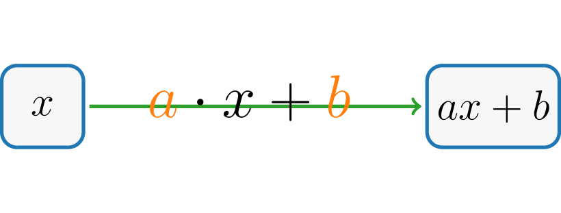
(a)

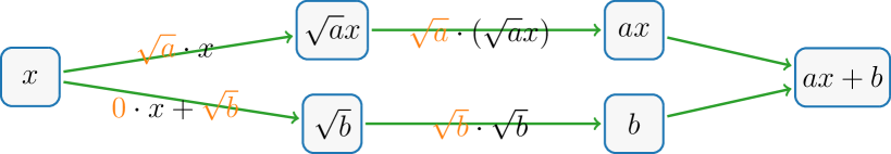
(b)

Figure 2: Illustrations of the magnitude reduction of parameters for a sub-network. The parameters are marked in orange. Without loss of generality, $a\gg 1$ and $b\gg 1$. (a) Return $ax+b$ via two large parameters $a$ and $b$. (b) Return $ax+b$ via several small parameters bounded by $\max\{\sqrt{a},\sqrt{b}\}$.

In real-world applications, the parameters of the EUAF network are learned from the samples of the target function, which involves sophisticated numerical optimization. We refer to the learnability of network parameters as the existence of a numerical optimization algorithm that can identify network parameters to achieve a target approximation error. The computability of the EUAF networks does not imply learnability, which involves approximation, optimization, and generalization error analyses. The result in this paper shows that there exist computable EUAF networks achieving an arbitrarily small approximation error. This means the learnability of the best approximation is reduced to achieving small generalization and optimization errors, which depend on the given data, the empirical risk model, and the optimization algorithm. Therefore, whether or not EUAF networks would be useful in real-world applications also depends on optimization and generalization, which is out of the scope of this paper. The optimization and generalization error analyses of practical deep neural networks including EUAF networks is a challenging problem. To the best of our knowledge, there is no complete error analysis to address the learnability of neural networks with nonlinear activation functions.

The rest of this paper is organized as follows. In Section 2, we first summarize notations used in this paper and then discuss the ideas of proving Theorem 1. Section 3 focuses on numerical experimentation of EUAF, which acts as a proof of concept to explore the numerical properties of EUAF. Next, several UAFs with better properties are proposed in Section 4. After that, we use several sections to present the complete proofs of Theorems 1 and 4. In Section 5, by assuming Theorem 6 is true, we give the detailed proofs of Theorems 1 and 4. Theorem 6 is proved in Section 6 based on Proposition 7, the proof of which can be found in Section 7. Finally, Section 8 concludes this paper with a short discussion.

2 Notations and Proof Ideas

In this section, we first summarize notations used in this paper and then discuss the ideas of proving Theorem 1.

2.1 Notations

Let us summarize all basic notations used in this paper as follows.

• Let $\mathbb{R}$, $\mathbb{Q}$, and $\mathbb{Z}$ denote the set of real numbers, rational numbers, and integers, respectively.

• Let $\mathbb{N}$ and $\mathbb{N}^{+}$ denote the set of natural numbers and positive natural numbers, respectively. That is, $\mathbb{N}^{+}=\{1,2,3,{\cdots}\}$ and $\mathbb{N}=\mathbb{N}^{+}\bigcup\{0\}$.

• For any $x\in\mathbb{R}$, let $\lfloor x\rfloor:=\max\{n:n\leq x,\ n\in\mathbb{Z}\}$ and $\lceil x\rceil:=\min\{n:n\geq x,\ n\in\mathbb{Z}\}$.

• Let ${\mathds{1}}_{S}$ be the indicator (characteristic) function of a set $S$, i.e., ${\mathds{1}}_{S}$ is equal to $1$ on $S$ and $0$ outside $S$.

• The set difference of two sets $A$ and $B$ is denoted by $A\backslash B:=\{x:x\in A,\ x\notin B\}$.

• Matrices are denoted by bold uppercase letters. For instance, $\bm{A}\in\mathbb{R}^{m\times n}$ is a real matrix of size $m\times n$, and $\bm{A}^{T}$ denotes the transpose of $\bm{A}$. Vectors are denoted as bold lowercase letters. For example, $\bm{v}=[v_{1},v_{2},{\cdots},v_{d}]^{T}=\scalebox{0.66}{$\left[\begin{array}[]{c}v_{1}\\ v_{2}\\ \vdots\\ v_{d}\end{array}\right]$}\in\mathbb{R}^{d}$ is a column vector. Besides, “$[$” and “$]$” are used to partition matrices (vectors) into blocks, e.g., $\bm{A}=\left[\begin{smallmatrix}\bm{A}_{11}&\bm{A}_{12}\\ \bm{A}_{21}&\bm{A}_{22}\end{smallmatrix}\right]$.

• For any $p\in[1,\infty)$, the $p$-norm (or $\ell^{p}$-norm) of a vector ${\bm{x}}=[x_{1},x_{2},{\cdots},x_{d}]^{T}\in\mathbb{R}^{d}$ is defined by

  $$\|{\bm{x}}\|_{p}=\|{\bm{x}}\|_{\ell^{p}}\coloneqq\big{(}|x_{1}|^{p}+|x_{2}|^{p}+{\cdots}+|x_{d}|^{p}\big{)}^{1/p}.$$

  In the case $p=\infty$,

  $$\|{\bm{x}}\|_{\infty}=\|{\bm{x}}\|_{\ell^{\infty}}\coloneqq\max\big{\{}|x_{i}|:i=1,2,{\cdots},d\big{\}}.$$

• For any $a_{1},a_{2},{\cdots},a_{J}\in\mathbb{R}$, we say $a_{1},a_{2},{\cdots},a_{J}$ are rationally independent if they are linearly independent over the rational numbers $\mathbb{Q}$. That is, if there exist $\lambda_{1},\lambda_{2},{\cdots},\lambda_{J}\in\mathbb{Q}$ such that $\sum_{j=1}^{J}\lambda_{j}\cdot a_{j}=0$, then $\lambda_{1}=\lambda_{2}={\cdots}=\lambda_{J}=0$. For a simple example, $1$, $\sqrt{2}$, and $\sqrt{3}$ are rationally independent.

• An algebraic number is any complex number (including real numbers) that is a root of a polynomial equation with rational coefficients, i.e., $\alpha$ is an algebraic number if and only if there exist $\lambda_{0},\lambda_{1},{\cdots},\lambda_{J}\in\mathbb{Q}$ with $\sum_{j=0}^{J}\lambda_{j}\alpha^{j}=0$. Denote the set of all algebraic numbers by $\mathbb{A}$. We say a complex number is transcendental if it is not in $\mathbb{A}$. The set $\mathbb{A}$ is countable, and, therefore, almost all numbers are transcendental. The best known transcendental numbers are $\pi$ (the ratio of a circle’s circumference to its diameter) and $e$ (the natural logarithmic base).

• The expression “a network (architecture) with width $N$ and depth $L$” means

  • The number of neurons in each hidden layer of this network (architecture) is no more than $N$.

  • The number of hidden layers of this network (architecture) is no more than $L$.

2.2 Key Ideas of Proving Theorem 1

The proof of Theorem 1 has two main steps: 1) prove the one-dimensional case; 2) reduce the $d$-dimensional approximation to the one-dimensional case via KST (Kolmogorov, 1957). In fact, in the case of $d=1$, the size of the network in Theorem 1 can be further reduced as shown in Theorem 6 below. Theorem 6 is actually an enhanced version of Theorem 1 and hence implies Theorem 1 in the case $d=1$.

Theorem 6.

Let $f\in C([a,b])$ be a continuous function. Then, for an arbitrary $\varepsilon>0$, there exists a function $\phi$ generated by an EUAF network with width $36$ and depth $5$ such that

$$|\phi(x)-f(x)|<\varepsilon\quad\textnormal{for any $x\in[a,b]\subseteq\mathbb{R}$.}$$

The detailed proof of Theorem 6 can be found in Section 6. The main ideas of proving Theorem 6 are developed from some ideas of our early works (Shen et al., 2021a, b). Roughly speaking, we eventually convert a function approximation problem in an interval (e.g., $[0,1)$) to a point-fitting problem via the composition architecture of neural networks in the following three main steps.

• Divide $[0,1)$ into small intervals ${\mathcal{I}}_{k}=[\tfrac{k-1}{K},\tfrac{k}{K})$ with a left endpoint $x_{k}$ for $k\in\{1,2,{\cdots},K\}$, where $K$ is an integer determined by the given error and the target function $f$.

• Construct a sub-network to generate a function $\phi_{1}$ mapping the whole interval ${\mathcal{I}}_{k}$ to $k$ for each $k$. The floor function $\lfloor\cdot\rfloor$ is a good choice to implement this step. Precisely, we can define $\phi_{1}(x)=\lfloor Kx\rfloor$. The floor function is not continuous and has zero-derivative almost everywhere. As we shall see later, $\sigma_{1}$ (or $\sigma$) can be a continuous alternative to implement this step, but the construction is more complicated.

• The final step is to design another sub-network to generate a function $\phi_{2}$ mapping $k$ approximately to $f(x_{k})$ for each $k$. Then $\phi_{2}\circ\phi_{1}(x)=\phi_{2}(k)\approx f(x_{k})\approx f(x)$ for any $x\in{\mathcal{I}}_{k}$ and $k\in\{1,2,{\cdots},K\}$, which implies $\phi_{2}\circ\phi_{1}\approx f$ on $[0,1)$. After the above two steps, we simplify the approximation problem to a point-fitting problem, where $k$ is approximately mapped to $f(k)$. This step is the bottleneck of the construction in our previous papers (Shen et al., 2021a, b). Roughly speaking, the final approximation error is essentially determined by how many points we can fit using a neural network.

For the second step, the capacity to generate step functions with sufficiently many “steps” via a sub-network with a limited number of neurons plays an important role. The reproduced step functions can be considered as a continuous version of the floor function ($\lfloor\cdot\rfloor$) in (Shen et al., 2021a, b), which is a perfect step function with infinite “steps” that improves the approximation power of networks as shown in (Shen et al., 2021a, b). The key ingredient in the third step of the proof of Theorem 6 is essentially a point-fitting problem with arbitrarily many points. This requires the following proposition motivated by the well-known fact that an irrational winding on the torus is dense. See Figure 3 for illustrations of such a fact. Here, we propose a new point-fitting technique that can fit arbitrarily many points within an arbitrary error using fixed-size neural networks.

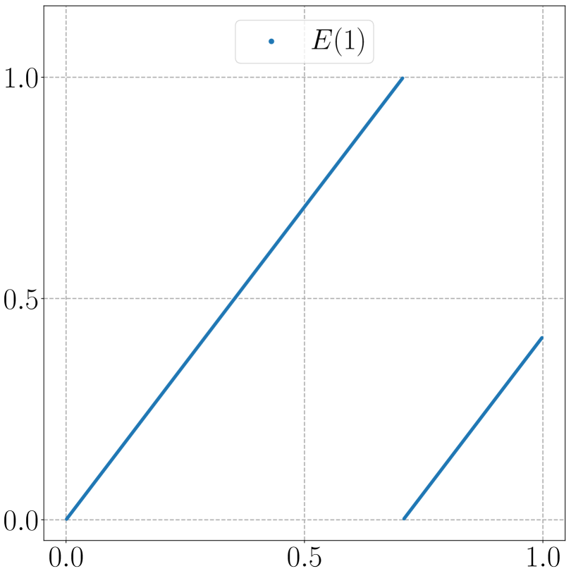
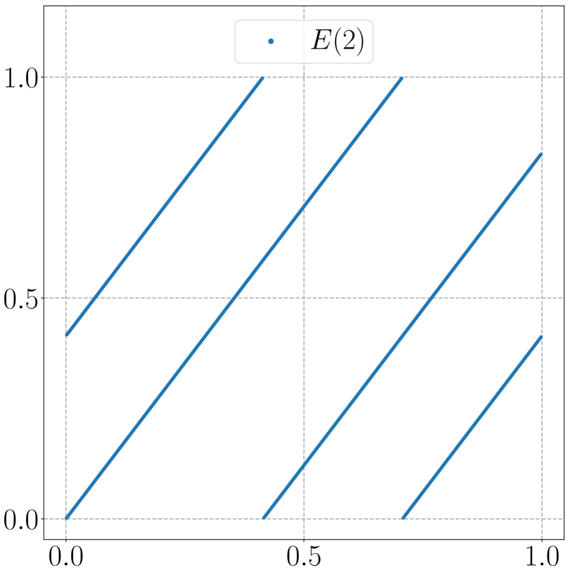
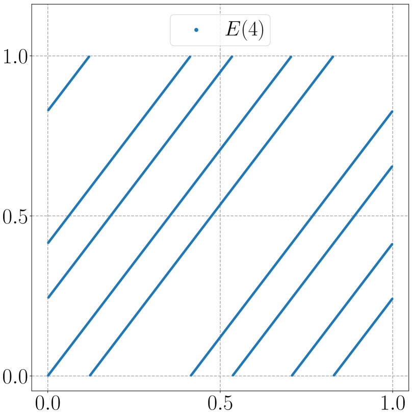
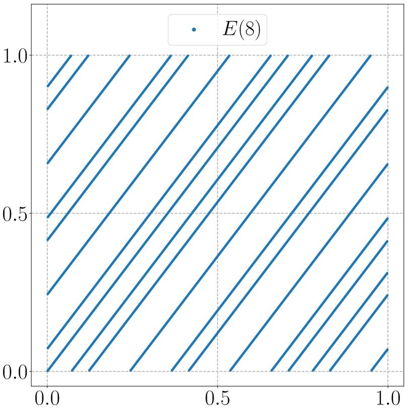
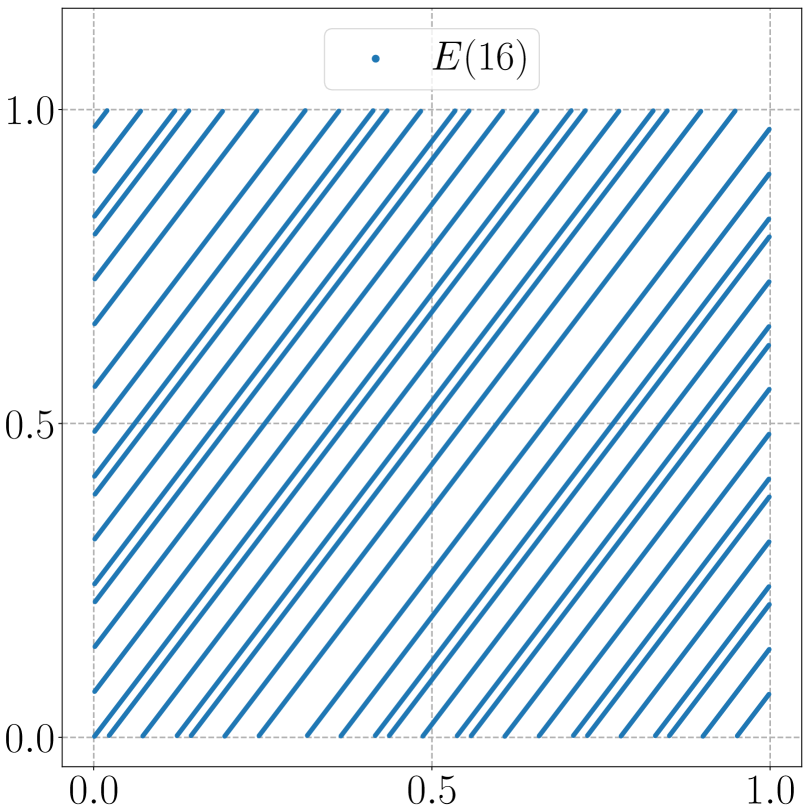
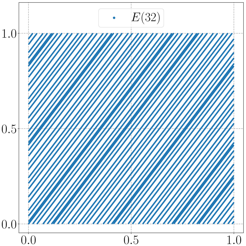
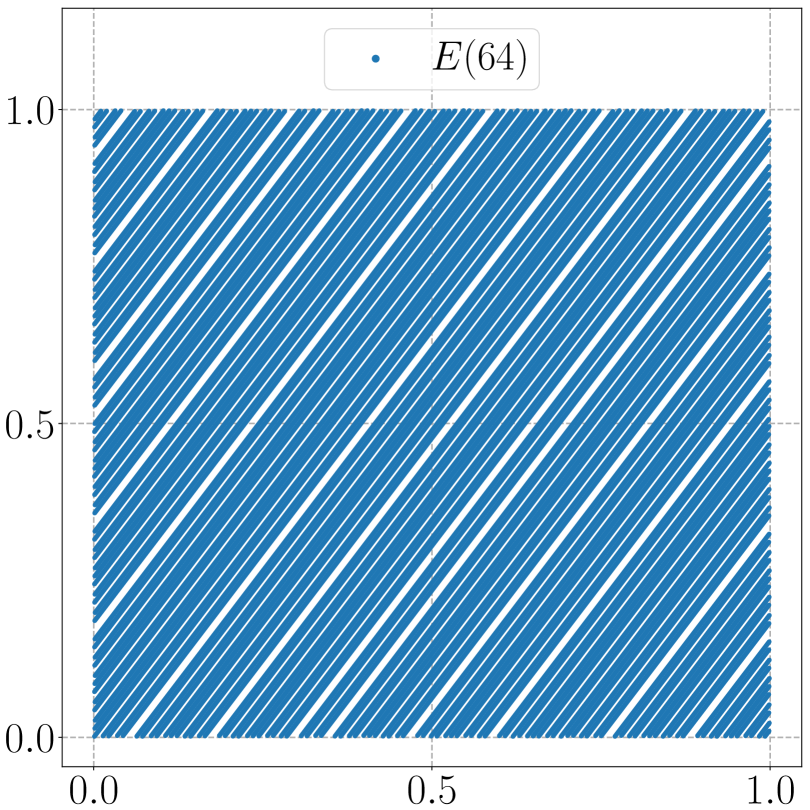
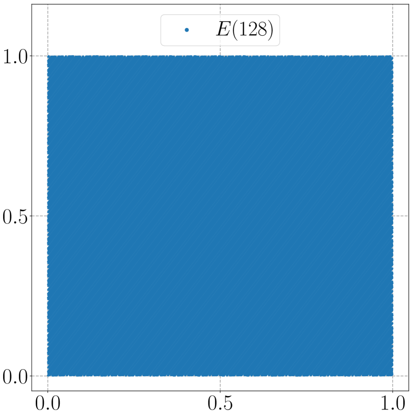
Figure 3: Illustrations of the denseness of $E(\infty)$ in $[0,1]^{2}$, where $E(r)$ is a winding of an “irrational” direction $[1,\sqrt{2}]^{T}$ on $[0,r)$, i.e., $E(r)=\big{\{}[\tau(t),\tau(\sqrt{2}\,t)]^{T}:\,t\in[0,r)\big{\}}$ with $\tau(t)=t-\lfloor t\rfloor$.

Proposition 7.

For any $K\in\mathbb{N}^{+}$, the following point set

$$\Big{\{}\big{[}\sigma_{1}(\tfrac{w}{\pi+1}),\ \sigma_{1}(\tfrac{w}{\pi+2}),\ {\cdots},\ \sigma_{1}(\tfrac{w}{\pi+K})\big{]}^{T}\,:\,w\in\mathbb{R}\Big{\}}\subseteq[0,1]^{K}$$

is dense in $[0,1]^{K}$, where $\pi$ is the ratio of a circle’s circumference to its diameter.

The proof of Proposition 7 can be found in Section 7. To prove the denseness in Proposition 7, we borrow some ideas from transcendental number theory and Diophantine approximations in number theory. The number $\pi$ used in Proposition 7 is transcendental. It can be replaced by any other transcendental number.

Proposition 7 implies that for any given sample points $(k,y_{k})\in\mathbb{R}^{2}$ with $y_{k}\in[0,1]$ for $k=1,2,{\cdots},K$ and any $K\in\mathbb{N}^{+}$, there exists $w_{0}\in\mathbb{R}$ such that the function $x\mapsto\sigma_{1}(\tfrac{w_{0}}{\pi+x})$ can fit the points $(k,y_{k})\in\mathbb{R}^{2}$ for $k=1,2,{\cdots},K$ within an arbitrary pre-specified error $\varepsilon>0$. To put it another way, for any $\varepsilon>0$, there exists $w_{0}\in\mathbb{R}$ such that $|\sigma_{1}(\tfrac{w_{0}}{\pi+k})-y_{k}|<\varepsilon$ for all $k$.

As we shall see later in the proof of Proposition 7, the key point is the periodicity of the outer function $\sigma_{1}$. Of course, the inner function $x\mapsto\tfrac{w_{0}}{\pi+x}$ is also necessary since it helps to adjust sample points for $x=1,2,{\cdots},K$. In fact, the inner function $x\mapsto\tfrac{w_{0}}{\pi+x}$ can be regarded as a variant of $\sigma_{2}$ via scaling and shifting. The periodicity has been explored to improve neural network approximation in the literature, e.g. the sine function in (Yarotsky and Zhevnerchuk, 2020) is periodic and the floor function ($\lfloor\cdot\rfloor$) in (Shen et al., 2021a, b) is implicitly periodic because $x-\lfloor x\rfloor$ is periodic. We remark that a similar result holds if we replace $\sigma_{1}$ by a non-trivial periodic function and replace the sample locations $x=1,2,{\cdots},K$ by distinct rational numbers $r_{1},r_{2},{\cdots},r_{K}\in\mathbb{Q}$. See Section 7 for a further discussion.

Theorem 6 essentially proves Theorem 1 for the univariate case. To prove the general case, we need the Kolmogorov superposition theorem (KST) (Kolmogorov, 1957) given below to reduce a multivariate problem to a one-dimensional case.

Theorem 8 (KST).

There exist continuous functions $h_{i,j}\in C([0,1])$ for $i=0,1,{\cdots},2d$ and $j=1,2,{\cdots},d$ such that any continuous function $f\in C([0,1]^{d})$ can be represented as

$$f({\bm{x}})=\sum_{i=0}^{2d}g_{i}\Big{(}\sum_{j=1}^{d}h_{i,j}(x_{j})\Big{)}\quad\textnormal{for any ${\bm{x}}=[x_{1},x_{2},{\cdots},x_{d}]^{T}\in[0,1]^{d}$,}$$

where $g_{i}:\mathbb{R}\to\mathbb{R}$ is a continuous function for each $i\in\{0,1,{\cdots},2d\}$.

KST is often used to reduce a multidimensional problem to a one-dimensional one. In fact, the compositional representation in KST can be regarded as a special neural network with (complicated) activation functions depending on the target function, which makes KST useless in practical computation. To avoid this dependency, an activation function was designed in (Maiorov and Pinkus, 1999) to construct neural network representations with ${\mathcal{O}}(d)$ neurons that can approximate functions in $C([-1,1]^{d})$ within an arbitrary error. Let us briefly summarize the main ideas in (Maiorov and Pinkus, 1999): 1) Identify a dense and countable subset $\{u_{k}\}_{k=1}^{\infty}$ of $C([-1,1])$, e.g., polynomials with rational coefficients. 2) Construct an activation function $\varrho$ to encode all $u_{k}(x)$ for $x\in[-1,1]$. In fact, for each $k$, $u_{k}|_{[-1,1]}$ is “stored” in $\varrho$ on $[4k,4k+2]$, and the values of $\varrho$ on $[4k+2,4k+4]$ are properly assigned to make $\varrho$ a smooth and monotonically increasing function. That is, let $\varrho(x+4k+1)=a_{k}+b_{k}x+c_{k}u_{k}(x)$ for any $x\in[-1,1]$ with carefully chosen constants $a_{k}$, $b_{k}$, and $c_{k}\neq 0$ such that $\varrho(x)$ can be a sigmoidal function. 3) For any $g\in C([-1,1])$, there exists a one-hidden-layer $\varrho$-activated network with width $3$ approximating $g$ within an arbitrary error $\delta>0$, i.e., there exists $k$ such that $g(x)\mathop{\approx}\limits^{\delta}u_{k}(x)=\tfrac{\varrho(x+4k+1)-a_{k}-b_{k}x}{c_{k}}$ for any $x\in[-1,1]$. 4) Replace the inner and outer functions in KST with these one-hidden-layer networks to achieve a two-hidden-layer $\varrho$-activated network with width ${\mathcal{O}}(d)$ to approximate $f\in C([-1,1]^{d})$ within an arbitrary error $\varepsilon>0$. As we can see, the key point of the construction in (Maiorov and Pinkus, 1999) is to encode a dense and countable subset of the target function space in an activation function.

Note that both (Maiorov and Pinkus, 1999) and this paper use KST to reduce dimension. However, the activation function of (Maiorov and Pinkus, 1999) is complicated without any closed form and there is no efficient numerical algorithm to evaluate it. After encoding a dense subset of continuous function into a single but complicated activation function, one only needs to construct affine linear transformations to select appropriate functions of this dense subset from this complicated activation function to construct approximation. Hence, such a complicated activation function simplifies the proof of the denseness, since the denseness is encoded in the activation function. As a contrast, we design a simple activation function with efficient numerical implementation (see Figure 1 for an illustration) achieving the universal approximation property with fixed-size networks, because simple and implementable activation functions are a basic requirement for a neural network to be used in applications. However, the proof of the denseness of a neural network generated by such a simple activation function becomes difficult. A sophisticated analysis will be developed in the rest of this paper to overcome the difficulties.

3 Experimentation

In this section, we will conduct two simple experiments as a proof of concept to explore the numerical performances of the EUAF activation function. Let us first discuss the numerical implementation of EUAF in PyTorch. To enable the automatic differentiation feature for EUAF, we need to implement EUAF based on PyTorch built-in functions. With the following four built-in functions $\textnormal{abs}(x)=|x|$, $\textnormal{floor}(x)=\lfloor x\rfloor,$

$$\textnormal{softsign}(x)=\frac{x}{|x|+1},\quad\textnormal{and}\quad\textnormal{sign}(x)=\begin{cases}1&\textnormal{if}\ x>0,\\ 0&\textnormal{if}\ x=0,\\ -1&\textnormal{if}\ x<0,\\ \end{cases}$$

we can represent EUAF as

$$\begin{split}\textnormal{EUAF}(x)&=\begin{cases}\textnormal{softsign}(x)&\textnormal{if}\ x<0,\\ \big{|}x-2\lfloor\tfrac{x+1}{2}\rfloor\big{|}&\textnormal{if}\ x\geq 0\end{cases}\\ &=\textnormal{softsign}(x)\cdot\frac{1-\textnormal{sign}(x)}{2}+\Big{|}x-2\big{\lfloor}\frac{x+1}{2}\big{\rfloor}\Big{|}\cdot\frac{1+\textnormal{sign}(x)}{2}\\ &=\textnormal{softsign}(x)\cdot\frac{1-\textnormal{sign}(x)}{2}+\textnormal{abs}\Big{(}x-2\cdot\textnormal{floor}\big{(}\frac{x+1}{2}\big{)}\Big{)}\cdot\frac{1+\textnormal{sign}(x)}{2}.\\ \end{split}$$

Thus, it is numerically cheap to compute EUAF and its subgradient. We believe the EUAF activation function can achieve good results in some real-world applications if proper optimization algorithms are developed for EUAF. In this paper, we only conduct two simple experiments: a function approximation experiment in Section 3.1 and a classification experiment in Section 3.2.

Next, let us briefly discuss when our EUAF activation function would outperform the practically used ones (e.g., ReLU, Sigmoid, and Softsign), which is based on full error analysis in Section 1.3. In our discussion, we take the ReLU activation function as an example and suppose the optimization error is well-controlled. Clearly, replacing ReLU by EUAF can reduce the approximation error, but would result in a large generalization error. Thus, we would expect that EUAF achieves better results than ReLU if the approximation error is larger than the generalization error. That means EUAF would outperform ReLU in the following two cases.

• The approximation error is pretty large (e.g., the target function is sufficiently complicated).

• The generalization error is well-controlled (e.g., there are sufficiently many samples).

If a given problem does not belong to these two cases, one may consider replacing only a small number of ReLUs by EUAFs. In the function approximation experiment in Section 3.1, we first choose a complicated target function and then generate sufficiently many samples to reduce the generalization error. In the classification experiment in Section 3.2, we control the generalization error via three common methods: keeping network parameters small via L2 regularization, dropout (Hinton et al., 2012; Srivastava et al., 2014), and batch normalization (Ioffe and Szegedy, 2015).

3.1 Function Approximation

We will design fully connected neural network (FCNN) architectures activated by ReLU or EUAF to solve a function approximation problem. To better compare the approximation power of ReLU and EUAF activation functions, we choose a complicated (oscillatory) function $f$ as the target function, where $f$ is defined as

$$f(x_{1},x_{2})\coloneqq 0.6\sin(8x_{1})+0.4\sin(16x_{2})\quad\textnormal{ for any $(x_{1},x_{2})\in[0,1]^{2}$.}$$

To compare the numerical performances of ReLU and EUAF activation functions, we design two FCNN architectures with different activation functions. Both of them have $4$ hidden layers and each hidden layer has $80$ neurons. For simplicity, we denote them as FCNN1 and FCNN2. See illustrations of them in Figure 4. FCNN1 is a standard fully connected ReLU network and FCNN2 can be regarded as a variant of FCNN1 by replacing ReLU by EUAF.

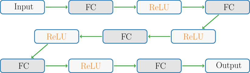
(a) FCNN1.

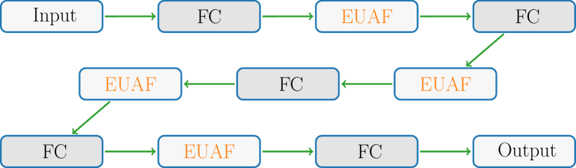
(b) FCNN2.

Figure 4: Illustrations of FCNN1 and FCNN2. FC represents a fully connected layer.

Before presenting the numerical results, let us present the hyper-parameters for training FCNN1 and FCNN2. We randomly choose $10^{6}$ training samples and $10^{5}$ test samples in $[0,1]^{2}$. The number of epochs and the batch size are set to $500$ and $256$, respectively. We adopt RAdam (Liu et al., 2020) as the optimization method and the learning rate is $0.002\times 0.9^{i-1}$ in epochs $5(i-1)+1$ to $5i$ for $i=1,2,{\cdots},100$. Several loss functions are used to estimate the training and test losses, including the mean squared error (MSE), the mean absolute error (MAE), and the maximum (MAX) loss functions. To illustrate MSE, MAE and MAX losses, we denote $\phi$ as the network-generated function and ${\bm{x}}_{1},{\cdots},{\bm{x}}_{m}$ as the test samples ($m=10^{5}$ in our setting). Then, the MSE loss is given by $\tfrac{1}{m}\sum_{i=1}^{m}\big{(}\phi(x_{i})-f(x_{i})\big{)}^{2},$ the MAE loss is given by $\tfrac{1}{m}\sum_{i=1}^{m}\big{|}\phi(x_{i})-f(x_{i})\big{|},$ and the MAX loss is given by $\max\big{\{}|\phi(x_{i})-f(x_{i})|:i=1,2,{\cdots},m\big{\}}.$ The MSE loss is used in our training process. In the settings above, we repeat the experiment $12$ times and discard 2 top-performing and 2 bottom-performing trials by using the average of test losses (MSE) in the last 100 epochs as the performance criterion. For each epoch, we adopt the average of training (test) losses in the rest $8$ trials as the target training (test) loss.

Next, let us present the experiment results to compare the numerical performances of ReLU and EUAF activation functions. Training and test losses (MSE) over epochs for FCNN1 and FCNN2 are summarized in Figure 5.

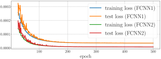
Figure 5: Training and test losses (MSE) in epochs 25-500 for FCNN1 and FCNN2.

In Table 1, we present a comparison of FCNN1 and FCNN2 for the average of the test losses in the last 100 epochs measured in several loss functions. As we can see from Figure 5 and Table 1, FCNN2 performs better than FCNN1. That means replacing ReLU by EUAF would improve experiment results.

	activation function	test loss
		MSE	MAE	MAX
FCNN1	ReLU	$3.53\times 10^{-5}$	$4.57\times 10^{-3}$	$3.69\times 10^{-2}$
FCNN2	EUAF	$7.56\times 10^{-6}$	$2.13\times 10^{-3}$	$1.48\times 10^{-2}$

Table 1: Test loss comparison.

3.2 Classification

The goal of a classification problem with $J\in\mathbb{N}^{+}$ classes is to identify a classification function $f$ defined by

$$f({\bm{x}})=j\quad\textnormal{for any ${\bm{x}}\in E_{j}$ and $j=0,1,{\cdots},J-1$,}$$

where $E_{0},E_{1},{\cdots},E_{J-1}$ are pairwise disjoint bounded closed subsets of $\mathbb{R}^{d}$ and all samples with a label $j$ are contained in $E_{j}$ for each $j$. Such a classification function $f$ can be continuously extended to $\mathbb{R}^{d}$, which means a classification problem can also be regarded as a continuous function approximation problem. We take the case $J=2$ as an example to illustrate the extension. The multiclass case is similar. By defining

$$\textnormal{dist}({\bm{x}},E_{i})\coloneqq\inf_{{\bm{y}}\in E_{i}}\|{\bm{x}}-{\bm{y}}\|_{2}\quad\textnormal{for any ${\bm{x}}\in\mathbb{R}^{d}$ and $i=0,1$,}$$

we have $\textnormal{dist}({\bm{x}},E_{0})+\textnormal{dist}({\bm{x}},E_{1})>0$ for any ${\bm{x}}\in\mathbb{R}^{d}$. Thus, we can define

$$\widetilde{f}({\bm{x}})\coloneqq\frac{\textnormal{dist}({\bm{x}},E_{0})}{\textnormal{dist}({\bm{x}},E_{0})+\textnormal{dist}({\bm{x}},E_{1})}\quad\textnormal{for any ${\bm{x}}\in\mathbb{R}^{d}$}.$$

It is easy to verify that $\widetilde{f}$ is continuous on $\mathbb{R}^{d}$ and

$$\widetilde{f}({\bm{x}})=\begin{cases}0&\textnormal{if}\ {\bm{x}}\in E_{0},\\ 1&\textnormal{if}\ {\bm{x}}\in E_{1}\end{cases}=f({\bm{x}})\quad\textnormal{ for any ${\bm{x}}\in E_{0}\bigcup E_{1}$.}$$

That means $\widetilde{f}$ is a continuous extension of $f$. That means we can apply our theory to classification problems.

We will design convolutional neural network (CNN) architectures activated by ReLU or EUAF to solve a classification problem corresponding to a standard benchmark data set Fashion-MNIST (Xiao et al., 2017). This data set consists of a training set of 60000 samples and a test set of 10000 samples. Each sample is a $28\times 28$ grayscale image, associated with a label from 10 classes. To compare the numerical performances of ReLU and EUAF activation functions, we design two small CNN architectures with different activation functions. Both of them have two convolutional layers and two fully connected layers. For simplicity, we denote them as CNN1 and CNN2. See illustrations of them in Figure 6. We present more details of CNN1 and CNN2 in Table 2.

(a) CNN1.

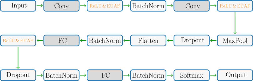
(b) CNN2.

Figure 6: Illustrations of CNN1 and CNN2. Conv and FC represent convolutional and fully connected layers, respectively.

layers	activation function		output size of each layer	dropout	batch normalization
	CNN1	CNN2
input $\in\mathbb{R}^{28\times 28}$			$28\times 28$
Conv-1: $1\times(3\times 3),\,24$	ReLU	$\begin{array}[]{cc}\textnormal{EUAF},\hskip 6.0pt1\times(26\times 26)\\ \textnormal{ReLU},\hskip 6.0pt23\times(26\times 26)\end{array}$	$24\times(26\times 26)$		yes
Conv-2: $24\times(3\times 3),\,24$	ReLU	$\begin{array}[]{cc}\textnormal{EUAF},\hskip 6.0pt1\times(24\times 24)\\ \textnormal{ReLU},\hskip 6.0pt23\times(24\times 24)\end{array}$	$3456$ (MaxPool & Flatten)	$0.25$	yes
FC-1: $3456,\,48$	ReLU	$\begin{array}[]{cc}\textnormal{EUAF},\hskip 6.0pt1\\ \textnormal{ReLU},\hskip 6.0pt47\end{array}$	$48$	$0.5$	yes
FC-2: $48,\,10$			$10$ (Softmax)		yes
output $\in\mathbb{R}^{10}$

Table 2: Details of CNN1 and CNN2.

CNN1 is activated by ReLU, while CNN2 is activated by ReLU and EUAF. In CNN2, only one channel (neuron) of a convolutional (fully connected) hidden layer is activated by EUAF. CNN2 can be regarded as a variant of CNN1 by replacing a small number of ReLUs by EUAFs. This follows a natural question: Why do we not make all (or most) neurons (channels) of CNN2 activated by EUAF? We use only a few EUAFs in CNN2 for two reasons listed below.

• Since the number of available training samples is limited, using too many EUAF activation functions would lead to a large generalization error.

• The key difference of EUAF to the practical used activation functions (e.g., ReLU, Sigmoid, and Softsign) is the periodic part on $[0,\infty)$. As we shall see later in the proof of our main theorem, only a small number of neurons in the constructed network require the periodic property. Thus, we would expect that neural networks activated by the practical used activation functions and a few EUAFs are super expressive.

Next, let us discuss why we choose relatively small network architectures. Since the Fashion-MNIST classification problem is simple, the expressive power of a relatively large ReLU CNN architecture is enough. That means there is no need to introduce EUAF if the network architecture is relatively large. We believe EUAF would be useful for complicated classification problems.

We remark that we use CNNs to approximate an equivalent variant ${\widehat{\bm{f}}}$ of the original classification function $f$ mentioned previously, where ${\widehat{\bm{f}}}$ is given by

$${\widehat{\bm{f}}}({\bm{x}})={\bm{e}}_{j}\quad\textnormal{for any ${\bm{x}}\in E_{j}$ and $j=0,1,{\cdots},J-1$,}$$

where $\{{\bm{e}}_{1},{\bm{e}}_{2},{\cdots},{\bm{e}}_{J}\}$ is the standard basis of $\mathbb{R}^{J}$, i.e., ${\bm{e}}_{j}\in\mathbb{R}^{J}$ denotes the vector with a $1$ in the $j$-th coordinate and $0$’s elsewhere.

Before presenting the numerical results, let us present the hyper-parameters for training two CNN architectures above. We use the cross-entropy loss function to evaluate the loss. The number of epochs and the batch size are set to $500$ and $128$, respectively. We adopt RAdam (Liu et al., 2020) as the optimization method. The weight decay of the optimizer is $0.0001$ and the learning rate is $0.002\times 0.9^{i-1}$ in epochs $5(i-1)+1$ to $5i$ for $i=1,2,{\cdots},100$. All training (test) samples in the Fashion-MNIST data set are standardized in our experiment, i.e., we rescale all training (test) samples to have a mean of $0$ and a standard deviation of $1$. In the settings above, we repeat the experiment $48$ times and discard $8$ top-performing and $8$ bottom-performing trials by using the average of test accuracy in the last 100 epochs as the performance criterion. For each epoch, we adopt the average of test accuracies in the rest $32$ trials as the target test accuracy.

Let us present the experiment results to compare the numerical performances of CNN1 and CNN2. The test accuracy comparison of CNN1 and CNN2 is summarized in Table 3.

	activation function	largest accuracy	average of largest 100 accuracies	average accuracy in last 100 epochs
CNN1	ReLU	0.933066	0.932852	0.932698
CNN2	ReLU and EUAF	0.933922	0.933685	0.933508

Table 3: Test accuracy comparison.

For each of CNN1 and CNN2, we present the largest test accuracy, the average of largest $100$ test accuracies over epochs, and the average of test accuracies in the last 100 epochs. For an intuitive comparison, we also provide illustrations of the test accuracy over epochs for CNN1 and CNN2 in Figure 7. As we can see from Table 3 and Figure 7, CNN2 performs better than CNN1. That means replacing a small number of ReLUs by EUAFs would improve the experiment results.

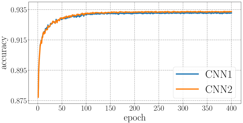
(a) Epochs 1-400.

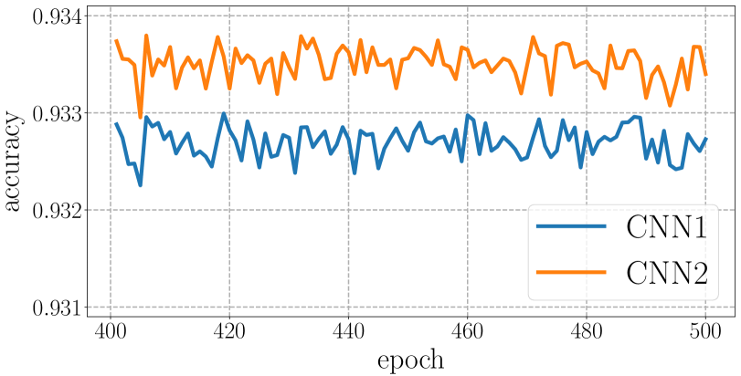
(b) Epochs 401-500.

Figure 7: Test accuracy over epochs.

4 Other Examples of UAFs

This section aims at designing new UAFs with additional properties such as smooth or sigmoidal functions. As discussed in the introduction and shown in the proof of our main theorem, the construction of UAFs mainly relies on three properties: high nonlinearity, periodicity, and the capacity to reproduce step functions. The EUAF $\sigma$ defined in Equation (1) is a simple and typical example of UAFs satisfying these three properties. Indeed, having these properties plays an important role in our proof and is a necessary but not sufficient condition for designing a UAF. In other words, these properties are important, but cannot guarantee the successful construction of UAFs.

Here, we present another idea to design new UAFs, which mainly relies on the following observation: If a UAF $\varrho$ can be approximated by a fixed-size network activated by a new activation function ${\widetilde{\varrho}}$ within an arbitrary error on any bounded interval, then ${\widetilde{\varrho}}$ is also a UAF. Such an observation is a direct result of the lemma below.

Lemma 9.

Let $\varrho,{\widetilde{\varrho}}:\mathbb{R}\to\mathbb{R}$ be two functions with $\varrho\in C(\mathbb{R})$. For an arbitrary given function $f\in[a,b]^{d}\to\mathbb{R}$ and any $\varepsilon>0$, suppose that the following two conditions hold:

• There exists a function $\phi_{\varrho}$ realized by a $\varrho$-activated network with width $N$ and depth $L$ such that

  $$|\phi_{\varrho}({\bm{x}})-f({\bm{x}})|<\varepsilon/2\quad\textnormal{for any ${\bm{x}}\in[a,b]^{d}$.}$$

• For any $M>0$ and each $\delta\in(0,1)$, there exists a function $\varrho_{\delta}$ realized by a ${\widetilde{\varrho}}$-activated network with width ${\widetilde{N}}$ and depth ${\widetilde{L}}$ such that

  $$\varrho_{\delta}(t)\rightrightarrows\varrho(t)\quad\textnormal{as}\quad\delta\to 0^{+}\quad\textnormal{for any $t\in[-M,M]$,}$$

  where $\rightrightarrows$ denotes the uniform convergence.

Then, there exists a function $\phi=\phi_{{\widetilde{\varrho}}}$ generated by a ${\widetilde{\varrho}}$-activated network with width $N\cdot{\widetilde{N}}$ and depth $L\cdot{\widetilde{L}}$ such that

$$|\phi({\bm{x}})-f({\bm{x}})|<\varepsilon\quad\textnormal{for any ${\bm{x}}\in[a,b]^{d}$.}$$

The proof of Lemma 9 is placed in Section 4.3. Based on Lemma 9, we will propose two UAFs with better mathematical properties. That is, the idea of designing a $C^{s}$ UAF is given in Section 4.1 and a sigmoidal UAF is constructed in detail in Section 4.2.

4.1 Smooth UAF

The smoothness of a function is one of the most desired properties in mathematical modeling and computation. The EUAF $\sigma$ is continuous but not smooth. So we will show how to construct a $C^{s}$ UAF based on an existing one. The key point is the fact that the indefinite integral of a continuous function is continuously differentiable.

Suppose $\varrho$ is a continuous UAF. Define

$${\widetilde{\varrho}}(x)\coloneqq\int_{0}^{x}\varrho(t)\textnormal{d}t\quad\textnormal{ for any $x\in\mathbb{R}$.}$$

For any $M>0$, it holds that

$$\frac{{\widetilde{\varrho}}(x+\delta)-{\widetilde{\varrho}}(x)}{\delta}=\frac{1}{\delta}\int_{x}^{x+\delta}\varrho(t)\textnormal{d}t\rightrightarrows\varrho(x)\quad\textnormal{as}\quad\delta\to 0^{+}\quad\textnormal{for any $x\in[-M,M]$}.$$

This means $\varrho$ can be approximated by a one-hidden-layer ${\widetilde{\varrho}}$-activated network with width $2$ arbitrarily well on any bounded interval. It follows that ${\widetilde{\varrho}}$ is also a UAF. By repeated applications of the above idea, one could easily construct a $C^{s}$ UAF.

In particular, set $\varrho_{0}=\sigma$ and define $\varrho_{1},\varrho_{2},{\cdots},\varrho_{s}$ by induction as follows.

$$\varrho_{i+1}(x)\coloneqq\int_{0}^{x}\varrho_{i}(t)\textnormal{d}t\quad\textnormal{for any $x\in\mathbb{R}$ and $i\in\{0,1,{\cdots},s-1\}$.}$$ (6)

Then $\varrho_{s}$ is a $C^{s}$ UAF as shown in the following theorem.

Theorem 10.

Let $\varrho_{s}\in C^{s}(\mathbb{R})$ be the function defined in Equation (6) for any $s\in\mathbb{N}^{+}$. Then, for any $f\in C([a,b]^{d})$ and any $\varepsilon>0$, there exists a function $\phi$ generated by a $\varrho_{s}$-activated network with width $72sd(2d+1)$ and depth $11$ such that

$$|\phi({\bm{x}})-f({\bm{x}})|<\varepsilon\quad\textnormal{for any ${\bm{x}}\in[a,b]^{d}$.}$$

Proof.

For any $i\in\{0,1,{\cdots},s-1\}$ and any $M>0$, it is easy to verify that

$$\frac{\varrho_{i+1}(x+\delta)-\varrho_{i+1}(x)}{\delta}=\frac{1}{\delta}\int_{x}^{x+\delta}\varrho_{i}(t)\textnormal{d}t\rightrightarrows\varrho_{i}(x)\quad\textnormal{as}\quad\delta\to 0^{+}\quad\textnormal{for any $x\in[-M,M]$}.$$

This means $\varrho_{i}$ can be approximated by a one-hidden-layer $\varrho_{i+1}$-activated network with width $2$ arbitrarily well on any bounded interval. By induction, one could easily prove that $\varrho_{0}=\sigma$ can be approximated by a one-hidden-layer $\varrho_{s}$-activated network with width $2s$ arbitrarily well on any bounded interval. That is, for each $\delta\in(0,1)$, there exists a function $\sigma_{s,\delta}$ realized by a $\varrho_{s}$-activated network with width $2s$ and depth $1$ such that

$$\sigma_{s,\delta}(t)\rightrightarrows\sigma(t)\quad\textnormal{as}\quad\delta\to 0^{+}\quad\textnormal{for any $t\in[-M,M]$.}$$

By Theorem 1, there exists a function $\phi_{\sigma}$ generated by a $\sigma$-activated network with width $36d(2d+1)$ and depth $11$ such that

$$|\phi_{\sigma}({\bm{x}})-f({\bm{x}})|<\varepsilon/2\quad\textnormal{for any ${\bm{x}}\in[a,b]^{d}$.}$$

Then, by Lemma 9, there exists another function $\phi=\phi_{\varrho_{s}}$ realized by a $\varrho_{s}$-activated network with width $2s\times 36d(2d+1)=72sd(2d+1)$ and depth $1\times 11=11$ such that

$$|\phi({\bm{x}})-f({\bm{x}})|<\varepsilon\quad\textnormal{for any ${\bm{x}}\in[a,b]^{d}$.}$$

So we finish the proof. ∎

4.2 Sigmoidal UAF

Many activation functions used in real-world applications are sigmoidal functions. Generally, we say a function $g:\mathbb{R}\to\mathbb{R}$ is sigmoidal (or sigmoid, e.g., see (Han and Moraga, 1995)) if it satisfies the following conditions.

• Bounded: $\lim_{x\to\infty}g(x)=1$ and $\lim_{x\to-\infty}g(x)=-1$ (or $0$).

• Differentiable: $g^{\prime}(x)$ exists and continuous for all $x\in\mathbb{R}$.

• Increasing: $g^{\prime}(x)$ is non-negative for all $x\in\mathbb{R}$.

Our goal is to construct a sigmoidal UAF. To this end, we need to design a new function ${\widetilde{\sigma}}$ based on $\sigma$ such that $\sigma$ can be reproduced/approximated by a ${\widetilde{\sigma}}$-activated network with a fixed size. Making ${\widetilde{\sigma}}$ bounded and increasing is not difficult. The key is to make ${\widetilde{\sigma}}$ continuously differentiable, which can be implemented by the fact that the indefinite integral of a continuous function is continuously differentiable. To be exact, we can define ${\widetilde{\sigma}}$ as follows.

• For $x\in(-\infty,0]$, define ${\widetilde{\sigma}}(x)\coloneqq\sigma(x)=\tfrac{x}{-x+1}$.

• For $x\in(0,\infty)$, define

  $${\widetilde{\sigma}}(x)\coloneqq\int_{0}^{x}\frac{c\sigma(t)+1}{(2t+1)^{2}}\textnormal{d}t,\quad\textnormal{where}\quad c=\frac{1}{2\int_{0}^{\infty}\frac{\sigma(t)}{(2t+1)^{2}}\textnormal{d}t}\approx 2.554.$$

We remark that there are many possible choices for the integrand in the above definition of ${\widetilde{\sigma}}(x)$ for $x\in(0,\infty)$. Here, we just give a simple example. See an illustration of ${\widetilde{\sigma}}$ in Figure 8.

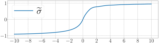
Figure 8: An illustration of ${\widetilde{\sigma}}$ on $[-10,10]$.

Then ${\widetilde{\sigma}}$ is a sigmoidal function as verified below.

• Clearly, $\lim_{x\to-\infty}{\widetilde{\sigma}}(x)=\lim_{x\to-\infty}\tfrac{x}{-x+1}=-1$. Moreover,

  $$\lim_{x\to\infty}{\widetilde{\sigma}}(x)=\int_{0}^{\infty}\frac{c\sigma(t)+1}{(2t+1)^{2}}\textnormal{d}t=\frac{1}{2}+\int_{0}^{\infty}\frac{1}{(2t+1)^{2}}\textnormal{d}t=1.$$

• Obviously, ${\widetilde{\sigma}}$ is continuously differentiable on $(-\infty,0)$ and $(0,\infty)$. Meanwhile, we have ${\widetilde{\sigma}}^{\prime}(0)=1$ and $\lim_{x\to 0}{\widetilde{\sigma}}^{\prime}(x)=1$. Therefore, we have ${\widetilde{\sigma}}\in C^{1}(\mathbb{R})$ as desired.

• For $x\in(-\infty,0)$, ${\widetilde{\sigma}}^{\prime}(x)=\tfrac{1}{(-x+1)^{2}}>0$. For $x=0$, ${\widetilde{\sigma}}^{\prime}(x)=1>0$. For $x\in(0,\infty)$, ${\widetilde{\sigma}}^{\prime}(x)=\tfrac{c\sigma(x)+1}{(2x+1)^{2}}>0$. Therefore, ${\widetilde{\sigma}}^{\prime}(x)>0$ for all $x\in\mathbb{R}$.

Based on Theorem 1 corresponding to $\sigma$, we establish a similar theorem for ${\widetilde{\sigma}}$, Theorem 11 below, showing that fixed-size ${\widetilde{\sigma}}$-activated networks can also approximate continuous functions within an arbitrary error on a hypercube.

Theorem 11.

For any $f\in C([a,b]^{d})$ and any $\varepsilon>0$, there exists a function $\phi$ generated by a ${\widetilde{\sigma}}$-activated network with width $1800d(2d+1)$ and depth $66$ such that

$$|\phi({\bm{x}})-f({\bm{x}})|<\varepsilon\quad\textnormal{for any ${\bm{x}}\in[a,b]^{d}$.}$$

To prove this theorem based on Theorem 1, we only need to show $\sigma$ can be approximated by a fixed-size ${\widetilde{\sigma}}$-activated network within an arbitrary error on any pre-specified interval as presented in the following lemma.

Lemma 12.

For any $\varepsilon>0$ and any $M>0$, there exists a function $\phi$ realized by a ${\widetilde{\sigma}}$-activated network with width $50$ and depth $6$ such that

$$|\phi(x)-\sigma(x)|<\varepsilon\quad\textnormal{for any $x\in[-M,M]$.}$$

The proof of Lemma 12 can be found later. By assuming Lemma 12 is true, we can give the proof of Theorem 11.

Proof of Theorem 11.

By Theorem 1, there exists a function $\phi_{\sigma}$ generated by a $\sigma$-activated network with width $36d(2d+1)$ and depth $11$ such that

$$|\phi_{\sigma}({\bm{x}})-f({\bm{x}})|<\varepsilon/2\quad\textnormal{for any ${\bm{x}}\in[a,b]^{d}$.}$$

By Lemma 12, for any $M>0$ and each $\delta\in(0,1)$, there exists a function $\sigma_{\delta}$ realized by a ${\widetilde{\sigma}}$-activated network with width $50$ and depth $6$ such that

$$\sigma_{\delta}(t)\rightrightarrows\sigma(t)\quad\textnormal{as}\quad\delta\to 0^{+}\quad\textnormal{for any $t\in[-M,M]$.}$$

Then, by Lemma 9, there exists another function $\phi=\phi_{{\widetilde{\sigma}}}$ realized by a ${\widetilde{\sigma}}$-activated network with width $50\times 36d(2d+1)=1800d(2d+1)$ and depth $6\times 11=66$ such that

$$|\phi({\bm{x}})-f({\bm{x}})|<\varepsilon\quad\textnormal{for any ${\bm{x}}\in[a,b]^{d}$.}$$

So we finish the proof. ∎

Finally, let us present the detailed proof of Lemma 12.

Proof of Lemma 12.

Since $1={\widetilde{\sigma}}^{\prime}(0)=\lim_{x\to 0}\tfrac{{\widetilde{\sigma}}(x)}{x}$, it is easy to show: For any ${\mathscr{E}}>0$ and any $R>0$, there exists a sufficiently small $w>0$ such that

$$\big{|}{\widetilde{\sigma}}(wx)/w-x\big{|}<{\mathscr{E}}\quad\textnormal{for any $x\in[-R,R]$.}$$

Thus, we may assume the identity map is allowed to be the activation function in ${\widetilde{\sigma}}$-activated networks. Without loss of generality, we may assume $M\geq 2$ because $\widehat{M}=\max\{2,M\}$ implies $\widehat{M}\geq 2$ and $[-M,M]\subseteq[-\widehat{M},\widehat{M}]$.

For simplicity, we denote ${\widetilde{\mathscr{H}}}(N,L)$ as the (hypothesis) space of functions generated by ${\widetilde{\sigma}}$-activated networks with width $N$ and depth $L$. Then the proof can be roughly divided into three steps as follows.

1. Design $\Gamma\in{\widetilde{\mathscr{H}}}(9,2)$ to reproduce $xy$ on $[-4{\widetilde{M}},4{\widetilde{M}}]^{2}$, where ${\widetilde{M}}=(M+1)^{2}$.

2. Design $\psi_{\delta}\in{\widetilde{\mathscr{H}}}(9,4)$ based on the first step to approximate $\sigma$ well on $[0,M]$.

3. Design $\phi\in{\widetilde{\mathscr{H}}}(50,6)$ based on the previous two steps to approximate $\sigma$ well on $[-M,M]$.

The details of these three steps can be found below.

Step $1\colon$ Design $\Gamma\in{\widetilde{\mathscr{H}}}(9,2)$ to reproduce $xy$ on $[-4{\widetilde{M}},4{\widetilde{M}}]^{2}$.

Observe that

$${\widetilde{\sigma}}(y)+1=\frac{y}{|y|+1}+1=\frac{y}{-y+1}+1=\frac{1}{-y+1}\quad\textnormal{for any $y\leq 0$.}$$

For any $x\in[-4,4]$, we have $-x-4\leq 0$ and $-x-5\leq 0$, implying

$$\begin{split}{\widetilde{\sigma}}(-x-4)-{\widetilde{\sigma}}(-x-5)&=\Big{(}{\widetilde{\sigma}}(-x-4)+1\Big{)}-\Big{(}{\widetilde{\sigma}}(-x-5)+1\Big{)}\\ &=\frac{1}{-(-x-4)+1}-\frac{1}{-(-x-5)+1}\\ &=\frac{1}{x+5}-\frac{1}{x+6}=\frac{1}{(x+5)(x+6)}.\end{split}$$

It follows from $1-\tfrac{90}{(x+5)(x+6)}\leq 0$ for any $x\in[-4,4]$ that

$$\begin{split}{\widetilde{\sigma}}\Big{(}1-\frac{90}{(x+5)(x+6)}\Big{)}+1=\frac{1}{-\big{(}1-\tfrac{90}{(x+5)(x+6)}\big{)}+1}=\frac{x^{2}+11x+30}{90},\end{split}$$

implying

$$\begin{split}x^{2}&=90{\widetilde{\sigma}}\Big{(}1-\frac{90}{(x+5)(x+6)}\Big{)}+90-(11x+30)\\ &=90{\widetilde{\sigma}}\Big{(}1-90\big{(}{\widetilde{\sigma}}(-x-4)-{\widetilde{\sigma}}(-x-5)\big{)}\Big{)}-11x+60\\ &=90{\widetilde{\sigma}}\Big{(}1-90{\widetilde{\sigma}}(-x-4)+90{\widetilde{\sigma}}(-x-5)\Big{)}-11x+60.\end{split}$$

Thus, $x^{2}$ can be realized by a ${\widetilde{\sigma}}$-activated network with width $3$ and depth $2$ on $[-4,4]$. Set ${\widetilde{M}}=(M+1)^{2}$. Then, for any $x,y\in[-4{\widetilde{M}},4{\widetilde{M}}]$, we have $\tfrac{x}{2{\widetilde{M}}},\tfrac{y}{2{\widetilde{M}}},\tfrac{x+y}{2{\widetilde{M}}}\in[-4,4]$. Recall the fact

$$xy=2{\widetilde{M}}^{2}\Big{(}(\tfrac{x+y}{2{\widetilde{M}}})^{2}-(\tfrac{x}{2{\widetilde{M}}})^{2}-(\tfrac{y}{2{\widetilde{M}}})^{2}\Big{)}.$$

Therefore, $xy$ can be realized by a ${\widetilde{\sigma}}$-activated network with width $9$ and depth $2$ for any $x,y\in[-4{\widetilde{M}},4{\widetilde{M}}]$. That is, there exists $\Gamma\in{\widetilde{\mathscr{H}}}(9,2)$ such that $\Gamma(x,y)=xy$ on $[-4{\widetilde{M}},4{\widetilde{M}}]^{2}$.

Step $2\colon$ Design $\psi_{\delta}\in{\widetilde{\mathscr{H}}}(9,4)$ to approximate $\sigma$ well on $[0,M]$.

Recall that $x^{2}$ can be realized by a ${\widetilde{\sigma}}$-activated network with width $3$ and depth $2$ on $[-4,4]$. There exists $\psi_{1}\in{\widetilde{\mathscr{H}}}(3,2)$ such that

$$\psi_{1}(x)=\frac{(2x+1)^{2}}{(2M+1)^{2}}\quad\textnormal{for any $x\in[-M,M]$.}$$

For any small $\delta>0$, we define

$$\psi_{2,\delta}(x)\coloneqq\frac{{\widetilde{\sigma}}(x+\delta)-{\widetilde{\sigma}}(x)}{\delta}\quad\textnormal{for any $x\in\mathbb{R}$.}$$

Then, we have $\psi_{2,\delta}\in{\widetilde{\mathscr{H}}}(2,1)$ and

$$\psi_{2,\delta}(x)\coloneqq\frac{{\widetilde{\sigma}}(x+\delta)-{\widetilde{\sigma}}(x)}{\delta}\rightrightarrows\frac{\textnormal{d}}{\textnormal{d}x}{\widetilde{\sigma}}(x)=\frac{c\sigma(x)+1}{(2x+1)^{2}}\quad\textnormal{as}\quad\delta\to 0^{+}$$

for any $x\in[0,M]$, where $c$ is a constant given by

$$c=\frac{1}{2\int_{0}^{\infty}\frac{\sigma(t)}{(2t+1)^{2}}\textnormal{d}t}\approx 2.554.$$

For any small $\delta>0$, we define

$$\psi_{\delta}(x)\coloneqq\tfrac{(2M+1)^{2}}{c}\Gamma\Big{(}\psi_{1}(x),\psi_{2,\delta}(x)\Big{)}-\tfrac{1}{c}\quad\textnormal{for any $x\in\mathbb{R}.$}$$

Since $\Gamma\in{\widetilde{\mathscr{H}}}(9,2)$, $\psi_{1}\in{\widetilde{\mathscr{H}}}(3,2)$, and $\psi_{2,\delta}\in{\widetilde{\mathscr{H}}}(2,1)$, we have $\psi_{\delta}\in{\widetilde{\mathscr{H}}}(9,4)$.

Clearly, for any $x\in[0,M]$, we have $\psi_{1}(x)=\tfrac{(2x+1)^{2}}{(2M+1)^{2}}\in[0,1]$ and $\psi_{2,\delta}(x)\rightrightarrows\tfrac{c\sigma(x)+1}{(2x+1)^{2}}\in[0,c+1]\subseteq[0,3.6]$, implying $\psi_{1}(x),\psi_{2,\delta}(x)\in[-4,4]\subseteq[-4{\widetilde{M}},4{\widetilde{M}}]$ for any small $\delta>0$. Thus, for any $x\in[0,M]$, as $\delta$ goes to $0^{+}$, we have

$$\begin{split}\psi_{\delta}(x)&=\tfrac{(2M+1)^{2}}{c}\Gamma\Big{(}\psi_{1}(x),\psi_{2,\delta}(x)\Big{)}-\tfrac{1}{c}=\tfrac{(2M+1)^{2}}{c}\cdot\psi_{1}(x)\cdot\psi_{2,\delta}(x)-\tfrac{1}{c}\\ &\rightrightarrows\tfrac{(2M+1)^{2}}{c}\cdot\tfrac{(2x+1)^{2}}{(2M+1)^{2}}\cdot\tfrac{c\sigma(x)+1}{(2x+1)^{2}}-\tfrac{1}{c}=\sigma(x).\end{split}$$

That is, for any $x\in[0,M]$,

$$\psi_{\delta}(x)\rightrightarrows\sigma(x)\quad\textnormal{as}\quad\delta\to 0^{+}.$$

Step $3\colon$ Design $\phi\in{\widetilde{\mathscr{H}}}(50,6)$ to approximate $\sigma$ well on $[-M,M]$.

Note that ${\widetilde{\sigma}}(x)=\sigma(x)$ for all $x\in[-M,0)$ and $\psi_{\delta}(x)$ approximates $\sigma(x)$ well for all $x\in[0,M]$. Then, we have

$$\psi_{\delta}(x)\cdot{\mathds{1}}_{\{x\in[0,M]\}}+{\widetilde{\sigma}}(x)\cdot{\mathds{1}}_{\{x\in[-M,0)\}}$$

approximates $\sigma(x)$ well for all $x\in[-M,M]$. However, it is impossible to approximate ${\mathds{1}}_{\{x\in[0,M]\}}$ well by a ${\widetilde{\sigma}}$-activated network due to the continuity of ${\widetilde{\sigma}}$. To address this gap, we will construct a continuous function $g$ to replace ${\mathds{1}}_{\{x\in[0,M]\}}$ such that

$$\psi_{\delta}(x)\cdot g(x)+{\widetilde{\sigma}}(x)\cdot\big{(}1-g(x)\big{)}$$ (7)

can also approximate $\sigma(x)$ well for all $x\in[-M,M]$.

By the continuity of ${\widetilde{\sigma}}$ and $\sigma$, there exists a small $\eta_{0}\in(0,1)$ such that

$$|{\widetilde{\sigma}}(x)|<\varepsilon/6\quad\textnormal{and }\quad|\sigma(x)|<\varepsilon/6\quad\textnormal{for any $x\in[0,\eta_{0}]$}.$$ (8)

Then we define

$$g(x)\coloneqq\frac{\textnormal{ReLU}(x)-\textnormal{ReLU}(x-\eta_{0})}{\eta_{0}},\quad\textnormal{where}\ \textnormal{ReLU}(x)=\max\{0,x\}\quad\textnormal{for any $x\in\mathbb{R}$}.$$

See Figure 9 for an illustration of $g$.

Figure 9: An illustration of $g$ on $[-10,10]$.

We will construct a ${\widetilde{\sigma}}$-activated network to approximate $g$ well. To this end, we first design a ${\widetilde{\sigma}}$-activated network to approximate the ReLU function well. For any $x\in[-M-1,M+1]$, we have $\tfrac{x}{M+1}+1\in[0,2]\subseteq[0,M]$, implying

$$1-\psi_{\delta}(\tfrac{x}{M+1}+1)\rightrightarrows 1-\sigma(\tfrac{x}{M+1}+1)=|\tfrac{x}{M+1}|\quad\textnormal{as}\quad\delta\to 0^{+},$$

where the last equality comes from $1-\sigma(y)=|y-1|$ for any $y\in[0,2]$. Recall that

$$\textnormal{ReLU}(x)=\tfrac{x}{2}+\tfrac{|x|}{2}=\tfrac{x}{2}+\tfrac{M+1}{2}\cdot|\tfrac{x}{M+1}|$$

for any $x\in[-M-1,M+1]$. For any small $\delta>0$, we define

$${\widetilde{g}}_{\delta}(x)\coloneqq\tfrac{x}{2}+\tfrac{M+1}{2}\Big{(}1-\psi_{\delta}(\tfrac{x}{M+1}+1)\Big{)}\quad\textnormal{for any $x\in\mathbb{R}$}.$$

Then, $\psi_{\delta}\in{\widetilde{\mathscr{H}}}(9,4)$ implies ${\widetilde{g}}_{\delta}\in{\widetilde{\mathscr{H}}}(10,4)$. Moreover, for any $x\in[-M-1,M+1]$,

$${\widetilde{g}}_{\delta}(x)\rightrightarrows\tfrac{x}{2}+\tfrac{M+1}{2}\cdot|\tfrac{x}{M+1}|=\textnormal{ReLU}(x)\quad\textnormal{as}\quad\delta\to 0^{+}.$$

Define

$$g_{\delta}(x)\coloneqq\frac{{\widetilde{g}}_{\delta}(x)-{\widetilde{g}}_{\delta}(x-\eta_{0})}{\eta_{0}}\quad\textnormal{for any $x\in\mathbb{R}$}.$$

Clearly, ${\widetilde{g}}_{\delta}\in{\widetilde{\mathscr{H}}}(10,4)$ implies $g_{\delta}\in{\widetilde{\mathscr{H}}}(20,4)$. For any $x\in[-M,M]$, we have $x,x-\eta_{0}\in[-M-1,M+1]$, implying

$$g_{\delta}(x)=\frac{{\widetilde{g}}_{\delta}(x)-{\widetilde{g}}_{\delta}(x-\eta_{0})}{\eta_{0}}\rightrightarrows\frac{\textnormal{ReLU}(x)-\textnormal{ReLU}(x-\eta_{0})}{\eta_{0}}=g(x)\quad\textnormal{as}\quad\delta\to 0^{+}.$$

Next, motivated by Equation (7), we can define $\phi_{\delta}$ to approximate $\sigma$ well on $[-M,M]$. The definition of $\phi_{\delta}$ is given by

$$\phi_{\delta}(x)\coloneqq\Gamma\Big{(}\psi_{\delta}(x),g_{\delta}(x)\Big{)}+\Gamma\Big{(}{\widetilde{\sigma}}(x),1-g_{\delta}(x)\Big{)}\quad\textnormal{for any $x\in\mathbb{R}$.}$$

Since $\Gamma\in{\widetilde{\mathscr{H}}}(9,2)$, $\psi_{\delta}\in{\widetilde{\mathscr{H}}}(9,4)$, and $g_{\delta},1-g_{\delta}\in{\widetilde{\mathscr{H}}}(20,4)$, we have

$$\phi_{\delta}\in{\widetilde{\mathscr{H}}}(9+20+1+20,4+2)={\widetilde{\mathscr{H}}}(50,6).$$

Clearly, ${\widetilde{\sigma}}(x)$, $g_{\delta}(x)$, and $1-g_{\delta}(x)$ are all in $[-4{\widetilde{M}},4{\widetilde{M}}]$ for any small $\delta>0$ and all $x\in[-M,M]$. We will show $\psi_{\delta}(x)\in[-4{\widetilde{M}},4{\widetilde{M}}]$ for any small $\delta>0$ and all $x\in[-M,M]$ via two cases as follows.

• For any $x\in[0,M]$, $\psi_{\delta}(x)\rightrightarrows\sigma(x)$ implies $\psi_{\delta}(x)\in[-4{\widetilde{M}},4{\widetilde{M}}]$ for any small $\delta>0$.

• For any $x\in[-M,0)$, we have $\psi_{1}(x)=\tfrac{(2x+1)^{2}}{(2M+1)^{2}}\in[0,1]$ and

  $$\psi_{2,\delta}(x)=\tfrac{{\widetilde{\sigma}}(x+\delta)-{\widetilde{\sigma}}(x)}{\delta}\rightrightarrows\tfrac{\textnormal{d}}{\textnormal{d}x}{\widetilde{\sigma}}(x)=\tfrac{1}{(-x+1)^{2}}\quad\textnormal{as}\quad\delta\to 0^{+}.$$

  Thus, for any $x\in[-M,0)$, as $\delta$ goes to $0^{+}$, we get

  $$\begin{split}\psi_{\delta}(x)&=\tfrac{(2M+1)^{2}}{c}\Gamma\Big{(}\psi_{1}(x),\psi_{2,\delta}(x)\Big{)}-\tfrac{1}{c}=\tfrac{(2M+1)^{2}}{c}\cdot\psi_{1}(x)\cdot\psi_{2,\delta}(x)-\tfrac{1}{c}\\ &\rightrightarrows\tfrac{(2M+1)^{2}}{c}\cdot\tfrac{(2x+1)^{2}}{(2M+1)^{2}}\cdot\tfrac{1}{(-x+1)^{2}}-\tfrac{1}{c}=\tfrac{(2x+1)^{2}-1}{c(-x+1)^{2}}.\end{split}$$

  For all $x\in[-M,0)$, we have $c(-x+1)^{2}\geq 1$, implying $\tfrac{(2x+1)^{2}-1}{c(-x+1)^{2}}\geq\tfrac{-1}{c(-x+1)^{2}}\geq-1$ and

  $$\begin{split}\tfrac{(2x+1)^{2}-1}{c(-x+1)^{2}}\leq\tfrac{(2|x|+1)^{2}-1}{c(-x+1)^{2}}\leq(2|x|+1)^{2}-1&=4(|x|+1/2)^{2}-1\\ &\leq 4(M+1)^{2}-1=4{\widetilde{M}}-1.\end{split}$$

  That is, $\tfrac{(2x+1)^{2}-1}{c(-x+1)^{2}}\in[-1,4{\widetilde{M}}-1]$ for all $x\in[-M,0)$, implying $\psi_{\delta}(x)\in[-4{\widetilde{M}},4{\widetilde{M}}]$ for any small $\delta>0$.

Hence, for any $x\in[\eta_{0},M]$, we have $1-g(x)=0$, implying

$$\phi_{\delta}(x)=\psi_{\delta}(x)\cdot g_{\delta}(x)+{\widetilde{\sigma}}(x)\cdot\big{(}1-g_{\delta}(x)\big{)}\rightrightarrows\sigma(x)\cdot g(x)+0=\sigma(x)\quad\textnormal{as}\quad\delta\to 0^{+}.$$

Similarly, for any $x\in[-M,0]$, we have $g(x)=0$, implying

$$\phi_{\delta}(x)=\psi_{\delta}(x)\cdot g_{\delta}(x)+{\widetilde{\sigma}}(x)\cdot\big{(}1-g_{\delta}(x)\big{)}\rightrightarrows 0+{\widetilde{\sigma}}(x)\cdot\big{(}1-g(x)\big{)}=\sigma(x)\quad\textnormal{as}\quad\delta\to 0^{+}.$$

Therefore, there exists a small $\delta_{0}>0$ such that

$$|\phi_{\delta_{0}}(x)-\sigma(x)|<\varepsilon\quad\textnormal{for any $x\in[-M,0]\bigcup[\eta_{0},M]$},$$

$\|g_{\delta_{0}}\|_{L^{\infty}([0,\eta_{0}])}\leq 2$, $\|1-g_{\delta_{0}}\|_{L^{\infty}([0,\eta_{0}])}\leq 2$, and

$$\|\psi_{\delta_{0}}\|_{L^{\infty}([0,\eta_{0}])}\leq\|\sigma\|_{L^{\infty}([0,\eta_{0}])}+\varepsilon/12,$$

where the above inequality comes from the fact $\psi_{\delta}(x)$ uniformly converges to $\sigma(x)$ for any $x\in[0,\eta_{0}]\subseteq[0,M]$.

Clearly, for any $x\in[0,\eta_{0}]$, by Equation (8), we have

$$\begin{split}|\phi_{\delta_{0}}(x)-\sigma(x)|\leq|\phi_{\delta_{0}}(x)|+|\sigma(x)|&<\Big{|}\psi_{\delta_{0}}(x)\cdot g_{\delta_{0}}(x)+{\widetilde{\sigma}}(x)\cdot\big{(}1-g_{\delta_{0}}(x)\big{)}\Big{|}+\varepsilon/6\\ &\leq\big{|}\psi_{\delta_{0}}(x)\big{|}\cdot\big{|}g_{\delta_{0}}(x)\big{|}+\big{|}{\widetilde{\sigma}}(x)\big{|}\cdot\big{|}1-g_{\delta_{0}}(x)\big{|}+\varepsilon/6\\ &\leq\big{(}\|\sigma\|_{L^{\infty}([0,\eta_{0}])}+\frac{\varepsilon}{12}\big{)}\cdot 2+\frac{\varepsilon}{6}\cdot 2+\frac{\varepsilon}{6}\\ &\leq\big{(}\frac{\varepsilon}{6}+\frac{\varepsilon}{12}\big{)}\cdot 2+\frac{\varepsilon}{6}\cdot 2+\frac{\varepsilon}{6}=\varepsilon.\end{split}$$

By setting $\phi=\phi_{\delta_{0}}$, we have $\phi=\phi_{\delta_{0}}\in{\widetilde{\mathscr{H}}}(50,6)$ and

$$|\phi(x)-\sigma(x)|=|\phi_{\delta_{0}}(x)-\sigma(x)|<\varepsilon\quad\textnormal{for any $x\in[-M,M]$}.$$

So we finish the proof. ∎

4.3 Proof of Lemma 9

Let the activation function be applied to a vector elementwisely. Then $\phi_{\varrho}$ can be represented in a form of function compositions as follows:

$$\phi_{\varrho}({\bm{x}})={\bm{\mathcal{L}}}_{L}\circ\varrho\circ{\bm{\mathcal{L}}}_{L-1}\circ\ {\cdots}\ \circ\varrho\circ{\bm{\mathcal{L}}}_{1}\circ\varrho\circ{\bm{\mathcal{L}}}_{0}({\bm{x}})\quad\textnormal{for any ${\bm{x}}\in\mathbb{R}^{d}$},$$

where $N_{0}=d$, $N_{1},N_{2},{\cdots},N_{L}\in\mathbb{N}^{+}$, $N_{L+1}=1$, $\bm{A}_{\ell}\in\mathbb{R}^{N_{\ell+1}\times N_{\ell}}$ and $\bm{b}_{\ell}\in\mathbb{R}^{N_{\ell+1}}$ are the weight matrix and the bias vector in the $\ell$-th affine linear transform ${\bm{\mathcal{L}}}_{\ell}:{\bm{y}}\mapsto\bm{A}_{\ell}{\bm{y}}+{\bm{b}}_{\ell}$ for each $\ell\in\{0,1,{\cdots},L\}$. Define

$$\phi_{\varrho_{\delta}}({\bm{x}})\coloneqq{\bm{\mathcal{L}}}_{L}\circ{\varrho_{\delta}}\circ{\bm{\mathcal{L}}}_{L-1}\circ\ {\cdots}\ \circ{\varrho_{\delta}}\circ{\bm{\mathcal{L}}}_{1}\circ\varrho_{\delta}\circ{\bm{\mathcal{L}}}_{0}({\bm{x}})\quad\textnormal{for any ${\bm{x}}\in\mathbb{R}^{d}$}.$$

Recall that $\varrho_{\delta}$ can be realized by a ${\widetilde{\varrho}}$-activated network with width ${\widetilde{N}}$ and depth ${\widetilde{L}}$. Thus, $\phi_{\varrho_{\delta}}$ can be realized by a ${\widetilde{\varrho}}$-activated network with width $N\cdot{\widetilde{N}}$ and depth $L\cdot{\widetilde{L}}$. We will prove

$$\phi_{\varrho_{\delta}}({\bm{x}})\rightrightarrows\phi_{\varrho}({\bm{x}})\quad\textnormal{as}\quad\delta\to 0^{+}\quad\textnormal{for any ${\bm{x}}\in[a,b]^{d}$}.$$

For any ${\bm{x}}\in\mathbb{R}^{d}$ and each $\ell\in\{1,2,{\cdots},L+1\}$, define

$${\bm{h}}_{\ell}({\bm{x}})\coloneqq{\bm{\mathcal{L}}}_{\ell-1}\circ\varrho\circ{\bm{\mathcal{L}}}_{\ell-2}\circ\ {\cdots}\ \circ\varrho\circ{\bm{\mathcal{L}}}_{1}\circ\varrho\circ{\bm{\mathcal{L}}}_{0}({\bm{x}})$$

and

$${\bm{h}}_{\ell,\delta}({\bm{x}})\coloneqq{\bm{\mathcal{L}}}_{\ell-1}\circ\varrho_{\delta}\circ{\bm{\mathcal{L}}}_{\ell-2}\circ\ {\cdots}\ \circ\varrho_{\delta}\circ{\bm{\mathcal{L}}}_{1}\circ\varrho_{\delta}\circ{\bm{\mathcal{L}}}_{0}({\bm{x}}).$$

Note that ${\bm{h}}_{\ell}$ and ${\bm{h}}_{\ell,\delta}$ are two maps from $\mathbb{R}^{d}$ to $\mathbb{R}^{N_{\ell}}$ for each $\ell$.

We will prove by induction that

$${\bm{h}}_{\ell,\delta}({\bm{x}})\rightrightarrows{\bm{h}}_{\ell}({\bm{x}})\quad\textnormal{as}\quad\delta\to 0^{+}$$ (9)

for any ${\bm{x}}\in[a,b]^{d}$ and each $\ell\in\{1,2,{\cdots},L+1\}$.

First, we consider the case $\ell=1$. Clearly,

$${\bm{h}}_{1,\delta}({\bm{x}})={\bm{\mathcal{L}}}_{0}({\bm{x}})={\bm{h}}_{1}({\bm{x}})\quad\textnormal{as}\quad\delta\to 0^{+}\quad\textnormal{for any ${\bm{x}}\in[a,b]^{d}$.}$$

This means Equation (9) holds for $\ell=1$.

Next, suppose Equation (9) holds for $\ell=i\in\{1,2,{\cdots},L\}$. Our goal is to prove that it also holds for $\ell=i+1$. Determine $M>0$ by defining

$$M\coloneqq\sup\Big{\{}\|{\bm{h}}_{j}({\bm{x}})\|_{\infty}+1:{\bm{x}}\in[a,b]^{d},\quad j=1,2,{\cdots},L+1\Big{\}},$$

where the continuity of $\varrho$ guarantees the above supremum is finite, i.e., $M\in(1,\infty)$. By the induction hypothesis, we have

$${\bm{h}}_{i,\delta}({\bm{x}})\rightrightarrows{\bm{h}}_{i}({\bm{x}})\quad\textnormal{as}\quad\delta\to 0^{+}\quad\textnormal{for any ${\bm{x}}\in[a,b]^{d}$.}$$

Clearly, for any ${\bm{x}}\in[a,b]^{d}$, we have $\|{\bm{h}}_{i}({\bm{x}})\|_{\infty}\leq M$ and $\|{\bm{h}}_{i,\delta}({\bm{x}})\|_{\infty}\leq\|{\bm{h}}_{i}({\bm{x}})\|_{\infty}+1\leq M$ for any small $\delta>0$.

Recall the fact $\varrho_{\delta}(t)\rightrightarrows\varrho(t)$ as $\delta\to 0^{+}$ for any $t\in[-M,M]$. Then, we have

$$\varrho_{\delta}\circ{\bm{h}}_{i,\delta}({\bm{x}})-\varrho\circ{\bm{h}}_{i,\delta}({\bm{x}})\rightrightarrows{\bm{0}}\quad\textnormal{as}\quad\delta\to 0^{+}\quad\textnormal{for any ${\bm{x}}\in[a,b]^{d}$.}$$

The continuity of $\varrho$ implies the uniform continuity of $\varrho$ on $[-M,M]$, from which we deduce

$$\varrho\circ{\bm{h}}_{i,\delta}({\bm{x}})-\varrho\circ{\bm{h}}_{i}({\bm{x}})\rightrightarrows{\bm{0}}\quad\textnormal{as}\quad\delta\to 0^{+}\quad\textnormal{for any ${\bm{x}}\in[a,b]^{d}$.}$$

Therefore, for any ${\bm{x}}\in[a,b]^{d}$, as $\delta\to 0^{+}$, we have

$$\varrho_{\delta}\circ{\bm{h}}_{i,\delta}({\bm{x}})-\varrho\circ{\bm{h}}_{i}({\bm{x}})=\underbrace{\varrho_{\delta}\circ{\bm{h}}_{i,\delta}({\bm{x}})-\varrho\circ{\bm{h}}_{i,\delta}({\bm{x}})}_{\rightrightarrows{\bm{0}}}+\underbrace{\varrho\circ{\bm{h}}_{i,\delta}({\bm{x}})-\varrho\circ{\bm{h}}_{i}({\bm{x}})}_{\rightrightarrows{\bm{0}}}\rightrightarrows{\bm{0}},$$

implying

$${\bm{h}}_{i+1,\delta}({\bm{x}})={\bm{\mathcal{L}}}_{i}\circ\varrho_{\delta}\circ{\bm{h}}_{i,\delta}({\bm{x}})\rightrightarrows{\bm{\mathcal{L}}}_{i}\circ\varrho\circ{\bm{h}}_{i}({\bm{x}})={\bm{h}}_{i+1}({\bm{x}}).$$

This means Equation (9) holds for $\ell=i+1$. So we complete the inductive step.

By the principle of induction, we have

$$\phi_{\varrho_{\delta}}({\bm{x}})={\bm{h}}_{L+1,\delta}({\bm{x}})\rightrightarrows{\bm{h}}_{L+1}({\bm{x}})=\phi_{\varrho}({\bm{x}})\quad\textnormal{as}\quad\delta\to 0^{+}\quad\textnormal{for any ${\bm{x}}\in[a,b]^{d}$}.$$

There exists a small $\delta_{0}>0$ such that

$$\big{|}\phi_{\varrho_{\delta_{0}}}({\bm{x}})-\phi_{\varrho}({\bm{x}})\big{|}<\varepsilon/2\quad\textnormal{for any ${\bm{x}}\in[a,b]^{d}$}.$$

By defining $\phi\coloneqq\phi_{\varrho_{\delta_{0}}}$, we have

$$\big{|}\phi({\bm{x}})-f({\bm{x}})\big{|}\leq\big{|}\phi_{\varrho_{\delta_{0}}}({\bm{x}})-\phi_{\varrho}({\bm{x}})\big{|}+\big{|}\phi_{\varrho}({\bm{x}})-f({\bm{x}})\big{|}<\varepsilon/2+\varepsilon/2=\varepsilon$$

for any ${\bm{x}}\in[a,b]^{d}$. Moreover, $\phi=\phi_{\varrho_{\delta_{0}}}$ can be generated by a ${\widetilde{\varrho}}$-activated network with width $N\cdot{\widetilde{N}}$ and depth $L\cdot{\widetilde{L}}$. So we finish the proof.

5 Detailed Proofs of Theorems 1 and 4

In this section, we will give the detailed proofs of Theorems 1 and 4. First, we prove Theorem 1 based on Theorem 6, which will be proved in Section 6. Next, we apply Theorem 1 to prove Theorem 4.

5.1 Proof of Theorem 1

The detailed proof of Theorem 1 converts the above ideas mentioned in Section 2.2 to implementations using neural networks with fixed sizes. The whole construction procedure can be divided into three steps.

1. Apply KST to reduce dimension, i.e., represent $f\in C([a,b]^{d})$ by the compositions and combinations of univariate continuous functions.

2. Apply Theorem 6 to design sub-networks to approximate the univariate continuous functions in the previous step within the desired error.

3. Integrate the sub-networks to form the final network and estimate its size.

The details of these three steps can be found below.

Step $1\colon$ Apply KST to reduce dimension.

To apply KST, we define a linear function ${\mathcal{L}}_{1}(t)=(b-a)t+a$ for any $t\in[0,1]$. Clearly, ${\mathcal{L}}_{1}$ is a bijection from $[0,1]$ to $[a,b]$. Define

$${\widetilde{f}}({\bm{y}})\coloneqq f\big{(}{\mathcal{L}}_{1}(y_{1}),{\mathcal{L}}_{1}(y_{2}),{\cdots},{\mathcal{L}}_{1}(y_{d})\big{)}\quad\textnormal{ for any }{\bm{y}}=[y_{1},y_{2},{\cdots},y_{d}]^{T}\in[0,1]^{d}.$$

Then, ${\widetilde{f}}:[0,1]^{d}\to\mathbb{R}$ is a continuous function since $f\in C([a,b]^{d})$. By Theorem 8, there exists ${\widetilde{h}}_{i,j}\in C([0,1])$ and ${\widetilde{g}}_{i}\in C(\mathbb{R})$ for $i=0,1,{\cdots},2d$ and $j=1,2,{\cdots},d$ such that

$${\widetilde{f}}({\bm{y}})=\sum_{i=0}^{2d}{\widetilde{g}}_{i}\Big{(}\sum_{j=1}^{d}{\widetilde{h}}_{i,j}(y_{j})\Big{)}\quad\textnormal{for any ${\bm{y}}=[y_{1},y_{2},{\cdots},y_{d}]^{T}\in[0,1]^{d}$.}$$

Let ${\mathcal{\widetilde{L}}}_{1}$ be the inverse of ${\mathcal{L}}_{1}$, i.e., ${\mathcal{\widetilde{L}}}_{1}(t)=(t-a)/(b-a)$ for any $t\in[a,b]$. Then, for any $x_{j}\in[a,b]$, there exists a unique $y_{j}\in[0,1]$ such that ${\mathcal{L}}_{1}(y_{j})=x_{j}$ and $y_{j}={\mathcal{\widetilde{L}}}_{1}(x_{j})$ for any $j=1,2,{\cdots},d$, which implies

$$\begin{split}f({\bm{x}})&=f(x_{1},x_{2},{\cdots},x_{d})=f\big{(}{\mathcal{L}}_{1}(y_{1}),{\mathcal{L}}_{1}(y_{2}),{\cdots},{\mathcal{L}}_{1}(y_{d})\big{)}={\widetilde{f}}({\bm{y}})\\ &=\sum_{i=0}^{2d}{\widetilde{g}}_{i}\Big{(}\sum_{j=1}^{d}{\widetilde{h}}_{i,j}(y_{j})\Big{)}=\sum_{i=0}^{2d}{\widetilde{g}}_{i}\Big{(}\sum_{j=1}^{d}{\widetilde{h}}_{i,j}\big{(}{\mathcal{\widetilde{L}}}_{1}(x_{j})\big{)}\Big{)}=\sum_{i=0}^{2d}{\widetilde{g}}_{i}\Big{(}\sum_{j=1}^{d}{\widetilde{h}}_{i,j}\circ{\mathcal{\widetilde{L}}}_{1}(x_{j})\Big{)}.\end{split}$$

It follows that

$$\begin{split}f({\bm{x}})=\sum_{i=0}^{2d}{\widetilde{g}}_{i}\Big{(}\sum_{j=1}^{d}{\widetilde{h}}_{i,j}\circ{\mathcal{\widetilde{L}}}_{1}(x_{j})\Big{)}=\sum_{i=0}^{2d}{\widetilde{g}}_{i}\circ{\widehat{h}}_{i}({\bm{x}})\quad\textnormal{for any ${\bm{x}}\in[a,b]^{d}$,}\end{split}$$

where

$${\widehat{h}}_{i}({\bm{x}})=\sum_{j=1}^{d}{\widetilde{h}}_{i,j}\circ{\mathcal{\widetilde{L}}}_{1}(x_{j})\quad\textnormal{for any ${\bm{x}}=[x_{1},x_{2},{\cdots},x_{d}]^{T}\in[a,b]^{d}$.}$$ (10)

Set

$$M=\max_{i\in\{0,1,{\cdots},2d\}}\|{\widehat{h}}_{i}\|_{L^{\infty}([a,b]^{d})}+1>0.$$

Define ${\mathcal{L}}_{2}(t)=(t+2M)/4M$ and ${\mathcal{\widetilde{L}}}_{2}(t)=4Mt-2M$ for any $t\in\mathbb{R}$. Then, ${\mathcal{L}}_{2}$ is a bijection from $[-M,M]$ to $[\tfrac{1}{4},\tfrac{3}{4}]$ and ${\mathcal{\widetilde{L}}}_{2}$ is the inverse of ${\mathcal{L}}_{2}$. Clearly, ${\mathcal{\widetilde{L}}}_{2}\circ{\mathcal{L}}_{2}(t)=t$ for any $t\in[-M,M]$, which implies ${\widehat{h}}_{i}({\bm{x}})={\mathcal{\widetilde{L}}}_{2}\circ{\mathcal{L}}_{2}\circ{\widehat{h}}_{i}({\bm{x}})$ for any ${\bm{x}}\in[a,b]^{d}$. Therefore, for any ${\bm{x}}\in[a,b]^{d}$, we have

$$\begin{split}f({\bm{x}})=\sum_{i=0}^{2d}{\widetilde{g}}_{i}\circ{\widehat{h}}_{i}({\bm{x}})=\sum_{i=0}^{2d}{\widetilde{g}}_{i}\circ{\mathcal{\widetilde{L}}}_{2}\circ{\mathcal{L}}_{2}\circ{\widehat{h}}_{i}({\bm{x}})=\sum_{i=0}^{2d}g_{i}\circ h_{i}({\bm{x}}),\end{split}$$

where

$$g_{i}={\widetilde{g}}_{i}\circ{\mathcal{\widetilde{L}}}_{2}\textnormal{\quad and\quad}h_{i}={\mathcal{L}}_{2}\circ{\widehat{h}}_{i}\textnormal{\quad for $i=0,1,{\cdots},2d$.}$$ (11)

Clearly, ${\mathcal{L}}_{2}(t)\in[\tfrac{1}{4},\tfrac{3}{4}]$ for any $t\in[-M,M]$, which implies

$$h_{i}({\bm{x}})={\mathcal{L}}_{2}\circ{\widehat{h}}_{i}({\bm{x}})\in[\tfrac{1}{4},\tfrac{3}{4}]\quad\textnormal{for any ${\bm{x}}\in[a,b]^{d}$ and $i=0,1,{\cdots},2d$.}$$

Step $2\colon$ Design sub-networks to approximate $g_{i}$ and $h_{i}$.

Next, we will construct sub-networks to approximate $g_{i}$ and $h_{i}$ for each $i$. Obviously, $g_{i}={\widetilde{g}}_{i}\circ{\mathcal{\widetilde{L}}}_{2}$ is continuous on $\mathbb{R}$ and hence uniformly continuous on $[0,1]$ for each $i$. Thus, for $i=0,1,{\cdots},2d$, there exists $\delta_{i}>0$ such that

$$|g_{i}(z_{1})-g_{i}(z_{2})|<\varepsilon/(4d+2)\quad\textnormal{for any $z_{1},z_{2}\in[0,1]$ with $|z_{1}-z_{2}|<\delta_{i}$.}$$

Set $\delta=\min\big{(}\{\delta_{i}:i=0,1,{\cdots},2d\}\bigcup\{\tfrac{1}{4}\}\big{)}$. Then, for $i=0,1,{\cdots},2d$, we have

$$|g_{i}(z_{1})-g_{i}(z_{2})|<\varepsilon/(4d+2)\quad\textnormal{for any $z_{1},z_{2}\in[0,1]$ with $|z_{1}-z_{2}|<\delta$.}$$ (12)

For each $i\in\{0,1,{\cdots},2d\}$, by Theorem 6, there exists a function $\phi_{i}$ generated by an EUAF network with width $36$ and depth $5$ such that

$$|g_{i}(z)-\phi_{i}(z)|<\varepsilon/(4d+2)\quad\textnormal{for any $z\in[0,1]$.}$$ (13)

Fix $i\in\{0,1,{\cdots},2d\}$, we will design an EUAF network to generate a function $\psi_{i}:[a,b]^{d}\to\mathbb{R}$ satisfying

$$|h_{i}({\bm{x}})-\psi_{i}({\bm{x}})|<\delta\quad\textnormal{for any ${\bm{x}}\in[a,b]^{d}$.}$$

For any ${\bm{x}}=[x_{1},x_{2},{\cdots},x_{d}]^{T}\in[a,b]^{d}$, by Equations (10) and (11), we have

$$\begin{split}h_{i}({\bm{x}})={\mathcal{L}}_{2}\circ{\widehat{h}}_{i}({\bm{x}})={\mathcal{L}}_{2}\Big{(}\sum_{j=1}^{d}{\widetilde{h}}_{i,j}\circ{\mathcal{\widetilde{L}}}_{1}(x_{j})\Big{)}&=\frac{\Big{(}\sum_{j=1}^{d}{\widetilde{h}}_{i,j}\circ{\mathcal{\widetilde{L}}}_{1}(x_{j})\Big{)}+2M}{4M}\\ &=\sum_{j=1}^{d}\Big{(}\frac{{\widetilde{h}}_{i,j}\circ{\mathcal{\widetilde{L}}}_{1}(x_{j})}{4M}+\frac{1}{2d}\Big{)}=\sum_{j=1}^{d}h_{i,j}(x_{j}),\end{split}$$

where

$$h_{i,j}(t)\coloneqq\frac{{\widetilde{h}}_{i,j}\circ{\mathcal{\widetilde{L}}}_{1}(t)}{4M}+\frac{1}{2d}\quad\textnormal{for any $t\in[a,b]$, $i=0,1,{\cdots},2d$, and $j=1,2,{\cdots},d$.}$$

It is easy to verify that $h_{i,j}\in C([a,b]^{d})$ each $i\in\{0,1,{\cdots},2d\}$ and each $j\in\{1,2,{\cdots},d\}$, from which we deduce by Theorem 6 that there exists a function $\psi_{i,j}$ generated by an EUAF network with width $36$ and depth $5$ such that

$$|h_{i,j}(t)-\psi_{i,j}(t)|<\delta/d\quad\textnormal{for any $t\in[a,b]$.}$$

For each $i\in\{0,1,{\cdots},2d\}$, we define

$$\psi_{i}({\bm{x}})\coloneqq\sum_{j=1}^{d}\psi_{i,j}(x_{j})\quad\textnormal{ for any ${\bm{x}}=[x_{1},x_{2},{\cdots},x_{d}]^{T}\in[a,b]^{d}$.}$$

Then, for any ${\bm{x}}=[x_{1},x_{2},{\cdots},x_{d}]^{T}\in[a,b]^{d}$ and each $i\in\{0,1,{\cdots},2d\}$, we have

$$\begin{split}|h_{i}({\bm{x}})-\psi_{i}({\bm{x}})|=\Big{|}\sum_{j=1}^{d}h_{i,j}(x_{j})-\sum_{j=1}^{d}\psi_{i,j}(x_{j})\Big{|}=\sum_{j=1}^{d}\Big{|}h_{i,j}(x_{j})-\psi_{i,j}(x_{j})\Big{|}<\sum_{j=1}^{d}\delta/d=\delta.\end{split}$$

Step $3\colon$ Integrate sub-networks.

Finally, we build an integrated network with the desired size to approximate the target function $f$. The desired function $\phi$ can be defined as

$$\phi({\bm{x}})\coloneqq\sum_{i=0}^{2d}\phi_{i}\circ\psi_{i}({\bm{x}})=\sum_{i=0}^{2d}\phi_{i}\Big{(}\sum_{j=1}^{d}\psi_{i,j}(x_{j})\Big{)}\quad\textnormal{for any ${\bm{x}}=[x_{1},x_{2},{\cdots},x_{d}]^{T}\in[a,b]^{d}$.}$$

Let us first estimate the approximation error and then determine the size of the target network realizing $\phi$. See Figure 10 for an illustration of the target network realizing $\phi$ for the case $d=2$.

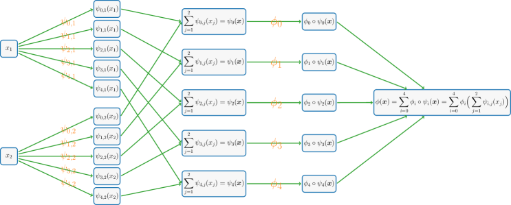
Figure 10: An illustration of the target network realizing $\phi$ for any ${\bm{x}}\in[a,b]^{d}$ in the case of $d=2$. This network contains $(2d+1)d+(2d+1)=(d+1)(2d+1)$ sub-networks that realize $\psi_{i,j}$ and $\phi_{i}$ for $i=0,1,{\cdots},2d$ and $j=1,2,{\cdots},d$.

Fix ${\bm{x}}\in[a,b]^{d}$ and $i\in\{0,1,{\cdots},2d\}$. Recall that $h_{i}({\bm{x}})\in[\tfrac{1}{4},\tfrac{3}{4}]$ and

$$|h_{i}({\bm{x}})-\psi_{i}({\bm{x}})|<\delta\leq\tfrac{1}{4},$$

implying $\psi_{i}({\bm{x}})\in[0,1]$. Then, by Equation (12) (set $z_{1}=h_{i}({\bm{x}})$ and $z_{2}=\psi_{i}({\bm{x}})$ therein), we have

$$\Big{|}g_{i}\circ h_{i}({\bm{x}})-g_{i}\circ\psi_{i}({\bm{x}})\Big{|}=\Big{|}g_{i}\big{(}h_{i}({\bm{x}})\big{)}-g_{i}\big{(}\psi_{i}({\bm{x}})\big{)}\Big{|}<\varepsilon/(4d+2).$$

By Equation (13) (set $z=\psi_{i}({\bm{x}})\in[0,1]$ therein), we have

$$\Big{|}g_{i}\circ\psi_{i}({\bm{x}})-\phi_{i}\circ\psi_{i}({\bm{x}})\Big{|}=\Big{|}g_{i}\big{(}\psi_{i}({\bm{x}})\big{)}-\phi_{i}\big{(}\psi_{i}({\bm{x}})\big{)}\Big{|}<\varepsilon/(4d+2).$$

Therefore, for any ${\bm{x}}\in[a,b]^{d}$, we have

$$\begin{split}\big{|}f({\bm{x}})-\phi({\bm{x}})\big{|}&=\Big{|}\sum_{i=0}^{2d}g_{i}\circ h_{i}({\bm{x}})-\sum_{i=0}^{2d}\phi_{i}\circ\psi_{i}({\bm{x}})\Big{|}=\sum_{i=0}^{2d}\Big{|}g_{i}\circ h_{i}({\bm{x}})-\phi_{i}\circ\psi_{i}({\bm{x}})\Big{|}\\ &\leq\sum_{i=0}^{2d}\bigg{(}\Big{|}g_{i}\circ h_{i}({\bm{x}})-g_{i}\circ\psi_{i}({\bm{x}})\Big{|}+\Big{|}g_{i}\circ\psi_{i}({\bm{x}})-\phi_{i}\circ\psi_{i}({\bm{x}})\Big{|}\bigg{)}\\ &<\sum_{i=0}^{2d}\Big{(}\varepsilon/(4d+2)+\varepsilon/(4d+2)\Big{)}=\varepsilon.\end{split}$$

It remains to show $\phi$ can be generated by an EUAF network with the desired size. Recall that, for each $i\in\{0,1,{\cdots},2d\}$ and each $j\in\{1,2,{\cdots},d\}$, $\psi_{i,j}$ can be generated by an EUAF network with width $36$, depth $5$, and therefore at most

$$(1\times 36+36)\ +\ (36\times 36+36)\times 4\ +\ (36\times 1+1)=5437$$

nonzero parameters. Hence, for each $i\in\{0,1,{\cdots},2d\}$, $\psi_{i}$, given by $\psi_{i}({\bm{x}})=\sum_{j=1}^{d}\psi_{i,j}(x_{j})$, can be generated by an EUAF network with width $36d$, depth $5$, and at most $5437d$ nonzero parameters.

Since $\psi_{i}({\bm{x}})\in[0,1]$ for any ${\bm{x}}\in[a,b]^{d}$ and $i=0,1,{\cdots},2d$, we have $\sigma\big{(}\psi_{i}({\bm{x}})\big{)}=\psi_{i}({\bm{x}})$ for any ${\bm{x}}\in[a,b]^{d}$. Hence, $\phi_{i}\circ\psi_{i}$ can be generated by an EUAF network as visualized in Figure 11.

Figure 11: An illustration of the target EUAF network generating $\phi_{i}\circ\psi_{i}({\bm{x}})$ for any ${\bm{x}}\in[a,b]^{d}$ and $i=0,1,{\cdots},2d$.

Recall that $\phi_{i}$ can be generated by an EUAF network with width $36$ and depth $5$. Hence, the network generating $\phi_{i}$ has at most $5437$ nonzero parameters. As we can see from Figure 11, $\phi_{i}\circ\psi_{i}$ can be generated by an EUAF network with width $\max\{36d,36\}=36d$, depth $5+1+5=11$, and at most $5437d+5437=5437(d+1)$ nonzero parameters. This means $\phi=\sum_{i=0}^{2d}\phi_{i}\circ\psi_{i}$ can be generated by an EUAF network with width $36d(2d+1)$, depth $11$, and therefore at most $5437(d+1)(2d+1)$ nonzero parameters as desired. So we finish the proof.

5.2 Proof of Theorem 4

The proof of Theorem 4 relies on a basic result of real analysis given in the following lemma.

Lemma 13.

Suppose $A,B\subseteq\mathbb{R}^{d}$ are two disjoint bounded closed sets. Then, there exists a continuous function $f\in C(\mathbb{R}^{d})$ such that $f({\bm{x}})=1$ for any ${\bm{x}}\in A$ and $f({\bm{y}})=0$ for any ${\bm{y}}\in B$.

Proof.

Define $\textnormal{dist}({\bm{x}},A)=\inf\{\|{\bm{x}}-{\bm{y}}\|_{2}:{\bm{y}}\in A\}$ and $\textnormal{dist}({\bm{x}},B)=\inf\{\|{\bm{x}}-{\bm{y}}\|_{2}:{\bm{y}}\in B\}$ for any ${\bm{x}}\in\mathbb{R}^{d}$. It is easy to verify that $\textnormal{dist}({\bm{x}},A)$ and $\textnormal{dist}({\bm{x}},B)$ are continuous in ${\bm{x}}\in\mathbb{R}^{d}$. Since $A,B\in\mathbb{R}^{d}$ are two disjoint bounded closed subsets, we have $\textnormal{dist}({\bm{x}},A)+\textnormal{dist}({\bm{x}},B)>0$ for any ${\bm{x}}\in\mathbb{R}^{d}$. Finally, define

$$f({\bm{x}})\coloneqq\frac{\textnormal{dist}({\bm{x}},B)}{\textnormal{dist}({\bm{x}},A)+\textnormal{dist}({\bm{x}},B)}\quad\textnormal{for any ${\bm{x}}\in\mathbb{R}^{d}$.}$$

Then $f$ meets the requirements. So we finish the proof. ∎

With Lemma 13, we can prove Theorem 4.

Proof of Theorem 4.

For any $f=\sum_{j=1}^{J}r_{j}\cdot{\mathds{1}}_{E_{j}}\in{\mathscr{C}}_{d}(E_{1},E_{2},{\cdots},E_{J})$, our goal is to construct a function $\phi$ generated by a $\sigma$-activated network such that $\phi({\bm{x}})=f({\bm{x}})$ for any ${\bm{x}}\in\bigcup_{j=1}^{J}E_{j}$, where $E_{1},E_{2},{\cdots},E_{J}$ are pairwise disjoint bounded closed subsets of $\mathbb{R}^{d}$. Define $E\coloneqq\bigcup_{j=1}^{J}E_{j}$ and choose $a,b\in\mathbb{R}$ properly such that $E\subseteq[a,b]^{d}$.

For each $j\in\{1,2,{\cdots},J\}$, $E_{j}$ and ${\widetilde{E}}_{j}\coloneqq E\big{\backslash}E_{j}$ are two disjoint bounded closed subsets. Then, for each $j$, by Lemma 13, there exists $g_{j}\in C(\mathbb{R}^{d})$ such that $g_{j}({\bm{x}})=1$ for any ${\bm{x}}\in E_{j}$ and $g_{j}({\bm{y}})=0$ for any ${\bm{y}}\in{\widetilde{E}}_{j}=E\backslash E_{j}$. By defining $g\coloneqq\sum_{j=1}^{J}r_{j}\cdot g_{j}\in C(\mathbb{R}^{d})$, we have $g({\bm{x}})=\sum_{j=1}^{J}r_{j}\cdot{\mathds{1}}_{E_{j}}({\bm{x}})=f({\bm{x}})$ for any ${\bm{x}}\in E=\bigcup_{j=1}^{J}E_{j}$.

Since $r_{1},r_{2},{\cdots},r_{J}$ are rational numbers and $g:[a,b]^{d}\to\mathbb{R}$ is continuous, there exist $n_{1},n_{2}\in\mathbb{Z}\backslash\{0\}$ such that

• $n_{1}\cdot r_{j}+n_{2}\in\mathbb{N}^{+}$ for $j=1,2,{\cdots},J$;

• $n_{1}\cdot g({\bm{x}})+n_{2}\geq 0$ for any ${\bm{x}}\in[a,b]^{d}$.

By applying Theorem 1 to $2(n_{1}\cdot g+n_{2})+1\in C([a,b]^{d})$, there exists a function $\phi_{1}$ generated by an EUAF network with width $36d(2d+1)$, depth $11$, and at most $5437(d+1)(2d+1)$ nonzero parameters such that

$$\Big{|}2\big{(}n_{1}\cdot g({\bm{x}})+n_{2}\big{)}+1-\phi_{1}({\bm{x}})\Big{|}\leq 1/2\quad\textnormal{for any ${\bm{x}}\in[a,b]^{d}$.}$$ (14)

It follows that

$$\Big{|}2\big{(}n_{1}\cdot\sum_{j=1}^{J}r_{j}\cdot{\mathds{1}}_{E_{j}}({\bm{x}})+n_{2}\big{)}+1-\phi_{1}({\bm{x}})\Big{|}\leq 1/2\quad\textnormal{for any ${\bm{x}}\in E=\bigcup_{j=1}^{J}E_{j}$.}$$

Since $E_{1},E_{2},{\cdots},E_{J}$ are pairwise disjoint, we have

$$\Big{|}2(n_{1}\cdot r_{j}+n_{2})+1-\phi_{1}({\bm{x}})\Big{|}\leq 1/2\quad\textnormal{for any ${\bm{x}}\in E_{j}$ and each $j\in\{1,2,{\cdots},J\}$.}$$ (15)

Define $\phi_{2}(x)=x+1/2-\sigma(x+3/2)$ for any $x\in\mathbb{R}$. See Figure 12 for an illustration.

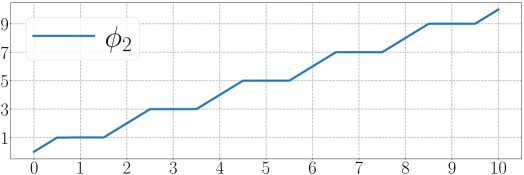
Figure 12: An illustration of $\phi_{2}$ on $[0,10]$.

It is easy to verify that

$$\phi_{2}(y)=2k+1\quad\textnormal{ for any $y$ and $k\in\mathbb{N}^{+}$ with $|2k+1-y|\leq 1/2$.}$$ (16)

Then, by Equations (15) and $\eqref{eq:phi2:2k+1}$ (set $y=\phi_{1}({\bm{x}})$ and $k=n_{1}\cdot r_{j}+n_{2}$ therein), we have

$$\phi_{2}\circ\phi_{1}({\bm{x}})=\phi_{2}(y)=2k+1=2(n_{1}\cdot r_{j}+n_{2})+1$$

for any ${\bm{x}}\in E_{j}$ and any $j\in\{1,2,{\cdots},J\}$, which implies

$$\frac{\phi_{2}\circ\phi_{1}({\bm{x}})-2n_{2}-1}{2n_{1}}=r_{j}\quad\textnormal{for any ${\bm{x}}\in E_{j}$ and any $j\in\{1,2,{\cdots},J\}$}.$$

Define

$$\phi({\bm{x}})\coloneqq\frac{\phi_{2}\circ\phi_{1}({\bm{x}})-2n_{2}-1}{2n_{1}}\quad\textnormal{ for any ${\bm{x}}\in[a,b]^{d}$. }$$

Clearly, we have $\phi({\bm{x}})=r_{j}$ for any ${\bm{x}}\in E_{j}$ and each $j\in\{1,2,{\cdots},J\}$, which implies

$$\phi({\bm{x}})=\sum_{j=1}^{J}r_{j}\cdot{\mathds{1}}_{E_{j}}({\bm{x}})=f({\bm{x}})\quad\textnormal{ for any ${\bm{x}}\in E=\bigcup_{j=1}^{J}E_{j}$.}$$

It remains to show that $\phi$ can be generated by an EUAF network with the desired size. Set $M=2\|n_{1}g+n_{2}\|_{L^{\infty}([a,b]^{d})}+3/2>0$. By Equation (14) and the fact $n_{1}\cdot g({\bm{x}})+n_{2}\geq 0$ for any ${\bm{x}}\in[a,b]^{d}$, we have

$$\phi_{1}({\bm{x}})\in\Big{[}1/2,\ 2\|n_{1}g+n_{2}\|_{L^{\infty}([a,b]^{d})}+1+1/2\Big{]}\subseteq[0,M]\quad\textnormal{for any ${\bm{x}}\in[a,b]^{d}$.}$$

Then, for any ${\bm{x}}\in[a,b]^{d}$, we have

$$\begin{split}\phi_{2}\circ\phi_{1}({\bm{x}})&=\phi_{1}({\bm{x}})+1/2-\sigma\big{(}\phi_{1}({\bm{x}})+3/2\big{)}\\ &=M\sigma\big{(}\phi_{1}({\bm{x}})/M\big{)}+1/2-\sigma\big{(}\phi_{1}({\bm{x}})+3/2\big{)}.\end{split}$$

It follows that

$$\phi({\bm{x}})=\frac{\phi_{2}\circ\phi_{1}({\bm{x}})-2n_{2}-1}{2n_{1}}=\frac{M\sigma\big{(}\phi_{1}({\bm{x}})/M\big{)}-\sigma\big{(}\phi_{1}({\bm{x}})+3/2\big{)}-2n_{2}-1/2}{2n_{1}},$$

for any ${\bm{x}}\in[a,b]^{d}$. That means the network realizing $\phi$ has just one more hidden layer with $2$ neurons, compared to the network realizing $\phi_{1}$. Recall that $\phi_{1}$ can be generated by an EUAF network with width $36d(2d+1)$, depth $11$, and at most $5437(d+1)(2d+1)$ nonzero parameters. Therefore, $\phi$, limited on $[a,b]^{d}$, can be generated by an EUAF network with width $36d(2d+1)$, depth $12$, and at most

$$5437(d+1)(2d+1)\ +\ \underbrace{2\times 36d(2d+1)+2\ +\ 2\times 1+1}_{\textnormal{all possible new parameters}}\leq 5509(d+1)(2d+1)$$

nonzero parameters. So we finish the proof. ∎

6 Proof of Theorem 6

To prove Theorem 6, we need to introduce two auxiliary theorems, Theorems 14 and 15, which serve as two important intermediate steps.

Theorem 14.

Let $f\in C([0,1])$ be a continuous function. Given any $\varepsilon>0$, if $K$ is a positive integer satisfying

$$|f(x_{1})-f(x_{2})|<\varepsilon/2\quad\textnormal{for any $x_{1},x_{2}\in[0,1]$ with $|x_{1}-x_{2}|<1/K$,}$$ (17)

then there exists a function $\phi$ generated by an EUAF network with width $2$ and depth $3$ such that $\|\phi\|_{L^{\infty}([0,1])}\leq\|f\|_{L^{\infty}([0,1])}+1$ and

$$|\phi(x)-f(x)|<\varepsilon\quad\textnormal{for any}\ x\in\bigcup_{k=0}^{K-1}\big{[}\tfrac{2k}{2K},\tfrac{2k+1}{2K}\big{]}.$$

Theorem 15.

Let $f\in C([0,1])$ be a continuous function. Then, for any $\varepsilon>0$, there exists a function $\phi$ generated by an EUAF network with width $36$ and depth $5$ such that

$$|\phi(x)-f(x)|<\varepsilon\quad\textnormal{for any $x\in[0,\tfrac{9}{10}]$. }$$

To prove Theorem 14, we only need to care about the approximation on one “half” of $[0,1]$. It is not necessary to care about the approximation on the other “half” of $[0,1]$. Such an idea is similar to the “trifling region” in (Lu et al., 2021; Zhang, 2020). As we shall see later, the proof of Theorem 14 can eventually be converted to a point-fitting problem, which can be solved by applying Proposition 7.

The key idea to prove Theorem 15 is to apply Theorem 14 to several horizontally shifted variants of the target function. Then a good approximation can be constructed via the combinations and multiplications of these variants, similar to the idea of (Lu et al., 2021; Zhang, 2020) to obtain an error estimation with the $L^{\infty}$-norm from a result with the $L^{p}$-norm for $p\in[1,\infty)$.

The proofs of Theorems 14 and 15 will be presented in Sections 6.1 and 6.2, respectively. Let us first prove Theorem 6 by assuming Theorem 15 is true.

Proof of Theorem 6.

Define a linear function ${\mathcal{L}}$ by ${\mathcal{L}}(x)=a+\tfrac{10(b-a)}{9}x$ for any $x\in[0,\tfrac{9}{10}]$. Then ${\mathcal{L}}$ is a bijection from $[0,\tfrac{9}{10}]$ to $[a,b]$. It follows that $f\circ{\mathcal{L}}$ is a continuous function on $[0,\tfrac{9}{10}]$. By Theorem 15, there exists a function ${\widetilde{\phi}}$ generated by an EUAF network with width $36$ and depth $5$ such that

$$|f\circ{\mathcal{L}}(x)-{\widetilde{\phi}}(x)|<\varepsilon\quad\textnormal{for any $x\in[0,\tfrac{9}{10}]$.}$$

Define $\widetilde{{\mathcal{L}}}(y)=\tfrac{9(y-a)}{10(b-a)}$ for any $y\in[a,b]$. Clearly, it is the inverse of ${\mathcal{L}}$, i.e., ${\mathcal{L}}\circ\widetilde{{\mathcal{L}}}(y)=y$ for any $y\in[a,b]$. Therefore, for any $y\in[a,b]$, we have $x=\widetilde{{\mathcal{L}}}(y)\in[0,\tfrac{9}{10}]$, which implies

$$\begin{split}|f(y)-{\widetilde{\phi}}\circ\widetilde{{\mathcal{L}}}(y)|&=\big{|}f\circ{\mathcal{L}}\circ\widetilde{{\mathcal{L}}}(y)-{\widetilde{\phi}}\circ\widetilde{{\mathcal{L}}}(y)\big{|}\\ &=\Big{|}f\circ{\mathcal{L}}\big{(}\widetilde{{\mathcal{L}}}(y)\big{)}-{\widetilde{\phi}}\big{(}\widetilde{{\mathcal{L}}}(y)\big{)}\Big{|}=|f\circ{\mathcal{L}}(x)-{\widetilde{\phi}}(x)|<\varepsilon.\end{split}$$

By defining $\phi\coloneqq{\widetilde{\phi}}\circ\widetilde{{\mathcal{L}}}$, we have $|f(y)-\phi(y)|<\varepsilon$ for any $y\in[a,b]$ as desired.

Note that ${\widetilde{\phi}}$ can be realized by an EUAF network with width $36$ and depth $5$. We can compose $\widetilde{{\mathcal{L}}}$ and the affine linear map of the network ${\widetilde{\phi}}$ that connects the input layer and the first hidden layer. Therefore, $\phi={\widetilde{\phi}}\circ\widetilde{{\mathcal{L}}}$ can also be realized by an EUAF network with width $36$ and depth $5$. So we finish the proof. ∎

6.1 Proof of Theorem 14

Partition $[0,1]$ into $2K$ small intervals ${\mathcal{I}}_{k}$ and ${\mathcal{\widetilde{I}}}_{k}$ for $k=1,2,{\cdots},K$, i.e.,

$${\mathcal{I}}_{k}=\big{[}\tfrac{2k-2}{2K},\tfrac{2k-1}{2K}\big{]}\quad\textnormal{and}\quad{\mathcal{\widetilde{I}}}_{k}=\big{[}\tfrac{2k-1}{2K},\tfrac{2k}{2K}\big{]}.$$

Clearly, $[0,1]=\bigcup_{k=1}^{K}({\mathcal{I}}_{k}\cup{\mathcal{\widetilde{I}}}_{k})$. Let $x_{k}$ be the right endpoint of ${\mathcal{I}}_{k}$, i.e., $x_{k}=\tfrac{2k-1}{2K}$ for $k=1,2,{\cdots},K$. See an illustration of ${\mathcal{I}}_{k}$, ${\mathcal{\widetilde{I}}}_{k}$, and $x_{k}$ in Figure 13 for the case $K=5$.

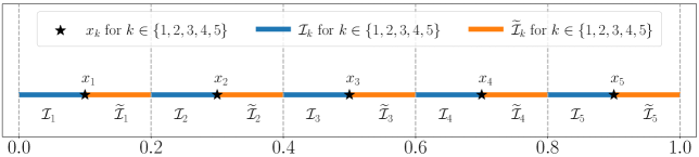
Figure 13: An illustration of ${\mathcal{I}}_{k}$ and ${\mathcal{\widetilde{I}}}_{k}$ for $k\in\{1,2,{\cdots},K\}$ with $K=5$.

Our goal is to construct a function $\phi$ generated by an EUAF network with the desired size to approximate $f$ well on ${\mathcal{I}}_{k}$ for $k=1,2,{\cdots},K$. It is not necessary to care about the values of $\phi$ on ${\mathcal{\widetilde{I}}}_{k}$ for all $k$. In other words, we only need to care about the approximation on one “half” of $[0,1]$, which is the key for our proof.

Define $\psi(x)\coloneqq x-\sigma(x)$ for any $x\in\mathbb{R}$, where $\sigma$ is defined in Equation (1). See Figure 14 for an illustration of $\psi$.

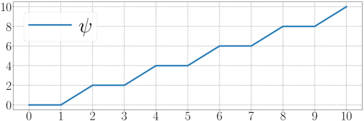
Figure 14: An illustration of $\psi$ on $[0,10]$.

It is easy to verify that

$$\psi(y)=2k-2\quad\textnormal{ for any $y\in[2k-2,2k-1]$ and each $k\in\{1,2,{\cdots},K\}$.}$$

It follows that

$$\psi(2Kx)/2+1=k\quad\textnormal{for any $x\in[\tfrac{2k-2}{2K},\tfrac{2k-1}{2K}]={\mathcal{I}}_{k}$ and each $k\in\{1,2,{\cdots},K\}$.}$$ (18)

Recall that $x_{k}$ is the right endpoint of ${\mathcal{I}}_{k}$ for $k=1,2,{\cdots},K$. Set $M=\|f\|_{L^{\infty}([0,1])}+1$ and define

$$\xi_{k}\coloneqq\tfrac{f(x_{k})+M}{2M}\in[0,1]\quad\textnormal{ for $k=1,2,{\cdots},K.$}$$

Then $[\xi_{1},\xi_{2},{\cdots},\xi_{K}]^{T}$ is in $[0,1]^{K}$. By Proposition 7, there exists $w_{0}\in\mathbb{R}$ such that

$$\big{|}\sigma_{1}(\tfrac{w_{0}}{\pi+k})-\xi_{k}\big{|}<\varepsilon/(4M)\quad\textnormal{for $k=1,2,{\cdots},K$.}$$

Let $m_{0}$ be an integer larger than $|w_{0}|$, e.g., set $m_{0}=\lfloor|w_{0}|\rfloor+1$. It is easy to verify that

$$\tfrac{w_{0}}{\pi+k}+2m_{0}\geq 0\quad\textnormal{ for any $x\in[0,1]$.}$$

Since $\sigma(x)=\sigma_{1}(x)$ for any $x\geq 0$ and $\sigma_{1}$ is periodic with period $2$, we have

$$\big{|}\sigma(\tfrac{w_{0}}{\pi+k}+2m_{0})-\xi_{k}\big{|}=\big{|}\sigma_{1}(\tfrac{w_{0}}{\pi+k}+2m_{0})-\xi_{k}\big{|}=\big{|}\sigma_{1}(\tfrac{w_{0}}{\pi+k})-\xi_{k}\big{|}<\varepsilon/(4M),$$

for $k=1,2,{\cdots},K$. It follows that

$$\begin{split}\Big{|}2M\sigma(\tfrac{w_{0}}{\pi+k}+2m_{0})-M-f(x_{k})\Big{|}&=\Big{|}2M\sigma(\tfrac{w_{0}}{\pi+k}+2m_{0})-M-(2M\xi_{k}-M)\Big{|}\\ &=2M\big{|}\sigma(\tfrac{w_{0}}{\pi+k}+2m_{0})-\xi_{k}\big{|}<2M\cdot\tfrac{\varepsilon}{4M}=\varepsilon/2,\end{split}$$ (19)

for $k=1,2,{\cdots},K$.

The desired $\phi$ is defined as

$$\phi(x)\coloneqq 2M\sigma\big{(}\tfrac{w_{0}}{\pi+\psi(2Kx)/2+1}+2m_{0}\big{)}-M\quad\textnormal{for any $x\in[0,1]$}.$$

Recall that $m_{0}\geq|w_{0}|$ and $\psi(x)\geq 0$ for any $x\geq 0$, which implies

$$\tfrac{w_{0}}{\pi+\psi(2Kx)/2+1}+2m_{0}\geq 0\quad\textnormal{ for any $x\in[0,1]$.}$$

It follows that $\|\phi\|_{L^{\infty}([0,1])}\leq M=\|f\|_{L^{\infty}([0,1])}+1$ since $0\leq\sigma(y)\leq 1$ for any $y\geq 0$.

For any $x\in{\mathcal{I}}_{k}$ and each $k\in\{1,2,{\cdots},K\}$, by Equation (18), we have $\psi(2Kx)/2+1=k$, which implies

$$\phi(x)=2M\sigma\big{(}\tfrac{w_{0}}{\pi+\psi(2Kx)/2+1}+2m_{0}\big{)}-M=2M\sigma\big{(}\tfrac{w_{0}}{\pi+k}+2m_{0}\big{)}-M.$$

Clearly, for any $x\in{\mathcal{I}}_{k}$ and each $k\in\{1,2,{\cdots},K\}$, we have $|x_{k}-x|<1/K$. Then, by Equation (17), we get

$$|f(x_{k})-f(x)|<\varepsilon/2\quad\textnormal{for any $x\in{\mathcal{I}}_{k}$ and each $k\in\{1,2,{\cdots},K\}$.}$$

Therefore, by Equation (19), we have

$$\begin{split}|\phi(x)-f(x)|&=\Big{|}2M\sigma\big{(}\tfrac{w_{0}}{\pi+k}+2m_{0}\big{)}-M-f(x)\Big{|}\\ &\leq\Big{|}2M\sigma\big{(}\tfrac{w_{0}}{\pi+k}+2m_{0}\big{)}-M-f(x_{k})\Big{|}+\big{|}f(x_{k})-f(x)\big{|}<\varepsilon/2+\varepsilon/2=\varepsilon\end{split}$$

for any $x\in{\mathcal{I}}_{k}$ and each $k\in\{1,2,{\cdots},K\}$. It follows that

$$\begin{split}|\phi(x)-f(x)|<\varepsilon\quad\textnormal{for any $x\in\bigcup_{j=1}^{K}{\mathcal{I}}_{j}=\bigcup_{j=1}^{K}\big{[}\tfrac{2j-2}{2K},\tfrac{2j-1}{2K}\big{]}=\bigcup_{k=0}^{K-1}\big{[}\tfrac{2k}{2K},\tfrac{2k+1}{2K}\big{]}$}.\end{split}$$

It remains to show that $\phi$ can be generated by an EUAF network with the desired size. Observe that

$$\sigma(y)+1=\frac{y}{|y|+1}+1=\frac{y}{-y+1}+1=\frac{1}{-y+1}\quad\textnormal{for any $y\leq 0$.}$$

By setting $y=-\pi-\psi(2Kx)/2\leq 0$ for any $x\in[0,1]$, we have

$$\begin{split}\frac{1}{\pi+\psi(2Kx)/2+1}=\frac{1}{-y+1}=\sigma(y)+1&=\sigma\big{(}-\pi-\psi(2Kx)/2\big{)}+1\\ &=\sigma\Big{(}-\pi-\big{(}2Kx-\sigma(2Kx)\big{)}/2\Big{)}+1\\ &=\sigma\big{(}-\pi-Kx+\sigma(2Kx)/2\big{)}+1,\end{split}$$

where the second-to-last equality comes from $\psi(z)=z-\sigma(z)$ for any $z\in\mathbb{R}$. Therefore, we get

$$\begin{split}\phi(x)&=2M\sigma\big{(}\tfrac{w_{0}}{\pi+\psi(2Kx)/2+1}+2m_{0}\big{)}-M\\ &=2M\sigma\Big{(}w_{0}\sigma\big{(}-\pi-Kx+\sigma(2Kx)/2\big{)}+w_{0}+2m_{0}\Big{)}-M.\end{split}$$ (20)

Figure 15: An illustration of the target EUAF network realizing $\phi(x)$ for $x\in[0,1]$ based on Equation (20).

Thus, the desired EUAF network realizing $\phi$ is shown in Figure 15. Clearly, the network in Figure 15 has width $2$ and depth $3$ as desired. It is easy to verify that the network architecture corresponding $\phi$ is independent of the target function $f$ and the desired error $\varepsilon$. That is, we can fix the architecture and only adjust parameters to achieve the desired approximation error. So we finish the proof.

6.2 Proof of Theorem 15

The key idea of proving Theorem 15 is to apply Theorem 14 to several horizontally shifted variants of the target function. Then a good approximation can be expected via combinations and multiplications of these variants. Thus, we need to reproduce $f(x,y)=xy$ locally via an EUAF network as shown in the following lemma.

Lemma 16.

For any $M>0$, there exists a function $\phi$ generated by an EUAF network with width $9$ and depth $2$ such that

$$\phi(x,y)=xy\quad\textnormal{for any $x,y\in[-M,M]$.}$$

The proof of this lemma is given in Section 6.3. Now let us first prove Theorem 15 by assuming this lemma is true.

Proof of Theorem 15.

Set $\widetilde{\varepsilon}=\varepsilon/4$ and extend $f$ from $[0,1]$ to $[-1,1]$ by defining $f(x)=f(0)$ for any $x\in[-1,0)$. Then $f$ is continuous on $[-1,1]$ and therefore uniformly continuous. Thus, there exists $K=K(f,\varepsilon)\in\mathbb{N}^{+}$ with $K\geq 10$ such that

$$|f(x_{1})-f(x_{2})|<\widetilde{\varepsilon}/2\quad\textnormal{for any $x_{1},x_{2}\in[-1,1]$ with $|x_{1}-x_{2}|<1/K$.}$$

For $i=1,2,3,4$, define

$$f_{i}(x)\coloneqq f\big{(}x-\tfrac{i}{4K}\big{)}\quad\textnormal{for any $x\in[0,1]$.}$$

For each $i\in\{1,2,3,4\}$ and any $x_{1},x_{2}\in[0,1]$ with $|x_{1}-x_{2}|<1/K$, we have $x_{1}-\tfrac{i}{4K},x_{2}-\tfrac{i}{4K}\in[-1,1]$ and $\big{|}(x_{1}-\tfrac{i}{4K})-(x_{2}-\tfrac{i}{4K})\big{|}=|x_{1}-x_{2}|<1/K$, which implies

$$|f_{i}(x_{1})-f_{i}(x_{2})|=\big{|}f(x_{1}-\tfrac{i}{4K})-f(x_{2}-\tfrac{i}{4K})\big{|}<\widetilde{\varepsilon}/2.$$

That is, for $i=1,2,3,4$, we have

$$|f_{i}(x_{1})-f_{i}(x_{2})|<\widetilde{\varepsilon}/2\quad\textnormal{for any $x_{1},x_{2}\in[0,1]$ with $|x_{1}-x_{2}|<1/K$,}$$

which means we can apply Theorem 14 to $f_{i}\in C([0,1])$. For each $i\in\{1,2,3,4\}$, by Theorem 14, there exists a function $\phi_{i}$ generated by an EUAF network with width $2$ and depth $3$ such that

$$\|\phi_{i}\|_{L^{\infty}([0,1])}\leq\|f_{i}\|_{L^{\infty}([0,1])}+1\leq\|f\|_{L^{\infty}([-1,1])}+1$$

and

$$\big{|}\phi_{i}(x)-f_{i}(x)\big{|}<\widetilde{\varepsilon}=\varepsilon/4\quad\textnormal{for any}\ x\in\bigcup_{k=0}^{K-1}\big{[}\tfrac{2k}{2K},\tfrac{2k+1}{2K}\big{]}.$$

Define

$$\psi(x)=\sigma\big{(}x+1-\sigma(x+1)\big{)}\quad\textnormal{for any $x\in\mathbb{R}$.}$$

See an illustration of $\psi$ on $[0,2K]$ for $K=5$ in Figure 16.

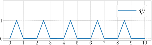
Figure 16: An illustration of $\psi$ on $[0,2K]$ for $K=5$.

Clearly, $0\leq\psi(2Kx)\leq 1$ for any $x\in[0,1]$, from which we deduce

$$\Big{|}\big{(}\phi_{i}(x)-f_{i}(x)\big{)}\psi(2Kx)\Big{|}\leq\big{|}\phi_{i}(x)-f_{i}(x)\big{|}<\varepsilon/4\quad\textnormal{for any}\ x\in\bigcup_{k=0}^{K-1}\big{[}\tfrac{2k}{2K},\tfrac{2k+1}{2K}\big{]}.$$

Observe that $\psi(y)=0$ for $y\in\bigcup_{k=0}^{K-1}[{2k+1},{2k+2}]$, which implies

$$\psi(2Kx)=0\quad\textnormal{for any $x\in\bigcup_{k=0}^{K-1}[\tfrac{2k+1}{2K},\tfrac{2k+2}{2K}]\supseteq[0,1]\Big{\backslash}\bigcup_{k=0}^{K-1}\big{[}\tfrac{2k}{2K},\tfrac{2k+1}{2K}\big{]}$}.$$

It follows that

$$\Big{|}\big{(}\phi_{i}(x)-f_{i}(x)\big{)}\psi(2Kx)\Big{|}<\varepsilon/4\quad\textnormal{for any $x\in[0,1]$ and $i=1,2,3,4$}.$$ (21)

For each $i\in\{1,2,3,4\}$ and any $z\in[0,\tfrac{9}{10}]\subseteq[0,1-\tfrac{1}{K}]\subseteq[0,1-\tfrac{i}{4K}]$, we have

$$y_{i}=z+\tfrac{i}{4K}\in[\tfrac{i}{4K},1]\subseteq[0,1].$$

Therefore, by bringing $x=y_{i}\in[0,1]$ into Equation (21), we have

$$\begin{split}\varepsilon/4&>\Big{|}\big{(}\phi_{i}(y_{i})-f_{i}(y_{i})\big{)}\psi(2Ky_{i})\Big{|}=\Big{|}\phi_{i}(y_{i})\psi(2Ky_{i})-f_{i}(y_{i})\psi(2Ky_{i})\Big{|}\\ &=\Big{|}\phi_{i}(z+\tfrac{i}{4K})\psi\big{(}2K(z+\tfrac{i}{4K})\big{)}-f_{i}(z+\tfrac{i}{4K})\psi\big{(}2K(z+\tfrac{i}{4K})\big{)}\Big{|}\\ &=\Big{|}\phi_{i}(z+\tfrac{i}{4K})\psi\big{(}2Kz+\tfrac{i}{2}\big{)}-f(z)\psi\big{(}2Kz+\tfrac{i}{2}\big{)}\Big{|}\end{split}$$ (22)

for any $z\in[0,\tfrac{9}{10}]$, where the last equality comes from the fact that $f_{i}(x)=f(x-\tfrac{i}{4K})$ for any $x\in[0,1]\supseteq[\tfrac{i}{4K},1]$. The desired $\phi$ is defined as

$$\phi(x)\coloneqq\sum_{i=1}^{4}\phi_{i}(x+\tfrac{i}{4K})\psi\big{(}2Kx+\tfrac{i}{2}\big{)}\quad\textnormal{for any $x\in[0,\tfrac{9}{10}]$.}$$

It is easy to verify that $\sum_{i=1}^{4}\psi\big{(}x+\tfrac{i}{2}\big{)}=1$ for any $x\geq 0$ based on the definition of $\psi$. See Figure 17 for illustrations. It follows that $\sum_{i=1}^{4}\psi\big{(}2Kz+\tfrac{i}{2}\big{)}=1$ for any $z\in[0,\tfrac{9}{10}]$.

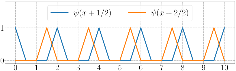
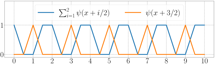
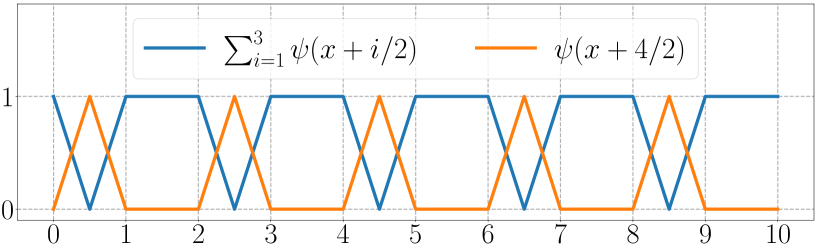
Figure 17: Illustrations of $\sum_{i=1}^{4}\psi(x+i/2)=1$ for any $x\in[0,10]$.

Hence, for any $z\in[0,\tfrac{9}{10}]$, by Equation (22), we have

$$\begin{split}\big{|}\phi(z)-f(z)\big{|}&=\Big{|}\sum_{i=1}^{4}\phi_{i}(z+\tfrac{i}{4K})\psi\big{(}2Kz+\tfrac{i}{2}\big{)}-f(z)\sum_{i=1}^{4}\psi\big{(}2Kz+\tfrac{i}{2}\big{)}\Big{|}\\ &\leq\sum_{i=1}^{4}\Big{|}\phi_{i}(z+\tfrac{i}{4K})\psi\big{(}2Kz+\tfrac{i}{2}\big{)}-f(z)\psi\big{(}2Kz+\tfrac{i}{2}\big{)}\Big{|}<4\cdot\frac{\varepsilon}{4}=\varepsilon.\end{split}$$

That is, $|\phi(x)-f(x)|<\varepsilon$ for any $x\in[0,\tfrac{9}{10}]$ as desired. It remains to show that $\phi$, limited on $[0,\tfrac{9}{10}]$, can be generated by an EUAF network with the desired size.

Note that $x+1=(2K+1)\sigma(\tfrac{x+1}{2K+1})$ for any $x\in[0,2K]$, which implies

$$\psi(x)=\sigma\big{(}x+1-\sigma(x+1)\big{)}=\sigma\Big{(}(2K+1)\sigma(\tfrac{x+1}{2K+1})-\sigma(x+1)\Big{)}.$$

This means $\psi$, limited on $[0,2K]$, can be generated by an EUAF network with width $2$ and depth $2$. Since $0\leq 2Kx+\tfrac{i}{2}\leq 2K\tfrac{9}{10}+2=2K(\tfrac{9}{10}+\tfrac{1}{K})\leq 2K$ for any $x\in[0,\tfrac{9}{10}]$, $\psi(2K\cdot+\tfrac{i}{2})$, limited on $[0,\tfrac{9}{10}]$, can also be generated by an EUAF network with width $2$ and depth $2$.

Note that $\phi_{i}$, limited on $[0,1]$, can also be generated by an EUAF network with width $2$ and depth $3$. Clearly, $x+\tfrac{i}{4K}\in[0,1]$ for any $x\in[0,\tfrac{9}{10}]$, and, therefore, $\phi_{i}(\cdot+\tfrac{i}{4K})$, limited on $[0,\tfrac{9}{10}]$, can also be generated by an EUAF network with width $2$ and depth $3$.

Recall that $\|\phi_{i}\|_{L^{\infty}([0,1])}\leq\|f\|_{L^{\infty}([-1,1])}+1\eqqcolon M$. Thus, $|\phi_{i}(x+\tfrac{i}{4K})|\leq M$ and $|\psi(2Kx+\tfrac{i}{2})|\leq 1\leq M$ for any $x\in[0,\tfrac{9}{10}]$ and $i=1,2,3,4$. By Lemma 16, there exists a function $\Gamma$ generated by an EUAF network with width $9$ and depth $2$ such that

$$\Gamma(x,y)=xy\quad\textnormal{for any $x,y\in[-M,M]$.}$$

It follows that

$$\Gamma\Big{(}\phi_{i}(x+\tfrac{i}{4K}),\psi\big{(}2Kx+\tfrac{i}{2}\big{)}\Big{)}=\phi_{i}(x+\tfrac{i}{4K})\psi\big{(}2Kx+\tfrac{i}{2}\big{)}\quad\textnormal{for $i=1,2,3,4$.}$$

Figure 18: An illustration of the target EUAF network realizing each component of $\phi(x)$, $\phi_{i}(x+\tfrac{i}{4K})\psi\big{(}2Kx+\tfrac{i}{2}\big{)}$, for any $x\in[0,\tfrac{9}{10}]$ and each $i\in\{1,2,3,4\}$. The networks realizing $\phi_{i}(\cdot+\tfrac{i}{4K})$ and $\psi\big{(}2K\cdot+\tfrac{i}{2}\big{)}$ can be placed in parallel since we can manually add a hidden layers to $\psi$ since $\sigma\circ\psi\big{(}2Kx+\tfrac{i}{2}\big{)}=\psi\big{(}2Kx+\tfrac{i}{2}\big{)}$ for any $x\in[0,\tfrac{9}{10}]$.

Therefore, each component of $\phi(x)$, $\phi_{i}(x+\tfrac{i}{4K})\psi\big{(}2Kx+\tfrac{i}{2}\big{)}$ for each $i\in\{1,2,3,4\}$, can be generated by the network in Figure 18 for any $x\in[0,\tfrac{9}{10}]$. Clearly, such a network has width $9$ and depth $6$. Since the $4$-th hidden layer of the network in Figure 18 uses the identity map as an activation function for each neuron in this hidden layer, we can reduce the depth by $1$ via composing two adjacent affine linear maps to generate a new one. Thus, the network in Figure 18 can be interpreted as an EUAF network with width $9$ and depth $5$.

Note that $\phi$ is the sum of its four components, namely,

$$\phi(x)=\sum_{i=1}^{4}\phi_{i}(x+\tfrac{i}{4K})\psi\big{(}2Kx+\tfrac{i}{2}\big{)}\quad\textnormal{ for any $x\in[0,\tfrac{9}{10}]$.}$$

Therefore, $\phi$, limited on $[0,\tfrac{9}{10}]$, can be generated by an EUAF network with width $9\times 4=36$ and depth $5$ as desired. It is easy to verify that the designed network architecture is independent of the target function $f$ and the desired error $\varepsilon$. That is, we can fix the architecture and only adjust parameters to achieve an arbitrarily small approximation error. So we finish the proof. ∎

6.3 Proof of Lemma 16

The key idea of proving Lemma 16 is the polarization identity $2xy=(x+y)^{2}-x^{2}-y^{2}$. Thus, we need to reproduce $x^{2}$ locally by an EUAF network as shown in the following lemma.

Lemma 17.

There exists a function $\phi$ generated by an EUAF network with width $3$ and depth $2$ such that

$$\phi(x)=x^{2}\quad\textnormal{for any $x\in[-1,1]$.}$$

Proof.

Observe that

$$\sigma(y)+1=\frac{y}{|y|+1}+1=\frac{y}{-y+1}+1=\frac{1}{-y+1}\quad\textnormal{for any $y\leq 0$.}$$

For any $x\in[-1,1]$, we have $-x-1\leq 0$ and $-x-2\leq 0$, which implies

$$\begin{split}\sigma(-x-1)-\sigma(-x-2)&=\Big{(}\sigma(-x-1)+1\Big{)}-\Big{(}\sigma(-x-2)+1\Big{)}\\ &=\frac{1}{-(-x-1)+1}-\frac{1}{-(-x-2)+1}\\ &=\frac{1}{x+2}-\frac{1}{x+3}=\frac{1}{(x+2)(x+3)}.\end{split}$$

It follows from $1-\tfrac{12}{(x+2)(x+3)}\leq 0$ for any $x\in[-1,1]$ that

$$\begin{split}\sigma\Big{(}1-\frac{12}{(x+2)(x+3)}\Big{)}+1=\frac{1}{-\big{(}1-\tfrac{12}{(x+2)(x+3)}\big{)}+1}=\frac{x^{2}+5x+6}{12},\end{split}$$

implying

$$\begin{split}x^{2}&=12\sigma\Big{(}1-\frac{12}{(x+2)(x+3)}\Big{)}+12-(5x+6)\\ &=12\sigma\Big{(}1-12\big{(}\sigma(-x-1)-\sigma(-x-2)\big{)}\Big{)}+11\frac{6-5x}{11}\\ &=12\sigma\Big{(}1-12\sigma(-x-1)+12\sigma(-x-2)\Big{)}+11\sigma\Big{(}\frac{6-5x}{11}\Big{)}\eqqcolon\phi(x),\end{split}$$

where the equality $\tfrac{6-5x}{11}=\sigma\big{(}\tfrac{6-5x}{11}\big{)}$ comes from two facts: $\tfrac{6-5x}{11}\in[0,1]$ since $x\in[-1,1]$ and $\sigma(z)=z$ for any $z\in[0,1]$.

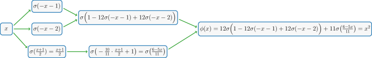
Figure 19: An illustration of the target EUAF network realizing $\phi(x)=x^{2}$ for $x\in[-1,1]$.

Then, $x^{2}$ can be generated by the network shown in Figure 19 for any $x\in[-1,1]$. The target network has width $3$ and depth $2$. So we finish the proof. ∎

With Lemma 17 at hand, we are ready to prove Lemma 16.

Proof of Lemma 16.

By Lemma 17, there exists a function ${\widetilde{\phi}}$ generated by an EUAF network such that ${\widetilde{\phi}}(t)=t^{2}$ for any $t\in[-1,1]$. Then, for any $x,y\in[-M,M]$, we have

$$\begin{split}xy&=2M^{2}\Big{(}\big{(}\tfrac{x+y}{2M}\big{)}^{2}-\big{(}\tfrac{x}{2M}\big{)}^{2}-\big{(}\tfrac{y}{2M}\big{)}^{2}\Big{)}\\ &=2M^{2}\Big{(}{\widetilde{\phi}}\big{(}\tfrac{x+y}{2M}\big{)}-{\widetilde{\phi}}\big{(}\tfrac{x}{2M}\big{)}-{\widetilde{\phi}}\big{(}\tfrac{y}{2M}\big{)}\Big{)}\eqqcolon\phi(x,y).\end{split}$$

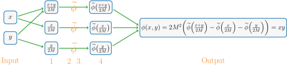
Figure 20: An illustration of the target network realizing $\phi(x)=xy$ for $x,y\in[-M,M]$.

The target network realizing $\phi$ with width $9$ and depth $4$ is shown in Figure 20. Note that we can reduce the depth by one if the activation function of each neuron in a hidden layer is the identity map. In fact, we can eliminate this hidden layer by composing two adjacent affine linear maps to generate a new one. The $1$-st and $4$-th hidden layers of the network in Figure 20 use the identity map as an activation function for each neuron. Thus, the network in Figure 20 can be interpreted as an EUAF network with width $9$ and depth $2$. So we finish the proof. ∎

7 Proof of Proposition 7

We will prove Proposition 7 in this section. The proof includes two main steps. First, we show how to simply generate a set of rationally independent numbers in Lemma 18 below. Next, we prove that the target point set via a winding of the generated rationally independent numbers is dense in a hypercube. Such a proof relies on the fact that an irrational winding on the torus is dense (e.g., see Lemma $2$ of (Yarotsky, 2021)) as shown in Lemma 19 below.

Lemma 18.

Given any $K\in\mathbb{N}^{+}$, any transcendental number $\alpha\in\mathbb{R}\backslash\mathbb{A}$, and any pairwise distinct rational numbers $r_{1},r_{2},{\cdots},r_{K}\in\mathbb{Q}$, the set of numbers

$$\big{\{}\tfrac{1}{\alpha+r_{k}}:k=1,2,{\cdots},K\big{\}}$$

are rationally independent.

Lemma 19.

Given any rationally independent numbers $a_{1},a_{2},{\cdots},a_{K}$ for any $K\in\mathbb{N}^{+}$ and an arbitrary periodic function $g:\mathbb{R}\to\mathbb{R}$ with period $T$, i.e., $g(x+T)=g(x)$ for any $x\in\mathbb{R}$, assume there exist $x_{1},x_{2}\in\mathbb{R}$ with $0<x_{2}-x_{1}<T$ such that $g$ is continuous on $[x_{1},x_{2}]$. Then the following set

$$\Big{\{}\big{[}g(wa_{1}),\,g(wa_{2}),\,{\cdots},\,g(wa_{K})\big{]}^{T}:w\in\mathbb{R}\Big{\}}$$

is dense in $[M_{1},M_{2}]^{K}$, where $M_{1}=\min\limits_{x\in[x_{1},x_{2}]}g(x)$ and $M_{2}=\max\limits_{x\in[x_{1},x_{2}]}g(x)$.

The proofs of these two lemmas can be found in Sections 7.1 and 7.2, respectively. With these two lemmas at hand, the proof of Proposition 7 is straightforward. In fact, we can prove a more general result in Proposition 20 below, which implies Proposition 7 immediately.

Proposition 20.

Given an arbitrary periodic function $g:\mathbb{R}\to\mathbb{R}$ with period $T$, i.e., $g(x+T)=g(x)$ for any $x\in\mathbb{R}$, assume there exist $x_{1},x_{2}\in\mathbb{R}$ with $0<x_{2}-x_{1}<T$ such that $g$ is continuous on $[x_{1},x_{2}]$. Then, for any $K\in\mathbb{N}^{+}$, any transcendental number $\alpha\in\mathbb{R}\backslash\mathbb{A}$, and any pairwise distinct rational numbers $r_{1},r_{2},{\cdots},r_{K}\in\mathbb{Q}$, the following set

$$\Big{\{}\big{[}g(\tfrac{w}{\alpha+r_{1}}),\ g(\tfrac{w}{\alpha+r_{2}}),\ {\cdots},\ g(\tfrac{w}{\alpha+r_{K}})\big{]}^{T}:w\in\mathbb{R}\Big{\}}$$

is dense in $[M_{1},M_{2}]^{K}$, where $M_{1}=\min\limits_{x\in[x_{1},x_{2}]}g(x)$ and $M_{2}=\max\limits_{x\in[x_{1},x_{2}]}g(x)$. In the case of $M_{1}<M_{2}$, the following set

$$\bigg{\{}\Big{[}u\cdot g(\tfrac{w}{\alpha+r_{1}})+v,\ u\cdot g(\tfrac{w}{\alpha+r_{2}})+v,\ {\cdots},\ u\cdot g(\tfrac{w}{\alpha+r_{K}})+v\Big{]}^{T}:u,v,w\in\mathbb{R}\bigg{\}}$$

is dense in $\mathbb{R}^{K}$.

Clearly, Proposition 7 is a special case of Proposition 20 with $g=\sigma_{1}$, $\alpha=\pi$, $r_{k}=k$ for $k=1,2,{\cdots},K$. The transcendence of $\pi$ is well known (e.g., see the Lindemann-Weierstrass Theorem). By setting $x_{1}=0$ and $x_{2}=1$, we have $[M_{1},M_{2}]=[0,1]$ and $\sigma_{1}$ is continuous on $[0,1]$, which means that the following set

$$\Big{\{}\big{[}\sigma_{1}(\tfrac{w}{\pi+1}),\,\sigma_{1}(\tfrac{w}{\pi+2}),\,{\cdots},\,\sigma_{1}(\tfrac{w}{\alpha+K})\big{]}^{T}:w\in\mathbb{R}\Big{\}}$$

is dense in $[0,1]^{K}$ as desired.

Finally, let us prove Proposition 20 by assuming Lemmas 18 and 19 are true.

Proof of Proposition 20.

By Lemma 18, the set of numbers

$$\Big{\{}\tfrac{1}{\alpha+r_{k}}:k=1,2,{\cdots},K\Big{\}}$$

are rationally independent. Denote $a_{k}=\tfrac{1}{\alpha+r_{k}}$ for $k=1,2,{\cdots},K$. Then, by Lemma 19,

$$\begin{split}&\ \quad\Big{\{}\big{[}g(wa_{1}),\,g(wa_{2}),\,{\cdots},\,g(wa_{K})\big{]}^{T}:w\in\mathbb{R}\Big{\}}\\ &=\Big{\{}\big{[}g(\tfrac{w}{\alpha+r_{1}}),\,g(\tfrac{w}{\alpha+r_{2}}),\,{\cdots},\,g(\tfrac{w}{\alpha+r_{K}})\big{]}^{T}:w\in\mathbb{R}\Big{\}}\end{split}$$

is dense in $[M_{1},M_{2}]^{K}$.

Next, let us consider the case $M_{1}<M_{2}$ for the latter result. For any $\varepsilon>0$ and any ${\bm{x}}\in\mathbb{R}^{K}$, by setting $J=\|{\bm{x}}\|_{\infty}+1>0$, we have $\tfrac{{\bm{x}}+J}{2J}\in[0,1]^{K}$, and hence

$${\bm{y}}\coloneqq\tfrac{{\bm{x}}+J}{2J}(M_{2}-M_{1})+M_{1}\in[M_{1},M_{2}]^{K}.$$

By the former result, there exists $w_{0}\in\mathbb{R}$ such that

$$\Big{\|}{\bm{y}}-\big{[}g(\tfrac{w_{0}}{\alpha+r_{1}}),\,g(\tfrac{w_{0}}{\alpha+r_{2}}),\,{\cdots},\,g(\tfrac{w_{0}}{\alpha+r_{K}})\big{]}^{T}\Big{\|}_{\infty}<\tfrac{M_{2}-M_{1}}{2J}\varepsilon$$

It follows from ${\bm{y}}=\tfrac{{\bm{x}}+J}{2J}(M_{2}-M_{1})+M_{1}$ that

$${\bm{x}}=\tfrac{2J}{M_{2}-M_{1}}{\bm{y}}+\tfrac{J(M_{1}+M_{2})}{M_{1}-M_{2}}\eqqcolon u_{0}{\bm{y}}+v_{0},$$

where $u_{0}=\tfrac{2J}{M_{2}-M_{1}}$ and $v_{0}=\tfrac{J(M_{1}+M_{2})}{M_{1}-M_{2}}$. Therefore,

$$\begin{split}&\quad\ \bigg{\|}{\bm{x}}-\Big{[}u_{0}g(\tfrac{w_{0}}{\alpha+r_{1}})+v_{0},\,u_{0}g(\tfrac{w_{0}}{\alpha+r_{2}})+v_{0},\,{\cdots},\,u_{0}g(\tfrac{w_{0}}{\alpha+r_{K}})+v_{0}\Big{]}^{T}\bigg{\|}_{\infty}\\ &=\bigg{\|}u_{0}{\bm{y}}+v_{0}-\Big{[}u_{0}g(\tfrac{w_{0}}{\alpha+r_{1}})+v_{0},\,u_{0}g(\tfrac{w_{0}}{\alpha+r_{2}})+v_{0},\,{\cdots},\,u_{0}g(\tfrac{w_{0}}{\alpha+r_{K}})+v_{0}\Big{]}^{T}\bigg{\|}_{\infty}\\ &<u_{0}\tfrac{M_{2}-M_{1}}{2J}\varepsilon=\tfrac{2J}{M_{2}-M_{1}}\tfrac{M_{2}-M_{1}}{2J}\varepsilon=\varepsilon.\end{split}$$

Since $\varepsilon>0$ and ${\bm{x}}\in\mathbb{R}^{K}$ are arbitrary, the following set

$$\bigg{\{}\Big{[}u\cdot g(\tfrac{w}{\alpha+r_{1}})+v,\ u\cdot g(\tfrac{w}{\alpha+r_{2}})+v,\ {\cdots},\ u\cdot g(\tfrac{w}{\alpha+r_{K}})+v\Big{]}^{T}:u,v,w\in\mathbb{R}\bigg{\}}$$

is dense in $\mathbb{R}^{K}$. So we finish the proof. ∎

7.1 Proof of Lemma 18

Before proving Lemma 18, let us first briefly discuss related concepts. Recall that a complex number $\alpha$ is an algebraic number if and only if there exist $\lambda_{0},\lambda_{1},{\cdots},\lambda_{J}\in\mathbb{Q}$ with $\sum_{j=0}^{J}\lambda_{j}\alpha^{j}=0$. The set of all algebraic numbers is denoted by $\mathbb{A}$. We say a complex number is transcendental if it is not in $\mathbb{A}$. Almost all complex numbers are transcendental since the set $\mathbb{A}$ is countable. The best known transcendental numbers are $\pi$ (the ratio of a circle’s circumference to its diameter) and $e$ (the natural logarithmic base).

In order to prove Lemma 18, we need an auxiliary lemma below, characterizing some properties of coefficients of Lagrange basis polynomials. Recall that, for any given pairwise distinct numbers $x_{1},x_{2},{\cdots},x_{K}\in\mathbb{R}$, the Lagrange basis polynomials are

$$p_{k}(x)\coloneqq\prod_{\begin{subarray}{c}j\in\{1,2,{\cdots},K\}\\ j\neq k\end{subarray}}\frac{x-x_{j}}{x_{k}-x_{j}}\ =\ \frac{x-x_{1}}{x_{k}-x_{1}}\ {\cdots}\ \frac{x-x_{k-1}}{x_{k}-x_{k-1}}\frac{x-x_{k+1}}{x_{k}-x_{k+1}}\ {\cdots}\ \frac{x-x_{K}}{x_{k}-x_{K}}$$ (23)

for $k=1,2,{\cdots},K$. They are polynomials of degree $\leq K-1$, which means we can represent each $p_{k}$ by

$$p_{k}(x)=\sum_{j=1}^{K}a_{k,j}x^{j-1}=a_{k,1}+a_{k,2}x+{\cdots}+a_{k,K}x^{K-1}$$

for $k=1,2,{\cdots},K$ and any $x\in\mathbb{R}$. Thus, the coefficients of these $K$ Lagrange basis polynomials $p_{1},p_{2},{\cdots},p_{K}$ form a matrix

$$\bm{A}=(a_{i,j})=\left[\begin{matrix}a_{1,1}&a_{1,2}&{\cdots}&a_{1,K}\\ a_{2,1}&a_{2,2}&{\cdots}&a_{2,K}\\ \vdots&\vdots&\ddots&\vdots\\ a_{K,1}&a_{K,2}&{\cdots}&a_{K,K}\end{matrix}\right]\in\mathbb{R}^{K\times K}.$$ (24)

The lemma below essentially characterizes the linear independence of Lagrange basis polynomials.

Lemma 21.

With the same setting just above, the matrix $\bm{A}$ given in Equation (24) is invertible.

Proof.

For any ${\bm{y}}=[y_{1},y_{2},{\cdots},y_{K}]\in\mathbb{R}^{K}$, by the definition of Lagrange basis polynomials $p_{k}(x)$ for $k=1,2,{\cdots},K$ in Equation (23), $p(x)=\sum_{k=1}^{K}y_{k}p_{k}(x)$ is the target interpolation polynomial for sample points $(x_{1},y_{1}),(x_{2},y_{2}),{\cdots},(x_{K},y_{K})$. That is, for any $\ell\in\{1,2,{\cdots},K\}$, we have

$$\begin{split}y_{\ell}&=p(x_{\ell})=\sum_{k=1}^{K}y_{k}p_{k}(x_{\ell})=\sum_{k=1}^{K}y_{k}\sum_{j=1}^{K}a_{k,j}x_{\ell}^{j-1}\\ &=[y_{1},y_{2},{\cdots},y_{K}]\cdot\begin{bmatrix}a_{1,1}&a_{1,2}&{\cdots}&a_{1,K}\\ a_{2,1}&a_{2,2}&{\cdots}&a_{2,K}\\ \vdots&\vdots&\ddots&\vdots\\ a_{K,1}&a_{K,2}&{\cdots}&a_{K,K}\end{bmatrix}\cdot\begin{bmatrix}x_{\ell}^{0}\\ x_{\ell}^{1}\\ \vdots\\ x_{\ell}^{K-1}\end{bmatrix}={\bm{y}}^{T}\bm{A}\begin{bmatrix}x_{\ell}^{0}\\ x_{\ell}^{1}\\ \vdots\\ x_{\ell}^{K-1}\end{bmatrix}.\end{split}$$

It follows that

$$\begin{split}{\bm{y}}^{T}=[y_{1},y_{2},{\cdots},y_{K}]={\bm{y}}^{T}\bm{A}\begin{bmatrix}x_{1}^{0}&x_{2}^{0}&{\cdots}&x_{K}^{0}\\ x_{1}^{1}&x_{2}^{1}&{\cdots}&x_{K}^{1}\\ \vdots&\vdots&\ddots&\vdots\\ x_{1}^{K-1}&x_{2}^{K-1}&{\cdots}&x_{K}^{K-1}\end{bmatrix}.\end{split}$$

Since ${\bm{y}}\in\mathbb{R}^{K}$ is arbitrary, we have

$$\begin{split}\bm{A}\begin{bmatrix}x_{1}^{0}&x_{2}^{0}&{\cdots}&x_{K}^{0}\\ x_{1}^{1}&x_{2}^{1}&{\cdots}&x_{K}^{1}\\ \vdots&\vdots&\ddots&\vdots\\ x_{1}^{K-1}&x_{2}^{K-1}&{\cdots}&x_{K}^{K-1}\end{bmatrix}=\bm{I}_{K},\end{split}$$

where $\bm{I}_{K}\in\mathbb{R}^{K\times K}$ is the identity matrix. Recall that $x_{1},x_{2},{\cdots},x_{K}$ are pairwise distinct, which implies the Vandermonde matrix

$$\begin{split}\begin{bmatrix}x_{1}^{0}&x_{2}^{0}&{\cdots}&x_{K}^{0}\\ x_{1}^{1}&x_{2}^{1}&{\cdots}&x_{K}^{1}\\ \vdots&\vdots&\ddots&\vdots\\ x_{1}^{K-1}&x_{2}^{K-1}&{\cdots}&x_{K}^{K-1}\end{bmatrix}\end{split}$$

is invertible. Thus, $\bm{A}$ is also invertible. So we complete the proof. ∎

With Lemma 21 at hand, we are ready to prove Lemma 18.

Proof of Lemma 18.

Let $x_{k}=-r_{k}\in\mathbb{Q}$ for $k=1,2,{\cdots},K$ and define the Lagrange basis polynomials as

$$\begin{split}p_{k}(x)\coloneqq\prod_{\begin{subarray}{c}j\in\{1,2,{\cdots},K\}\\ j\neq k\end{subarray}}\frac{x-x_{j}}{x_{k}-x_{j}}\ =\ w_{k}\prod_{\begin{subarray}{c}j\in\{1,2,{\cdots},K\}\\ j\neq k\end{subarray}}({x-x_{j}}),\end{split}$$

where

$$w_{k}=\prod_{\begin{subarray}{c}j\in\{1,2,{\cdots},K\}\\ j\neq k\end{subarray}}\frac{1}{x_{k}-x_{j}}\neq 0\quad\textnormal{for $k=1,2,{\cdots},K$.}$$

It follows from $x_{k}\in\mathbb{Q}$ that $w_{k}$ is rational and nonzero, i.e., $w_{k}\in\mathbb{Q}/\{0\}$ for any $k$. Clearly, each $p_{k}$ is a polynomial of degree $\leq K-1$. That means we can represent $p_{k}$ by

$$p_{k}(x)=\sum_{j=1}^{K}a_{k,j}x^{j-1}=a_{k,1}+a_{k,2}x+{\cdots}+a_{k,K}x^{K-1}$$

for $k=1,2,{\cdots},K$ and any $x\in\mathbb{R}$, where each coefficient $a_{k,j}$ is rational. Therefore, the coefficients of $p_{1},p_{2},{\cdots},p_{K}$ form a matrix

$$\bm{A}=(a_{i,j})=\left[\begin{matrix}a_{1,1}&a_{1,2}&{\cdots}&a_{1,K}\\ a_{2,1}&a_{2,2}&{\cdots}&a_{2,K}\\ \vdots&\vdots&\ddots&\vdots\\ a_{K,1}&a_{K,2}&{\cdots}&a_{K,K}\end{matrix}\right]\in\mathbb{Q}^{K\times K}.$$

Now assume there exist rational numbers $\lambda_{1},\lambda_{2},{\cdots},\lambda_{K}\in\mathbb{Q}$ such that $\sum_{k=1}^{K}\lambda_{k}\cdot\tfrac{1}{\alpha+r_{k}}=0$. Our goal is to prove $\lambda_{1}=\lambda_{2}={\cdots}=\lambda_{K}=0$. Clearly, we have

$$\begin{split}0&=\sum_{k=1}^{K}\frac{\lambda_{k}}{\alpha+r_{k}}=\underbrace{\sum_{k=1}^{K}\frac{\lambda_{k}}{\alpha-x_{k}}}_{=0}=\prod_{j=1}^{K}(\alpha-x_{j})\cdot\underbrace{\sum_{k=1}^{K}\frac{\lambda_{k}}{\alpha-x_{k}}}_{=0}=\sum_{k=1}^{K}\frac{\lambda_{k}}{w_{k}}\cdot w_{k}\prod_{\begin{subarray}{c}j\in\{1,2,{\cdots},K\}\\ j\neq k\end{subarray}}(\alpha-x_{j})\\ &=\sum_{k=1}^{K}\frac{\lambda_{k}}{w_{k}}\cdot p_{k}(\alpha)=\sum_{k=1}^{K}\frac{\lambda_{k}}{w_{k}}\sum_{j=1}^{K}a_{k,j}\alpha^{j-1}=\sum_{j=1}^{K}\Big{(}\underbrace{\sum_{k=1}^{K}\frac{\lambda_{k}}{w_{k}}a_{k,j}}_{=0\textnormal{ since }\alpha\in\mathbb{R}\backslash\mathbb{A}}\Big{)}\cdot\alpha^{j-1}.\end{split}$$

For any $k,j\in\{1,2,{\cdots},K\}$, we have $\lambda_{k},w_{k},a_{k,j}\in\mathbb{Q}$, implying $\sum_{k=1}^{K}\frac{\lambda_{k}}{w_{k}}a_{k,j}\in\mathbb{Q}$. Since $\alpha\in\mathbb{R}\backslash\mathbb{A}$ is a transcendental number, the coefficients must be $0$, i.e.,

$$\sum_{k=1}^{K}\frac{\lambda_{k}}{w_{k}}a_{k,j}=0\quad\textnormal{for $j=1,2,{\cdots},K$.}$$

It follows that

$$\bm{0}=\begin{bmatrix}\frac{\lambda_{1}}{w_{1}},\frac{\lambda_{2}}{w_{2}},{\cdots},\frac{\lambda_{K}}{w_{K}}\end{bmatrix}\begin{bmatrix}a_{1,1}&a_{1,2}&{\cdots}&a_{1,K}\\ a_{2,1}&a_{2,2}&{\cdots}&a_{2,K}\\ \vdots&\vdots&\ddots&\vdots\\ a_{K,1}&a_{K,2}&{\cdots}&a_{K,K}\end{bmatrix}=\begin{bmatrix}\frac{\lambda_{1}}{w_{1}},\frac{\lambda_{2}}{w_{2}},{\cdots},\frac{\lambda_{K}}{w_{K}}\end{bmatrix}\bm{A}.$$

By Lemma 21, $\bm{A}$ is invertible. Thus, $\big{[}\frac{\lambda_{1}}{w_{1}},\frac{\lambda_{2}}{w_{2}},{\cdots},\frac{\lambda_{K}}{w_{K}}\big{]}=\bm{0}$, which implies $\lambda_{1}=\lambda_{2}={\cdots}=\lambda_{K}=0$. Hence, the set of numbers $\big{\{}\tfrac{1}{\alpha+r_{k}}:k=1,2,{\cdots},K\big{\}}$ are rationally independent, which means we finish the proof. ∎

7.2 Proof of Lemma 19

The proof of Lemma 19 is mainly based on the fact that an irrational winding is dense on the torus (e.g., see Lemma 2 of (Yarotsky, 2021)). For completeness, we establish a lemma below and give its detailed proof.

Lemma 22.

Given any $K\in\mathbb{N}^{+}$ and an arbitrary set of rationally independent numbers $\{a_{k}:k=1,2,{\cdots},K\}\subseteq\mathbb{R}$, the following set

$$\Big{\{}\,\big{[}\tau(wa_{1}),\ \tau(wa_{2}),\ {\cdots},\ \tau(wa_{K})\big{]}^{T}\,:\,w\in\mathbb{R}\,\Big{\}}\subseteq[0,1)^{K}$$

is dense in $[0,1]^{K}$, where $\tau(x)\coloneqq x-\lfloor x\rfloor$ for any $x\in\mathbb{R}$.

The proof of Lemma 22 can be found later in this section. Now let us first prove Lemma 19 by assuming Lemma 22 is true.

Proof of Lemma 19.

Define ${\widetilde{g}}(x)\coloneqq g(Tx)$ for any $x\in\mathbb{R}$. Clearly, ${\widetilde{g}}$ is periodic with period $1$ since $g$ is periodic with period $T$. The continuity of $g$ on $[x_{1},x_{2}]$ implies ${\widetilde{g}}$ is continuous on $[\tfrac{x_{1}}{T},\tfrac{x_{2}}{T}]$ and therefore uniformly continuous on $[\tfrac{x_{1}}{T},\tfrac{x_{2}}{T}]$. For any $\varepsilon>0$, there exists $\delta\in(0,\tfrac{x_{2}-x_{1}}{T})$ such that

$$|{\widetilde{g}}(u)-{\widetilde{g}}(v)|<\varepsilon\quad\textnormal{for any $u,v\in[\tfrac{x_{1}}{T},\tfrac{x_{2}}{T}]$ with $|u-v|<\delta$.}$$ (25)

Given any ${\bm{\xi}}=[\xi_{1},\xi_{2},{\cdots},\xi_{K}]\in[M_{1},M_{2}]^{K}$, by the extreme value theorem and the intermediate value theorem, there exists $z_{1},z_{2},{\cdots},z_{K}\in[x_{1},x_{2}]$ such that

$$g(z_{k})=\xi_{k}\quad\textnormal{ for any $k=1,2,{\cdots},K$.}$$ (26)

For $k=1,2,{\cdots},K$, set $y_{k}=z_{k}/T\in[\tfrac{x_{1}}{T},\tfrac{x_{2}}{T}]$ and

$${\widetilde{y}}_{k}=y_{k}+\tfrac{\delta}{2}\cdot{\mathds{1}}_{\{y_{k}\leq\tfrac{x_{1}}{T}+\tfrac{\delta}{2}\}}-\tfrac{\delta}{2}\cdot{\mathds{1}}_{\{y_{k}\geq\tfrac{x_{2}}{T}-\tfrac{\delta}{2}\}}.$$

Then, for $k=1,2,{\cdots},K$, we have

$${\widetilde{y}}_{k}=y_{k}+\tfrac{\delta}{2}\cdot{\mathds{1}}_{\{y_{k}\leq\tfrac{x_{1}}{T}+\tfrac{\delta}{2}\}}-\tfrac{\delta}{2}\cdot{\mathds{1}}_{\{y_{k}\geq\tfrac{x_{2}}{T}-\tfrac{\delta}{2}\}}\in\big{[}\tfrac{x_{1}}{T}+\tfrac{\delta}{2},\,\tfrac{x_{2}}{T}-\tfrac{\delta}{2}\big{]}$$

and

$$|{\widetilde{y}}_{k}-y_{k}|\leq\Big{|}\tfrac{\delta}{2}\cdot{\mathds{1}}_{\{y_{k}\leq\tfrac{x_{1}}{T}+\tfrac{\delta}{2}\}}-\tfrac{\delta}{2}\cdot{\mathds{1}}_{\{y_{k}\geq\tfrac{x_{2}}{T}-\tfrac{\delta}{2}\}}\Big{|}\leq\delta/2.$$

Define $\tau(x)\coloneqq x-\lfloor x\rfloor$ for any $x\in\mathbb{R}$. Clearly, $[\tau({\widetilde{y}}_{1}),\tau({\widetilde{y}}_{2}),{\cdots},\tau({\widetilde{y}}_{K})]^{T}\in[0,1]^{K}$. Then, by Lemma 22, there exists $w_{0}\in\mathbb{R}$ such that

$$|\tau(w_{0}a_{k})-\tau({\widetilde{y}}_{k})|<\delta/2\quad\textnormal{for $k=1,2,{\cdots},K$.}$$

It follows that

$$\Big{|}\tau(w_{0}a_{k})+\lfloor{\widetilde{y}}_{k}\rfloor-{\widetilde{y}}_{k}\Big{|}=\Big{|}\tau(w_{0}a_{k})-({\widetilde{y}}_{k}-\lfloor{\widetilde{y}}_{k}\rfloor)\Big{|}=\big{|}\tau(w_{0}a_{k})-\tau({\widetilde{y}}_{k})\big{|}<\delta/2$$

for $k=1,2,{\cdots},K$. Since ${\widetilde{y}}_{k}\in[\tfrac{x_{1}}{T}+\tfrac{\delta}{2},\tfrac{x_{2}}{T}-\tfrac{\delta}{2}]$, we have $\tau(w_{0}a_{k})+\lfloor{\widetilde{y}}_{k}\rfloor\in[\tfrac{x_{1}}{T},\tfrac{x_{2}}{T}]$. Besides,

$$\Big{|}\tau(w_{0}a_{k})+\lfloor{\widetilde{y}}_{k}\rfloor-y_{k}\Big{|}\leq\Big{|}\tau(w_{0}a_{k})+\lfloor{\widetilde{y}}_{k}\rfloor-{\widetilde{y}}_{k}\Big{|}+\big{|}{\widetilde{y}}_{k}-y_{k}\big{|}<\delta/2+\delta/2=\delta$$

for $k=1,2,{\cdots},K$. Then, by Equation (25), we have

$$\Big{|}{\widetilde{g}}\big{(}\tau(w_{0}a_{k})+\lfloor{\widetilde{y}}_{k}\rfloor\big{)}-{\widetilde{g}}(y_{k})\Big{|}<\varepsilon\quad\textnormal{for $k=1,2,{\cdots},K$.}$$

Recall that ${\widetilde{g}}$ is periodic with period $1$, from which we deduce

$${\widetilde{g}}\big{(}\tau(w_{0}a_{k})+\lfloor{\widetilde{y}}_{k}\rfloor\big{)}={\widetilde{g}}\big{(}w_{0}a_{k}-\lfloor w_{0}a_{k}\rfloor+\lfloor{\widetilde{y}}_{k}\rfloor\big{)}={\widetilde{g}}(w_{0}a_{k})=g(T\cdot w_{0}a_{k})$$

for $k=1,2,{\cdots},K$. Also, we have

$${\widetilde{g}}(y_{k})=g(Ty_{k})=g(z_{k})=\xi_{k}\quad\textnormal{ for $k=1,2,{\cdots},K$, }$$

where the last equality comes from Equation (26). It follows that

$$\begin{split}\big{|}g(T\cdot w_{0}a_{k})-\xi_{k}\big{|}=\Big{|}{\widetilde{g}}\big{(}\tau(w_{0}a_{k})+\lfloor{\widetilde{y}}_{k}\rfloor\big{)}-{\widetilde{g}}(y_{k})\Big{|}<\varepsilon\quad\textnormal{for $k=1,2,{\cdots},K$.}\end{split}$$

That is

$$\Big{\|}\big{[}g(w_{1}a_{1}),\,g(w_{1}a_{2}),\,{\cdots},\,g(w_{1}a_{K})\big{]}^{T}-{\bm{\xi}}\Big{\|}_{\infty}<\varepsilon,$$

where $w_{1}=T\cdot w_{0}\in\mathbb{R}$. Since ${\bm{\xi}}\in[M_{1},M_{2}]^{K}$ and $\varepsilon>0$ are arbitrary, the following set

$$\Big{\{}\big{[}g(wa_{1}),\,g(wa_{2}),\,{\cdots},\,g(wa_{K})\big{]}^{T}:w\in\mathbb{R}\Big{\}}$$

is dense in $[M_{1},M_{2}]^{K}$ as desired. So we finish the proof. ∎

Finally, let us present the detailed proof of Lemma 22.

Proof of Lemma 22.

We prove this lemma by mathematical induction. First, we consider the case $K=1$. Note that $a_{1}\neq 0$ since it is rationally independent. Thus, we have $\{\tau(wa_{1}):w\in\mathbb{R}\}=[0,1)$, which implies $\{\tau(wa_{1}):w\in\mathbb{R}\}$ is dense in $[0,1]$.

Now assume this lemma holds for $K=J-1\in\mathbb{N}^{+}$. Our goal is to prove the case $K=J$. Given any $\varepsilon\in(0,1/100)$ and an arbitrary ${\bm{\xi}}=[\xi_{1},\xi_{2},{\cdots},\xi_{J}]^{T}\in[0,1]^{J}$, our goal is to find a proper $w\in\mathbb{R}$ such that

$$|\tau(wa_{j})-\xi_{j}|<C\varepsilon\quad\textnormal{for $j=1,2,{\cdots},J$,\quad where $C$ is an absolute constant.}$$ (27)

We remark that the constant $C$ in the above equation is actually equal to $11$ in our proof. As we shall see later, we need an assumption that the given point is in $[6\varepsilon,1-6\varepsilon]^{J}$. Thus, we slightly modify ${\bm{\xi}}$ by setting

$${\widetilde{\xi}}_{j}=\xi_{j}+6\varepsilon\cdot{\mathds{1}}_{\{\xi_{j}\leq 6\varepsilon\}}-6\varepsilon\cdot{\mathds{1}}_{\{\xi_{j}\geq 1-6\varepsilon\}}\quad\textnormal{for $j=1,2,{\cdots},J$.}$$

Then, we have

$${\widetilde{\xi}}_{j}\in[6\varepsilon,1-6\varepsilon]\quad\textnormal{for $j=1,2,{\cdots},J$}$$ (28)

and

$$\big{|}\xi_{j}-{\widetilde{\xi}}_{j}\big{|}=\big{|}6\varepsilon\cdot{\mathds{1}}_{\{\xi_{j}\leq 6\varepsilon\}}-6\varepsilon\cdot{\mathds{1}}_{\{\xi_{j}\geq 1-6\varepsilon\}}\big{|}\leq 6\varepsilon\quad\textnormal{for $j=1,2,{\cdots},J$.}$$ (29)

For any $n\in\mathbb{N}^{+}$, we define

$${\widehat{\xi}}_{j}\coloneqq\tau({\widetilde{\xi}}_{j}-\tfrac{{\widetilde{\xi}}_{J}}{a_{J}}a_{j})\quad\textnormal{for $j=1,2,{\cdots},J$.}$$

Then ${\widehat{\xi}}_{J}=0$ and ${\widehat{\xi}}_{j}\in[0,1)$ for $j=1,2,{\cdots},J-1$. To approximate $[{\widehat{\xi}}_{1},{\widehat{\xi}}_{2},{\cdots},{\widehat{\xi}}_{J-1}]^{T}\in[0,1)^{J-1}$, we only need to consider $J-1$ indices, and, therefore, we can use the induction hypothesis to continue our proof.

Clearly, the rational independence of $a_{1},a_{2},{\cdots},a_{J}$ implies none of them is equal to zero. Define

$${\bm{b}}_{n}\coloneqq\big{[}\tau(\tfrac{n}{a_{J}}a_{1}),\,\tau(\tfrac{n}{a_{J}}a_{2}),\,{\cdots},\,\tau(\tfrac{n}{a_{J}}a_{J-1})\big{]}^{T}\in[0,1)^{J-1}.$$

Then, the bounded sequence $({\bm{b}}_{n})_{n=1}^{\infty}$ has a convergent subsequence by the Bolzano-Weierstrass Theorem. Thus, there exist $n_{1},n_{2}\in\mathbb{N}^{+}$ with $n_{1}<n_{2}$ such that $\|{\bm{b}}_{n_{2}}-{\bm{b}}_{n_{1}}\|_{\infty}<\varepsilon$, i.e.,

$$\big{|}\tau(\tfrac{n_{2}}{a_{J}}a_{j})-\tau(\tfrac{n_{1}}{a_{J}}a_{j})\big{|}<\varepsilon\quad\textnormal{for $j=1,2,{\cdots},J-1$.}$$

Set ${\widehat{n}}=n_{2}-n_{1}\in\mathbb{N}^{+}$ and

$$k_{j}=\big{\lfloor}\tfrac{n_{1}}{a_{J}}a_{j}\big{\rfloor}-\big{\lfloor}\tfrac{n_{2}}{a_{J}}a_{j}\big{\rfloor}\in\mathbb{Z}\quad\textnormal{ for $j=1,2,{\cdots},J-1$.}$$

Then, by defining

$${\widehat{a}}_{j}\coloneqq\tfrac{{\widehat{n}}}{a_{J}}a_{j}+k_{j}\quad\textnormal{ for $j=1,2,{\cdots},J-1$,}$$

we have

$$\begin{split}|{\widehat{a}}_{j}|=\big{|}\tfrac{{\widehat{n}}}{a_{J}}a_{j}+k_{j}\big{|}&=\Big{|}\tfrac{n_{2}}{a_{J}}a_{j}-\tfrac{n_{1}}{a_{J}}a_{j}+\big{\lfloor}\tfrac{n_{1}}{a_{J}}a_{j}\big{\rfloor}-\big{\lfloor}\tfrac{n_{2}}{a_{J}}a_{j}\big{\rfloor}\Big{|}\\ &=\Big{|}\big{(}\tfrac{n_{2}}{a_{J}}a_{j}-\big{\lfloor}\tfrac{n_{2}}{a_{J}}a_{j}\big{\rfloor}\big{)}-\big{(}\tfrac{n_{1}}{a_{J}}a_{j}-\big{\lfloor}\tfrac{n_{1}}{a_{J}}a_{j}\big{\rfloor}\big{)}\Big{|}\\ &=\big{|}\tau(\tfrac{n_{2}}{a_{J}}a_{j})-\tau(\tfrac{n_{1}}{a_{J}}a_{j})\big{|}<\varepsilon.\end{split}$$ (30)

It is easy to verify that ${\widehat{a}}_{1},{\widehat{a}}_{2},{\cdots},{\widehat{a}}_{J-1}$ are rationally independent. To see this, assume there exist $\lambda_{1},\lambda_{2},{\cdots},\lambda_{J-1}\in\mathbb{Q}$ such that

$$0=\sum_{j=1}^{J-1}\lambda_{j}{\widehat{a}}_{j}=\sum_{j=1}^{J-1}\lambda_{j}\big{(}\tfrac{{\widehat{n}}}{a_{J}}a_{j}+k_{j}\big{)}=\sum_{j=1}^{J-1}\lambda_{j}\tfrac{{\widehat{n}}}{a_{J}}a_{j}+\sum_{j=1}^{J-1}\lambda_{j}k_{j}.$$

It follows that

$$0=\sum_{j=1}^{J-1}\lambda_{j}{\widehat{n}}a_{j}+\Big{(}\sum_{j=1}^{J-1}\lambda_{j}k_{j}\Big{)}a_{J}.$$

Recall that ${\widehat{n}}\in\mathbb{N}^{+}$, $k_{j}\in\mathbb{Z}$, and $\lambda_{j}\in\mathbb{Q}$ for any $j$. That means the coefficients $\lambda_{j}{\widehat{n}}$ and $\sum_{j=1}^{J-1}\lambda_{j}k_{j}$ are rational for any $j$. Since $a_{1},a_{2},{\cdots},a_{J}$ are rationally independent, we have

$$\lambda_{j}{\widehat{n}}=0\quad\textnormal{and}\quad\sum_{j=1}^{J-1}\lambda_{j}k_{j}=0\quad\textnormal{ for $j=1,2,{\cdots},J-1$.}$$

It follows from ${\widehat{n}}=n_{2}-n_{1}>0$ that $\lambda_{1}=\lambda_{2}={\cdots}=\lambda_{J-1}=0$. Therefore, ${\widehat{a}}_{1},{\widehat{a}}_{2},{\cdots},{\widehat{a}}_{J-1}$ are rationally independent as desired.

By the induction hypothesis, the following set

$$\Big{\{}\big{[}\tau(s\cdot{\widehat{a}}_{1}),\ \tau(s\cdot{\widehat{a}}_{2}),\ {\cdots},\ \tau(s\cdot{\widehat{a}}_{J-1})\big{]}^{T}:s\in\mathbb{R}\Big{\}}\subseteq[0,1)^{J-1}$$

is dense in $[0,1]^{J-1}$. Recall that ${\widehat{\xi}}_{j}=\tau({\widetilde{\xi}}_{j}-\tfrac{{\widetilde{\xi}}_{J}}{a_{J}}a_{j})\in[0,1]$ for $j=1,2,{\cdots},J-1$, implying

$${\widehat{\xi}}_{j}+3\varepsilon\cdot{\mathds{1}}_{\{{\widehat{\xi}}_{j}\leq 3\varepsilon\}}-3\varepsilon\cdot{\mathds{1}}_{\{{\widehat{\xi}}_{j}\geq 1-3\varepsilon\}}\in[3\varepsilon,1-3\varepsilon].$$

Hence, there exists $s_{0}\in\mathbb{R}$ such that

$$\Big{|}\tau(s_{0}{\widehat{a}}_{j})-\Big{(}{\widehat{\xi}}_{j}+3\varepsilon\cdot{\mathds{1}}_{\{{\widehat{\xi}}_{j}\leq 3\varepsilon\}}-3\varepsilon\cdot{\mathds{1}}_{\{{\widehat{\xi}}_{j}\geq 1-3\varepsilon\}}\Big{)}\Big{|}<\varepsilon$$

for $j=1,2,{\cdots},J-1$. It follows that

$$\tau(s_{0}{\widehat{a}}_{j})\in[2\varepsilon,1-2\varepsilon]\quad\textnormal{for $j=1,2,{\cdots},J-1$}$$

and

$$\Big{|}\tau(s_{0}{\widehat{a}}_{j})-{\widehat{\xi}}_{j}\Big{|}<\varepsilon+\Big{|}3\varepsilon\cdot{\mathds{1}}_{\{{\widehat{\xi}}_{j}\leq 3\varepsilon\}}-3\varepsilon\cdot{\mathds{1}}_{\{{\widehat{\xi}}_{j}\geq 1-3\varepsilon\}}\Big{|}\leq 4\varepsilon$$ (31)

for $j=1,2,{\cdots},J-1$.

To estimate $\tau(\lfloor s_{0}\rfloor{\widehat{a}}_{j})-{\widehat{\xi}}_{j}$, we need to bound $\tau(s_{0}{\widehat{a}}_{j})-\tau(\lfloor s_{0}\rfloor{\widehat{a}}_{j})$. To this end, we need an observation for any $x,y\in\mathbb{R}$ as follows.

$$|x-y|<\varepsilon\textnormal{\ \ and \ }\tau(x)\in[2\varepsilon,1-2\varepsilon]\quad\Longrightarrow\quad|\tau(x)-\tau(y)|<\varepsilon.$$ (32)

In fact, $\tau(x)\in[2\varepsilon,1-2\varepsilon]$ implies $\varepsilon\leq\tau(x)-\varepsilon\leq\tau(x)+\varepsilon\leq 1-\varepsilon$, from which we deduce

$$\begin{split}y\in[x-\varepsilon,x+\varepsilon]&=\Big{[}\lfloor x\rfloor+\underbrace{\tau(x)-\varepsilon}_{\geq\varepsilon},\lfloor x\rfloor+\underbrace{\tau(x)+\varepsilon}_{\leq 1-\varepsilon}\Big{]}\\ &\subseteq\Big{[}\lfloor x\rfloor+\varepsilon,\lfloor x\rfloor+1-\varepsilon\Big{]}\subseteq\Big{[}\lfloor x\rfloor,\lfloor x\rfloor+1\Big{)}.\end{split}$$

Then, we have $\lfloor y\rfloor=\lfloor x\rfloor$, which implies

$$\begin{split}|\tau(x)-\tau(y)|&=\big{|}\tau(x)-\tau(y)+\lfloor x\rfloor-\lfloor y\rfloor\big{|}\\ &=\Big{|}\big{(}\tau(x)+\lfloor x\rfloor\big{)}-\big{(}\tau(y)+\lfloor y\rfloor\big{)}\Big{|}=|x-y|<\varepsilon.\end{split}$$

Thus, Equation (32) is proved.

By Equation (30), we have

$$\Big{|}s_{0}{\widehat{a}}_{j}-\lfloor s_{0}\rfloor{\widehat{a}}_{j}\Big{|}\leq\Big{|}s_{0}-\lfloor s_{0}\rfloor\Big{|}\cdot|{\widehat{a}}_{j}|\leq|{\widehat{a}}_{j}|<\varepsilon\quad\textnormal{for $j=1,2,{\cdots},J-1$.}$$

Recall that

$$\tau(s_{0}{\widehat{a}}_{j})\in[2\varepsilon,1-2\varepsilon]\quad\textnormal{ for $j=1,{\cdots},J-1$.}$$

Then, for each $j\in\{1,2,{\cdots},J-1\}$, by the observation above in Equation (32) (set $x=s_{0}{\widehat{a}}_{j}$ and $y=\lfloor s_{0}\rfloor{\widehat{a}}_{j}$ therein), we have $\big{|}\tau(s_{0}{\widehat{a}}_{j})-\tau(\lfloor s_{0}\rfloor{\widehat{a}}_{j})\big{|}<\varepsilon$.

Recall that ${\widehat{\xi}}_{j}=\tau({\widetilde{\xi}}_{j}-\tfrac{{\widetilde{\xi}}_{J}}{a_{J}}a_{j})$ for $j=1,2,{\cdots},J$. Therefore, by Equation (31), we have

$$\begin{split}\Big{|}\tau(\lfloor s_{0}\rfloor{\widehat{a}}_{j})-\tau({\widetilde{\xi}}_{j}-\tfrac{{\widetilde{\xi}}_{J}}{a_{J}}a_{j})\Big{|}&=\Big{|}\tau(\lfloor s_{0}\rfloor{\widehat{a}}_{j})-{\widehat{\xi}}_{j}\Big{|}\\ &\leq\Big{|}\tau(\lfloor s_{0}\rfloor{\widehat{a}}_{j})-\tau(s_{0}{\widehat{a}}_{j})\Big{|}+\Big{|}\tau(s_{0}{\widehat{a}}_{j})-{\widehat{\xi}}_{j}\Big{|}<\varepsilon+4\varepsilon=5\varepsilon,\end{split}$$

for $j=1,2,{\cdots},J-1$.

Observe that, for any $x,y\in\mathbb{R}$, there exist $z\in\mathbb{Z}$ such that $\tau(x)-\tau(y)=x-y-z$. To see this, we set $z=\lfloor x\rfloor-\lfloor y\rfloor\in\mathbb{Z}$ and then $\tau(x)-\tau(y)=x-\lfloor x\rfloor-\big{(}y-\lfloor y\rfloor\big{)}=x-y-z$. Therefore, for $j=1,2,{\cdots},J-1$, there exists $z_{j}\in\mathbb{Z}$ such that

$$\tau(\lfloor s_{0}\rfloor{\widehat{a}}_{j})-\tau({\widetilde{\xi}}_{j}-\tfrac{{\widetilde{\xi}}_{J}}{a_{J}}a_{j})=\lfloor s_{0}\rfloor{\widehat{a}}_{j}-\big{(}{\widetilde{\xi}}_{j}-\tfrac{{\widetilde{\xi}}_{J}}{a_{J}}a_{j}\big{)}-z_{j}=\lfloor s_{0}\rfloor{\widehat{a}}_{j}+\tfrac{{\widetilde{\xi}}_{J}}{a_{J}}a_{j}-(z_{j}+{\widetilde{\xi}}_{j}),$$

which implies

$$\Big{|}\lfloor s_{0}\rfloor{\widehat{a}}_{j}+\tfrac{{\widetilde{\xi}}_{J}}{a_{J}}a_{j}-(z_{j}+{\widetilde{\xi}}_{j})\Big{|}=\Big{|}\tau(\lfloor s_{0}\rfloor{\widehat{a}}_{j})-\tau({\widetilde{\xi}}_{j}-\tfrac{{\widetilde{\xi}}_{J}}{a_{J}}a_{j})\Big{|}<5\varepsilon.$$

It follows that, for $j=1,2,{\cdots},J-1$,

$$\lfloor s_{0}\rfloor{\widehat{a}}_{j}+\tfrac{{\widetilde{\xi}}_{J}}{a_{J}}a_{j}\in[z_{j}+\underbrace{{\widetilde{\xi}}_{j}-5\varepsilon}_{\geq\varepsilon},z_{j}+\underbrace{{\widetilde{\xi}}_{j}+5\varepsilon}_{\leq 1-\varepsilon}]\subseteq[z_{j}+\varepsilon,z_{j}+1-\varepsilon],$$

where the fact $\varepsilon\leq{\widetilde{\xi}}_{j}-5\varepsilon\leq{\widetilde{\xi}}_{j}+5\varepsilon\leq 1-\varepsilon$ comes from Equation (28). Therefore, we have

$$\Big{\lfloor}\lfloor s_{0}\rfloor{\widehat{a}}_{j}+\tfrac{{\widetilde{\xi}}_{J}}{a_{J}}a_{j})\Big{\rfloor}=z_{j}\quad\textnormal{ for $j=1,2,{\cdots},J-1$,}$$

implying

$$\tau(\lfloor s_{0}\rfloor{\widehat{a}}_{j}+\tfrac{{\widetilde{\xi}}_{J}}{a_{J}}a_{j})=\big{(}\lfloor s_{0}\rfloor{\widehat{a}}_{j}+\tfrac{{\widetilde{\xi}}_{J}}{a_{J}}a_{j}\big{)}-z_{j}\in[{\widetilde{\xi}}_{j}-5\varepsilon,{\widetilde{\xi}}_{j}+5\varepsilon].$$

Clearly, we have

$$\lfloor s_{0}\rfloor{\widehat{a}}_{j}+\tfrac{{\widetilde{\xi}}_{J}}{a_{J}}a_{j}=\lfloor s_{0}\rfloor\Big{(}\tfrac{{\widehat{n}}}{a_{J}}a_{j}+k_{j}\Big{)}+\tfrac{{\widetilde{\xi}}_{J}}{a_{J}}a_{j}=\tfrac{\lfloor s_{0}\rfloor{\widehat{n}}+{\widetilde{\xi}}_{J}}{a_{J}}a_{j}+\underbrace{k_{j}\lfloor s_{0}\rfloor}_{\in\mathbb{Z}}$$

for $j=1,2,{\cdots},J-1$, which implies

$$\tau(\tfrac{\lfloor s_{0}\rfloor{\widehat{n}}+{\widetilde{\xi}}_{J}}{a_{J}}a_{j})=\tau(\lfloor s_{0}\rfloor{\widehat{a}}_{j}+\tfrac{{\widetilde{\xi}}_{J}}{a_{J}}a_{j})\in[{\widetilde{\xi}}_{j}-5\varepsilon,{\widetilde{\xi}}_{j}+5\varepsilon].$$

We also need to consider the case $j=J$. By Equation (28), we have ${\widetilde{\xi}}_{J}\in[6\varepsilon,1-6\varepsilon]$, from which we deduce

$$\tau(\tfrac{\lfloor s_{0}\rfloor{\widehat{n}}+{\widetilde{\xi}}_{J}}{a_{J}}a_{J})=\tau(\underbrace{\lfloor s_{0}\rfloor{\widehat{n}}}_{\in\mathbb{Z}}+{\widetilde{\xi}}_{J})={\widetilde{\xi}}_{J}.$$

Thus, for $j=1,2,{\cdots},J$, we have

$$\Big{|}\tau(\tfrac{\lfloor s_{0}\rfloor{\widehat{n}}+{\widetilde{\xi}}_{J}}{a_{J}}a_{j})-{\widetilde{\xi}}_{j}\Big{|}\leq 5\varepsilon.$$

By Equation (29), we have $|{\widetilde{\xi}}_{j}-\xi_{j}|<6\varepsilon$ for $j=1,2,{\cdots},J$, which implies

$$\Big{|}\tau(\tfrac{\lfloor s_{0}\rfloor{\widehat{n}}+{\widetilde{\xi}}_{J}}{a_{J}}a_{j})-\xi_{j}\Big{|}\leq\Big{|}\tau(\tfrac{\lfloor s_{0}\rfloor{\widehat{n}}+{\widetilde{\xi}}_{J}}{a_{J}}a_{j})-{\widetilde{\xi}}_{j}\Big{|}+\big{|}{\widetilde{\xi}}_{j}-\xi_{j}\big{|}\leq 5\varepsilon+6\varepsilon=11\varepsilon.$$

That means $w_{0}=\tfrac{\lfloor s_{0}\rfloor{\widehat{n}}+{\widetilde{\xi}}_{J}}{a_{J}}$ is the desired $w$ in Equation (27) and the constant $C>0$ therein is $11$. Therefore,

$$\big{|}\tau(w_{0}a_{j})-\xi_{j}\big{|}\leq 11\varepsilon\quad\textnormal{for $j=1,2,{\cdots},J$.}$$

Since ${\bm{\xi}}=[\xi_{1},\xi_{2},{\cdots},\xi_{J}]^{T}\in[0,1]^{J}$ and $\varepsilon>0$ are arbitrary, the following set

$$\Big{\{}\big{[}\tau(wa_{1}),\ \tau(wa_{2}),\ {\cdots},\ \tau(wa_{J})\big{]}^{T}:w\in\mathbb{R}\Big{\}}\subseteq[0,1)^{J}$$

is dense in $[0,1]^{J}$ as desired. We finish the process of mathematical induction and therefore finish the proof by the principle of mathematical induction. ∎

We remark that the target parameter $w_{0}=\tfrac{\lfloor s_{0}\rfloor{\widehat{n}}+{\widetilde{\xi}}_{J}}{a_{J}}$ designed in the above proof may not be bounded uniformly for any approximation error $\varepsilon$ since ${\widehat{n}}$ can be arbitrarily large as $\varepsilon$ goes to $0$. Therefore, the network in Theorem 1 may require sufficiently large parameters to achieve an arbitrarily small error $\varepsilon$.

8 Conclusion

This paper studies the super approximation power of deep feed-forward neural networks activated by EUAF with a fixed size. It is proved by construction that there exists an EUAF network architecture with $d$ input neurons, a maximum width $36d(2d+1)$, $11$ hidden layers, and at most $5437(d+1)(2d+1)$ nonzero parameters, achieving the universal approximation property by only adjusting its finitely many parameters. That is, without changing the network size, our EUAF network can approximate any continuous function $f:[a,b]^{d}\to\mathbb{R}$ within an arbitrarily small error $\varepsilon>0$ with appropriate parameters depending on $f$, $\varepsilon$, $d$, $a$, and $b$. Moreover, augmenting this EUAF network using one more layer with $2$ neurons can exactly realize a classification function $\sum_{j=1}^{J}r_{j}\cdot{\mathds{1}}_{E_{j}}$ in $\bigcup_{j=1}^{J}E_{j}$ for any $J\in\mathbb{N}^{+}$, where $r_{1},r_{2},{\cdots},r_{J}$ are distinct rational numbers and $E_{1},E_{2},{\cdots},E_{J}$ are arbitrary pairwise disjoint bounded closed subsets of $\mathbb{R}^{d}$.

While we are interested in the analysis of the approximation error here, it would be very interesting to investigate the generalization and optimization errors of EUAF networks. Acting as a proof of concept, our experimentation shows the numerical advantages of EUAF compared to ReLU. We believe our EUAF activation function could be further developed and applied to real-world applications.

Acknowledgments

Z. Shen was supported by Distinguished Professorship of National University of Singapore. H. Yang was partially supported by the US National Science Foundation under award DMS-2244988, DMS-2206333, and the Office of Naval Research Young Investigator Award.

References

- Barron (1993) Andrew R. Barron. Universal approximation bounds for superpositions of a sigmoidal function. IEEE Transactions on Information Theory, 39(3):930–945, May 1993. ISSN 0018-9448. doi: 10.1109/18.256500.
- Beck et al. (2020) Andrea D. Beck, Jonas Zeifang, Anna Schwarz, and David G. Flad. A neural network based shock detection and localization approach for discontinuous Galerkin methods. Journal of Computational Physics, 423:article 109824, 2020. ISSN 0021-9991. doi: 10.1016/j.jcp.2020.109824.
- Beck et al. (2020) Christian Beck, Martin Hutzenthaler, Arnulf Jentzen, and Benno Kuckuck. An overview on deep learning-based approximation methods for partial differential equations. arXiv e-prints, page arXiv:2012.12348, December 2020. URL https://arxiv.org/abs/2012.12348.
- Bernholdt et al. (2019) David E. Bernholdt, Mark R. Cianciosa, David L. Green, Jin M. Park, Kody J. H. Law, and Clement Etienam. Cluster, classify, regress: A general method for learning discontinuous functions. Foundations of Data Science, 1(4):491–506, 2019. doi: 10.3934/fods.2019020.
- Bölcskei et al. (2019) Helmut Bölcskei, Philipp Grohs, Gitta Kutyniok, and Philipp Petersen. Optimal approximation with sparsely connected deep neural networks. SIAM Journal on Mathematics of Data Science, 1(1):8–45, Jan 2019. ISSN 2577-0187. doi: 10.1137/18m118709x.
- Bonito et al. (2021) Andrea Bonito, Ronald DeVore, Peter Jantsch Diane Guignard, and Guergana Petrova. Polynomial approximation of anisotropic analytic functions of several variables. Constructive Approximation, 53:319–348, 2021. doi: 10.1007/s00365-020-09511-4.
- Chen and Wu (2019) Liang Chen and Congwei Wu. A note on the expressive power of deep rectified linear unit networks in high-dimensional spaces. Mathematical Methods in the Applied Sciences, 42(9):3400–3404, 2019. doi: 10.1002/mma.5575.
- Cohen et al. (2022) Albert Cohen, Ronald DeVore, Guergana Petrova, and Przemyslaw Wojtaszczyk. Optimal stable nonlinear approximation. Foundations of Computational Mathematic, 22:607–648, 2022. doi: 10.1007/s10208-021-09494-z.
- Cybenko (1989) George Cybenko. Approximation by superpositions of a sigmoidal function. Mathematics of Control, Signals, and Systems, 2:303–314, 1989. doi: 10.1007/BF02551274.
- Daubechies et al. (2022) Ingrid Daubechies, Ronald DeVore, Simon Foucart, Boris Hanin, and Guergana Petrova. Nonlinear approximation and (deep) networks. Constructive Approximation, 55:127–172, 2022. doi: 10.1007/s00365-021-09548-z.
- DeVore (1998) Ronald A. DeVore. Nonlinear approximation. Acta Numerica, 7:51–150, 1998. doi: 10.1017/S0962492900002816.
- E and Wang (2018) Weinan E and Qingcan Wang. Exponential convergence of the deep neural network approximation for analytic functions. Science China Mathematics, 61:1733–1740, 2018. doi: 10.1007/s11425-018-9387-x.
- E and Wojtowytsch (2020) Weinan E and Stephan Wojtowytsch. A priori estimates for classification problems using neural networks. CoRR, abs/2009.13500, 2020. URL https://arxiv.org/abs/2009.13500.
- E and Wojtowytsch (2022) Weinan E and Stephan Wojtowytsch. Representation formulas and pointwise properties for Barron functions. Calculus of Variations and Partial Differential Equations, 61:article 46, 2022. ISSN 0944-2669. doi: 10.1007/s00526-021-02156-6.
- E et al. (2019a) Weinan E, Chao Ma, and Qingcan Wang. A priori estimates of the population risk for residual networks. CoRR, abs/1903.02154, 2019a. URL http://arxiv.org/abs/1903.02154.
- E et al. (2019b) Weinan E, Chao Ma, and Lei Wu. A priori estimates of the population risk for two-layer neural networks. Communications in Mathematical Sciences, 17(5):1407–1425, 2019b. doi: 10.4310/CMS.2019.v17.n5.a11.
- Elbrächter et al. (2022) Dennis Elbrächter, Philipp Grohs, Arnulf Jentzen, and Christoph Schwab. DNN expression rate analysis of high-dimensional PDEs: Application to option pricing. Constructive Approximation, 55:3–71, 2022. doi: 10.1007/s00365-021-09541-6.
- Gedeon et al. (2021) Johannes Gedeon, Jonathan Schmidt, Matthew J.P. Hodgson, Jack Wetherell, Carlos L. Benavides-Riveros, and Miguel A. L. Marques. Machine learning the derivative discontinuity of density-functional theory. Machine Learning: Science and Technology, 3:article 015011, 2021. URL http://iopscience.iop.org/article/10.1088/2632-2153/ac3149.
- Gupta et al. (2020) Vanshika Gupta, Sharad Kumar Gupta, and Jungrack Kim. Automated discontinuity detection and reconstruction in subsurface environment of Mars using deep learning: A case study of sharad observation. Applied Sciences, 10(7):article 2279, 2020. ISSN 2076-3417. URL https://www.mdpi.com/2076-3417/10/7/2279.
- Han and Moraga (1995) Jun Han and Claudio Moraga. The influence of the sigmoid function parameters on the speed of backpropagation learning. In José Mira and Francisco Sandoval, editors, From Natural to Artificial Neural Computation, pages 195–201, Berlin, Heidelberg, 1995. Springer Berlin Heidelberg. ISBN 978-3-540-49288-7. doi: 10.1007/3-540-59497-3_175.
- He et al. (2020) Juncai He, Xiaodong Jia, Jinchao Xu, Lian Zhang, and Liang Zhao. Make regularization effective in training sparse CNN. Computational Optimization and Applications, 77(1):163–182, 2020. doi: 10.1007/s10589-020-00202-1.
- Hinton et al. (2012) Geoffrey E. Hinton, Nitish Srivastava, Alex Krizhevsky, Ilya Sutskever, and Ruslan Salakhutdinov. Improving neural networks by preventing co-adaptation of feature detectors. CoRR, abs/1207.0580, 2012. URL http://arxiv.org/abs/1207.0580.
- Hon and Yang (2021) Sean Hon and Haizhao Yang. Simultaneous neural network approximations in Sobolev spaces. arXiv e-prints, page arXiv:2109.00161, August 2021. URL https://arxiv.org/abs/2109.00161.
- Hornik (1991) Kurt Hornik. Approximation capabilities of multilayer feedforward networks. Neural Networks, 4(2):251–257, 1991. ISSN 0893-6080. doi: 10.1016/0893-6080(91)90009-T.
- Hornik et al. (1989) Kurt Hornik, Maxwell Stinchcombe, and Halbert White. Multilayer feedforward networks are universal approximators. Neural Networks, 2(5):359–366, 1989. ISSN 0893-6080. doi: 10.1016/0893-6080(89)90020-8.
- Hu et al. (2021) Wei-Fan Hu, Te-Sheng Lin, and Ming-Chih Lai. A discontinuity capturing shallow neural network for elliptic interface problems. arXiv e-prints, page arXiv:2106.05587, June 2021. URL https://arxiv.org/abs/2106.05587.
- Ioffe and Szegedy (2015) Sergey Ioffe and Christian Szegedy. Batch normalization: Accelerating deep network training by reducing internal covariate shift. In Proceedings of the 32nd International Conference on International Conference on Machine Learning - Volume 37, ICML’15, pages 448–456. JMLR.org, 2015. URL https://proceedings.mlr.press/v37/ioffe15.html.
- Jiao et al. (2021) Yuling Jiao, Yanming Lai, Xiliang Lu, and Jerry Zhijian Yang. Deep neural networks with ReLU-sine-exponential activations break curse of dimensionality on Hölder class. CoRR, abs/2103.00542, 2021. URL https://arxiv.org/abs/2103.00542.
- Kawaguchi (2016) Kenji Kawaguchi. Deep learning without poor local minima. In D. D. Lee, M. Sugiyama, U. V. Luxburg, I. Guyon, and R. Garnett, editors, Advances in Neural Information Processing Systems 29, pages 586–594. Curran Associates, Inc., 2016. URL http://papers.nips.cc/paper/6112-deep-learning-without-poor-local-minima.pdf.
- Kawaguchi and Bengio (2019) Kenji Kawaguchi and Yoshua Bengio. Depth with nonlinearity creates no bad local minima in resnets. Neural Networks, 118:167–174, 2019. ISSN 0893-6080. doi: 10.1016/j.neunet.2019.06.009.
- Kolmogorov (1957) Andrei Nikolaevich Kolmogorov. On the representation of continuous functions of many variables by superposition of continuous functions of one variable and addition. Doklady Akademii Nauk SSSR, 114(5):953–956, 1957. URL http://mi.mathnet.ru/dan22050.
- Le and Zuidema (2015) Phong Le and Willem Zuidema. Compositional distributional semantics with long short term memory. In Proceedings of the Fourth Joint Conference on Lexical and Computational Semantics, pages 10–19, Denver, Colorado, June 2015. Association for Computational Linguistics. doi: 10.18653/v1/S15-1002.
- Li et al. (2019) Qianxiao Li, Cheng Tai, and Weinan E. Stochastic modified equations and dynamics of stochastic gradient algorithms I: Mathematical foundations. Journal of Machine Learning Research, 20(40):1–47, 2019. URL http://jmlr.org/papers/v20/17-526.html.
- Li et al. (to appear) Qianxiao Li, Ting Lin, and Zuowei Shen. Deep learning via dynamical systems: An approximation perspective. Journal of European Mathematical Society, to appear. doi: 10.4171/JEMS/1221.
- Lin and Jegelka (2018) Hongzhou Lin and Stefanie Jegelka. Resnet with one-neuron hidden layers is a universal approximator. In S. Bengio, H. Wallach, H. Larochelle, K. Grauman, N. Cesa-Bianchi, and R. Garnett, editors, Advances in Neural Information Processing Systems, volume 31. Curran Associates, Inc., 2018. URL https://proceedings.neurips.cc/paper/2018/file/03bfc1d4783966c69cc6aef8247e0103-Paper.pdf.
- Liu et al. (2020) Liyuan Liu, Haoming Jiang, Pengcheng He, Weizhu Chen, Xiaodong Liu, Jianfeng Gao, and Jiawei Han. On the variance of the adaptive learning rate and beyond. In International Conference on Learning Representations, 2020. URL https://openreview.net/forum?id=rkgz2aEKDr.
- Lu et al. (2021) Jianfeng Lu, Zuowei Shen, Haizhao Yang, and Shijun Zhang. Deep network approximation for smooth functions. SIAM Journal on Mathematical Analysis, 53(5):5465–5506, 2021. doi: 10.1137/20M134695X.
- Maiorov and Pinkus (1999) Vitaly Maiorov and Allan Pinkus. Lower bounds for approximation by MLP neural networks. Neurocomputing, 25(1):81–91, 1999. ISSN 0925-2312. doi: 10.1016/S0925-2312(98)00111-8.
- Montanelli et al. (2021) Hadrien Montanelli, Haizhao Yang, and Qiang Du. Deep ReLU networks overcome the curse of dimensionality for generalized bandlimited functions. Journal of Computational Mathematics, 39(6):801–815, 2021. ISSN 1991-7139. doi: 10.4208/jcm.2007-m2019-0239.
- Neyshabur et al. (2019) Behnam Neyshabur, Zhiyuan Li, Srinadh Bhojanapalli, Yann LeCun, and Nathan Srebro. The role of over-parametrization in generalization of neural networks. In International Conference on Learning Representations, 2019. URL https://openreview.net/forum?id=BygfghAcYX.
- Nguyen and Hein (2017) Quynh Nguyen and Matthias Hein. The loss surface of deep and wide neural networks. In Doina Precup and Yee Whye Teh, editors, Proceedings of the 34th International Conference on Machine Learning, volume 70 of Proceedings of Machine Learning Research, pages 2603–2612. PMLR, 06–11 Aug 2017. URL https://proceedings.mlr.press/v70/nguyen17a.html.
- Petersen and Voigtlaender (2018) Philipp Petersen and Felix Voigtlaender. Optimal approximation of piecewise smooth functions using deep ReLU neural networks. Neural Networks, 108:296–330, 2018. ISSN 0893-6080. doi: 10.1016/j.neunet.2018.08.019.
- Shen et al. (2020) Zuowei Shen, Haizhao Yang, and Shijun Zhang. Deep network approximation characterized by number of neurons. Communications in Computational Physics, 28(5):1768–1811, 2020. ISSN 1991-7120. doi: 10.4208/cicp.OA-2020-0149.
- Shen et al. (2021a) Zuowei Shen, Haizhao Yang, and Shijun Zhang. Deep network with approximation error being reciprocal of width to power of square root of depth. Neural Computation, 33(4):1005–1036, 2021a. ISSN 0899-7667. doi: 10.1162/neco_a_01364.
- Shen et al. (2021b) Zuowei Shen, Haizhao Yang, and Shijun Zhang. Neural network approximation: Three hidden layers are enough. Neural Networks, 141:160–173, 2021b. ISSN 0893-6080. doi: 10.1016/j.neunet.2021.04.011.
- Shen et al. (2022) Zuowei Shen, Haizhao Yang, and Shijun Zhang. Optimal approximation rate of ReLU networks in terms of width and depth. Journal de Mathématiques Pures et Appliquées, 157:101–135, 2022. ISSN 0021-7824. doi: 10.1016/j.matpur.2021.07.009.
- Siegel and Xu (2021) Jonathan W. Siegel and Jinchao Xu. Optimal approximation rates and metric entropy of ReLUk and cosine networks. arXiv e-prints, page arXiv:2101.12365, January 2021. URL https://www.doi.org/abs/2101.12365.
- Srivastava et al. (2014) Nitish Srivastava, Geoffrey Hinton, Alex Krizhevsky, Ilya Sutskever, and Ruslan Salakhutdinov. Dropout: A simple way to prevent neural networks from overfitting. Journal of Machine Learning Research, 15(56):1929–1958, 2014. URL http://jmlr.org/papers/v15/srivastava14a.html.
- Turian et al. (2009) Joseph Turian, James Bergstra, and Yoshua Bengio. Quadratic features and deep architectures for chunking. In Proceedings of Human Language Technologies: The 2009 Annual Conference of the North American Chapter of the Association for Computational Linguistics, Companion Volume: Short Papers, NAACL-Short ’09, pages 245–248, USA, 2009. Association for Computational Linguistics. URL https://aclanthology.org/N09-2062/.
- Xiao et al. (2017) Han Xiao, Kashif Rasul, and Roland Vollgraf. Fashion-MNIST: a novel image dataset for benchmarking machine learning algorithms. arXiv e-prints, page arXiv:1708.07747, August 2017. URL https://arxiv.org/abs/1708.07747.
- Yang et al. (2022) Yunfei Yang, Zhen Li, and Yang Wang. Approximation in shift-invariant spaces with deep ReLU neural networks. Neural Networks, 153:269–281, 2022. ISSN 0893-6080. doi: 10.1016/j.neunet.2022.06.013.
- Yarotsky (2018) Dmitry Yarotsky. Optimal approximation of continuous functions by very deep ReLU networks. In Sébastien Bubeck, Vianney Perchet, and Philippe Rigollet, editors, Proceedings of the 31st Conference On Learning Theory, volume 75 of Proceedings of Machine Learning Research, pages 639–649. PMLR, 06–09 Jul 2018. URL http://proceedings.mlr.press/v75/yarotsky18a.html.
- Yarotsky (2021) Dmitry Yarotsky. Elementary superexpressive activations. In Marina Meila and Tong Zhang, editors, Proceedings of the 38th International Conference on Machine Learning, volume 139 of Proceedings of Machine Learning Research, pages 11932–11940. PMLR, 18–24 Jul 2021. URL https://proceedings.mlr.press/v139/yarotsky21a.html.
- Yarotsky and Zhevnerchuk (2020) Dmitry Yarotsky and Anton Zhevnerchuk. The phase diagram of approximation rates for deep neural networks. In H. Larochelle, M. Ranzato, R. Hadsell, M. F. Balcan, and H. Lin, editors, Advances in Neural Information Processing Systems, volume 33, pages 13005–13015. Curran Associates, Inc., 2020. URL https://proceedings.neurips.cc/paper/2020/file/979a3f14bae523dc5101c52120c535e9-Paper.pdf.
- Zhang (2020) Shijun Zhang. Deep neural network approximation via function compositions. PhD Thesis, National University of Singapore, 2020. URL https://scholarbank.nus.edu.sg/handle/10635/186064.