Multi-Modal Motion Planning
Using Composite Pose Graph Optimization

Abstract

In this paper, we present a motion planning framework for multi-modal vehicle dynamics. Our proposed algorithm employs transcription of the optimization objective function, vehicle dynamics, and state and control constraints into sparse factor graphs, which—combined with mode transition constraints—constitute a composite pose graph. By formulating the multi-modal motion planning problem in composite pose graph form, we enable utilization of efficient techniques for optimization on sparse graphs, such as those widely applied in dual estimation problems, e.g., simultaneous localization and mapping (SLAM). The resulting motion planning algorithm optimizes the multi-modal trajectory, including the location of mode transitions, and is guided by the pose graph optimization process to eliminate unnecessary transitions, enabling efficient discovery of optimized mode sequences from rough initial guesses. We demonstrate multi-modal trajectory optimization in both simulation and real-world experiments for vehicles with various dynamics models, such as an airplane with taxi and flight modes, and a vertical take-off and landing (VTOL) fixed-wing aircraft that transitions between hover and horizontal flight modes.

SUPPLEMENTARY MATERIAL

A video of the experiments is available at https://youtu.be/XdUtyGu3p1o.

I INTRODUCTION

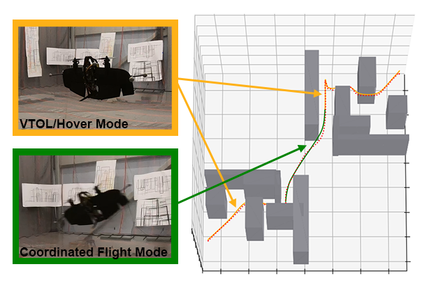
Figure 1: Multi-modal trajectory for a hybrid aircraft, which switches between hover mode and coordinated flight mode. The solid and dotted lines indicate the planned and real-life flight trajectories, respectively.

In this paper, we consider the motion planning problem for robotic vehicles with multi-modal dynamics. These vehicles switch between multiple modes that each exhibit dynamics governed by their own respective set of ordinary differential equations (ODEs). Mode transitions may occur due to deliberate (mechanical) configuration changes, e.g. in tiltrotor aircraft that switch between a vertical take-off and landing (VTOL) configuration and a more aerodynamically efficient cruise configuration [1]. Future urban mobility concepts may include vehicles that reduce travel time by combining driving and flying modes [2].

Motion planning for multi-modal dynamics has been extensively addressed using probabilistic sampling-based algorithms, such as Multi-Modal-PRM [3] or Random-MMP [4] which introduce mechanisms for sampling transitions between modes. However, having been developed with a focus on robotic manipulation problems involving contact, these planners do not address challenges posed by dynamics constraints. Sampling-based approaches like Sparse-RRT [5] can provide asymptotic optimality guarantees in planning for dynamics-constrained vehicles, but their reliance on randomly sampled control inputs leads to long planning times before solutions of acceptable quality are found even for low-dimensional single-mode systems. Therefore, we focus on optimization-based motion planning algorithms. These planners are generally only able to arrive at locally rather than globally optimal solutions, but algorithms such as CHOMP [6], STOMP [7], or GPMP [8] demonstrate an ability to rapidly arrive at high-quality solution paths. Timed Elastic Bands (TEBs) [9] perform trajectory optimization by representing trajectories using a factor graph. This enables the use of efficient graph optimization techniques, such as those developed for simultaneous localization and mapping applications [10]. Some TEB-based planners are indeed fast enough to function as a model predictive controller (MPC) [11].

Trajectory optimization approaches for multi-modal or hybrid systems often utilize a hierarchical architecture, combining local trajectory optimization with a higher-level planner to search over discrete actions. In order to be computationally tractable, such approaches may depend on simplified dynamics models [12] or learned approximations [13], which require significant engineering effort to design. Many resulting planners may be unsuitable for motion in tight, cluttered environments [14, 15]. Other approaches that do consider obstacles often require elaborate initialization schemes and are unable to converge without a high-quality initial guess [16].

We propose an algorithm for finding a locally time-optimal trajectory for multi-modal vehicles based on pose graph optimization. Our approach employs TEBs to obtain an intuitive and flexible transcription of dynamics, control input, and obstacle constraints in a sparse hypergraph. To enable application of TEBs to multi-modal motion planning, we introduce a composite pose graph structure that combines a sequence of pose graphs each corresponding to a single mode, as shown in Fig. 2. This allows discovery of optimized mode transition locations in cases where a mode sequence is known a priori. Additionally, we propose a scheme for generating an initial mode sequence and a mechanism for removal of unnecessary mode transitions to enable automatic discovery of optimized mode sequences.

Our work contains several contributions. Firstly, we present an efficient minimum-time motion planning algorithm for systems with multi-modal dynamics. Our planning framework optimizes the mode sequence, configuration space trajectory and control inputs, and incorporates obstacle avoidance. Secondly, we extend the TEB planning approach to enable planning with multi-modal dynamics. To achieve this, we introduce a composite pose graph structure that enables optimization of mode sequences. Finally, we present elaborate results that verify our algorithm in both simulation and real-world experiments. For the real-world experiments, we used a hybrid aircraft that can transition between VTOL mode with rotorcraft dynamics, and cruise mode with fixed-wing flight dynamics, as shown in Fig. 1.

The remainder of the paper is structured as follows. In Section II, we describe the multi-modal planning problem and provide a detailed overview of our algorithm. This is followed by experimental results in Section III, and finally conclusions in Section IV.

II MULTI-MODAL MOTION PLANNING ALGORITHM

We consider multi-modal vehicle dynamics described by a system of ordinary differential equations (ODEs), as follows:

$$\dot{x}(t)={f}_{M(t)}(x(t),{u}(t)),$$ (1)

where $x(t)$, ${u}(t)$, and $M(t)$ are respectively the state, control input, and dynamics mode as functions of time $t$. The minimum-time motion planning problem requires finding the fastest feasible trajectory from the start state ${x}_{\text{start}}$ to the goal state ${x}_{\text{goal}}$. In additional to dynamics constraints, it may involve state, control input and obstacle constraints, leading to the following optimization problem:

$$\min_{x(t),\;u(t),\;M(t)}\quad t_{e}$$ (2)

s.t. $${x}(0)={x}_{\text{start}},\;{x}(t_{e})={x}_{\text{goal}} \textrm{with}\;t_{e}\geq 0$$

$$\dot{x}(t)={f}_{M(t)}(x(t),{u}(t)) \forall t\in[0,t_{e}]$$

$$x(t)\in\mathcal{X}_{M(t)} \forall t\in[0,t_{e}]$$

$${{u}}(t)\in\mathcal{U}_{M(t)} \forall t\in[0,t_{e}]$$

$${{x}}(t)\notin\mathcal{X}^{obs}_{M(t)} \forall t\in[0,t_{e}]$$

where $\mathcal{X}_{M(t)}$ and $\mathcal{U}_{M(t)}$ are box-constrained state and control input sets corresponding to mode $M(t)$, respectively, and $\mathcal{X}^{obs}_{M(t)}$ is the corresponding set of obstacles in Euclidean space.

Our proposed algorithm for finding the solution to (2) is based on transforming the optimization problem into a sparse pose graph structure using the TEB approach. The pose graph captures the multi-modal state dynamics (1) using resizable trajectory segments. We use a probabilistic roadmap (PRM) planner to quickly obtain a trajectory used for initialization of the pose graph. The initial trajectory must be accompanied by an initial mode sequence $\Sigma_{\text{init}}$. As described in Section II-B, our proposed algorithm can find an optimal mode sequence through pruning under specific conditions. Mode pruning is performed at each iteration and followed by trajectory optimization, for which we represent the objective and constraints from (2) using penalty functions. This enables the use of efficient methods for unconstrained nonlinear least squares optimization. An overview of the complete algorithm is given in Algorithm 1, and individual steps are detailed in ensuing sections.

Algorithm 1 Multi-modal trajectory optimization

1:function Plan($x_{\text{start}},x_{\text{goal}},\Sigma_{\text{init}},N_{\text{iterations}}$)

2:     $P_{\text{init}}\leftarrow\text{ComputeInitialPath}(x_{\text{start}},x_{\text{goal}})$

3:     $B\leftarrow$InitializeTEBs$(P_{\text{init}},\Sigma_{\text{init}})$

4:     for $i\leftarrow 1$ to $N_{\text{iterations}}$ do

5:         for $m\leftarrow 1$ to $|B|$ do

6:              ResizeTEB$(B^{[m]})$

7:         end for

8:         PruneModes$(B)$

9:         Optimize$(B)$

10:     end for

11:     return ExtractTrajectory($B$)

12:end function

II-A Pose Graph Formulation

The vehicle state $x(t)$ may contain state variables governed by higher-order dynamics, e.g., second-order Newtonian dynamics. Consequently, $x(t)$ contains integrator states which we will not include in the pose graph. Hence, we eliminate integrator states from $x(t)$ and use the reduced pose vector $q(t)$ in the formulation of the pose graph. We realize that individual elements of $q(t)$ may be governed by dynamics of varying order, e.g., second-order vehicle dynamics combined with first-order control input servo dynamics, and will address this in the graph formulation.

We divide the trajectory $q(t)$ into single-mode segments and discretize these into individual poses. Each single-mode pose segment is captured in a pose graph, and the composite graph representing the entire trajectory $B$ is constructed by linking these pose graphs. A single-mode segment is described by a tuple, as follows:

$$B^{[m]}:=(Q^{[m]},U^{[m]},\Delta t^{[m]},M^{[m]}),$$ (3)

where $Q^{[m]}$, $U^{[m]}$ and $\Delta t^{[m]}$ are respectively the pose, control input and time step sequences, and $M^{[m]}$ is the segment mode. We denote the number of pose nodes in $B^{[m]}$ by $N^{[m]}$.

Penalty functions are used to capture the objective function and constraints in the pose graph, respectively. This structure enables formulation of the trajectory optimization problem as a nonlinear least squares program and the application of corresponding efficient solvers, as described in Section II-C. The resulting unconstrained objective function is given by

$$F(B) =\sum_{m=1}^{|B|}\sum_{i=1}^{N^{[m]}}\left(\alpha_{\text{o}}{e^{[m]}_{\text{o},i}}^{\top}e^{[m]}_{\text{o},i}+\sum_{\text{c}}\alpha_{\text{c}}{e^{[m]}_{\text{c},i}}^{\top}e^{[m]}_{\text{c},i}\right)$$ (4)

$$+\sum_{m=1}^{|B|-1}\alpha_{\text{t}}{e^{M^{[m]}\rightarrow M^{[m+1]}}_{t}}^{\top}e^{M^{[m]}\rightarrow M^{[m+1]}}_{t},$$

where $\alpha$ are weights corresponding to the objective and constraint penalty functions ($e^{[m]}_{\text{o},i}$ and $e^{[m]}_{\text{c},i}$), which are defined in Table I. In this table, a system of ODEs governing $q$ is denoted with $g$, and its order is denoted with $n$. Similarly, control inputs $u$ (with corresponding integrator states) are governed by $h$. As $x$ may contain integrator states, the state constraint $x\in\mathcal{X}$ and control input constraint $u\in\mathcal{U}$ can technically apply to $q$ and $u$ and their derivatives up to $q^{(n-1)}$ and $u^{(n-1)}$. If this is the case, additional functions $g$ and $h$, each with varying order, may be defined according to the form given for Vehicle Dynamics in Table I. The resulting value of the penalty $e_{c}$ for the dynamics is proportional to the difference between the output of the nominal dynamics given by given by $g$ or $h$, and the configuration derivative (e.g., $q^{(n)}$) obtained from the current pose graph.

State derivatives are obtained using the finite difference method, as reflected by the sequence of connected nodes. The start and goal states are directly substituted into constant first and final pose nodes and thus enforced through the dynamics constraint. Similarly to the state constraint $x\in\mathcal{X}$, $x_{\text{start}}$ and $x_{\text{goal}}$ may constrain the initial and final velocities, accelerations, and higher derivatives up to order $n-1$. Consequently, these boundary constraints may require substitution into vehicle dynamics penalty terms connected to the first and final $n$ poses. Obstacles are defined in the Euclidean space and thus only pertain to $q$ itself, so that the Euclidean distance to the closest obstacle can be taken as ObstacleDistance. Finally, the penalty functions $e^{M^{[m]}\rightarrow M^{[m+1]}}_{t}$ impose continuity constraints at the mode transitions.

TABLE I: Transformation of trajectory optimization objective and constraints to pose graph.

Objective/Constraint		Penalty Term ($e^{[m]}_{\text{o},i}$ or $e^{[m]}_{\text{c},i}$)	Connected Nodes
Time Minimization	$\min t_{e}$	$\Delta t_{i}$	$\Delta t_{i}$
Start and Goal States	${x}(0)={x}_{\text{start}},\;{x}(t_{e})={x}_{\text{goal}}$	Substitution into first and final pose nodes.
Vehicle Dynamics	$\dot{x}(t)={f}_{M(t)}(x(t),{u}(t))$	$|q^{(n)}_{i}-{g}_{M^{[m]}}(q_{i},\dots,q^{(n-1)}_{i},{u}_{i})|$ $|u^{(n)}_{i}-{h}_{M^{[m]}}(u_{i},\dots,u^{(n-1)}_{i})|$	$q_{i-\lfloor\frac{n}{2}\rfloor},\dots,q_{i+\lceil\frac{n}{2}\rceil},\Delta t_{i-\lfloor\frac{n}{2}\rfloor},\dots,\Delta t_{i+\lfloor\frac{n}{2}\rfloor},u_{i}$ $u_{i-\lfloor\frac{n}{2}\rfloor},\dots,u_{i+\lceil\frac{n}{2}\rceil},\Delta t_{i-\lfloor\frac{n}{2}\rfloor},\dots,\Delta t_{i+\lfloor\frac{n}{2}\rfloor}$
State Feasibility	$x(t)\in\mathcal{X}_{M(t)}$	$\max(0,q_{i}-q^{\text{max}}_{M^{[m]}})+\max(0,q^{\text{min}}_{M^{[m]}}-q_{i})$	$q_{i}$
Control Input Feasibility	${{u}}(t)\in\mathcal{U}_{M(t)}$	$\max(0,u_{i}-u^{\text{max}}_{M^{[m]}})+\max(0,u^{\text{min}}_{M^{[m]}}-u_{i})$	$u_{i}$
Obstacle Avoidance	${{x}}(t)\notin\mathcal{X}^{obs}_{M(t)}$	$\max(0,-\text{ObstacleDistance}(M(t),q_{i}))$	$q_{i}$

$F(B)$ depends only sparsely on the elements of the trajectory $B$. Represented as a hypergraph, each $q_{i}$, $u_{i}$ and $\Delta T_{i}$ are taken to be the vertices, connected by edges corresponding to the various penalty functions. Fig. 2 illustrates this graph as well as its sparse, periodic structure. Finding the optimal trajectory $B^{\star}$ then amounts to solving the following unconstrained nonlinear least squares program

$$B^{\star}=\operatorname*{arg\,min}_{B}{F(B)}.$$ (5)

We found that assigning the weights $\alpha_{c}$, $\alpha_{t}$ and $\alpha_{o}$ such that the minimum-time objective does not compete with minimization of dynamics residuals or obstacle avoidance (i.e., $\alpha_{t}\approx\alpha_{c}\gg\alpha_{o}$) gives favorable results. With such a weight assignment, the optimization is initially guided towards satisfying dynamic feasibility and obstacle constraints. Once residuals corresponding to these constraints have been minimized significantly, the time minimization cost (with lower weight) becomes a significant contributor to the overall cost function, guiding the optimization towards lower time solutions.

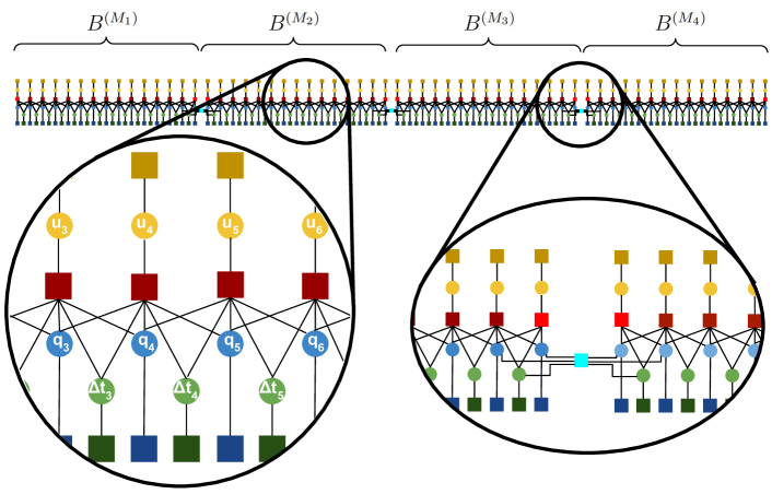
Figure 2: Factor graph representation of the cost of a four-mode trajectory $B=[B^{[M_{1}]},B^{[M_{2}]},B^{[M_{3}]},B^{[M_{4}]}]$. Round nodes represent vertices containing optimizable parameters, squares with links represent edges of the factor graph and are colored according to the class of their corresponding cost function (red: second order dynamics, blue: obstacle avoidance, yellow: control input limit, green: time minimization, cyan: mode transition).

II-B Initialization

An initial trajectory with corresponding mode sequence is required to construct and initialize the factor graph. We found the algorithm to be generally insensitive to state and control input feasibility and time-optimality of the initial trajectory, but somewhat sensitive to satisfaction of the obstacle avoidance constraint. Hence, we opt for a sampling-based planner on $\mathbf{SE}(3)$, specifically PRM*, to quickly obtain a collision-free initial trajectory [17]. The required mapping from $\mathbf{SE}(3)$ to the state $q$ is trivial for most vehicle dynamics applications, and linear and spherical linear interpolation (Slerp) are used to obtain continuous position and orientation between PRM* waypoints. Time differences are initialized to a small positive value, and control inputs are initialized to the mean of their bounds. As shown in Section III, the algorithm obtains reliable convergence despite the infeasibility of the initial trajectories.

The initial mode sequence may be based on engineering knowledge of the system and scenario. Additionally, if the vehicle mode transition graph is fully connected, our algorithm is able to arrive at any subsequence of the initial mode sequence through mode pruning. Hence, it is able to find an optimal transition sequence after initialization with a sequence that repeatedly loops through all modes. Suppose we expect at most $N_{\text{transitions}}$ transitions are required between modes $M_{1},\ldots,M_{N_{\text{m}}}$, then such a looping mode sequence is constructed as

$$\Sigma=[\underbrace{M_{1},\dots,M_{N_{\text{m}}}}_{1},\dots,\underbrace{M_{1},\dots,M_{N_{\text{m}}}}_{N_{\text{transitions}}}].$$

The initial geometric trajectory is then divided in single-mode segments of equal length. After initialization, redundant and unnecessary modes are incrementally eliminated during the trajectory optimization process, as shown in Fig. 3. The complexity of this method scales linearly with the number of modes and transitions, and thus it enables our algorithm to avoid the combinatorial explosion from which mode sequencers may suffer. We verified its favorable scaling in systems with a limited number of modes, but expect it to be impractical for systems with a very large number of modes, which require an excessive initial mode sequence.

II-C Graph Optimization

As given by (5), the motion planning process is formulated as an unconstrained minimization of the cost function $F(B)$. We chose the Levenberg-Marquardt (LM) algorithm [18] to solve this nonlinear least squares problem. For notational simplicity, we will limit the description in this section to a single-mode trajectory, i.e., $|B|=1$. There is no fundamental difference between this and multi-modal cases.

Starting at an initial guess, LM iteratively linearizes around $B$ and finds an increment $\Delta\mathbf{x}$ to be applied to the trajectory. This increment is represented as a vector containing the increments $\Delta q_{i}$, $\Delta u_{i}$ and $\Delta\Delta T_{i}$, which are applied as follows:

$$B\mathbin{\mathop{\boxplus}}\Delta\mathbf{x} =(Q\mathbin{\mathop{\boxplus}}\Delta Q,U\mathbin{\mathop{\boxplus}}\Delta U,\tau\mathbin{\mathop{\boxplus}}\Delta\tau)$$ (6)

$$Q\mathbin{\mathop{\boxplus}}\Delta Q =\{q_{i}\mathbin{\mathop{\boxplus}}\Delta q_{i}\}_{i=0\ldots N}$$ (7)

$$U\mathbin{\mathop{\boxplus}}\Delta U =\{u_{i}\mathbin{\mathop{\boxplus}}\Delta u_{i}\}_{i=0\ldots N}$$ (8)

$$\tau\mathbin{\mathop{\boxplus}}\Delta\tau =\{\Delta T_{i}+\Delta\Delta T_{i}\}_{i=0\ldots N-1}$$ (9)

We use the $\mathbin{\mathop{\boxplus}}$ operator to denote the element-wise application of the increments. When using $\mathbin{\mathop{\boxplus}}$ to apply increments to $q_{i}$ or $u_{i}$, its exact behavior depends on the representation of the increments, configurations, and control inputs. For example, for some of the scenarios described in Section III, the configurations $q_{i}$ are taken to be poses in SE(3) with the rotation stored as a quaternion, but the increments $\Delta q_{i}$ contain the rotational increment in a non-overparametrized representation (the axis of a normalized quaternion), since small increments are far from the singularities encountered in such a representation. Hence, the $\mathbin{\mathop{\boxplus}}$ operator behaves like motion composition in this case [19].

Using a first-order approximation for the cost terms ${e}_{c,i}(B^{[m]}\mathbin{\mathop{\boxplus}}\Delta\mathbf{x})\approx{e}_{c,i}(B^{[m]})+{J}_{c,i}\Delta\mathbf{x}$ with ${J}_{c,i}$ the Jacobian of the penalty function, we obtain approximations of the cost after increment per penalty $c$ and pose index $i$ as

$$F {}_{c,i}(B\mathbin{\mathop{\boxplus}}\Delta\mathbf{x})$$

$$= ~{}\alpha_{c}{e}_{c,i}(B\mathbin{\mathop{\boxplus}}\Delta{x})^{\top}{e}_{c,i}(B\mathbin{\mathop{\boxplus}}\Delta\mathbf{x})$$ (10)

$$\approx ~{}\alpha_{c}({e}_{c,i}(B)+{J}_{c,i}\Delta\mathbf{x})^{\top}({e}_{c,i}(B)+{J}_{c,i}\Delta\mathbf{x})$$

$$= ~{}\alpha_{c}(\underbrace{{e}_{c,i}(B)^{\top}{e}_{c,i}(B)}_{c_{c,i}/\alpha_{c}}+2\underbrace{{e}_{c,i}(B)^{\top}{J}_{c,i}}_{{{b}_{c,i}}^{\top}/\alpha_{c}}\Delta\mathbf{x}+\Delta\mathbf{x}^{\top}\underbrace{{{J}_{c,i}}^{\top}{J}_{c,i}}_{{H}_{c,i}/\alpha_{c}}\Delta\mathbf{x})$$

A similar form is obtained for the objective cost, so that

$$F (B\mathbin{\mathop{\boxplus}}\Delta\mathbf{x})$$

$$\approx\sum_{c,i}c_{c,i}+2{{b}_{c,i}}^{\top}\Delta\mathbf{x}+\Delta\mathbf{x}^{\top}{H}_{c,i}\Delta\mathbf{x}$$ (11)

$$+\sum_{i}c_{o,i}+2{{b}_{o,i}}^{\top}\Delta\mathbf{x}+\Delta\mathbf{x}^{\top}{H}_{o,i}\Delta\mathbf{x}$$

$$=c+2{b}^{\top}\Delta\mathbf{x}+\Delta\mathbf{x}^{\top}{H}\Delta\mathbf{x}$$

Next, the increment $\Delta\mathbf{x}^{\star}$ is obtained by solving

$$({H}+\lambda{I})\Delta\mathbf{x}^{\star}=-{b},$$ (12)

where $\lambda$ is the damping factor. At $\lambda=0$, the Gauss-Newton algorithm is recovered. However, to better handle nonlinear costs, LM adaptively sets $\lambda$ to control the maximum size of the increments $\Delta\mathbf{x}^{\star}$.

Due to the structure of the cost function and its representation as factor graph shown in Fig. 2, each of the individual Jacobians $J_{c,i}$ only depends on very few elements of $B$ and $\Delta\mathbf{x}$, leading to sparsity of ${H}$. The $\mathrm{g}^{2}\mathrm{o}$ library [20] was chosen for implementation of the motion planner, as it allows specification of the cost function as a graph, and can thus exploit its sparse structure to efficiently perform the optimization.

II-D Incremental Trajectory Resizing

The shape and time of the trajectory may significantly change during optimization, leading to changing position and time differences between consecutive poses. Hence, it is necessary to insert and delete poses in order to maintain efficiency, and accurate finite-differencing and obstacle avoidance.

Position-based removal ensures that resolution is always sufficient for satisfactory obstacle avoidance. Given distance thresholds $d_{min}$ and $d_{max}$ and a function $\mathrm{Position}(q_{i})$ that maps the pose to a point in Euclidean space, a pose $q_{i}$ (with corresponding control input and time difference) is removed if $\left|\mathrm{Position}(q_{i})-\mathrm{Position}(q_{i+1})\right|<d_{min}$. The new time difference $\Delta T_{i}$ (previously $\Delta T_{i+1}$) is incremented by the removed time difference to maintain identical trajectory time.

When $\left|\mathrm{Position}(q_{i})-\mathrm{Position}(q_{i+1})\right|>d_{max}$, a new pose is inserted between $q_{i}$ and $q_{i+1}$. The newly inserted pose $q_{i+1}$ and control input $u_{i+1}$ are computed using system-dependent interpolation functions $q_{i+1}=\mathrm{Interp}_{q}(q_{i},q_{i+2},0.5)$ and $u_{i+1}=\mathrm{Interp}_{u}(u_{i},u_{i+2},0.5)$. In typical vehicle motion planning scenarios, $q_{i}$ represents poses in SE(3), such that $\mathrm{Interp}_{q}$ performs linear interpolation for the translational part of the pose, and Slerp for the rotational component. For the vector-valued control inputs $u_{i}$, $\mathrm{Interp}_{u}$ performs linear interpolation. Time-differences are each set to half of the previous time difference.

An analogous procedure is used for time-difference based adjustments. Here, $\Delta T_{min}$ and $\Delta T_{max}$ trigger removal or insertion of poses in order to maintain a time-resolution adequate for good fidelity of the dynamics model.

II-E Mode pruning

The resizing process described in Section II-D often leads to expansion or shrinkage of the single-mode trajectories that compose the full multi-modal trajectory. This process can result in trajectories being iteratively shrunk until only their first and last poses remain. To fully eliminate such a trajectory segment $B^{[n]}$, our algorithm prunes them from the factor graph by deleting any remaining poses and adding the relevant transition constraints between the adjacent trajectories $B^{[n-1]}$ and $B^{[n+1]}$. If the trajectories $B^{[n-1]}$ and $B^{[n+1]}$ correspond to the same mode, they are combined into a single trajectory instead of being joined by a transition constraint. This process allows discovery of an optimized mode sequence in cases where the initialization contains unnecessary mode switches, as illustrated in Fig. 3.

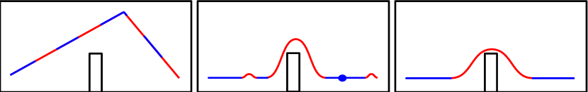
Figure 3: Pruning of modes of which the trajectories were eliminated through the resizing process, and merging of trajectories of the same mode that become adjacent due to pruning of intermediate modes. The left graphic shows an initial guess for a multi-modal trajectory, with colors representing separate modes. The middle graphic illustrates the partially optimized trajectory in which the third trajectory of the red mode has been resized away. The right graphic shows the fully optimized trajectory after pruning and merging.

III EXPERIMENTAL RESULTS

We now construct motion planners for a variety of single-mode and multi-modal systems to experimentally demonstrate our approach. All experiments were executed single-threaded on an Intel Core i7 2600k CPU, and Jacobians were computed numerically. A video of the experiments is available at https://youtu.be/XdUtyGu3p1o.

III-A Dubins Car

To illustrate the effectiveness of our dynamics transcription approach, we first consider a simple single-mode Dubins car. Graph-based planning for a Dubins car is also demonstrated by [9], but their proposed method requires hand-designed constraints based on path geometry. Our systematic transcription of the dynamics results in a different pose graph formulation. In particular, we consider a car model with bounded control inputs for acceleration $a_{\text{des}}$ and steering angle $\alpha$. Fig. 4 shows planning results and a comparison of our proposed algorithm with RRT* [17]. The RRT* steering function is based on Dubins geometry with turning radius equivalent to that of the model used in our planner at the saturated steering angle.

(a) Optimized trajectory using FGO approach alongside RRT* solutions.

(b) Control inputs $\alpha_{i}$ and $a_{\text{des},i}$ along the FGO solution trajectory.

Planner	Time [s]	Path length
FGO	3.5	51.176
RRT*	6	56.705
RRT*	500	53.406
RRT*	1500	52.577

(c) Runtime comparison

Figure 4: Trajectory planning for the Dubins car vehicle using our factor graph optimization based planner (FGO) and RRT*. Fig. 4(a) shows result trajectories color coded corresponding to the entries in Fig. 4(c), which lists planning times for each result (FGO result includes PRM-based initialization, which requires $<0.1$ seconds). Note that the FGO optimization recovers control inputs which resemble the optimal bang-bang policy (Fig. 4(b)).

When starting from an low-quality, potentially dynamically infeasible, initial trajectory, our proposed planner may take several seconds to converge, as shown in Fig. 4(c). We observed that this convergence time is strongly reduced if a high-quality initial trajectory is available, such as when performing replanning to incorporate changed start and goal states, or small variations in the obstacle map. The capability to efficiently utilize previous solutions, gives our algorithm potential for online applications where the planned trajectory must be continuously updated.

III-B Airplane

We plan trajectories for an airplane which can both fly and taxi on the ground. This multi-modal system is described by the same dynamics as the Dubins car for the taxi mode, and uses a point-mass aircraft model in the flight mode. The flight mode represents the pose of the airplane using $(x,y,z)$ for the position, pitch angle $\theta$ and heading angle $\psi$. The control input is given by the thrust, relative lift coefficient and a roll angle. The flight mode dynamics include a second-order lift and drag force model [21]. When transitioning from taxi to flight, a mode transition constraint ensures continuity in the velocity as well as pitch and yaw angle.

Fig. 5 shows an optimized trajectory for this multi-modal system. In the example, the taxi mode is preferred, such that the vehicle stays on the ground for as long as possible, only taking off to fly over an obstacle and reach the goal which is not accessible in taxi mode. This is achieved by replacing the original time-optimality cost with an energy consumption cost. Energy consumption is modelled by assigning a fixed power usage to each mode, with the power required by the flight mode set to be significantly higher than that of the taxi mode. Since this modification is equivalent to assigning the time-optimality cost for the flight mode to be higher than that of the taxi mode by a constant multiplier, this energy consumption cost is straightforward to model within our framework.

(a) Trajectory (blue) and initial guess (red).

(b) Trajectory in XY plane.

(c) Trajectory in XZ plane.

(d) Cost during optimization.

Figure 5: Trajectory optimization for a taxiing and flying airplane. Transition from taxi mode to flight mode is indicated by cross markers.

III-C Tailsitter

To examine the planner’s performance in optimizing trajectories for more realistic vehicle dynamics, we implement the $\phi$-theory model presented in [22]. This model describes the dynamics of a tailsitter VTOL aircraft including post-stall behavior using polynomial equations. It provides 6 degree-of-freedom equations of motion as a second order ODE, with four control inputs $\omega_{L}$, $\omega_{R}$, $\delta_{L}$ and $\delta_{R}$ which correspond to left and right propeller angular velocities, and left and right elevon deflections, respectively. Fig. 6 shows an example trajectory planned for this model, as well as results from flying the trajectory with the tailsitter aircraft described in [23]. In the flight experiments, we used the planned position, velocity, acceleration, attitude and angular rate as reference for the on-board flight controller. The consistency between planned and real-life trajectories demonstrates the applicability of our planning algorithm to complicated models that realistically capture complex dynamics using an increased number of state variables.

(a) Planned (blue) and flown (red) tailsitter trajectories.

(b) Planned control inputs along the trajectory.

Figure 6: Optimized trajectory of 329 poses for tailsitter using $\phi$-theory model. Convergence time was 10 seconds.

III-D Multi-Modal Tailsitter

As demonstrated above, our planner is able use the $\phi$-theory tailsitter model to create high quality trajectories incorporating transitions between hover and level flight. However, using such a global description of the vehicle dynamics may lead to optimized paths that are undesirable due to restrictions in the control scheme on the vehicle. For example, planned paths might contain sideways “knife-edge” flight which is difficult for a controller to steadily track. Therefore, it is useful to consider a planner which treats the tailsitter as a multi-modal vehicle capable of transitioning between a multicopter-like hover and a coordinated flight modes. Fig. 1 shows planning and real-life flight results for multi-modal trajectories planned using the airplane model from Section III-B to describe coordinated flight, and a simple multicopter model with a two-dimensional control input consisting of pitch and roll angles to describe hover.

IV CONCLUSION

Our algorithm addresses the motion planning problem for multi-modal vehicle dynamics using a pose graph formulation. Leveraging efficient pose graph optimization algorithms, it is able to produce trajectories for a wide variety of vehicles. We verify its performance and applicability through extensive computational experiments and real-life experiments using a VTOL aircraft. While the algorithm does not guarantee discovery of an optimal mode sequence without an appropriate initialization, it does demonstrate the ability to rapidly approach optimal trajectories and mode sequences in a variety of realistic scenarios.

References

- [1] C. Papachristos, K. Alexis, and A. Tzes, “Design and experimental attitude control of an unmanned tilt-rotor aerial vehicle,” in 2011 15th International Conference on Advanced Robotics (ICAR), 2011, pp. 465–470.
- [2] A. R. Kadhiresan and M. J. Duffy, “Conceptual design and mission analysis for eVTOL urban air mobility flight vehicle configurations,” in AIAA Aviation 2019 Forum. American Institute of Aeronautics and Astronautics, Jun. 2019. [Online]. Available: https://doi.org/10.2514/6.2019-2873
- [3] K. Hauser and J.-C. Latombe, “Multi-modal motion planning in non-expansive spaces,” Springer Tracts in Advanced Robotics Algorithmic Foundation of Robotics VIII, p. 615–630, 2009.
- [4] K. Hauser and V. Ng-Thow-Hing, “Randomized multi-modal motion planning for a humanoid robot manipulation task,” The International Journal of Robotics Research, vol. 30, no. 6, pp. 678–698, Dec. 2010. [Online]. Available: https://doi.org/10.1177/0278364910386985
- [5] Z. Littlefield, Y. Li, and K. E. Bekris, “Efficient sampling-based motion planning with asymptotic near-optimality guarantees for systems with dynamics,” 2013 IEEE/RSJ International Conference on Intelligent Robots and Systems, 2013.
- [6] N. Ratliff, M. Zucker, J. A. Bagnell, and S. Srinivasa, “CHOMP: Gradient optimization techniques for efficient motion planning,” in 2009 IEEE International Conference on Robotics and Automation. IEEE, May 2009. [Online]. Available: https://doi.org/10.1109/robot.2009.5152817
- [7] M. Kalakrishnan, S. Chitta, E. Theodorou, P. Pastor, and S. Schaal, “STOMP: Stochastic trajectory optimization for motion planning,” in 2011 IEEE International Conference on Robotics and Automation. IEEE, May 2011. [Online]. Available: https://doi.org/10.1109/icra.2011.5980280
- [8] M. Mukadam, J. Dong, X. Yan, F. Dellaert, and B. Boots, “Continuous-time gaussian process motion planning via probabilistic inference,” The International Journal of Robotics Research, vol. 37, no. 11, pp. 1319–1340, Sep. 2018. [Online]. Available: https://doi.org/10.1177/0278364918790369
- [9] C. Rösmann, W. Feiten, T. Wösch, F. Hoffmann, and T. Bertram, “Trajectory modification considering dynamic constraints of autonomous robots,” Proc. 7th German Conference on Robotics, Munich, Germany, p. 74–79, 2012.
- [10] F. Dellaert and M. Kaess, “Factor graphs for robot perception,” Foundations and Trends in Robotics, vol. 6, no. 1-2, pp. 1–139, 2017. [Online]. Available: https://doi.org/10.1561/2300000043
- [11] C. Rösmann, F. Hoffmann, and T. Bertram, “Timed-elastic-bands for time-optimal point-to-point nonlinear model predictive control,” in 2015 European Control Conference (ECC), 2015, pp. 3352–3357.
- [12] E. Fernandez-Gonzalez, B. Williams, and E. Karpas, “ScottyActivity: Mixed discrete-continuous planning with convex optimization,” Journal of Artificial Intelligence Research, vol. 62, pp. 579–664, Jul. 2018. [Online]. Available: https://doi.org/10.1613/jair.1.11219
- [13] H. Suh, X. Xiong, A. Singletary, A. D. Ames, and J. W. Burdick, “Energy-efficient motion planning for multi-modal hybrid locomotion,” in 2020 IEEE/RSJ International Conference on Intelligent Robots and Systems (IROS). IEEE, 2020. [Online]. Available: http://ames.caltech.edu/suh2020optimal.pdf
- [14] H. Saranathan and M. J. Grant, “Relaxed autonomously switched hybrid system approach to indirect multiphase aerospace trajectory optimization,” Journal of Spacecraft and Rockets, vol. 55, no. 3, pp. 611–621, May 2018. [Online]. Available: https://doi.org/10.2514/1.a34012
- [15] J. Pajarinen, V. Kyrki, M. Koval, S. Srinivasa, J. Peters, and G. Neumann, “Hybrid control trajectory optimization under uncertainty,” in 2017 IEEE/RSJ International Conference on Intelligent Robots and Systems (IROS). IEEE, Sep. 2017. [Online]. Available: https://doi.org/10.1109/iros.2017.8206460
- [16] S. Choudhury, Y. Hou, G. Lee, and S. S. Srinivasa, “Hybrid DDP in clutter (CHDDP): trajectory optimization for hybrid dynamical system in cluttered environments,” CoRR, vol. abs/1710.05231, 2017. [Online]. Available: http://arxiv.org/abs/1710.05231
- [17] S. Karaman and E. Frazzoli, “Sampling-based algorithms for optimal motion planning,” The International Journal of Robotics Research, vol. 30, no. 7, pp. 846–894, Jun. 2011. [Online]. Available: https://doi.org/10.1177/0278364911406761
- [18] J. J. Moré, “The levenberg-marquardt algorithm: Implementation and theory,” in Lecture Notes in Mathematics. Springer Berlin Heidelberg, 1978, pp. 105–116. [Online]. Available: https://doi.org/10.1007/bfb0067700
- [19] C. Hertzberg, R. Wagner, U. Frese, and L. Schröder, “Integrating generic sensor fusion algorithms with sound state representations through encapsulation of manifolds,” Information Fusion, vol. 14, no. 1, pp. 57–77, Jan. 2013. [Online]. Available: https://doi.org/10.1016/j.inffus.2011.08.003
- [20] R. Kummerle, G. Grisetti, H. Strasdat, K. Konolige, and W. Burgard, “G2o: A general framework for graph optimization,” 2011 IEEE International Conference on Robotics and Automation, 2011.
- [21] L. A. Weitz, “Derivation of a point-mass aircraft model used for fast-time simulation,” The MITRE Corporation, Tech. Rep., 2015.
- [22] L. R. Lustosa, F. Defaÿ, and J.-M. Moschetta, “Global singularity-free aerodynamic model for algorithmic flight control of tail sitters,” Journal of Guidance, Control, and Dynamics, vol. 42, no. 2, pp. 303–316, Feb. 2019. [Online]. Available: https://doi.org/10.2514/1.g003374
- [23] M. Bronz, E. Tal, F. Favalli, and S. Karaman, “Mission-oriented additive manufacturing of modular mini-UAVs,” in AIAA Scitech 2020 Forum, 2020. [Online]. Available: https://arc.aiaa.org/doi/abs/10.2514/6.2020-0064