An Inverse QSAR Method Based on Linear Regression and Integer Programming

Jianshen Zhu¹, Naveed Ahmed Azam¹, Kazuya Haraguchi¹, Liang Zhao², Hiroshi Nagamochi¹ and Tatsuya Akutsu³

1. Department of Applied Mathematics and Physics, Kyoto University, Kyoto 606-8501, Japan
2. Graduate School of Advanced Integrated Studies in Human Survavibility (Shishu-Kan), Kyoto University, Kyoto 606-8306, Japan
3. Bioinformatics Center, Institute for Chemical Research, Kyoto University, Uji 611-0011, Japan

Abstract
Recently a novel framework has been proposed for designing the molecular structure of chemical compounds using both artificial neural networks (ANNs) and mixed integer linear programming (MILP). In the framework, we first define a feature vector $f(\mathbb{C})$ of a chemical graph $\mathbb{C}$ and construct an ANN that maps $x=f(\mathbb{C})$ to a predicted value $\eta(x)$ of a chemical property $\pi$ to $\mathbb{C}$. After this, we formulate an MILP that simulates the computation process of $f(\mathbb{C})$ from $\mathbb{C}$ and that of $\eta(x)$ from $x$. Given a target value $y^{*}$ of the chemical property $\pi$, we infer a chemical graph $\mathbb{C}^{\dagger}$ such that $\eta(f(\mathbb{C}^{\dagger}))=y^{*}$ by solving the MILP. In this paper, we use linear regression to construct a prediction function $\eta$ instead of ANNs. For this, we derive an MILP formulation that simulates the computation process of a prediction function by linear regression. The results of computational experiments suggest our method can infer chemical graphs with around up to 50 non-hydrogen atoms.

Keywords: Machine Learning, Linear Regression, Integer Programming, Cheminformatics, Materials Informatics, QSAR/QSPR, Molecular Design.

1 Introduction

Background  Analysis of chemical compounds is one of the important applications of intelligent computing. Indeed, various machine learning methods have been applied to the prediction of chemical activities from their structural data, where such a problem is often referred to as quantitative structure activity relationship (QSAR) [1, 2]. Recently, neural networks and deep-learning technologies have extensively been applied to QSAR [3].

In addition to QSAR, extensive studies have been done on inverse quantitative structure activity relationship (inverse QSAR), which seeks for chemical structures having desired chemical activities under some constraints. Since it is difficult to directly handle chemical structures in both QSAR and inverse QSAR, chemical compounds are usually represented as vectors of real or integer numbers, which are often called descriptors in chemoinformatics and correspond to feature vectors in machine learning. One major approach in inverse QSAR is to infer feature vectors from given chemical activities and constraints and then reconstruct chemical structures from these feature vectors [4, 5, 6], where chemical structures are usually treated as undirected graphs. However, the reconstruction itself is a challenging task because the number of possible chemical graphs is huge. For example, chemical graphs with up to 30 atoms (vertices) C, N, O, and S may exceed $10^{60}$ [7]. Indeed, it is NP-hard to infer a chemical graph from a given feature vector except for some simple cases [8]. Due to this inherent difficulty, most existing methods for inverse QSAR do not guarantee optimal or exact solutions.

As a new approach, extensive studies have recently been done for inverse QSAR using artificial neural networks (ANNs), especially using graph convolutional networks [9]. For example, recurrent neural networks [11, 12], variational autoencoders [10], grammar variational autoencoders [13], generative adversarial networks [14], and invertible flow models [15, 16] have been applied. However, these methods do not yet guarantee optimal or exact solutions.

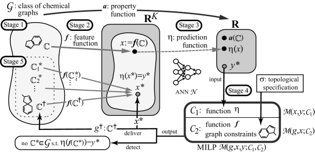
Figure 1: An illustration of a framework for inferring a set of chemical graphs $\mathbb{C}^{*}$.

Framework  Akutsu and Nagamochi [17] proved that the computation process of a given ANN can be simulated with a mixed integer linear programming (MILP). Based on this, a novel framework for inferring chemical graphs has been developed [18, 19], as illustrated in Figure 1. It constructs a prediction function in the first phase and infers a chemical graph in the second phase. The first phase of the framework consists of three stages. In Stage 1, we choose a chemical property $\pi$ and a class $\mathcal{G}$ of graphs, where a property function $a$ is defined so that $a(\mathbb{C})$ is the value of $\pi$ for a compound $\mathbb{C}\in\mathcal{G}$, and collect a data set $D_{\pi}$ of chemical graphs in $\mathcal{G}$ such that $a(\mathbb{C})$ is available for every $\mathbb{C}\in D_{\pi}$. In Stage 2, we introduce a feature function $f:\mathcal{G}\to\mathbb{R}^{K}$ for a positive integer $K$. In Stage 3, we construct a prediction function $\eta$ with an ANN $\mathcal{N}$ that, given a vector $x\in\mathbb{R}^{K}$, returns a value $y=\eta(x)\in\mathbb{R}$ so that $\eta(f(\mathbb{C}))$ serves as a predicted value to the real value $a(\mathbb{C})$ of $\pi$ for each $\mathbb{C}\in D_{\pi}$. Given a target chemical value $y^{*}$, the second phase infers chemical graphs $\mathbb{C}^{*}$ with $\eta(f(\mathbb{C}^{*}))=y^{*}$ in the next two stages. We have obtained a feature function $f$ and a prediction function $\eta$ and call an additional constraint on the substructures of target chemical graphs a topological specification. In Stage 4, we prepare the following two MILP formulations:

1. MILP $\mathcal{M}(x,y;\mathcal{C}_{1})$ with a set $\mathcal{C}_{1}$ of linear constraints on variables $x$ and $y$ (and some other auxiliary variables) simulates the process of computing $y:=\eta(x)$ from a vector $x$; and

2. MILP $\mathcal{M}(g,x;\mathcal{C}_{2})$ with a set $\mathcal{C}_{2}$ of linear constraints on variable $x$ and a variable vector $g$ that represents a chemical graph $\mathbb{C}$ (and some other auxiliary variables) simulates the process of computing $x:=f(\mathbb{C})$ from a chemical graph $\mathbb{C}$ and chooses a chemical graph $\mathbb{C}$ that satisfies the given topological specification $\sigma$.

Given a target value $y^{*}\in\mathbb{R}$, we solve the combined MILP $\mathcal{M}(g,x,y;\mathcal{C}_{1},\mathcal{C}_{2})$ to find a feature vector $x^{*}\in\mathbb{R}^{K}$ and a chemical graph $\mathbb{C}^{\dagger}$ with the specification $\sigma$ such that $f(\mathbb{C}^{\dagger})=x^{*}$ and $\eta(x^{*})=y^{*}$ (where if the MILP instance is infeasible then this suggests that there does not exist such a desired chemical graph). In Stage 5, we generate other chemical graphs $\mathbb{C}^{*}$ such that $\eta(f(\mathbb{C}^{*}))=y^{*}$ based on the output chemical graph $\mathbb{C}^{\dagger}$.

MILP formulations required in Stage 4 have been designed for chemical compounds with cycle index 0 (i.e., acyclic) [19, 20], cycle index 1 [21] and cycle index 2 [22], where no sophisticated topological specification was available yet. Azam et al. [20] introduced a restricted class of acyclic graphs that is characterized by an integer ${\rho}$, called a “branch-parameter” such that the restricted class still covers most of the acyclic chemical compounds in the database. Akutsu and Nagamochi [23] extended the idea to define a restricted class of cyclic graphs, called “${\rho}$-lean cyclic graphs” and introduced a set of flexible rules for describing a topological specification. Recently, Tanaka et al. [26] used a decision tree to construct a prediction function $\eta$ in Stage 3 in the framework and derived an MILP $\mathcal{M}(x,y;\mathcal{C}_{1})$ that simulates the computation process of a decision tree.

Two-layered Model  Recently Shi et al. [25] proposed a new model, called a two-layered model for representing the feature of a chemical graph in order to deal with an arbitrary graph in the framework and refined the set of rules for describing a topological specification so that a prescribed structure can be included in both of the acyclic and cyclic parts of $\mathbb{C}$. In the two-layered model, a chemical graph $\mathbb{C}$ with a parameter ${\rho}\geq 1$ is regarded as two parts: the exterior and the interior of the hydrogen-suppressed chemical graph $\langle\mathbb{C}\rangle$ obtained from $\mathbb{C}$ by removing hydrogen. The exterior consists of maximal acyclic induced subgraphs with height at most ${\rho}$ in $\langle\mathbb{C}\rangle$ and the interior is the connected subgraph of $\langle\mathbb{C}\rangle$ obtained by ignoring the exterior. Shi et al. [25] defined a feature vector $f(\mathbb{C})$ of a chemical graph $\mathbb{C}$ to be a combination of the frequency of adjacent atom pairs in the interior and the frequency of chemical acyclic graphs among the set of chemical rooted trees $T_{u}$ rooted at interior-vertices $u$. Recently, Tanaka et al. [26] extend the model to treat a chemical graph with hydrogens directly so that more variety of chemical rooted trees represent the feature of the exterior.

Contribution  In this paper, we first make a slight modification to a model of chemical graphs proposed by Tanaka et al. [26] so that we can treat a chemical element with multi-valence such as sulfur S and a chemical graph with cations and anions.

The quality of a prediction function $\eta$ constructed in Stage 3 is one of the most important factors in the framework. It is also pointed out that overfitting is a major issue in ANN-based approaches for QSAR because ANNs have many parameters to be optimized [3]. Tanaka et al. [26] observed that decision trees perform better than ANNs for some chemical properties and used a decision tree for constructing a prediction function $\eta$ in Stage 3. In this paper, we use linear regression to construct a prediction function in Stage 3. Linear regression is much simpler than ANNs and decision trees and thereby we regard the performance of a prediction function by linear regression as the basis for other more sophisticated machine learning methods. In this paper, we derive an MILP formulation $\mathcal{M}(x,y;\mathcal{C}_{1})$ that simulates the computation process of a prediction function by linear regression. For an MILP formulation $\mathcal{M}(g,x;\mathcal{C}_{2})$ that represents a feature function $f$ and a specification $\sigma$ in Stage 4, we can use the same formulation proposed by Tanaka et al. [26] with a slight modification (the detail of the MILP $\mathcal{M}(g,x;\mathcal{C}_{2})$ can be found in Appendix D). To generate target chemical graphs $\mathbb{C}^{*}$ in Stage 5, we can also use the dynamic programming algorithm due to Tanaka et al. [26] with a slight modification and omit the details in this paper.

We implemented the framework based on the refined two-layered model and a prediction function by linear regression. The results of our computational experiments reveal a set of chemical properties to which a prediction function constructed with linear regression on our feature function performs well. We also observe that the proposed method can infer chemical graphs with up to 50 non-hydrogen atoms.

The paper is organized as follows. Section 2 introduces some notions on graphs, a modeling of chemical compounds and a choice of descriptors. Section 3 describes our modification to the two-layered model. Section 4 reviews the idea of linear regression and formulates an MILP $\mathcal{M}(x,y;\mathcal{C}_{1})$ that simulates a process of computing a prediction function constructed by linear regression. Section 5 reports the results on some computational experiments conducted for 18 chemical properties such as vapor density and optical rotation. Section 6 makes some concluding remarks. Some technical details are given in Appendices: Appendix A for all descriptors in our feature function; Appendix B for a full description of a topological specification; Appendix C for the detail of test instances used in our computational experiment for Stages 4 and 5; and Appendix D for the details of our MILP formulation $\mathcal{M}(g,x;\mathcal{C}_{2})$.

2 Preliminary

This section introduces some notions and terminologies on graphs, modeling of chemical compounds and our choice of descriptors.

Let $\mathbb{R}$, $\mathbb{R}_{+}$, $\mathbb{Z}$ and $\mathbb{Z}_{+}$ denote the sets of reals, non-negative reals, integers and non-negative integers, respectively. For two integers $a$ and $b$, let $[a,b]$ denote the set of integers $i$ with $a\leq i\leq b$.

Graph Given a graph $G$, let $V(G)$ and $E(G)$ denote the sets of vertices and edges, respectively. For a subset $V^{\prime}\subseteq V(G)$ (resp., $E^{\prime}\subseteq E(G))$ of a graph $G$, let $G-V^{\prime}$ (resp., $G-E^{\prime}$) denote the graph obtained from $G$ by removing the vertices in $V^{\prime}$ (resp., the edges in $E^{\prime}$), where we remove all edges incident to a vertex in $V^{\prime}$ in $G-V^{\prime}$. An edge subset $E^{\prime}\subseteq E(G)$ in a connected graph $G$ is called separating (resp., non-separating) if $G-E^{\prime}$ remains connected (resp., $G-E^{\prime}$ becomes disconnected). The rank $\mathrm{r}(G)$ of a graph $G$ is defined to be the minimum $|F|$ of an edge subset $F\subseteq E(G)$ such that $G-F$ contains no cycle, where $\mathrm{r}(G)=|E(G)|-|V(G)|+1$ for a connected graph $G$. Observe that $\mathrm{r}(G-E^{\prime})=\mathrm{r}(G)-|E^{\prime}|$ holds for any non-separating edge subset $E^{\prime}\subseteq E(G)$. An edge $e\in E(G)$ in a connected graph $G$ is called a bridge if $\{e\}$ is separating. For a connected cyclic graph $G$, an edge $e$ is called a core-edge if it is in a cycle of $G$ or is a bridge $e=u_{1}u_{2}$ such that each of the connected graphs $G_{i}$, $i=1,2$ of $G-e$ contains a cycle. A vertex incident to a core-edge is called a core-vertex of $G$. A path with two end-vertices $u$ and $v$ is called a $u,v$-path.

A vertex designated in a graph $G$ is called a root. In this paper, we designate at most two vertices as roots, and denote by $\mathrm{Rt}(G)$ the set of roots of $G$. We call a graph $G$ rooted (resp., bi-rooted) if $|\mathrm{Rt}(G)|=1$ (resp., $|\mathrm{Rt}(G)|=2$), where we call $G$ unrooted if $\mathrm{Rt}(G)=\emptyset$.

For a graph $G$ possibly with roots a leaf-vertex is defined to be a non-root vertex $v\in V(G)\setminus\mathrm{Rt}(G)$ with degree 1, call the edge $uv$ incident to a leaf vertex $v$ a leaf-edge, and denote $V_{\mathrm{leaf}}(G)$ and $E_{\mathrm{leaf}}(G)$ the sets of leaf-vertices and leaf-edges in $G$, respectively. For a graph or a rooted graph $G$, we define graphs $G_{i},i\in\mathbb{Z}_{+}$ obtained from $G$ by removing the set of leaf-vertices $i$ times so that

$$G_{0}:=G;~{}~{}G_{i+1}:=G_{i}-V_{\mathrm{leaf}}(G_{i}),$$

where we call a vertex $v\in V_{\mathrm{leaf}}(G_{k})$ a leaf $k$-branch and we say that a vertex $v\in V_{\mathrm{leaf}}(G_{k})$ has height height $\mathrm{ht}(v)=k$ in $G$. The height $\mathrm{ht}(T)$ of a rooted tree $T$ is defined to be the maximum of $\mathrm{ht}(v)$ of a vertex $v\in V(T)$. For an integer $k\geq 0$, we call a rooted tree $T$ $k$-lean if $T$ has at most one leaf $k$-branch. For an unrooted cyclic graph $G$, we regard the set of non-core-edges in $G$ induces a collection $\mathcal{T}$ of trees each of which is rooted at a core-vertex, where we call $G$ $k$-lean if each of the rooted trees in $\mathcal{T}$ is $k$-lean.

2.1 Modeling of Chemical Compounds

To represent a chemical compound, we introduce a set of chemical elements such as H (hydrogen), C (carbon), O (oxygen), N (nitrogen) and so on. To distinguish a chemical element ${\tt a}$ with multiple valences such as S (sulfur), we denote a chemical element ${\tt a}$ with a valence $i$ by ${\tt a}_{(i)}$, where we do not use such a suffix $(i)$ for a chemical element ${\tt a}$ with a unique valence. Let $\Lambda$ be a set of chemical elements ${\tt a}_{(i)}$. For example, $\Lambda=\{{\tt H},{\tt C},{\tt O},{\tt N},{\tt P},{\tt S}_{(2)},{\tt S}_{(4)},{\tt S}_{(6)}\}$. Let $\mathrm{val}:\Lambda\to[1,6]$ be a valence function. For example, $\mathrm{val}({\tt H})=1$, $\mathrm{val}({\tt C})=4$, $\mathrm{val}({\tt O})=2$, $\mathrm{val}({\tt P})=5$, $\mathrm{val}({\tt S}_{(2)})=2$, $\mathrm{val}({\tt S}_{(4)})=4$ and $\mathrm{val}({\tt S}_{(6)})=6$. For each chemical element ${\tt a}\in\Lambda$, let $\mathrm{mass}({\tt a})$ denote the mass of ${\tt a}$.

A chemical compound is represented by a chemical graph defined to be a tuple $\mathbb{C}=(H,\alpha,\beta)$ of a simple, connected undirected graph $H$ and functions $\alpha:V(H)\to\Lambda$ and $\beta:E(H)\to[1,3]$. The set of atoms and the set of bonds in the compound are represented by the vertex set $V(H)$ and the edge set $E(H)$, respectively. The chemical element assigned to a vertex $v\in V(H)$ is represented by $\alpha(v)$ and the bond-multiplicity between two adjacent vertices $u,v\in V(H)$ is represented by $\beta(e)$ of the edge $e=uv\in E(H)$. We say that two tuples $(H_{i},\alpha_{i},\beta_{i}),i=1,2$ are isomorphic if they admit an isomorphism $\phi$, i.e., a bijection $\phi:V(H_{1})\to V(H_{2})$ such that $uv\in E(H_{1}),\alpha_{1}(u)={\tt a},\alpha_{1}(v)={\tt b},\beta_{1}(uv)=m$ $\leftrightarrow$ $\phi(u)\phi(v)\in E(H_{2}),\alpha_{2}(\phi(u))={\tt a},\alpha_{2}(\phi(v))={\tt b},\beta_{2}(\phi(u)\phi(v))=m$. When $H_{i}$ is rooted at a vertex $r_{i},i=1,2$, $(H_{i},\alpha_{i},\beta_{i}),i=1,2$ are rooted-isomorphic (r-isomorphic) if they admit an isomorphism $\phi$ such that $\phi(r_{1})=r_{2}$.

For a notational convenience, we use a function $\beta_{\mathbb{C}}:V(H)\to[0,12]$ for a chemical graph $\mathbb{C}=(H,\alpha,\beta)$ such that $\beta_{\mathbb{C}}(u)$ means the sum of bond-multiplicities of edges incident to a vertex $u$; i.e.,

$$\beta_{\mathbb{C}}(u)\triangleq\sum_{uv\in E(H)}\beta(uv)\mbox{ for each vertex $u\in V(H)$.}$$

For each vertex $u\in V(H)$, define the electron-degree $\mathrm{eledeg}_{\mathbb{C}}(u)$ to be

$$\mathrm{eledeg}_{\mathbb{C}}(u)\triangleq\beta_{\mathbb{C}}(u)-\mathrm{val}(\alpha(u)).$$

For each vertex $u\in V(H)$ and each chemical element ${\tt a}\in\Lambda$, let $\deg_{\mathbb{C}}(v;{\tt a})$ denote the number of atoms with ${\tt a}$ adjacent to a vertex $v$ in $\mathbb{C}$.

For a chemical graph $\mathbb{C}=(H,\alpha,\beta)$, let $V_{{\tt a}}(\mathbb{C})$, ${\tt a}\in\Lambda$ denote the set vertices $v\in V(H)$ such that $\alpha(v)={\tt a}$ in $\mathbb{C}$ and define the hydrogen-suppressed chemical graph $\langle\mathbb{C}\rangle$ to be the graph obtained from $H$ by removing all the vertices $v\in V_{\tt H}(\mathbb{C})$.

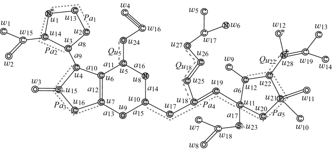
Figure 2: An illustration of a hydrogen-suppressed chemical graph $\langle\mathbb{C}\rangle$ obtained from a chemical graph $\mathbb{C}$ with $\mathrm{r}(\mathbb{C})=4$ by removing all the hydrogens, where for ${\rho}=2$, $V^{\mathrm{ex}}(\mathbb{C})=\{w_{i}\mid i\in[1,19]\}$ and $V^{\mathrm{int}}(\mathbb{C})=\{u_{i}\mid i\in[1,28]\}$.

3 Two-layered Model

This section reviews the two-layered model and describes our modification to the model.

Let $\mathbb{C}=(H,\alpha,\beta)$ be a chemical graph and ${\rho}\geq 1$ be an integer, which we call a branch-parameter.

A two-layered model of $\mathbb{C}$ is a partition of the hydrogen-suppressed chemical graph $\langle\mathbb{C}\rangle$ into an “interior” and an “exterior” in the following way. We call a vertex $v\in V(\langle\mathbb{C}\rangle)$ (resp., an edge $e\in E(\langle\mathbb{C}\rangle))$ of $G$ an exterior-vertex (resp., exterior-edge) if $\mathrm{ht}(v)<{\rho}$ (resp., $e$ is incident to an exterior-vertex) and denote the sets of exterior-vertices and exterior-edges by $V^{\mathrm{ex}}(\mathbb{C})$ and $E^{\mathrm{ex}}(\mathbb{C})$, respectively and denote $V^{\mathrm{int}}(\mathbb{C})=V(\langle\mathbb{C}\rangle)\setminus V^{\mathrm{ex}}(\mathbb{C})$ and $E^{\mathrm{int}}(\mathbb{C})=E(\langle\mathbb{C}\rangle)\setminus E^{\mathrm{ex}}(\mathbb{C})$, respectively. We call a vertex in $V^{\mathrm{int}}(\mathbb{C})$ (resp., an edge in $E^{\mathrm{int}}(\mathbb{C})$) an interior-vertex (resp., interior-edge). The set $E^{\mathrm{ex}}(\mathbb{C})$ of exterior-edges forms a collection of connected graphs each of which is regarded as a rooted tree $T$ rooted at the vertex $v\in V(T)$ with the maximum $\mathrm{ht}(v)$. Let $\mathcal{T}^{\mathrm{ex}}(\langle\mathbb{C}\rangle)$ denote the set of these chemical rooted trees in $\langle\mathbb{C}\rangle$. The interior $\mathbb{C}^{\mathrm{int}}$ of $\mathbb{C}$ is defined to be the subgraph $(V^{\mathrm{int}}(\mathbb{C}),E^{\mathrm{int}}(\mathbb{C}))$ of $\langle\mathbb{C}\rangle$.

Figure 2 illustrates an example of a hydrogen-suppressed chemical graph $\langle\mathbb{C}\rangle$. For a branch-parameter ${\rho}=2$, the interior of the chemical graph $\langle\mathbb{C}\rangle$ in Figure 2 is obtained by removing the set of vertices with degree 1 ${\rho}=2$ times; i.e., first remove the set $V_{1}=\{w_{1},w_{2},\ldots,w_{14}\}$ of vertices of degree 1 in $\langle\mathbb{C}\rangle$ and then remove the set $V_{2}=\{w_{15},w_{16},\ldots,w_{19}\}$ of vertices of degree 1 in $\langle\mathbb{C}\rangle-V_{1}$, where the removed vertices become the exterior-vertices of $\langle\mathbb{C}\rangle$.

For each interior-vertex $u\in V^{\mathrm{int}}(\mathbb{C})$, let $T_{u}\in\mathcal{T}^{\mathrm{ex}}(\langle\mathbb{C}\rangle)$ denote the chemical tree rooted at $u$ (where possibly $T_{u}$ consists of vertex $u$) and define the $\rho$-fringe-tree $\mathbb{C}[u]$ to be the chemical rooted tree obtained from $T_{u}$ by putting back the hydrogens originally attached $T_{u}$ in $\mathbb{C}$. Let $\mathcal{T}(\mathbb{C})$ denote the set of $\rho$-fringe-trees $\mathbb{C}[u],u\in V^{\mathrm{int}}(\mathbb{C})$. Figure 3 illustrates the set $\mathcal{T}(\mathbb{C})=\{\mathbb{C}[u_{i}]\mid i\in[1,28]\}$ of the 2-fringe-trees of the example $\mathbb{C}$ in Figure 2.

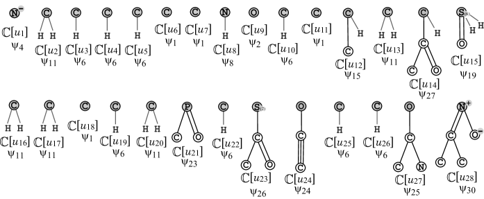
Figure 3: The set $\mathcal{T}(\mathbb{C})$ of 2-fringe-trees $\mathbb{C}[u_{i}],i\in[1,28]$ of the example $\mathbb{C}$ in Figure 2, where the root of each tree is depicted with a gray circle and the hydrogens attached to non-root vertices are omitted in the figure.

Feature Function  The feature of an interior-edge $e=uv\in E^{\mathrm{int}}(\mathbb{C})$ such that $\alpha(u)={\tt a}$, $\deg_{\langle\mathbb{C}\rangle}(u)=d$, $\alpha(v)={\tt b}$, $\deg_{\langle\mathbb{C}\rangle}(v)=d^{\prime}$ and $\beta(e)=m$ is represented by a tuple $({\tt a}d,{\tt b}d^{\prime},m)$, which is called the edge-configuration of the edge $e$, where we call the tuple $({\tt a},{\tt b},m)$ the adjacency-configuration of the edge $e$.

For an integer $K$, a feature vector $f(\mathbb{C})$ of a chemical graph $\mathbb{C}$ is defined by a feature function $f$ that consists of $K$ descriptors. We call $\mathbb{R}^{K}$ the feature space.

Tanaka et al. [26] defined a feature vector $f(\mathbb{C})\in\mathbb{R}^{K}$ to be a combination of the frequency of edge-configurations of the interior-edges and the frequency of chemical rooted trees among the set of chemical rooted trees $\mathbb{C}[u]$ over all interior-vertices $u$. In this paper, we introduce the rank and the adjacency-configuration of leaf-edges as new descriptors in a feature vector of a chemical graph.

Topological Specification  A topological specification is described as a set of the following rules proposed by [25] and modified by Tanaka et al. [26]:

1. a seed graph $G_{\mathrm{C}}$ as an abstract form of a target chemical graph $\mathbb{C}$;

2. a set $\mathcal{F}$ of chemical rooted trees as candidates for a tree $\mathbb{C}[u]$ rooted at each interior-vertex $u$ in $\mathbb{C}$; and

3. lower and upper bounds on the number of components in a target chemical graph such as chemical elements, double/triple bonds and the interior-vertices in $\mathbb{C}$.

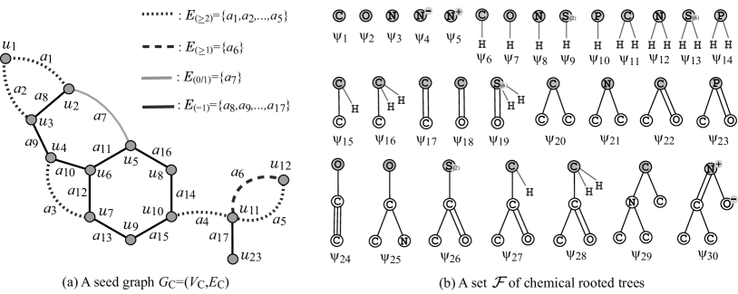
Figure 4: (a) An illustration of a seed graph $G_{\mathrm{C}}$ with $\mathrm{r}(G_{\mathrm{C}})=5$ where the vertices in $V_{\mathrm{C}}$ are depicted with gray circles, the edges in $E_{(\geq 2)}$ are depicted with dotted lines, the edges in $E_{(\geq 1)}$ are depicted with dashed lines, the edges in $E_{(0/1)}$ are depicted with gray bold lines and the edges in $E_{(=1)}$ are depicted with black solid lines; (b) A set $\mathcal{F}=\{\psi_{1},\psi_{2},\ldots,\psi_{30}\}\subseteq\mathcal{F}(D_{\pi})$ of 30 chemical rooted trees $\psi_{i},i\in[1,30]$, where the root of each tree is depicted with a gray circle, where the hydrogens attached to non-root vertices are omitted in the figure.

Figure 4(a) and (b) illustrate examples of a seed graph $G_{\mathrm{C}}$ and a set $\mathcal{F}$ of chemical rooted trees, respectively. Given a seed graph $G_{\mathrm{C}}$, the interior of a target chemical graph $\mathbb{C}$ is constructed from $G_{\mathrm{C}}$ by replacing some edges $a=uv$ with paths $P_{a}$ between the end-vertices $u$ and $v$ and by attaching new paths $Q_{v}$ to some vertices $v$. For example, a chemical graph $C$ in Figure 2 is constructed from the seed graph $G_{\mathrm{C}}$ in Figure 4(a) as follows.

1. First replace five edges $a_{1}=u_{1}u_{2},a_{2}=u_{1}u_{3},a_{3}=u_{4}u_{7},a_{4}=u_{10}u_{11}$ and $a_{5}=u_{11}u_{12}$ in $G_{\mathrm{C}}$ with new paths $P_{a_{1}}=(u_{1},u_{13},u_{2})$, $P_{a_{2}}=(u_{1},u_{14},u_{3})$, $P_{a_{3}}=(u_{4},u_{15},u_{16},u_{7})$, $P_{a_{4}}=(u_{10},u_{17},u_{18},u_{19},u_{11})$ and $P_{a_{5}}=(u_{11},u_{20},u_{21},u_{22},u_{12})$, respectively to obtain a subgraph $G_{1}$ of $\langle\mathbb{C}\rangle$.

2. Next attach to this graph $G_{1}$ three new paths $Q_{u_{5}}=(u_{5},u_{24})$, $Q_{u_{18}}=(u_{18},u_{25},u_{26},u_{27})$ and $Q_{u_{22}}=(u_{22},u_{28})$ to obtain the interior of $\langle\mathbb{C}\rangle$ in Figure 2.

3. Finally attach to the interior 28 trees selected from the set $\mathcal{F}$ and assign chemical elements and bond-multiplicities in the interior to obtain a chemical graph $\mathbb{C}$ in Figure 2. In Figure 3, XXX Check the next again XXXX $\psi_{1}\in\mathcal{F}$ is selected for $\mathbb{C}[u_{i}]$, $i\in\{6,7,11\}$. Similarly $\psi_{2}$ for $\mathbb{C}[u_{9}]$, $\psi_{4}$ for $\mathbb{C}[u_{i}]$, $i\in\{3,4,5,10,18,19,22,25,26\}$, $\psi_{5}$ for $\mathbb{C}[u_{i}]$, $i\in\{2,13,16,17,20\}$, $\psi_{7}$ for $\mathbb{C}[u_{i}]$, $i\in\{1,8\}$, $\psi_{9}$ for $\mathbb{C}[u_{12}]$, $\psi_{11}$ for $\mathbb{C}[u_{15}]$, $\psi_{13}$ for $\mathbb{C}[u_{21}]$, $\psi_{16}$ for $\mathbb{C}[u_{24}]$, $\psi_{17}$ for $\mathbb{C}[u_{27}]$, $\psi_{18}$ for $\mathbb{C}[u_{14}]$, $\psi_{19}$ for $\mathbb{C}[u_{23}]$ and $\psi_{21}$ for $\mathbb{C}[u_{28}]$.

Our definition of a topological specification is analogous with the one by Tanaka et al. [26] except for a necessary modification due to the introduction of multiple valences of chemical elements, cations and anions (see Appendix B for a full description of topological specification).

4 Linear Regressions

For an integer $p\geq 1$ and a vector $x\in\mathbb{R}^{p}$, the $j$-th entry of $x$ is denoted by $x(j),j\in[1,p]$.

Let $D$ be a data set of chemical graphs $\mathbb{C}$ with an observed value $a(\mathbb{C})\in\mathbb{R}$, where we denote by $a_{i}=a(\mathbb{C}_{i})$ for an indexed graph $\mathbb{C}_{i}$.

Let $f$ be a feature function that maps a chemical graph $\mathbb{C}$ to a vector $f(\mathbb{C})\in\mathbb{R}^{K}$ where we denote by $x_{i}=f(\mathbb{C}_{i})$ for an indexed graph $\mathbb{C}_{i}$. For a prediction function $\eta:\mathbb{R}^{K}\to\mathbb{R}$, define an error function

$$\mathrm{Err}(\eta;D)\triangleq\sum_{\mathbb{C}_{i}\in D}(a_{i}-\eta(f(\mathbb{C}_{i})))^{2}=\sum_{\mathbb{C}_{i}\in D}(a_{i}-\eta(x_{i}))^{2},$$

and define the coefficient of determination $\mathrm{R}^{2}(\eta,D)$ to be

$${\mathrm{R}^{2}(\eta,D)\triangleq 1-\frac{\mathrm{Err}(\eta;D)}{\sum_{\mathbb{C}_{i}\in D}(a_{i}-\widetilde{a})^{2}}\mbox{ for }\widetilde{a}=\frac{1}{|D|}\sum_{\mathbb{C}\in D}a(\mathbb{C}).}$$

For a feature space $\mathbb{R}^{K}$, a hyperplane is defined to be a pair $(w,b)$ of a vector $w\in\mathbb{R}^{K}$ and a real $b\in\mathbb{R}$. Given a hyperplane $(w,b)\in\mathbb{R}^{K+1}$, a prediction function $\eta_{w,b}:\mathbb{R}^{K}\to\mathbb{R}$ is defined by setting

$$\eta_{w,b}(x)\triangleq w\cdot x+b=\sum_{j\in[1,K]}w(j)x(j)+b.$$

We can observe that such a prediction function can be represented as an ANN with an input layer with $K$ nodes $u_{j},j\in[1,K]$ and an output layer with a single node $v$ such that the weight of edge arc $(u_{j},v)$ is set to be $w(j)$, the bias of node $u$ is set to be $b$ and the activation function at node $u$ is set to be a linear function. However, a learning algorithm for an ANN may not find a set of weights $w(j),j\in[1,K]$ and $b$ that minimizes the error function, since the algorithm simply iterates modification of the current weights and biases until it terminates at a local optima in the minimization.

We wish to find a hyperplane $(w,b)$ that minimizes the error function $\mathrm{Err}(\eta_{w,b};D)$. In many cases, a feature vector $f$ contains descriptors that do not play an essential role in constructing a good prediction function. When we solve the minimization problem, the entries $w(j)$ for some descriptors $j\in[1,K]$ in the resulting hyperplane $(w,b)$ become zero, which means that these descriptors were not necessarily important for finding a prediction function $\eta_{w,b}$. It is proposed that solving the minimization with an additional penalty term $\tau$ to the error function often results in a more number of entries $w(j)=0$, reducing a set of descriptors necessary for defining a prediction function $\eta_{w,b}$. For an error function with such a penalty term, a Ridge function $\frac{1}{2|D|}\mathrm{Err}(\eta_{w,b};D)+\lambda[\sum_{j\in[1,K]}w(j)^{2}+b^{2}]$ [27] and a Lasso function $\frac{1}{2|D|}\mathrm{Err}(\eta_{w,b};D)+\lambda[\sum_{j\in[1,K]}|w(j)|+|b|]$ [28] are known, where $\lambda\in\mathbb{R}$ is a given real number.

Given a prediction function $\eta_{w,b}$, we can simulate a process of computing the output $\eta_{w,b}(x)$ for an input $x\in\mathbb{R}^{K}$ as an MILP $\mathcal{M}(x,y;\mathcal{C}_{1})$ in the framework. By solving such an MILP for a specified target value $y^{*}$ , we can find a vector $x^{*}\in\mathbb{R}^{K}$ such that $\eta_{w,b}(x^{*})=y^{*}$. Instead of specifying a single target value $y^{*}$, we use lower and upper bounds $\underline{y}^{*},\overline{y}^{*}\in\mathbb{R}$ on the value $a(\mathbb{C})$ of a chemical graph $\mathbb{C}$ to be inferred. We can control the range between $\underline{y}^{*}$ and $\overline{y}^{*}$ for searching a chemical graph $\mathbb{C}$ by setting $\underline{y}^{*}$ and $\overline{y}^{*}$ to be close or different values. A desired MILP is formulated as follows.

$\mathcal{M}(x,y;\mathcal{C}_{1})$: An MILP formulation for the inverse problem to prediction function

constants:

1. A hyperplane $(w,b)$ with $w\in\mathbb{R}^{K}$ and $b\in\mathbb{R}$;

2. Real values $\underline{y}^{*},\overline{y}^{*}\in\mathbb{R}$ such that $\underline{y}^{*}<\overline{y}^{*}$;

3. A set $I_{\mathbb{Z}}$ of indices $j\in[1,K]$ such that the $j$-th descriptor $\mathrm{dcp}_{j}(\mathbb{C})$ is always an integer;

4. A set $I_{+}$ of indices $j\in[1,K]$ such that the $j$-th descriptor $\mathrm{dcp}_{j}(\mathbb{C})$ is always non-negative;

5. $\ell(j),u(j)\in\mathbb{R},j\in[1,K]$: lower and upper bounds on the $j$-th descriptor;

variables:

1. Non-negative integer variable $x(j)\in\mathbb{Z}_{+},j\in I_{\mathbb{Z}}\cap I_{+}$;

2. Integer variable $x(j)\in\mathbb{Z},j\in I_{\mathbb{Z}}\setminus I_{+}$;

3. Non-negative real variable $x(j)\in\mathbb{Z}_{+},j\in I_{+}\setminus I_{\mathbb{Z}}$;

4. Real variable $x(j)\in\mathbb{Z},j\in[1,K]\setminus(I_{\mathbb{Z}}\cup I_{+})$;

constraints:

$$\ell(j)\leq x(j)\leq u(j),j\in[1,K],$$ (1)

$$\underline{y}^{*}\leq\sum_{j\in[1,K]}w(j)x(j)+b\leq\overline{y}^{*},$$ (2)

objective function:
   none.

The number of variables and constraints in the above MILP formulation is $O(K)$. It is not difficult to see that the above MILP is an NP-hard problem.

The entire MILP for Stage 4 consists of the two MILPs $\mathcal{M}(x,y;\mathcal{C}_{1})$ and $\mathcal{M}(g,x;\mathcal{C}_{2})$ with no objective function. The latter represents the computation process of our feature function $f$ and a given topological specification. See Appendix D for the details of MILP $\mathcal{M}(g,x;\mathcal{C}_{2})$.

5 Results

We implemented our method of Stages 1 to 5 for inferring chemical graphs under a given topological specification and conducted experiments to evaluate the computational efficiency. We executed the experiments on a PC with Processor: Core i7-9700 (3.0 GHz; 4.7 GHz at the maximum) and Memory: 16 GB RAM DDR4.

Results on Phase 1. We have conducted experiments of linear regression for 37 chemical properties among which we report the following 18 properties to which the test coefficient of determination ${\rm R}^{2}$ attains at least 0.8: octanol/water partition coefficient (Kow), heat of combustion (Hc), vapor density (Vd), optical rotation (OptR), electron density on the most positive atom (EDPA), melting point (Mp), heat of atomization (Ha), heat of formation (Hf), internal energy at 0K (U0), energy of lowest unoccupied molecular orbital (Lumo), isotropic polarizability (Alpha), heat capacity at 298.15K (Cv), solubility (Sl), surface tension (SfT), viscosity (Vis), isobaric heat capacities in liquid phase (IhcLiq), isobaric heat capacities in solid phase (IhcSol) and lipophilicity (Lp).

We used data sets provided by HSDB from PubChem [29] for Kow, Hc, Vd and OptR, M. Jalali-Heravi and M. Fatemi [30] for EDPA, Roy and Saha [31] for Mp, Ha and Hf, MoleculeNet [32] for U0, Lumo, Alpha, Cv and Sl, Goussard et al. [33] for SfT and Vis, R. Naef [34] for IhcLiq and IhcSol, and Figshare [35] for Lp.

Properties U0, Lumo, Alpha and Cv share a common original data set $D^{*}$ with more than 130,000 compounds, and we used a set $D_{\pi}$ of 1,000 graphs randomly selected from $D^{*}$ as a common data set of these four properties $\pi$ in this experiment.

We implemented Stages 1, 2 and 3 in Phase 1 as follows.

Stage 1. We set a graph class $\mathcal{G}$ to be the set of all chemical graphs with any graph structure, and set a branch-parameter ${\rho}$ to be 2.

For each of the properties, we first select a set $\Lambda$ of chemical elements and then collect a data set $D_{\pi}$ on chemical graphs over the set $\Lambda$ of chemical elements. To construct the data set $D_{\pi}$, we eliminated chemical compounds that do not satisfy one of the following: the graph is connected, the number of carbon atoms is at least four, and the number of non-hydrogen neighbors of each atom is at most 4.

Table 1 shows the size and range of data sets that we prepared for each chemical property in Stage 1, where we denote the following:

1. $\Lambda$: the set of elements used in the data set $D_{\pi}$; $\Lambda$ is one of the following 11 sets: $\Lambda_{1}=\{{\tt H},{\tt C},{\tt O}\}$; $\Lambda_{2}=\{{\tt H},{\tt C},{\tt O},{\tt N}\}$; $\Lambda_{3}=\{{\tt H},{\tt C},{\tt O},{\tt S}_{(2)}\}$; $\Lambda_{4}=\{{\tt H},{\tt C},{\tt O},{\tt Si}\}$;
   $\Lambda_{5}=\{{\tt H},{\tt C},{\tt O},{\tt N},{\tt Cl},{\tt P}_{(3)},{\tt P}_{(5)}\}$; $\Lambda_{6}=\{{\tt H},{\tt C},{\tt O},{\tt N},{\tt S}_{(2)},{\tt F}\}$; $\Lambda_{7}=\{{\tt H},{\tt C},{\tt O},{\tt N},{\tt S}_{(2)},{\tt S}_{(6)},{\tt Cl}\}$; $\Lambda_{8}=\{{\tt H},{\tt C}_{(2)},{\tt C}_{(3)},{\tt C}_{(4)},{\tt O},{\tt N}_{(2)},{\tt N}_{(3)}\}$; $\Lambda_{9}=\{{\tt H},{\tt C},{\tt O},{\tt N},{\tt S}_{(2)},{\tt S}_{(4)},{\tt S}_{(6)},{\tt Cl}\}$;
   $\Lambda_{10}=\{{\tt H},{\tt C}_{(2)},{\tt C}_{(3)},{\tt C}_{(4)},{\tt C}_{(5)},{\tt O},{\tt N}_{(1)},{\tt N}_{(2)},{\tt N}_{(3)},{\tt F}\}$; and
   $\Lambda_{11}=\{{\tt H},{\tt C}_{(2)},{\tt C}_{(3)},{\tt C}_{(4)},{\tt O},{\tt N}_{(2)},{\tt N}_{(3)},{\tt S}_{(2)},{\tt S}_{(4)},{\tt S}_{(6)},{\tt Cl}\}$, where ${\tt e}_{(i)}$ for a chemical element ${\tt e}$ and an integer $i\geq 1$ means that a chemical element ${\tt e}$ with valence $i$.

2. $|D_{\pi}|$: the size of data set $D_{\pi}$ over $\Lambda$ for the property $\pi$.

3. $\underline{n},~{}\overline{n}$: the minimum and maximum values of the number $n(\mathbb{C})$ of non-hydrogen atoms in compounds $\mathbb{C}$ in $D_{\pi}$.

4. $\underline{a},~{}\overline{a}$: the minimum and maximum values of $a(\mathbb{C})$ for $\pi$ over compounds $\mathbb{C}$ in $D_{\pi}$.

5. $|\Gamma|$: the number of different edge-configurations of interior-edges over the compounds in $D_{\pi}$.

6. $|\mathcal{F}|$: the number of non-isomorphic chemical rooted trees in the set of all 2-fringe-trees in the compounds in $D_{\pi}$.

7. $K$: the number of descriptors in a feature vector $f(\mathbb{C})$.

Stage 2. We used the new feature function defined in our chemical model without suppressing hydrogen (see Appendix A for the detail). We standardize the range of each descriptor and the range $\{t\in\mathbb{R}\mid\underline{a}\leq t\leq\overline{a}\}$ of property values $a(\mathbb{C}),\mathbb{C}\in D_{\pi}$.

Stage 3. For each chemical property $\pi$, we select a penalty value $\lambda_{\pi}$ in the Lasso function from 36 different values from 0 to 100 by conducting linear regression as a preliminary experiment.

We conducted an experiment in Stage 3 to evaluate the performance of the prediction function based on cross-validation. For a property $\pi$, an execution of a cross-validation consists of five trials of constructing a prediction function as follows. First partition the data set $D_{\pi}$ into five subsets $D^{(k)}$, $k\in[1,5]$ randomly. For each $k\in[1,5]$, the $k$-th trial constructs a prediction function $\eta^{(k)}$ by conducting a linear regression with the penalty term $\lambda_{\pi}$ using the set $D_{\pi}\setminus D^{(k)}$ as a training data set. We used scikit-learn version 0.23.2 with Python 3.8.5 for executing linear regression with Lasso function. For each property, we executed ten cross-validations and we show the median of test $\mathrm{R}^{2}(\eta^{(k)},D^{(k)}),k\in[1,5]$ over all ten cross-validations. Recall that a subset of descriptors is selected in linear regression with Lasso function and let $K^{\prime}$ denote the average number of selected descriptors over all 50 trials. The running time per trial in a cross-validation was at most one second.

Table 1: Results in Phase 1.

$\pi$	$\Lambda$	$|D_{\pi}|$	$\underline{n},~{}\overline{n}$	$\underline{a},~{}\overline{a}$	$|\Gamma|$	$|\mathcal{F}|$	$K$	$\lambda_{\pi}$	$K^{\prime}$	test $\mathrm{R}^{2}$
Kow	$\Lambda_{2}$	684	4, 58	-7.5, 15.6	25	166	223	$6.4\mathrm{E}{-5}$	80.3	0.953
Kow	$\Lambda_{9}$	899	4, 69	-7.5, 15.6	37	219	303	$5.5\mathrm{E}{-5}$	112.1	0.927
Hc	$\Lambda_{2}$	255	4, 63	49.6, 35099.6	17	106	154	$1.9\mathrm{E}{-4}$	19.2	0.946
Hc	$\Lambda_{7}$	282	4, 63	49.6, 35099.6	21	118	177	$1.9\mathrm{E}{-4}$	20.5	0.951
Vd	$\Lambda_{2}$	474	4, 30	0.7, 20.6	21	160	214	$1.0\mathrm{E}{-3}$	3.6	0.927
Vd	$\Lambda_{5}$	551	4, 30	0.7, 20.6	24	191	256	$5.5\mathrm{E}{-4}$	8.0	0.942
OptR	$\Lambda_{2}$	147	5, 44	-117.0, 165.0	21	55	107	$4.6\mathrm{E}{-4}$	39.2	0.823
OptR	$\Lambda_{6}$	157	5, 69	-117.0, 165.0	25	62	123	$7.3\mathrm{E}{-4}$	41.7	0.825
EDPA	$\Lambda_{1}$	52	11, 16	0.80, 3.76	9	33	64	$1.0\mathrm{E}{-4}$	10.9	0.999
Mp	$\Lambda_{2}$	467	4, 122	-185.33, 300.0	23	142	197	$3.7\mathrm{E}{-5}$	82.5	0.817
Ha	$\Lambda_{3}$	115	4, 11	1100.6, 3009.6	8	83	115	$3.7\mathrm{E}{-5}$	39.0	0.997
Hf	$\Lambda_{1}$	82	4, 16	30.2, 94.8	5	50	74	$1.0\mathrm{E}{-4}$	34.0	0.987
U0	$\Lambda_{10}$	977	4, 9	-570.6, -272.8	59	190	297	$1.0\mathrm{E}{-7}$	246.7	0.999
Lumo	$\Lambda_{10}$	977	4, 9	-0.11, 0.10	59	190	297	$6.4\mathrm{E}{-5}$	133.9	0.841
Alpha	$\Lambda_{10}$	977	4, 9	50.9, 99.6	59	190	297	$1.0\mathrm{E}{-5}$	125.5	0.961
Cv	$\Lambda_{10}$	977	4, 9	19.2, 44.0	59	190	297	$1.0\mathrm{E}{-5}$	165.3	0.961
Sl	$\Lambda_{9}$	915	4, 55	-11.6, 1.11	42	207	300	$7.3\mathrm{E}{-5}$	130.6	0.808
SfT	$\Lambda_{4}$	247	5, 33	12.3, 45.1	11	91	128	$6.4\mathrm{E}{-4}$	20.9	0.804
Vis	$\Lambda_{4}$	282	5, 36	-0.64, 1.63	12	88	126	$8.2\mathrm{E}{-4}$	16.3	0.893
IhcLiq	$\Lambda_{2}$	770	4, 78	106.3, 1956.1	23	200	256	$1.9\mathrm{E}{-5}$	82.2	0.987
IhcLiq	$\Lambda_{7}$	865	4, 78	106.3, 1956.1	29	246	316	$8.2\mathrm{E}{-6}$	139.1	0.986
IhcSol	$\Lambda_{8}$	581	5, 70	67.4, 1220.9	33	124	192	$2.8\mathrm{E}{-5}$	75.9	0.985
IhcSol	$\Lambda_{11}$	668	5, 70	67.4, 1220.9	40	140	228	$2.8\mathrm{E}{-5}$	86.7	0.982
Lp	$\Lambda_{2}$	615	6, 60	-3.62, 6.84	32	116	186	$1.0\mathrm{E}{-4}$	98.5	0.856
Lp	$\Lambda_{9}$	936	6, 74	-3.62, 6.84	44	136	231	$6.4\mathrm{E}{-5}$	130.4	0.840

Table 1 shows the results on Stages 2 and 3, where we denote the following:

1. $\lambda_{\pi}$: the penalty value in the Lasso function selected for a property $\pi$, where $a\mathrm{E}{b}$ means $a\times 10^{b}$.

2. $K^{\prime}$: the average of the number of descriptors selected in the linear regression over all 50 trials in ten cross-validations.

3. test $\mathrm{R}^{2}$: the median of test $\mathrm{R}^{2}$ over all 50 trials in ten cross-validations.

Recall that the adjacency-configuration for leaf-edges was introduced as a new descriptor in this paper. Without including this new descriptor, the test $\mathrm{R}^{2}$ for property Vis was 0.790, that for Lumo was 0.799 and that for Mp was 0.796, while the test $\mathrm{R}^{2}$ for each of the other properties in Table 1 was almost the same.

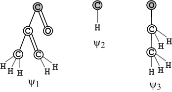
Figure 5: An illustration of chemical rooted trees $\psi_{1}$, $\psi_{1}$ and $\psi_{3}$ that are selected in Lasso linear regression for constructing a prediction function to property Vd, where the root is depicted with a gray circle.

From Table 1, we observe that a relatively large number of properties admit a good prediction function based on linear regression. The number $K^{\prime}$ of descriptors used in linear regression is considerably small for some properties. For example of property Vd,

1. the four descriptors most frequently selected in the case of $\Lambda=\{{\tt H},{\tt O},{\tt C},{\tt N}\}$ are the number of non-hydrogen atoms; the number of interior-vertices $v$ with $\deg_{\mathbb{C}^{\mathrm{int}}}(v)=1$; the number of fringe-trees r-isomorphic to the chemical rooted tree $\psi_{1}$ in Figure 5; and the number of leaf-edges with adjacency-configuration $({\tt O},{\tt C},2)$.

2. the eight descriptors most frequently selected in the case of $\Lambda=\{{\tt H},{\tt O},{\tt C},{\tt N},{\tt Cl},{\tt P}_{(3)},{\tt P}_{(5)}\}$ are the number of non-hydrogen atoms; the number of interior-vertices $v$ with $\deg_{\mathbb{C}^{\mathrm{int}}}(v)=1$; the number of exterior-vertices $v$ with $\alpha(v)={\tt Cl}$; the number of interior-edges with edge-configuration $\gamma_{i},i=1,2$, where $\gamma_{1}=({\tt C}2,{\tt C}2,2)$ and $\gamma_{2}=({\tt C}3,{\tt C}4,1)$; and the number of fringe-trees r-isomorphic to the chemical rooted tree $\psi_{i},i=1,2,3$ in Figure 5.

Results on Phase 2. To execute Stages 4 and 5 in Phase 2, we used a set of seven instances $I_{\mathrm{a}}$, $I_{\mathrm{b}}^{i},i\in[1,4]$, $I_{\mathrm{c}}$ and $I_{\mathrm{d}}$ based on seed graphs prepared by Shi et al. [25]. We here present their seed graphs $G_{\mathrm{C}}$ (see Appendix B for the details of $I_{\mathrm{a}}$ and Appendix C for the details of $I_{\mathrm{b}}^{i},i\in[1,4]$, $I_{\mathrm{c}}$ and $I_{\mathrm{d}}$). The seed graph $G_{\mathrm{C}}$ of instance $I_{\mathrm{a}}$ is given by the graph in Figure 4(a). The seed graph $G_{\mathrm{C}}^{1}$ (resp., $G_{\mathrm{C}}^{i},i=2,3,4$) of instances $I_{\mathrm{b}}^{1}$ and $I_{\mathrm{d}}$ (resp., $I_{\mathrm{b}}^{i},i=2,3,4$) is illustrated in Figure 6.

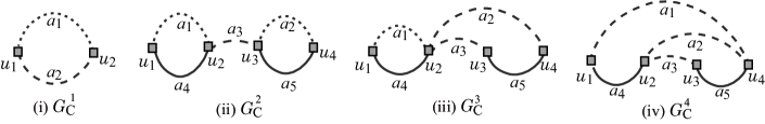
Figure 6: (i) Seed graph $G_{\mathrm{C}}^{1}$ for $I_{\mathrm{b}}^{1}$ and $I_{\mathrm{d}}$; (ii) Seed graph $G_{\mathrm{C}}^{2}$ for $I_{\mathrm{b}}^{2}$; (iii) Seed graph $G_{\mathrm{C}}^{3}$ for $I_{\mathrm{b}}^{3}$; (iv) Seed graph $G_{\mathrm{C}}^{4}$ for $I_{\mathrm{b}}^{4}$.

Instance $I_{\mathrm{c}}$ has been introduced in order to infer a chemical graph $\mathbb{C}^{\dagger}$ such that the core of $\mathbb{C}^{\dagger}$ is equal to the core of chemical graph $\mathbb{C}_{A}$: CID 24822711 in Figure 7(a) and the frequency of each edge-configuration in the non-core of $\mathbb{C}^{\dagger}$ is equal to that of chemical graph $\mathbb{C}_{B}$: CID 59170444 in Figure 7(b). This means that the seed graph $G_{\mathrm{C}}$ of $I_{\mathrm{c}}$ is the core of $\mathbb{C}_{A}$ which is indicated by a shaded area in Figure 7(a).

Instance $I_{\mathrm{d}}$ has been introduced in order to infer a chemical monocyclic graph $\mathbb{C}^{\dagger}$ such that the frequency vector of edge-configurations in $\mathbb{C}^{\dagger}$ is a vector obtained by merging those of chemical graphs $\mathbb{C}_{A}$: CID 10076784 and $\mathbb{C}_{B}$: CID 44340250 in Figure 7(c) and (d), respectively.

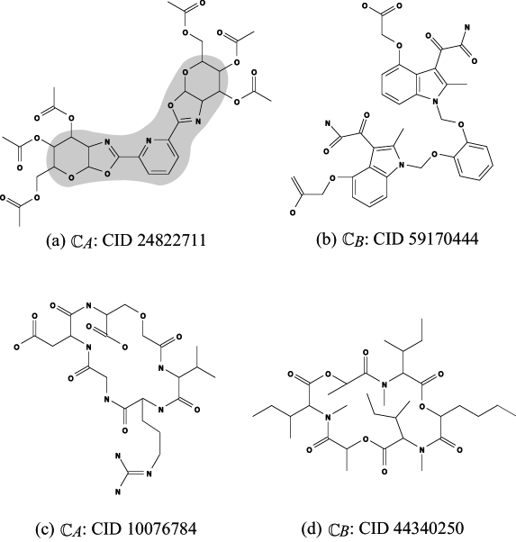
Figure 7: An illustration of chemical compounds for instances $I_{\rm c}$ and $I_{\rm d}$: (a) $\mathbb{C}_{A}$: CID 24822711; (b) $\mathbb{C}_{B}$: CID 59170444; (c) $\mathbb{C}_{A}$: CID 10076784; (d) $\mathbb{C}_{B}$: CID 44340250, where hydrogens are omitted.

Stage 4. We executed Stage 4 for five properties $\pi\in\{$Hc, Vd, OptR, IhcLiq, Vis$\}$.

For the MILP formulation $\mathcal{M}(x,y;\mathcal{C}_{1})$ in Section 4, we use the prediction function $\eta_{w,b}$ that attained the median test $\mathrm{R}^{2}$ in Table 1. To solve an MILP in Stage 4, we used CPLEX version 12.10. Tables 2 to 6 show the computational results of the experiment in Stage 4 for the five properties, where we denote the following:

1. $\underline{y}^{*},~{}\overline{y}^{*}$: lower and upper bounds $\underline{y}^{*},\overline{y}^{*}\in\mathbb{R}$ on the value $a(\mathbb{C})$ of a chemical graph $\mathbb{C}$ to be inferred;

2. $\#$v (resp., $\#$c): the number of variables (resp., constraints) in the MILP in Stage 4;

3. I-time: the time (sec.) to solve the MILP in Stage 4;

4. $n$: the number $n(\mathbb{C}^{\dagger})$ of non-hydrogen atoms in the chemical graph $\mathbb{C}^{\dagger}$ inferred in Stage 4; and

5. $\mathrm{n}^{\mathrm{int}}$: the number $\mathrm{n}^{\mathrm{int}}(\mathbb{C}^{\dagger})$ of interior-vertices in the chemical graph $\mathbb{C}^{\dagger}$ inferred in Stage 4;

6. $\eta(f(\mathbb{C}^{\dagger}))$: the predicted property value $\eta(f(\mathbb{C}^{\dagger}))$ of the chemical graph $\mathbb{C}^{\dagger}$ inferred in Stage 4.

Table 2: Results of Stages 4 and 5 for Hc.

inst.	$\underline{y}^{*},~{}\overline{y}^{*}$	$\#$v	$\#$c	I-time	$n$	​​$\mathrm{n}^{\mathrm{int}}$	$\eta(f(\mathbb{C}^{\dagger}))$​​	D-time	$\mathbb{C}$-LB	$\#\mathbb{C}$
$I_{\mathrm{a}}$	5950, 6050	9902	9255	4.6	44	25	5977.9	0.068	1	1
$I_{\mathrm{b}}^{1}$	5950, 6050	9404	6776	1.7	36	10	6007.1	0.048	6	6
$I_{\mathrm{b}}^{2}$	5950, 6050	11729	9891	16.7	50	25	6043.7	38.7	$2.4\!\!\times\!\!10^{5}$	100
$I_{\mathrm{b}}^{3}$	5950, 6050	11510	9894	16.3	47	25	6015.4	0.353	8724	100
$I_{\mathrm{b}}^{4}$	5950, 6050	11291	9897	9.0	49	26	5971.6	0.304	84	84
$I_{\mathrm{c}}$	13700, 13800	6915	7278	0.7	50	33	13703.3	0.016	1	1
$I_{\mathrm{d}}$	13700, 13800	5535	6781	4.9	44	23	13704.7	0.564	$4.3\!\!\times\!\!10^{5}$	100

Figure 8(a) illustrates the chemical graph $\mathbb{C}^{\dagger}$ inferred from $I_{\mathrm{c}}$ with $(\underline{y}^{*},\overline{y}^{*})=(13700,13800)$ of Hc in Table 2.

Table 3: Results of Stages 4 and 5 for Vd.

inst.	$\underline{y}^{*},~{}\overline{y}^{*}$	$\#$v	$\#$c	I-time	$n$	​​$\mathrm{n}^{\mathrm{int}}$	$\eta(f(\mathbb{C}^{\dagger}))$​​	D-time	$\mathbb{C}$-LB	$\#\mathbb{C}$
$I_{\mathrm{a}}$	16, 17	9481	9358	1.6	38	23	16.83	0.070	1	1
$I_{\mathrm{b}}^{1}$	16, 17	9928	6986	1.5	35	12	16.68	0.206	48	48
$I_{\mathrm{b}}^{2}$	21, 22	12373	10101	10.0	48	25	21.62	0.104	20	20
$I_{\mathrm{b}}^{3}$	21, 22	12159	10104	6.5	48	25	21.95	3.65	$8.6\!\!\times\!\!10^{5}$	100
$I_{\mathrm{b}}^{4}$	21, 22	11945	10107	8.1	48	25	21.34	0.057	6	6
$I_{\mathrm{c}}$	21, 22	7073	7438	0.7	50	34	21.89	0.016	1	1
$I_{\mathrm{d}}$	17, 18	5693	6942	2.1	41	23	17.94	0.161	216	100

Figure 8(b) illustrates the chemical graph $\mathbb{C}^{\dagger}$ inferred from $I_{\mathrm{b}}^{2}$ with $(\underline{y}^{*},\overline{y}^{*})=(21,22)$ of Vd in Table 3.

Table 4: Results of Stages 4 and 5 for OptR.

inst.	$\underline{y}^{*},~{}\overline{y}^{*}$	$\#$v	$\#$c	I-time	$n$	​​$\mathrm{n}^{\mathrm{int}}$	$\eta(f(\mathbb{C}^{\dagger}))$​​	D-time	$\mathbb{C}$-LB	$\#\mathbb{C}$
$I_{\mathrm{a}}$	70, 71	8962	9064	3.5	40	23	70.1	0.061	1	1
$I_{\mathrm{b}}^{1}$	70, 71	9432	6662	2.7	37	14	70.1	0.185	2622	100
$I_{\mathrm{b}}^{2}$	70, 71	11818	9773	10.0	50	25	70.8	0.041	4	4
$I_{\mathrm{b}}^{3}$	70, 71	11602	9776	10.2	50	25	70.2	0.241	60	60
$I_{\mathrm{b}}^{4}$	70, 71	11386	9779	24.7	49	25	70.9	6.39	$4.6\!\!\times\!\!10^{5}$	100
$I_{\mathrm{c}}$	-112, -111	6807	7170	1.8	50	32	-111.9	0.016	1	1
$I_{\mathrm{d}}$	70, 71	5427	6673	6.1	42	23	70.2	0.127	78768	100

Figure 8(c) illustrates the chemical graph $\mathbb{C}^{\dagger}$ inferred from $I_{\mathrm{b}}^{4}$ with $(\underline{y}^{*},\overline{y}^{*})=(70,71)$ of OptR in Table 4.

Table 5: Results of Stages 4 and 5 for IhcLiq.

inst.	$\underline{y}^{*},~{}\overline{y}^{*}$	$\#$v	$\#$c	I-time	$n$	​​$\mathrm{n}^{\mathrm{int}}$	$\eta(f(\mathbb{C}^{\dagger}))$​​	D-time	$\mathbb{C}$-LB	$\#\mathbb{C}$
$I_{\mathrm{a}}$	1190, 1210	10180	9538	3.9	48	26	1208.5	0.071	2	2
$I_{\mathrm{b}}^{1}$	1190, 1210	10784	7191	2.4	35	14	1206.7	0.082	12	12
$I_{\mathrm{b}}^{2}$	1190, 1210	13482	10302	14.1	47	25	1206.7	0.11	12	12
$I_{\mathrm{b}}^{3}$	1190, 1210	13275	10301	9.0	49	27	1209.9	0.090	24	24
$I_{\mathrm{b}}^{4}$	1190, 1210	13128	10306	16.5	50	25	1208.4	0.424	2388	100
$I_{\mathrm{c}}$	1190, 1210	7193	7560	0.8	50	33	1196.5	0.016	1	1
$I_{\mathrm{d}}$	1190, 1210	5813	7063	2.2	44	23	1198.8	5.63	$5.2\!\!\times\!\!10^{5}$	100

Figure 8(d) illustrates the chemical graph $\mathbb{C}^{\dagger}$ inferred from $I_{\mathrm{d}}$ with $(\underline{y}^{*},\overline{y}^{*})=(1190,1210)$ of IhcLiq in Table 5.

Table 6: Results of Stages 4 and 5 for Vis.

inst.	$\underline{y}^{*},~{}\overline{y}^{*}$	$\#$v	$\#$c	I-time	$n$	​​$\mathrm{n}^{\mathrm{int}}$	$\eta(f(\mathbb{C}^{\dagger}))$​​	D-time	$\mathbb{C}$-LB	$\#\mathbb{C}$
$I_{\mathrm{a}}$	1.25, 1.30	6847	8906	1.3	38	22	1.295	0.042	2	2
$I_{\mathrm{b}}^{1}$	1.25, 1.30	7270	6397	2.5	36	15	1.272	0.155	140	100
$I_{\mathrm{b}}^{2}$	1.85, 1.90	8984	9512	8.9	45	25	1.879	0.149	288	100
$I_{\mathrm{b}}^{3}$	1.85, 1.90	8741	9515	16.2	45	26	1.880	0.137	4928	100
$I_{\mathrm{b}}^{4}$	1.85, 1.90	8498	9518	8.1	45	25	1.851	0.13	660	100
$I_{\mathrm{c}}$	2.75, 2.80	6813	7162	1.0	50	33	2.763	0.025	4	4
$I_{\mathrm{d}}$	1.85, 1.90	5433	6665	2.7	41	23	1.881	0.138	4608	100

Figure 8(e) illustrates the chemical graph $\mathbb{C}^{\dagger}$ inferred from $I_{\mathrm{b}}^{3}$ with $(\underline{y}^{*},\overline{y}^{*})=(1.85,1.90)$ of Vis in Table 6.

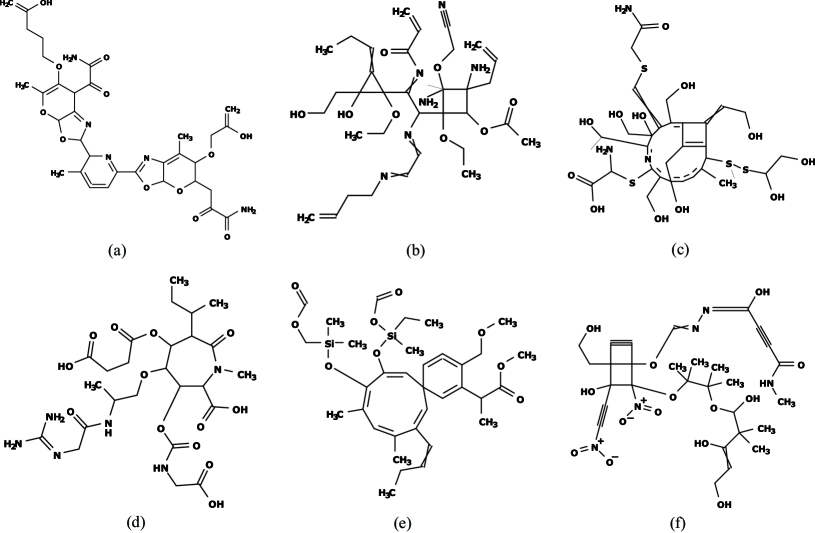
Figure 8: (a) $\mathbb{C}^{\dagger}$ with $\eta(f(\mathbb{C}^{\dagger}))=13703.3$ inferred from $I_{\mathrm{c}}$ with $(\underline{y}^{*},\overline{y}^{*})=(13700,13800)$ of Hc; (b) $\mathbb{C}^{\dagger}$ with $\eta(f(\mathbb{C}^{\dagger}))=21.62$ inferred from $I_{\mathrm{b}}^{2}$ with $(\underline{y}^{*},\overline{y}^{*})=(21,22)$ of Vd; (c) $\mathbb{C}^{\dagger}$ with $\eta(f(\mathbb{C}^{\dagger}))=70.9$ inferred from $I_{\mathrm{b}}^{4}$ with $(\underline{y}^{*},\overline{y}^{*})=(70,71)$ of OptR; (d) $\mathbb{C}^{\dagger}$ with $\eta(f(\mathbb{C}^{\dagger}))=1198.8$ inferred from $I_{\mathrm{d}}$ with $(\underline{y}^{*},\overline{y}^{*})=(1190,1210)$ of IhcLiq; (e) $\mathbb{C}^{\dagger}$ with $\eta(f(\mathbb{C}^{\dagger}))=1.880$ inferred from $I_{\mathrm{b}}^{3}$ with $(\underline{y}^{*},\overline{y}^{*})=(1.85,1.90)$ of Vis; (f) $\mathbb{C}^{\dagger}$ inferred from $I_{\mathrm{b}}^{4}$ with lower and upper bounds on the predicted property value $\eta_{\pi}(f(\mathbb{C}^{\dagger}))$ of property $\pi\in\{$Kow, Lp, Sl$\}$ in Table 7.

From Tables 2 to 6, we observe that an instance with a large number of variables and constraints takes more running time than those with a smaller size in general. In this experiment, we prepared several different types of instances: instances $I_{\mathrm{a}}$ and $I_{\mathrm{c}}$ have restricted seed graphs, the other instances have abstract seed graphs and instances $I_{\mathrm{c}}$ and $I_{\mathrm{d}}$ have restricted set of fringe-trees. All instances in this experiment are solved in a few seconds to around 30 seconds with our MILP formulation.

Inferring a chemical graph with target values in multiple properties Once we obtained prediction functions $\eta_{\pi}$ for several properties $\pi$, it is easy to include MILP formulations for these functions $\eta_{\pi}$ into a single MILP $\mathcal{M}(x,y;\mathcal{C}_{1})$ so as to infer a chemical graph that satisfies given target values $y^{*}$ for these properties at the same time. As an additional experiment in Stage 4, we inferred a chemical graph that has a desired predicted value each of three properties Kow, Lp and Sl, where we used the prediction function $\eta_{\pi}$ for each property $\pi\in\{$Kow, Lp, Sl$\}$ constructed in Stage 3. Table 7 shows the result of Stage 4 for inferring a chemical graph $\mathbb{C}^{\dagger}$ from instances $I_{\mathrm{b}}^{2}$, $I_{\mathrm{b}}^{3}$ and $I_{\mathrm{b}}^{4}$ with $\Lambda=\{{\tt H},{\tt C},{\tt N},{\tt O},{\tt S}_{(2)},{\tt S}_{(6)},{\tt Cl}\}$, where we denote the following:

1. $\pi$: one of the three properties Kow, Lp and Sl used in the experiment;

2. $\underline{y}^{*}_{\pi},~{}\overline{y}^{*}_{\pi}$: lower and upper bounds $\underline{y}^{*}_{\pi},\overline{y}^{*}_{\pi}\in\mathbb{R}$ on the predicted property value $\eta_{\pi}(f(\mathbb{C}^{\dagger}))$ of property $\pi\in\{$Kow, Lp, Sl$\}$ for a chemical graph $\mathbb{C}^{\dagger}$ to be inferred;

3. $\#$v (resp., $\#$c): the number of variables (resp., constraints) in the MILP in Stage 4;

4. I-time: the time (sec.) to solve the MILP in Stage 4;

5. $n$: the number $n(\mathbb{C}^{\dagger})$ of non-hydrogen atoms in the chemical graph $\mathbb{C}^{\dagger}$ inferred in Stage 4;

6. $\mathrm{n}^{\mathrm{int}}$: the number $\mathrm{n}^{\mathrm{int}}(\mathbb{C}^{\dagger})$ of interior-vertices in the chemical graph $\mathbb{C}^{\dagger}$ inferred in Stage 4; and

7. $\eta_{\pi}(f(\mathbb{C}^{\dagger}))$: the predicted property value $\eta_{\pi}(f(\mathbb{C}^{\dagger}))$ of property $\pi\in\{$Kow, Lp, Sl$\}$ for the chemical graph $\mathbb{C}^{\dagger}$ inferred in Stage 4.

Table 7: Results of Stage 4 for instance $I_{\mathrm{b}}^{i},i=2,3,4$ with specified target values of three properties Kow, Lp and Sl.

inst.	$\pi$	$\underline{y}_{\pi}^{*},~{}\overline{y}_{\pi}^{*}$	$\#$v	$\#$c	I-time	$n$	$\mathrm{n}^{\mathrm{int}}$	$\eta_{\pi}(f(\mathbb{C}^{\dagger}))$
	Kow	-7.50, -7.40						-7.41
$I_{\mathrm{b}}^{2}$	Lp	-1.40, -1.30	14574	11604	62.7	50	30	-1.33
	Sl	-11.6, -11.5						-11.52
	Kow	-7.40, -7.30						-7.38
$I_{\mathrm{b}}^{3}$	Lp	-2.90, -2.80	14370	11596	35.5	48	25	-2.81
	Sl	-11.6, -11.4						-11.52
	Kow	-7.50, -7.40						-7.48
$I_{\mathrm{b}}^{4}$	Lp	-0.70, -0.60	14166	11588	71.7	49	26	-0.63
	Sl	-11.4, -11.2						-11.39

Figure 8(f) illustrates the chemical graph $\mathbb{C}^{\dagger}$ inferred from $I_{\mathrm{b}}^{4}$ with $(\underline{y}^{*}_{\pi_{1}},\overline{y}^{*}_{\pi_{1}})=(-7.50,$ $-7.40)$, $(\underline{y}^{*}_{\pi_{2}},\overline{y}^{*}_{\pi_{2}})=(-0.70,-0.60)$ and $(\underline{y}^{*}_{\pi_{3}},\overline{y}^{*}_{\pi_{3}})=(-11.4,-11.2)$ for $\pi_{1}=$Kow, $\pi_{2}=$Lp and $\pi_{3}=$Sl, respectively.

Stage 5. We executed Stage 5 to generate a more number of target chemical graphs $\mathbb{C}^{*}$, where we call a chemical graph $\mathbb{C}^{*}$ a chemical isomer of a target chemical graph $\mathbb{C}^{\dagger}$ of a topological specification $\sigma$ if $f(\mathbb{C}^{*})=f(\mathbb{C}^{\dagger})$ and $\mathbb{C}^{*}$ also satisfies the same topological specification $\sigma$. We computed chemical isomers $\mathbb{C}^{*}$ of each target chemical graph $\mathbb{C}^{\dagger}$ inferred in Stage 4. We execute an algorithm for generating chemical isomers of $\mathbb{C}^{\dagger}$ up to 100 when the number of all chemical isomers exceeds 100. Such an algorithm can be obtained from the dynamic programming proposed by Tanaka et al. [26] with a slight modification. The algorithm first decomposes $\mathbb{C}^{\dagger}$ into a set of acyclic chemical graphs, next replaces each acyclic chemical graph $T$ with another acyclic chemical graph $T^{\prime}$ that admits the same feature vector as that of $T$, and finally assembles the resulting acyclic chemical graphs into a chemical isomer $\mathbb{C}^{*}$ of $\mathbb{C}^{\dagger}$. The algorithm can compute a lower bound on the total number of all chemical isomers of $\mathbb{C}^{\dagger}$ without generating all of them.

Tables 2 to 6 show the computational results of the experiment in Stage 5 for the five properties, where we denote the following:

1. D-time: the running time (sec.) to execute the dynamic programming algorithm in Stage 5 to compute a lower bound on the number of all chemical isomers $\mathbb{C}^{*}$ of $\mathbb{C}^{\dagger}$ and generate all (or up to 100) chemical isomers $\mathbb{C}^{*}$;

2. $\mathbb{C}$-LB: a lower bound on the number of all chemical isomers $\mathbb{C}^{*}$ of $\mathbb{C}^{\dagger}$; and

3. $\#\mathbb{C}$: the number of all (or up to 100) chemical isomers $\mathbb{C}^{*}$ of $\mathbb{C}^{\dagger}$ generated in Stage 5.

From Tables 2 to 6, we observe that the running time for generating up to 100 target chemical graphs in Stage 5 is less than 0.4 second for many cases. For some chemical graph $\mathbb{C}^{\dagger}$, no chemical isomer was found by our algorithm. This is because each acyclic chemical graph in the decomposition of $\mathbb{C}^{\dagger}$ has no alternative acyclic chemical graph than the original one. On the other hand, some chemical graph $\mathbb{C}^{\dagger}$ such as the one in $I_{\mathrm{d}}$ in Tables 2 admits extremely large number of chemical isomers $\mathbb{C}^{*}$. Remember that we know such a lower bound $\mathbb{C}$-LB on the number of chemical isomers without generating all of them.

6 Concluding Remarks

In the previous applications of the framework of inferring chemical graphs, artificial neural network (ANN) and decision tree have been used for the machine learning of Stage 3. In this paper, we used linear regression in Stage 3 for the first time and derived an MILP formulation that simulates the computation process of linear regression. We also extended a way of specifying a target value $y^{*}$ in a property so that the predicted value $\eta(f(\mathbb{C}^{\dagger}))$ of a target chemical graph $\mathbb{C}^{\dagger}$ is required to belong to an interval between two specified values $\underline{y}^{*}$ and $\overline{y}^{*}$. In this paper, we modified a model of chemical compounds so that multi-valence chemical elements, cation and anion are treated, and introduced the rank and the adjacency-configuration of leaf-edges as new descriptors in a feature vector of a chemical graph. We implemented the new system of the framework and conducted computational experiments for Stages 1 to 5. We found 18 properties for which linear regression delivers a relatively good prediction function by using our feature vector based on the two-layered model. We also observed that an MILP formulation for inferring a chemical graph in Stage 4 can be solved efficiently over different types of test instances with complicated topological specifications. The experimental result suggests that our method can infer chemical graphs with up to 50 non-hydrogen atoms.

It is left as a future work to use other learning methods such as random forest, graph convolution networks and an ensemble method in Stages 3 and 4 in the framework.

Appendix

Appendix A A Full Description of Descriptors

Associated with the two functions $\alpha$ and $\beta$ in a chemical graph $\mathbb{C}=(H,\alpha,\beta)$, we introduce functions $\mathrm{ac}:V(E)\to(\Lambda\setminus\{{\tt H}\})\times(\Lambda\setminus\{{\tt H}\})\times[1,3]$, $\mathrm{cs}:V(E)\to(\Lambda\setminus\{{\tt H}\})\times[1,6]$ and $\mathrm{ec}:V(E)\to((\Lambda\setminus\{{\tt H}\})\times[1,6])\times((\Lambda\setminus\{{\tt H}\})\times[1,6])\times[1,3]$ in the following.

To represent a feature of the exterior of $\mathbb{C}$, a chemical rooted tree in $\mathcal{T}(\mathbb{C})$ is called a fringe-configuration of $\mathbb{C}$.

We also represent leaf-edges in the exterior of $\mathbb{C}$. For a leaf-edge $uv\in E(\langle\mathbb{C}\rangle)$ with $\deg_{\langle\mathbb{C}\rangle}(u)=1$, we define the adjacency-configuration of $e$ to be an ordered tuple $(\alpha(u),\alpha(v),\beta(uv))$. Define

$$\Gamma_{\mathrm{ac}}^{\mathrm{lf}}\triangleq\{({\tt a},{\tt b},m)\mid{\tt a},{\tt b}\in\Lambda,m\in[1,\min\{\mathrm{val}({\tt a}),\mathrm{val}({\tt b})\}]\}$$

as a set of possible adjacency-configurations for leaf-edges.

To represent a feature of an interior-vertex $v\in V^{\mathrm{int}}(\mathbb{C})$ such that $\alpha(v)={\tt a}$ and $\deg_{\langle\mathbb{C}\rangle}(v)=d$ (i.e., the number of non-hydrogen atoms adjacent to $v$ is $d$) in a chemical graph $\mathbb{C}=(H,\alpha,\beta)$, we use a pair $({\tt a},d)\in(\Lambda\setminus\{{\tt H}\})\times[1,4]$, which we call the chemical symbol $\mathrm{cs}(v)$ of the vertex $v$. We treat $({\tt a},d)$ as a single symbol ${\tt a}d$, and define $\Lambda_{\mathrm{dg}}$ to be the set of all chemical symbols $\mu={\tt a}d\in(\Lambda\setminus\{{\tt H}\})\times[1,4]$.

We define a method for featuring interior-edges as follows. Let $e=uv\in E^{\mathrm{int}}(\mathbb{C})$ be an interior-edge $e=uv\in E^{\mathrm{int}}(\mathbb{C})$ such that $\alpha(u)={\tt a}$, $\alpha(v)={\tt b}$ and $\beta(e)=m$ in a chemical graph $\mathbb{C}=(H,\alpha,\beta)$. To feature this edge $e$, we use a tuple $({\tt a},{\tt b},m)\in(\Lambda\setminus\{{\tt H}\})\times(\Lambda\setminus\{{\tt H}\})\times[1,3]$, which we call the adjacency-configuration $\mathrm{ac}(e)$ of the edge $e$. We introduce a total order $<$ over the elements in $\Lambda$ to distinguish between $({\tt a},{\tt b},m)$ and $({\tt b},{\tt a},m)$ $({\tt a}\neq{\tt b})$ notationally. For a tuple $\nu=({\tt a},{\tt b},m)$, let $\overline{\nu}$ denote the tuple $({\tt b},{\tt a},m)$.

Let $e=uv\in E^{\mathrm{int}}(\mathbb{C})$ be an interior-edge $e=uv\in E^{\mathrm{int}}(\mathbb{C})$ such that $\mathrm{cs}(u)=\mu$, $\mathrm{cs}(v)=\mu^{\prime}$ and $\beta(e)=m$ in a chemical graph $\mathbb{C}=(H,\alpha,\beta)$. To feature this edge $e$, we use a tuple $(\mu,\mu^{\prime},m)\in\Lambda_{\mathrm{dg}}\times\Lambda_{\mathrm{dg}}\times[1,3]$, which we call the edge-configuration $\mathrm{ec}(e)$ of the edge $e$. We introduce a total order $<$ over the elements in $\Lambda_{\mathrm{dg}}$ to distinguish between $(\mu,\mu^{\prime},m)$ and $(\mu^{\prime},\mu,m)$ $(\mu\neq\mu^{\prime})$ notationally. For a tuple $\gamma=(\mu,\mu^{\prime},m)$, let $\overline{\gamma}$ denote the tuple $(\mu^{\prime},\mu,m)$.

Let $\pi$ be a chemical property for which we will construct a prediction function $\eta$ from a feature vector $f(\mathbb{C})$ of a chemical graph $\mathbb{C}$ to a predicted value $y\in\mathbb{R}$ for the chemical property of $\mathbb{C}$.

We first choose a set $\Lambda$ of chemical elements and then collect a data set $D_{\pi}$ of chemical compounds $C$ whose chemical elements belong to $\Lambda$, where we regard $D_{\pi}$ as a set of chemical graphs $\mathbb{C}$ that represent the chemical compounds $C$ in $D_{\pi}$. To define the interior/exterior of chemical graphs $\mathbb{C}\in D_{\pi}$, we next choose a branch-parameter ${\rho}$, where we recommend ${\rho}=2$.

Let $\Lambda^{\mathrm{int}}(D_{\pi})\subseteq\Lambda$ (resp., $\Lambda^{\mathrm{ex}}(D_{\pi})\subseteq\Lambda$) denote the set of chemical elements used in the set $V^{\mathrm{int}}(\mathbb{C})$ of interior-vertices (resp., the set $V^{\mathrm{ex}}(\mathbb{C})$ of exterior-vertices) of $\mathbb{C}$ over all chemical graphs $\mathbb{C}\in D_{\pi}$, and $\Gamma^{\mathrm{int}}(D_{\pi})$ denote the set of edge-configurations used in the set $E^{\mathrm{int}}(\mathbb{C})$ of interior-edges in $\mathbb{C}$ over all chemical graphs $\mathbb{C}\in D_{\pi}$. Let $\mathcal{F}(D_{\pi})$ denote the set of chemical rooted trees $\psi$ r-isomorphic to a chemical rooted tree in $\mathcal{T}(\mathbb{C})$ over all chemical graphs $\mathbb{C}\in D_{\pi}$, where possibly a chemical rooted tree $\psi\in\mathcal{F}(D_{\pi})$ consists of a single chemical element ${\tt a}\in\Lambda\setminus\{{\tt H}\}$.

We define an integer encoding of a finite set $A$ of elements to be a bijection $\sigma:A\to[1,|A|]$, where we denote by $[A]$ the set $[1,|A|]$ of integers. Introduce an integer coding of each of the sets $\Lambda^{\mathrm{int}}(D_{\pi})$, $\Lambda^{\mathrm{ex}}(D_{\pi})$, $\Gamma^{\mathrm{int}}(D_{\pi})$ and $\mathcal{F}(D_{\pi})$. Let $[{\tt a}]^{\mathrm{int}}$ (resp., $[{\tt a}]^{\mathrm{ex}}$) denote the coded integer of an element ${\tt a}\in\Lambda^{\mathrm{int}}(D_{\pi})$ (resp., ${\tt a}\in\Lambda^{\mathrm{ex}}(D_{\pi})$), $[\gamma]$ denote the coded integer of an element $\gamma$ in $\Gamma^{\mathrm{int}}(D_{\pi})$ and $[\psi]$ denote an element $\psi$ in $\mathcal{F}(D_{\pi})$.

Over 99% of chemical compounds $\mathbb{C}$ with up to 100 non-hydrogen atoms in PubChem have degree at most 4 in the hydrogen-suppressed graph $\langle\mathbb{C}\rangle$ [20]. We assume that a chemical graph $\mathbb{C}$ treated in this paper satisfies $\deg_{\langle\mathbb{C}\rangle}(v)\leq 4$ in the hydrogen-suppressed graph $\langle\mathbb{C}\rangle$.

In our model, we use an integer $\mathrm{mass}^{*}({\tt a})=\lfloor 10\cdot\mathrm{mass}({\tt a})\rfloor$, for each ${\tt a}\in\Lambda$.

We define the feature vector $f(\mathbb{C})$ of a chemical graph $\mathbb{C}=(H,\alpha,\beta)\in D_{\pi}$ to be a vector that consists of the following non-negative integer descriptors $\mathrm{dcp}_{i}(\mathbb{C})$, $i\in[1,K]$, where $K=14+|\Lambda^{\mathrm{int}}(D_{\pi})|+|\Lambda^{\mathrm{ex}}(D_{\pi})|+|\Gamma^{\mathrm{int}}(D_{\pi})|+|\mathcal{F}(D_{\pi})|+|\Gamma_{\mathrm{ac}}^{\mathrm{lf}}|$.

1. $\mathrm{dcp}_{1}(\mathbb{C})$: the number $|V(H)|-|V_{\tt H}|$ of non-hydrogen atoms in $\mathbb{C}$.

2. $\mathrm{dcp}_{2}(\mathbb{C})$: the rank $\mathrm{r}(\mathbb{C})$ of $\mathbb{C}$.

3. $\mathrm{dcp}_{3}(\mathbb{C})$: the number $|V^{\mathrm{int}}(\mathbb{C})|$ of interior-vertices in $\mathbb{C}$.

4. $\mathrm{dcp}_{4}(\mathbb{C})$: the average $\overline{\mathrm{ms}}(\mathbb{C})$ of mass^∗ over all atoms in $\mathbb{C}$;
   i.e., $\overline{\mathrm{ms}}(\mathbb{C})\triangleq\frac{1}{|V(H)|}\sum_{v\in V(H)}\mathrm{mass}^{*}(\alpha(v))$.

5. $\mathrm{dcp}_{i}(\mathbb{C})$, $i=4+d,d\in[1,4]$: the number $\mathrm{dg}_{d}^{\overline{{\tt H}}}(\mathbb{C})$ of non-hydrogen vertices $v\in V(H)\setminus V_{\tt H}$ of degree $\deg_{\langle\mathbb{C}\rangle}(v)=d$ in the hydrogen-suppressed chemical graph $\langle\mathbb{C}\rangle$.

6. $\mathrm{dcp}_{i}(\mathbb{C})$, $i=8+d,d\in[1,4]$: the number $\mathrm{dg}_{d}^{\mathrm{int}}(\mathbb{C})$ of interior-vertices of interior-degree $\deg_{\mathbb{C}^{\mathrm{int}}}(v)=d$ in the interior $\mathbb{C}^{\mathrm{int}}=(V^{\mathrm{int}}(\mathbb{C}),E^{\mathrm{int}}(\mathbb{C}))$ of $\mathbb{C}$.

7. $\mathrm{dcp}_{i}(\mathbb{C})$, $i=12+m$, $m\in[2,3]$: the number $\mathrm{bd}_{m}^{\mathrm{int}}(\mathbb{C})$ of interior-edges with bond multiplicity $m$ in $\mathbb{C}$; i.e., $\mathrm{bd}_{m}^{\mathrm{int}}(\mathbb{C})\triangleq\{e\in E^{\mathrm{int}}(\mathbb{C})\mid\beta(e)=m\}$.

8. $\mathrm{dcp}_{i}(\mathbb{C})$, $i=14+[{\tt a}]^{\mathrm{int}}$, ${\tt a}\in\Lambda^{\mathrm{int}}(D_{\pi})$: the frequency $\mathrm{na}_{\tt a}^{\mathrm{int}}(\mathbb{C})=|V_{\tt a}(\mathbb{C})\cap V^{\mathrm{int}}(\mathbb{C})|$ of chemical element ${\tt a}$ in the set $V^{\mathrm{int}}(\mathbb{C})$ of interior-vertices in $\mathbb{C}$.

9. $\mathrm{dcp}_{i}(\mathbb{C})$, $i=14+|\Lambda^{\mathrm{int}}(D_{\pi})|+[{\tt a}]^{\mathrm{ex}}$, ${\tt a}\in\Lambda^{\mathrm{ex}}(D_{\pi})$: the frequency $\mathrm{na}_{\tt a}^{\mathrm{ex}}(\mathbb{C})=|V_{\tt a}(\mathbb{C})\cap V^{\mathrm{ex}}(\mathbb{C})|$ of chemical element ${\tt a}$ in the set $V^{\mathrm{ex}}(\mathbb{C})$ of exterior-vertices in $\mathbb{C}$.

10. $\mathrm{dcp}_{i}(\mathbb{C})$, $i=14+|\Lambda^{\mathrm{int}}(D_{\pi})|+|\Lambda^{\mathrm{ex}}(D_{\pi})|+[\gamma]$, $\gamma\in\Gamma^{\mathrm{int}}(D_{\pi})$: the frequency $\mathrm{ec}_{\gamma}(\mathbb{C})$ of edge-configuration $\gamma$ in the set $E^{\mathrm{int}}(\mathbb{C})$ of interior-edges in $\mathbb{C}$.

11. $\mathrm{dcp}_{i}(\mathbb{C})$, $i=14+|\Lambda^{\mathrm{int}}(D_{\pi})|+|\Lambda^{\mathrm{ex}}(D_{\pi})|+|\Gamma^{\mathrm{int}}(D_{\pi})|+[\psi]$, $\psi\in\mathcal{F}(D_{\pi})$: the frequency $\mathrm{fc}_{\psi}(\mathbb{C})$ of fringe-configuration $\psi$ in the set of ${\rho}$-fringe-trees in $\mathbb{C}$.

12. $\mathrm{dcp}_{i}(\mathbb{C})$, $i=14+|\Lambda^{\mathrm{int}}(D_{\pi})|+|\Lambda^{\mathrm{ex}}(D_{\pi})|+|\Gamma^{\mathrm{int}}(D_{\pi})|+|\mathcal{F}(D_{\pi})|+[\nu]$, $\nu\in\Gamma_{\mathrm{ac}}^{\mathrm{lf}}$: the frequency $\mathrm{ac}_{\nu}^{\mathrm{lf}}(\mathbb{C})$ of adjacency-configuration $\nu$ in the set of leaf-edges in $\langle\mathbb{C}\rangle$.

Appendix B Specifying Target Chemical Graphs

Given a prediction function $\eta$ and a target value $y^{*}\in\mathbb{R}$, we call a chemical graph $\mathbb{C}^{*}$ such that $\eta(x^{*})=y^{*}$ for the feature vector $x^{*}=f(\mathbb{C}^{*})$ a target chemical graph. This section presents a set of rules for specifying topological substructure of a target chemical graph in a flexible way in Stage 4.

We first describe how to reduce a chemical graph $\mathbb{C}=(H,\alpha,\beta)$ into an abstract form based on which our specification rules will be defined. To illustrate the reduction process, we use the chemical graph $\mathbb{C}=(H,\alpha,\beta)$ such that $\langle\mathbb{C}\rangle$ is given in Figure 2.

1. Removal of all ${\rho}$-fringe-trees: The interior $H^{\mathrm{int}}=(V^{\mathrm{int}}(\mathbb{C}),E^{\mathrm{int}}(\mathbb{C}))$ of $\mathbb{C}$ is obtained by removing the non-root vertices of each ${\rho}$-fringe-trees $\mathbb{C}[u]\in\mathcal{T}(\mathbb{C}),u\in V^{\mathrm{int}}(\mathbb{C})$. Figure 9 illustrates the interior $H^{\mathrm{int}}$ of chemical graph $\mathbb{C}$ with ${\rho}=2$ in Figure 2.

2. Removal of some leaf paths: We call a $u,v$-path $Q$ in $H^{\mathrm{int}}$ a leaf path if vertex $v$ is a leaf-vertex of $H^{\mathrm{int}}$ and the degree of each internal vertex of $Q$ in $H^{\mathrm{int}}$ is 2, where we regard that $Q$ is rooted at vertex $u$. A connected subgraph $S$ of the interior $H^{\mathrm{int}}$ of $\mathbb{C}$ is called a cyclical-base if $S$ is obtained from $H$ by removing the vertices in $V(Q_{u})\setminus\{u\},u\in X$ for a subset $X$ of interior-vertices and a set $\{Q_{u}\mid u\in X\}$ of leaf $u,v$-paths $Q_{u}$ such that no two paths $Q_{u}$ and $Q_{u^{\prime}}$ share a vertex. Figure 10(a) illustrates a cyclical-base $S=H^{\mathrm{int}}-\bigcup_{u\in X}(V(Q_{u})\setminus\{u\})$ of the interior $H^{\mathrm{int}}$ for a set $\{Q_{u_{5}}=(u_{5},u_{24}),Q_{u_{18}}=(u_{18},u_{25},u_{26},u_{27}),Q_{u_{22}}=(u_{22},u_{28})\}$ of leaf paths in Figure 9.

3. Contraction of some pure paths: A path in $S$ is called pure if each internal vertex of the path is of degree 2. Choose a set $\mathcal{P}$ of several pure paths in $S$ so that no two paths share vertices except for their end-vertices. A graph $S^{\prime}$ is called a contraction of a graph $S$ (with respect to $\mathcal{P}$) if $S^{\prime}$ is obtained from $S$ by replacing each pure $u,v$-path with a single edge $a=uv$, where $S^{\prime}$ may contain multiple edges between the same pair of adjacent vertices. Figure 10(b) illustrates a contraction $S^{\prime}$ obtained from the chemical graph $S$ by contracting each $uv$-path $P_{a}\in\mathcal{P}$ into a new edge $a=uv$, where $a_{1}=u_{1}u_{2},a_{2}=u_{1}u_{3},a_{3}=u_{4}u_{7},a_{4}=u_{10}u_{11}$ and $a_{5}=u_{11}u_{12}$ and $\mathcal{P}=\{P_{a_{1}}=(u_{1},u_{13},u_{2}),P_{a_{2}}=(u_{1},u_{14},u_{3}),P_{a_{3}}=(u_{4},u_{15},u_{16},u_{7}),P_{a_{4}}=(u_{10},u_{17},u_{18},u_{19},u_{11}),P_{a_{5}}=(u_{11},u_{20},u_{21},u_{22},u_{12})\}$ of pure paths in Figure 10(a).

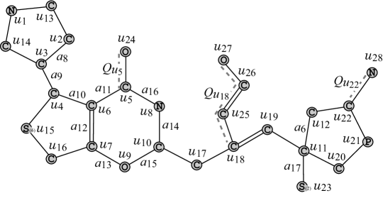
Figure 9: The interior $H^{\mathrm{int}}$ of chemical graph $\mathbb{C}$ with $\langle\mathbb{C}\rangle$ in Figure 2 for ${\rho}=2$.

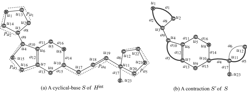
Figure 10: (a) A cyclical-base $S=H^{\mathrm{int}}-\bigcup_{u\in\{u_{5},u_{18},u_{22}\}}(V(Q_{u})\setminus\{u\})$ of the interior $H^{\mathrm{int}}$ in Figure 9; (b) A contraction $S^{\prime}$ of $S$ for a pure path set $\mathcal{P}=\{P_{a_{1}},P_{a_{2}},\ldots,P_{a_{5}}\}$ in (a), where a new edge obtained by contracting a pure path is depicted with a thick line.

We will define a set of rules so that a chemical graph can be obtained from a graph (called a seed graph in the next section) by applying processes R3 to R1 in a reverse way. We specify topological substructures of a target chemical graph with a tuple $(G_{\mathrm{C}},\sigma_{\mathrm{int}},\sigma_{\mathrm{ce}})$ called a target specification defined under the set of the following rules.

Seed Graph

A seed graph $G_{\mathrm{C}}=(V_{\mathrm{C}},E_{\mathrm{C}})$ is defined to be a graph (possibly with multiple edges) such that the edge set $E_{\mathrm{C}}$ consists of four sets $E_{(\geq 2)}$, $E_{(\geq 1)}$, $E_{(0/1)}$ and $E_{(=1)}$, where each of them can be empty. A seed graph plays a role of the most abstract form $S^{\prime}$ in R3. Figure 4(a) illustrates an example of a seed graph $G_{\mathrm{C}}$ with $\mathrm{r}(G_{\mathrm{C}})=5$, where $V_{\mathrm{C}}=\{u_{1},u_{2},\ldots,u_{12},u_{23}\}$, $E_{(\geq 2)}=\{a_{1},a_{2},\ldots,a_{5}\}$, $E_{(\geq 1)}=\{a_{6}\}$, $E_{(0/1)}=\{a_{7}\}$ and $E_{(=1)}=\{a_{8},a_{9},\ldots,a_{16}\}$.

A subdivision $S$ of $G_{\mathrm{C}}$ is a graph constructed from a seed graph $G_{\mathrm{C}}$ according to the following rules:

1. Each edge $e=uv\in E_{(\geq 2)}$ is replaced with a $u,v$-path $P_{e}$ of length at least 2;

2. Each edge $e=uv\in E_{(\geq 1)}$ is replaced with a $u,v$-path $P_{e}$ of length at least 1 (equivalently $e$ is directly used or replaced with a $u,v$-path $P_{e}$ of length at least 2);

3. Each edge $e\in E_{(0/1)}$ is either used or discarded, where $E_{(0/1)}$ is required to be chosen as a non-separating edge subset of $E(G_{\mathrm{C}})$ since otherwise the connectivity of a final chemical graph $\mathbb{C}$ is not guaranteed; $\mathrm{r}(\mathbb{C})=\mathrm{r}(G_{\mathrm{C}})-|E^{\prime}|$ holds for a subset $E^{\prime}\subseteq E_{(0/1)}$ of edges discarded in a final chemical graph $\mathbb{C}$; and

4. Each edge $e\in E_{(=1)}$ is always used directly.

We allow a possible elimination of edges in $E_{(0/1)}$ as an optional rule in constructing a target chemical graph from a seed graph, even though such an operation has not been included in the process R3. A subdivision $S$ plays a role of a cyclical-base in R2. A target chemical graph $\mathbb{C}=(H,\alpha,\beta)$ will contain $S$ as a subgraph of the interior $H^{\mathrm{int}}$ of $\mathbb{C}$.

Interior-specification

A graph $H^{*}$ that serves as the interior $H^{\mathrm{int}}$ of a target chemical graph $\mathbb{C}$ will be constructed as follows. First construct a subdivision $S$ of a seed graph $G_{\mathrm{C}}$ by replacing each edge $e=uu^{\prime}\in E_{(\geq 2)}\cup E_{(\geq 1)}$ with a pure $u,u^{\prime}$-path $P_{e}$. Next construct a supergraph $H^{*}$ of $S$ by attaching a leaf path $Q_{v}$ at each vertex $v\in V_{\mathrm{C}}$ or at an internal vertex $v\in V(P_{e})\setminus\{u,u^{\prime}\}$ of each pure $u,u^{\prime}$-path $P_{e}$ for some edge $e=uu^{\prime}\in E_{(\geq 2)}\cup E_{(\geq 1)}$, where possibly $Q_{v}=(v),E(Q_{v})=\emptyset$ (i.e., we do not attach any new edges to $v$). We introduce the following rules for specifying the size of $H^{*}$, the length $|E(P_{e})|$ of a pure path $P_{e}$, the length $|E(Q_{v})|$ of a leaf path $Q_{v}$, the number of leaf paths $Q_{v}$ and a bond-multiplicity of each interior-edge, where we call the set of prescribed constants an interior-specification $\sigma_{\mathrm{int}}$:

1. Lower and upper bounds $\mathrm{n}^{\mathrm{int}}_{\mathrm{LB}},\mathrm{n}^{\mathrm{int}}_{\mathrm{UB}}\in\mathbb{Z}_{+}$ on the number of interior-vertices of a target chemical graph $\mathbb{C}$.

2. For each edge $e=uu^{\prime}\in E_{(\geq 2)}\cup E_{(\geq 1)}$,

   a lower bound $\ell_{\mathrm{LB}}(e)$ and an upper bound $\ell_{\mathrm{UB}}(e)$ on the length $|E(P_{e})|$ of a pure $u,u^{\prime}$-path $P_{e}$. (For a notational convenience, set $\ell_{\mathrm{LB}}(e):=0$, $\ell_{\mathrm{UB}}(e):=1$, $e\in E_{(0/1)}$ and $\ell_{\mathrm{LB}}(e):=1$, $\ell_{\mathrm{UB}}(e):=1$, $e\in E_{(=1)}$.)

   a lower bound $\mathrm{bl}_{\mathrm{LB}}(e)$ and an upper bound $\mathrm{bl}_{\mathrm{UB}}(e)$ on the number of leaf paths $Q_{v}$ attached at internal vertices $v$ of a pure $u,u^{\prime}$-path $P_{e}$.

   a lower bound $\mathrm{ch}_{\mathrm{LB}}(e)$ and an upper bound $\mathrm{ch}_{\mathrm{UB}}(e)$ on the maximum length $|E(Q_{v})|$ of a leaf path $Q_{v}$ attached at an internal vertex $v\in V(P_{e})\setminus\{u,u^{\prime}\}$ of a pure $u,u^{\prime}$-path $P_{e}$.

3. For each vertex $v\in V_{\mathrm{C}}$,

   a lower bound $\mathrm{ch}_{\mathrm{LB}}(v)$ and an upper bound $\mathrm{ch}_{\mathrm{UB}}(v)$ on the number of leaf paths $Q_{v}$ attached to $v$, where $0\leq\mathrm{ch}_{\mathrm{LB}}(v)\leq\mathrm{ch}_{\mathrm{UB}}(v)\leq 1$.

   a lower bound $\mathrm{ch}_{\mathrm{LB}}(v)$ and an upper bound $\mathrm{ch}_{\mathrm{UB}}(v)$ on the length $|E(Q_{v})|$ of a leaf path $Q_{v}$ attached to $v$.

4. For each edge $e=uu^{\prime}\in E_{\mathrm{C}}$, a lower bound $\mathrm{bd}_{m,\mathrm{LB}}(e)$ and an upper bound $\mathrm{bd}_{m,\mathrm{UB}}(e)$ on the number of edges with bond-multiplicity $m\in[2,3]$ in $u,u^{\prime}$-path $P_{e}$, where we regard $P_{e}$, $e\in E_{(0/1)}\cup E_{(=1)}$ as single edge $e$.

We call a graph $H^{*}$ that satisfies an interior-specification $\sigma_{\mathrm{int}}$ a $\sigma_{\mathrm{int}}$-extension of $G_{\mathrm{C}}$, where the bond-multiplicity of each edge has been determined.

Table 8 shows an example of an interior-specification $\sigma_{\mathrm{int}}$ to the seed graph $G_{\mathrm{C}}$ in Figure 4.

Table 8: Example 1 of an interior-specification $\sigma_{\mathrm{int}}$.

$\mathrm{n}^{\mathrm{int}}_{\mathrm{LB}}=20$

$\mathrm{n}^{\mathrm{int}}_{\mathrm{UB}}=28$

	$a_{1}$	$a_{2}$	$a_{3}$	$a_{4}$	$a_{5}$	$a_{6}$
$\ell_{\mathrm{LB}}(a_{i})$	2	2	2	3	2	1
$\ell_{\mathrm{UB}}(a_{i})$	3	4	3	5	4	4
$\mathrm{bl}_{\mathrm{LB}}(a_{i})$	0	0	0	1	1	0
$\mathrm{bl}_{\mathrm{UB}}(a_{i})$	1	1	0	2	1	0
$\mathrm{ch}_{\mathrm{LB}}(a_{i})$	0	1	0	4	3	0
$\mathrm{ch}_{\mathrm{UB}}(a_{i})$	3	3	1	6	5	2

	$u_{1}$	$u_{2}$	$u_{3}$	$u_{4}$	$u_{5}$	$u_{6}$	$u_{7}$	$u_{8}$	$u_{9}$	$u_{10}$	$u_{11}$	$u_{12}$	$u_{23}$
$\mathrm{bl}_{\mathrm{LB}}(u_{i})$	0	0	0	0	0	0	0	0	0	0	0	0	0
$\mathrm{bl}_{\mathrm{UB}}(u_{i})$	1	1	1	1	1	0	0	0	0	0	0	0	0
$\mathrm{ch}_{\mathrm{LB}}(u_{i})$	0	0	0	0	1	0	0	0	0	0	0	0	0
$\mathrm{ch}_{\mathrm{UB}}(u_{i})$	1	0	0	0	3	0	1	1	0	1	2	4	1

	$a_{1}$	$a_{2}$	$a_{3}$	$a_{4}$	$a_{5}$	$a_{6}$	$a_{7}$	$a_{8}$	$a_{9}$	$a_{10}$	$a_{11}$	$a_{12}$	$a_{13}$	$a_{14}$	$a_{15}$	$a_{16}$	$a_{17}$
$\mathrm{bd}_{2,\mathrm{LB}}(a_{i})$	0	0	0	1	0	0	0	0	0	0	0	1	0	0	0	0	0
$\mathrm{bd}_{2,\mathrm{UB}}(a_{i})$	1	1	0	2	2	0	0	0	0	0	0	1	0	0	0	0	0
$\mathrm{bd}_{3,\mathrm{LB}}(a_{i})$	0	0	0	0	0	0	0	0	0	0	0	0	0	0	0	0	0
$\mathrm{bd}_{3,\mathrm{UB}}(a_{i})$	0	0	0	0	1	0	0	0	0	0	0	0	0	0	0	0	0

Figure 11 illustrates an example of an $\sigma_{\mathrm{int}}$-extension $H^{*}$ of seed graph $G_{\mathrm{C}}$ in Figure 4 under the interior-specification $\sigma_{\mathrm{int}}$ in Table 8.

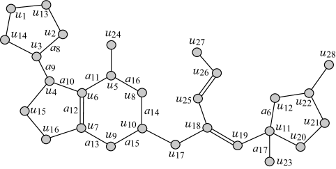
Figure 11: An illustration of a graph $H^{*}$ that is obtained from the seed graph $G_{\mathrm{C}}$ in Figure 4 under the interior-specification $\sigma_{\mathrm{int}}$ in Table 8, where the vertices newly introduced by pure paths $P_{a_{i}}$ and leaf paths $Q_{v_{i}}$ are depicted with white squares and circles, respectively.

Chemical-specification

Let $H^{*}$ be a graph that serves as the interior $H^{\mathrm{int}}$ of a target chemical graph $\mathbb{C}$, where the bond-multiplicity of each edge in $H^{*}$ has be determined. Finally we introduce a set of rules for constructing a target chemical graph $\mathbb{C}$ from $H^{*}$ by choosing a chemical element ${\tt a}\in\Lambda$ and assigning a ${\rho}$-fringe-tree $\psi$ to each interior-vertex $v\in V^{\mathrm{int}}$. We introduce the following rules for specifying the size of $\mathbb{C}$, a set of chemical rooted trees that are allowed to use as ${\rho}$-fringe-trees and lower and upper bounds on the frequency of a chemical element, a chemical symbol, and an edge-configuration, where we call the set of prescribed constants a chemical specification $\sigma_{\mathrm{ce}}$:

1. Lower and upper bounds $n_{\mathrm{LB}},n^{*}\in\mathbb{Z}_{+}$ on the number of vertices, where $\mathrm{n}^{\mathrm{int}}_{\mathrm{LB}}\leq n_{\mathrm{LB}}\leq n^{*}$.

2. Subsets $\mathcal{F}(v)\subseteq\mathcal{F}(D_{\pi}),v\in V_{\mathrm{C}}$ and $\mathcal{F}_{E}\subseteq\mathcal{F}(D_{\pi})$ of chemical rooted trees $\psi$ with $\mathrm{ht}(\langle\psi\rangle)\leq{\rho}$, where we require that every ${\rho}$-fringe-tree $\mathbb{C}[v]$ rooted at a vertex $v\in V_{\mathrm{C}}$ (resp., at an internal vertex $v$ not in $V_{\mathrm{C}}$) in $\mathbb{C}$ belongs to $\mathcal{F}(v)$ (resp., $\mathcal{F}_{E}$). Let $\mathcal{F}^{*}:=\mathcal{F}_{E}\cup\bigcup_{v\in V_{\mathrm{C}}}\mathcal{F}(v)$ and $\Lambda^{\mathrm{ex}}$ denote the set of chemical elements assigned to non-root vertices over all chemical rooted trees in $\mathcal{F}^{*}$.

3. A subset $\Lambda^{\mathrm{int}}\subseteq\Lambda^{\mathrm{int}}(D_{\pi})$, where we require that every chemical element $\alpha(v)$ assigned to an interior-vertex $v$ in $\mathbb{C}$ belongs to $\Lambda^{\mathrm{int}}$. Let $\Lambda:=\Lambda^{\mathrm{int}}\cup\Lambda^{\mathrm{ex}}$ and $\mathrm{na}_{\tt a}(\mathbb{C})$ (resp., $\mathrm{na}_{\tt a}^{\mathrm{int}}(\mathbb{C})$ and $\mathrm{na}_{\tt a}^{\mathrm{ex}}(\mathbb{C})$) denote the number of vertices (resp., interior-vertices and exterior-vertices) $v$ such that $\alpha(v)={\tt a}$ in $\mathbb{C}$.

4. A set $\Lambda_{\mathrm{dg}}^{\mathrm{int}}\subseteq\Lambda\times[1,4]$ of chemical symbols and a set $\Gamma^{\mathrm{int}}\subseteq\Gamma^{\mathrm{int}}(D_{\pi})$ of edge-configurations $(\mu,\mu^{\prime},m)$ with $\mu\leq\mu^{\prime}$, where we require that the edge-configuration $\mathrm{ec}(e)$ of an interior-edge $e$ in $\mathbb{C}$ belongs to $\Gamma^{\mathrm{int}}$. We do not distinguish $(\mu,\mu^{\prime},m)$ and $(\mu^{\prime},\mu,m)$.

5. Define $\Gamma_{\mathrm{ac}}^{\mathrm{int}}$ to be the set of adjacency-configurations such that $\Gamma_{\mathrm{ac}}^{\mathrm{int}}:=\{({\tt a},{\tt b},m)\mid({\tt a}d,{\tt b}d^{\prime},m)\in\Gamma^{\mathrm{int}}\}$. Let $\mathrm{ac}_{\nu}^{\mathrm{int}}(\mathbb{C}),\nu\in\Gamma_{\mathrm{ac}}^{\mathrm{int}}$ denote the number of interior-edges $e$ such that $\mathrm{ac}(e)=\nu$ in $\mathbb{C}$.

6. Subsets $\Lambda^{*}(v)\subseteq\{{\tt a}\in\Lambda^{\mathrm{int}}\mid\mathrm{val}({\tt a})\geq 2\}$, $v\in V_{\mathrm{C}}$, we require that every chemical element $\alpha(v)$ assigned to a vertex $v\in V_{\mathrm{C}}$ in the seed graph belongs to $\Lambda^{*}(v)$.

7. Lower and upper bound functions $\mathrm{na}_{\mathrm{LB}},\mathrm{na}_{\mathrm{UB}}:\Lambda\to[1,n^{*}]$ and $\mathrm{na}_{\mathrm{LB}}^{\mathrm{int}},\mathrm{na}_{\mathrm{UB}}^{\mathrm{int}}:\Lambda^{\mathrm{int}}\to[1,n^{*}]$ on the number of interior-vertices $v$ such that $\alpha(v)={\tt a}$ in $\mathbb{C}$.

8. Lower and upper bound functions $\mathrm{ns}_{\mathrm{LB}}^{\mathrm{int}},\mathrm{ns}_{\mathrm{UB}}^{\mathrm{int}}:\Lambda_{\mathrm{dg}}^{\mathrm{int}}\to[1,n^{*}]$ on the number of interior-vertices $v$ such that $\mathrm{cs}(v)=\mu$ in $\mathbb{C}$.

9. Lower and upper bound functions $\mathrm{ac}_{\mathrm{LB}}^{\mathrm{int}},\mathrm{ac}_{\mathrm{UB}}^{\mathrm{int}}:\Gamma_{\mathrm{ac}}^{\mathrm{int}}\to\mathbb{Z}_{+}$ on the number of interior-edges $e$ such that $\mathrm{ac}(e)=\nu$ in $\mathbb{C}$.

10. Lower and upper bound functions $\mathrm{ec}_{\mathrm{LB}}^{\mathrm{int}},\mathrm{ec}_{\mathrm{UB}}^{\mathrm{int}}:\Gamma^{\mathrm{int}}\to\mathbb{Z}_{+}$ on the number of interior-edges $e$ such that $\mathrm{ec}(e)=\gamma$ in $\mathbb{C}$.

11. Lower and upper bound functions $\mathrm{fc}_{\mathrm{LB}},\mathrm{fc}_{\mathrm{UB}}:\mathcal{F}^{*}\to[0,n^{*}]$ on the number of interior-vertices $v$ such that $\mathbb{C}[v]$ is r-isomorphic to $\psi\in\mathcal{F}^{*}$ in $\mathbb{C}$.

12. Lower and upper bound functions $\mathrm{ac}^{\mathrm{lf}}_{\mathrm{LB}},\mathrm{ac}^{\mathrm{lf}}_{\mathrm{UB}}:\Gamma_{\mathrm{ac}}^{\mathrm{lf}}\to[0,n^{*}]$ on the number of leaf-edges $uv$ in $\mathrm{ac}_{\mathrm{C}}$ with adjacency-configuration $\nu$.

We call a chemical graph $\mathbb{C}$ that satisfies a chemical specification $\sigma_{\mathrm{ce}}$ a $(\sigma_{\mathrm{int}},\sigma_{\mathrm{ce}})$-extension of $G_{\mathrm{C}}$, and denote by $\mathcal{G}(G_{\mathrm{C}},\sigma_{\mathrm{int}},\sigma_{\mathrm{ce}})$ the set of all $(\sigma_{\mathrm{int}},\sigma_{\mathrm{ce}})$-extensions of $G_{\mathrm{C}}$.

Table 9 shows an example of a chemical-specification $\sigma_{\mathrm{ce}}$ to the seed graph $G_{\mathrm{C}}$ in Figure 4.

Table 9: Example 2 of a chemical-specification $\sigma_{\mathrm{ce}}$.

$n_{\mathrm{LB}}=30$, $n^{*}=50$.

branch-parameter: ${\rho}=2$

Each of sets $\mathcal{F}(v),v\in V_{\mathrm{C}}$ and $\mathcal{F}_{E}$ is set to be

the set $\mathcal{F}$ of chemical rooted trees $\psi$ with $\mathrm{ht}(\langle\psi\rangle)\leq{\rho}=2$ in Figure 4(b).

$\Lambda=\{{\tt H},{\tt C},{\tt N},{\tt O},{\tt S}_{(2)},{\tt S}_{(6)},{\tt P}={\tt P}_{(5)}\}$

$\Lambda_{\mathrm{dg}}^{\mathrm{int}}=\{{\tt C}2,{\tt C}3,{\tt C}4,{\tt N}2,{\tt N}3,{\tt O}2,{\tt S}_{(2)}2,{\tt S}_{(6)}3,{\tt P}4\}$

$\Gamma_{\mathrm{ac}}^{\mathrm{int}}$

$\nu_{1}\!=\!({\tt C},{\tt C},1),\nu_{2}\!=\!({\tt C},{\tt C},2),\nu_{3}\!=\!({\tt C},{\tt N},1),\nu_{4}\!=\!({\tt C},{\tt O},1),\nu_{5}\!=\!({\tt C},{\tt S}_{(2)},1),\nu_{6}\!=\!({\tt C},{\tt S}_{(6)},1),\nu_{7}\!=\!({\tt C},{\tt P},1)$

$\Gamma^{\mathrm{int}}$	$\gamma_{1}\!=\!({\tt C}2,{\tt C}2,1),\gamma_{2}\!=\!({\tt C}2,{\tt C}3,1),\gamma_{3}\!=\!({\tt C}2,{\tt C}3,2),\gamma_{4}\!=\!({\tt C}2,{\tt C}4,1),\gamma_{5}\!=\!({\tt C}3,{\tt C}3,1),\gamma_{6}\!=\!({\tt C}3,{\tt C}3,2),$
	$\gamma_{7}\!=\!({\tt C}3,{\tt C}4,1),\gamma_{8}\!=\!({\tt C}2,{\tt N}2,1),\gamma_{9}\!=\!({\tt C}3,{\tt N}2,1),\gamma_{10}\!=\!({\tt C}3,{\tt O}2,1),\gamma_{11}\!=\!({\tt C}2,{\tt C}2,2),\gamma_{12}\!=\!({\tt C}2,{\tt O}2,1),$
	$\gamma_{13}\!=\!({\tt C}3,{\tt N}3,1),\gamma_{14}\!=\!({\tt C}4,{\tt S}_{(2)}2,2),\gamma_{15}\!=\!({\tt C}2,{\tt S}_{(6)}3,1),\gamma_{16}\!=\!({\tt C}3,{\tt S}_{\tiny(6)}3,1),\gamma_{17}\!=\!({\tt C}2,{\tt P}4,2),$
	$\gamma_{18}\!=\!({\tt C}3,{\tt P}4,1)$

$\Lambda^{*}(u_{1})=\Lambda^{*}(u_{8})=\{{\tt C,N}\}$, $\Lambda^{*}(u_{9})=\{{\tt C,O}\}$, $\Lambda^{*}(u)=\{{\tt C}\}$, $u\in V_{\mathrm{C}}\setminus\{u_{1},u_{8},u_{9}\}$

	${\tt H}$	${\tt C}$	${\tt N}$	${\tt O}$	${\tt S}_{(2)}$	${\tt S}_{(6)}$	${\tt P}$
$\mathrm{na}_{\mathrm{LB}}({\tt a})$	40	27	1	1	0	0	0
$\mathrm{na}_{\mathrm{UB}}({\tt a})$	65	37	4	8	1	1	1

	${\tt C}$	${\tt N}$	${\tt O}$	${\tt S}_{(2)}$	${\tt S}_{(6)}$	${\tt P}$
$\mathrm{na}_{\mathrm{LB}}^{\mathrm{int}}({\tt a})$	9	1	0	0	0	0
$\mathrm{na}_{\mathrm{UB}}^{\mathrm{int}}({\tt a})$	23	4	5	1	1	1

	${\tt C}2$	${\tt C}3$	${\tt C}4$	${\tt N}2$	${\tt N}3$	${\tt O}2$	${\tt S}_{(2)}2$	${\tt S}_{(6)}3$	${\tt P}4$
$\mathrm{ns}_{\mathrm{LB}}^{\mathrm{int}}(\mu)$	3	5	0	0	0	0	0	0	0
$\mathrm{ns}_{\mathrm{UB}}^{\mathrm{int}}(\mu)$	8	15	2	2	3	5	1	1	1

	$\nu_{1}$	$\nu_{2}$	$\nu_{3}$	$\nu_{4}$	$\nu_{5}$	$\nu_{6}$	$\nu_{7}$
$\mathrm{ac}_{\mathrm{LB}}^{\mathrm{int}}(\nu)$	0	0	0	0	0	0	0
$\mathrm{ac}_{\mathrm{UB}}^{\mathrm{int}}(\nu)$	30	10	10	10	1	1	1

	$\gamma_{1}$	$\gamma_{2}$	$\gamma_{3}$	$\gamma_{4}$	$\gamma_{5}$	$\gamma_{6}$	$\gamma_{7}$	$\gamma_{8}$	$\gamma_{9}$	$\gamma_{10}$	$\gamma_{11}$	$\gamma_{12}$	$\gamma_{13}$	$\gamma_{14}$	$\gamma_{15}$	$\gamma_{16}$	$\gamma_{17}$	$\gamma_{18}$
$\mathrm{ec}_{\mathrm{LB}}^{\mathrm{int}}(\gamma)$	0	0	0	0	0	0	0	0	0	0	0	0	0	0	0	0	0	0
$\mathrm{ec}_{\mathrm{UB}}^{\mathrm{int}}(\gamma)$	4	15	4	4	10	5	4	4	6	4	4	4	2	2	2	2	2	2

	$\psi\in\{\psi_{i}\mid i=1,6,11\}$	$\psi\in\mathcal{F}^{*}\setminus\{\psi_{i}\mid i=1,6,11\}$
$\mathrm{fc}_{\mathrm{LB}}(\psi)$	1	0
$\mathrm{fc}_{\mathrm{UB}}(\psi)$	10	3

	$\nu\in\{({\tt C},{\tt C},1),({\tt C},{\tt C},2)\}$	$\nu\in\Gamma_{\mathrm{ac}}^{\mathrm{lf}}\setminus\{({\tt C},{\tt C},1),({\tt C},{\tt C},2)\}$
$\mathrm{ac}^{\mathrm{lf}}_{\mathrm{LB}}(\nu)$	0	0
$\mathrm{ac}^{\mathrm{lf}}_{\mathrm{UB}}(\nu)$	10	8

Figure 2 illustrates an example $\mathbb{C}$ of a $(\sigma_{\mathrm{int}},\sigma_{\mathrm{ce}})$-extension of $G_{\mathrm{C}}$ obtained from the $\sigma_{\mathrm{int}}$-extension $H^{*}$ in Figure 11 under the chemical-specification $\sigma_{\mathrm{ce}}$ in Table 9. Note that $\mathrm{r}(\mathbb{C})=\mathrm{r}(H^{*})=\mathrm{r}(G_{\mathrm{C}})-1=4$ holds since the edge in $E_{(0/1)}$ is discarded in $H^{*}$.

Appendix C Test Instances for Stages 4 and 5

We prepared the following instances (a)-(d) for conducting experiments of Stages 4 and 5 in Phase 2.

In Stages 4 and 5, we use five properties $\pi\in\{$Hc, Vd, OptR, IhcLiq, Vis$\}$ and define a set $\Lambda(\pi)$ of chemical elements as follows:
    $\Lambda($Hc$)=\{{\tt H},{\tt C},{\tt N},{\tt O},{\tt S}_{(2)},{\tt S}_{(6)},{\tt Cl}\}$,     $\Lambda($Vd$)=\{{\tt H},{\tt C},{\tt N},{\tt O},{\tt N},{\tt Cl},{\tt P}_{(3)},{\tt P}_{(5)}\}$,
    $\Lambda($OptR$)=\{{\tt H},{\tt C},{\tt N},{\tt O},{\tt S}_{(2)},{\tt F}\}$,     $\Lambda($IhcLiq$)=\{{\tt H},{\tt C},{\tt N},{\tt O},{\tt S}_{(2)},{\tt S}_{(6)},{\tt Cl}\}$ and
    $\Lambda($Vis$)=\{{\tt H},{\tt C},{\tt O},{\tt Si}\}$.

• $I_{\mathrm{a}}=(G_{\mathrm{C}},\sigma_{\mathrm{int}},\sigma_{\mathrm{ce}})$: The instance introduced in Appendix B to explain the target specification. For each property $\pi$, we replace $\Lambda=\{{\tt H},{\tt C},{\tt N},{\tt O},{\tt S}_{(2)},{\tt S}_{(6)},{\tt P}_{(5)}\}$ in Table 9 with $\Lambda(\pi)\cap\{{\tt S}_{(2)},{\tt S}_{(6)},{\tt P}_{(5)}\}$ and remove from the $\sigma_{\mathrm{ce}}$ all chemical symbols, edge-configurations and fringe-configurations that cannot be constructed from the replaced element set (i.e., those containing a chemical element in $\{{\tt S}_{(2)},{\tt S}_{(6)},{\tt P}_{(5)}\}\setminus\Lambda(\pi)$).

• $I_{\mathrm{b}}^{i}=(G_{\mathrm{C}}^{i},\sigma_{\mathrm{int}}^{i},\sigma_{\mathrm{ce}}^{i})$, $i=1,2,3,4$: An instance for inferring chemical graphs with rank at most 2. In the four instances $I_{\mathrm{b}}^{i}$, $i=1,2,3,4$, the following specifications in $(\sigma_{\mathrm{int}},\sigma_{\mathrm{ce}})$ are common.

  1. Set $\Lambda:=\Lambda(\pi)$ for a given property $\pi\in\{$Hc, Vd, OptR, IhcLiq, Vis$\}$, set $\Lambda_{\mathrm{dg}}^{\mathrm{int}}$ to be the set of all possible symbols in $\Lambda\times[1,4]$ that appear in the data set $D_{\pi}$ and set $\Gamma^{\mathrm{int}}$ to be the set of all edge-configurations that appear in the data set $D_{\pi}$. Set $\Lambda^{*}(v):=\Lambda$, $v\in V_{\mathrm{C}}$.

  2. The lower bounds $\ell_{\mathrm{LB}}$, $\mathrm{bl}_{\mathrm{LB}}$, $\mathrm{ch}_{\mathrm{LB}}$, $\mathrm{bd}_{2,\mathrm{LB}}$, $\mathrm{bd}_{3,\mathrm{LB}}$, $\mathrm{na}_{\mathrm{LB}}$, $\mathrm{na}^{\mathrm{int}}_{\mathrm{LB}}$, $\mathrm{ns}^{\mathrm{int}}_{\mathrm{LB}}$, $\mathrm{ac}^{\mathrm{int}}_{\mathrm{LB}}$, $\mathrm{ec}^{\mathrm{int}}_{\mathrm{LB}}$ and $\mathrm{ac}^{\mathrm{lf}}_{\mathrm{LB}}$ are all set to be 0.

  3. The upper bounds $\ell_{\mathrm{UB}}$, $\mathrm{bl}_{\mathrm{UB}}$, $\mathrm{ch}_{\mathrm{UB}}$, $\mathrm{bd}_{2,\mathrm{UB}}$, $\mathrm{bd}_{3,\mathrm{UB}}$, $\mathrm{na}_{\mathrm{UB}}$, $\mathrm{na}^{\mathrm{int}}_{\mathrm{UB}}$, $\mathrm{ns}^{\mathrm{int}}_{\mathrm{UB}}$, $\mathrm{ac}^{\mathrm{int}}_{\mathrm{UB}}$, $\mathrm{ec}^{\mathrm{int}}_{\mathrm{UB}}$ and $\mathrm{ac}^{\mathrm{lf}}_{\mathrm{UB}}$ are all set to be an upper bound $n^{*}$ on $n(G^{*})$.

  4. For each property $\pi$, let $\mathcal{F}(D_{\pi})$ denote the set of 2-fringe-trees in the compounds in $D_{\pi}$, and select a subset $\mathcal{F}_{\pi}^{i}\subseteq\mathcal{F}(D_{\pi})$ with $|\mathcal{F}_{\pi}^{i}|=45-5i$, $i\in[1,5]$. For each instance $I_{\mathrm{b}}^{i}$, set $\mathcal{F}_{E}:=\mathcal{F}(v):=\mathcal{F}_{\pi}^{i}$, $v\in V_{\mathrm{C}}$ and $\mathrm{fc}_{\mathrm{LB}}(\psi):=0,\mathrm{fc}_{\mathrm{UB}}(\psi):=10,\psi\in\mathcal{F}_{\pi}^{i}$.

  Instance $I_{\mathrm{b}}^{1}$ is given by the rank-1 seed graph $G_{\mathrm{C}}^{1}$ in Figure 6(i) and Instances $I_{\mathrm{b}}^{i}$, $i=2,3,4$ are given by the rank-2 seed graph $G_{\mathrm{C}}^{i}$, $i=2,3,4$ in Figure 6(ii)-(iv).

  • For instance $I_{\mathrm{b}}^{1}$, select as a seed graph the monocyclic graph $G_{\mathrm{C}}^{1}=(V_{\mathrm{C}},E_{\mathrm{C}}=E_{(\geq 2)}\cup E_{(\geq 1)})$ in Figure 6(i), where $V_{\mathrm{C}}=\{u_{1},u_{2}\}$, $E_{(\geq 2)}=\{a_{1}\}$ and $E_{(\geq 1)}=\{a_{2}\}$. Set $\mathrm{n}^{\mathrm{int}}_{\mathrm{LB}}:=5,\mathrm{n}^{\mathrm{int}}_{\mathrm{UB}}:=15,n_{\mathrm{LB}}:=35$ and $n^{*}:=38$. We include a linear constraint $\ell(a_{1})\leq\ell(a_{2})$ and $5\leq\ell(a_{1})+\ell(a_{2})\leq 15$ as part of the side constraint.

  • For instance $I_{\mathrm{b}}^{2}$, select as a seed graph the graph $G_{\mathrm{C}}^{2}=(V_{\mathrm{C}},E_{\mathrm{C}}=E_{(\geq 2)}\cup E_{(\geq 1)}\cup E_{(=1)})$ in Figure 6(ii), where $V_{\mathrm{C}}=\{u_{1},u_{2},u_{3},u_{4}\}$, $E_{(\geq 2)}=\{a_{1},a_{2}\}$, $E_{(\geq 1)}=\{a_{3}\}$ and $E_{(=1)}=\{a_{4},a_{5}\}$. Set $\mathrm{n}^{\mathrm{int}}_{\mathrm{LB}}:=25,\mathrm{n}^{\mathrm{int}}_{\mathrm{UB}}:=30,n_{\mathrm{LB}}:=45$ and $n^{*}:=50$. We include a linear constraint $\ell(a_{1})\leq\ell(a_{2})$ and $\ell(a_{1})+\ell(a_{2})+\ell(a_{3})\leq 15$.

  • For instance $I_{\mathrm{b}}^{3}$, select as a seed graph the graph $G_{\mathrm{C}}^{3}=(V_{\mathrm{C}},E_{\mathrm{C}}=E_{(\geq 2)}\cup E_{(\geq 1)}\cup E_{(=1)})$ in Figure 6(iii), where $V_{\mathrm{C}}=\{u_{1},u_{2},u_{3},u_{4}\}$, $E_{(\geq 2)}=\{a_{1}\}$, $E_{(\geq 1)}=\{a_{2},a_{3}\}$ and $E_{(=1)}=\{a_{4},a_{5}\}$. Set $\mathrm{n}^{\mathrm{int}}_{\mathrm{LB}}:=25,\mathrm{n}^{\mathrm{int}}_{\mathrm{UB}}:=30,n_{\mathrm{LB}}:=45$ and $n^{*}:=50$. We include linear constraints $\ell(a_{1})\leq\ell(a_{2})+\ell(a_{3})$, $\ell(a_{2})\leq\ell(a_{3})$ and $\ell(a_{1})+\ell(a_{2})+\ell(a_{3})\leq 15$.

  • For instance $I_{\mathrm{b}}^{4}$, select as a seed graph the graph $G_{\mathrm{C}}^{4}=(V_{\mathrm{C}},E_{\mathrm{C}}=E_{(\geq 2)}\cup E_{(\geq 1)}\cup E_{(=1)})$ in Figure 6(iv), where $V_{\mathrm{C}}=\{u_{1},u_{2},u_{3},u_{4}\}$, $E_{(\geq 1)}=\{a_{1},a_{2},a_{3}\}$ and $E_{(=1)}=\{a_{4},a_{5}\}$. Set $\mathrm{n}^{\mathrm{int}}_{\mathrm{LB}}:=25,\mathrm{n}^{\mathrm{int}}_{\mathrm{UB}}:=30,n_{\mathrm{LB}}:=45$ and $n^{*}:=50$. We include linear constraints $\ell(a_{2})\leq\ell(a_{1})+1$, $\ell(a_{2})\leq\ell(a_{3})+1$, $\ell(a_{1})\leq\ell(a_{3})$ and $\ell(a_{1})+\ell(a_{2})+\ell(a_{3})\leq 15$.

We define instances in (c) and (d) in order to find chemical graphs that have an intermediate structure of given two chemical cyclic graphs $G_{A}=(H_{A}=(V_{A},E_{A}),\alpha_{A},\beta_{A})$ and $G_{B}=(H_{B}=(V_{B},E_{B}),\alpha_{B},\beta_{B})$. Let $\Lambda_{A}^{\mathrm{int}}$ and $\Lambda_{\mathrm{dg},A}^{\mathrm{int}}$ denote the sets of chemical elements and chemical symbols of the interior-vertices in $G_{A}$, $\Gamma_{A}^{\mathrm{int}}$ denote the sets of edge-configurations of the interior-edges in $G_{A}$, and $\mathcal{F}_{A}$ denote the set of 2-fringe-trees in $G_{A}$. Analogously define sets $\Lambda_{B}^{\mathrm{int}}$, $\Lambda_{\mathrm{dg},B}^{\mathrm{int}}$, $\Gamma_{B}^{\mathrm{int}}$ and $\mathcal{F}_{B}$ in $G_{B}$.

• $I_{\mathrm{c}}=(G_{\mathrm{C}},\sigma_{\mathrm{int}},\sigma_{\mathrm{ce}})$: An instance aimed to infer a chemical graph $G^{\dagger}$ such that the core of $G^{\dagger}$ is equal to the core of $G_{A}$ and the frequency of each edge-configuration in the non-core of $G^{\dagger}$ is equal to that of $G_{B}$. We use chemical compounds CID 24822711 and CID 59170444 in Figure 7(a) and (b) for $G_{A}$ and $G_{B}$, respectively.
  Set a seed graph $G_{\mathrm{C}}=(V_{\mathrm{C}},E_{\mathrm{C}}=E_{(=1)})$ to be the core of $G_{A}$.
  Set $\Lambda:=\{{\tt H,C,N,O}\}$, and set $\Lambda_{\mathrm{dg}}^{\mathrm{int}}$ to be the set of all possible chemical symbols in $\Lambda\times[1,4]$.
  Set $\Gamma^{\mathrm{int}}:=\Gamma_{A}^{\mathrm{int}}\cup\Gamma_{B}^{\mathrm{int}}$ and $\Lambda^{*}(v):=\{\alpha_{A}(v)\}$, $v\in V_{\mathrm{C}}$.
  Set $\mathrm{n}^{\mathrm{int}}_{\mathrm{LB}}:=\min\{\mathrm{n}^{\mathrm{int}}(G_{A}),\mathrm{n}^{\mathrm{int}}(G_{B})\}$, $\mathrm{n}^{\mathrm{int}}_{\mathrm{UB}}:=\max\{\mathrm{n}^{\mathrm{int}}(G_{A}),\mathrm{n}^{\mathrm{int}}(G_{B})\}$,
  $n_{\mathrm{LB}}:=\min\{n(G_{A}),n(G_{B})\}-10$ and $n^{*}:=\max\{n(G_{A}),n(G_{B})\}+5$.
  Set lower bounds $\ell_{\mathrm{LB}}$, $\mathrm{bl}_{\mathrm{LB}}$, $\mathrm{ch}_{\mathrm{LB}}$, $\mathrm{bd}_{2,\mathrm{LB}}$, $\mathrm{bd}_{3,\mathrm{LB}}$, $\mathrm{na}_{\mathrm{LB}}$, $\mathrm{na}^{\mathrm{int}}_{\mathrm{LB}}$, $\mathrm{ns}^{\mathrm{int}}_{\mathrm{LB}}$, $\mathrm{ac}^{\mathrm{int}}_{\mathrm{LB}}$ and $\mathrm{ac}^{\mathrm{lf}}_{\mathrm{LB}}$ to be 0.
  Set upper bounds $\ell_{\mathrm{UB}}$, $\mathrm{bl}_{\mathrm{UB}}$, $\mathrm{ch}_{\mathrm{UB}}$, $\mathrm{bd}_{2,\mathrm{UB}}$, $\mathrm{bd}_{3,\mathrm{UB}}$, $\mathrm{na}_{\mathrm{UB}}$, $\mathrm{na}^{\mathrm{int}}_{\mathrm{UB}}$, $\mathrm{ns}^{\mathrm{int}}_{\mathrm{UB}}$, $\mathrm{ac}^{\mathrm{int}}_{\mathrm{UB}}$ and $\mathrm{ac}^{\mathrm{lf}}_{\mathrm{UB}}$ to be $n^{*}$.
  Set $\mathrm{ec}_{\mathrm{LB}}^{\mathrm{int}}(\gamma)$ to be the number of core-edges in $G_{A}$ with $\gamma\in\Gamma^{\mathrm{int}}$ and $\mathrm{ec}_{\mathrm{UB}}^{\mathrm{int}}(\gamma)$ to be the number interior-edges in $G_{A}$ and $G_{B}$ with edge-configuration $\gamma$.
  Let $\mathcal{F}_{B}^{(p)},p\in[1,2]$ denote the set of chemical rooted trees r-isomorphic $p$-fringe-trees in $G_{B}$;
  Set $\mathcal{F}_{E}:=\mathcal{F}(v):=\mathcal{F}_{B}^{(1)}\cup\mathcal{F}_{B}^{(2)}$, $v\in V_{\mathrm{C}}$ and $\mathrm{fc}_{\mathrm{LB}}(\psi):=0,\mathrm{fc}_{\mathrm{UB}}(\psi):=10,\psi\in\mathcal{F}_{B}^{(1)}\cup\mathcal{F}_{B}^{(2)}$.

• $I_{\mathrm{d}}=(G_{\mathrm{C}}^{1},\sigma_{\mathrm{int}},\sigma_{\mathrm{ce}})$: An instance aimed to infer a chemical monocyclic graph $G^{\dagger}$ such that the frequency vector of edge-configurations in $G^{\dagger}$ is a vector obtained by merging those of $G_{A}$ and $G_{B}$. We use chemical monocyclic compounds CID 10076784 and CID 44340250 in Figure 7(c) and (d) for $G_{A}$ and $G_{B}$, respectively. Set a seed graph to be the monocyclic seed graph $G_{\mathrm{C}}^{1}=(V_{\mathrm{C}},E_{\mathrm{C}}=E_{(\geq 2)}\cup E_{(\geq 1)})$ with $V_{\mathrm{C}}=\{u_{1},u_{2}\}$, $E_{(\geq 2)}=\{a_{1}\}$ and $E_{(\geq 1)}=\{a_{2}\}$ in Figure 6(i).
  Set $\Lambda:=\{{\tt H,C,N,O}\}$, $\Lambda_{\mathrm{dg}}^{\mathrm{int}}:=\Lambda_{\mathrm{dg},A}^{\mathrm{int}}\cup\Lambda_{\mathrm{dg},B}^{\mathrm{int}}$ and $\Gamma^{\mathrm{int}}:=\Gamma_{A}^{\mathrm{int}}\cup\Gamma_{B}^{\mathrm{int}}$.
  Set $\mathrm{n}^{\mathrm{int}}_{\mathrm{LB}}:=\min\{\mathrm{n}^{\mathrm{int}}(G_{A}),\mathrm{n}^{\mathrm{int}}(G_{B})\}$, $\mathrm{n}^{\mathrm{int}}_{\mathrm{UB}}:=\max\{\mathrm{n}^{\mathrm{int}}(G_{A}),\mathrm{n}^{\mathrm{int}}(G_{B})\}$,
  $n_{\mathrm{LB}}:=\min\{n(G_{A}),n(G_{B})\}$ and $n^{*}:=\max\{n(G_{A}),n(G_{B})\}$.
  Set lower bounds $\ell_{\mathrm{LB}}$, $\mathrm{bl}_{\mathrm{LB}}$, $\mathrm{ch}_{\mathrm{LB}}$, $\mathrm{bd}_{2,\mathrm{LB}}$, $\mathrm{bd}_{3,\mathrm{LB}}$, $\mathrm{na}_{\mathrm{LB}}$, $\mathrm{na}^{\mathrm{int}}_{\mathrm{LB}}$, $\mathrm{ns}^{\mathrm{int}}_{\mathrm{LB}}$, $\mathrm{ac}^{\mathrm{int}}_{\mathrm{LB}}$ and $\mathrm{ac}^{\mathrm{lf}}_{\mathrm{LB}}$ to be 0.
  Set upper bounds $\ell_{\mathrm{UB}}$, $\mathrm{bl}_{\mathrm{UB}}$, $\mathrm{ch}_{\mathrm{UB}}$, $\mathrm{bd}_{2,\mathrm{UB}}$, $\mathrm{bd}_{3,\mathrm{UB}}$, $\mathrm{na}_{\mathrm{UB}}$, $\mathrm{na}^{\mathrm{int}}_{\mathrm{UB}}$, $\mathrm{ns}^{\mathrm{int}}_{\mathrm{UB}}$, $\mathrm{ac}^{\mathrm{int}}_{\mathrm{UB}}$ and $\mathrm{ac}^{\mathrm{lf}}_{\mathrm{UB}}$ to be $n^{*}$.
  For each edge-configuration $\gamma\in\Gamma^{\mathrm{int}}$, let $x^{*}_{A}(\gamma^{\mathrm{int}})$ (resp., $x^{*}_{B}(\gamma^{\mathrm{int}})$) denote the number of interior-edges with $\gamma$ in $G_{A}$ (resp., $G_{B}$), $\gamma\in\Gamma^{\mathrm{int}}$ and set
  $x^{*}_{\min}(\gamma):=\min\{x^{*}_{A}(\gamma),x^{*}_{B}(\gamma)\}$, $x^{*}_{\max}(\gamma):=\max\{x^{*}_{A}(\gamma),x^{*}_{B}(\gamma)\}$,
  $\mathrm{ec}_{\mathrm{LB}}^{\mathrm{int}}(\gamma):=\lfloor(3/4)x^{*}_{\min}(\gamma)+(1/4)x^{*}_{\max}(\gamma)\rfloor$ and
  $\mathrm{ec}_{\mathrm{UB}}^{\mathrm{int}}(\gamma):=\lceil(1/4)x^{*}_{\min}(\gamma)+(3/4)x^{*}_{\max}(\gamma)\rceil$.
  Set $\mathcal{F}_{E}:=\mathcal{F}(v):=\mathcal{F}_{A}\cup\mathcal{F}_{B}$, $v\in V_{\mathrm{C}}$ and $\mathrm{fc}_{\mathrm{LB}}(\psi):=0,\mathrm{fc}_{\mathrm{UB}}(\psi):=10,\psi\in\mathcal{F}_{A}\cup\mathcal{F}_{B}$.
  We include a linear constraint $\ell(a_{1})\leq\ell(a_{2})$ and $5\leq\ell(a_{1})+\ell(a_{2})\leq 15$ as part of the side constraint.

Appendix D All Constraints in an MILP Formulation for Chemical Graphs

We define a standard encoding of a finite set $A$ of elements to be a bijection $\sigma:A\to[1,|A|]$, where we denote by $[A]$ the set $[1,|A|]$ of integers and by $[{\tt e}]$ the encoded element $\sigma({\tt e})$. Let $\epsilon$ denote null, a fictitious chemical element that does not belong to any set of chemical elements, chemical symbols, adjacency-configurations and edge-configurations in the following formulation. Given a finite set $A$, let $A_{\epsilon}$ denote the set $A\cup\{\epsilon\}$ and define a standard encoding of $A_{\epsilon}$ to be a bijection $\sigma:A\to[0,|A|]$ such that $\sigma(\epsilon)=0$, where we denote by $[A_{\epsilon}]$ the set $[0,|A|]$ of integers and by $[{\tt e}]$ the encoded element $\sigma({\tt e})$, where $[\epsilon]=0$.

Let $\sigma=(G_{\mathrm{C}},\sigma_{\mathrm{int}},\sigma_{\mathrm{ce}})$ be a target specification, ${\rho}$ denote the branch-parameter in the specification $\sigma$ and $\mathbb{C}$ denote a chemical graph in $\mathcal{G}(G_{\mathrm{C}},\sigma_{\mathrm{int}},\sigma_{\mathrm{ce}})$.

D.1 Selecting a Cyclical-base

Recall that

$$\begin{array}[]{ll}E_{(=1)}=\{e\in E_{\mathrm{C}}\mid\ell_{\mathrm{LB}}(e)=\ell_{\mathrm{UB}}(e)=1\};&E_{(0/1)}=\{e\in E_{\mathrm{C}}\mid\ell_{\mathrm{LB}}(e)=0,\ell_{\mathrm{UB}}(e)=1\};\\ E_{(\geq 1)}=\{e\in E_{\mathrm{C}}\mid\ell_{\mathrm{LB}}(e)=1,\ell_{\mathrm{UB}}(e)\geq 2\};&E_{(\geq 2)}=\{e\in E_{\mathrm{C}}\mid\ell_{\mathrm{LB}}(e)\geq 2\};\end{array}$$

1. Every edge $a_{i}\in E_{(=1)}$ is included in $\langle\mathbb{C}\rangle$;

2. Each edge $a_{i}\in E_{(0/1)}$ is included in $\langle\mathbb{C}\rangle$ if necessary;

3. For each edge $a_{i}\in E_{(\geq 2)}$, edge $a_{i}$ is not included in $\langle\mathbb{C}\rangle$ and instead a path

   $$P_{i}=({v^{\mathrm{C}}}_{\mathrm{tail}(i)},{v^{\mathrm{T}}}_{j-1},{v^{\mathrm{T}}}_{j},\ldots,{v^{\mathrm{T}}}_{j+t},{v^{\mathrm{C}}}_{\mathrm{head}(i)})$$

   of length at least 2 from vertex ${v^{\mathrm{C}}}_{\mathrm{tail}(i)}$ to vertex ${v^{\mathrm{C}}}_{\mathrm{head}(i)}$ visiting some vertices in $V_{\mathrm{T}}$ is constructed in $\langle\mathbb{C}\rangle$; and

4. For each edge $a_{i}\in E_{(\geq 1)}$, either edge $a_{i}$ is directly used in $\langle\mathbb{C}\rangle$ or the above path $P_{i}$ of length at least 2 is constructed in $\langle\mathbb{C}\rangle$.

Let ${t_{\mathrm{C}}}\triangleq|V_{\mathrm{C}}|$ and denote $V_{\mathrm{C}}$ by $\{{v^{\mathrm{C}}}_{i}\mid i\in[1,{t_{\mathrm{C}}}]\}$. Regard the seed graph $G_{\mathrm{C}}$ as a digraph such that each edge $a_{i}$ with end-vertices ${v^{\mathrm{C}}}_{j}$ and ${v^{\mathrm{C}}}_{j^{\prime}}$ is directed from ${v^{\mathrm{C}}}_{j}$ to ${v^{\mathrm{C}}}_{j^{\prime}}$ when $j<j^{\prime}$. For each directed edge $a_{i}\in E_{\mathrm{C}}$, let $\mathrm{head}(i)$ and $\mathrm{tail}(i)$ denote the head and tail of ${e^{\mathrm{C}}}(i)$; i.e., $a_{i}=({v^{\mathrm{C}}}_{\mathrm{tail}(i)},{v^{\mathrm{C}}}_{\mathrm{head}(i)})$.

Define

$${k_{\mathrm{C}}}\triangleq|E_{(\geq 2)}\cup E_{(\geq 1)}|,~{}~{}\widetilde{{k_{\mathrm{C}}}}\triangleq|E_{(\geq 2)}|,$$

and denote $E_{\mathrm{C}}=\{a_{i}\mid i\in[1,m_{\mathrm{C}}]\}$, $E_{(\geq 2)}=\{a_{k}\mid k\in[1,\widetilde{{k_{\mathrm{C}}}}]\}$, $E_{(\geq 1)}=\{a_{k}\mid k\in[\widetilde{{k_{\mathrm{C}}}}+1,{k_{\mathrm{C}}}]\}$, $E_{(0/1)}=\{a_{i}\mid i\in[{k_{\mathrm{C}}}+1,{k_{\mathrm{C}}}+|E_{(0/1)}|]\}$ and $E_{(=1)}=\{a_{i}\mid i\in[{k_{\mathrm{C}}}+|E_{(0/1)}|+1,m_{\mathrm{C}}]\}$. Let $I_{(=1)}$ denote the set of indices $i$ of edges $a_{i}\in E_{(=1)}$. Similarly for $I_{(0/1)}$, $I_{(\geq 1)}$ and $I_{(\geq 2)}$.

To control the construction of such a path $P_{i}$ for each edge $a_{k}\in E_{(\geq 2)}\cup E_{(\geq 1)}$, we regard the index $k\in[1,{k_{\mathrm{C}}}]$ of each edge $a_{k}\in E_{(\geq 2)}\cup E_{(\geq 1)}$ as the “color” of the edge. To introduce necessary linear constraints that can construct such a path $P_{k}$ properly in our MILP, we assign the color $k$ to the vertices ${v^{\mathrm{T}}}_{j-1},{v^{\mathrm{T}}}_{j},\ldots,$ ${v^{\mathrm{T}}}_{j+t}$ in $V_{\mathrm{T}}$ when the above path $P_{k}$ is used in $\langle\mathbb{C}\rangle$.

For each index $s\in[1,{t_{\mathrm{C}}}]$, let ${I_{\mathrm{C}}}(s)$ denote the set of edges $e\in E_{\mathrm{C}}$ incident to vertex ${v^{\mathrm{C}}}_{s}$, and $E_{(=1)}^{+}(s)$ (resp., $E_{(=1)}^{-}(s)$) denote the set of edges $a_{i}\in E_{(=1)}$ such that the tail (resp., head) of $a_{i}$ is vertex ${v^{\mathrm{C}}}_{s}$. Similarly for $E_{(0/1)}^{+}(s)$, $E_{(0/1)}^{-}(s)$, $E_{(\geq 1)}^{+}(s)$, $E_{(\geq 1)}^{-}(s)$, $E_{(\geq 2)}^{+}(s)$ and $E_{(\geq 2)}^{-}(s)$. Let ${I_{\mathrm{C}}}(s)$ denote the set of indices $i$ of edges $a_{i}\in{I_{\mathrm{C}}}(s)$. Similarly for $I_{(=1)}^{+}(s)$, $I_{(=1)}^{-}(s)$, $I_{(0/1)}^{+}(s)$, $I_{(0/1)}^{-}(s)$, $I_{(\geq 1)}^{+}(s)$, $I_{(\geq 1)}^{-}(s)$, $I_{(\geq 2)}^{+}(s)$ and $I_{(\geq 2)}^{-}(s)$. Note that $[1,{k_{\mathrm{C}}}]=I_{(\geq 2)}\cup I_{(\geq 1)}$ and $[\widetilde{{k_{\mathrm{C}}}}+1,m_{\mathrm{C}}]=I_{(\geq 1)}\cup I_{(0/1)}\cup I_{(=1)}$.

constants:

1. ${t_{\mathrm{C}}}=|V_{\mathrm{C}}|$, $\widetilde{{k_{\mathrm{C}}}}=|E_{(\geq 2)}|$, ${k_{\mathrm{C}}}=|E_{(\geq 2)}\cup E_{(\geq 1)}|$, ${t_{\mathrm{T}}}=\mathrm{n}^{\mathrm{int}}_{\mathrm{UB}}-|V_{\mathrm{C}}|$, $m_{\mathrm{C}}=|E_{\mathrm{C}}|$. Note that $a_{i}\in E_{\mathrm{C}}\setminus(E_{(\geq 2)}\cup E_{(\geq 1)})$ holds $i\in[{k_{\mathrm{C}}}+1,m_{\mathrm{C}}]$;

2. $\ell_{\mathrm{LB}}(k),\ell_{\mathrm{UB}}(k)\in[1,{t_{\mathrm{T}}}]$, $k\in[1,{k_{\mathrm{C}}}]$: lower and upper bounds on the length of path $P_{k}$;

3. $r_{G_{\mathrm{C}}}\in[1,m_{\mathrm{C}}]$: the rank $\mathrm{r}(G_{\mathrm{C}})$ of seed graph $G_{\mathrm{C}}$;

variables:

1. ${e^{\mathrm{C}}}(i)\in[0,1]$, $i\in[1,m_{\mathrm{C}}]$: ${e^{\mathrm{C}}}(i)$ represents edge $a_{i}\in E_{\mathrm{C}}$, $i\in[1,m_{\mathrm{C}}]$ (${e^{\mathrm{C}}}(i)=1$, $i\in I_{(=1)}$; ${e^{\mathrm{C}}}(i)=0$, $i\in I_{(\geq 2)}$) (${e^{\mathrm{C}}}(i)=1$ $\Leftrightarrow$ edge $a_{i}$ is used in $\langle\mathbb{C}\rangle$);

2. ${v^{\mathrm{T}}}(i)\in[0,1]$, $i\in[1,{t_{\mathrm{T}}}]$: ${v^{\mathrm{T}}}(i)=1$ $\Leftrightarrow$ vertex ${v^{\mathrm{T}}}_{i}$ is used in $\langle\mathbb{C}\rangle$;

3. ${e^{\mathrm{T}}}(i)\in[0,1]$, $i\in[1,{t_{\mathrm{T}}}+1]$: ${e^{\mathrm{T}}}(i)$ represents edge ${e^{\mathrm{T}}}_{i}=({v^{\mathrm{T}}}_{i-1},{v^{\mathrm{T}}}_{i})\in E_{\mathrm{T}}$, where ${e^{\mathrm{T}}}_{1}$ and ${e^{\mathrm{T}}}_{{t_{\mathrm{T}}}+1}$ are fictitious edges (${e^{\mathrm{T}}}(i)=1$ $\Leftrightarrow$ edge ${e^{\mathrm{T}}}_{i}$ is used in $\langle\mathbb{C}\rangle$);

4. ${\chi^{\mathrm{T}}}(i)\in[0,{k_{\mathrm{C}}}]$, $i\in[1,{t_{\mathrm{T}}}]$: ${\chi^{\mathrm{T}}}(i)$ represents the color assigned to vertex ${v^{\mathrm{T}}}_{i}$ (${\chi^{\mathrm{T}}}(i)=k>0$ $\Leftrightarrow$ vertex ${v^{\mathrm{T}}}_{i}$ is assigned color $k$; ${\chi^{\mathrm{T}}}(i)=0$ means that vertex ${v^{\mathrm{T}}}_{i}$ is not used in $\langle\mathbb{C}\rangle$);

5. $\mathrm{clr}^{\mathrm{T}}(k)\in[\ell_{\mathrm{LB}}(k)-1,\ell_{\mathrm{UB}}(k)-1]$, $k\in[1,{k_{\mathrm{C}}}]$, $\mathrm{clr}^{\mathrm{T}}(0)\in[0,{t_{\mathrm{T}}}]$: the number of vertices ${v^{\mathrm{T}}}_{i}\in V_{\mathrm{T}}$ with color $c$;

6. $\delta_{\chi}^{\mathrm{T}}(k)\in[0,1]$, $k\in[0,{k_{\mathrm{C}}}]$: $\delta_{\chi}^{\mathrm{T}}(k)=1$ $\Leftrightarrow$ ${\chi^{\mathrm{T}}}(i)=k$ for some $i\in[1,{t_{\mathrm{T}}}]$;

7. ${\chi^{\mathrm{T}}}(i,k)\in[0,1]$, $i\in[1,{t_{\mathrm{T}}}]$, $k\in[0,{k_{\mathrm{C}}}]$ (${\chi^{\mathrm{T}}}(i,k)=1$ $\Leftrightarrow$ ${\chi^{\mathrm{T}}}(i)=k$);

8. ${\widetilde{\deg}_{\mathrm{C}}}^{+}(i)\in[0,4]$, $i\in[1,{t_{\mathrm{C}}}]$: the out-degree of vertex ${v^{\mathrm{C}}}_{i}$ with the used edges ${e^{\mathrm{C}}}$ in $E_{\mathrm{C}}$;

9. ${\widetilde{\deg}_{\mathrm{C}}}^{-}(i)\in[0,4]$, $i\in[1,{t_{\mathrm{C}}}]$: the in-degree of vertex ${v^{\mathrm{C}}}_{i}$ with the used edges ${e^{\mathrm{C}}}$ in $E_{\mathrm{C}}$;

10. $\mathrm{rank}$: the rank $\mathrm{r}(\mathbb{C})$ of a target chemical graph $\mathbb{C}$;

constraints:

$$\mathrm{rank}=r_{G_{\mathrm{C}}}-\sum_{i\in I_{(0/1)}}(1-{e^{\mathrm{C}}}(i)),$$ (3)

$${e^{\mathrm{C}}}(i)=1,~{}~{}~{}i\in I_{(=1)},$$ (4)

$${e^{\mathrm{C}}}(i)=0,~{}~{}\mathrm{clr}^{\mathrm{T}}(i)\geq 1,~{}~{}~{}i\in I_{(\geq 2)},$$ (5)

$${e^{\mathrm{C}}}(i)+\mathrm{clr}^{\mathrm{T}}(i)\geq 1,~{}~{}~{}~{}~{}\mathrm{clr}^{\mathrm{T}}(i)\leq{t_{\mathrm{T}}}\cdot(1-{e^{\mathrm{C}}}(i)),~{}~{}~{}i\in I_{(\geq 1)},$$ (6)

$$\sum_{c\in I_{(\geq 1)}^{-}(i)\cup I_{(0/1)}^{-}(i)\cup I_{(=1)}^{-}(i)}\!\!\!\!\!\!{e^{\mathrm{C}}}(c)={\widetilde{\deg}_{\mathrm{C}}}^{-}(i),~{}~{}\sum_{c\in I_{(\geq 1)}^{+}(i)\cup I_{(0/1)}^{+}(i)\cup I_{(=1)}^{+}(i)}\!\!\!\!\!\!{e^{\mathrm{C}}}(c)={\widetilde{\deg}_{\mathrm{C}}}^{+}(i), i\in[1,{t_{\mathrm{C}}}],$$ (7)

$${\chi^{\mathrm{T}}}(i,0)=1-{v^{\mathrm{T}}}(i),~{}~{}~{}\sum_{k\in[0,{k_{\mathrm{C}}}]}{\chi^{\mathrm{T}}}(i,k)=1,~{}~{}~{}\sum_{k\in[0,{k_{\mathrm{C}}}]}k\cdot{\chi^{\mathrm{T}}}(i,k)={\chi^{\mathrm{T}}}(i), i\in[1,{t_{\mathrm{T}}}],$$ (8)

$$\sum_{i\in[1,{t_{\mathrm{T}}}]}{\chi^{\mathrm{T}}}(i,k)=\mathrm{clr}^{\mathrm{T}}(k),~{}~{}{t_{\mathrm{T}}}\cdot\delta_{\chi}^{\mathrm{T}}(k)\geq\sum_{i\in[1,{t_{\mathrm{T}}}]}{\chi^{\mathrm{T}}}(i,k)\geq\delta_{\chi}^{\mathrm{T}}(k), k\in[0,{k_{\mathrm{C}}}],$$ (9)

$${v^{\mathrm{T}}}(i-1)\geq{v^{\mathrm{T}}}(i),$$

$${k_{\mathrm{C}}}\cdot({v^{\mathrm{T}}}(i-1)-{e^{\mathrm{T}}}(i))\geq{\chi^{\mathrm{T}}}(i-1)-{\chi^{\mathrm{T}}}(i)\geq{v^{\mathrm{T}}}(i-1)-{e^{\mathrm{T}}}(i), i\in[2,{t_{\mathrm{T}}}].$$ (10)

D.2 Constraints for Including Leaf Paths

Let $\widetilde{{t_{\mathrm{C}}}}$ denote the number of vertices $u\in V_{\mathrm{C}}$ such that $\mathrm{bl}_{\mathrm{UB}}(u)=1$ and assume that $V_{\mathrm{C}}=\{u_{1},u_{2},\ldots,u_{p}\}$ so that

$$\mathrm{bl}_{\mathrm{UB}}(u_{i})=1 i\in[1,\widetilde{{t_{\mathrm{C}}}}] \mathrm{bl}_{\mathrm{UB}}(u_{i})=0 i\in[\widetilde{{t_{\mathrm{C}}}}+1,{t_{\mathrm{C}}}]$$, and , .

Define the set of colors for the vertex set $\{u_{i}\mid i\in[1,\widetilde{{t_{\mathrm{C}}}}]\}\cup V_{\mathrm{T}}$ to be $[1,{c_{\mathrm{F}}}]$ with

$${c_{\mathrm{F}}}\triangleq\widetilde{{t_{\mathrm{C}}}}+{t_{\mathrm{T}}}=|\{u_{i}\mid i\in[1,\widetilde{{t_{\mathrm{C}}}}]\}\cup V_{\mathrm{T}}|.$$

Let each vertex ${v^{\mathrm{C}}}_{i}$, $i\in[1,\widetilde{{t_{\mathrm{C}}}}]$ (resp., ${v^{\mathrm{T}}}_{i}\in V_{\mathrm{T}}$) correspond to a color $i\in[1,{c_{\mathrm{F}}}]$ (resp., $i+\widetilde{{t_{\mathrm{C}}}}\in[1,{c_{\mathrm{F}}}]$). When a path $P=(u,{v^{\mathrm{F}}}_{j},{v^{\mathrm{F}}}_{j+1},\ldots,{v^{\mathrm{F}}}_{j+t})$ from a vertex $u\in V_{\mathrm{C}}\cup V_{\mathrm{T}}$ is used in $\langle\mathbb{C}\rangle$, we assign the color $i\in[1,{c_{\mathrm{F}}}]$ of the vertex $u$ to the vertices ${v^{\mathrm{F}}}_{j},{v^{\mathrm{F}}}_{j+1},\ldots,{v^{\mathrm{F}}}_{j+t}\in V_{\mathrm{F}}$.

constants:

1. ${c_{\mathrm{F}}}$: the maximum number of different colors assigned to the vertices in $V_{\mathrm{F}}$;

2. $n^{*}$: an upper bound on the number $n(\mathbb{C})$ of non-hydrogen atoms in $\mathbb{C}$;

3. $\mathrm{n}^{\mathrm{int}}_{\mathrm{LB}},\mathrm{n}^{\mathrm{int}}_{\mathrm{UB}}\in[2,n^{*}]$: lower and upper bounds on the number of interior-vertices in $\mathbb{C}$;

4. $\mathrm{bl}_{\mathrm{LB}}(i)\in[0,1]$, $i\in[1,\widetilde{{t_{\mathrm{C}}}}]$: a lower bound on the number of leaf ${\rho}$-branches in the leaf path rooted at a vertex ${v^{\mathrm{C}}}_{i}$;

5. $\mathrm{bl}_{\mathrm{LB}}(k),\mathrm{bl}_{\mathrm{UB}}(k)\in[0,\ell_{\mathrm{UB}}(k)-1]$, $k\in[1,{k_{\mathrm{C}}}]=I_{(\geq 2)}\cup I_{(\geq 1)}$: lower and upper bounds on the number of leaf ${\rho}$-branches in the trees rooted at internal vertices of a pure path $P_{k}$ for an edge $a_{k}\in E_{(\geq 1)}\cup E_{(\geq 2)}$;

variables:

1. $\mathrm{n}^{\mathrm{int}}_{G}\in[\mathrm{n}^{\mathrm{int}}_{\mathrm{LB}},\mathrm{n}^{\mathrm{int}}_{\mathrm{UB}}]$: the number of interior-vertices in $\mathbb{C}$;

2. ${v^{\mathrm{F}}}(i)\in[0,1]$, $i\in[1,{t_{\mathrm{F}}}]$: ${v^{\mathrm{F}}}(i)=1$ $\Leftrightarrow$ vertex ${v^{\mathrm{F}}}_{i}$ is used in $\mathbb{C}$;

3. ${e^{\mathrm{F}}}(i)\in[0,1]$, $i\in[1,{t_{\mathrm{F}}}+1]$: ${e^{\mathrm{F}}}(i)$ represents edge ${e^{\mathrm{F}}}_{i}={v^{\mathrm{F}}}_{i-1}{v^{\mathrm{F}}}_{i}$, where ${e^{\mathrm{F}}}_{1}$ and ${e^{\mathrm{F}}}_{{t_{\mathrm{F}}}+1}$ are fictitious edges (${e^{\mathrm{F}}}(i)=1$ $\Leftrightarrow$ edge ${e^{\mathrm{F}}}_{i}$ is used in $\mathbb{C}$);

4. ${\chi^{\mathrm{F}}}(i)\in[0,{c_{\mathrm{F}}}]$, $i\in[1,{t_{\mathrm{F}}}]$: ${\chi^{\mathrm{F}}}(i)$ represents the color assigned to vertex ${v^{\mathrm{F}}}_{i}$ (${\chi^{\mathrm{F}}}(i)=c$ $\Leftrightarrow$ vertex ${v^{\mathrm{F}}}_{i}$ is assigned color $c$);

5. $\mathrm{clr}^{\mathrm{F}}(c)\in[0,{t_{\mathrm{F}}}]$, $c\in[0,{c_{\mathrm{F}}}]$: the number of vertices ${v^{\mathrm{F}}}_{i}$ with color $c$;

6. $\delta_{\chi}^{\mathrm{F}}(c)\in[\mathrm{bl}_{\mathrm{LB}}(c),1]$, $c\in[1,\widetilde{{t_{\mathrm{C}}}}]$: $\delta_{\chi}^{\mathrm{F}}(c)=1$ $\Leftrightarrow$ ${\chi^{\mathrm{F}}}(i)=c$ for some $i\in[1,{t_{\mathrm{F}}}]$;

7. $\delta_{\chi}^{\mathrm{F}}(c)\in[0,1]$, $c\in[\widetilde{{t_{\mathrm{C}}}}+1,{c_{\mathrm{F}}}]$: $\delta_{\chi}^{\mathrm{F}}(c)=1$ $\Leftrightarrow$ ${\chi^{\mathrm{F}}}(i)=c$ for some $i\in[1,{t_{\mathrm{F}}}]$;

8. ${\chi^{\mathrm{F}}}(i,c)\in[0,1]$, $i\in[1,{t_{\mathrm{F}}}]$, $c\in[0,{c_{\mathrm{F}}}]$: ${\chi^{\mathrm{F}}}(i,c)=1$ $\Leftrightarrow$ ${\chi^{\mathrm{F}}}(i)=c$;

9. $\mathrm{bl}(k,i)\in[0,1]$, $k\in[1,{k_{\mathrm{C}}}]=I_{(\geq 2)}\cup I_{(\geq 1)}$, $i\in[1,{t_{\mathrm{T}}}]$: $\mathrm{bl}(k,i)=1$ $\Leftrightarrow$ path $P_{k}$ contains vertex ${v^{\mathrm{T}}}_{i}$ as an internal vertex and the ${\rho}$-fringe-tree rooted at ${v^{\mathrm{T}}}_{i}$ contains a leaf ${\rho}$-branch;

constraints:

$${\chi^{\mathrm{F}}}(i,0)=1-{v^{\mathrm{F}}}(i),~{}~{}~{}\sum_{c\in[0,{c_{\mathrm{F}}}]}{\chi^{\mathrm{F}}}(i,c)=1,~{}~{}~{}\sum_{c\in[0,{c_{\mathrm{F}}}]}c\cdot{\chi^{\mathrm{F}}}(i,c)={\chi^{\mathrm{F}}}(i), i\in[1,{t_{\mathrm{F}}}],$$ (11)

$$\sum_{i\in[1,{t_{\mathrm{F}}}]}{\chi^{\mathrm{F}}}(i,c)=\mathrm{clr}^{\mathrm{F}}(c),~{}~{}~{}{t_{\mathrm{F}}}\cdot\delta_{\chi}^{\mathrm{F}}(c)\geq\sum_{i\in[1,{t_{\mathrm{F}}}]}{\chi^{\mathrm{F}}}(i,c)\geq\delta_{\chi}^{\mathrm{F}}(c), c\in[0,{c_{\mathrm{F}}}],$$ (12)

$${e^{\mathrm{F}}}(1)={e^{\mathrm{F}}}({t_{\mathrm{F}}}+1)=0,$$ (13)

$${v^{\mathrm{F}}}(i-1)\geq{v^{\mathrm{F}}}(i),$$

$${c_{\mathrm{F}}}\cdot({v^{\mathrm{F}}}(i-1)-{e^{\mathrm{F}}}(i))\geq{\chi^{\mathrm{F}}}(i-1)-{\chi^{\mathrm{F}}}(i)\geq{v^{\mathrm{F}}}(i-1)-{e^{\mathrm{F}}}(i), i\in[2,{t_{\mathrm{F}}}],$$ (14)

$$\mathrm{bl}(k,i)\geq\delta_{\chi}^{\mathrm{F}}(\widetilde{{t_{\mathrm{C}}}}+i)+{\chi^{\mathrm{T}}}(i,k)-1,~{}~{}~{}~{}~{}~{}~{}~{}k\in[1,{k_{\mathrm{C}}}],i\in[1,{t_{\mathrm{T}}}],$$ (15)

$$\sum_{k\in[1,{k_{\mathrm{C}}}],i\in[1,{t_{\mathrm{T}}}]}\mathrm{bl}(k,i)\leq\sum_{i\in[1,{t_{\mathrm{T}}}]}\delta_{\chi}^{\mathrm{F}}(\widetilde{{t_{\mathrm{C}}}}+i),$$ (16)

$$\mathrm{bl}_{\mathrm{LB}}(k)\leq\sum_{i\in[1,{t_{\mathrm{T}}}]}\mathrm{bl}(k,i)\leq\mathrm{bl}_{\mathrm{UB}}(k),~{}~{}~{}~{}~{}~{}k\in[1,{k_{\mathrm{C}}}],$$ (17)

$${t_{\mathrm{C}}}+\sum_{i\in[1,{t_{\mathrm{T}}}]}{v^{\mathrm{T}}}(i)+\sum_{i\in[1,{t_{\mathrm{F}}}]}{v^{\mathrm{F}}}(i)=\mathrm{n}^{\mathrm{int}}_{G}.$$ (18)

D.3 Constraints for Including Fringe-trees

Recall that $\mathcal{F}(D_{\pi})$ denotes the set of chemical rooted trees $\psi$ r-isomorphic to a chemical rooted tree in $\mathcal{T}(\mathbb{C})$ over all chemical graphs $\mathbb{C}\in D_{\pi}$, where possibly a chemical rooted tree $\psi\in\mathcal{F}(D_{\pi})$ consists of a single chemical element ${\tt a}\in\Lambda\setminus\{{\tt H}\}$.

To express the condition that the ${\rho}$-fringe-tree is chosen from a rooted tree $C_{i}$, $T_{i}$ or $F_{i}$, we introduce the following set of variables and constraints.

constants:

1. $n_{\mathrm{LB}}$: a lower bound on the number $n(\mathbb{C})$ of non-hydrogen atoms in $\mathbb{C}$, where $n_{\mathrm{LB}},n^{*}\geq\mathrm{n}^{\mathrm{int}}_{\mathrm{LB}}$;

2. $\mathrm{ch}_{\mathrm{LB}}(i),\mathrm{ch}_{\mathrm{UB}}(i)\in[0,n^{*}]$, $i\in[1,{t_{\mathrm{T}}}]$: lower and upper bounds on $\mathrm{ht}(\langle T_{i}\rangle)$ of the tree $T_{i}$ rooted at a vertex ${v^{\mathrm{C}}}_{i}$;

3. $\mathrm{ch}_{\mathrm{LB}}(k),\mathrm{ch}_{\mathrm{UB}}(k)\in[0,n^{*}]$, $k\in[1,{k_{\mathrm{C}}}]=I_{(\geq 2)}\cup I_{(\geq 1)}$: lower and upper bounds on the maximum height $\mathrm{ht}(\langle T\rangle)$ of the tree $T\in\mathcal{F}(P_{k})$ rooted at an internal vertex of a path $P_{k}$ for an edge $a_{k}\in E_{(\geq 1)}\cup E_{(\geq 2)}$;

4. Prepare a coding of the set $\mathcal{F}(D_{\pi})$ and let $[\psi]$ denote the coded integer of an element $\psi$ in $\mathcal{F}(D_{\pi})$;

5. Sets $\mathcal{F}(v)\subseteq\mathcal{F}(D_{\pi}),v\in V_{\mathrm{C}}$ and $\mathcal{F}_{E}\subseteq\mathcal{F}(D_{\pi})$ of chemical rooted trees $T$ with $\mathrm{ht}(T)\in[1,{\rho}]$;

6. Define $\mathcal{F}^{*}:=\bigcup_{v\in V_{\mathrm{C}}}\mathcal{F}(v)\cup\mathcal{F}_{E}$, $\mathcal{F}^{\mathrm{C}}_{i}:=\mathcal{F}({v^{\mathrm{C}}}_{i})$, $i\in[1,{t_{\mathrm{C}}}]$, $\mathcal{F}^{\mathrm{T}}_{i}:=\mathcal{F}_{E}$, $i\in[1,{t_{\mathrm{T}}}]$ and $\mathcal{F}^{\mathrm{F}}_{i}:=\mathcal{F}_{E}$, $i\in[1,{t_{\mathrm{F}}}]$;

7. $\mathrm{fc}_{\mathrm{LB}}(\psi),\mathrm{fc}_{\mathrm{UB}}(\psi)\in[0,n^{*}],\psi\in\mathcal{F}^{*}$: lower and upper bound functions on the number of interior-vertices $v$ such that $\mathbb{C}[v]$ is r-isomorphic to $\psi$ in $\mathbb{C}$;

8. $\mathcal{F}^{\mathrm{X}}_{i}[p],p\in[1,{\rho}],\mathrm{X}\in\{\mathrm{C,T,F}\}$: the set of chemical rooted trees $T\in\mathcal{F}^{\mathrm{X}}_{i}$ with $\mathrm{ht}(\langle T\rangle)=p$;

9. $n_{\overline{{\tt H}}}([\psi])\in[0,3^{\rho}],\psi\in\mathcal{F}^{*}$: the number $n(\langle\psi\rangle)$ of non-root hydrogen vertices in a chemical rooted tree $\psi$;

10. $\mathrm{ht}_{\overline{{\tt H}}}([\psi])\in[0,{\rho}],\psi\in\mathcal{F}^{*}$: the height $\mathrm{ht}(\langle\psi\rangle)$ of the hydrogen-suppressed chemical rooted tree $\langle\psi\rangle$;

11. $\deg_{\mathrm{r}}^{\overline{{\tt H}}}([\psi])\in[0,3],\psi\in\mathcal{F}^{*}$: the number $\deg_{\mathrm{r}}(\langle\psi\rangle)$ of non-hydrogen children of the root $r$ of a chemical rooted tree $\psi$;

12. $\deg^{\mathrm{hyd}}_{\mathrm{r}}([\psi])\in[0,3],\psi\in\mathcal{F}^{*}$: the number $\deg_{\mathrm{r}}(\psi)-\deg_{\mathrm{r}}(\langle\psi\rangle)$ of hydrogen children of the root $r$ of a chemical rooted tree $\psi$;

13. $\mathrm{v}_{\mathrm{ion}}(\psi)\in[-3,+3],\psi\in\mathcal{F}^{*}$: the ion-valence of the root in $\psi$;

14. $\mathrm{ac}^{\mathrm{lf}}_{\nu}(\psi),\nu\in\Gamma_{\mathrm{ac}}^{\mathrm{lf}}$: the frequency of leaf-edges with adjacency-configuration $\nu$ in $\psi$;

15. $\mathrm{ac}^{\mathrm{lf}}_{\mathrm{LB}},\mathrm{ac}^{\mathrm{lf}}_{\mathrm{UB}}:\Gamma_{\mathrm{ac}}^{\mathrm{lf}}\to[0,n^{*}]$: lower and upper bound functions on the number of leaf-edges $uv$ in $\mathrm{ac}_{\mathrm{C}}$ with adjacency-configuration $\nu$;

variables:

1. $n_{G}\in[n_{\mathrm{LB}},n^{*}]$: the number $n(\mathbb{C})$ of non-hydrogen atoms in $\mathbb{C}$;

2. ${v^{\mathrm{X}}}(i)\in[0,1],i\in[1,{t_{\mathrm{X}}}]$, $\mathrm{X}\in\{\mathrm{T,F}\}$: ${v^{\mathrm{X}}}(i)=1$ $\Leftrightarrow$ vertex ${v^{\mathrm{X}}}_{i}$ is used in $\mathbb{C}$;

3. $\delta_{\mathrm{fr}}^{\mathrm{X}}(i,[\psi])\in[0,1],i\in[1,{t_{\mathrm{X}}}],\psi\in\mathcal{F}^{\mathrm{X}}_{i},\mathrm{X}\in\{\mathrm{C,T,F}\}$: $\delta_{\mathrm{fr}}^{\mathrm{X}}(i,[\psi])=1$ $\Leftrightarrow$ $\psi$ is the ${\rho}$-fringe-tree rooted at vertex ${v^{\mathrm{X}}}_{i}$ in $\mathbb{C}$;

4. $\mathrm{fc}([\psi])\in[\mathrm{fc}_{\mathrm{LB}}(\psi),\mathrm{fc}_{\mathrm{UB}}(\psi)],\psi\in\mathcal{F}^{*}$: the number of interior-vertices $v$ such that $\mathbb{C}[v]$ is r-isomorphic to $\psi$ in $\mathbb{C}$;

5. $\mathrm{ac}^{\mathrm{lf}}([\nu])\in[\mathrm{ac}^{\mathrm{lf}}_{\mathrm{LB}}(\nu),\mathrm{ac}^{\mathrm{lf}}_{\mathrm{UB}}(\nu)],\nu\in\Gamma_{\mathrm{ac}}^{\mathrm{lf}}$: the number of leaf-edge with adjacency-configuration $\nu$ in $\mathbb{C}$;

6. ${\deg_{\mathrm{X}}^{\mathrm{ex}}}(i)\in[0,3],i\in[1,{t_{\mathrm{X}}}],\mathrm{X}\in\{\mathrm{C,T,F}\}$: the number of non-hydrogen children of the root of the ${\rho}$-fringe-tree rooted at vertex ${v^{\mathrm{X}}}_{i}$ in $\mathbb{C}$;

7. $\mathrm{hyddeg}^{\mathrm{X}}(i)\in[0,4]$, $i\in[1,{t_{\mathrm{X}}}]$, $\mathrm{X}\in\{\mathrm{C,T,F}\}$: the number of hydrogen atoms adjacent to vertex ${v^{\mathrm{X}}}_{i}$ (i.e., $\mathrm{hyddeg}({v^{\mathrm{X}}}_{i})$) in $\mathbb{C}=(H,\alpha,\beta)$;

8. $\mathrm{eledeg}_{\mathrm{X}}(i)\in[-3,+3]$, $i\in[1,{t_{\mathrm{X}}}]$, $\mathrm{X}\in\{\mathrm{C,T,F}\}$: the ion-valence $\mathrm{v}_{\mathrm{ion}}(\psi)$ of vertex ${v^{\mathrm{X}}}_{i}$ (i.e., $\mathrm{eledeg}_{\mathrm{X}}(i)=\mathrm{v}_{\mathrm{ion}}(\psi)$ for the ${\rho}$-fringe-tree $\psi$ rooted at ${v^{\mathrm{X}}}_{i}$) in $\mathbb{C}=(H,\alpha,\beta)$;

9. $h^{\mathrm{X}}(i)\in[0,{\rho}]$, $i\in[1,{t_{\mathrm{X}}}]$, $\mathrm{X}\in\{\mathrm{C,T,F}\}$: the height $\mathrm{ht}(\langle T\rangle)$ of the hydrogen-suppressed chemical rooted tree $\langle T\rangle$ of the ${\rho}$-fringe-tree $T$ rooted at vertex ${v^{\mathrm{X}}}_{i}$ in $\mathbb{C}$;

10. $\sigma(k,i)\in[0,1]$, $k\in[1,{k_{\mathrm{C}}}]=I_{(\geq 2)}\cup I_{(\geq 1)},i\in[1,{t_{\mathrm{T}}}]$: $\sigma(k,i)=1$ $\Leftrightarrow$ the ${\rho}$-fringe-tree $T_{v}$ rooted at vertex $v={v^{\mathrm{T}}}_{i}$ with color $k$ has the largest height $\mathrm{ht}(\langle\mathcal{T}_{v}\rangle)$ among such trees $T_{v},v\in V_{\mathrm{T}}$;

constraints:

$$\sum_{\psi\in\mathcal{F}^{\mathrm{C}}_{i}}\!\!\delta_{\mathrm{fr}}^{\mathrm{C}}(i,[\psi])=1, i\in[1,{t_{\mathrm{C}}}],$$

$$\sum_{\psi\in\mathcal{F}^{\mathrm{X}}_{i}}\!\!\delta_{\mathrm{fr}}^{\mathrm{X}}(i,[\psi])={v^{\mathrm{X}}}(i), i\in[1,{t_{\mathrm{X}}}],\mathrm{X}\in\{\mathrm{T,F}\},$$ (19)

$$\sum_{\psi\in\mathcal{F}^{\mathrm{X}}_{i}}\!\!\deg_{\mathrm{r}}^{\overline{{\tt H}}}([\psi])\cdot\delta_{\mathrm{fr}}^{\mathrm{X}}(i,[\psi])={\deg_{\mathrm{X}}^{\mathrm{ex}}}(i),$$

$$\sum_{\psi\in\mathcal{F}^{\mathrm{X}}_{i}}\!\!\deg^{\mathrm{hyd}}_{\mathrm{r}}([\psi])\cdot\delta_{\mathrm{fr}}^{\mathrm{X}}(i,[\psi])=\mathrm{hyddeg}^{\mathrm{X}}(i),$$

$$\sum_{\psi\in\mathcal{F}^{\mathrm{X}}_{i}}\!\!\mathrm{v}_{\mathrm{ion}}([\psi])\cdot\delta_{\mathrm{fr}}^{\mathrm{X}}(i,[\psi])=\mathrm{eledeg}_{\mathrm{X}}(i), i\in[1,{t_{\mathrm{X}}}],\mathrm{X}\in\{\mathrm{C,T,F}\},$$ (20)

$$\sum_{\psi\in\mathcal{F}^{\mathrm{F}}_{i}[{\rho}]}\delta_{\mathrm{fr}}^{\mathrm{F}}(i,[\psi])\geq{v^{\mathrm{F}}}(i)-{e^{\mathrm{F}}}(i+1), i\in[1,{t_{\mathrm{F}}}]~{}({e^{\mathrm{F}}}({t_{\mathrm{F}}}+1)=0),$$ (21)

$$\sum_{\psi\in\mathcal{F}^{\mathrm{X}}_{i}}\mathrm{ht}_{\overline{{\tt H}}}([\psi])\cdot\delta_{\mathrm{fr}}^{\mathrm{X}}(i,[\psi])=h^{\mathrm{X}}(i), i\in[1,{t_{\mathrm{X}}}],\mathrm{X}\in\{\mathrm{C,T,F}\},$$ (22)

$$\sum\limits_{\begin{subarray}{c}\psi\in\mathcal{F}^{\mathrm{X}}_{i}\\ i\in[1,{t_{\mathrm{X}}}],\mathrm{X}\in\{\mathrm{C,T,F}\}\end{subarray}}\!\!n_{\overline{{\tt H}}}([\psi])\cdot\delta_{\mathrm{fr}}^{\mathrm{X}}(i,[\psi])+\sum_{i\in[1,{t_{\mathrm{X}}}],\mathrm{X}\in\{\mathrm{T,F}\}}{v^{\mathrm{X}}}(i)+{t_{\mathrm{C}}}=n_{G},~{}~{}$$ (23)

$$\sum_{i\in[1,{t_{\mathrm{X}}}],\mathrm{X}\in\{\mathrm{C,T,F}\}}\delta_{\mathrm{fr}}^{\mathrm{X}}(i,[\psi])=\mathrm{fc}([\psi]), \psi\in\mathcal{F}^{*},$$ (24)

$$\sum_{\psi\in\mathcal{F}^{\mathrm{X}}_{i},i\in[1,{t_{\mathrm{X}}}],\mathrm{X}\in\{\mathrm{C,T,F}\}}\mathrm{ac}^{\mathrm{lf}}_{\nu}(\psi)\cdot\delta_{\mathrm{fr}}^{\mathrm{X}}(i,[\psi])=\mathrm{ac}^{\mathrm{lf}}([\nu]), \nu\in\Gamma_{\mathrm{ac}}^{\mathrm{lf}},$$ (25)

$$h^{\mathrm{C}}(i)\geq\mathrm{ch}_{\mathrm{LB}}(i)-n^{*}\cdot\delta_{\chi}^{\mathrm{F}}(i),~{}~{}\mathrm{clr}^{\mathrm{F}}(i)+{\rho}\geq\mathrm{ch}_{\mathrm{LB}}(i),~{}~{}~{}~{}~{}~{}~{}~{}~{}~{}~{}~{}~{}~{}$$

$$h^{\mathrm{C}}(i)\leq\mathrm{ch}_{\mathrm{UB}}(i),~{}~{}\mathrm{clr}^{\mathrm{F}}(i)+{\rho}\leq\mathrm{ch}_{\mathrm{UB}}(i)+n^{*}\cdot(1-\delta_{\chi}^{\mathrm{F}}(i)),~{} i\in[1,\widetilde{{t_{\mathrm{C}}}}],$$ (26)

$$\mathrm{ch}_{\mathrm{LB}}(i)\leq h^{\mathrm{C}}(i)\leq\mathrm{ch}_{\mathrm{UB}}(i),~{}~{} i\in[\widetilde{{t_{\mathrm{C}}}}+1,{t_{\mathrm{C}}}],$$ (27)

$$h^{\mathrm{T}}(i)\leq\mathrm{ch}_{\mathrm{UB}}(k)+n^{*}\cdot(\delta_{\chi}^{\mathrm{F}}(\widetilde{{t_{\mathrm{C}}}}+i)+1-{\chi^{\mathrm{T}}}(i,k)),$$

$$\mathrm{clr}^{\mathrm{F}}(\widetilde{{t_{\mathrm{C}}}}+i)+{\rho}\leq\mathrm{ch}_{\mathrm{UB}}(k)+n^{*}\cdot(2-\delta_{\chi}^{\mathrm{F}}(\widetilde{{t_{\mathrm{C}}}}+i)-{\chi^{\mathrm{T}}}(i,k)), k\in[1,{k_{\mathrm{C}}}],i\in[1,{t_{\mathrm{T}}}],$$ (28)

$$\sum_{i\in[1,{t_{\mathrm{T}}}]}\sigma(k,i)=\delta_{\chi}^{\mathrm{T}}(k), k\in[1,{k_{\mathrm{C}}}],$$ (29)

$${\chi^{\mathrm{T}}}(i,k)\geq\sigma(k,i),$$

$$h^{\mathrm{T}}(i)\geq\mathrm{ch}_{\mathrm{LB}}(k)-n^{*}\cdot(\delta_{\chi}^{\mathrm{F}}(\widetilde{{t_{\mathrm{C}}}}+i)+1-\sigma(k,i)),$$

$$\mathrm{clr}^{\mathrm{F}}(\widetilde{{t_{\mathrm{C}}}}+i)+{\rho}\geq\mathrm{ch}_{\mathrm{LB}}(k)-n^{*}\cdot(2-\delta_{\chi}^{\mathrm{F}}(\widetilde{{t_{\mathrm{C}}}}+i)-\sigma(k,i)), k\in[1,{k_{\mathrm{C}}}],i\in[1,{t_{\mathrm{T}}}].$$ (30)

D.4 Descriptor for the Number of Specified Degree

We include constraints to compute descriptors for degrees in $\mathbb{C}$.

variables:

1. ${\deg^{\mathrm{X}}}(i)\in[0,4]$, $i\in[1,{t_{\mathrm{X}}}]$, $\mathrm{X}\in\{\mathrm{C,T,F}\}$: the number of non-hydrogen atoms adjacent to vertex $v={v^{\mathrm{X}}}_{i}$ (i.e., $\deg_{\langle\mathbb{C}\rangle}(v)=\deg_{H}(v)-\mathrm{hyddeg}_{\mathbb{C}}(v)$) in $\mathbb{C}=(H,\alpha,\beta)$;

2. $\deg_{\mathrm{CT}}(i)\in[0,4]$, $i\in[1,{t_{\mathrm{C}}}]$: the number of edges from vertex ${v^{\mathrm{C}}}_{i}$ to vertices ${v^{\mathrm{T}}}_{j}$, $j\in[1,{t_{\mathrm{T}}}]$;

3. $\deg_{\mathrm{TC}}(i)\in[0,4]$, $i\in[1,{t_{\mathrm{C}}}]$: the number of edges from vertices ${v^{\mathrm{T}}}_{j}$, $j\in[1,{t_{\mathrm{T}}}]$ to vertex ${v^{\mathrm{C}}}_{i}$;

4. $\delta_{\mathrm{dg}}^{\mathrm{C}}(i,d)\in[0,1]$, $i\in[1,{t_{\mathrm{C}}}]$, $d\in[1,4]$, $\delta_{\mathrm{dg}}^{\mathrm{X}}(i,d)\in[0,1]$, $i\in[1,{t_{\mathrm{X}}}]$, $d\in[0,4]$, $\mathrm{X}\in\{\mathrm{T,F}\}$: $\delta_{\mathrm{dg}}^{\mathrm{X}}(i,d)=1$ $\Leftrightarrow$ ${\deg^{\mathrm{X}}}(i)+\mathrm{hyddeg}^{\mathrm{X}}(i)=d$;

5. $\mathrm{dg}(d)\in[\mathrm{dg}_{\mathrm{LB}}(d),\mathrm{dg}_{\mathrm{UB}}(d)]$, $d\in[1,4]$: the number of interior-vertices $v$ with $\mathrm{deg}_{H}({v^{\mathrm{X}}}_{i})=d$ in $\mathbb{C}=(H,\alpha,\beta)$;

6. ${\deg_{\mathrm{C}}^{\mathrm{int}}}(i)\in[1,4]$, $i\in[1,{t_{\mathrm{C}}}]$, ${\deg_{\mathrm{X}}^{\mathrm{int}}}(i)\in[0,4]$, $i\in[1,{t_{\mathrm{X}}}],\mathrm{X}\in\{\mathrm{T,F}\}$: the interior-degree $\deg_{H^{\mathrm{int}}}({v^{\mathrm{X}}}_{i})$ in the interior $H^{\mathrm{int}}=(V^{\mathrm{int}}(\mathbb{C}),E^{\mathrm{int}}(\mathbb{C}))$ of $\mathbb{C}$; i.e., the number of interior-edges incident to vertex ${v^{\mathrm{X}}}_{i}$;

7. $\delta_{\mathrm{dg,C}}^{\mathrm{int}}(i,d)\in[0,1]$, $i\in[1,{t_{\mathrm{C}}}]$, $d\in[1,4]$, $\delta_{\mathrm{dg,X}}^{\mathrm{int}}(i,d)\in[0,1]$, $i\in[1,{t_{\mathrm{X}}}]$, $d\in[0,4]$, $\mathrm{X}\in\{\mathrm{T,F}\}$: $\delta_{\mathrm{dg,X}}^{\mathrm{int}}(i,d)=1$ $\Leftrightarrow$ ${\deg_{\mathrm{X}}^{\mathrm{int}}}(i)=d$;

8. $\mathrm{dg}^{\mathrm{int}}(d)\in[\mathrm{dg}_{\mathrm{LB}}(d),\mathrm{dg}_{\mathrm{UB}}(d)]$, $d\in[1,4]$: the number of interior-vertices $v$ with the interior-degree $\deg_{H^{\mathrm{int}}}(v)=d$ in the interior $H^{\mathrm{int}}=(V^{\mathrm{int}}(\mathbb{C}),E^{\mathrm{int}}(\mathbb{C}))$ of $\mathbb{C}=(H,\alpha,\beta)$.

constraints:

$$\sum_{k\in I_{(\geq 2)}^{+}(i)\cup I_{(\geq 1)}^{+}(i)}\delta_{\chi}^{\mathrm{T}}(k)=\deg_{\mathrm{CT}}(i),~{}~{}\sum_{k\in I_{(\geq 2)}^{-}(i)\cup I_{(\geq 1)}^{-}(i)}\delta_{\chi}^{\mathrm{T}}(k)=\deg_{\mathrm{TC}}(i), i\in[1,{t_{\mathrm{C}}}],$$ (31)

$${\widetilde{\deg}_{\mathrm{C}}}^{-}(i)+{\widetilde{\deg}_{\mathrm{C}}}^{+}(i)+\deg_{\mathrm{CT}}(i)+\deg_{\mathrm{TC}}(i)+\delta_{\chi}^{\mathrm{F}}(i)={\deg_{\mathrm{C}}^{\mathrm{int}}}(i), i\in[1,\widetilde{{t_{\mathrm{C}}}}],$$ (32)

$${\widetilde{\deg}_{\mathrm{C}}}^{-}(i)+{\widetilde{\deg}_{\mathrm{C}}}^{+}(i)+\deg_{\mathrm{CT}}(i)+\deg_{\mathrm{TC}}(i)={\deg_{\mathrm{C}}^{\mathrm{int}}}(i), i\in[\widetilde{{t_{\mathrm{C}}}}+1,{t_{\mathrm{C}}}],$$ (33)

$${\deg_{\mathrm{C}}^{\mathrm{int}}}(i)+{\deg_{\mathrm{C}}^{\mathrm{ex}}}(i)={\deg^{\mathrm{C}}}(i), i\in[1,{t_{\mathrm{C}}}],$$ (34)

$$\sum_{\psi\in\mathcal{F}^{\mathrm{C}}_{i}[{\rho}]}\delta_{\mathrm{fr}}^{\mathrm{C}}(i,[\psi])\geq 2-{\deg_{\mathrm{C}}^{\mathrm{int}}}(i) i\in[1,{t_{\mathrm{C}}}],$$ (35)

$$2{v^{\mathrm{T}}}(i)+\delta_{\chi}^{\mathrm{F}}(\widetilde{{t_{\mathrm{C}}}}+i)={\deg_{\mathrm{T}}^{\mathrm{int}}}(i),$$

$${\deg_{\mathrm{T}}^{\mathrm{int}}}(i)+{\deg_{\mathrm{T}}^{\mathrm{ex}}}(i)={\deg^{\mathrm{T}}}(i), i\in[1,{t_{\mathrm{T}}}]~{}({e^{\mathrm{T}}}(1)={e^{\mathrm{T}}}({t_{\mathrm{T}}}+1)=0),$$ (36)

$${v^{\mathrm{F}}}(i)+{e^{\mathrm{F}}}(i+1)={\deg_{\mathrm{F}}^{\mathrm{int}}}(i),$$

$${\deg_{\mathrm{F}}^{\mathrm{int}}}(i)+{\deg_{\mathrm{F}}^{\mathrm{ex}}}(i)={\deg^{\mathrm{F}}}(i), i\in[1,{t_{\mathrm{F}}}]~{}({e^{\mathrm{F}}}(1)={e^{\mathrm{F}}}({t_{\mathrm{F}}}+1)=0),$$ (37)

$$\sum_{d\in[0,4]}\delta_{\mathrm{dg}}^{\mathrm{X}}(i,d)=1,~{}\sum_{d\in[1,4]}d\cdot\delta_{\mathrm{dg}}^{\mathrm{X}}(i,d)={\deg^{\mathrm{X}}}(i)+\mathrm{hyddeg}^{\mathrm{X}}(i),$$

$$\sum_{d\in[0,4]}\delta_{\mathrm{dg,X}}^{\mathrm{int}}(i,d)=1,~{}\sum_{d\in[1,4]}d\cdot\delta_{\mathrm{dg,X}}^{\mathrm{int}}(i,d)={\deg_{\mathrm{X}}^{\mathrm{int}}}(i), i\in[1,{t_{\mathrm{X}}}],\mathrm{X}\in\{\mathrm{T,C,F}\},$$ (38)

$$\sum_{i\in[1,{t_{\mathrm{C}}}]}\delta_{\mathrm{dg}}^{\mathrm{C}}(i,d)+\sum_{i\in[1,{t_{\mathrm{T}}}]}\delta_{\mathrm{dg}}^{\mathrm{T}}(i,d)+\sum_{i\in[1,{t_{\mathrm{F}}}]}\delta_{\mathrm{dg}}^{\mathrm{F}}(i,d)=\mathrm{dg}(d),$$

$$\sum_{i\in[1,{t_{\mathrm{C}}}]}\delta_{\mathrm{dg,C}}^{\mathrm{int}}(i,d)+\sum_{i\in[1,{t_{\mathrm{T}}}]}\delta_{\mathrm{dg,T}}^{\mathrm{int}}(i,d)+\sum_{i\in[1,{t_{\mathrm{F}}}]}\delta_{\mathrm{dg,F}}^{\mathrm{int}}(i,d)=\mathrm{dg}^{\mathrm{int}}(d), d\in[1,4].$$ (39)

D.5 Assigning Multiplicity

We prepare an integer variable $\beta(e)$ for each edge $e$ in the scheme graph $\mathrm{SG}$ to denote the bond-multiplicity of $e$ in a selected graph $H$ and include necessary constraints for the variables to satisfy in $H$.

constants:

1. $\beta_{\mathrm{r}}([\psi])$: the sum $\beta_{\psi}(r)$ of bond-multiplicities of edges incident to the root $r$ of a chemical rooted tree $\psi\in\mathcal{F}^{*}$;

variables:

1. $\beta^{\mathrm{X}}(i)\in[0,3]$, $i\in[2,{t_{\mathrm{X}}}]$, $\mathrm{X}\in\{\mathrm{T,F}\}$: the bond-multiplicity of edge ${e^{\mathrm{X}}}_{i}$ in $\mathbb{C}$;

2. $\beta^{\mathrm{C}}(i)\in[0,3]$, $i\in[\widetilde{{k_{\mathrm{C}}}}+1,m_{\mathrm{C}}]=I_{(\geq 1)}\cup I_{(0/1)}\cup I_{(=1)}$: the bond-multiplicity of edge $a_{i}\in E_{(\geq 1)}\cup E_{(0/1)}\cup E_{(=1)}$ in $\mathbb{C}$;

3. $\beta^{\mathrm{CT}}(k),\beta^{\mathrm{TC}}(k)\in[0,3]$, $k\in[1,{k_{\mathrm{C}}}]=I_{(\geq 2)}\cup I_{(\geq 1)}$: the bond-multiplicity of the first (resp., last) edge of the pure path $P_{k}$ in $\mathbb{C}$;

4. $\beta^{*\mathrm{F}}(c)\in[0,3],c\in[1,{c_{\mathrm{F}}}=\widetilde{{t_{\mathrm{C}}}}+{t_{\mathrm{T}}}]$: the bond-multiplicity of the first edge of the leaf path $Q_{c}$ rooted at vertex ${v^{\mathrm{C}}}_{c},c\leq\widetilde{{t_{\mathrm{C}}}}$ or ${v^{\mathrm{T}}}_{c-\widetilde{{t_{\mathrm{C}}}}},c>\widetilde{{t_{\mathrm{C}}}}$ in $\mathbb{C}$;

5. $\beta^{\mathrm{X}}_{\mathrm{ex}}(i)\in[0,4],i\in[1,{t_{\mathrm{X}}}],\mathrm{X}\in\{\mathrm{C,T,F}\}$: the sum $\beta_{\mathbb{C}[v]}(v)$ of bond-multiplicities of edges in the ${\rho}$-fringe-tree $\mathbb{C}[v]$ rooted at interior-vertex $v={v^{\mathrm{X}}}_{i}$;

6. $\delta_{\beta}^{\mathrm{X}}(i,m)\in[0,1]$, $i\in[2,{t_{\mathrm{X}}}]$, $m\in[0,3]$, $\mathrm{X}\in\{\mathrm{T,F}\}$: $\delta_{\beta}^{\mathrm{X}}(i,m)=1$ $\Leftrightarrow$ $\beta^{\mathrm{X}}(i)=m$;

7. $\delta_{\beta}^{\mathrm{C}}(i,m)\in[0,1]$, $i\in[\widetilde{{k_{\mathrm{C}}}},m_{\mathrm{C}}]=I_{(\geq 1)}\cup I_{(0/1)}\cup I_{(=1)}$, $m\in[0,3]$: $\delta_{\beta}^{\mathrm{C}}(i,m)=1$ $\Leftrightarrow$ $\beta^{\mathrm{C}}(i)=m$;

8. $\delta_{\beta}^{\mathrm{CT}}(k,m),\delta_{\beta}^{\mathrm{TC}}(k,m)\in[0,1]$, $k\in[1,{k_{\mathrm{C}}}]=I_{(\geq 2)}\cup I_{(\geq 1)}$, $m\in[0,3]$: $\delta_{\beta}^{\mathrm{CT}}(k,m)=1$ (resp., $\delta_{\beta}^{\mathrm{TC}}(k,m)=1$) $\Leftrightarrow$ $\beta^{\mathrm{CT}}(k)=m$ (resp., $\beta^{\mathrm{TC}}(k)=m$);

9. $\delta_{\beta}^{*\mathrm{F}}(c,m)\in[0,1]$, $c\in[1,{c_{\mathrm{F}}}]$, $m\in[0,3],\mathrm{X}\in\{\mathrm{C,T}\}$: $\delta_{\beta}^{*\mathrm{F}}(c,m)=1$ $\Leftrightarrow$ $\beta^{*\mathrm{F}}(c)=m$;

10. $\mathrm{bd}^{\mathrm{int}}(m)\in[0,2\mathrm{n}^{\mathrm{int}}_{\mathrm{UB}}]$, $m\in[1,3]$: the number of interior-edges with bond-multiplicity $m$ in $\mathbb{C}$;

11. $\mathrm{bd}_{\mathrm{X}}(m)\in[0,2\mathrm{n}^{\mathrm{int}}_{\mathrm{UB}}],\mathrm{X}\in\{\mathrm{C,T,CT,TC}\}$, $\mathrm{bd}_{\mathrm{X}}(m)\in[0,2\mathrm{n}^{\mathrm{int}}_{\mathrm{UB}}],\mathrm{X}\in\{\mathrm{F,CF,TF}\}$, $m\in[1,3]$: the number of interior-edges $e\in E_{\mathrm{X}}$ with bond-multiplicity $m$ in $\mathbb{C}$;

constraints:

$${e^{\mathrm{C}}}(i)\leq\beta^{\mathrm{C}}(i)\leq 3{e^{\mathrm{C}}}(i),i\in[\widetilde{{k_{\mathrm{C}}}}+1,m_{\mathrm{C}}]=I_{(\geq 1)}\cup I_{(0/1)}\cup I_{(=1)},$$ (40)

$${e^{\mathrm{X}}}(i)\leq\beta^{\mathrm{X}}(i)\leq 3{e^{\mathrm{X}}}(i), i\in[2,{t_{\mathrm{X}}}],\mathrm{X}\in\{\mathrm{T,F}\},$$ (41)

$$\delta_{\chi}^{\mathrm{T}}(k)\leq\beta^{\mathrm{CT}}(k)\leq 3\delta_{\chi}^{\mathrm{T}}(k),~{}~{}~{}\delta_{\chi}^{\mathrm{T}}(k)\leq\beta^{\mathrm{TC}}(k)\leq 3\delta_{\chi}^{\mathrm{T}}(k), k\in[1,{k_{\mathrm{C}}}],$$ (42)

$$\delta_{\chi}^{\mathrm{F}}(c)\leq\beta^{\mathrm{XF}}(c)\leq 3\delta_{\chi}^{\mathrm{F}}(c), c\in[1,{c_{\mathrm{F}}}],$$ (43)

$$\sum_{m\in[0,3]}\delta_{\beta}^{\mathrm{X}}(i,m)=1,~{}~{}\sum_{m\in[0,3]}m\cdot\delta_{\beta}^{\mathrm{X}}(i,m)=\beta^{\mathrm{X}}(i), i\in[2,{t_{\mathrm{X}}}],\mathrm{X}\in\{\mathrm{T,F}\},$$ (44)

$$\sum_{m\in[0,3]}\delta_{\beta}^{\mathrm{C}}(i,m)=1,~{}~{}\sum_{m\in[0,3]}m\cdot\delta_{\beta}^{\mathrm{C}}(i,m)=\beta^{\mathrm{C}}(i), i\in[\widetilde{{k_{\mathrm{C}}}}+1,m_{\mathrm{C}}],$$ (45)

$$\sum_{m\in[0,3]}\delta_{\beta}^{\mathrm{CT}}(k,m)=1,~{}~{}\sum_{m\in[0,3]}m\cdot\delta_{\beta}^{\mathrm{CT}}(k,m)=\beta^{\mathrm{CT}}(k), k\in[1,{k_{\mathrm{C}}}],$$

$$\sum_{m\in[0,3]}\delta_{\beta}^{\mathrm{TC}}(k,m)=1,~{}~{}\sum_{m\in[0,3]}m\cdot\delta_{\beta}^{\mathrm{TC}}(k,m)=\beta^{\mathrm{TC}}(k), k\in[1,{k_{\mathrm{C}}}],$$

$$\sum_{m\in[0,3]}\delta_{\beta}^{*\mathrm{F}}(c,m)=1,~{}~{}\sum_{m\in[0,3]}m\cdot\delta_{\beta}^{*\mathrm{F}}(c,m)=\beta^{*\mathrm{F}}(c), c\in[1,{c_{\mathrm{F}}}],$$ (46)

$$\sum_{\psi\in\mathcal{F}^{\mathrm{X}}_{i}}\beta_{\mathrm{r}}([\psi])\cdot\delta_{\mathrm{fr}}^{\mathrm{X}}(i,[\psi])=\beta^{\mathrm{X}}_{\mathrm{ex}}(i), i\in[1,{t_{\mathrm{X}}}],\mathrm{X}\in\{\mathrm{C,T,F}\},$$ (47)

$$\sum_{i\in[\widetilde{{k_{\mathrm{C}}}}+1,m_{\mathrm{C}}]}\delta_{\beta}^{\mathrm{C}}(i,m)=\mathrm{bd}_{\mathrm{C}}(m),~{}~{}\sum_{i\in[2,{t_{\mathrm{T}}}]}\delta_{\beta}^{\mathrm{T}}(i,m)=\mathrm{bd}_{\mathrm{T}}(m),$$

$$\sum_{k\in[1,{k_{\mathrm{C}}}]}\delta_{\beta}^{\mathrm{CT}}(k,m)=\mathrm{bd}_{\mathrm{CT}}(m),~{}~{}\sum_{k\in[1,{k_{\mathrm{C}}}]}\delta_{\beta}^{\mathrm{TC}}(k,m)=\mathrm{bd}_{\mathrm{TC}}(m),$$

$$\sum_{i\in[2,{t_{\mathrm{F}}}]}\!\!\!\delta_{\beta}^{\mathrm{F}}(i,m)=\mathrm{bd}_{\mathrm{F}}(m),~{}~{}\sum_{c\in[1,\widetilde{{t_{\mathrm{C}}}}]}\delta_{\beta}^{*\mathrm{F}}(c,m)=\mathrm{bd}_{\mathrm{CF}}(m),$$

$$\sum_{c\in[\widetilde{{t_{\mathrm{C}}}}+1,{c_{\mathrm{F}}}]}\delta_{\beta}^{*\mathrm{F}}(c,m)=\mathrm{bd}_{\mathrm{TF}}(m),$$

$$\mathrm{bd}_{\mathrm{C}}(m)+\mathrm{bd}_{\mathrm{T}}(m)+\mathrm{bd}_{\mathrm{F}}(m)+\mathrm{bd}_{\mathrm{CT}}(m)+\mathrm{bd}_{\mathrm{TC}}(m)+\mathrm{bd}_{\mathrm{TF}}(m)+\mathrm{bd}_{\mathrm{CF}}(m)=\mathrm{bd}^{\mathrm{int}}(m),$$

$$m\in[1,3].$$ (48)

D.6 Assigning Chemical Elements and Valence Condition

We include constraints so that each vertex $v$ in a selected graph $H$ satisfies the valence condition; i.e., $\beta_{\mathbb{C}}(v)=\mathrm{val}(\alpha(v))+\mathrm{eledeg}_{\mathbb{C}}(v)$, where $\mathrm{eledeg}_{\mathbb{C}}(v)=\mathrm{v}_{\mathrm{ion}}(\psi)$ for the ${\rho}$-fringe-tree $\mathbb{C}[v]$ r-isomorphic to $\psi$. With these constraints, a chemical graph $\mathbb{C}=(H,\alpha,\beta)$ on a selected subgraph $H$ will be constructed.

constants:

1. Subsets $\Lambda^{\mathrm{int}}\subseteq\Lambda\setminus\{{\tt H}\},\Lambda^{\mathrm{ex}}\subseteq\Lambda$ of chemical elements, where we denote by $[{\tt e}]$ (resp., $[{\tt e}]^{\mathrm{int}}$ and $[{\tt e}]^{\mathrm{ex}}$) of a standard encoding of an element ${\tt e}$ in the set $\Lambda$ (resp., $\Lambda^{\mathrm{int}}_{\epsilon}$ and $\Lambda^{\mathrm{ex}}_{\epsilon}$);

2. A valence function: $\mathrm{val}:\Lambda\to[1,6]$;

3. A function $\mathrm{mass}^{*}:\Lambda\to\mathbb{Z}$ (we let $\mathrm{mass}({\tt a})$ denote the observed mass of a chemical element ${\tt a}\in\Lambda$, and define $\mathrm{mass}^{*}({\tt a})\triangleq\lfloor 10\cdot\mathrm{mass}({\tt a})\rfloor$);

4. Subsets $\Lambda^{*}(i)\subseteq\Lambda^{\mathrm{int}}$, $i\in[1,{t_{\mathrm{C}}}]$;

5. $\mathrm{na}_{\mathrm{LB}}({\tt a}),\mathrm{na}_{\mathrm{UB}}({\tt a})\in[0,n^{*}]$, ${\tt a}\in\Lambda$: lower and upper bounds on the number of vertices $v$ with $\alpha(v)={\tt a}$;

6. $\mathrm{na}_{\mathrm{LB}}^{\mathrm{int}}({\tt a}),\mathrm{na}_{\mathrm{UB}}^{\mathrm{int}}({\tt a})\in[0,n^{*}]$, ${\tt a}\in\Lambda^{\mathrm{int}}$: lower and upper bounds on the number of interior-vertices $v$ with $\alpha(v)={\tt a}$;

7. $\alpha_{\mathrm{r}}([\psi])\in[\Lambda^{\mathrm{ex}}],\in\mathcal{F}^{*}$: the chemical element $\alpha(r)$ of the root $r$ of $\psi$;

8. $\mathrm{na}_{\tt a}^{\mathrm{ex}}([\psi])\in[0,n^{*}]$, ${\tt a}\in\Lambda^{\mathrm{ex}},\psi\in\mathcal{F}^{*}$: the frequency of chemical element ${\tt a}$ in the set of non-rooted vertices in $\psi$, where possibly ${\tt a}={\tt H}$;

9. $\mathrm{M}$: an upper bound for the average $\overline{\mathrm{ms}}(\mathbb{C})$ of mass^∗ over all atoms in $\mathbb{C}$;

variables:

1. $\beta^{\mathrm{CT}}(i),\beta^{\mathrm{TC}}(i)\in[0,3],i\in[1,{t_{\mathrm{T}}}]$: the bond-multiplicity of edge ${e^{\mathrm{CT}}}_{j,i}$ (resp., ${e^{\mathrm{TC}}}_{j,i}$) if one exists;

2. $\beta^{\mathrm{CF}}(i),\beta^{\mathrm{TF}}(i)\in[0,3],i\in[1,{t_{\mathrm{F}}}]$: the bond-multiplicity of ${e^{\mathrm{CF}}}_{j,i}$ (resp., ${e^{\mathrm{TF}}}_{j,i}$) if one exists;

3. ${\alpha}^{\mathrm{X}}(i)\in[\Lambda^{\mathrm{int}}_{\epsilon}],\delta_{\mathrm{\alpha}}^{\mathrm{X}}(i,[{\tt a}]^{\mathrm{int}})\in[0,1],{\tt a}\in\Lambda^{\mathrm{int}}_{\epsilon},i\in[1,{t_{\mathrm{X}}}],\mathrm{X}\in\{\mathrm{C,T,F}\}$: ${\alpha}^{\mathrm{X}}(i)=[{\tt a}]^{\mathrm{int}}\geq 1$ (resp., ${\alpha}^{\mathrm{X}}(i)=0$) $\Leftrightarrow$ $\delta_{\mathrm{\alpha}}^{\mathrm{X}}(i,[{\tt a}]^{\mathrm{int}})=1$ (resp., $\delta_{\mathrm{\alpha}}^{\mathrm{X}}(i,0)=0$) $\Leftrightarrow$ $\alpha({v^{\mathrm{X}}}_{i})={\tt a}\in\Lambda$ (resp., vertex ${v^{\mathrm{X}}}_{i}$ is not used in $\mathbb{C}$);

4. $\delta_{\mathrm{\alpha}}^{\mathrm{X}}(i,[{\tt a}]^{\mathrm{int}})\in[0,1],i\in[1,{t_{\mathrm{X}}}],{\tt a}\in\Lambda^{\mathrm{int}},\mathrm{X}\in\{\mathrm{C,T,F}\}$: $\delta_{\mathrm{\alpha}}^{\mathrm{X}}(i,[{\tt a}]^{\mathrm{t}})=1$ $\Leftrightarrow$ $\alpha({v^{\mathrm{X}}}_{i})={\tt a}$;

5. $\mathrm{Mass}\in\mathbb{Z}_{+}$: $\sum_{v\in V(H)}\mathrm{mass}^{*}(\alpha(v))$;

6. $\overline{\mathrm{ms}}\in\mathbb{R}_{+}$: $\sum_{v\in V(H)}\mathrm{mass}^{*}(\alpha(v))/|V(H)|$;

7. $\delta_{\mathrm{atm}}(i)\in[0,1],i\in[n_{\mathrm{LB}}+\mathrm{na}_{\mathrm{LB}}({\tt H}),n^{*}+\mathrm{na}_{\mathrm{UB}}({\tt H})]$: $\delta_{\mathrm{atm}}(i)=1$ $\Leftrightarrow$ $|V(H)|=i$;

8. $\mathrm{na}([{\tt a}])\in[\mathrm{na}_{\mathrm{LB}}({\tt a}),\mathrm{na}_{\mathrm{UB}}({\tt a})]$, ${\tt a}\in\Lambda$: the number of vertices $v\in V(H)$ with $\alpha(v)={\tt a}$, where possibly ${\tt a}={\tt H}$;

9. $\mathrm{na}^{\mathrm{int}}([{\tt a}]^{\mathrm{int}})\in[\mathrm{na}_{\mathrm{LB}}^{\mathrm{int}}({\tt a}),\mathrm{na}_{\mathrm{UB}}^{\mathrm{int}}({\tt a})]$, ${\tt a}\in\Lambda,\mathrm{X}\in\{\mathrm{C,T,F}\}$: the number of interior-vertices $v\in V(\mathbb{C})$ with $\alpha(v)={\tt a}$;

10. $\mathrm{na}_{\mathrm{X}}^{\mathrm{ex}}([{\tt a}]^{\mathrm{ex}}),\mathrm{na}^{\mathrm{ex}}([{\tt a}]^{\mathrm{ex}})\in[0,\mathrm{na}_{\mathrm{UB}}({\tt a})]$, ${\tt a}\in\Lambda$, $\mathrm{X}\in\{\mathrm{C,T,F}\}$: the number of exterior-vertices rooted at vertices $v\in V_{\mathrm{X}}$ and the number of exterior-vertices $v$ such that $\alpha(v)={\tt a}$;

constraints:

$$\beta^{\mathrm{CT}}(k)-3({e^{\mathrm{T}}}(i)-{\chi^{\mathrm{T}}}(i,k)+1)\leq\beta^{\mathrm{CT}}(i)\leq\beta^{\mathrm{CT}}(k)+3({e^{\mathrm{T}}}(i)-{\chi^{\mathrm{T}}}(i,k)+1),i\in[1,{t_{\mathrm{T}}}],$$

$$\beta^{\mathrm{TC}}(k)-3({e^{\mathrm{T}}}(i+1)-{\chi^{\mathrm{T}}}(i,k)+1)\leq\beta^{\mathrm{TC}}(i)\leq\beta^{\mathrm{TC}}(k)+3({e^{\mathrm{T}}}(i+1)-{\chi^{\mathrm{T}}}(i,k)+1),i\in[1,{t_{\mathrm{T}}}],$$

$$k\in[1,{k_{\mathrm{C}}}],$$ (49)

$$\beta^{*\mathrm{F}}(c)-3({e^{\mathrm{F}}}(i)-{\chi^{\mathrm{F}}}(i,c)+1)\leq\beta^{\mathrm{CF}}(i)\leq\beta^{*\mathrm{F}}(c)+3({e^{\mathrm{F}}}(i)-{\chi^{\mathrm{F}}}(i,c)+1),i\in[1,{t_{\mathrm{F}}}], c\in[1,\widetilde{{t_{\mathrm{C}}}}],$$

$$\beta^{*\mathrm{F}}(c)-3({e^{\mathrm{F}}}(i)-{\chi^{\mathrm{F}}}(i,c)+1)\leq\beta^{\mathrm{TF}}(i)\leq\beta^{*\mathrm{F}}(c)+3({e^{\mathrm{F}}}(i)-{\chi^{\mathrm{F}}}(i,c)+1),i\in[1,{t_{\mathrm{F}}}], c\in[\widetilde{{t_{\mathrm{C}}}}+1,{c_{\mathrm{F}}}],$$

$$\sum_{{\tt a}\in\Lambda^{\mathrm{int}}}\delta_{\mathrm{\alpha}}^{\mathrm{C}}(i,[{\tt a}]^{\mathrm{int}})=1,~{}~{}\sum_{{\tt a}\in\Lambda^{\mathrm{int}}}[{\tt a}]^{\mathrm{int}}\cdot\delta_{\mathrm{\alpha}}^{\mathrm{X}}(i,[{\tt a}]^{\mathrm{int}})={\alpha}^{\mathrm{C}}(i), i\in[1,{t_{\mathrm{C}}}],$$

$$\sum_{{\tt a}\in\Lambda^{\mathrm{int}}}\delta_{\mathrm{\alpha}}^{\mathrm{X}}(i,[{\tt a}]^{\mathrm{int}})={v^{\mathrm{X}}}(i),~{}~{}\sum_{{\tt a}\in\Lambda^{\mathrm{int}}}[{\tt a}]^{\mathrm{int}}\cdot\delta_{\mathrm{\alpha}}^{\mathrm{X}}(i,[{\tt a}]^{\mathrm{int}})={\alpha}^{\mathrm{X}}(i), i\in[1,{t_{\mathrm{X}}}],\mathrm{X}\in\{\mathrm{T,F}\},$$ (51)

$$\sum_{\psi\in\mathcal{F}^{\mathrm{X}}_{i}}\alpha_{\mathrm{r}}([\psi])\cdot\delta_{\mathrm{fr}}^{\mathrm{X}}(i,[\psi])={\alpha}^{\mathrm{X}}(i), i\in[1,{t_{\mathrm{X}}}],\mathrm{X}\in\{\mathrm{C,T,F}\},$$ (52)

$$\sum_{j\in{I_{\mathrm{C}}}(i)}\beta^{\mathrm{C}}(j)+\sum_{k\in I_{(\geq 2)}^{+}(i)\cup I_{(\geq 1)}^{+}(i)}\beta^{\mathrm{CT}}(k)+\sum_{k\in I_{(\geq 2)}^{-}(i)\cup I_{(\geq 1)}^{-}(i)}\beta^{\mathrm{TC}}(k)$$

$$+\beta^{*\mathrm{F}}(i)+\beta^{\mathrm{C}}_{\mathrm{ex}}(i)-\mathrm{eledeg}_{\mathrm{C}}(i)=\sum_{{\tt a}\in\Lambda^{\mathrm{int}}}\mathrm{val}({\tt a})\delta_{\mathrm{\alpha}}^{\mathrm{C}}(i,[{\tt a}]^{\mathrm{int}}), i\in[1,\widetilde{{t_{\mathrm{C}}}}],$$ (53)

$$\sum_{j\in{I_{\mathrm{C}}}(i)}\beta^{\mathrm{C}}(j)+\sum_{k\in I_{(\geq 2)}^{+}(i)\cup I_{(\geq 1)}^{+}(i)}\beta^{\mathrm{CT}}(k)+\sum_{k\in I_{(\geq 2)}^{-}(i)\cup I_{(\geq 1)}^{-}(i)}\beta^{\mathrm{TC}}(k)$$

$$+\beta^{\mathrm{C}}_{\mathrm{ex}}(i)-\mathrm{eledeg}_{\mathrm{C}}(i)=\sum_{{\tt a}\in\Lambda^{\mathrm{int}}}\mathrm{val}({\tt a})\delta_{\mathrm{\alpha}}^{\mathrm{C}}(i,[{\tt a}]^{\mathrm{int}}), i\in[\widetilde{{t_{\mathrm{C}}}}+1,{t_{\mathrm{C}}}],$$ (54)

$$\beta^{\mathrm{T}}(i)+\beta^{\mathrm{T}}(i\!+\!1)+\beta^{\mathrm{T}}_{\mathrm{ex}}(i)+\beta^{\mathrm{CT}}(i)+\beta^{\mathrm{TC}}(i)\hskip 28.45274pt$$

$$+\beta^{*\mathrm{F}}(\widetilde{{t_{\mathrm{C}}}}+i)-\mathrm{eledeg}_{\mathrm{T}}(i)=\sum_{{\tt a}\in\Lambda^{\mathrm{int}}}\mathrm{val}({\tt a})\delta_{\mathrm{\alpha}}^{\mathrm{T}}(i,[{\tt a}]^{\mathrm{int}}),$$

$$i\in[1,{t_{\mathrm{T}}}]~{}(\beta^{\mathrm{T}}(1)=\beta^{\mathrm{T}}({t_{\mathrm{T}}}+1)=0),$$ (55)

$$\beta^{\mathrm{F}}(i)+\beta^{\mathrm{F}}(i\!+\!1)+\beta^{\mathrm{CF}}(i)+\beta^{\mathrm{TF}}(i)\hskip 28.45274pt$$

$$+\beta^{\mathrm{F}}_{\mathrm{ex}}(i)-\mathrm{eledeg}_{\mathrm{F}}(i)=\sum_{{\tt a}\in\Lambda^{\mathrm{int}}}\mathrm{val}({\tt a})\delta_{\mathrm{\alpha}}^{\mathrm{F}}(i,[{\tt a}]^{\mathrm{int}}),$$

$$i\in[1,{t_{\mathrm{F}}}]~{}(\beta^{\mathrm{F}}(1)=\beta^{\mathrm{F}}({t_{\mathrm{F}}}+1)=0),$$ (56)

$$\sum_{i\in[1,{t_{\mathrm{X}}}]}\delta_{\mathrm{\alpha}}^{\mathrm{X}}(i,[{\tt a}]^{\mathrm{int}})=\mathrm{na}_{\mathrm{X}}([{\tt a}]^{\mathrm{int}}), {\tt a}\in\Lambda^{\mathrm{int}},\mathrm{X}\in\{\mathrm{C,T,F}\},$$ (57)

$$\sum_{\psi\in\mathcal{F}^{\mathrm{X}}_{i},i\in[1,{t_{\mathrm{X}}}]}\mathrm{na}_{\tt a}^{\mathrm{ex}}([\psi])\cdot\delta_{\mathrm{fr}}^{\mathrm{X}}(i,[\psi])=\mathrm{na}_{\mathrm{X}}^{\mathrm{ex}}([{\tt a}]^{\mathrm{ex}}), {\tt a}\in\Lambda^{\mathrm{ex}},\mathrm{X}\in\{\mathrm{C,T,F}\},$$ (58)

$$\mathrm{na}_{\mathrm{C}}([{\tt a}]^{\mathrm{int}})+\mathrm{na}_{\mathrm{T}}([{\tt a}]^{\mathrm{int}})+\mathrm{na}_{\mathrm{F}}([{\tt a}]^{\mathrm{int}})=\mathrm{na}^{\mathrm{int}}([{\tt a}]^{\mathrm{int}}), {\tt a}\in\Lambda^{\mathrm{int}},$$

$$\sum_{\mathrm{X}\in\{\mathrm{C,T,F}\}}\mathrm{na}_{\mathrm{X}}^{\mathrm{ex}}([{\tt a}]^{\mathrm{ex}})=\mathrm{na}^{\mathrm{ex}}([{\tt a}]^{\mathrm{ex}}), {\tt a}\in\Lambda^{\mathrm{ex}},$$

$$\mathrm{na}^{\mathrm{int}}([{\tt a}]^{\mathrm{int}})+\mathrm{na}^{\mathrm{ex}}([{\tt a}]^{\mathrm{ex}})=\mathrm{na}([{\tt a}]), {\tt a}\in\Lambda^{\mathrm{int}}\cap\Lambda^{\mathrm{ex}},$$

$$\mathrm{na}^{\mathrm{int}}([{\tt a}]^{\mathrm{int}})=\mathrm{na}([{\tt a}]), {\tt a}\in\Lambda^{\mathrm{int}}\setminus\Lambda^{\mathrm{ex}},$$

$$\mathrm{na}^{\mathrm{ex}}([{\tt a}]^{\mathrm{ex}})=\mathrm{na}([{\tt a}]), {\tt a}\in\Lambda^{\mathrm{ex}}\setminus\Lambda^{\mathrm{int}},$$ (59)

$$\sum_{{\tt a}\in\Lambda^{*}(i)}\delta_{\mathrm{\alpha}}^{\mathrm{C}}(i,[{\tt a}]^{\mathrm{int}})=1, i\in[1,{t_{\mathrm{C}}}],$$ (60)

$$\sum_{{\tt a}\in\Lambda}\mathrm{mass}^{*}({\tt a})\cdot\mathrm{na}([{\tt a}])=\mathrm{Mass},$$ (61)

$$\sum_{i\in[n_{\mathrm{LB}}+\mathrm{na}_{\mathrm{LB}}({\tt H}),n^{*}+\mathrm{na}_{\mathrm{UB}}({\tt H})]}\delta_{\mathrm{atm}}(i)=1,$$ (62)

$$\sum_{i\in[n_{\mathrm{LB}}+\mathrm{na}_{\mathrm{LB}}({\tt H}),n^{*}+\mathrm{na}_{\mathrm{UB}}({\tt H})]}i\cdot\delta_{\mathrm{atm}}(i)=n_{G}+\mathrm{na}^{\mathrm{ex}}([{\tt H}]^{\mathrm{ex}}),$$ (63)

$$\mathrm{Mass}/i-\mathrm{M}\cdot(1-\delta_{\mathrm{atm}}(i))\leq\overline{\mathrm{ms}}\leq\mathrm{Mass}/i+\mathrm{M}\cdot(1-\delta_{\mathrm{atm}}(i)), i\in[n_{\mathrm{LB}}+\mathrm{na}_{\mathrm{LB}}({\tt H}),n^{*}+\mathrm{na}_{\mathrm{UB}}({\tt H})].$$ (64)

D.7 Constraints for Bounds on the Number of Bonds

We include constraints for specification of lower and upper bounds $\mathrm{bd}_{\mathrm{LB}}$ and $\mathrm{bd}_{\mathrm{UB}}$.

constants:

1. $\mathrm{bd}_{m,\mathrm{LB}}(i),\mathrm{bd}_{m,\mathrm{UB}}(i)\in[0,\mathrm{n}^{\mathrm{int}}_{\mathrm{UB}}]$, $i\in[1,m_{\mathrm{C}}]$, $m\in[2,3]$: lower and upper bounds on the number of edges $e\in E(P_{i})$ with bond-multiplicity $\beta(e)=m$ in the pure path $P_{i}$ for edge $e_{i}\in E_{\mathrm{C}}$;

variables :

1. $\mathrm{bd}_{\mathrm{T}}(k,i,m)\in[0,1]$, $k\in[1,{k_{\mathrm{C}}}]$, $i\in[2,{t_{\mathrm{T}}}]$, $m\in[2,3]$: $\mathrm{bd}_{\mathrm{T}}(k,i,m)=1$ $\Leftrightarrow$ the pure path $P_{k}$ for edge $e_{k}\in E_{\mathrm{C}}$ contains edge ${e^{\mathrm{T}}}_{i}$ with $\beta({e^{\mathrm{T}}}_{i})=m$;

constraints:

$$\mathrm{bd}_{m,\mathrm{LB}}(i)\leq\delta_{\beta}^{\mathrm{C}}(i,m)\leq\mathrm{bd}_{m,\mathrm{UB}}(i),i\in I_{(=1)}\cup I_{(0/1)},m\in[2,3],$$ (65)

$$\mathrm{bd}_{\mathrm{T}}(k,i,m)\geq\delta_{\beta}^{\mathrm{T}}(i,m)+{\chi^{\mathrm{T}}}(i,k)-1,~{}~{}~{}k\in[1,{k_{\mathrm{C}}}],i\in[2,{t_{\mathrm{T}}}],m\in[2,3],$$ (66)

$$\sum_{j\in[2,{t_{\mathrm{T}}}]}\delta_{\beta}^{\mathrm{T}}(j,m)\geq\sum_{k\in[1,{k_{\mathrm{C}}}],i\in[2,{t_{\mathrm{T}}}]}\!\!\!\!\mathrm{bd}_{\mathrm{T}}(k,i,m),~{}~{}m\in[2,3],$$ (67)

$$\mathrm{bd}_{m,\mathrm{LB}}(k)\leq\sum_{i\in[2,{t_{\mathrm{T}}}]}\mathrm{bd}_{\mathrm{T}}(k,i,m)+\delta_{\beta}^{\mathrm{CT}}(k,m)+\delta_{\beta}^{\mathrm{TC}}(k,m)\leq\mathrm{bd}_{m,\mathrm{UB}}(k),~{}~{}~{}~{}$$

$$k\in[1,{k_{\mathrm{C}}}],m\in[2,3].~{}~{}$$ (68)

D.8 Descriptor for the Number of Adjacency-configurations

We call a tuple $({\tt a},{\tt b},m)\in(\Lambda\setminus\{{\tt H}\})\times(\Lambda\setminus\{{\tt H}\})\times[1,3]$ an adjacency-configuration. The adjacency-configuration of an edge-configuration $(\mu={\tt a}d,\mu^{\prime}={\tt b}d^{\prime},m)$ is defined to be $({\tt a},{\tt b},m)$. We include constraints to compute the frequency of each adjacency-configuration in an inferred chemical graph $\mathbb{C}$.

constants:

1. A set $\Gamma^{\mathrm{int}}$ of edge-configurations $\gamma=(\mu,\mu^{\prime},m)$ with $\mu\leq\mu^{\prime}$;

2. Let $\overline{\gamma}$ of an edge-configuration $\gamma=(\mu,\mu^{\prime},m)$ denote the edge-configuration $(\mu^{\prime},\mu,m)$;

3. Let $\Gamma_{<}^{\mathrm{int}}=\{(\mu,\mu^{\prime},m)\in\Gamma^{\mathrm{int}}\mid\mu<\mu^{\prime}\}$, $\Gamma_{=}^{\mathrm{int}}=\{(\mu,\mu^{\prime},m)\in\Gamma^{\mathrm{int}}\mid\mu=\mu^{\prime}\}$ and $\Gamma_{>}^{\mathrm{int}}=\{\overline{\gamma}\mid\gamma\in\Gamma_{<}^{\mathrm{int}}\}$;

4. Let $\Gamma_{\mathrm{ac,<}}^{\mathrm{int}}$, $\Gamma_{\mathrm{ac,=}}^{\mathrm{int}}$ and $\Gamma_{\mathrm{ac,>}}^{\mathrm{int}}$ denote the sets of the adjacency-configurations of edge-configurations in the sets $\Gamma_{<}^{\mathrm{int}}$, $\Gamma_{=}^{\mathrm{int}}$ and $\Gamma_{>}^{\mathrm{int}}$, respectively;

5. Let $\overline{\nu}$ of an adjacency-configuration $\nu=({\tt a},{\tt b},m)$ denote the adjacency-configuration $({\tt b},{\tt a},m)$;

6. Prepare a coding of the set $\Gamma_{\mathrm{ac}}^{\mathrm{int}}\cup\Gamma_{\mathrm{ac,>}}^{\mathrm{int}}$ and let $[\nu]^{\mathrm{int}}$ denote the coded integer of an element $\nu$ in $\Gamma_{\mathrm{ac}}^{\mathrm{int}}\cup\Gamma_{\mathrm{ac,>}}^{\mathrm{int}}$;

7. Choose subsets $\widetilde{\Gamma}_{\mathrm{ac}}^{\mathrm{C}},\widetilde{\Gamma}_{\mathrm{ac}}^{\mathrm{T}},\widetilde{\Gamma}_{\mathrm{ac}}^{\mathrm{CT}},\widetilde{\Gamma}_{\mathrm{ac}}^{\mathrm{TC}},\widetilde{\Gamma}_{\mathrm{ac}}^{\mathrm{F}},\widetilde{\Gamma}_{\mathrm{ac}}^{\mathrm{CF}},\widetilde{\Gamma}_{\mathrm{ac}}^{\mathrm{TF}}\subseteq\Gamma_{\mathrm{ac}}^{\mathrm{int}}\cup\Gamma_{\mathrm{ac,>}}^{\mathrm{int}}$; To compute the frequency of adjacency-configurations exactly, set $\widetilde{\Gamma}_{\mathrm{ac}}^{\mathrm{C}}:=\widetilde{\Gamma}_{\mathrm{ac}}^{\mathrm{T}}:=\widetilde{\Gamma}_{\mathrm{ac}}^{\mathrm{CT}}:=\widetilde{\Gamma}_{\mathrm{ac}}^{\mathrm{TC}}:=\widetilde{\Gamma}_{\mathrm{ac}}^{\mathrm{F}}:=\widetilde{\Gamma}_{\mathrm{ac}}^{\mathrm{CF}}:=\widetilde{\Gamma}_{\mathrm{ac}}^{\mathrm{TF}}:=\Gamma_{\mathrm{ac}}^{\mathrm{int}}\cup\Gamma_{\mathrm{ac,>}}^{\mathrm{int}}$;

8. $\mathrm{ac}_{\mathrm{LB}}^{\mathrm{int}}(\nu),\mathrm{ac}_{\mathrm{UB}}^{\mathrm{int}}(\nu)\in[0,2\mathrm{n}^{\mathrm{int}}_{\mathrm{UB}}],\nu=({\tt a},{\tt b},m)\in\Gamma_{\mathrm{ac}}^{\mathrm{int}}$: lower and upper bounds on the number of interior-edges $e=uv$ with $\alpha(u)={\tt a}$, $\alpha(v)={\tt b}$ and $\beta(e)=m$;

variables:

1. $\mathrm{ac}^{\mathrm{int}}([\nu]^{\mathrm{int}})\in[\mathrm{ac}_{\mathrm{LB}}^{\mathrm{int}}(\nu),\mathrm{ac}_{\mathrm{UB}}^{\mathrm{int}}(\nu)],\nu\in\Gamma_{\mathrm{ac}}^{\mathrm{int}}$: the number of interior-edges with adjacency-configuration $\nu$;

2. $\mathrm{ac}_{\mathrm{C}}([\nu]^{\mathrm{int}})\in[0,m_{\mathrm{C}}],\nu\in\widetilde{\Gamma}_{\mathrm{ac}}^{\mathrm{C}}$, $\mathrm{ac}_{\mathrm{T}}([\nu]^{\mathrm{int}})\in[0,{t_{\mathrm{T}}}],\nu\in\widetilde{\Gamma}_{\mathrm{ac}}^{\mathrm{T}}$, $\mathrm{ac}_{\mathrm{F}}([\nu]^{\mathrm{int}})\in[0,{t_{\mathrm{F}}}],\nu\in\widetilde{\Gamma}_{\mathrm{ac}}^{\mathrm{F}}$: the number of edges ${e^{\mathrm{C}}}\in E_{\mathrm{C}}$ (resp., edges ${e^{\mathrm{T}}}\in E_{\mathrm{T}}$ and edges ${e^{\mathrm{F}}}\in E_{\mathrm{F}}$) with adjacency-configuration $\nu$;

3. $\mathrm{ac}_{\mathrm{CT}}([\nu]^{\mathrm{int}})\in[0,\min\{{k_{\mathrm{C}}},{t_{\mathrm{T}}}\}],\nu\in\widetilde{\Gamma}_{\mathrm{ac}}^{\mathrm{CT}}$, $\mathrm{ac}_{\mathrm{TC}}([\nu]^{\mathrm{int}})\in[0,\min\{{k_{\mathrm{C}}},{t_{\mathrm{T}}}\}],\nu\in\widetilde{\Gamma}_{\mathrm{ac}}^{\mathrm{CT}}$, $\mathrm{ac}_{\mathrm{CF}}([\nu]^{\mathrm{int}})\in[0,\widetilde{{t_{\mathrm{C}}}}],\nu\in\widetilde{\Gamma}_{\mathrm{ac}}^{\mathrm{CF}}$, $\mathrm{ac}_{\mathrm{TF}}([\nu]^{\mathrm{int}})\in[0,{t_{\mathrm{T}}}],\nu\in\widetilde{\Gamma}_{\mathrm{ac}}^{\mathrm{TF}}$: the number of edges ${e^{\mathrm{CT}}}\in E_{\mathrm{CT}}$ (resp., edges ${e^{\mathrm{TC}}}\in E_{\mathrm{TC}}$ and edges ${e^{\mathrm{CF}}}\in E_{\mathrm{CF}}$ and ${e^{\mathrm{TF}}}\in E_{\mathrm{TF}}$) with adjacency-configuration $\nu$;

4. $\delta_{\mathrm{ac}}^{\mathrm{C}}(i,[\nu]^{\mathrm{int}})\in[0,1],i\in[\widetilde{{k_{\mathrm{C}}}}+1,m_{\mathrm{C}}]=I_{(\geq 1)}\cup I_{(0/1)}\cup I_{(=1)},\nu\in\widetilde{\Gamma}_{\mathrm{ac}}^{\mathrm{C}}$, $\delta_{\mathrm{ac}}^{\mathrm{T}}(i,[\nu]^{\mathrm{int}})\in[0,1],i\in[2,{t_{\mathrm{T}}}],\nu\in\widetilde{\Gamma}_{\mathrm{ac}}^{\mathrm{T}}$, $\delta_{\mathrm{ac}}^{\mathrm{F}}(i,[\nu]^{\mathrm{int}})\in[0,1],i\in[2,{t_{\mathrm{F}}}],\nu\in\widetilde{\Gamma}_{\mathrm{ac}}^{\mathrm{F}}$: $\delta_{\mathrm{ac}}^{\mathrm{X}}(i,[\nu]^{\mathrm{int}})=1$ $\Leftrightarrow$ edge ${e^{\mathrm{X}}}_{i}$ has adjacency-configuration $\nu$;

5. $\delta_{\mathrm{ac}}^{\mathrm{CT}}(k,[\nu]^{\mathrm{int}}),\delta_{\mathrm{ac}}^{\mathrm{TC}}(k,[\nu]^{\mathrm{int}})\in[0,1],k\in[1,{k_{\mathrm{C}}}]=I_{(\geq 2)}\cup I_{(\geq 1)},\nu\in\widetilde{\Gamma}_{\mathrm{ac}}^{\mathrm{CT}}$: $\delta_{\mathrm{ac}}^{\mathrm{CT}}(k,[\nu]^{\mathrm{int}})=1$ (resp., $\delta_{\mathrm{ac}}^{\mathrm{TC}}(k,[\nu]^{\mathrm{int}})=1$) $\Leftrightarrow$ edge ${e^{\mathrm{CT}}}_{\mathrm{tail}(k),j}$ (resp., ${e^{\mathrm{TC}}}_{\mathrm{head}(k),j}$) for some $j\in[1,{t_{\mathrm{T}}}]$ has adjacency-configuration $\nu$;

6. $\delta_{\mathrm{ac}}^{\mathrm{CF}}(c,[\nu]^{\mathrm{int}})\in[0,1],c\in[1,\widetilde{{t_{\mathrm{C}}}}],\nu\in\widetilde{\Gamma}_{\mathrm{ac}}^{\mathrm{CF}}$: $\delta_{\mathrm{ac}}^{\mathrm{CF}}(c,[\nu]^{\mathrm{int}})=1$ $\Leftrightarrow$ edge ${e^{\mathrm{CF}}}_{c,i}$ for some $i\in[1,{t_{\mathrm{F}}}]$ has adjacency-configuration $\nu$;

7. $\delta_{\mathrm{ac}}^{\mathrm{TF}}(i,[\nu]^{\mathrm{int}})\in[0,1],i\in[1,{t_{\mathrm{T}}}],\nu\in\widetilde{\Gamma}_{\mathrm{ac}}^{\mathrm{TF}}$: $\delta_{\mathrm{ac}}^{\mathrm{TF}}(i,[\nu]^{\mathrm{int}})=1$ $\Leftrightarrow$ edge ${e^{\mathrm{TF}}}_{i,j}$ for some $j\in[1,{t_{\mathrm{F}}}]$ has adjacency-configuration $\nu$;

8. ${\alpha}^{\mathrm{CT}}(k),{\alpha}^{\mathrm{TC}}(k)\in[0,|\Lambda^{\mathrm{int}}|],k\in[1,{k_{\mathrm{C}}}]$: $\alpha(v)$ of the edge $({v^{\mathrm{C}}}_{\mathrm{tail}(k)},v)\in E_{\mathrm{CT}}$ (resp., $(v,{v^{\mathrm{C}}}_{\mathrm{head}(k)})\in E_{\mathrm{TC}}$) if any;

9. ${\alpha}^{\mathrm{CF}}(c)\in[0,|\Lambda^{\mathrm{int}}|],c\in[1,\widetilde{{t_{\mathrm{C}}}}]$: $\alpha(v)$ of the edge $({v^{\mathrm{C}}}_{c},v)\in E_{\mathrm{CF}}$ if any;

10. ${\alpha}^{\mathrm{TF}}(i)\in[0,|\Lambda^{\mathrm{int}}|],i\in[1,{t_{\mathrm{T}}}]$: $\alpha(v)$ of the edge $({v^{\mathrm{T}}}_{i},v)\in E_{\mathrm{TF}}$ if any;

11. $\Delta_{\mathrm{ac}}^{\mathrm{C+}}(i),\Delta_{\mathrm{ac}}^{\mathrm{C-}}(i),\in[0,|\Lambda^{\mathrm{int}}|],i\in[\widetilde{{k_{\mathrm{C}}}}+1,m_{\mathrm{C}}]$, $\Delta_{\mathrm{ac}}^{\mathrm{T+}}(i),\Delta_{\mathrm{ac}}^{\mathrm{T-}}(i)\in[0,|\Lambda^{\mathrm{int}}|],i\in[2,{t_{\mathrm{T}}}]$, $\Delta_{\mathrm{ac}}^{\mathrm{F+}}(i),\Delta_{\mathrm{ac}}^{\mathrm{F-}}(i)\in[0,|\Lambda^{\mathrm{int}}|],i\in[2,{t_{\mathrm{F}}}]$: $\Delta_{\mathrm{ac}}^{\mathrm{X+}}(i)=\Delta_{\mathrm{ac}}^{\mathrm{X-}}(i)=0$ (resp., $\Delta_{\mathrm{ac}}^{\mathrm{X+}}(i)=\alpha(u)$ and $\Delta_{\mathrm{ac}}^{\mathrm{X-}}(i)=\alpha(v)$) $\Leftrightarrow$ edge ${e^{\mathrm{X}}}_{i}=(u,v)\in E_{\mathrm{X}}$ is used in $\mathbb{C}$ (resp., ${e^{\mathrm{X}}}_{i}\not\in E(G)$);

12. $\Delta_{\mathrm{ac}}^{\mathrm{CT+}}(k),\Delta_{\mathrm{ac}}^{\mathrm{CT-}}(k)\in[0,|\Lambda^{\mathrm{int}}|],k\in[1,{k_{\mathrm{C}}}]=I_{(\geq 2)}\cup I_{(\geq 1)}$: $\Delta_{\mathrm{ac}}^{\mathrm{CT+}}(k)=\Delta_{\mathrm{ac}}^{\mathrm{CT-}}(k)=0$ (resp., $\Delta_{\mathrm{ac}}^{\mathrm{CT+}}(k)=\alpha(u)$ and $\Delta_{\mathrm{ac}}^{\mathrm{CT-}}(k)=\alpha(v)$) $\Leftrightarrow$ edge ${e^{\mathrm{CT}}}_{\mathrm{tail}(k),j}=(u,v)\in E_{\mathrm{CT}}$ for some $j\in[1,{t_{\mathrm{T}}}]$ is used in $\mathbb{C}$ (resp., otherwise);

13. $\Delta_{\mathrm{ac}}^{\mathrm{TC+}}(k),\Delta_{\mathrm{ac}}^{\mathrm{TC-}}(k)\in[0,|\Lambda^{\mathrm{int}}|],k\in[1,{k_{\mathrm{C}}}]=I_{(\geq 2)}\cup I_{(\geq 1)}$: Analogous with $\Delta_{\mathrm{ac}}^{\mathrm{CT+}}(k)$ and $\Delta_{\mathrm{ac}}^{\mathrm{CT-}}(k)$;

14. $\Delta_{\mathrm{ac}}^{\mathrm{CF+}}(c)\in[0,|\Lambda^{\mathrm{int}}|],\Delta_{\mathrm{ac}}^{\mathrm{CF-}}(c)\in[0,|\Lambda^{\mathrm{int}}|],c\in[1,\widetilde{{t_{\mathrm{C}}}}]$: $\Delta_{\mathrm{ac}}^{\mathrm{CF+}}(c)=\Delta_{\mathrm{ac}}^{\mathrm{CF-}}(c)=0$ (resp., $\Delta_{\mathrm{ac}}^{\mathrm{CF+}}(c)=\alpha(u)$ and $\Delta_{\mathrm{ac}}^{\mathrm{CF-}}(c)=\alpha(v)$) $\Leftrightarrow$ edge ${e^{\mathrm{CF}}}_{c,i}=(u,v)\in E_{\mathrm{CF}}$ for some $i\in[1,{t_{\mathrm{F}}}]$ is used in $\mathbb{C}$ (resp., otherwise);

15. $\Delta_{\mathrm{ac}}^{\mathrm{TF+}}(i)\in[0,|\Lambda^{\mathrm{int}}|],\Delta_{\mathrm{ac}}^{\mathrm{TF-}}(i)\in[0,|\Lambda^{\mathrm{int}}|],i\in[1,{t_{\mathrm{T}}}]$: Analogous with $\Delta_{\mathrm{ac}}^{\mathrm{CF+}}(c)$ and $\Delta_{\mathrm{ac}}^{\mathrm{CF-}}(c)$;

constraints:

$$\mathrm{ac}_{\mathrm{C}}([\nu]^{\mathrm{int}})=0, \nu\in\Gamma_{\mathrm{ac}}^{\mathrm{int}}\setminus\widetilde{\Gamma}_{\mathrm{ac}}^{\mathrm{C}},$$

$$\mathrm{ac}_{\mathrm{T}}([\nu]^{\mathrm{int}})=0, \nu\in\Gamma_{\mathrm{ac}}^{\mathrm{int}}\setminus\widetilde{\Gamma}_{\mathrm{ac}}^{\mathrm{T}},$$

$$\mathrm{ac}_{\mathrm{F}}([\nu]^{\mathrm{int}})=0, \nu\in\Gamma_{\mathrm{ac}}^{\mathrm{int}}\setminus\widetilde{\Gamma}_{\mathrm{ac}}^{\mathrm{F}},$$

$$\mathrm{ac}_{\mathrm{CT}}([\nu]^{\mathrm{int}})=0, \nu\in\Gamma_{\mathrm{ac}}^{\mathrm{int}}\setminus\widetilde{\Gamma}_{\mathrm{ac}}^{\mathrm{CT}},$$

$$\mathrm{ac}_{\mathrm{TC}}([\nu]^{\mathrm{int}})=0, \nu\in\Gamma_{\mathrm{ac}}^{\mathrm{int}}\setminus\widetilde{\Gamma}_{\mathrm{ac}}^{\mathrm{TC}},$$

$$\mathrm{ac}_{\mathrm{CF}}([\nu]^{\mathrm{int}})=0, \nu\in\Gamma_{\mathrm{ac}}^{\mathrm{int}}\setminus\widetilde{\Gamma}_{\mathrm{ac}}^{\mathrm{CF}},$$

$$\mathrm{ac}_{\mathrm{TF}}([\nu]^{\mathrm{int}})=0, \nu\in\Gamma_{\mathrm{ac}}^{\mathrm{int}}\setminus\widetilde{\Gamma}_{\mathrm{ac}}^{\mathrm{TF}},$$

$$\sum_{({\tt a},{\tt b},m)=\nu\in\Gamma_{\mathrm{ac}}^{\mathrm{int}}}\mathrm{ac}_{\mathrm{C}}([\nu]^{\mathrm{int}})=\sum_{i\in[\widetilde{{k_{\mathrm{C}}}}+1,m_{\mathrm{C}}]}\delta_{\beta}^{\mathrm{C}}(i,m), m\in[1,3],$$

$$\sum_{({\tt a},{\tt b},m)=\nu\in\Gamma_{\mathrm{ac}}^{\mathrm{int}}}\mathrm{ac}_{\mathrm{T}}([\nu]^{\mathrm{int}})=\sum_{i\in[2,{t_{\mathrm{T}}}]}\delta_{\beta}^{\mathrm{T}}(i,m), m\in[1,3],$$

$$\sum_{({\tt a},{\tt b},m)=\nu\in\Gamma_{\mathrm{ac}}^{\mathrm{int}}}\mathrm{ac}_{\mathrm{F}}([\nu]^{\mathrm{int}})=\sum_{i\in[2,{t_{\mathrm{F}}}]}\delta_{\beta}^{\mathrm{F}}(i,m), m\in[1,3],$$

$$\sum_{({\tt a},{\tt b},m)=\nu\in\Gamma_{\mathrm{ac}}^{\mathrm{int}}}\mathrm{ac}_{\mathrm{CT}}([\nu]^{\mathrm{int}})=\sum_{k\in[1,{k_{\mathrm{C}}}]}\delta_{\beta}^{\mathrm{CT}}(k,m), m\in[1,3],$$

$$\sum_{({\tt a},{\tt b},m)=\nu\in\Gamma_{\mathrm{ac}}^{\mathrm{int}}}\mathrm{ac}_{\mathrm{TC}}([\nu]^{\mathrm{int}})=\sum_{k\in[1,{k_{\mathrm{C}}}]}\delta_{\beta}^{\mathrm{TC}}(k,m), m\in[1,3],$$

$$\sum_{({\tt a},{\tt b},m)=\nu\in\Gamma_{\mathrm{ac}}^{\mathrm{int}}}\mathrm{ac}_{\mathrm{CF}}([\nu]^{\mathrm{int}})=\sum_{c\in[1,\widetilde{{t_{\mathrm{C}}}}]}\delta_{\beta}^{*\mathrm{F}}(c,m), m\in[1,3],$$

$$\sum_{({\tt a},{\tt b},m)=\nu\in\Gamma_{\mathrm{ac}}^{\mathrm{int}}}\mathrm{ac}_{\mathrm{TF}}([\nu]^{\mathrm{int}})=\sum_{c\in[\widetilde{{t_{\mathrm{C}}}}+1,{c_{\mathrm{F}}}]}\delta_{\beta}^{*\mathrm{F}}(c,m), m\in[1,3],$$

$$\sum_{\nu=({\tt a},{\tt b},m)\in\widetilde{\Gamma}_{\mathrm{ac}}^{\mathrm{C}}}\!\!\!\!m\cdot\delta_{\mathrm{ac}}^{\mathrm{C}}(i,[\nu]^{\mathrm{int}})=\beta^{\mathrm{C}}(i),$$

$$\Delta_{\mathrm{ac}}^{\mathrm{C+}}(i)+\sum_{\nu=({\tt a},{\tt b},m)\in\widetilde{\Gamma}_{\mathrm{ac}}^{\mathrm{C}}}\!\!\!\![{\tt a}]^{\mathrm{int}}\delta_{\mathrm{ac}}^{\mathrm{C}}(i,[\nu]^{\mathrm{int}})={\alpha}^{\mathrm{C}}(\mathrm{tail}(i)),$$

$$\Delta_{\mathrm{ac}}^{\mathrm{C-}}(i)+\sum_{\nu=({\tt a},{\tt b},m)\in\widetilde{\Gamma}_{\mathrm{ac}}^{\mathrm{C}}}\!\!\!\![{\tt b}]^{\mathrm{int}}\delta_{\mathrm{ac}}^{\mathrm{C}}(i,[\nu]^{\mathrm{int}})={\alpha}^{\mathrm{C}}(\mathrm{head}(i)),$$

$$\Delta_{\mathrm{ac}}^{\mathrm{C+}}(i)+\Delta_{\mathrm{ac}}^{\mathrm{C-}}(i)\leq 2|\Lambda^{\mathrm{int}}|(1-{e^{\mathrm{C}}}(i)), i\in[\widetilde{{k_{\mathrm{C}}}}+1,m_{\mathrm{C}}],$$

$$\sum_{i\in[\widetilde{{k_{\mathrm{C}}}}+1,m_{\mathrm{C}}]}\!\!\!\!\delta_{\mathrm{ac}}^{\mathrm{C}}(i,[\nu]^{\mathrm{int}})=\mathrm{ac}_{\mathrm{C}}([\nu]^{\mathrm{int}}), \nu\in\widetilde{\Gamma}_{\mathrm{ac}}^{\mathrm{C}},$$ (71)

$$\sum_{\nu=({\tt a},{\tt b},m)\in\widetilde{\Gamma}_{\mathrm{ac}}^{\mathrm{T}}}\!\!\!\!m\cdot\delta_{\mathrm{ac}}^{\mathrm{T}}(i,[\nu]^{\mathrm{int}})=\beta^{\mathrm{T}}(i),$$

$$\Delta_{\mathrm{ac}}^{\mathrm{T+}}(i)+\sum_{\nu=({\tt a},{\tt b},m)\in\widetilde{\Gamma}_{\mathrm{ac}}^{\mathrm{T}}}\!\!\!\![{\tt a}]^{\mathrm{int}}\delta_{\mathrm{ac}}^{\mathrm{T}}(i,[\nu]^{\mathrm{int}})={\alpha}^{\mathrm{T}}(i-1),$$

$$\Delta_{\mathrm{ac}}^{\mathrm{T-}}(i)+\sum_{\nu=({\tt a},{\tt b},m)\in\widetilde{\Gamma}_{\mathrm{ac}}^{\mathrm{T}}}\!\!\!\![{\tt b}]^{\mathrm{int}}\delta_{\mathrm{ac}}^{\mathrm{T}}(i,[\nu]^{\mathrm{int}})={\alpha}^{\mathrm{T}}(i),$$

$$\Delta_{\mathrm{ac}}^{\mathrm{T+}}(i)+\Delta_{\mathrm{ac}}^{\mathrm{T-}}(i)\leq 2|\Lambda^{\mathrm{int}}|(1-{e^{\mathrm{T}}}(i)), i\in[2,{t_{\mathrm{T}}}],$$

$$\sum_{i\in[2,{t_{\mathrm{T}}}]}\!\!\delta_{\mathrm{ac}}^{\mathrm{T}}(i,[\nu]^{\mathrm{int}})=\mathrm{ac}_{\mathrm{T}}([\nu]^{\mathrm{int}}), \nu\in\widetilde{\Gamma}_{\mathrm{ac}}^{\mathrm{T}},$$ (72)

$$\sum_{\nu=({\tt a},{\tt b},m)\in\widetilde{\Gamma}_{\mathrm{ac}}^{\mathrm{F}}}\!\!\!\!m\cdot\delta_{\mathrm{ac}}^{\mathrm{F}}(i,[\nu]^{\mathrm{int}})=\beta^{\mathrm{F}}(i),$$

$$\Delta_{\mathrm{ac}}^{\mathrm{F+}}(i)+\sum_{\nu=({\tt a},{\tt b},m)\in\widetilde{\Gamma}_{\mathrm{ac}}^{\mathrm{F}}}\!\!\!\![{\tt a}]^{\mathrm{int}}\delta_{\mathrm{ac}}^{\mathrm{F}}(i,[\nu]^{\mathrm{int}})={\alpha}^{\mathrm{F}}(i-1),$$

$$\Delta_{\mathrm{ac}}^{\mathrm{F-}}(i)+\sum_{\nu=({\tt a},{\tt b},m)\in\widetilde{\Gamma}_{\mathrm{ac}}^{\mathrm{F}}}\!\!\!\![{\tt b}]^{\mathrm{int}}\delta_{\mathrm{ac}}^{\mathrm{F}}(i,[\nu]^{\mathrm{int}})={\alpha}^{\mathrm{F}}(i),$$

$$\Delta_{\mathrm{ac}}^{\mathrm{F+}}(i)+\Delta_{\mathrm{ac}}^{\mathrm{F-}}(i)\leq 2|\Lambda^{\mathrm{ex}}|(1-{e^{\mathrm{F}}}(i)), i\in[2,{t_{\mathrm{F}}}],$$

$$\sum_{i\in[2,{t_{\mathrm{F}}}]}\!\!\delta_{\mathrm{ac}}^{\mathrm{F}}(i,[\nu]^{\mathrm{int}})=\mathrm{ac}_{\mathrm{F}}([\nu]^{\mathrm{int}}), \nu\in\widetilde{\Gamma}_{\mathrm{ac}}^{\mathrm{F}},$$ (73)

$${\alpha}^{\mathrm{T}}(i)+|\Lambda^{\mathrm{int}}|(1-{\chi^{\mathrm{T}}}(i,k)+{e^{\mathrm{T}}}(i))\geq{\alpha}^{\mathrm{CT}}(k),$$

$${\alpha}^{\mathrm{CT}}(k)\geq{\alpha}^{\mathrm{T}}(i)-|\Lambda^{\mathrm{int}}|(1-{\chi^{\mathrm{T}}}(i,k)+{e^{\mathrm{T}}}(i)), i\in[1,{t_{\mathrm{T}}}],$$

$$\sum_{\nu=({\tt a},{\tt b},m)\in\widetilde{\Gamma}_{\mathrm{ac}}^{\mathrm{CT}}}\!\!\!\!m\cdot\delta_{\mathrm{ac}}^{\mathrm{CT}}(k,[\nu]^{\mathrm{int}})=\beta^{\mathrm{CT}}(k),$$

$$\Delta_{\mathrm{ac}}^{\mathrm{CT+}}(k)+\sum_{\nu=({\tt a},{\tt b},m)\in\widetilde{\Gamma}_{\mathrm{ac}}^{\mathrm{CT}}}\!\!\!\![{\tt a}]^{\mathrm{int}}\delta_{\mathrm{ac}}^{\mathrm{CT}}(k,[\nu]^{\mathrm{int}})={\alpha}^{\mathrm{C}}(\mathrm{tail}(k)),$$

$$\Delta_{\mathrm{ac}}^{\mathrm{CT-}}(k)+\sum_{\nu=({\tt a},{\tt b},m)\in\widetilde{\Gamma}_{\mathrm{ac}}^{\mathrm{CT}}}\!\!\!\![{\tt b}]^{\mathrm{int}}\delta_{\mathrm{ac}}^{\mathrm{CT}}(k,[\nu]^{\mathrm{int}})={\alpha}^{\mathrm{CT}}(k),$$

$$\Delta_{\mathrm{ac}}^{\mathrm{CT+}}(k)+\Delta_{\mathrm{ac}}^{\mathrm{CT-}}(k)\leq 2|\Lambda^{\mathrm{int}}|(1-\delta_{\chi}^{\mathrm{T}}(k)), k\in[1,{k_{\mathrm{C}}}],$$

$$\sum_{k\in[1,{k_{\mathrm{C}}}]}\!\!\delta_{\mathrm{ac}}^{\mathrm{CT}}(k,[\nu]^{\mathrm{int}})=\mathrm{ac}_{\mathrm{CT}}([\nu]^{\mathrm{int}}), \nu\in\widetilde{\Gamma}_{\mathrm{ac}}^{\mathrm{CT}},$$ (74)

$${\alpha}^{\mathrm{T}}(i)+|\Lambda^{\mathrm{int}}|(1-{\chi^{\mathrm{T}}}(i,k)+{e^{\mathrm{T}}}(i+1))\geq{\alpha}^{\mathrm{TC}}(k),$$

$${\alpha}^{\mathrm{TC}}(k)\geq{\alpha}^{\mathrm{T}}(i)-|\Lambda^{\mathrm{int}}|(1-{\chi^{\mathrm{T}}}(i,k)+{e^{\mathrm{T}}}(i+1)), i\in[1,{t_{\mathrm{T}}}],$$

$$\sum_{\nu=({\tt a},{\tt b},m)\in\widetilde{\Gamma}_{\mathrm{ac}}^{\mathrm{TC}}}\!\!\!\!m\cdot\delta_{\mathrm{ac}}^{\mathrm{TC}}(k,[\nu]^{\mathrm{int}})=\beta^{\mathrm{TC}}(k),$$

$$\Delta_{\mathrm{ac}}^{\mathrm{TC+}}(k)+\sum_{\nu=({\tt a},{\tt b},m)\in\widetilde{\Gamma}_{\mathrm{ac}}^{\mathrm{TC}}}\!\!\!\![{\tt a}]^{\mathrm{int}}\delta_{\mathrm{ac}}^{\mathrm{TC}}(k,[\nu]^{\mathrm{int}})={\alpha}^{\mathrm{TC}}(k),$$

$$\Delta_{\mathrm{ac}}^{\mathrm{TC-}}(k)+\sum_{\nu=({\tt a},{\tt b},m)\in\widetilde{\Gamma}_{\mathrm{ac}}^{\mathrm{TC}}}\!\!\!\![{\tt b}]^{\mathrm{int}}\delta_{\mathrm{ac}}^{\mathrm{TC}}(k,[\nu]^{\mathrm{int}})={\alpha}^{\mathrm{C}}(\mathrm{head}(k)),$$

$$\Delta_{\mathrm{ac}}^{\mathrm{TC+}}(k)+\Delta_{\mathrm{ac}}^{\mathrm{TC-}}(k)\leq 2|\Lambda^{\mathrm{int}}|(1-\delta_{\chi}^{\mathrm{T}}(k)), k\in[1,{k_{\mathrm{C}}}],$$

$$\sum_{k\in[1,{k_{\mathrm{C}}}]}\!\!\delta_{\mathrm{ac}}^{\mathrm{TC}}(k,[\nu]^{\mathrm{int}})=\mathrm{ac}_{\mathrm{TC}}([\nu]^{\mathrm{int}}), \nu\in\widetilde{\Gamma}_{\mathrm{ac}}^{\mathrm{TC}},$$ (75)

$${\alpha}^{\mathrm{F}}(i)+|\Lambda^{\mathrm{int}}|(1-{\chi^{\mathrm{F}}}(i,c)+{e^{\mathrm{F}}}(i))\geq{\alpha}^{\mathrm{CF}}(c),$$

$${\alpha}^{\mathrm{CF}}(c)\geq{\alpha}^{\mathrm{F}}(i)-|\Lambda^{\mathrm{int}}|(1-{\chi^{\mathrm{F}}}(i,c)+{e^{\mathrm{F}}}(i)), i\in[1,{t_{\mathrm{F}}}],$$

$$\sum_{\nu=({\tt a},{\tt b},m)\in\widetilde{\Gamma}_{\mathrm{ac}}^{\mathrm{CF}}}\!\!\!\!m\cdot\delta_{\mathrm{ac}}^{\mathrm{CF}}(c,[\nu]^{\mathrm{int}})=\beta^{*\mathrm{F}}(c),$$

$$\Delta_{\mathrm{ac}}^{\mathrm{CF+}}(c)+\sum_{\nu=({\tt a},{\tt b},m)\in\widetilde{\Gamma}_{\mathrm{ac}}^{\mathrm{CF}}}\!\!\!\![{\tt a}]^{\mathrm{int}}\delta_{\mathrm{ac}}^{\mathrm{CF}}(c,[\nu]^{\mathrm{int}})={\alpha}^{\mathrm{C}}(\mathrm{head}(c)),$$

$$\Delta_{\mathrm{ac}}^{\mathrm{CF-}}(c)+\sum_{\nu=({\tt a},{\tt b},m)\in\widetilde{\Gamma}_{\mathrm{ac}}^{\mathrm{CF}}}\!\!\!\![{\tt b}]^{\mathrm{int}}\delta_{\mathrm{ac}}^{\mathrm{CF}}(c,[\nu]^{\mathrm{int}})={\alpha}^{\mathrm{CF}}(c),$$

$$\Delta_{\mathrm{ac}}^{\mathrm{CF+}}(c)+\Delta_{\mathrm{ac}}^{\mathrm{CF-}}(c)\leq 2\max\{|\Lambda^{\mathrm{int}}|,|\Lambda^{\mathrm{int}}|\}(1-\delta_{\chi}^{\mathrm{F}}(c)), c\in[1,\widetilde{{t_{\mathrm{C}}}}],$$

$$\sum_{c\in[1,\widetilde{{t_{\mathrm{C}}}}]}\!\!\delta_{\mathrm{ac}}^{\mathrm{CF}}(c,[\nu]^{\mathrm{int}})=\mathrm{ac}_{\mathrm{CF}}([\nu]^{\mathrm{int}}), \nu\in\widetilde{\Gamma}_{\mathrm{ac}}^{\mathrm{CF}},$$ (76)

$${\alpha}^{\mathrm{F}}(j)+|\Lambda^{\mathrm{int}}|(1-{\chi^{\mathrm{F}}}(j,i+\widetilde{{t_{\mathrm{C}}}})+{e^{\mathrm{F}}}(j))\geq{\alpha}^{\mathrm{TF}}(i),$$

$${\alpha}^{\mathrm{TF}}(i)\geq{\alpha}^{\mathrm{F}}(j)-|\Lambda^{\mathrm{int}}|(1-{\chi^{\mathrm{F}}}(j,i+\widetilde{{t_{\mathrm{C}}}})+{e^{\mathrm{F}}}(j)), j\in[1,{t_{\mathrm{F}}}],$$

$$\sum_{\nu=({\tt a},{\tt b},m)\in\widetilde{\Gamma}_{\mathrm{ac}}^{\mathrm{TF}}}\!\!\!\!m\cdot\delta_{\mathrm{ac}}^{\mathrm{TF}}(i,[\nu]^{\mathrm{int}})=\beta^{*\mathrm{F}}(i+\widetilde{{t_{\mathrm{C}}}}),$$

$$\Delta_{\mathrm{ac}}^{\mathrm{TF+}}(i)+\sum_{\nu=({\tt a},{\tt b},m)\in\widetilde{\Gamma}_{\mathrm{ac}}^{\mathrm{TF}}}\!\!\!\![{\tt a}]^{\mathrm{int}}\delta_{\mathrm{ac}}^{\mathrm{TF}}(i,[\nu]^{\mathrm{int}})={\alpha}^{\mathrm{T}}(i),$$

$$\Delta_{\mathrm{ac}}^{\mathrm{TF-}}(i)+\sum_{\nu=({\tt a},{\tt b},m)\in\widetilde{\Gamma}_{\mathrm{ac}}^{\mathrm{TF}}}\!\!\!\![{\tt b}]^{\mathrm{int}}\delta_{\mathrm{ac}}^{\mathrm{TF}}(i,[\nu]^{\mathrm{int}})={\alpha}^{\mathrm{TF}}(i),$$

$$\Delta_{\mathrm{ac}}^{\mathrm{TF+}}(i)+\Delta_{\mathrm{ac}}^{\mathrm{TF-}}(i)\leq 2\max\{|\Lambda^{\mathrm{int}}|,|\Lambda^{\mathrm{int}}|\}(1-\delta_{\chi}^{\mathrm{F}}(i+\widetilde{{t_{\mathrm{C}}}})), i\in[1,{t_{\mathrm{T}}}],$$

$$\sum_{i\in[1,{t_{\mathrm{T}}}]}\!\!\delta_{\mathrm{ac}}^{\mathrm{TF}}(i,[\nu]^{\mathrm{int}})=\mathrm{ac}_{\mathrm{TF}}([\nu]^{\mathrm{int}}), \nu\in\widetilde{\Gamma}_{\mathrm{ac}}^{\mathrm{TF}},$$ (77)

$$\sum_{\mathrm{X}\in\{\mathrm{C,T,F,CT,TC,CF,TF}\}}\!\!\!\!\!\!(\mathrm{ac}_{\mathrm{X}}([\nu]^{\mathrm{int}})+\mathrm{ac}_{\mathrm{X}}([\overline{\nu}]^{\mathrm{int}}))=\mathrm{ac}^{\mathrm{int}}([\nu]^{\mathrm{int}}), \nu\in\Gamma_{\mathrm{ac,<}}^{\mathrm{int}},$$

$$\sum_{\mathrm{X}\in\{\mathrm{C,T,F,CT,TC,CF,TF}\}}\!\!\!\!\!\!\mathrm{ac}_{\mathrm{X}}([\nu]^{\mathrm{int}})=\mathrm{ac}^{\mathrm{int}}([\nu]^{\mathrm{int}}), \nu\in\Gamma_{\mathrm{ac,=}}^{\mathrm{int}}.$$ (78)

D.9 Descriptor for the Number of Chemical Symbols

We include constraints for computing the frequency of each chemical symbol in $\Lambda_{\mathrm{dg}}$. Let $\mathrm{cs}(v)$ denote the chemical symbol of an interior-vertex $v$ in a chemical graph $\mathbb{C}$ to be inferred; i.e., $\mathrm{cs}(v)=\mu={\tt a}d\in\Lambda_{\mathrm{dg}}$ such that $\alpha(v)={\tt a}$ and $\deg_{\langle\mathbb{C}\rangle}(v)=\deg_{H}(v)-\deg^{\mathrm{hyd}}_{\mathbb{C}}(v)=d$ in $\mathbb{C}=(H,\alpha,\beta)$.

constants:

1. A set $\Lambda_{\mathrm{dg}}^{\mathrm{int}}$ of chemical symbols;

2. Prepare a coding of each of the two sets $\Lambda_{\mathrm{dg}}^{\mathrm{int}}$ and let $[\mu]^{\mathrm{int}}$ denote the coded integer of an element $\mu\in\Lambda_{\mathrm{dg}}^{\mathrm{int}}$;

3. Choose subsets $\widetilde{\Lambda}_{\mathrm{dg}}^{\mathrm{C}},\widetilde{\Lambda}_{\mathrm{dg}}^{\mathrm{T}},\widetilde{\Lambda}_{\mathrm{dg}}^{\mathrm{F}}\subseteq\Lambda_{\mathrm{dg}}^{\mathrm{int}}$: To compute the frequency of chemical symbols exactly, set $\widetilde{\Lambda}_{\mathrm{dg}}^{\mathrm{C}}:=\widetilde{\Lambda}_{\mathrm{dg}}^{\mathrm{T}}:=\widetilde{\Lambda}_{\mathrm{dg}}^{\mathrm{F}}:=\Lambda_{\mathrm{dg}}^{\mathrm{int}}$;

variables:

1. $\mathrm{ns}^{\mathrm{int}}([\mu]^{\mathrm{int}})\in[0,\mathrm{n}^{\mathrm{int}}_{\mathrm{UB}}]$, $\mu\in\Lambda_{\mathrm{dg}}^{\mathrm{int}}$: the number of interior-vertices $v$ with $\mathrm{cs}(v)=\mu$;

2. $\delta_{\mathrm{ns}}^{\mathrm{X}}(i,[\mu]^{\mathrm{int}})\in[0,1]$, $i\in[1,{t_{\mathrm{X}}}],\mu\in\Lambda_{\mathrm{dg}}^{\mathrm{int}}$, $\mathrm{X}\in\{\mathrm{C,T,F}\}$;

constraints:

$$\sum_{\mu\in\widetilde{\Lambda}_{\mathrm{dg}}^{\mathrm{X}}\cup\{\epsilon\}}\delta_{\mathrm{ns}}^{\mathrm{X}}(i,[\mu]^{\mathrm{int}})=1,~{}~{}\sum_{\mu={\tt a}d\in\widetilde{\Lambda}_{\mathrm{dg}}^{\mathrm{X}}}[{\tt a}]^{\mathrm{int}}\cdot\delta_{\mathrm{ns}}^{\mathrm{X}}(i,[\mu]^{\mathrm{int}})={\alpha}^{\mathrm{X}}(i),$$

$$\sum_{\mu={\tt a}d\in\widetilde{\Lambda}_{\mathrm{dg}}^{\mathrm{X}}}d\cdot\delta_{\mathrm{ns}}^{\mathrm{X}}(i,[\mu]^{\mathrm{int}})={\deg^{\mathrm{X}}}(i),\hskip 56.9055pt$$

$$~{}~{}i\in[1,{t_{\mathrm{X}}}],\mathrm{X}\in\{\mathrm{C,T,F}\},$$ (79)

$$\sum_{i\in[1,{t_{\mathrm{C}}}]}\delta_{\mathrm{ns}}^{\mathrm{C}}(i,[\mu]^{\mathrm{int}})+\sum_{i\in[1,{t_{\mathrm{T}}}]}\delta_{\mathrm{ns}}^{\mathrm{T}}(i,[\mu]^{\mathrm{int}})+\sum_{i\in[1,{t_{\mathrm{F}}}]}\delta_{\mathrm{ns}}^{\mathrm{F}}(i,[\mu]^{\mathrm{int}})=\mathrm{ns}^{\mathrm{int}}([\mu]^{\mathrm{int}}), \mu\in\Lambda_{\mathrm{dg}}^{\mathrm{int}}.$$ (80)

D.10 Descriptor for the Number of Edge-configurations

We include constraints to compute the frequency of each edge-configuration in an inferred chemical graph $\mathbb{C}$.

constants:

1. A set $\Gamma^{\mathrm{int}}$ of edge-configurations $\gamma=(\mu,\mu^{\prime},m)$ with $\mu\leq\mu^{\prime}$;

2. Let $\Gamma_{<}^{\mathrm{int}}=\{(\mu,\mu^{\prime},m)\in\Gamma^{\mathrm{int}}\mid\mu<\mu^{\prime}\}$, $\Gamma_{=}^{\mathrm{int}}=\{(\mu,\mu^{\prime},m)\in\Gamma^{\mathrm{int}}\mid\mu=\mu^{\prime}\}$ and $\Gamma_{>}^{\mathrm{int}}=\{(\mu^{\prime},\mu,m)\mid(\mu,\mu^{\prime},m)\in\Gamma_{<}^{\mathrm{int}}\}$;

3. Prepare a coding of the set $\Gamma^{\mathrm{int}}\cup\Gamma_{>}^{\mathrm{int}}$ and let $[\gamma]^{\mathrm{int}}$ denote the coded integer of an element $\gamma$ in $\Gamma^{\mathrm{int}}\cup\Gamma_{>}^{\mathrm{int}}$;

4. Choose subsets $\widetilde{\Gamma}_{\mathrm{ec}}^{\mathrm{C}},\widetilde{\Gamma}_{\mathrm{ec}}^{\mathrm{T}},\widetilde{\Gamma}_{\mathrm{ec}}^{\mathrm{CT}},\widetilde{\Gamma}_{\mathrm{ec}}^{\mathrm{TC}},\widetilde{\Gamma}_{\mathrm{ec}}^{\mathrm{F}},\widetilde{\Gamma}_{\mathrm{ec}}^{\mathrm{CF}},\widetilde{\Gamma}_{\mathrm{ec}}^{\mathrm{TF}}\subseteq\Gamma^{\mathrm{int}}\cup\Gamma_{>}^{\mathrm{int}}$; To compute the frequency of edge-configurations exactly, set $\widetilde{\Gamma}_{\mathrm{ec}}^{\mathrm{C}}:=\widetilde{\Gamma}_{\mathrm{ec}}^{\mathrm{T}}:=\widetilde{\Gamma}_{\mathrm{ec}}^{\mathrm{CT}}:=\widetilde{\Gamma}_{\mathrm{ec}}^{\mathrm{TC}}:=\widetilde{\Gamma}_{\mathrm{ec}}^{\mathrm{F}}:=\widetilde{\Gamma}_{\mathrm{ec}}^{\mathrm{CF}}:=\widetilde{\Gamma}_{\mathrm{ec}}^{\mathrm{TF}}:=\Gamma^{\mathrm{int}}\cup\Gamma_{>}^{\mathrm{int}}$;

5. $\mathrm{ec}_{\mathrm{LB}}^{\mathrm{int}}(\gamma),\mathrm{ec}_{\mathrm{UB}}^{\mathrm{int}}(\gamma)\in[0,2\mathrm{n}^{\mathrm{int}}_{\mathrm{UB}}],\gamma=(\mu,\mu^{\prime},m)\in\Gamma^{\mathrm{int}}$: lower and upper bounds on the number of interior-edges $e=uv$ with $\mathrm{cs}(u)=\mu$, $\mathrm{cs}(v)=\mu^{\prime}$ and $\beta(e)=m$;

variables:

1. $\mathrm{ec}^{\mathrm{int}}([\gamma]^{\mathrm{int}})\in[\mathrm{ec}_{\mathrm{LB}}^{\mathrm{int}}(\gamma),\mathrm{ec}_{\mathrm{UB}}^{\mathrm{int}}(\gamma)],\gamma\in\Gamma^{\mathrm{int}}$: the number of interior-edges with edge-configuration $\gamma$;

2. $\mathrm{ec}_{\mathrm{C}}([\gamma]^{\mathrm{int}})\in[0,m_{\mathrm{C}}],\gamma\in\widetilde{\Gamma}_{\mathrm{ec}}^{\mathrm{C}}$, $\mathrm{ec}_{\mathrm{T}}([\gamma]^{\mathrm{int}})\in[0,{t_{\mathrm{T}}}],\gamma\in\widetilde{\Gamma}_{\mathrm{ec}}^{\mathrm{T}}$, $\mathrm{ec}_{\mathrm{F}}([\gamma]^{\mathrm{int}})\in[0,{t_{\mathrm{F}}}],\gamma\in\widetilde{\Gamma}_{\mathrm{ec}}^{\mathrm{F}}$: the number of edges ${e^{\mathrm{C}}}\in E_{\mathrm{C}}$ (resp., edges ${e^{\mathrm{T}}}\in E_{\mathrm{T}}$ and edges ${e^{\mathrm{F}}}\in E_{\mathrm{F}}$) with edge-configuration $\gamma$;

3. $\mathrm{ec}_{\mathrm{CT}}([\gamma]^{\mathrm{int}})\in[0,\min\{{k_{\mathrm{C}}},{t_{\mathrm{T}}}\}],\gamma\in\widetilde{\Gamma}_{\mathrm{ec}}^{\mathrm{CT}}$, $\mathrm{ec}_{\mathrm{TC}}([\gamma]^{\mathrm{int}})\in[0,\min\{{k_{\mathrm{C}}},{t_{\mathrm{T}}}\}],\gamma\in\widetilde{\Gamma}_{\mathrm{ec}}^{\mathrm{CT}}$, $\mathrm{ec}_{\mathrm{CF}}([\gamma]^{\mathrm{int}})\in[0,\widetilde{{t_{\mathrm{C}}}}],\gamma\in\widetilde{\Gamma}_{\mathrm{ec}}^{\mathrm{CF}}$, $\mathrm{ec}_{\mathrm{TF}}([\gamma]^{\mathrm{int}})\in[0,{t_{\mathrm{T}}}],\gamma\in\widetilde{\Gamma}_{\mathrm{ec}}^{\mathrm{TF}}$: the number of edges ${e^{\mathrm{CT}}}\in E_{\mathrm{CT}}$ (resp., edges ${e^{\mathrm{TC}}}\in E_{\mathrm{TC}}$ and edges ${e^{\mathrm{CF}}}\in E_{\mathrm{CF}}$ and ${e^{\mathrm{TF}}}\in E_{\mathrm{TF}}$) with edge-configuration $\gamma$;

4. $\delta_{\mathrm{ec}}^{\mathrm{C}}(i,[\gamma]^{\mathrm{int}})\in[0,1],i\in[\widetilde{{k_{\mathrm{C}}}}+1,m_{\mathrm{C}}]=I_{(\geq 1)}\cup I_{(0/1)}\cup I_{(=1)},\gamma\in\widetilde{\Gamma}_{\mathrm{ec}}^{\mathrm{C}}$, $\delta_{\mathrm{ec}}^{\mathrm{T}}(i,[\gamma]^{\mathrm{int}})\in[0,1],i\in[2,{t_{\mathrm{T}}}],\gamma\in\widetilde{\Gamma}_{\mathrm{ec}}^{\mathrm{T}}$, $\delta_{\mathrm{ec}}^{\mathrm{F}}(i,[\gamma]^{\mathrm{int}})\in[0,1],i\in[2,{t_{\mathrm{F}}}],\gamma\in\widetilde{\Gamma}_{\mathrm{ec}}^{\mathrm{F}}$: $\delta_{\mathrm{ec}}^{\mathrm{X}}(i,[\gamma]^{\mathrm{t}})=1$ $\Leftrightarrow$ edge ${e^{\mathrm{X}}}_{i}$ has edge-configuration $\gamma$;

5. $\delta_{\mathrm{ec,C}}^{\mathrm{CT}}(k,[\gamma]^{\mathrm{int}}),\delta_{\mathrm{ec,C}}^{\mathrm{TC}}(k,[\gamma]^{\mathrm{int}})\in[0,1],k\in[1,{k_{\mathrm{C}}}]=I_{(\geq 2)}\cup I_{(\geq 1)},\gamma\in\widetilde{\Gamma}_{\mathrm{ec}}^{\mathrm{CT}}$: $\delta_{\mathrm{ec,C}}^{\mathrm{CT}}(k,[\gamma]^{\mathrm{int}})=1$ (resp., $\delta_{\mathrm{ec,C}}^{\mathrm{TC}}(k,[\gamma]^{\mathrm{int}})=1$) $\Leftrightarrow$ edge ${e^{\mathrm{CT}}}_{\mathrm{tail}(k),j}$ (resp., ${e^{\mathrm{TC}}}_{\mathrm{head}(k),j}$) for some $j\in[1,{t_{\mathrm{T}}}]$ has edge-configuration $\gamma$;

6. $\delta_{\mathrm{ec,C}}^{\mathrm{CF}}(c,[\gamma]^{\mathrm{int}})\in[0,1],c\in[1,\widetilde{{t_{\mathrm{C}}}}],\gamma\in\widetilde{\Gamma}_{\mathrm{ec}}^{\mathrm{CF}}$: $\delta_{\mathrm{ec,C}}^{\mathrm{CF}}(c,[\gamma]^{\mathrm{int}})=1$ $\Leftrightarrow$ edge ${e^{\mathrm{CF}}}_{c,i}$ for some $i\in[1,{t_{\mathrm{F}}}]$ has edge-configuration $\gamma$;

7. $\delta_{\mathrm{ec,T}}^{\mathrm{TF}}(i,[\gamma]^{\mathrm{int}})\in[0,1],i\in[1,{t_{\mathrm{T}}}],\gamma\in\widetilde{\Gamma}_{\mathrm{ec}}^{\mathrm{TF}}$: $\delta_{\mathrm{ec,T}}^{\mathrm{TF}}(i,[\gamma]^{\mathrm{int}})=1$ $\Leftrightarrow$ edge ${e^{\mathrm{TF}}}_{i,j}$ for some $j\in[1,{t_{\mathrm{F}}}]$ has edge-configuration $\gamma$;

8. $\deg^{\mathrm{CT}}_{\mathrm{T}}(k),\deg^{\mathrm{TC}}_{\mathrm{T}}(k)\in[0,4],k\in[1,{k_{\mathrm{C}}}]$: $\deg_{\langle\mathbb{C}\rangle}(v)$ of an end-vertex $v\in V_{\mathrm{T}}$ of the edge $({v^{\mathrm{C}}}_{\mathrm{tail}(k)},v)\in E_{\mathrm{CT}}$ (resp., $(v,{v^{\mathrm{C}}}_{\mathrm{head}(k)})\in E_{\mathrm{TC}}$) if any;

9. $\deg^{\mathrm{CF}}_{\mathrm{F}}(c)\in[0,4],c\in[1,\widetilde{{t_{\mathrm{C}}}}]$: $\deg_{\langle\mathbb{C}\rangle}(v)$ of an end-vertex $v\in V_{\mathrm{F}}$ of the edge $({v^{\mathrm{C}}}_{c},v)\in E_{\mathrm{CF}}$ if any;

10. $\deg^{\mathrm{TF}}_{\mathrm{F}}(i)\in[0,4],i\in[1,{t_{\mathrm{T}}}]$: $\deg_{\langle\mathbb{C}\rangle}(v)$ of an end-vertex $v\in V_{\mathrm{F}}$ of the edge $({v^{\mathrm{T}}}_{i},v)\in E_{\mathrm{TF}}$ if any;

11. $\Delta_{\mathrm{ec}}^{\mathrm{C+}}(i),\Delta_{\mathrm{ec}}^{\mathrm{C-}}(i),\in[0,4],i\in[\widetilde{{k_{\mathrm{C}}}}+1,m_{\mathrm{C}}]$, $\Delta_{\mathrm{ec}}^{\mathrm{T+}}(i),\Delta_{\mathrm{ec}}^{\mathrm{T-}}(i)\in[0,4],i\in[2,{t_{\mathrm{T}}}]$, $\Delta_{\mathrm{ec}}^{\mathrm{F+}}(i),\Delta_{\mathrm{ec}}^{\mathrm{F-}}(i)\in[0,4],i\in[2,{t_{\mathrm{F}}}]$: $\Delta_{\mathrm{ec}}^{\mathrm{X+}}(i)=\Delta_{\mathrm{ec}}^{\mathrm{X-}}(i)=0$ (resp., $\Delta_{\mathrm{ec}}^{\mathrm{X+}}(i)=\deg_{\langle\mathbb{C}\rangle}(u)$ and $\Delta_{\mathrm{ec}}^{\mathrm{X-}}(i)=\deg_{\langle\mathbb{C}\rangle}(v)$) $\Leftrightarrow$ edge ${e^{\mathrm{X}}}_{i}=(u,v)\in E_{\mathrm{X}}$ is used in ${\langle\mathbb{C}\rangle}$ (resp., ${e^{\mathrm{X}}}_{i}\not\in E({\langle\mathbb{C}\rangle})$);

12. $\Delta_{\mathrm{ec}}^{\mathrm{CT+}}(k),\Delta_{\mathrm{ec}}^{\mathrm{CT-}}(k)\in[0,4],k\in[1,{k_{\mathrm{C}}}]=I_{(\geq 2)}\cup I_{(\geq 1)}$: $\Delta_{\mathrm{ec}}^{\mathrm{CT+}}(k)=\Delta_{\mathrm{ec}}^{\mathrm{CT-}}(k)=0$ (resp., $\Delta_{\mathrm{ec}}^{\mathrm{CT+}}(k)=\deg_{\langle\mathbb{C}\rangle}(u)$ and $\Delta_{\mathrm{ec}}^{\mathrm{CT-}}(k)=\deg_{\langle\mathbb{C}\rangle}(v)$) $\Leftrightarrow$ edge ${e^{\mathrm{CT}}}_{\mathrm{tail}(k),j}=(u,v)\in E_{\mathrm{CT}}$ for some $j\in[1,{t_{\mathrm{T}}}]$ is used in ${\langle\mathbb{C}\rangle}$ (resp., otherwise);

13. $\Delta_{\mathrm{ec}}^{\mathrm{TC+}}(k),\Delta_{\mathrm{ec}}^{\mathrm{TC-}}(k)\in[0,4],k\in[1,{k_{\mathrm{C}}}]=I_{(\geq 2)}\cup I_{(\geq 1)}$: Analogous with $\Delta_{\mathrm{ec}}^{\mathrm{CT+}}(k)$ and $\Delta_{\mathrm{ec}}^{\mathrm{CT-}}(k)$;

14. $\Delta_{\mathrm{ac}}^{\mathrm{CF+}}(c),\Delta_{\mathrm{ec}}^{\mathrm{CF-}}(c)\in[0,4],c\in[1,\widetilde{{t_{\mathrm{C}}}}]$: $\Delta_{\mathrm{ec}}^{\mathrm{CF+}}(c)=\Delta_{\mathrm{ec}}^{\mathrm{CF-}}(c)=0$ (resp., $\Delta_{\mathrm{ec}}^{\mathrm{CF+}}(c)=\deg_{\langle\mathbb{C}\rangle}(u)$ and $\Delta_{\mathrm{ec}}^{\mathrm{CF-}}(c)=\deg_{\langle\mathbb{C}\rangle}(v)$) $\Leftrightarrow$ edge ${e^{\mathrm{CF}}}_{c,j}=(u,v)\in E_{\mathrm{CF}}$ for some $j\in[1,{t_{\mathrm{F}}}]$ is used in ${\langle\mathbb{C}\rangle}$ (resp., otherwise);

15. $\Delta_{\mathrm{ec}}^{\mathrm{TF+}}(i),\Delta_{\mathrm{ec}}^{\mathrm{TF-}}(i)\in[0,4],i\in[1,{t_{\mathrm{T}}}]$: Analogous with $\Delta_{\mathrm{ec}}^{\mathrm{CF+}}(c)$ and $\Delta_{\mathrm{ec}}^{\mathrm{CF-}}(c)$;

constraints:

$$\mathrm{ec}_{\mathrm{C}}([\gamma]^{\mathrm{int}})=0, \gamma\in\Gamma^{\mathrm{int}}\setminus\widetilde{\Gamma}_{\mathrm{ec}}^{\mathrm{C}},$$

$$\mathrm{ec}_{\mathrm{T}}([\gamma]^{\mathrm{int}})=0, \gamma\in\Gamma^{\mathrm{int}}\setminus\widetilde{\Gamma}_{\mathrm{ec}}^{\mathrm{T}},$$

$$\mathrm{ec}_{\mathrm{F}}([\gamma]^{\mathrm{int}})=0, \gamma\in\Gamma^{\mathrm{int}}\setminus\widetilde{\Gamma}_{\mathrm{ec}}^{\mathrm{F}},$$

$$\mathrm{ec}_{\mathrm{CT}}([\gamma]^{\mathrm{int}})=0, \gamma\in\Gamma^{\mathrm{int}}\setminus\widetilde{\Gamma}_{\mathrm{ec}}^{\mathrm{CT}},$$

$$\mathrm{ec}_{\mathrm{TC}}([\gamma]^{\mathrm{int}})=0, \gamma\in\Gamma^{\mathrm{int}}\setminus\widetilde{\Gamma}_{\mathrm{ec}}^{\mathrm{TC}},$$

$$\mathrm{ec}_{\mathrm{CF}}([\gamma]^{\mathrm{int}})=0, \gamma\in\Gamma^{\mathrm{int}}\setminus\widetilde{\Gamma}_{\mathrm{ec}}^{\mathrm{CF}},$$

$$\mathrm{ec}_{\mathrm{TF}}([\gamma]^{\mathrm{int}})=0, \gamma\in\Gamma^{\mathrm{int}}\setminus\widetilde{\Gamma}_{\mathrm{ec}}^{\mathrm{TF}},$$

$$\sum_{(\mu,\mu^{\prime},m)=\gamma\in\Gamma^{\mathrm{int}}}\mathrm{ec}_{\mathrm{C}}([\gamma]^{\mathrm{int}})=\sum_{i\in[\widetilde{{k_{\mathrm{C}}}}+1,m_{\mathrm{C}}]}\delta_{\beta}^{\mathrm{C}}(i,m), m\in[1,3],$$

$$\sum_{(\mu,\mu^{\prime},m)=\gamma\in\Gamma^{\mathrm{int}}}\mathrm{ec}_{\mathrm{T}}([\gamma]^{\mathrm{int}})=\sum_{i\in[2,{t_{\mathrm{T}}}]}\delta_{\beta}^{\mathrm{T}}(i,m), m\in[1,3],$$

$$\sum_{(\mu,\mu^{\prime},m)=\gamma\in\Gamma^{\mathrm{int}}}\mathrm{ec}_{\mathrm{F}}([\gamma]^{\mathrm{int}})=\sum_{i\in[2,{t_{\mathrm{F}}}]}\delta_{\beta}^{\mathrm{F}}(i,m), m\in[1,3],$$

$$\sum_{(\mu,\mu^{\prime},m)=\gamma\in\Gamma^{\mathrm{int}}}\mathrm{ec}_{\mathrm{CT}}([\gamma]^{\mathrm{int}})=\sum_{k\in[1,{k_{\mathrm{C}}}]}\delta_{\beta}^{\mathrm{CT}}(k,m), m\in[1,3],$$

$$\sum_{(\mu,\mu^{\prime},m)=\gamma\in\Gamma^{\mathrm{int}}}\mathrm{ec}_{\mathrm{TC}}([\gamma]^{\mathrm{int}})=\sum_{k\in[1,{k_{\mathrm{C}}}]}\delta_{\beta}^{\mathrm{TC}}(k,m), m\in[1,3],$$

$$\sum_{(\mu,\mu^{\prime},m)=\gamma\in\Gamma^{\mathrm{int}}}\mathrm{ec}_{\mathrm{CF}}([\gamma]^{\mathrm{int}})=\sum_{c\in[1,\widetilde{{t_{\mathrm{C}}}}]}\delta_{\beta}^{*\mathrm{F}}(c,m), m\in[1,3],$$

$$\sum_{(\mu,\mu^{\prime},m)=\gamma\in\Gamma^{\mathrm{int}}}\mathrm{ec}_{\mathrm{TF}}([\gamma]^{\mathrm{int}})=\sum_{c\in[\widetilde{{t_{\mathrm{C}}}}+1,{c_{\mathrm{F}}}]}\delta_{\beta}^{*\mathrm{F}}(c,m), m\in[1,3],$$

$$\sum_{\gamma=({\tt a}d,{\tt b}d^{\prime},m)\in\widetilde{\Gamma}_{\mathrm{ec}}^{\mathrm{C}}}\!\!\!\![({\tt a},{\tt b},m)]^{\mathrm{int}}\cdot\delta_{\mathrm{ec}}^{\mathrm{C}}(i,[\gamma]^{\mathrm{int}})=\sum_{\nu\in\widetilde{\Gamma}_{\mathrm{ac}}^{\mathrm{C}}}[\nu]^{\mathrm{int}}\cdot\delta_{\mathrm{ac}}^{\mathrm{C}}(i,[\nu]^{\mathrm{int}}),$$

$$\Delta_{\mathrm{ec}}^{\mathrm{C+}}(i)+\sum_{\gamma=({\tt a}d,\mu^{\prime},m)\in\widetilde{\Gamma}_{\mathrm{ec}}^{\mathrm{C}}}\!\!\!\!d\cdot\delta_{\mathrm{ec}}^{\mathrm{C}}(i,[\gamma]^{\mathrm{int}})={\deg^{\mathrm{C}}}(\mathrm{tail}(i)),$$

$$\Delta_{\mathrm{ec}}^{\mathrm{C-}}(i)+\sum_{\gamma=(\mu,{\tt b}d,m)\in\widetilde{\Gamma}_{\mathrm{ec}}^{\mathrm{C}}}\!\!\!\!d\cdot\delta_{\mathrm{ec}}^{\mathrm{C}}(i,[\gamma]^{\mathrm{int}})={\deg^{\mathrm{C}}}(\mathrm{head}(i)),$$

$$\Delta_{\mathrm{ec}}^{\mathrm{C+}}(i)+\Delta_{\mathrm{ec}}^{\mathrm{C-}}(i)\leq 8(1-{e^{\mathrm{C}}}(i)), i\in[\widetilde{{k_{\mathrm{C}}}}+1,m_{\mathrm{C}}],$$

$$\sum_{i\in[\widetilde{{k_{\mathrm{C}}}}+1,m_{\mathrm{C}}]}\!\!\!\!\delta_{\mathrm{ec}}^{\mathrm{C}}(i,[\gamma]^{\mathrm{int}})=\mathrm{ec}_{\mathrm{C}}([\gamma]^{\mathrm{int}}), \gamma\in\widetilde{\Gamma}_{\mathrm{ec}}^{\mathrm{C}},$$ (83)

$$\sum_{\gamma=({\tt a}d,{\tt b}d^{\prime},m)\in\widetilde{\Gamma}_{\mathrm{ec}}^{\mathrm{T}}}\!\!\!\![({\tt a},{\tt b},m)]^{\mathrm{int}}\cdot\delta_{\mathrm{ec}}^{\mathrm{T}}(i,[\gamma]^{\mathrm{int}})=\sum_{\nu\in\widetilde{\Gamma}_{\mathrm{ac}}^{\mathrm{T}}}[\nu]^{\mathrm{int}}\cdot\delta_{\mathrm{ac}}^{\mathrm{T}}(i,[\nu]^{\mathrm{int}}),$$

$$\Delta_{\mathrm{ec}}^{\mathrm{T+}}(i)+\sum_{\gamma=({\tt a}d,\mu^{\prime},m)\in\widetilde{\Gamma}_{\mathrm{ec}}^{\mathrm{T}}}\!\!\!\!d\cdot\delta_{\mathrm{ec}}^{\mathrm{T}}(i,[\gamma]^{\mathrm{int}})={\deg^{\mathrm{T}}}(i-1),$$

$$\Delta_{\mathrm{ec}}^{\mathrm{T-}}(i)+\sum_{\gamma=(\mu,{\tt b}d,m)\in\widetilde{\Gamma}_{\mathrm{ec}}^{\mathrm{T}}}\!\!\!\!d\cdot\delta_{\mathrm{ec}}^{\mathrm{T}}(i,[\gamma]^{\mathrm{int}})={\deg^{\mathrm{T}}}(i),$$

$$\Delta_{\mathrm{ec}}^{\mathrm{T+}}(i)+\Delta_{\mathrm{ec}}^{\mathrm{T-}}(i)\leq 8(1-{e^{\mathrm{T}}}(i)), i\in[2,{t_{\mathrm{T}}}],$$

$$\sum_{i\in[2,{t_{\mathrm{T}}}]}\!\!\delta_{\mathrm{ec}}^{\mathrm{T}}(i,[\gamma]^{\mathrm{int}})=\mathrm{ec}_{\mathrm{T}}([\gamma]^{\mathrm{int}}), \gamma\in\widetilde{\Gamma}_{\mathrm{ec}}^{\mathrm{T}},$$ (84)

$$\sum_{\gamma=({\tt a}d,{\tt b}d^{\prime},m)\in\widetilde{\Gamma}_{\mathrm{ec}}^{\mathrm{F}}}\!\!\!\![({\tt a},{\tt b},m)]^{\mathrm{int}}\cdot\delta_{\mathrm{ec}}^{\mathrm{F}}(i,[\gamma]^{\mathrm{int}})=\sum_{\nu\in\widetilde{\Gamma}_{\mathrm{ac}}^{\mathrm{F}}}[\nu]^{\mathrm{int}}\cdot\delta_{\mathrm{ac}}^{\mathrm{F}}(i,[\nu]^{\mathrm{int}}),$$

$$\Delta_{\mathrm{ec}}^{\mathrm{F+}}(i)+\sum_{\gamma=({\tt a}d,\mu^{\prime},m)\in\widetilde{\Gamma}_{\mathrm{ec}}^{\mathrm{F}}}\!\!\!\!d\cdot\delta_{\mathrm{ec}}^{\mathrm{F}}(i,[\gamma]^{\mathrm{int}})={\deg^{\mathrm{F}}}(i-1),$$

$$\Delta_{\mathrm{ec}}^{\mathrm{F-}}(i)+\sum_{\gamma=(\mu,{\tt b}d,m)\in\widetilde{\Gamma}_{\mathrm{ec}}^{\mathrm{F}}}\!\!\!\!d\cdot\delta_{\mathrm{ec}}^{\mathrm{F}}(i,[\gamma]^{\mathrm{int}})={\deg^{\mathrm{F}}}(i,0),$$

$$\Delta_{\mathrm{ec}}^{\mathrm{F+}}(i)+\Delta_{\mathrm{ec}}^{\mathrm{F-}}(i)\leq 8(1-{e^{\mathrm{F}}}(i)), i\in[2,{t_{\mathrm{F}}}],$$

$$\sum_{i\in[2,{t_{\mathrm{F}}}]}\!\!\delta_{\mathrm{ec}}^{\mathrm{F}}(i,[\gamma]^{\mathrm{int}})=\mathrm{ec}_{\mathrm{F}}([\gamma]^{\mathrm{int}}), \gamma\in\widetilde{\Gamma}_{\mathrm{ec}}^{\mathrm{F}},$$ (85)

$${\deg^{\mathrm{T}}}(i)+4(1-{\chi^{\mathrm{T}}}(i,k)+{e^{\mathrm{T}}}(i))\geq\deg^{\mathrm{CT}}_{\mathrm{T}}(k),$$

$$\deg^{\mathrm{CT}}_{\mathrm{T}}(k)\geq{\deg^{\mathrm{T}}}(i)-4(1-{\chi^{\mathrm{T}}}(i,k)+{e^{\mathrm{T}}}(i)), i\in[1,{t_{\mathrm{T}}}],$$

$$\sum_{\gamma=({\tt a}d,{\tt b}d^{\prime},m)\in\widetilde{\Gamma}_{\mathrm{ec}}^{\mathrm{CT}}}\!\!\!\![({\tt a},{\tt b},m)]^{\mathrm{int}}\cdot\delta_{\mathrm{ec,C}}^{\mathrm{CT}}(k,[\gamma]^{\mathrm{int}})=\sum_{\nu\in\widetilde{\Gamma}_{\mathrm{ac}}^{\mathrm{CT}}}[\nu]^{\mathrm{int}}\cdot\delta_{\mathrm{ac}}^{\mathrm{CT}}(k,[\nu]^{\mathrm{int}}),$$

$$\Delta_{\mathrm{ec}}^{\mathrm{CT+}}(k)+\sum_{\gamma=({\tt a}d,\mu^{\prime},m)\in\widetilde{\Gamma}_{\mathrm{ec}}^{\mathrm{CT}}}\!\!\!\!d\cdot\delta_{\mathrm{ec,C}}^{\mathrm{CT}}(k,[\gamma]^{\mathrm{int}})={\deg^{\mathrm{C}}}(\mathrm{tail}(k)),$$

$$\Delta_{\mathrm{ec}}^{\mathrm{CT-}}(k)+\sum_{\gamma=(\mu,{\tt b}d,m)\in\widetilde{\Gamma}_{\mathrm{ec}}^{\mathrm{CT}}}\!\!\!\!d\cdot\delta_{\mathrm{ec,C}}^{\mathrm{CT}}(k,[\gamma]^{\mathrm{int}})=\deg^{\mathrm{CT}}_{\mathrm{T}}(k),$$

$$\Delta_{\mathrm{ec}}^{\mathrm{CT+}}(k)+\Delta_{\mathrm{ec}}^{\mathrm{CT-}}(k)\leq 8(1-\delta_{\chi}^{\mathrm{T}}(k)), k\in[1,{k_{\mathrm{C}}}],$$

$$\sum_{k\in[1,{k_{\mathrm{C}}}]}\!\!\delta_{\mathrm{ec,C}}^{\mathrm{CT}}(k,[\gamma]^{\mathrm{int}})=\mathrm{ec}_{\mathrm{CT}}([\gamma]^{\mathrm{int}}), \gamma\in\widetilde{\Gamma}_{\mathrm{ec}}^{\mathrm{CT}},$$ (86)

$${\deg^{\mathrm{T}}}(i)+4(1-{\chi^{\mathrm{T}}}(i,k)+{e^{\mathrm{T}}}(i+1))\geq\deg^{\mathrm{TC}}_{\mathrm{T}}(k),$$

$$\deg^{\mathrm{TC}}_{\mathrm{T}}(k)\geq{\deg^{\mathrm{T}}}(i)-4(1-{\chi^{\mathrm{T}}}(i,k)+{e^{\mathrm{T}}}(i+1)), i\in[1,{t_{\mathrm{T}}}],$$

$$\sum_{\gamma=({\tt a}d,{\tt b}d^{\prime},m)\in\widetilde{\Gamma}_{\mathrm{ec}}^{\mathrm{TC}}}\!\!\!\![({\tt a},{\tt b},m)]^{\mathrm{int}}\cdot\delta_{\mathrm{ec,C}}^{\mathrm{TC}}(k,[\gamma]^{\mathrm{int}})=\sum_{\nu\in\widetilde{\Gamma}_{\mathrm{ac}}^{\mathrm{TC}}}[\nu]^{\mathrm{int}}\cdot\delta_{\mathrm{ac}}^{\mathrm{TC}}(k,[\nu]^{\mathrm{int}}),$$

$$\Delta_{\mathrm{ec}}^{\mathrm{TC+}}(k)+\sum_{\gamma=({\tt a}d,\mu^{\prime},m)\in\widetilde{\Gamma}_{\mathrm{ec}}^{\mathrm{TC}}}\!\!\!\!d\cdot\delta_{\mathrm{ec,C}}^{\mathrm{TC}}(k,[\gamma]^{\mathrm{int}})=\deg^{\mathrm{TC}}_{\mathrm{T}}(k),$$

$$\Delta_{\mathrm{ec}}^{\mathrm{TC-}}(k)+\sum_{\gamma=(\mu,{\tt b}d,m)\in\widetilde{\Gamma}_{\mathrm{ec}}^{\mathrm{TC}}}\!\!\!\!d\cdot\delta_{\mathrm{ec,C}}^{\mathrm{TC}}(k,[\gamma]^{\mathrm{int}})={\deg^{\mathrm{C}}}(\mathrm{head}(k)),$$

$$\Delta_{\mathrm{ec}}^{\mathrm{TC+}}(k)+\Delta_{\mathrm{ec}}^{\mathrm{TC-}}(k)\leq 8(1-\delta_{\chi}^{\mathrm{T}}(k)), k\in[1,{k_{\mathrm{C}}}],$$

$$\sum_{k\in[1,{k_{\mathrm{C}}}]}\!\!\delta_{\mathrm{ec,C}}^{\mathrm{TC}}(k,[\gamma]^{\mathrm{int}})=\mathrm{ec}_{\mathrm{TC}}([\gamma]^{\mathrm{int}}), \gamma\in\widetilde{\Gamma}_{\mathrm{ec}}^{\mathrm{TC}},$$ (87)

$${\deg^{\mathrm{F}}}(i)+4(1-{\chi^{\mathrm{F}}}(i,c)+{e^{\mathrm{F}}}(i))\geq\deg^{\mathrm{CF}}_{\mathrm{F}}(c),$$

$$\deg^{\mathrm{CF}}_{\mathrm{F}}(c)\geq{\deg^{\mathrm{F}}}(i)-4(1-{\chi^{\mathrm{F}}}(i,c)+{e^{\mathrm{F}}}(i)), i\in[1,{t_{\mathrm{F}}}],$$

$$\sum_{\gamma=({\tt a}d,{\tt b}d^{\prime},m)\in\widetilde{\Gamma}_{\mathrm{ec}}^{\mathrm{CF}}}\!\!\!\![({\tt a},{\tt b},m)]^{\mathrm{int}}\cdot\delta_{\mathrm{ec,C}}^{\mathrm{CF}}(c,[\gamma]^{\mathrm{int}})=\sum_{\nu\in\widetilde{\Gamma}_{\mathrm{ac}}^{\mathrm{CF}}}[\nu]^{\mathrm{int}}\cdot\delta_{\mathrm{ac}}^{\mathrm{CF}}(c,[\nu]^{\mathrm{int}}),$$

$$\Delta_{\mathrm{ec}}^{\mathrm{CF+}}(c)+\sum_{\gamma=({\tt a}d,\mu^{\prime},m)\in\widetilde{\Gamma}_{\mathrm{ec}}^{\mathrm{CF}}}\!\!\!\!d\cdot\delta_{\mathrm{ec,C}}^{\mathrm{CF}}(c,[\gamma]^{\mathrm{int}})={\deg^{\mathrm{C}}}(c),$$

$$\Delta_{\mathrm{ec}}^{\mathrm{CF-}}(c)+\sum_{\gamma=(\mu,{\tt b}d,m)\in\widetilde{\Gamma}_{\mathrm{ec}}^{\mathrm{CF}}}\!\!\!\!d\cdot\delta_{\mathrm{ec,C}}^{\mathrm{CF}}(c,[\gamma]^{\mathrm{int}})=\deg^{\mathrm{CF}}_{\mathrm{F}}(c),$$

$$\Delta_{\mathrm{ec}}^{\mathrm{CF+}}(c)+\Delta_{\mathrm{ec}}^{\mathrm{CF-}}(c)\leq 8(1-\delta_{\chi}^{\mathrm{F}}(c)), c\in[1,\widetilde{{t_{\mathrm{C}}}}],$$

$$\sum_{c\in[1,\widetilde{{t_{\mathrm{C}}}}]}\!\!\delta_{\mathrm{ec,C}}^{\mathrm{CF}}(c,[\gamma]^{\mathrm{int}})=\mathrm{ec}_{\mathrm{CF}}([\gamma]^{\mathrm{int}}), \gamma\in\widetilde{\Gamma}_{\mathrm{ec}}^{\mathrm{CF}},$$ (88)

$${\deg^{\mathrm{F}}}(j)+4(1-{\chi^{\mathrm{F}}}(j,i+\widetilde{{t_{\mathrm{C}}}})+{e^{\mathrm{F}}}(j))\geq\deg^{\mathrm{TF}}_{\mathrm{F}}(i),$$

$$\deg^{\mathrm{TF}}_{\mathrm{F}}(i)\geq{\deg^{\mathrm{F}}}(j)-4(1-{\chi^{\mathrm{F}}}(j,i+\widetilde{{t_{\mathrm{C}}}})+{e^{\mathrm{F}}}(j)), j\in[1,{t_{\mathrm{F}}}],$$

$$\sum_{\gamma=({\tt a}d,{\tt b}d^{\prime},m)\in\widetilde{\Gamma}_{\mathrm{ec}}^{\mathrm{TF}}}\!\!\!\![({\tt a},{\tt b},m)]^{\mathrm{int}}\cdot\delta_{\mathrm{ec,T}}^{\mathrm{TF}}(i,[\gamma]^{\mathrm{int}})=\sum_{\nu\in\widetilde{\Gamma}_{\mathrm{ac}}^{\mathrm{TF}}}[\nu]^{\mathrm{int}}\cdot\delta_{\mathrm{ac}}^{\mathrm{TF}}(i,[\nu]^{\mathrm{int}}),$$

$$\Delta_{\mathrm{ec}}^{\mathrm{TF+}}(i)+\sum_{\gamma=({\tt a}d,\mu^{\prime},m)\in\widetilde{\Gamma}_{\mathrm{ec}}^{\mathrm{TF}}}\!\!\!\!d\cdot\delta_{\mathrm{ec,T}}^{\mathrm{TF}}(i,[\gamma]^{\mathrm{int}})={\deg^{\mathrm{T}}}(i),$$

$$\Delta_{\mathrm{ec}}^{\mathrm{TF-}}(i)+\sum_{\gamma=(\mu,{\tt b}d,m)\in\widetilde{\Gamma}_{\mathrm{ec}}^{\mathrm{TF}}}\!\!\!\!d\cdot\delta_{\mathrm{ec,T}}^{\mathrm{TF}}(i,[\gamma]^{\mathrm{int}})=\deg^{\mathrm{TF}}_{\mathrm{F}}(i),$$

$$\Delta_{\mathrm{ec}}^{\mathrm{TF+}}(i)+\Delta_{\mathrm{ec}}^{\mathrm{TF-}}(i)\leq 8(1-\delta_{\chi}^{\mathrm{F}}(i+\widetilde{{t_{\mathrm{C}}}})), i\in[1,{t_{\mathrm{T}}}],$$

$$\sum_{i\in[1,{t_{\mathrm{T}}}]}\!\!\delta_{\mathrm{ec,T}}^{\mathrm{TF}}(i,[\gamma]^{\mathrm{int}})=\mathrm{ec}_{\mathrm{TF}}([\gamma]^{\mathrm{int}}), \gamma\in\widetilde{\Gamma}_{\mathrm{ec}}^{\mathrm{TF}},$$ (89)

$$\sum_{\mathrm{X}\in\{\mathrm{C,T,F,CT,TC,CF,TF}\}}(\mathrm{ec}_{\mathrm{X}}([\gamma]^{\mathrm{int}})+\mathrm{ec}_{\mathrm{X}}([\overline{\gamma}]^{\mathrm{int}}))=\mathrm{ec}^{\mathrm{int}}([\gamma]^{\mathrm{int}}), \gamma\in\Gamma_{<}^{\mathrm{int}},$$

$$\sum_{\mathrm{X}\in\{\mathrm{C,T,F,CT,TC,CF,TF}\}}\mathrm{ec}_{\mathrm{X}}([\gamma]^{\mathrm{int}})=\mathrm{ec}^{\mathrm{int}}([\gamma]^{\mathrm{int}}), \gamma\in\Gamma_{=}^{\mathrm{int}}.$$ (90)

D.11 Constraints for Standardization of Feature Vectors

By introducing a tolerance $\varepsilon>0$ in the conversion between integers and reals, we include the following constraints for standardizing of a feature vector $x=(x(1),x(2),\ldots,x(K))$:

$$\frac{(1-\varepsilon)(x(j)-\min(\mathrm{dcp}_{j};D_{\pi}))}{\max(\mathrm{dcp}_{j};D_{\pi})-\min(\mathrm{dcp}_{j};D_{\pi})}\leq\widehat{x}(j)\leq\frac{(1+\varepsilon)(x(j)-\min(\mathrm{dcp}_{j};D_{\pi}))}{\max(\mathrm{dcp}_{j};D_{\pi})-\min(\mathrm{dcp}_{j};D_{\pi})},~{}j\in[1,K].$$ (91)

An example of a tolerance is $\varepsilon=1\times 10^{-5}$.

We use the same conversion for descriptor $x_{j}=\overline{\mathrm{ms}}$.

References

- [1] Lo, Y-C., Rensi, S.E., Torng, W., Altman, R.B.: Machine learning in chemoinformatics and drug discovery. Drug Discovery Today 23, 1538–1546 (2018)
- [2] Tetko, I.V., Engkvist, O.: From Big Data to Artificial Intelligence: chemoinformatics meets new challenges. J. Cheminformatics 12, 74 (2020)
- [3] Ghasemi, F., Mehridehnavi, A., Pérez-Garrido, A., Pérez-Sánchez, H.: Neural network and deep-learning algorithms used in QSAR studies: merits and drawbacks. Drug Discovery Today 23, 1784–1790 (2018)
- [4] Miyao, T., Kaneko, H., Funatsu, K.: Inverse QSPR/QSAR analysis for chemical structure generation (from y to x). J. Chem. Inf. Model. 56, 286–299 (2016)
- [5] Ikebata, H., Hongo, K., Isomura, T., Maezono, R., Yoshida, R.: Bayesian molecular design with a chemical language model. J. Comput. Aided Mol. Des. 31, 379–391 (2017)
- [6] Rupakheti, C., Virshup, A., Yang, W., Beratan, D.N.: Strategy to discover diverse optimal molecules in the small molecule universe. J. Chem. Inf. Model. 55, 529–537 (2015)
- [7] Bohacek, R.S., McMartin, C., Guida, W.C.: The art and practice of structure-based drug design: A molecular modeling perspective. Med. Res. Rev. 16, 3–50 (1996)
- [8] Akutsu, T. , Fukagawa, D., Jansson, J., Sadakane, K.: Inferring a graph from path frequency. Discrete Appl. Math. 160, 10-11, 1416–1428 (2012)
- [9] Kipf, T. N., Welling, M.: Semi-supervised classification with graph convolutional networks, arXiv:1609.02907 (2016)
- [10] Gómez-Bombarelli, R., Wei, J.N., Duvenaud, D., Hernández-Lobato, J.M., Sánchez-Lengeling, B., Sheberla, D., Aguilera-Iparraguirre, J., Hirzel, T.D., Adams, R.P., Aspuru-Guzik, A.: Automatic chemical design using a data-driven continuous representation of molecules. ACS Cent. Sci. 4, 268–276 (2018)
- [11] Segler, M.H.S., Kogej, T., Tyrchan, C., Waller, M.P.: Generating focused molecule libraries for drug discovery with recurrent neural networks. ACS Cent. Sci. 4, 120–131 (2017)
- [12] Yang, X., Zhang, J., Yoshizoe, K., Terayama, K., Tsuda, K.: ChemTS: an efficient python library for de novo molecular generation. STAM 18, 972–976 (2017)
- [13] Kusner, M.J., Paige, B., Hernández-Lobato, J.M.: Grammar variational autoencoder. Proc. of the 34th International Conference on Machine Learning-Volume 70, 1945–1954 (2017)
- [14] De Cao, N., Kipf, T.: MolGAN: An implicit generative model for small molecular graphs. arXiv:1805.11973 (2018)
- [15] Madhawa, K., Ishiguro, K., Nakago, K., Abe, M.: GraphNVP: an invertible flow model for generating molecular graphs. arXiv:1905.11600 (2019)
- [16] Shi, C., Xu, M., Zhu, Z., Zhang, W., Zhang, M., Tang, J.: GraphAF: a flow-based autoregressive model for molecular graph generation. arXiv:2001.09382 (2020)
- [17] Akutsu, T., Nagamochi, H.: A mixed integer linear programming formulation to artificial neural networks. Proc. of the 2nd Int. Conf. on Information Science and Systems, 215–220 (2019)
- [18] Azam, N. A., Chiewvanichakorn, R., Zhang, F., Shurbevski, A., Nagamochi, H., Akutsu, T.: A method for the inverse QSAR/QSPR based on artificial neural networks and mixed integer linear programming. Proc. of the 13th International Joint Conference on Biomedical Engineering Systems and Technologies – Volume 3: BIOINFORMATICS, 101–108 (2020)
- [19] Zhang, F., Zhu, J., Chiewvanichakorn, R., Shurbevski, A., Nagamochi, H., Akutsu, T.: A new integer linear programming formulation to the inverse QSAR/QSPR for acyclic chemical compounds using skeleton trees. The 33rd International Conference on Industrial, Engineering and Other Applications of Applied Intelligent Systems, September 22-25, 2020, Kitakyushu, Japan, Springer LNCS 12144, 433–444 (2020)
- [20] Azam, N. A., Zhu, J., Sun, Y., Shi, Y., Shurbevski, A., Zhao, L., Nagamochi, H., Akutsu, T.: A novel method for inference of acyclic chemical compounds with bounded branch-height based on artificial neural networks and integer programming. Algorithms for Molecular Biology (to appear)
- [21] Ito, R., Azam, N. A., Wang, C., Shurbevski, A., Nagamochi, H., Akutsu, T.: A novel method for the inverse QSAR/QSPR to monocyclic chemical compounds based on artificial neural networks and integer programming. BIOCOMP2020, Las Vegas, Nevada, USA, 27-30 July (2020)
- [22] Zhu, J., Wang, C., Shurbevski, A., Nagamochi, H., Akutsu, T.: A novel method for inference of chemical compounds of cycle index two with desired properties based on artificial neural networks and integer programming. Algorithms 13, 5, 124 (2020)
- [23] Akutsu, T., Nagamochi, H.: A novel method for inference of chemical compounds with prescribed topological substructures based on integer programming. arXiv: 2010.09203 (2020)
- [24] Zhu, J., Azam, N. A., Zhang, F., Shurbevski, A., Haraguchi, K., Zhao, L. , Nagamochi, H., Akutsu, T.: A novel method for inferring of chemical compounds with prescribed topological substructures based on integer programming. IEEE/ACM Trans. Comput. Biol. Bioinform (submitted).
- [25] Shi, Y., Zhu, J., Azam, N. A., Haraguchi, K., Zhao, L., Nagamochi, H., Akutsu, T.: An inverse QSAR method based on a two-layered model and integer programming. International Journal of Molecular Sciences. 22, 2847 (2021)
- [26] Tanaka, K., Zhu, J., Azam, N. A., Haraguchi, K., Zhao, L., Nagamochi, H., Akutsu, T.: An inverse QSAR method based on decision tree and integer programming, The 17th International Conference on Intelligent Computing, August 12-15, 2021, in Shenzhen, China (to appear).
- [27] Hoerl, A. and Kennard, R., Ridge regression. In Encyclopedia of Statistical Sciences, New York: Wiley, 1988, vol. 8, pp. 129–136
- [28] Tibshirani, R., Regression shrinkage and selection via the lasso. J. R. Statist. Soc. B. 1996, 58, 267–288
- [29] Annotations from HSDB (on pubchem): https://pubchem.ncbi.nlm.nih.gov/.
- [30] Jalali-Heravi, M., Fatemi, M. : H.Artificial neural network modeling of Kovats retention indices for noncyclic and monocyclic terpenes (2001) https://doi.org/10.1016/S0021-9673(00)01274-7/.
- [31] Roy, K., Saha, A.: Comparative QSPR studies with molecular connectivity, molecular negentropy and TAU indices (2003) https://doi.org/10.1007/s00894-003-0135-z/.
- [32] MoleculeNet: http://moleculenet.ai.
- [33] Goussard, V., François Duprat F., Ploix, J.-L., Dreyfus, G., Nardello-Rataj, V., Aubry, J.-M.: A new machine-learning tool for fast estimation of liquid viscosity. application to cosmetic oils, J. Chem. Inf. Model., 60, 4, 2012–2023 (2020) https://pubs.acs.org/doi/10.1021/acs.jcim.0c00083.
- [34] Naef, R. : Calculation of the isobaric heat capacities of the liquid and solid phase of organic compounds at and around 298.15 K based on their “true” molecular volume. Molecules, 24 (8) (2019), https://www.mdpi.com/1420-3049/24/8/1626/.
- [35] https://figshare.com/articles/dataset/. https://figshare.com/articles/dataset/Lipophilicity_Dataset_-_logD7_4_of_1_130_Compounds/5596750/1.