Fractals on a benchtop: Observing fractal dimension in a resistor network

Abstract

Our first experience of dimension typically comes in the intuitive Euclidean sense: a line is one dimensional, a plane is two-dimensional, and a volume is three-dimensional. However, following the work of Mandelbrot Mandelbrot (1983), systems with a fractional dimension, “fractals”, now play an important role in science. The novelty of encountering fractional dimension, and the intrinsic beauty of many fractals, have a strong appeal to students and provide a powerful teaching tool. I describe here a low-cost and convenient experimental method for observing fractal dimension, by measuring the power-law scaling of the resistance of a fractal network of resistors. The experiments are quick to perform, and the students enjoy both the construction of the network and the collaboration required to create the largest networks. Learning outcomes include analysis of resistor networks beyond the elementary series and parallel combinations, scaling laws, and an introduction to fractional dimension.

Examples of fractals from the natural world cover an astonishing range and variety. The coastline of a country, for example, retains the same general pattern of jaggedness over huge range of length scales, and is described by a fractal dimension between one and two. Analogously, the self-similar structures of ferns and broccoli, and the forms of the respiratory and circulatory systems, can be described as fractals. Fractals also appear in quantum systems, such as “Hofstadter’s butterfly” which describes the conductance of a two-dimensional system under a magnetic field Hofstadter (1976), and, more recently, the quantum transport of electrons though a fractal nanostructure Kempkes et al. (2019).

Despite their ubiquity, however, it is unusual for students to encounter fractals in their undergraduate studies, especially in the laboratory. Some pioneering efforts in this direction include the measurement of the fractal dimension of crumpled paper balls Gomes (1987); Ko and Bean (1991), the self-similar structure of breads Amaku, Horodynski-Matsushigue, and Pascholati (1999), and measuring the fractal dimension of cauliflower Zanoni (2002). Although these experiments indeed yield estimates of the fractional dimension of these objects, a slightly unsatisfactory aspect is the absence of well-defined theoretical estimates to compare with the results. In this note I describe a method to measure the power-law scaling of the resistance of a fractal network known as Sierpinski’s gasket (see Fig. 1), which can be computed exactly. By measuring the resistance of several system sizes, students are able to confirm the power-law behaviour of the resistance, and extract the fractal dimension with high precision.

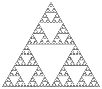
Figure 1: The fractal structure known as Sierpinski’s gasket has the overall shape of an equilateral triangle, subdivided recursively into smaller equilateral triangles. It is self-similar at all length scales, so no matter how much one enlarges a small area of the gasket, one encounters the same pattern of recursively nested triangles.

Let us first see how the dimension of a system influences its resistance. Fig. 2 shows a standard set-up; a rectangular block of a material with resistivity $\rho$, that has length $L$ and cross-sectional area $A$, admits a current of $I$ when a potential difference is applied across its length. The resistance of this block is simply given by $R=\rho L/A$. Now let us consider making the cross-section very small $A=d^{2}$ where $d\ll L$. This produces an effectively one-dimensional conductor, and clearly its resistance will scale linearly with its length, $R\propto L$. Now let us change one of the transverse dimensions to $L$, giving a cross-sectional area of $A=Ld$, so that the sample forms a thin sheet. In this case we obtain the somewhat counter-intuitive result that $R$ is constant, that is, the resistance of a two-dimensional conductor does not depend on its area. Finally, if we consider a cube by setting $A=L^{2}$, it is clear that $R\propto 1/L$. If we write the scaling of the resistance as $R\propto L^{\eta}$, we can combine these results to show that the Euclidean dimension of the system, $D_{E}$, is related to the scaling of the resistance by the relation:

$$\eta=2-D_{E}\ .$$ (1)

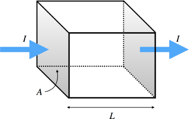
Figure 2: Geometry to define the resistance of a block of material with resistivity $\rho$. A current $I$ enters and leaves through the shaded faces which have each a cross-sectional area of $A$. If the length of the block is $L$, its resistance is $R=\rho L/A$.

Fractional dimension – Looking at Fig. 1, the Sierpinski gasket intuitively has a dimension that is smaller than that of a standard two-dimensional triangle, but is larger than a line. How can we define such a fractional dimension? The key is to study how the size, or “hypervolume”, of an object increases as it is enlarged. For an object with integer dimension $D$, doubling its side-length increases its hypervolume by a factor of $2^{D}$. For example, doubling the side-length of a square produces a new square that is 4 times larger than the original indicating that (as expected) $D=2$, while doubling the side-length of a cube increases its volume by a factor of 8, meaning than $D=3$. This permits an alternative definition of dimension, the Hausdorff dimension, which agrees with $D_{E}$ for integer dimensions, but can also be applied to fractal objects. From Fig. 3 it is clear that doubling the length of the triangle sides produces three copies of the Sierpinski gasket; for example the $n=3$ level network has twice the side-length of the $n=2$ network, and contains three copies of it. Solving the relation $3=2^{D}$ reveals that the Hausdorff dimension of the Sierpinski gasket is $D=\log_{2}3\simeq 1.585$. As anticipated, this value lies between 1 and 2.

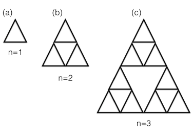
Figure 3: The fractal Sierpinski gasket shown in Fig.1 can be obtained as the $n\rightarrow\infty$ limit of recursively dividing a triangle. Here we show the (a) $n=1$, (b) $n=2$, and (c) $n=3$ levels of this process. Compare with the resistor networks shown in Fig. 5 which provide a physical implementation of these structures.

Resistance scaling – It is tempting to obtain the scaling of the resistance of Sierpinski’s gasket, measured between two of its exterior corners, by directly substituting this value for $D$ in Eq. 1. The fractal nature of the system, however, means that we must calculate its resistance with more care. Fig. 3 shows how the gasket can be produced by a recursive process. Level 1 (Fig. 3a) consists of a single upward-pointing triangle. To reach level 2 (Fig. 3b) this triangle is enlarged by a factor of two, and then subdivided to form three upward-pointing triangles. The same procedure – scaling every upward-pointing triangle by two and then subdividing into three – is then applied to create the level 3 network (Fig. 3c). Continuing this process indefinitely produces the true Sierpinski gasket shown in Fig. 1.

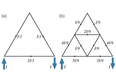
Figure 4: Current flowing through the (a) level-1 and (b) level-2 approximations to Sierpinski’s gasket. Kirchoff’s laws are used to find the currents flowing through each resistance.

The resistance of the level-1 configuration can be obtained easily by expressing it in terms of series and parallel resistances. Higher levels are more challenging to treat in this way, but can be analyzed (see Ref. Ching et al. (1994)) using the “star-triangle” method (also sometimes called $\Delta-Y$ method), or applying nodal analysis Allen and Liu (2015). However, an alternative approach is to use Kirchoff’s laws. The level-2 system shown in Fig. 4b is sufficiently simple that the internal currents can be obtained by the students (with some prompting) through trial and error, noting that the currents entering a node must equal the currents exiting it, and that the sum of the currents around a closed loop must be equal to zero. Alternatively it is straightforward to write the simultaneous equations satisfied by the currents, and solve the problem algebraically. We can see directly that the majority of the current flows along the bottom edge, indicating that the current flow is predominantly one-dimensional, with the incursions into the bulk of the system producing small modifications from this behaviour. Let us suppose that each side of every triangle has a resistance of $R_{0}$. From the configurations of current shown in Fig. 4 it can be seen that the net resistance between the two corners of the level-1 system is given by $2R_{0}/3$, while the level-2 resistance is $10R_{0}/9$, the two differing by a factor of $5/3$. That is to say, for the purposes of measuring resistance by connecting external probes, the level-2 network composed of resistors of value $R$ can be replaced by a level-1 network with resistors of $5R/3$.

This process can be repeated to analyze ever-higher fractal levels. A level-3 network (see Fig. 3c) can first be reduced to a level-2 network by scaling the resistances by a factor of $5/3$, which, as seen above, can then be reduced in turn to an level-1 network, introducing another factor of $5/3$. The resistance of a level-$n$ network is thus given by the power-law

$$R_{n}=\frac{2R_{0}}{3}\ \left(\frac{5}{3}\right)^{n-1}\ .$$ (2)

This form of analysis, finding a scaling law for the value of a quantity as fine structure is successively eliminated, is very similar to the real-space renormalization group transformations used to analyze second-order phase transitions Maris and Kadanoff (1978).

From this scaling analysis we now know the corner-corner resistance of a level-$n$ approximation to Sierpinski’s gasket. It is also clear (see Fig. 3) that the side-length of a level-$n$ network is given by $L=2^{n-1}$. This relationship can be used to eliminate $\left(n-1\right)$ from Eq. 2, in order to obtain the dependence of the resistance on $L$. Some straightforward algebra yields the result

$$R(L)=\frac{2R_{0}}{3}\ L^{\log_{2}\left(5/3\right)}\simeq\frac{2R_{0}}{3}\ L^{0.737}\ .$$ (3)

If, as before, we write the scaling of the resistance as $R\propto L^{\eta}$, we can thus obtain the exponent, $\eta$, as:

$$\eta= = \log_{2}\left(\frac{5}{3}\right)$$ (4)

$$= \log_{2}5-D$$

where $D=\log_{2}3$ is the Hausdorff dimension of the Sierpinski gasket. This equation is the fractional dimension analogue to Eq. 1.

Implementation – To provide a physical realization of the networks shown in Fig. 3, the basic triangular building block was obtained by soldering three 1 k$\Omega$ metal film resistors (0.5W, tolerance 1%) in a triangle as shown in Fig. 5a. These blocks could then be connected with jumper links, cheap and easily available components used in microelectronics, to construct the various resistor networks. The corner-corner resistance can be easily measured using an ohmmeter, or alternatively by connecting the network across a bench power supply and measuring the input current and voltage dropped across it. Having connected three triangular elements to create the level-2 network, students can then build and connect further copies to create the level-3 network, and so on. The largest network used in practice was of level 5 (Fig. 6), for which three groups of students can contribute their level-4 networks. In principle even higher orders can be obtained, if sufficient triangular elements are prepared.

To observe the fractional scaling of the resistance, we measure the corner-corner resistance for the different fractal levels. From Eq. 3 it is clear that

$$\log R=\eta\log L+\log\left(2R_{0}/3\right)\ ,$$ (5)

where $\eta=\log_{2}\left(5/3\right)$, and so making a log-log plot of this data will yield a straight line with a slope of $\eta$. Fig. 7 shows some typical data obtained in this experiment. Error bars were estimated from the statistical variance of the three resistances measured between the pairs of exterior corners of each network. Making a linear regression to these data points yields a value of $\eta=0.743\pm 0.002$, in excellent agreement with the theoretical value of $\eta=0.737$. Students found it particularly gratifying to obtain results of such high precision, using such a “low-tech” construction method.

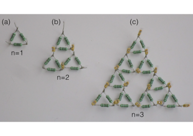
Figure 5: (a) The basic element of the resistor network, three 1 k$\Omega$ resistors connected in a triangle. (b) Level-2 of the Sierpinski gasket, obtained by connecting three triangular elements with jumper links. (c) Level-3 of the Sierpinski gasket.

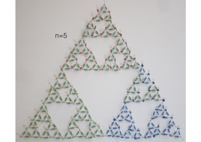
Figure 6: The highest level ($n=5$) network considered in this work, containing 81 triangular elements and 243 individual resistors.

The students clearly enjoyed the process of building the resistor networks, and the process allowed them to become more engaged with the apparatus than normal. In electricity and magnetism practicals, the majority of the components are provided essentially as “black boxes” to be plugged into circuit boards in highly specific arrangements, and so the construction process proved to be a stimulating change. In particular students exhibited considerable pride in successfully completing the largest (level-5) network which has a rather striking, and notably fractal, appearance when laid out on the bench.

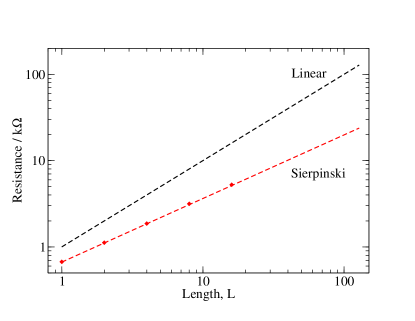
Figure 7: Power-law scaling of the corner-corner resistance in a Sierpinski resistance network. The error bars on the data points are smaller than the symbol size. The resistance follows a power-law dependence on the side-length of the network, following the theoretical result (Eq. 5, shown by the dashed red line) to an excellent degree of accuracy. For comparison, the linear scaling of a one-dimensional array of resistors is shown by the black dashed line.