Generalized Gibbs ensemble of the Ablowitz-Ladik lattice, Circular $\beta$-ensemble and double confluent Heun equation

Abstract

We consider the discrete defocusing nonlinear Schrödinger equation in its integrable version, which is called defocusing Ablowitz-Ladik lattice. We consider periodic boundary conditions with period $N$ and initial data sample according to the Generalized Gibbs ensemble. In this setting, the Lax matrix of the Ablowitz-Ladik lattice is a random CMV-periodic matrix and it is related to the Killip-Nenciu Circular $\beta$-ensemble at high-temperature. We obtain the generalized free energy of the Ablowitz-Ladik lattice and the density of states of the random Lax matrix by establishing a mapping to the one-dimensional log-gas. For the Gibbs measure related to the Hamiltonian of the Ablowitz-Ladik flow, we obtain the density of states via a particular solution of the double-confluent Heun equation.

1 Introduction

The defocusing Ablowitz–Ladik (AL) lattice for the complex functions $\alpha_{j}(t)$, $j\in{\mathbb{Z}}$ and $t\in{\mathbb{R}}$, is the system of nonlinear equations

$$i\dot{\alpha}_{j}=-(\alpha_{j+1}+\alpha_{j-1}-2\alpha_{j})+|\alpha_{j}|^{2}(\alpha_{j-1}+\alpha_{j+1})\,,$$ (1.1)

where $\dot{\alpha}_{j}=\dfrac{d\alpha_{j}}{dt}$. We assume $N$-periodic boundary conditions $\alpha_{j+N}=\alpha_{j}$, for all $j\in{\mathbb{Z}}$. The AL lattice was introduced by Ablowitz and Ladik [1, 2] as the spatial integrable discretization of the defocusing cubic nonlinear Schrödinger Equation (NLS) for the complex function $\psi(x,t)$, $x\in S^{1}$ and $t\in{\mathbb{R}}$:

$$i\partial_{t}\psi(x,t)=-\partial^{2}_{x}\psi(x,t)+2\lvert\psi(x,t)\rvert^{2}\psi(x,t).$$ (1.2)

The cubic NLS equation was proved to be integrable by Zakharov and Shabat [70].

It is straightforward to verify that the quantity

$$K^{(0)}:=\prod_{j=1}^{N}\left(1-|\alpha_{j}|^{2}\right)\,,$$ (1.3)

is a constant of motion for the AL lattice, namely $\dfrac{d}{dt}K^{(0)}=0$. This implies that if $|\alpha_{j}(0)|<1$ for all $j\in{\mathbb{Z}}$, then $|\alpha_{j}(t)|<1$ for all $t>0$. We chose the $N$-dimensional disc ${\mathbb{D}}^{N}$ as the phase space of the AL lattice, here ${\mathbb{D}}=\{z\in{\mathbb{C}}\,|\,|z|<1\}$. On ${\mathbb{D}}^{N}$ we introduce the symplectic form [23, 30]

$$\omega=i\sum_{j=1}^{N}\frac{1}{\rho_{j}^{2}}{\rm d}\alpha_{j}\wedge{\rm d}{\overline{\alpha}}_{j}\,,\quad\rho_{j}=\sqrt{1-|\alpha_{j}|^{2}}.$$ (1.4)

The corresponding Poisson bracket is defined for functions $f,g\in{\mathcal{C}}^{\infty}({\mathbb{D}}^{N})$ as

$$\begin{split}\{f,g\}&=i\sum_{j=1}^{N}\rho_{j}^{2}\left(\frac{\partial f}{\partial{\overline{\alpha}}_{j}}\frac{\partial g}{\partial\alpha_{j}}-\frac{\partial f}{\partial\alpha_{j}}\frac{\partial g}{\partial{\overline{\alpha}}_{j}}\right)\,.\end{split}$$ (1.5)

The phase shift $\alpha_{j}(t)\to e^{-2it}\alpha_{j}(t)$ transforms the AL lattice into the equation

$$i\dot{\alpha}_{j}=-\rho_{j}^{2}(\alpha_{j+1}+\alpha_{j-1}),\quad\rho_{j}=\sqrt{1-|\alpha_{j}|^{2}},$$ (1.6)

which we call the reduced AL equation. We remark that the quantity $-2\ln(K^{(0)})$ is the generator of the shift $\alpha_{j}(t)\to e^{-2it}\alpha_{j}(t)$, while $H_{1}=K^{(1)}+{\overline{K^{(1)}}}$ with

$$K^{(1)}:=-\sum_{j=1}^{N}\alpha_{j}\overline{\alpha}_{j+1},$$ (1.7)

generates the flow (1.6). The AL equations (1.1) have the Hamiltonian structure

$$\dot{\alpha}_{j}=\{{\alpha}_{j},H_{AL}\},\quad H_{AL}(\alpha_{j},\overline{{\alpha}}_{j})=-2\ln(K^{(0)})+K^{(1)}+\overline{K^{(1)}}.$$ (1.8)

Integrability.

As we have already said, the AL lattice was discovered by Ablowitz and Ladik by discretizing the $2\times 2$ Zakharov-Shabat Lax pair [1] of the cubic nonlinear Schrödinger equation. For a comprehensive review see [3]. The integrability of the Ablowitz–Ladik system has also been proved by constructing a bi-Hamiltonian structure [23, 9]. A techniques to calculate the $\tau$-function correlators has been introduced in [15].

Using the connection between orthogonal polynomials on the unit circle and the AL lattice, Nenciu and Simon [54, 59] constructed a new Lax pair for the AL lattice that sometimes is referred to as the big Lax pair and which put the AL equation on the same foot as the Toda lattice. The link between orthogonal and biorthogonal polynomials on the unit circle and the Ablowitz–Ladik hierarchy (see also [4], [43]) is the analogue of the celebrated link between the Toda hierarchy and orthogonal polynomials on the real line (see e.g. [19]). This link was also generalized to the non-commutative case [14] (see also [16]). Generalization of this construction to other integrable equations has been considered in [55].

To construct the big Lax pair, we follow [54, 59] and we double the size of the chain according to the periodic boundary conditions, thus we consider a chain of $2N$ particles $\alpha_{1},\ldots,\alpha_{2N}$ such that $\alpha_{j}=\alpha_{j+N}$ for $j=1,\ldots,N$. Define the $2\times 2$ unitary matrix $\Xi_{j}$

$$\Xi_{j}=\begin{pmatrix}{\overline{\alpha}}_{j}&\rho_{j}\\ \rho_{j}&-\alpha_{j}\end{pmatrix}\,,\quad j=1,\dots,2N\,,$$ (1.9)

and the $2N\times 2N$ matrices

$${\mathcal{M}}=\begin{pmatrix}-\alpha_{2N}&&&&&\rho_{2N}\\ &\Xi_{2}\\ &&\Xi_{4}\\ &&&\ddots\\ &&&&\Xi_{2N-2}\\ \rho_{2N}&&&&&{\overline{\alpha}}_{2N}\end{pmatrix}\,,\qquad{\mathcal{L}}=\begin{pmatrix}\Xi_{1}\\ &\Xi_{3}\\ &&\ddots\\ &&&\Xi_{2N-1}\end{pmatrix}\,.$$ (1.10)

Now let us define the unitary Lax matrix

$${\mathcal{E}}={\mathcal{L}}{\mathcal{M}}\,,$$ (1.11)

that has the structure of a $5$-band diagonal matrix

$$\begin{pmatrix}*&*&*&&&&&&&*\\ *&*&*&&&&&&&*\\ &*&*&*&*&&&&&\\ &*&*&*&*&&&&&\\ &&&&&\ddots&\ddots&&&\\ &&&&&&*&*&*&*\\ &&&&&&*&*&*&*\\ *&&&&&&&*&*&*\\ *&&&&&&&*&*&*\\ \end{pmatrix}\,.$$

The matrix ${\mathcal{E}}$ is a periodic CMV matrix (after Cantero Morales and Velsquez [17]). The $N$-periodic reduced AL equation (1.6) is equivalent to the following Lax equation for the matrix ${\mathcal{E}}$:

$$\dot{\mathcal{E}}=i\left[{\mathcal{E}},{\mathcal{E}}^{+}+({\mathcal{E}}^{+})^{\dagger}\right]\,,$$ (1.12)

where ^† stands for hermitian conjugate and

$${\mathcal{E}}^{+}_{j,k}=\begin{cases}\frac{1}{2}{\mathcal{E}}_{j,j}\quad j=k\\ {\mathcal{E}}_{j,k}\quad k=j+1\,{\,{\rm mod}\,}\,2N\,\mbox{or}\,k=j+2\,{\,{\rm mod}\,}\,2N\\ 0\quad\mbox{otherwise}.\end{cases}$$ (1.13)

We observe that $({\mathcal{E}}^{+})^{\dagger}+({\mathcal{E}}^{\dagger})^{+}={\mathcal{E}}^{\dagger}$ and $[{\mathcal{E}},{\mathcal{E}}^{\dagger}]=0$ because ${\mathcal{E}}$ is unitary. Therefore, one can write the equation (1.12) in the equivalent form

$$\dot{\mathcal{E}}=i\left[{\mathcal{E}},{\mathcal{E}}^{+}-({\mathcal{E}}^{\dagger})^{+}\right]\,.$$ (1.14)

The formulation (1.12) implies that the quantities

$$K^{(\ell)}=\frac{\mbox{Tr}\left({\mathcal{E}}^{\ell}\right)}{2},\quad\ell=1,\dots,N-1,$$ (1.15)

are constants of motion for the defocusing AL system. For example

$$K^{(1)}=-\sum_{j=1}^{N}\alpha_{j}\overline{\alpha}_{j+1},\quad K^{(2)}=\sum_{j=1}^{N}[(\alpha_{j}\overline{\alpha}_{j+1})^{2}-2\alpha_{j}\overline{\alpha}_{j+2}\rho_{j+1}^{2}]\,.$$

Furthermore, $K^{(0)},K^{(1)},\dots,K^{(N-1)}$ are functionally independent and in involution, showing that the $N$-periodic AL system is integrable [54, 1, 3].

Remark 1.1.

The quantity $2\Re(K^{(1)})$ generates the reduces AL equation (1.6), while the quantity $-2\Im(K^{(1)})$ generates the flow

$$\dot{\alpha}_{j}=(1-|\alpha_{j}|^{2})(\alpha_{j+1}-\alpha_{j}),$$

which is called Schur flow. The Schur flow emerges in [2] as a spatial discretization of the defocusing modified Korteweg–de Vries equation

$$\partial_{t}f-6f\partial_{x}f+\partial_{x}^{3}f=0.$$

For the integration of the Schur flow and its relation to orthogonal polynomial on the unit circle see [32, 60].

Generalized Gibbs Ensemble for the Ablowitz–Ladik Lattice.

The symplectic form $\omega$ in (1.4) induces on ${\mathbb{D}}^{N}$ the volume form ${\rm d}\mbox{vol}=\dfrac{1}{K^{(0)}}{\rm d}^{2}{\boldsymbol{\alpha}}$, with ${\rm d}^{2}{\boldsymbol{\alpha}}=\prod_{j=1}^{N}(i{\rm d}\alpha_{j}\wedge{\rm d}{\overline{\alpha}}_{j}\,)$. We observe that $\int_{\overline{{\mathbb{D}}}^{N}}{\rm d}\mbox{vol}=\infty$, however, we can define the Gibbs measure with respect to the Hamiltonian $H_{AL}$ in (1.8):

$$\frac{1}{Z_{\beta}}e^{-\frac{\beta}{2}H_{AL}}{\rm d}\mbox{vol}=\frac{1}{Z_{\beta}}e^{\beta\Re(K^{(1)})}\prod_{j=1}^{N}(1-|\alpha_{j}|^{2})^{\beta-1}{\rm d}^{2}{\boldsymbol{\alpha}},\quad\beta>0,$$ (1.16)

where $Z_{\beta}=\int_{\overline{{\mathbb{D}}}^{N}}e^{\beta\Re(K^{(1)})}\prod_{j=1}^{N}(1-|\alpha_{j}|^{2})^{\beta-1}{\rm d}^{2}{\boldsymbol{\alpha}}<\infty$ is the normalizing constant. The above probability measure is clearly invariant under the Hamiltonian flow ${\alpha}_{j}(0)\to{\alpha}_{j}(t)$ associated to the Ablowitz–Ladik equation (1.1).

Since the Ablowitz–Ladik lattice posses several conserved quantities (1.15), one can introduce a Generalized Gibbs Ensemble on the phase space ${\mathbb{D}}^{N}$ in the following way. Fix ${\mathbb{N}}\ni\kappa\leq N-1$ and let us define

$$V(z)=\sum_{m=1}^{\kappa}\eta_{m}\Re(z^{m})\,,$$ (1.17)

where $\eta_{m}\in{\mathbb{R}}$ are called chemical potentials. Then

$$\mbox{Tr}\left(V\left({\mathcal{E}}\right)\right)=\sum_{m=1}^{\kappa}\eta_{m}(K^{(m)}+\overline{K^{(m)}}),$$

where $K^{(m)}$ are the AL conserved quantities (1.15). The finite volume Generalized Gibbs measure can be written as:

$${\rm d}\mathbb{P}_{AL}({\alpha}_{1},\ldots,{\alpha}_{N})=\frac{1}{Z^{AL}_{N}(V,\beta)}\prod_{j=1}^{N}\left(1-|\alpha_{j}|^{2}\right)^{\beta-1}\exp\left(-\mbox{Tr}\left(V\left({\mathcal{E}}\right)\right)\right){\rm d}^{2}{\boldsymbol{\alpha}}\,,$$ (1.18)

where $Z^{AL}_{N}(V,\beta)$ is the partition function of the system:

$$Z^{AL}_{N}(V,\beta)=\int_{{\mathbb{D}}^{N}}\prod_{j=1}^{N}\left(1-|\alpha_{j}|^{2}\right)^{\beta-1}\exp\left(-\mbox{Tr}\left(V\left({\mathcal{E}}\right)\right)\right){\rm d}^{2}{\boldsymbol{\alpha}}\,.$$ (1.19)

Choosing the initial data of the Ablowitz–Ladik lattice according to the Generalized Gibbs measure (1.18), the Lax matrix ${\mathcal{E}}$ turns into a random matrix. In [51] Mendl and Sphon study the dynamic of the Ablowitz–Ladik lattice at non-zero temperature. They study numerically correlation functions and in particular, introducing the density $\delta_{j}=\Re(\alpha_{j+1}\overline{\alpha}_{j})$, they study the density-density correlation function

$${\bf E}\left[\delta_{j}(t)\delta_{1}(0)\right]-{\bf E}\left[\delta_{j}(t)\right]{\bf E}\left[\delta_{1}(0)\right]\,,$$

where ${\bf E}\left[\cdot\right]$ is the expectation with respect to Gibbs measure (1.16). They showed numerically that density-density time correlations in thermal equilibrium have symmetrically located peaks, which travel in opposite directions at constant speed, broaden ballistically and decay as $1/t^{\gamma}$ when $t\to\infty$, where the scaling exponent $\gamma$ is approximately equal to one. This behaviour is believed to be typical of integrable nonlinear systems.

More quantitative results have been obtained for linear (integrable) systems and for the Toda lattice. It was shown in [34] that the fastest peaks of the correlation functions of harmonic oscillators with short range interactions have a Airy type scaling. Regarding nonlinear integrable systems in [61] Spohn was able to connect the Gibbs ensemble of the Toda lattice to the Dumitriu-Edelman $\beta$-ensemble [21]. In this way, the generalized Gibbs free energy of the Toda chain turns out to be related to the $\beta$-ensembles of random matrix theory in the mean-field regime [22, 7]. The behaviour of the correlation functions of the Toda chains has been derived by applying the theory of generalized hydrodynamic [62, 20]. We mention also the recent work [36], where the authors derive a large deviation principle for the mean density of states for the Generalized Gibbs measure of the Toda lattice.

2 Statement of the results

In this manuscript we derive the mean density of states $\mu^{\beta}_{AL}$ of the random Lax matrix $\mathcal{E}$ sampled according to generalized Gibbs measure (1.18) and we determine the free energy of the AL generalized Gibbs ensemble

$$F_{AL}(V,\beta)=\lim_{N\to\infty}\frac{1}{N}\log Z^{AL}_{N}(V,\beta).$$

This is achieved by connecting the generalized Gibbs ensemble of the Ablowitz–Ladik lattice to the Killip-Nenciu [42] matrix Circular $\beta$-ensemble at high-temperature investigated by Hardy and Lambert [37]. Further connections between discrete integrable systems with Gibbs measure initial data and classes of random matrices has been explored in [33]. For connections between integrable PDEs and random objects see [6].

Let $\mathcal{M}(\mathbb{T})$ be the space of probability measures on the torus $\mathbb{T}=[-\pi,\pi]$ and for $\mu\in\mathcal{M}(\mathbb{T})$ let us consider the functional

$$\begin{split}{\mathcal{F}}^{(V,\beta)}(\mu)&=2\int\limits_{\mathbb{T}}V(\theta)\mu(\theta){\rm d}\theta-\beta\int\int\limits_{\hskip-5.69046pt\mathbb{T}\times\mathbb{T}}\ln\sin\left(\frac{|\theta-\phi|}{2}\right)\mu(\theta)\mu(\phi){\rm d}\theta{\rm d}\phi\\ &+\int\limits_{\mathbb{T}}\ln\left(\mu(\theta)\right)\mu(\theta){\rm d}\theta+\ln(2\pi)\,.\end{split}$$ (2.1)

Remark 2.1.

Here and below, we make an abuse of notation by denoting the potential $V(z)=V(e^{i\theta})$ simply by $V(\theta)$.

For sufficiently regular potential $V(\theta)$, the functional (2.1) has a unique minimizer $\mu_{HT}^{\beta}({\rm d}\theta)=\mu_{HT}^{\beta}(\theta){\rm d}\theta$, [58], that describes the density of states of the Circular $\beta$-ensemble at high-temperature [37]. For finite $\beta$ and smooth potentials $V(\theta)$, it has been shown by Hardy and Lambert in [37] that the minimizer $\mu_{HT}^{\beta}({\rm d}\theta)$ has a smooth density and its support is the whole torus $\mathbb{T}$.

Theorem 2.2 (First Main theorem).

Consider $\beta>0$ and a smooth potential $V$ as in (1.17) on the unit circle $\mathbb{T}$. The mean density of states $\mu_{AL}^{\beta}({\rm d}\theta):=\mu_{AL}^{\beta}(\theta){\rm d}\theta$ of the Ablowitz–Ladik Lax matrix ${\mathcal{E}}$ in (1.11) endowed with the probability (1.18) is absolutely continuous with respect to the Lebesgue measure and takes the form

$$\mu_{AL}^{\beta}(\theta)=\partial_{\beta}\left(\beta\mu_{HT}^{\beta}(\theta)\right)\;a.e.,$$ (2.2)

where $\mu_{HT}^{\beta}$ is the unique minimizer of the functional (2.1).

To prove the above theorem we derive a relation (see Proposition 4.2) between the free energy of the $\beta$-ensembles at high-temperature, namely the minimum value of the minimizer (2.1)

$$F_{HT}(V,\beta):={\mathcal{F}}^{(V,\beta)}(\mu^{\beta}_{HT}),$$

and the free energy $F_{AL}(V,\beta)$ of the AL lattice:

$$F_{AL}(V,\beta)=\partial_{\beta}\left(\beta F_{HT}(V,\beta)\right)+\ln(2).$$

Such relation is obtained via transfer operator techniques.

The particular case $V(\theta)=2\eta\cos\theta$ corresponds to the free energy associated to the AL equation (1.1), and we show that the minimizer of the functional (2.1) is obtained via a particular solution of the Double Confluent Heun (DCH) equation.

Theorem 2.3 (Second main theorem).

Fix $\beta>0$ and let $V(\theta)=\eta\cos\theta$, where $\eta$ is a real parameter. There exists $\varepsilon>0$ such that for all $\eta\in(-\varepsilon,\varepsilon)$, the minimizer $\mu_{HT}^{\beta}({\rm d}\theta)=\mu^{\beta}_{HT}(\theta){\rm d}\theta$ of the functional (2.1) takes the form

$$\mu^{\beta}_{HT}(\theta)=\frac{1}{2\pi}+\frac{1}{\pi\beta}\Re\left(\frac{zv^{\prime}(z)}{v(z)}\right)_{\big{|}z=e^{i\theta}}\,,$$ (2.3)

where $v(z)$ is the unique solution (up to a multiplicative non-zero constant) of the Double Confluent Heun (DCH) equation

$$z^{2}v^{\prime\prime}(z)+\left(-\eta+z(\beta+1)+\eta z^{2}\right)v^{\prime}(z)+\eta\beta(z+\lambda)v(z)=0\,$$ (2.4)

analytic for $|z|\leq r$ with $r\geq 1$. Such solution is differentiable in the parameter $\eta$ and $\beta$. The parameter $\lambda=\lambda(\eta,\beta)$ in (2.4) is determined for $\eta\in(-\varepsilon,\varepsilon)$ by the solution of the equation

$$\lambda(R_{1})_{11}+\frac{\eta}{\beta+1}(R_{1})_{21}=0,\quad$$ (2.5)

with the condition $\lambda(\eta=0,\beta)=0$. In the above expression $(R_{1})_{jk}$ is the $jk$ entry of the matrix $R_{1}$ which is defined by the infinite product

$$R_{1}=M_{1}M_{2}\dots M_{k}\dots,\quad M_{k}=\begin{pmatrix}1+\frac{\lambda\beta\eta}{k(k+\beta)}&\frac{\eta^{2}}{k(k+\beta+1)}\\ 1&0\end{pmatrix}\,.$$

We remark that the solution of the double confluent Heun equation has generically an essential singularity at $z=0$ and $z=\infty$, and one needs to tune the accessory parameter $\lambda$ to obtain an analytic solution, for a review see [57]. In our derivation of (2.4) the parameter $\lambda$ coincides with the first moment of the measure $\mu(\theta)$, namely $\lambda=\int_{\mathbb{T}}\mu(\theta)e^{i\theta}d\theta$. It is a transcendental function of $\beta$ and $\eta$ and it is related to the Painlevé III equation [24, 47].

Remark 2.4.

Under the change of variable

$$v(z)=\exp\left(-\frac{\eta}{2}\left(z+\frac{1}{z}\right)\right)z^{-\frac{\beta+1}{2}}f(z)\,,$$

the DCH equation (2.4) takes the form of a Schrödinger equation

$$f^{\prime\prime}(z)+q(z)f(z)=0,$$

with potential $q(z)$ singular at the origin

$$q(z)=\frac{1}{z^{2}}\left(\eta\frac{\beta-1}{2}\left(z+\frac{1}{z}\right)-\frac{\eta^{2}}{4}\frac{(z^{2}-1)^{2}}{z^{2}}-\frac{1}{4}(\beta^{2}+4\beta+3)+\eta\beta\lambda\right).$$

Remark 2.5.

For the case $V=0$ it was shown in [37] that the minimizer of the functional (3.18) is the uniform measure on the circle, while for the case $V(\theta)=\beta V(\theta)$ and $\beta\to\infty$ the minimizer of (2.1) was considered in [49]. The particular case $V(\theta)\to\beta\eta\cos\theta$ and $\beta\to\infty$ has first been considered by Gross–Witten [35] and Baik–Deift–Johansson [11]. The measure (2.3) in Theorem 2.3 generalizes the result of Gross and Witten [35] and Baik–Deift–Johansson [11] to the high-temperature regime (see Remark 5.6).

This manuscript is organized as follows. In section 3 we introduce the Circular $\beta$ ensemble and its high-temperature limit. Then we review results in the literature on Circular $\beta$ ensemble and we derive some technical results needed to prove our main theorems. In section 4 we prove our first main theorem, namely Theorem 2.2 and in section 5 we prove Theorem 2.3. Finally, the most technical parts of our arguments are deferred to the appendices.

3 Circular $\beta$ Ensemble at high-temperature

The Circular Ensemble at temperature $\tilde{\beta}^{-1}$ is a system of $N$ identical particles on the one-dimensional torus $\mathbb{T}=[-\pi,\pi]$ with distribution

$${\rm d}\mathbb{P}_{\tilde{\beta}}(\theta_{1},\ldots,\theta_{N})=\frac{1}{Z^{C\tilde{\beta}E}_{N}}\prod_{j<\ell}|e^{i\theta_{\ell}}-e^{i\theta_{j}}|^{{\widetilde{\beta}}}{\rm d}\boldsymbol{\theta},\quad{\rm d}\boldsymbol{\theta}={\rm d}\theta_{1}\dots\rm d\theta_{N}\,,$$ (3.1)

where $Z_{N}^{C\tilde{\beta}E}>0$ is the norming constant, or partition function of the system. For $\tilde{\beta}=1,2,4$ Dyson observed that the above measure corresponds to the eigenvalue distribution of circular orthogonal ensemble (COE), circular unitary ensemble (CUE) and circular symplectic ensemble (CSE) of random matrix ensembles (see e.g. [50, 25]). For general $\tilde{\beta}>0$, Killip and Nenciu proved that the Circular $\beta$ Ensemble can be associated to the eigenvalue distribution of a random sparse matrix, the so-called CMV matrix, after Cantero, Moral, Velázquez [17]. To state their result, we need the following definition.

Definition 3.1.

A complex random variable $X$ with values on the unit disk ${\mathbb{D}}$ is $\Theta_{\nu}$-distributed ($\nu>1$) if

$${\bf E}\left[f(X)\right]=\frac{\nu-1}{2\pi}\int_{\overline{{\mathbb{D}}}}f(z)(1-|z|^{2})^{\frac{\nu-3}{2}}{\rm d}^{2}z\,.$$ (3.2)

for any measurable function $f\,:\,{\mathbb{D}}\to{\mathbb{C}}$. When $\nu=1$, $\Theta_{1}$ is the uniform distribution on the unit circle $S^{1}$.

We recall that for ${\mathbb{N}}\ni\nu\geq 2$, such measure has the following geometrical interpretation: if $\mathbf{u}=(u_{1},u_{2},\dots,u_{\nu+1})$ is chosen at random according to the surface measure on the unit sphere $S^{\nu}$ in $\mathbb{R}^{\nu+1}$, then $u_{1}+iu_{2}$ is $\Theta_{\nu}-$distributed. We can now state the result of Killip-Nenciu.

Theorem 3.2 (cf. [42] Theorem 1).

Consider the block diagonal $N\times N$ matrices

$$M=\mbox{diag}\left(\Xi_{1},\Xi_{3},\Xi_{5}\ldots,\right)\quad\mbox{ and }\quad L=\mbox{diag}\left(\Xi_{0},\Xi_{2},\Xi_{4},\ldots\right)\,,$$ (3.3)

where the block $\Xi_{j}$, $j=1,\dots,N-1$, takes the form

$$\Xi_{j}=\begin{pmatrix}{\overline{\alpha}}_{j}&\rho_{j}\\ \rho_{j}&-\alpha_{j}\end{pmatrix}\,,\;\;\rho_{j}=\sqrt{1-|\alpha_{j}|^{2}},$$ (3.4)

while $\Xi_{0}=(1)$ and $\Xi_{N}=({\overline{\alpha}}_{N})$ are $1\times 1$ matrices. Define the $N\times N$ sparse matrix

$$E=LM,$$ (3.5)

and suppose that the entries $\alpha_{j}$ are independent complex random variables with $\alpha_{j}\sim\Theta_{{\widetilde{\beta}}(N-j)+1}$ for $1\leq j\leq N-1$ and $\alpha_{N}$ is uniformly distributed on the unit circle. Then the eigenvalues of $E$ are distributed according to the Circular Ensemble (3.1) at temperature $\tilde{\beta}^{-1}$.

We observe that each of the matrices $\Xi_{j}$ is unitary, and so are the matrices $L$ and $M$. As a result, the eigenvalues of $E$ clearly lie on the unit circle. The matrix $E$ is a $5$-diagonal unitary matrix that takes the form

$$E=\begin{pmatrix}\bar{\alpha}_{1}&\rho_{1}\bar{\alpha}_{2}&\rho_{1}\rho_{2}&&&&&&\\ \rho_{1}&-\alpha_{1}\bar{\alpha}_{2}&-\alpha_{1}\rho_{2}&&&&&&\\ &\rho_{2}\bar{\alpha}_{3}&-\alpha_{2}\bar{\alpha}_{3}&\rho_{3}\bar{\alpha}_{4}&\rho_{3}\rho_{4}&&&&\\ &\rho_{2}\rho_{3}&-\alpha_{2}\rho_{3}&-\alpha_{3}\bar{\alpha}_{4}&-\alpha_{3}\rho_{4}&&&&\\ &&&\ddots&\ddots&\ddots&\ddots&&&\\ &&&&&\rho_{N-3}\bar{\alpha}_{N-2}&-\alpha_{N-3}\bar{\alpha}_{N-2}&\rho_{N-2}\bar{\alpha}_{N-1}&\rho_{N-2}\rho_{N-1}\\ &&&&&\rho_{N-3}\rho_{N-2}&-\alpha_{N-3}\rho_{N-2}&-\alpha_{N-2}\bar{\alpha}_{N-1}&-\alpha_{N-2}\rho_{N-1}\\ &&&&&&&\bar{\alpha}_{N}\rho_{N-1}&-\alpha_{N-1}\bar{\alpha}_{N}\\ \end{pmatrix}\,.$$

We are interested in the probability distribution (3.1) when

• we add an external field, namely $d\theta_{i}\to e^{-2V(\theta_{i})}d\theta_{i}$ with $V:\mathbb{T}\to{\mathbb{R}}$ a smooth potential;

• we consider the limit ${\widetilde{\beta}}\to 0$ and $N\to\infty$ in such a way that ${\widetilde{\beta}}N=2\beta,\,\beta>0.$ Since ${\widetilde{\beta}}$ is interpreted as the inverse of the temperature, such limit is called high-temperature regime.

With the above changes, we arrive to the probability distribution of the Circular ensemble at high-temperature, and with an external potential:

$${\rm d}\mathbb{P}_{\beta}^{V}(\theta_{1},\ldots,\theta_{N})=\frac{1}{{\mathcal{Z}}^{HT}_{N}(V,\beta)}\prod_{j<\ell}|e^{i\theta_{\ell}}-e^{i\theta_{j}}|^{\frac{2\beta}{N}}e^{-2\sum_{j=1}^{N}V(\theta_{j})}{\rm d}\boldsymbol{\theta}\,,$$ (3.6)

where ${\mathcal{Z}}^{HT}_{N}(V,\beta)$ is the partition function of the system. Also in this case, we can associate to the above probability distribution a random CMV matrix. The lemma below has probably already appeared in the literature, but for completeness we provide the proof.

Lemma 3.3.

Let $E$ be the CMV matrix (3.5). Consider the block $2N\times 2N$ matrix

$${\widetilde{E}}=\mbox{diag}(E,E)\,,$$ (3.7)

whose entries are distributed according to

$${\rm d}\mathbb{P}({\alpha}_{1},\ldots,{\alpha}_{N})=\frac{1}{Z^{HT}_{N}(V,\beta)}\prod_{j=1}^{N-1}\left(1-|\alpha_{j}|^{2}\right)^{\beta\left(1-\frac{j}{N}\right)-1}e^{-\mbox{Tr}(V({\widetilde{E}}))}\prod_{j=1}^{N-1}{\rm d}^{2}\alpha_{j}\frac{{\rm d}\alpha_{N}}{i\alpha_{N}}\,.$$ (3.8)

Then the eigenvalues of ${\widetilde{E}}$ are all double, they lie on the unit circle and are distributed according to (3.6).

Moreover

$$Z^{HT}_{N}(V,\beta)=2^{1-N}\frac{\Gamma\left(\frac{\beta}{N}\right)^{N}}{\Gamma(\beta)}{\mathcal{Z}}^{HT}_{N}(V,\beta)\,,$$ (3.9)

where ${\mathcal{Z}}^{HT}_{N}(V,\beta)$ is the norming constant of the probability distribution (3.6) and $Z^{HT}_{N}(V,\beta)$ is the norming constant of the probability distribution (3.8).

Proof.

First, we notice that the eigenvalues of ${\widetilde{E}}$ are all double, since it is a block diagonal matrix with two identical blocks.

We consider the change of variables $\alpha_{N}\to e^{i\varphi}$, thus (3.8) becomes:

$${\rm d}\mathbb{P}({\alpha}_{1},\ldots,\alpha_{N-1},\varphi)=\frac{\prod_{j=1}^{N-1}\left(1-|\alpha_{j}|^{2}\right)^{\beta\left(1-\frac{j}{N}\right)-1}e^{-\mbox{Tr}(V({\widetilde{E}}))}\prod_{j=1}^{N-1}{\rm d}^{2}\alpha_{j}{\rm d}\varphi}{Z^{HT}_{N}(V,\beta)}\,.$$ (3.10)

Now, let $e^{i\theta_{1}},\ldots,e^{i\theta_{N}}$ be the eigenvalues of the CMV matrix $E$ endowed with probability (3.8), and let $q_{1},\ldots,q_{N}$ be the entries of the first row of the unitary matrix $Q$ such that $Q^{\dagger}\Theta Q=E$ where $\Theta=\mbox{Diag}(e^{i\theta_{1}},\ldots,e^{i\theta_{N}})$ and $\sum_{k=1}^{N}|q_{k}|^{2}=1$. We introduce the variable $\gamma_{j}=|q_{j}|^{2}$ for $j=1,\ldots,N$, then from [42] (Lemma 4.1, and relation (4.14) in Proposition 4.2) we have

$$|\Delta(e^{i\boldsymbol{\theta}})|^{2}\prod_{j=1}^{N}\gamma_{j}=\prod_{j=1}^{N-1}\left(1-|\alpha_{j}|^{2}\right)^{(N-j)}\,,$$ (3.11)

$$\left|\frac{\partial\left(\alpha_{1},\ldots,\alpha_{N-1},\varphi\right)}{\partial(\boldsymbol{\theta},{\boldsymbol{\gamma}})}\right|=2^{1-N}\frac{\prod_{j=1}^{N-1}\left(1-|\alpha_{j}|^{2}\right)}{\prod_{j=1}^{N}\gamma_{j}}\,,$$ (3.12)

here ${\boldsymbol{\gamma}}=(\gamma_{1},\ldots,\gamma_{N-1})$, and $\Delta(e^{i\boldsymbol{\theta}})=\prod_{j<\ell}\left(e^{i\theta_{j}}-e^{i\theta_{\ell}}\right)$. Applying the previous equalities to (3.10) we derive

$$\begin{split}&{\rm d}\mathbb{P}(\alpha_{1},\ldots,\alpha_{N-1},\varphi))=\frac{e^{-\mbox{Tr}(V({\widetilde{E}}))}}{Z^{HT}_{N}(V,\beta)}{\rm d}\varphi\prod_{j=1}^{N-1}\left(1-|\alpha_{j}|^{2}\right)^{\beta\left(1-\frac{j}{N}\right)-1}{\rm d}\alpha_{j}{\rm d}\overline{\alpha}_{j}\\ &\qquad\stackrel{{\scriptstyle\eqref{eq:2}}}{{=}}\frac{1}{Z^{HT}_{N}(V,\beta)}\frac{2^{1-N}}{\prod_{j=1}^{N}\gamma_{j}}\prod_{j=1}^{N-1}\left(1-|\alpha_{j}|^{2}\right)^{\beta\left(1-\frac{j}{N}\right)}e^{-2\sum_{j=1}^{N}V(e^{i\theta_{j}})}{\rm d}\boldsymbol{\theta}{\rm d}{\boldsymbol{\gamma}}\\ &\qquad\stackrel{{\scriptstyle\eqref{eq:1}}}{{=}}\frac{1}{Z^{HT}_{N}(V,\beta)}2^{1-N}|\Delta(e^{i\boldsymbol{\theta}})|^{\frac{2\beta}{N}}\prod_{j=1}^{N}\gamma_{j}^{\frac{\beta}{N}-1}e^{-2\sum_{j}V(e^{i\theta_{j}})}{\rm d}\boldsymbol{\theta}{\rm d}{\boldsymbol{\gamma}}\,.\end{split}$$ (3.13)

Thus, we deduce the relation

$$Z^{HT}_{N}(V,\beta)=2^{1-N}{\mathcal{Z}}^{HT}_{N}(V,\beta)\,\int_{\Delta}\prod_{j=1}^{N}\gamma_{j}^{\frac{\beta}{N}-1}{\rm d}\gamma_{1}\ldots{\rm d}\gamma_{N-1}\,,$$ (3.14)

here $\Delta$ is the simplex $\sum_{j=1}^{N}\gamma_{j}=1$. The above integral is a well-known Dirichlet integral that can be computed explicitly (see [42, Lemma 4.4])

$$\int_{\Delta}\prod_{j=1}^{N}\gamma^{\frac{\beta}{N}-1}{\rm d}\gamma_{1}\ldots{\rm d}\gamma_{N-1}=\frac{\Gamma\left(\frac{\beta}{N}\right)^{N}}{\Gamma(\beta)}\,,$$ (3.15)

proving (3.9). ∎

Let $e^{i\theta_{1}},\dots,e^{i\theta_{N}}$ be the double eigenvalues of the CMV Matrix $\tilde{E}$ in (3.7), whose entries are distributed according to (3.10). The empirical measure is the random probability measure

$$\mu_{N}=\dfrac{1}{N}\sum_{j=1}^{N}\delta_{e^{i\theta_{j}}}.$$ (3.16)

The mean density of state $\mu^{\beta}_{HT}$ is defined as the non-random probability measure such that

$$\int_{\mathbb{T}}f(\theta)\mu^{\beta}_{HT}({\rm d}\theta)=\lim_{N\to\infty}{\bf E}\left[\int_{\mathbb{T}}f(\theta)\mu_{N}({\rm d}\theta)\right]\,,$$ (3.17)

for all continuous function $f$ on the torus $\mathbb{T}$, and the expected value is taken with respect to (3.8). In order to discuss the large $N$ limit of $\mu_{N}$ we have to introduce several quantities. Let $\mathcal{M}(\mathbb{T})$ be the set of probability measures on the one-dimensional torus $\mathbb{T}$ and for $\mu\in\mathcal{M}(\mathbb{T})$ we consider the logarithmic energy [58]

$$\mathit{E}(\mu):=\int\int\limits_{\mathbb{T}\times\mathbb{T}}\ln\left|\sin\left(\frac{\theta-\phi}{2}\right)\right|^{-1}\mu({\rm d}\theta)\mu({\rm d}\phi)\,.$$

We define the relative entropy $K(\mu|\mu_{0})$ of $\mu$ with respect to $\mu_{0}({\rm d}\theta)=\dfrac{{\rm d}\theta}{2\pi}$ as

$$K(\mu|\mu_{0}):=\int_{\mathbb{T}}\log\left(\frac{\mu}{\mu_{0}}\right)\mu({\rm d}\theta),$$

when $\mu$ is absolutely continuous with respect to $\mu_{0}$ and otherwise $K(\mu|\mu_{0}):=+\infty$. The relevant functional is

$${\mathcal{F}}^{(V,\beta)}(\mu):=\beta\mathit{E}(\mu)+K(\mu|\mu_{0})+2\int_{\mathbb{T}}V(\theta)\mu({\rm d}\theta).$$

When ${\mathcal{F}}^{(V,\beta)}(\mu)$ is finite, it follows that $\mu$ is absolutely continuous with respect to the Lebesgue measure $\mu_{0}$ and we can write $\mu({\rm d}\theta)=\mu(\theta){\rm d}\theta$. We denote by $C^{n,1}(\mathbb{T})$ with $n=0,1,2,\dots$ the space of $n$-times differentiable functions whose $n$-derivative is also Lipschitz continuous.

The following result describes the limiting measure $\mu^{\beta}_{HT}$ in (3.17) for the circular $\beta$-ensembles at high temperature.

Theorem 3.4.

(cf. [37, Proposition 2.1 and 2.5]) Let $\mathcal{M}(\mathbb{T})$ be the set of probability measures on the one-dimensional torus and $V\,:\,\mathbb{T}\to{\mathbb{R}}$ be a measurable and bounded function. For any $\beta>0$ consider the functional ${\mathcal{F}}^{(V,\beta)}:\mathcal{M}(\mathbb{T})\to[0,\infty]$

$${\mathcal{F}}^{(V,\beta)}(\mu)=2\int_{\mathbb{T}}V(\theta)\mu(\theta){\rm d}\theta+\beta\mathit{E}(\mu)+\int_{\mathbb{T}}\ln\left(\mu(\theta)\right)\mu(\theta){\rm d}\theta+\ln(2\pi)\,.$$ (3.18)

Then

1. the functional ${\mathcal{F}}^{(V,\beta)}(\mu)$ has a unique minimizer $\mu^{\beta}_{HT}({\rm d}\theta)=\mu^{\beta}_{HT}(\theta){\rm d}\theta$ in $\mathcal{M}(\mathbb{T})$;

2. $\mu^{\beta}_{HT}$ is absolutely continuous with respect to the Lebesgue measure and there is $0<\delta<1$ such that

   $$\delta\leq\frac{\mu^{\beta}_{HT}(\theta)}{2\pi}\leq\delta^{-1},\quad a.e.\,;$$

3. if $V=0$, then $\mu^{\beta}_{HT}({\rm d}\theta)=\frac{1}{2\pi}{\rm d}\theta$;

4. if $V\in C^{m,1}(\mathbb{T})$, then $\mu^{\beta}_{HT}\in C^{m,1}(\mathbb{T})$;

5. the empirical measure $\mu_{N}$ in (3.16) converges weakly and almost surely to the measure $\mu^{\beta}_{HT}$ as $N\to\infty$.

From the above theorem when the potential $V$ is at least $C^{2,1}(\mathbb{T})$ the minimizer of the functional ${\mathcal{F}}^{(V,\beta)}$ is characterized by the Euler-Lagrange equations

$$\dfrac{\delta{\mathcal{F}}^{(V,\beta)}}{\delta\mu}=2V(\theta)-2\beta\int_{\mathbb{T}}\ln\sin\left(\frac{|\theta-\phi|}{2}\right)\mu(\phi){\rm d}\phi+\ln\mu(\theta)+1=C(V,\beta)\,$$ (3.19)

where $C(V,\beta)$ is a constant in $\theta$. Below we derive further properties of the minimizer $\mu^{\beta}_{HT}$ following [36].

Lemma 3.5.

For any $V(z)$ as in (1.17), any $\beta>0$ the following holds

• The map $\beta\to\inf\left({\mathcal{F}}^{(V,\beta)}(\mu)\right)$ is Lipschitz;

• The maps $t\to\inf\left({\mathcal{F}}^{(V+t\Re(z^{m}),\beta)}(\mu)\right),\,t\to\inf\left({\mathcal{F}}^{(V+t\Im(z^{m}),\beta)}(\mu)\right)$ are Lipschitz;

• Let $D$ be the distance on ${\mathcal{M}}(\mathbb{T})$ given by

  $$\begin{split}D(\mu,\mu^{\prime})&=\left(-\int\int\ln\left|\sin\left(\frac{\theta-\phi}{2}\right)\right|(\mu-\mu^{\prime})({\rm d}\theta)(\mu-\mu^{\prime})({\rm d}\phi)\right)^{1/2}\\ &=\sqrt{\sum_{k\geq 1}\frac{1}{k}\left|{\widehat{\mu}}_{k}-{\widehat{\mu}}^{\prime}_{k}\right|^{2}}\,,\end{split}$$ (3.20)

  where ${\widehat{\mu}}_{k}=\int_{\mathbb{T}}e^{ik\theta}\mu({\rm d}\theta)$, and we recall that ${\widehat{\log(|x|)}}=\sum_{k\geq 1}k^{-1}$ in distributional sense.

  Then for any $\varepsilon>0$ there exists a finite constant $C_{\varepsilon}$ such that for all $\beta,\beta^{\prime}>\varepsilon$

  $$D(\mu_{HT}^{\beta},\mu_{HT}^{\beta^{\prime}})\leq C_{\varepsilon}\left|\beta-\beta^{\prime}\right|\,.$$ (3.21)

Remark 3.6.

For a real valued function $f\in L^{2}(\mathbb{T})$ with derivative in $L^{2}(\mathbb{T})$ we define $||f||_{\frac{1}{2}}=\sqrt{\sum_{k\geq 1}k|{\widehat{f}}_{k}|^{2}}<\infty$. So, for any measure $\nu$ with zero mass we deduce that

$$\begin{split}\left|\int_{\mathbb{T}}f(\theta)\nu({\rm d}\theta)\right|^{2}&=\left|\sum_{k\neq 0}{\widehat{f}}_{k}\overline{{\widehat{\nu}}_{k}}\right|^{2}=\left|\sum_{k\neq 0}\sqrt{|k|}{\widehat{f}}_{k}\frac{\overline{{\widehat{\nu}}_{k}}}{\sqrt{|k|}}\right|^{2}\leq\left|\sum_{k\neq 0}|k||{\widehat{f}}_{k}|^{2}\right|\left|\sum_{k\neq 0}\frac{|{\widehat{\nu}}_{k}|^{2}}{|k|}\right|\\ &\leq 4||f||_{\frac{1}{2}}^{2}D(\nu,0)^{2}\end{split}$$ (3.22)

where in the first inequality we use Cauchy-Schwartz inequality and in the second one we plug in (3.20).

Combining (3.21) and (3.22) we conclude that for any real valued function $f$ with finite $||f||_{\frac{1}{2}}$ norm, the map $\beta\to\int_{\mathbb{T}}f{\rm d}\mu_{HT}^{\beta}({\rm d}\theta)$ is Lipschitz for $\beta>0$. As a consequence, the moments of $\mu_{HT}^{\beta}$ are almost surely differentiable with respect to $\beta$.

Proof of Lemma 3.5.

The proof follows the lines of the corresponding one in [36]. To prove points a) and b) we exploit the same ideas, thus we restrict to point a).

For all $\beta>\beta^{\prime}>0$ we have

$${\mathcal{F}}^{(V,\beta)}(\mu_{HT}^{\beta})\leq{\mathcal{F}}^{(V,\beta)}(\mu_{HT}^{\beta^{\prime}})={\mathcal{F}}^{(V,\beta^{\prime})}(\mu_{HT}^{\beta^{\prime}})+(\beta-\beta^{\prime})\mathit{E}(\mu_{HT}^{\beta^{\prime}})$$

and

$${\mathcal{F}}^{(V,\beta^{\prime})}(\mu_{HT}^{\beta^{\prime}})\leq{\mathcal{F}}^{(V,\beta^{\prime})}(\mu_{HT}^{\beta})={\mathcal{F}}^{(V,\beta)}(\mu_{HT}^{\beta})+(\beta^{\prime}-\beta)\mathit{E}(\mu_{HT}^{\beta})\,,$$ (3.23)

so that

$$(\beta-\beta^{\prime})\mathit{E}(\mu_{HT}^{\beta})\leq{\mathcal{F}}^{(V,\beta)}(\mu_{HT}^{\beta})-{\mathcal{F}}^{(V,\beta^{\prime})}(\mu_{HT}^{\beta^{\prime}})\leq(\beta-\beta^{\prime})\mathit{E}(\mu_{HT}^{\beta^{\prime}})\,.$$ (3.24)

Since $\mathit{E}(\mu_{HT}^{\beta}),$ and $\mathit{E}(\mu_{HT}^{\beta^{\prime}})$ are finite we obtain the claim.

We now move to the proof of point $c)$. Setting $\Delta\mu=\mu_{HT}^{\beta}-\mu_{HT}^{\beta^{\prime}}$ we deduce that

$$\begin{split}0&\geq{\mathcal{F}}^{(\beta,V)}(\mu_{HT}^{\beta})-{\mathcal{F}}^{(\beta,V)}(\mu_{HT}^{\beta^{\prime}})\\ &=2\int_{\mathbb{T}}V(\theta)\Delta\mu({\rm d}\theta)-2\beta\int_{\mathbb{T}\times\mathbb{T}}\ln\left|\sin\left(\frac{\theta-\phi}{2}\right)\right|\mu_{HT}^{\beta^{\prime}}({\rm d}\theta)\Delta\mu({\rm d}\phi)\\ &-\beta\int_{\mathbb{T}\times\mathbb{T}}\ln\left|\sin\left(\frac{\theta-\phi}{2}\right)\right|\Delta\mu({\rm d}\theta)\Delta\mu({\rm d}\phi)+\int_{\mathbb{T}}\ln(\mu_{HT}^{\beta}(\theta))\mu_{HT}^{\beta}({\rm d}\theta)\\ &-\int_{\mathbb{T}}\ln(\mu_{HT}^{\beta^{\prime}}(\theta))\mu_{HT}^{\beta^{\prime}}({\rm d}\theta)\\ &=\int_{\mathbb{T}}\ln\left(\frac{\mu_{HT}^{\beta}(\theta)}{\mu_{HT}^{\beta^{\prime}}(\theta)}\right)\mu_{HT}^{\beta}({\rm d}\theta)+2(\beta^{\prime}-\beta)\int_{\mathbb{T}\times\mathbb{T}}\ln\left|\sin\left(\frac{\theta-\phi}{2}\right)\right|\mu_{HT}^{\beta^{\prime}}({\rm d}\theta)\Delta\mu({\rm d}\phi)\\ &-\beta\int_{\mathbb{T}\times\mathbb{T}}\ln\left|\sin\left(\frac{\theta-\phi}{2}\right)\right|\Delta\mu({\rm d}\theta)\Delta\mu({\rm d}\phi)\,,\end{split}$$ (3.25)

where in the second identity we used (3.19). Since $\int_{\mathbb{T}}\ln\left(\frac{\mu_{HT}^{\beta}(\theta)}{\mu_{HT}^{\beta^{\prime}}(\theta)}\right)\mu_{HT}^{\beta}({\rm d}\theta)\leq 0$ by Jensen’s inequality, we deduce that

$$\beta D\left(\mu_{HT}^{\beta},\mu_{HT}^{\beta^{\prime}}\right)^{2}\leq 2(\beta-\beta^{\prime})\int_{\mathbb{T}\times\mathbb{T}}\ln\left|\sin\left(\frac{\theta-\phi}{2}\right)\right|\mu_{HT}^{\beta^{\prime}}({\rm d}\theta)\Delta\mu({\rm d}\phi)\,.$$ (3.26)

Following [36], we introduce a new probability measure $\nu\in{\mathcal{M}}(\mathbb{T})$ in the previous expression, so that

$$\begin{split}\beta D\left(\mu_{HT}^{\beta^{\prime}},\mu_{HT}^{\beta^{\prime}}\right)^{2}&\leq 2(\beta-\beta^{\prime})\int_{\mathbb{T}\times\mathbb{T}}\ln\left|\sin\left(\frac{\theta-\phi}{2}\right)\right|\left(\mu_{HT}^{\beta^{\prime}}-\nu\right)({\rm d}\theta)\Delta\mu({\rm d}\phi)\\ &+2(\beta-\beta^{\prime})\int_{\mathbb{T}\times\mathbb{T}}\ln\left|\sin\left(\frac{\theta-\phi}{2}\right)\right|\nu({\rm d}\theta)\Delta\mu({\rm d}\phi)\,.\end{split}$$ (3.27)

We chose $\nu$ in such a way that the function $g_{\nu}(\phi)=\int_{\mathbb{T}}\ln\left|\sin\left(\frac{\theta-\phi}{2}\right)\right|\nu({\rm d}\theta)$ is in $L^{2}(\mathbb{T})$ with derivative in $L^{2}(\mathbb{T})$. With this choice of $\nu$ and applying (3.22) we conclude that there exists a constant $c$ such that

$$\left|\int_{\mathbb{T}\times\mathbb{T}}\ln\left|\sin\left(\frac{\theta-\phi}{2}\right)\right|\nu({\rm d}\theta)\Delta\mu({\rm d}\phi)\right|\leq cD(\mu_{HT}^{\beta},\mu_{HT}^{\beta^{\prime}})\,.$$ (3.28)

Next, taking the Fourier transform and apply again the Cauchy-Schwartz inequality as in (3.22) we obtain

$$\begin{split}\left|\int_{\mathbb{T}\times\mathbb{T}}\ln\left|\sin\left(\frac{\theta-\phi}{2}\right)\right|\left(\mu_{HT}^{\beta^{\prime}}-\nu\right)({\rm d}\theta)\Delta\mu({\rm d}\phi)\right|&=\left|\sum_{k\geq 1}\frac{1}{k}{\widehat{\left(\mu_{HT}^{\beta^{\prime}}-\nu\right)}}_{k}\overline{{\widehat{\Delta\mu_{k}}}}\right|\\ &\leq D(\mu_{HT}^{\beta^{\prime}},\nu)D(\mu_{HT}^{\beta^{\prime}},\mu_{HT}^{\beta})\,,\end{split}$$ (3.29)

since $D(\mu_{HT}^{\beta^{\prime}},\nu)$ is bounded. Combining (3.27), (3.28) and (3.29) we conclude that there exists a constant $c_{0}$ such that

$$D(\mu_{HT}^{\beta},\mu_{HT}^{\beta^{\prime}})\leq\frac{c_{0}}{\beta}(\beta-\beta^{\prime})\,,$$ (3.30)

from which (3.21) follows.

∎

For convenience, we define $F_{HT}(V,\beta)$ as the value of the functional at the minimizer, namely

$$F_{HT}(V,\beta):={\mathcal{F}}^{(V,\beta)}(\mu^{\beta}_{HT}).$$ (3.31)

The quantity $F_{HT}(V,\beta)$ is referred to as free energy of the Circular $\beta$ ensemble at high-temperature. It is a standard result that (see e.g. [29])

$$F_{HT}(V,\beta)=-\lim_{N\to\infty}\frac{1}{N}\log{\mathcal{Z}}^{HT}_{N}(V,\beta)\,,$$ (3.32)

where the partition function ${\mathcal{Z}}^{HT}_{N}(V,\beta)$ of the Circular $\beta$ ensemble at high-temperature is defined in (3.6).

Remark 3.7.

We notice that from (3.9) and (3.32) we can also obtain the free energy $F_{HT}(V,\beta)$ from the partition function $Z^{HT}_{N}(V,\beta)$ of the CMV matrix ensemble (3.8), namely:

$$F_{HT}(V,\beta)=-\lim_{N\to\infty}\frac{\ln(Z^{HT}_{N}(V,\beta))}{N}-\ln(2)\,.$$ (3.33)

The literature related to the high-temperature regime of the classical $\beta$-ensembles is quite broad. For completeness, we mention some of the results in the field. In [7, 8, 37, 22, 66, 65, 27] the authors explicitly computed the mean density of states for the classical Gaussian, Laguerre, Jacobi, and Circular $\beta$ ensemble at high-temperature. In [7, 8, 37, 27] the densities of states are computed as a solution of some particular ordinary differential equations. On the other hand, in [22, 66, 65] the density of states is constructing from the moment generating functions. Several authors [12, 67, 52, 53, 45] investigated the local fluctuations of the eigenvalues, and they observed that in this regime they are described by a Poisson process. In particular, in [45] Lambert studied the local fluctuations for general Gibbs ensembles on $N$-dimensional manifolds, moreover he also studied the asymptotic behaviour of the maximum eigenvalue for the classical $\beta$ ensembles at high-temperature. In [27, 26] the loop equations for the classical $\beta$-ensembles at high-temperature are studied, in particular in [26] a duality between high and low temperature is uncovered. There are also results for a Coulomb gas at high temperature in two dimensions [5]. It is worth mentioning also the work [48], where some new tridiagonal random matrix ensembles related to the classical $\beta$ one at high-temperature are defined.

4 Proof of Theorem 2.2

The probability distribution (1.18) of generalized Gibbs ensemble of the Ablowitz–Ladik lattice is very close to the probability distribution (3.8) of the Circular $\beta$ ensemble at high-temperature with an external source. Indeed, the only difference between the two ensembles is the exponent of the terms $\left(1-|\alpha_{j}|\right)$ in the probability distributions (1.18) and (3.8) and the fact that the random matrix of the Ablowitz–Ladik lattice is a rank $2$ perturbation of the random matrix of the circular $\beta$-ensemble. Our first main result contained in Theorem 2.2 relates the mean density of states of the random Lax matrix $\mathcal{E}$ of the Ablowitz–Ladik lattice to the mean density of states of the random matrix $E$ from the Circular $\beta$ ensemble at high-temperature.

To prove the result, we use the moment matching technique and the following lemma.

Lemma 4.1.

([10, Lemma B.1 - B.2]) Let ${\rm d}\sigma,{\rm d}\sigma^{\prime}$ be two measures defined on $\mathbb{T}$, with the same moment sequence $\{u^{(\ell)}\}_{\ell\geq 0}$. If

$$\lim_{\ell\to\infty}\inf\frac{(u^{(2\ell)})^{\frac{1}{2\ell}}}{\ell}<\infty\,,$$ (4.1)

then ${\rm d}\sigma={\rm d}\sigma^{\prime}$.

Next we define the free energy of the generalized Gibbs ensemble of the Ablowitz–Ladik lattice at temperature $\beta^{-1}$ and in an external field $V$ as:

$$F_{AL}(V,\beta)=-\lim_{N\to\infty}\frac{1}{N}\ln Z^{AL}_{N}(V,\beta)\,,$$ (4.2)

where the partition function $Z^{AL}_{N}(V,\beta)$ is defined in (1.19). The next proposition shows that the free energy $F_{AL}(V,\beta)$ of the Generalized Gibbs ensemble of the Ablowitz–Ladik lattice and the free energy $F_{HT}(V,\beta)$ in (3.32) of the Circular $\beta$ ensemble at high-temperature are related. This fact allows us to calculate the moments of the mean density of states of the CMV matrix $E$ in (3.5) and of the Lax matrix $\mathcal{E}$ in (1.11).

Proposition 4.2.

The free energy $F_{AL}(V,\beta)$ in (4.2) of the AL lattice and the free energy $F_{HT}(V,\beta)$ in (3.32) of the Circular $\beta$ ensemble at high-temperature are analytic with respect to $\beta>0$, and are related by

$$\partial_{\beta}\left(\beta F_{HT}(V,\beta)\right)+\ln(2)=F_{AL}(V,\beta).$$ (4.3)

The moments of the density of states $\mu^{\beta}_{AL}$ of the Lax matrix ${\mathcal{E}}$ in (1.11) endowed with the probability measure (1.18) and the moments of the density of states $\mu_{HT}$ of the Circular $\beta$ ensemble in the high-temperature regime (3.8) are related to the free energies $F_{AL}(V,\beta)$ and $F_{HT}(V,\beta)$ by

$$\begin{split}&\Re\int_{\mathbb{T}}e^{i\theta m}\mu_{AL}^{\beta}({\rm d}\theta)=\partial_{t}F_{AL}\left(V+\frac{t}{2}\Re(z^{m}),\beta\right)_{|_{t=0}}\,,\\ &\Re\int_{\mathbb{T}}e^{i\theta m}\mu_{HT}^{\beta}({\rm d}\theta)=\partial_{t}F_{HT}\left(V+\frac{t}{2}\Re(z^{m}),\beta\right)_{|_{t=0}},\end{split}$$ (4.4)

and analogously for the imaginary part of the moments taking care of using the potential $V+\frac{t}{2}\Im(z^{m})$.

Since the proof of this proposition is rather technical, we postpone it to Appendix A. We are now ready to prove the first main Theorem 2.2.

Proof of Theorem 2.2..

First, we define $c_{n}(\beta):=\int e^{i\theta n}\mu_{AL}^{\beta}({\rm d}\theta),$

$d_{n}(\beta):=\int e^{i\theta n}\mu_{HT}^{\beta}({\rm d}\theta)$. Since the eigenvalues of ${\mathcal{E}}$ lie on the unit circle, we deduce the following chain of inequalities:

$$|c_{n}(\beta)|=\lim_{N\to\infty}\frac{\left|{\bf E}\left[\mbox{Tr}({\mathcal{E}}^{n})\right]\right|}{2N}\leq\lim_{N\to\infty}\frac{{\bf E}\left[\left|\mbox{Tr}({\mathcal{E}}^{n})\right|\right]}{2N}\leq 1\,,$$ (4.5)

where the expectation in made according to the Gibbs measure. Thus, from Lemma 4.1, we obtain that the measure $\mu_{AL}^{\beta}({\rm d}\theta)$ is uniquely characterized by its moments.

Next, from Proposition 4.2 and Remark 3.6 we obtain the relation

$$c_{n}(\beta)=\partial_{\beta}\left(\beta d_{n}(\beta)\right)\,\;a.e$$ (4.6)

between the moments of the measures $\mu^{\beta}_{AL}(\theta)$ and $\mu_{HT}^{\beta}(\theta)$ respectively.

This, together with (4.6) and Remark 3.6 implies

$$\mu^{\beta}_{AL}(\theta)=\partial_{\beta}\left(\beta\mu_{HT}^{\beta}(\theta)\right)\;\;a.e.\,.$$ (4.7)

∎

Our next main result provides an explicit expression of the mean density of states $\mu_{HT}(\theta)$ for the potential $V(z)=\eta\Re(z)$. This generalizes the result by Gross and Witten [35] and Baik-Deift-Johansson [11] obtained for finite temperature to the high-temperature regime.

5 Proof of Theorem 2.3

The proof of Theorem 2.3 consists of mainly two parts: we first derive from the variational equations with respect to the functional ${\mathcal{F}}^{(V,\beta)}$, the double confluent Heun equation (2.4). Then we show that such equation admits an analytic solution in any compact sets of the complex plane containing the origin. From Theorem 3.4 we know that the density $\mu^{\beta}_{HT}$ is characterized as the unique minimizer of the functional (3.18). We follow the ideas developed in [7, 8, 27, 18] to find this minimizer explicitly. We consider the Euler-Lagrange equation of the functional (3.18), namely

$$\dfrac{\delta{\mathcal{F}}^{(V,\beta)}}{\delta\mu}=2V(\theta)-2\beta\int_{\mathbb{T}}\ln\sin\left(\frac{|\theta-\phi|}{2}\right)\mu(\phi){\rm d}\phi+\ln\mu(\theta)=C(V,\beta)\,,\;\;a.e.$$ (5.1)

where the equation holds almost everywhere, $C(V,\beta)$ is a constant depending on the potential and $\beta$, but not on the variable $\theta$. Differentiating the Euler-Lagrange equation (5.1) at the minimizer $\mu_{HT}^{\beta}(\theta)$ with respect to $\theta$ we obtain the following integral equation (see [37, Proposition 2.5]):

$$\partial_{\theta}\mu_{HT}^{\beta}(\theta)+\mu_{HT}^{\beta}(\theta)[2\partial_{\theta}(V(\theta))+\beta\mathcal{H}\mu_{HT}^{\beta}(\theta)]=0\,,$$ (5.2)

where $\mathcal{H}$ is the Hilbert transform defined on $L^{2}(\mathbb{T})$ as

$$\mathcal{H}\mu_{HT}^{\beta}(\theta)=-\mbox{p.v.}\int_{\mathbb{T}}\cot\left(\frac{\theta-\phi}{2}\right)\mu_{HT}^{\beta}(\phi){\rm d}\phi$$ (5.3)

and p.v. is the Cauchy principal value, that is the limit as $\varepsilon\to 0$ of the integral on the torus $\mathbb{T}$ restricted to the domain $|e^{i\theta}-e^{i\phi}|>\varepsilon$. We notice that the Hilbert transform $\mathcal{H}$ is diagonal on the bases of exponential $\{e^{in\theta}\}_{n\in{\mathbb{Z}}}$, meaning that

$${\mathit{H}}e^{in\theta}=2\pi i\mbox{sgn}(n)e^{in\theta}\,,$$ (5.4)

where $\mbox{sgn}(\cdot)$ is the sign function with the convention that $\mbox{sgn}(0)=0$.

Setting $e^{i\theta}=z$ and $e^{i\phi}=w$, we recognize the Riesz–Herglotz kernel $\dfrac{z+w}{z-w}$ expressed as

$$\dfrac{z+w}{z-w}=-i\cot\left(\frac{\theta-\phi}{2}\right)\,.$$

Therefore

$$\int_{\mathbb{T}}\cot\left(\frac{\theta-\phi}{2}\right)\mu(\phi){\rm d}\phi=i+2\int_{S^{1}}\dfrac{\mu(\phi)_{|e^{i\phi}=w}dw}{z-w},$$

where $S^{1}$ is the anticlockwise oriented circle, and we used the normalization condition $\int_{\mathbb{T}}\mu(\phi){\rm d}\phi=1$. In the following, in order to simplify the notation, we indicate $\mu(\phi)_{|e^{i\phi}=w}$ just as $\mu(w)$. We can recast (5.2) in the form

$$z\partial_{z}\mu(z)+\mu(z)\left[2z\partial_{z}V(z)-\beta+2i\beta\mbox{p.v.}\int_{S^{1}}\mu(w)\dfrac{{\rm d}w}{z-w}\right]=0\,.$$ (5.5)

For $z\in{\mathbb{C}}\backslash S^{1}$ let us define

$$G(z):=\int_{S^{1}}\mu(w)\dfrac{{\rm d}w}{w-z}=\frac{i}{2}-\frac{1}{2}\int_{\mathbb{T}}\cot\left(\frac{\theta-\phi}{2}\right)\mu(\phi){\rm d}\phi\,,$$ (5.6)

and for $z\in S^{1}$ let $G_{\pm}(z)=\lim_{{\widetilde{z}}\to z}G({\widetilde{z}})$ for ${\widetilde{z}}$ inside and outside the unit circle respectively. Then by (5.5)

$$\begin{split}G_{\pm}(z)&=\pm\pi i\mu(z)+\mbox{p.v.}\int_{S^{1}}\mu(w)\dfrac{{\rm d}w}{w-z}\\ &=\pm\pi i\mu(z)+\frac{i}{2}-\frac{2iz\partial_{z}V(z)}{2\beta}-\frac{iz\partial_{z}\mu(z)}{2\beta\mu(z)}\,.\end{split}$$ (5.7)

This implies that for $z\in S^{1}$ one has

$$G_{+}(z)+G_{-}(z)=i-\frac{2iz\partial_{z}V(z)}{\beta}-\frac{iz\partial_{z}\mu(z)}{\beta\mu(z)}\,,$$ (5.8)

$$G_{+}(z)-G_{-}(z)=2\pi i\mu(z)\,.$$ (5.9)

Multiplying the two previous expressions, one obtains:

$$G_{+}(z)^{2}-G_{-}(z)^{2}=2\pi i\mu(z)\left(i-\frac{2iz\partial_{z}V(z)}{\beta}-\frac{zi\partial_{z}\mu(z)}{\beta\mu(z)}\right)\,.$$ (5.10)

In order to proceed we have to specify the potential $V(z)$, in our case we will consider

$$V(z)=\frac{\eta}{2}\left(z+\frac{1}{z}\right).$$ (5.11)

Applying the Sokhtoski-Plemelj formula [28] to the above boundary value problem, one obtains

$$G^{2}(z)=i\int_{S^{1}}\frac{\mu(w)}{w-z}{\rm d}w-\frac{i\eta}{\beta}\int_{S^{1}}\frac{\left(w-{\overline{w}}\right)\mu(w)}{w-z}{\rm d}w-\frac{i}{\beta}\int_{S^{1}}\frac{w\partial_{w}\mu(w)}{w-z}{\rm d}w\,.$$ (5.12)

The second term in the r.h.s. of the above expression gives

$$\begin{split}\int_{S^{1}}\frac{(w-{\overline{w}})\mu(w)}{w-z}{\rm d}w&=\int_{S^{1}}\frac{w\pm z}{w-z}\mu(w){\rm d}w+\frac{1}{z}\int_{S^{1}}\mu(w)\left(-\frac{1}{w-z}+\frac{1}{w}\right){\rm d}w\\ &=\left(zG(z)+i\lambda-\frac{G(z)}{z}+\frac{i}{z}\right)\,,\end{split}$$ (5.13)

where we have defined

$$\lambda:=-i\int_{S^{1}}\mu(w){\rm d}w,\quad\lambda\in{\mathbb{R}}.$$ (5.14)

The third term in the r.h.s. of (5.12) gives

$$\begin{split}\int_{S^{1}}\frac{w\partial_{w}\mu(w)}{w-z}{\rm d}w&=\int_{S^{1}}\partial_{w}\mu(w){\rm d}w+z\int_{S^{1}}\frac{\partial_{w}\mu(w)}{w-z}{\rm d}w\\ &=z\int_{S^{1}}\frac{\mu(w)}{(w-z)^{2}}{\rm d}w=z\partial_{z}G(z),\end{split}$$ (5.15)

where in these last relations we use the results of Theorem 3.4 about the regularity of $\mu$. Now we can rewrite (5.12) as

$$G^{2}(z)=iG(z)-\frac{i\eta}{\beta}\left(zG(z)+i\lambda-\frac{G(z)}{z}+\frac{i}{z}\right)-\frac{iz\partial_{z}G(z)}{\beta}\,.$$ (5.16)

Remark 5.1.

In the above ODE, the parameter $\lambda=\lambda(\eta,\beta)$ depends via (5.14) implicitly on the function $G(z)$. Our strategy to solve the above equation is to consider $\lambda$ as a free parameter that is uniquely fixed by the analytic properties of the function $G(z)$.

We can now turn the non-linear first order ODE (5.16) into a linear second order ODE through the substitution

$$G(z)=i+\frac{izv^{\prime}(z)}{\beta v(z)},$$ (5.17)

getting:

$$z^{2}v^{\prime\prime}(z)+\left(-\eta+z(\beta+1)+\eta z^{2}\right)v^{\prime}(z)+\eta\beta(z+\lambda)v(z)=0\,,$$ (5.18)

which is the DCH equation in (2.4). The solutions to this equation have generically essential singularities at $z=0$ and $z=\infty$ and the local description near the singularities depends on the parameter $\eta$ and $\beta$. Indeed we have that the two fundamental solutions near $z=0$ have the following asymptotic behaviour

$$v^{(0)}_{1}(z)=e^{\eta(z+\frac{1}{z})}z^{1-\beta}\kappa_{1}(\eta,\beta,\lambda;z),\quad-\frac{3\pi}{2}<\arg(\eta z)<\frac{3\pi}{2}\,,$$ (5.19)

$$v^{(0)}_{2}(z)=\kappa_{2}(\eta,\beta,\lambda,z),\quad-\frac{\pi}{2}<\arg(\eta z)<\frac{5\pi}{2}\,,$$ (5.20)

where $\kappa_{j}(\eta,\beta,\lambda;z)$, $j=1,2$, are asymptotic series in a neighbourhood of $z=0$. The quantity $\lambda$ is usually referred to as accessory parameter. Since $G(z)$ is analytic in the unit disk, continuous up to the boundary, and $G(0)=i$, we deduce that

$$v(z)=v_{0}\exp\left[-i\int_{0}^{z}\beta\frac{G(s)-i}{s}ds\right],\quad v_{0}\neq 0,$$

has to be analytic in the unit disk. For this reason we seek for a solution $v(z)$ of the DCH equation that is analytic in the unit disk and such that $v(z)\xrightarrow[z\to 0]{}v_{0}$, where $v_{0}$ is a nonzero constant.

Construction of the analytic solution of equation (5.18).

Of the fundamental solutions (5.19) and (5.20) of equation (5.18) only the solution (5.20) has a chance of being analytic near $z=0$. This occurs if we are able to make the asymptotic series defined by $\kappa_{2}(\eta,\beta,\lambda,z)$, into a convergent series. We look for a solution of (5.18) in the form of a convergent power series

$$v(z)=\sum_{k=0}^{\infty}a_{k}z^{k},$$ (5.21)

where $a_{k}=a_{k}(\eta,\beta,\lambda)$. This implies the following recurrence relations for the coefficients $\{a_{k}\}_{k\in{\mathbb{N}}}$

$$\eta(a_{0}\lambda\beta-a_{1})=0\,,$$ (5.22)

$$a_{k}(k^{2}+k\beta+\lambda\beta\eta)+\eta(k-1+\beta)a_{k-1}-\eta(k+1)a_{k+1}=0\,,\quad k>0\,,$$ (5.23)

where we have the freedom to chose $\lambda$ and $a_{0}$. Generically, the above recurrence relation for the coefficients $\{a_{k}\}_{k\in{\mathbb{N}}}$ gives a divergent series in (5.21). To obtain a convergent series, we follow the ideas in [64, 13].

We start by considering the $2\times 2$ matrices $R^{(s)}_{k}$ defined as

$$R_{k}^{(s)}=M_{k}M_{k+1}\dots M_{s},\;s\geq k,\;\;M_{k}=\begin{pmatrix}1+\frac{\lambda\beta\eta}{k(k+\beta)}&\frac{\eta^{2}}{k(k+\beta+1)}\\ 1&0\end{pmatrix}\,,$$ (5.24)

which satisfy the recurrence relation $R_{k}^{(s)}=R_{k}^{(s-1)}M_{s}$. The next lemma shows that the limit of $R_{k}^{(s)}$ as $s\to\infty$ exists.

Lemma 5.2.

Let $R_{k}^{(s)}$ be the matrix defined in (5.24). Then the limit of $R_{k}^{(s)}$ as $s\to\infty$ exists and

$$R_{k}:=\lim_{s\to\infty}R_{k}^{(s)}.$$ (5.25)

The matrices $R_{k}$, $k\geq 1$ satisfy the descending recurrence relation:

$$R_{k}=M_{k}R_{k+1}\quad k\geq 1\,.$$ (5.26)

Furthermore each entry of the matrix $R_{k}=R_{k}(\beta,\eta,\lambda)$ is differentiable with respect to the parameters $\beta,\,\eta$, and $\lambda$.

Since the proof of this lemma is rather technical, we defer it to appendix B. Further, let us define the following function:

$$\xi(\eta,\beta,\lambda):=\begin{pmatrix}\lambda&\frac{\eta}{\beta+1}\end{pmatrix}R_{1}\begin{pmatrix}1\\ 0\end{pmatrix}.$$ (5.27)

We are now ready to prove the following result that will give us a necessary condition to fix the value of $\lambda$.

Proposition 5.3.

For the values of $\lambda$ such that

$$\xi(\eta,\beta,\lambda)=0,$$ (5.28)

where $\xi(\eta,\beta,\lambda)$ is defined in (5.27), the Double Confluent Heun equation (5.18) admits a non-zero solution $v=v(z,\eta,\beta)$ defined by the series (5.21) that is uniformly convergent in $|z|\leq r$ with $r\geq 1$. The corresponding coefficients $\{a_{k}\}_{k\in{\mathbb{N}}}$ of the Taylor expansion (5.21) are given by the relation

$$a_{0}=\frac{1}{\beta}\begin{pmatrix}1&0\end{pmatrix}R_{1}\begin{pmatrix}1\\ 0\end{pmatrix}\,,$$ (5.29)

$$a_{k}=(-1)^{k}\frac{\eta^{k}}{k!(k+\beta)}\begin{pmatrix}0&1\end{pmatrix}R_{k}\begin{pmatrix}1\\ 0\end{pmatrix}\,,\quad k\geq 1\,\,,$$ (5.30)

where the matrices $R_{k}$ are defined in (5.25). For each $\lambda$ satisfying (5.28), the solution $v(z)$ of the DCH equation (5.18), analytic at zero is unique up to a multiplicative factor.

Proof.

First, we show that choosing $a_{k}$ according to (5.29)-(5.30) we obtain a solution of the recurrence (5.23). We notice that due to the recurrence relation for the matrices $R_{k}$ (5.26), we have that:

$$\begin{pmatrix}0&1\end{pmatrix}R_{k}\begin{pmatrix}1\\ 0\end{pmatrix}=\begin{pmatrix}1&0\end{pmatrix}R_{k+1}\begin{pmatrix}1\\ 0\end{pmatrix}\,.$$ (5.31)

Thus, applying the previous equation and (5.29)-(5.30), we can recast (5.23) as:

$$\begin{split}&\left[(-1)^{k-1}\frac{\eta^{k}}{(k-1)!}\begin{pmatrix}1&0\end{pmatrix}R_{k}+(-\eta)^{k}\ \frac{k(k+\beta)+\eta\lambda\beta}{k!(k+\beta)}\begin{pmatrix}1&0\end{pmatrix}R_{k+1}\right.\\ &\left.+(-1)^{k}\frac{\eta^{k+2}}{k!(k+1+\beta)}\begin{pmatrix}0&1\end{pmatrix}R_{k+1}\right]\begin{pmatrix}1\\ 0\end{pmatrix}\\ &=\frac{(-\eta)^{k}}{(k-1)!}\left[-\begin{pmatrix}1&0\end{pmatrix}R_{k}+\begin{pmatrix}1+\frac{\lambda\beta\eta}{k(k+\beta)}&\frac{\eta^{2}}{k(k+1+\beta)}\end{pmatrix}R_{k+1}\right]\begin{pmatrix}1\\ 0\end{pmatrix}=0\,,\end{split}$$ (5.32)

where in the last equality we have enforced (5.26). Next we can rewrite (5.22) in terms of the matrix $R_{1}$ exploiting (5.29)-(5.30), namely

$$0=\begin{pmatrix}\lambda&\frac{\eta}{\beta+1}\end{pmatrix}R_{1}\begin{pmatrix}1\\ 0\end{pmatrix}=\xi(\eta,\beta,\lambda)\,,$$ (5.33)

which is exactly (5.27). Since the entries of the matrices $R_{k}$ are uniformly bounded, the solution $v(z)=\sum_{k\geq 0}a_{k}z^{k}$ with $a_{k}$ as in (5.30), defines a uniformly convergent Taylor series in $|z|<r$ for any $r\geq 0$ and in particular for any $r>1$.

To show that the solution analytic at $z=0$ is unique up to a constant, we consider the Wronkstian $W(v,\tilde{v})(z)$ of two independent solution $v$ and $\tilde{v}$ of the Double Confluent Heun equation (5.18), namely

$$W(v,{\widetilde{v}})(z)=e^{-\eta(z+\frac{1}{z})}z^{-(\beta+1)}(v^{\prime}(z)\tilde{v}(z)-v(z)\tilde{v}^{\prime}(z)).$$

Since $W^{\prime}(v,{\widetilde{v}})(z)=0$, it follows that $W(v,{\widetilde{v}})(z)=C$ a constant. If by contradiction we suppose that there are two analytic solutions at $z=0$, then from the above relation we obtain

$$e^{-\eta z}(v^{\prime}(z)\tilde{v}(z)-v(z)\tilde{v}^{\prime}(z))=Ce^{\frac{\eta}{z}}z^{\beta+1}\,.$$

When $\eta\neq 0$ the left-hand side of the above equation is analytic and the right-hand side is not, that is clearly a contradiction. When $\eta=0$ then (5.18) becomes:

$$z^{2}v^{\prime\prime}(z)+z(\beta+1)v^{\prime}(z)=0\,.$$ (5.34)

The above equation has two independent solutions, one is the constant solution, which is analytic, the other one is $v(z)=Cz^{-\beta}$ which is not analytic since $\beta>0$.

∎

Remark 5.4.

We observe that the equation (5.28) does not uniquely determine $\lambda$. Indeed, as it is shown in Figure 1 the function $\xi(\eta,\beta,\lambda)$ may have several zeros for given $\eta$ and $\beta$.

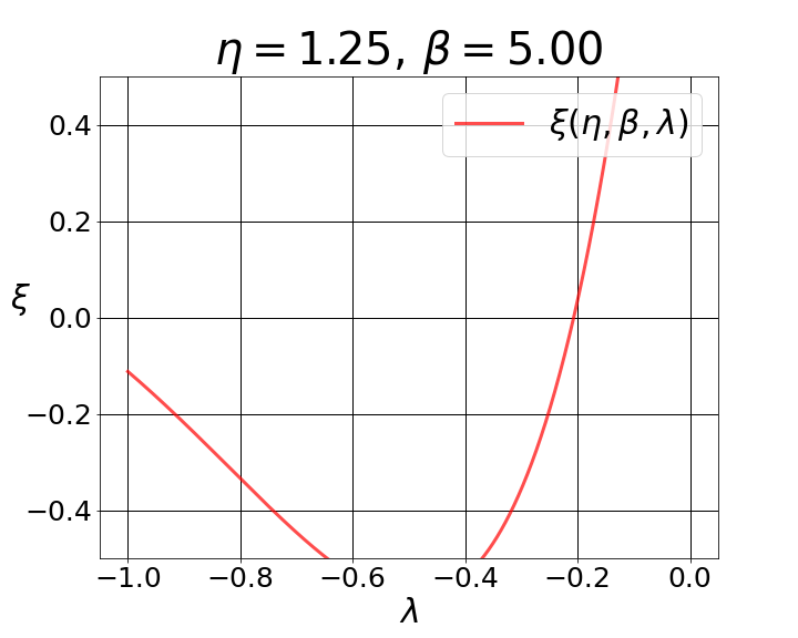
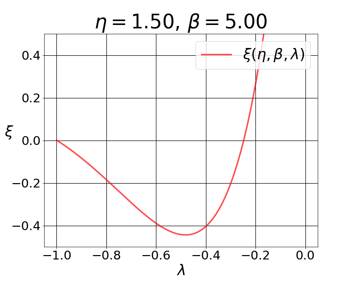
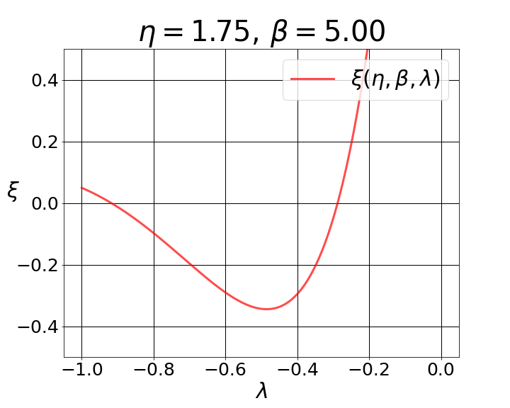
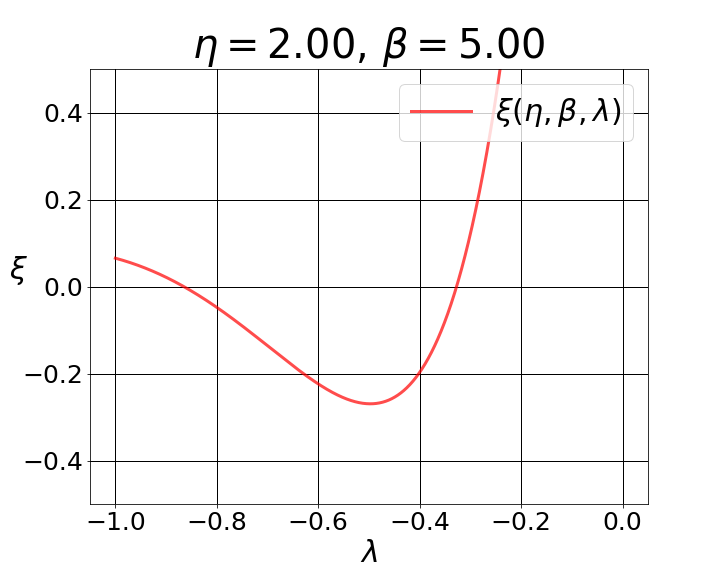
Figure 1: Plots of $\xi(\eta,\beta,\lambda)$ for various values of $\eta,\beta$

Choice of the parameter $\lambda$.

We will now prove that the parameter $\lambda$ is uniquely determined in a neighbourhood of $\eta=0$ by requiring that the solution $v=v(z,\eta,\beta)$ depends continuously on the parameter $\eta$.

Lemma 5.5.

There exists an $\varepsilon>0$ such that for all $\eta\in(-\varepsilon,\varepsilon)$ and $\beta>0$ there is a unique $\lambda=\lambda(\eta,\beta)$ such that $\xi(\eta,\beta,\lambda(\eta,\beta))=0$.

Proof.

When $\eta=0$ the matrix $R_{j}=\begin{pmatrix}1&0\\ 1&0\end{pmatrix}$ so that the only solution of the equation (5.28) $\xi(\eta=0,\beta,\lambda)=0$ is $\lambda=0$. To show the existence of the solution (5.28) for $\lambda=\lambda(\eta,\beta)$ near $\eta=0$, we use the implicit function theorem. We have to show that $\partial_{\lambda}\xi(\eta,\beta,\lambda)_{|_{(0,\beta,0)}}\neq 0$. For this purpose, we need to evaluate

$$\partial_{\lambda}\left(M_{k}\right)_{(\eta=0,\lambda=0)}=\begin{pmatrix}0&0\\ 0&0\end{pmatrix}\,,$$

where $M_{k}$ is defined in (5.25). This equation implies that

$$\partial_{\lambda}(\xi(\eta,\beta,\lambda))_{|_{(0,\beta,0)}}=\begin{pmatrix}1&0\end{pmatrix}\begin{pmatrix}1&0\\ 1&0\end{pmatrix}\begin{pmatrix}1\\ 0\end{pmatrix}=1.$$

Thus we can apply the implicit function theorem, and we obtain the claim. ∎

We conclude the proof of Theorem 2.3. When $\eta=0$ the only analytic solution of DCH equation is $v(z)=c$, $c\in{\mathbb{C}}\backslash\{0\}$. In this case, in principle $\lambda$ is undetermined. However, from Theorem 3.4 the minimizer $\mu^{\beta}_{HT}$ of (3.18) is the uniform measure on the circle and therefore from equation 5.14 one has $\lambda=0$. From Lemma 5.5 when $\eta\in(-\varepsilon,\varepsilon)$, there exists a unique $\lambda(\eta,\beta)$ that satisfies equation (5.28) and such that $\lambda(\eta=0,\beta)=0$ and therefore by Proposition 5.3 we obtain for $\eta\in(-\varepsilon,\varepsilon)$, the unique solution $v(z,\eta,\beta)$ of the DCH equation analytic in any compact set $|z|\leq r$, with $r>0$ and in particular when $r=1$. Because of lemma 5.2 the solution $v(z,\eta,\beta)$ is differentiable with respect to the parameters $\eta$ and $\beta$.

We remark that $v(z)\neq 0$ on the unit disc $\overline{{\mathbb{D}}}$ because of the relation (5.17) between the analytic function $G(z)$ and $v(z)$ and the uniqueness of the minimizer $\mu^{\beta}_{HT}$ and of the analytic solution $v(z)$ of (5.18).

To complete our proof of Theorem 2.3 we recover the explicit expression of $\mu^{\beta}_{HT}(\theta)$ from $G(z)$ and $v(z)$ using the Poisson representation formula (see for example [59, Chapter 1]):

$$\mu^{\beta}_{HT}(\theta)=-\frac{1}{2\pi}-\frac{\Re(iG(e^{i\theta}))}{\pi\beta}=\frac{1}{2\pi}+\frac{1}{\pi\beta}\Re\left.\left(\frac{zv^{\prime}(z)}{v(z)}\right|_{z=e^{i\theta}}\right)\,.$$ (5.35)

∎

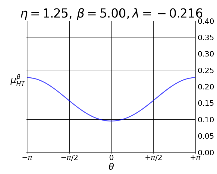
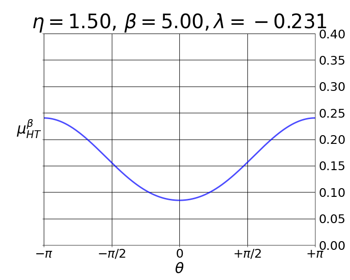
Figure 2: The mean density of states $\mu^{\beta}_{HT}$ for different parameters.

In Figure 2 we plotted the density of states of the Circular $\beta$ ensemble in the high-temperature regime with potential $V(z)=\eta\Re(z)$. To produce this picture and Figure 1, we used extensively the NumPy [38], and matplotlib [39] libraries.

Remark 5.6.

The Gross-Witten [35] and Baik-Deift-Johannson [11] solution is obtained by making the substitution $\eta\to\beta\eta$ and $\beta\to\infty$ in equation (3.18) which gives the functional

$${\mathcal{F}}^{(\eta)}(\mu):=\int\int\limits_{\mathbb{T}\times\mathbb{T}}\ln\left|\sin\left(\frac{\theta-\phi}{2}\right)\right|^{-1}\mu({\rm d}\theta)\mu({\rm d}\phi)+2\eta\int_{\mathbb{T}}\cos(\theta)\mu({\rm d}\theta).$$

The minimizer is $\mu(\theta)=\frac{1}{2\pi}\left(1-2\eta\cos\theta\right)$ with $0\leq 2\eta\leq 1$. In this case the first moment $\lambda=-\eta$.

Appendix A Proof of Proposition 4.2

First, we prove the relation between the free energies (4.3) namely:

$$\partial_{\beta}(\beta F_{HT}(V,\beta))+\ln(2)=F_{AL}(V,\beta)\,,$$ (A.1)

and we show that $F_{HT}(V,\beta)$ is analytic with respect to $\beta>0$.

From Remark 3.7, the above expression is equivalent to:

$$\partial_{\beta}\left(\beta\lim_{N\to\infty}\frac{\ln(Z^{HT}_{N}(V,\beta))}{N}\right)=\lim_{N\to\infty}\frac{\ln(Z^{AL}_{N}(V,\beta))}{N}\,.$$ (A.2)

To prove this relation, we will use the so-called transfer operator technique [41, 44, 56]. We are considering a potential of the form $\mbox{Tr}(V({\mathcal{E}}))$ as in (1.17) which is of finite range $K$, meaning that it can be expressed as a sum of local quantities, i.e. depending on a finite number $2K$ of variables, with $K$ independent of $N$ [54]. For example, if $V(z)=\Re(z)$, then $\mbox{Tr}({\mathcal{E}})=-2\sum_{j=1}^{N}\Re(\alpha_{j}{\overline{\alpha}}_{j+1})$ and in this case the range is $K=1$. Let $N=KM+L$ with $M,L\in{\mathbb{N}}$ and $L<K$. We split the coordinates $(\alpha_{1},\dots,\alpha_{N})$ into $M$ blocks of length $K$ and a reminder of length $L$, and we define the vector ${\widetilde{{\boldsymbol{\alpha}}}}_{j}$ of length $K$ as

$${\widetilde{{\boldsymbol{\alpha}}}}_{j}=(\alpha_{K(j-1)+1},\alpha_{K(j-1)+2},\ldots,\alpha_{Kj}).$$

In this notation,

$$(\alpha_{1},\dots,\alpha_{N})=(\overbrace{{\widetilde{{\boldsymbol{\alpha}}}}_{1},\dots,{\widetilde{{\boldsymbol{\alpha}}}}_{M}}^{KM},\overbrace{\alpha_{KM+1},\ldots,\alpha_{N}}^{L}),$$

$$\begin{split}\mbox{Tr}(V({\mathcal{E}}))&=\sum_{\ell=1}^{M-1}W({\widetilde{{\boldsymbol{\alpha}}}}_{\ell},{\widetilde{{\boldsymbol{\alpha}}}}_{\ell+1})+W({\widetilde{{\boldsymbol{\alpha}}}}_{M},\overbrace{\alpha_{KM+1},\ldots,\alpha_{KM+L}}^{L},\overbrace{\alpha_{1},\ldots,\alpha_{K-L}}^{K-L})\\ &+W_{1}(\overbrace{\alpha_{KM+1},\ldots,\alpha_{KM+L}}^{L},{\widetilde{{\boldsymbol{\alpha}}}}_{1}),\end{split}$$ (A.3)

where $W\,:\,\overline{{\mathbb{D}}}^{K}\times\overline{{\mathbb{D}}}^{K}\to{\mathbb{R}}$ and $W_{1}\,:\,\overline{{\mathbb{D}}}^{L}\times\overline{{\mathbb{D}}}^{K}\to{\mathbb{R}}$ are continuous functions. The last two terms in the above expression are different from the others since we may have an off-set of length $L$, due to periodicity. In the case $V(z)=\Re(z)$, then $W(\alpha_{1},\alpha_{2})=-2\Re(\alpha_{1}{\overline{\alpha}}_{2})$, there is no off-set and $W_{1}=0$.

For convenience, we define

$${\widetilde{{\boldsymbol{\alpha}}}}_{M+1}=(\alpha_{KM+1},\ldots,\alpha_{KM+L},\alpha_{1},\ldots,\alpha_{K-L}).$$

We can now rewrite $Z^{AL}_{N}(V,\beta)$ in (1.19) as

$$\begin{split}Z^{AL}_{N}(V,\beta)&=\int\limits_{{\mathbb{D}}^{N}}\prod_{j=1}^{N}\left(1-|\alpha_{j}|^{2}\right)^{\beta-1}\\ &\times\exp\left(-\sum_{\ell=1}^{M}W({\widetilde{{\boldsymbol{\alpha}}}}_{\ell},{\widetilde{{\boldsymbol{\alpha}}}}_{\ell+1}){-W_{1}(\alpha_{KM+1},\ldots,\alpha_{KM+L},{\widetilde{{\boldsymbol{\alpha}}}}_{1})}\right){\rm d}^{2}{\boldsymbol{\alpha}}\,.\end{split}$$ (A.4)

We are now in position to apply the transfer operator technique to compute this partition function. On $L^{2}({\mathbb{D}}^{K})$ we introduce the scalar product

$$\left(f,g\right)=\int_{{\mathbb{D}}^{K}}f({\bf z}){\overline{g({\bf z})}}{\rm d}{\bf z}\,,$$ (A.5)

where ${\bf z}=(z_{1},\ldots,z_{K})$. This scalar product induces a norm on $L^{2}({\mathbb{D}})$ and also a norm on bounded operators $T\;:\,L^{2}({\mathbb{D}}^{K})\to L^{2}({\mathbb{D}}^{K})$ as

$$||T||:=\sup_{f\,:\,||f||_{2}=1}||Tf||_{2}\,,$$ (A.6)

where $||f||_{2}$ is the standard $L^{2}$ norm.

Let $\boldsymbol{\zeta}=(\zeta_{1},\ldots,\ldots\zeta_{2K})$ with $\zeta_{K+j}=\zeta_{j}>0$ for $j=1,\dots,K$. We define the continuous family of transfer operators ${\mathcal{T}}_{\boldsymbol{\zeta}}\,:\,L^{2}({\mathbb{D}}^{K})\to L^{2}({\mathbb{D}}^{K})$ as

$$({\mathcal{T}}_{\boldsymbol{\zeta}}f)({\widetilde{{\boldsymbol{\alpha}}}}_{2})=\int_{{\mathbb{D}}^{K}}f({\widetilde{{\boldsymbol{\alpha}}}}_{1})\prod_{j=1}^{2K}\left(1-|\alpha_{j}|^{2}\right)^{\frac{\zeta_{j}-1}{2}}\exp\left(-W({\widetilde{{\boldsymbol{\alpha}}}}_{1},{\widetilde{{\boldsymbol{\alpha}}}}_{2})\right){\rm d}^{2}{\widetilde{{\boldsymbol{\alpha}}}}_{1}\,.$$ (A.7)

We observe that ${\mathcal{T}}_{\boldsymbol{\zeta}}$ is an integral operator whose kernel $\prod_{j=1}^{2K}\left(1-|\alpha_{j}|^{2}\right)^{\frac{\zeta_{j}-1}{2}}\exp\left(-W({\widetilde{{\boldsymbol{\alpha}}}}_{1},{\widetilde{{\boldsymbol{\alpha}}}}_{2})\right)$ belongs to $L^{2}({\mathbb{D}}^{K}\times{\mathbb{D}}^{K})$, and therefore ${\mathcal{T}}_{\boldsymbol{\zeta}}$ is an Hilbert-Schimdt operator. We conclude that there exists a complete set of normalized eigenfunctions $\{\psi_{j}\}_{j\geq 1}$ with eigenvalues $\{\lambda_{j}\}_{j\geq 1}$ numbered so that $\{|\lambda_{j}|\}_{j\geq 1}$ is a non-increasing sequence such that:

$$({\mathcal{T}}_{\boldsymbol{\zeta}}\psi_{j})({\bf z},V,\boldsymbol{\zeta})=\lambda_{j}(V,\boldsymbol{\zeta})\psi_{j}({\bf z},V,\boldsymbol{\zeta})\,,$$ (A.8)

$$\sum_{n=1}^{\infty}{\overline{\psi}}_{n}({\bf z},V,\boldsymbol{\zeta})\psi_{n}({\bf z}^{\prime},V,\boldsymbol{\zeta})=\delta_{\bf z}({\bf z}^{\prime})\,,$$ (A.9)

where $\delta_{\bf z}(\cdot)$ is the Dirac delta function at ${\bf z}\in{\mathbb{D}}^{K}$.

For clearness, we collect a series of properties that the operator ${\mathcal{T}}_{\boldsymbol{\zeta}}$ fulfils:

• $\sum_{j=1}^{\infty}|\lambda_{j}(V,\boldsymbol{\zeta})|^{2}<\infty$ and ${\mathcal{T}}_{\boldsymbol{\zeta}}$ is compact, since it is Hilbert-Schimdt (see [40, Chapter V.2.4]);

• The eigenvalue $\lambda_{1}(\boldsymbol{\zeta},V)$ is simple, positive and $\lambda_{1}(\boldsymbol{\zeta},V)>|\lambda_{n}(\boldsymbol{\zeta},V)|$ for all $n\geq 2$ (see [69, Theorem 137.4]);

• The eigenvalue $\lambda_{1}(\boldsymbol{\zeta},V)$ and its eigenfunction $\psi_{1}({\bf z},\boldsymbol{\zeta},V)$ are analytic functions of the parameters $\boldsymbol{\zeta}$, and for any real polynomial $P$ there exists an $\varepsilon>0$ such that the maps $t\to\lambda_{1}(\boldsymbol{\zeta},V+tP)$, $t\to\psi_{1}({\bf z},\boldsymbol{\zeta},V+tP)$ are analytic for $|t|<\varepsilon$ (see [40, Chapter VII, Theorem 1.8]).

We artificially rewrite $Z^{AL}_{N}(V,\beta)$ in (A.4) as

$$\begin{split}&Z^{AL}_{N}(V,\beta)=\int\limits_{{\mathbb{D}}^{N+K}}\delta_{{\widetilde{{\boldsymbol{\alpha}}}}_{1}}({\boldsymbol{\gamma}})\prod_{\ell=1}^{K}\left[\left(1-|\gamma_{\ell}|^{2}\right)\left(1-|\alpha_{\ell}|^{2}\right)\right]^{\frac{\beta-1}{2}}\prod_{\ell=K+1}^{N}\left(1-|\alpha_{\ell}|^{2}\right)^{\beta-1}\\ &\times\exp\left(-\sum_{\ell=1}^{M-1}W({\widetilde{{\boldsymbol{\alpha}}}}_{\ell},{\widetilde{{\boldsymbol{\alpha}}}}_{\ell+1})-W({\widetilde{{\boldsymbol{\alpha}}}}_{M},\alpha_{KM+1},\ldots,\alpha_{N},\gamma_{1},\ldots,\gamma_{K-L})\right)\\ &\times\exp\left(-W_{1}(\alpha_{KM+1},\ldots,\alpha_{KM+L},{\boldsymbol{\gamma}})\right)\prod_{j=1}^{N}{\rm d}^{2}\alpha_{j}{\rm d}^{2}{\boldsymbol{\gamma}}\,,\end{split}$$ (A.10)

where ${\boldsymbol{\gamma}}=(\gamma_{1},\ldots,\gamma_{K})$ and ${\boldsymbol{\gamma}}\in{\mathbb{D}}^{K}$.
We can use (A.9) with $\boldsymbol{\zeta}=\boldsymbol{\beta}=\overbrace{(\beta,\dots,\beta)}^{2K}$ to rewrite the previous equation as:

$$\begin{split}&Z^{AL}_{N}(V,\beta)=\int\limits_{{\mathbb{D}}^{N+K}}\sum_{n=1}^{\infty}{\overline{\psi}}_{n}({\boldsymbol{\gamma}},V,\boldsymbol{\beta})\psi_{n}({\widetilde{{\boldsymbol{\alpha}}}}_{1},V,\boldsymbol{\beta})\\ &\times\prod_{\ell=1}^{K}\left[\left(1-|\gamma_{\ell}|^{2}\right)\left(1-|\alpha_{\ell}|^{2}\right)\right]^{\frac{\beta-1}{2}}\prod_{\ell=K+1}^{N}\left(1-|\alpha_{\ell}|^{2}\right)^{\beta-1}\\ &\times\exp\left(-\sum_{\ell=1}^{M-1}W({\widetilde{{\boldsymbol{\alpha}}}}_{\ell},{\widetilde{{\boldsymbol{\alpha}}}}_{\ell+1})-W({\widetilde{{\boldsymbol{\alpha}}}}_{M},\alpha_{KM+1},\ldots,\alpha_{N},\gamma_{1},\ldots,\gamma_{K-L})\right)\\ &\times\exp\left(-W_{1}(\alpha_{KM+1},\ldots,\alpha_{KM+L},{\boldsymbol{\gamma}})\right){\rm d}^{2}{\boldsymbol{\alpha}}{\rm d}^{2}{\boldsymbol{\gamma}}\\ &=\sum_{n=1}^{\infty}\int_{{\mathbb{D}}^{N}}{\overline{\psi}}_{n}({\boldsymbol{\gamma}},V,\boldsymbol{\beta})({\mathcal{T}}_{\boldsymbol{\beta}}\psi_{n})({\widetilde{{\boldsymbol{\alpha}}}}_{2})\prod_{\ell=K+1}^{2K}\left(1-|\alpha_{\ell}|^{2}\right)^{\frac{\beta-1}{2}}\prod_{\ell=2K+1}^{N}\left(1-|\alpha_{\ell}|^{2}\right)^{\beta-1}\\ &\times\exp\left(-\sum_{\ell=2}^{M-1}W({\widetilde{{\boldsymbol{\alpha}}}}_{\ell},{\widetilde{{\boldsymbol{\alpha}}}}_{\ell+1})-W({\widetilde{{\boldsymbol{\alpha}}}}_{M},\alpha_{KM+1},\ldots,\alpha_{N},\gamma_{1},\ldots,\gamma_{K-L})\right)\\ &\times\exp\left(-W_{1}(\alpha_{KM+1},\ldots,\alpha_{KM+L},{\boldsymbol{\gamma}})\right)\prod_{\ell=1}^{K}{\rm d}^{2}\gamma_{\ell}\left(1-|\gamma_{\ell}|^{2}\right)^{\frac{\beta-1}{2}}\prod_{\ell=K+1}^{N}{\rm d}^{2}\alpha_{\ell}\\ &=\sum_{n=1}^{\infty}\lambda_{n}(V,\boldsymbol{\beta})\int_{{\mathbb{D}}^{N}}{\overline{\psi}}_{n}({\boldsymbol{\gamma}},V,\boldsymbol{\beta})\psi_{n}({\widetilde{{\boldsymbol{\alpha}}}}_{2},V,\boldsymbol{\beta})\prod_{\ell=K+1}^{2K}\left(1-|\alpha_{\ell}|^{2}\right)^{\frac{\beta-1}{2}}\\ &\prod_{\ell=2K+1}^{N}\left(1-|\alpha_{\ell}|^{2}\right)^{\beta-1}\exp\left(-\sum_{\ell=2}^{M-1}W({\widetilde{{\boldsymbol{\alpha}}}}_{\ell},{\widetilde{{\boldsymbol{\alpha}}}}_{\ell+1})\right)\\ &\times\exp\left(-W({\widetilde{{\boldsymbol{\alpha}}}}_{M},\alpha_{KM+1},\ldots,\alpha_{N},\gamma_{1},\ldots,\gamma_{K-L})\right)\\ &\times\exp\left(-W_{1}(\alpha_{KM+1},\ldots,\alpha_{KM+L},{\boldsymbol{\gamma}})\right)\prod_{\ell=1}^{K}{\rm d}^{2}\gamma_{\ell}\left(1-|\gamma_{\ell}|^{2}\right)^{\frac{\beta-1}{2}}\prod_{\ell=K+1}^{N}{\rm d}^{2}\alpha_{\ell}\,.\end{split}$$ (A.11)

In the above integral, from the first to the second relation we identify the integral operator ${\mathcal{T}}_{\boldsymbol{\beta}}$ where $\boldsymbol{\beta}=\overbrace{(\beta,\dots,\beta)}^{2K}$. We repeatedly apply ${\mathcal{T}}_{\boldsymbol{\beta}}$ and (A.8) another $M-2$ times to the above integral, to obtain:

$$Z^{AL}_{N}(V,\beta)=\sum_{n=1}^{\infty}(\lambda_{n}(V,\boldsymbol{\beta}))^{M-1}R_{n},$$ (A.12)

$$R_{n}=\int_{{\mathbb{D}}^{2K+L}}\overline{\psi}_{n}({\boldsymbol{\gamma}},V,\boldsymbol{\beta})\psi_{n}({\widetilde{{\boldsymbol{\alpha}}}}_{M},V,\boldsymbol{\beta})\prod_{\ell=1}^{K}{\rm d}^{2}\gamma_{\ell}\left(1-|\gamma_{\ell}|^{2}\right)^{\frac{\beta-1}{2}}$$ (A.13)

$$\prod_{\ell=(M-1)K+1}^{MK}\left(1-|\alpha_{\ell}|^{2}\right)^{\frac{\beta-1}{2}}\prod_{\ell=MK+1}^{N}\left(1-|\alpha_{\ell}|^{2}\right)^{\beta-1}$$

$$\times\exp\left(-W({\widetilde{{\boldsymbol{\alpha}}}}_{M},\alpha_{KM+1},\ldots,\alpha_{N},\gamma_{1},\ldots,\gamma_{K-L})\right)$$

$$\times\exp\left(-W_{1}(\alpha_{KM+1},\ldots,\alpha_{KM+L},{\boldsymbol{\gamma}})\right)\prod_{\ell=(M-1)K+1}^{N}{\rm d}^{2}\alpha_{\ell}.$$

The modulus of the reminder $|R_{n}|$ in (A.13) can be easily bounded from above and below by two constants $C_{1},C_{2}>0$ independent of $N$, therefore we conclude from (A.12) that

$$F_{AL}(V,\beta)=-\lim_{N\to\infty}\frac{1}{N}\ln\left(Z^{AL}_{N}(V,\beta)\right)=-\frac{1}{K}\ln\left(\lambda_{1}(V,\boldsymbol{\beta})\right)\,.$$ (A.14)

Since $\lambda_{1}(V,\boldsymbol{\beta})$ is analytic for $\beta>0$, see [40, Chapter VII, Theorem 1.8], and strictly positive, see [69, Theorem 137.4], we conclude that $F_{AL}(V,\beta)$ is analytic with respect to $\beta$.

We can apply the same procedure to the partition function $Z^{HT}_{N}(V,\beta)$ in (3.8). Also in this case the potential $\mbox{Tr}(V({\widetilde{E}}))$ with $V$ as in (1.17) and the matrix ${\widetilde{E}}$ as in (3.7) is of finite range $K$, meaning that it can be expressed as a sum of local quantities [54]. More precisely, assuming $N=KM+L$ with $L<K$ and $M,N,L\in{\mathbb{N}}$ we have

$$\begin{split}\mbox{Tr}(V({\widetilde{E}}))&=\sum_{\ell=1}^{M-1}W({\widetilde{{\boldsymbol{\alpha}}}}_{\ell},{\widetilde{{\boldsymbol{\alpha}}}}_{\ell+1})+W(\overbrace{0,\ldots,0}^{K-1},-1,{\widetilde{{\boldsymbol{\alpha}}}}_{1})\\ &+W({\widetilde{{\boldsymbol{\alpha}}}}_{M},\underbrace{\alpha_{KM+1},\ldots,\alpha_{N}}_{L},\underbrace{0,\dots,0}_{K-L})\,.\end{split}$$ (A.15)

For example for $V(z)=z^{2}+\bar{z}^{2}$ one has $K=2$ and $N=2M+L$ where $L=0,1$, depending on the parity of $N$. The vector ${\widetilde{{\boldsymbol{\alpha}}}}_{\ell}$ takes the form ${\widetilde{{\boldsymbol{\alpha}}}}_{\ell}=(\alpha_{2\ell-1},\alpha_{2\ell})$ for $\ell=1,\dots,M$. In this notation, we can rewrite the potential as

$$\mbox{Tr}(V({\widetilde{E}}))=\sum_{\ell=1}^{M-1}W({\widetilde{{\boldsymbol{\alpha}}}}_{\ell},{\widetilde{{\boldsymbol{\alpha}}}}_{\ell+1})+W({\widetilde{{\boldsymbol{\alpha}}}}_{M},\delta_{L,1}\alpha_{N},0)+\underbrace{2\Re(\alpha_{1}^{2}+2\bar{\alpha}_{2}\rho_{1}^{2})}_{=W(0,-1,\alpha_{1},\alpha_{2})}\,,$$ (A.16)

where in this case

$$W({\widetilde{{\boldsymbol{\alpha}}}}_{\ell},{\widetilde{{\boldsymbol{\alpha}}}}_{\ell+1})=2\Re\sum_{s=0}^{1}(\alpha_{2\ell-1+s}\bar{\alpha}_{2\ell+s})^{2}-4\Re\sum_{s=0}^{1}\alpha_{2\ell-1+s}\bar{\alpha}_{2\ell+1+s}\rho_{2\ell+s}^{2}$$

and $\delta_{L,1}$ is equal to zero for $L\neq 1$.
Using (A.15) the partition function can be written in the form

$$\begin{split}Z^{HT}_{N}(V,\beta)&=\int\limits_{{\mathbb{D}}^{N-1}\times S^{1}}\frac{{\rm d}\alpha_{N}}{i\alpha_{N}}\prod_{j=1}^{N-1}{\rm d}^{2}\alpha_{j}\left(1-|\alpha_{j}|^{2}\right)^{\beta\left(1-\frac{j}{N}\right)-1}\\ &\times\exp\left(-\sum_{\ell=1}^{M-1}W({\widetilde{{\boldsymbol{\alpha}}}}_{\ell},{\widetilde{{\boldsymbol{\alpha}}}}_{\ell+1})-W({\widetilde{{\boldsymbol{\alpha}}}}_{M},\alpha_{KM+1},\ldots,\alpha_{N},\overbrace{0,\dots,0}^{K-L})\right)\\ &\times\exp\left(-W(\overbrace{0,\ldots,0}^{K-1},-1,{\widetilde{{\boldsymbol{\alpha}}}}_{1})\right)\,.\end{split}$$ (A.17)

We want to apply the same technique as in the previous case, but we have to pay attention to one important detail: in this situation, the eigenvalues and the eigenfunctions of the transfer operators will be dependent on the block number. Indeed, in this case, the exponents of $(1-|\alpha_{j}|^{2})$ are not identical, but they depend on the index $j$ as in (A.17).

For this reason, we define

$$\boldsymbol{\zeta}^{(1)}=\beta\overbrace{\left(1-\frac{1}{N},1-\frac{2}{N}\,\ldots,1-\frac{K}{N},1-\frac{1}{N},1-\frac{2}{N},\ldots,1-\frac{K}{N}\right)}^{2K}\,,$$

and

$$\boldsymbol{\zeta}^{(j)}=\boldsymbol{\zeta}^{(1)}-\beta\frac{j-1}{N}\boldsymbol{K},\quad j=1,\dots,M-1\,,$$

where the vector $\boldsymbol{K}$ has entries $\boldsymbol{K}_{j}=K$ for $j=1,\dots,2K$. For $K$ integer and $K<N$ we introduce the multiplication operator ${\mathcal{M}}_{K}:L^{2}({\mathbb{D}}^{K})\to L^{2}({\mathbb{D}}^{K})$ defined as

$$({\mathcal{M}}_{K}f)({\boldsymbol{\alpha}})=\prod_{j=1}^{K}\left(1-|\alpha_{j}|^{2}\right)^{-\frac{K\beta}{2N}}f({\boldsymbol{\alpha}}).$$

Remark A.1.

We notice that, for $\beta\in{\mathbb{R}}$, $K\in{\mathbb{N}}$ and $N\in{\mathbb{N}}$ big enough, the function $\prod_{j=1}^{K}\left(1-|\alpha_{j}|^{2}\right)^{-\frac{K\beta}{2N}}\in L^{2}({\mathbb{D}}^{K})$. Since we are considering the limit $N\to\infty$, and $\beta,K$ independent from $N$, we always assume that this condition holds.

We observe that ${\mathcal{M}}_{-K}=({\mathcal{M}}_{K})^{-1}$ and the operators ${\mathcal{T}}_{\boldsymbol{\zeta}^{(j)}}:L^{2}({\mathbb{D}}^{K})\to L^{2}({\mathbb{D}}^{K})$ defined in (A.7) satisfy the relation

$${\mathcal{T}}_{\boldsymbol{\zeta}^{(j+1)}}={\mathcal{M}}_{K}{\mathcal{T}}_{\boldsymbol{\zeta}^{(j)}}{\mathcal{M}}_{K},\quad j=1,\dots,M-1.$$ (A.18)

We recall that the operators ${\mathcal{T}}_{\boldsymbol{\zeta}^{(j)}}$ are compact, furthermore, we notice that ${\mathcal{M}}_{K}{\mathcal{T}}_{\boldsymbol{\zeta}^{(j)}}$ is also compact since it is Hilbert–Schmidt [40].

Let us define the $K(M-1)$-dimensional vector $\boldsymbol{\zeta}_{M}=(\boldsymbol{\zeta}^{(M-1)},\dots,\boldsymbol{\zeta}^{(1)})$ and the operator ${\widetilde{{\mathcal{T}}}}_{M,\boldsymbol{\zeta}_{M}}:L^{2}({\mathbb{D}}^{K})\to L^{2}({\mathbb{D}}^{K})$ as

$${\widetilde{{\mathcal{T}}}}_{M,\boldsymbol{\zeta}_{M}}={\mathcal{M}}_{K}{\mathcal{T}}_{\boldsymbol{\zeta}^{(M-1)}}{\mathcal{M}}_{K}{\mathcal{T}}_{\boldsymbol{\zeta}^{(M-2)}}{\mathcal{M}}_{K}\cdots{\mathcal{M}}_{K}{\mathcal{T}}_{\boldsymbol{\zeta}^{(1)}}\,,$$ (A.19)

we notice that it is a compact operator, since all ${\mathcal{M}}_{K}{\mathcal{T}}_{\boldsymbol{\zeta}^{(j)}}$ are Hilbert–Schmidt.

We will now prove the following technical result:

Proposition A.2.

Let ${\widetilde{{\mathcal{T}}}}_{M,\boldsymbol{\zeta}_{M}}$ as in (A.19) and $Z_{N}^{HT}$ as in (A.17) then:

$$\lim_{N\to\infty}\frac{1}{N}\ln\left(\frac{Z_{N}^{HT}}{\mbox{Tr}({\widetilde{{\mathcal{T}}}}_{M,\boldsymbol{\zeta}_{M}})}\right)=0\,,$$ (A.20)

here by $\mbox{Tr}({\widetilde{{\mathcal{T}}}}_{M,\boldsymbol{\zeta}_{M}})$ we indicate the standard trace on $L^{2}$.

Proof.

We will estimate both $Z_{N}^{HT}$, and $\mbox{Tr}({\widetilde{{\mathcal{T}}}}_{M,\boldsymbol{\zeta}_{M}})$ from above and below, then combining these estimates we will obtain (A.20). We start with $Z_{N}^{HT}$.

$$\begin{split}Z_{N}^{HT}&=\int\limits_{{\mathbb{D}}^{N-1}\times S^{1}}\frac{{\rm d}\alpha_{N}}{i\alpha_{N}}\left[\prod_{j=1}^{N-1}{\rm d}^{2}\alpha_{j}\left(1-|\alpha_{j}|^{2}\right)^{\beta\left(1-\frac{j}{N}\right)-1}\right]\\ &\times\exp\left(-\sum_{\ell=1}^{M-1}W({\widetilde{{\boldsymbol{\alpha}}}}_{\ell},{\widetilde{{\boldsymbol{\alpha}}}}_{\ell+1})-W({\widetilde{{\boldsymbol{\alpha}}}}_{M},\alpha_{KM+1},\ldots,\alpha_{N},\overbrace{0,\dots,0}^{K-L})\right)\\ &\times\exp\left(-W(\overbrace{0,\ldots,0}^{K-1},-1,{\widetilde{{\boldsymbol{\alpha}}}}_{1})\right)\,.\end{split}$$ (A.21)

We can bound the first and the last three terms in the above exponential with two positive constants $C(V,\beta)$ and $c(V,\beta)$, independent of $N$, such that

$$\begin{split}c(V,\beta)&\leq\exp\left(-W({\widetilde{{\boldsymbol{\alpha}}}}_{1},{\widetilde{{\boldsymbol{\alpha}}}}_{2})-W({\widetilde{{\boldsymbol{\alpha}}}}_{M-1},{\widetilde{{\boldsymbol{\alpha}}}}_{M})-W({\widetilde{{\boldsymbol{\alpha}}}}_{M},\alpha_{KM+1},\ldots,\alpha_{N},\overbrace{0,\dots,0}^{K-L})\right)\\ &\times\exp\left(-W(\overbrace{0,\ldots,0}^{K-1},-1,{\widetilde{{\boldsymbol{\alpha}}}}_{1})\right)\leq C(V,\beta)\,\end{split}$$ (A.22)

where in the exponents each $\alpha_{j}\in\overline{\mathbb{D}}$. From the previous inequalities, we deduce that the integral

$$\int\limits_{{\mathbb{D}}^{N-1}\times S^{1}}\frac{{\rm d}\alpha_{N}}{i\alpha_{N}}\left[\prod_{j=1}^{N-1}{\rm d}^{2}\alpha_{j}\left(1-|\alpha_{j}|^{2}\right)^{\beta\left(1-\frac{j}{N}\right)-1}\right]\exp\left(-\sum_{\ell=2}^{M-2}W({\widetilde{{\boldsymbol{\alpha}}}}_{\ell},{\widetilde{{\boldsymbol{\alpha}}}}_{\ell+1})\right)$$ (A.23)

is bounded from above by $Z_{N}^{HT}/c(V,\beta)$ and from below by $Z_{N}^{HT}/C(V,\beta)$. We can explicitly integrate in $\alpha_{j}$ for $j=1,\ldots,K$ and $j=(M-1)K+1,\ldots,N$ using the formula

$$\int_{\mathbb{D}}\left(1-|z|^{2}\right)^{t-1}{\rm d}^{2}z=\pi t^{-1}\,,$$ (A.24)

obtaining that there are two constants $C_{1}(V,\beta)$ and $c_{1}(V,\beta)$ depending on $V,\,\beta,K$ and $L$ but not on $N$, such that

$$\begin{split}Z_{N}^{HT}&\leq C_{1}(V,\beta)N^{K+L-1}\int\limits_{{\mathbb{D}}^{(M-2)K}}\left[\prod_{j=K+1}^{(M-1)K}{\rm d}^{2}\alpha_{j}\left(1-|\alpha_{j}|^{2}\right)^{\beta\left(1-\frac{j}{N}\right)-1}\right]\\ &\times\exp\left(-\sum_{\ell=2}^{M-2}W({\widetilde{{\boldsymbol{\alpha}}}}_{\ell},{\widetilde{{\boldsymbol{\alpha}}}}_{\ell+1})\right)\,,\end{split}$$ (A.25)

and

$$\begin{split}Z_{N}^{HT}&\geq c_{1}(V,\beta)N^{K+L-1}\int\limits_{{\mathbb{D}}^{(M-2)K}}\left[\prod_{j=K+1}^{(M-1)K}{\rm d}^{2}\alpha_{j}\left(1-|\alpha_{j}|^{2}\right)^{\beta\left(1-\frac{j}{N}\right)-1}\right]\\ &\times\exp\left(-\sum_{\ell=2}^{M-2}W({\widetilde{{\boldsymbol{\alpha}}}}_{\ell},{\widetilde{{\boldsymbol{\alpha}}}}_{\ell+1})\right)\,.\end{split}$$ (A.26)

We can proceed analogously to estimate the trace of ${\widetilde{{\mathcal{T}}}}_{M,\boldsymbol{\zeta}_{M}}$:

$$\begin{split}\mbox{Tr}({\widetilde{{\mathcal{T}}}}_{M,\boldsymbol{\zeta}_{M}})&=\int\limits_{{\mathbb{D}}^{(M-1)K}}\prod_{j=1}^{K}\left(1-|\alpha_{j}|^{2}\right)^{\frac{\beta}{2}\left(1-\frac{j}{N}\right)-\frac{1}{2}}\prod_{j=1}^{K}\left(1-|\alpha_{j}|^{2}\right)^{\frac{\beta}{2}\left(1-\frac{(M-1)K+j}{N}\right)-\frac{1}{2}}\\ &\times\prod_{j=K+1}^{(M-1)K}\left(1-|\alpha_{j}|^{2}\right)^{\beta\left(1-\frac{j}{N}\right)-1}\\ &\times\exp\left(-\sum_{j=1}^{M-2}W({\widetilde{{\boldsymbol{\alpha}}}}_{j},{\widetilde{{\boldsymbol{\alpha}}}}_{j+1})-W({\widetilde{{\boldsymbol{\alpha}}}}_{M-1},{\widetilde{{\boldsymbol{\alpha}}}}_{1})\right)\times\prod_{j=1}^{(M-1)K}{\rm d}^{2}\alpha_{j}\,.\end{split}$$ (A.27)

As before, we notice that there exist two positive constants ${\widetilde{C}}(V,\beta)$, and ${\widetilde{c}}(V,\beta)$, independent of $N$, such that

$${\widetilde{c}}(V,\beta)<\exp\left(-W({\widetilde{{\boldsymbol{\alpha}}}}_{1},{\widetilde{{\boldsymbol{\alpha}}}}_{2})-W({\widetilde{{\boldsymbol{\alpha}}}}_{M-1},{\widetilde{{\boldsymbol{\alpha}}}}_{1})\right)<{\widetilde{C}}(V,\beta)\,$$ (A.28)

when ${\boldsymbol{\alpha}}_{1},{\boldsymbol{\alpha}}_{2},{\boldsymbol{\alpha}}_{M-1}\in\overline{\mathbb{D}^{K}}$. From these inequalities, we deduce that the integral

$$\begin{split}&\int\limits_{{\mathbb{D}}^{(M-1)K}}\prod_{j=1}^{K}\left(1-|\alpha_{j}|^{2}\right)^{\frac{\beta}{2}\left(1-\frac{j}{N}\right)-\frac{1}{2}}\prod_{j=1}^{K}\left(1-|\alpha_{j}|^{2}\right)^{\frac{\beta}{2}\left(1-\frac{(M-1)K+j}{N}\right)-\frac{1}{2}}\\ &\times\prod_{j=K+1}^{(M-1)K}\left(1-|\alpha_{j}|^{2}\right)^{\beta\left(1-\frac{j}{N}\right)-1}\exp\left(-\sum_{j=2}^{M-2}W({\widetilde{{\boldsymbol{\alpha}}}}_{j},{\widetilde{{\boldsymbol{\alpha}}}}_{j+1})\right)\prod_{j=1}^{(M-1)K}{\rm d}^{2}\alpha_{j}\end{split}$$ (A.29)

is bounded from above by $\mbox{Tr}({\widetilde{{\mathcal{T}}}}_{M,\boldsymbol{\zeta}_{M}})/{\widetilde{c}}(V,\beta)$ and from below by $\mbox{Tr}({\widetilde{{\mathcal{T}}}}_{M,\boldsymbol{\zeta}_{M}})/{\widetilde{C}}(V,\beta)$. Using (A.24) we can now explicitly integrate in $\alpha_{j}$ for $j=1,\ldots,K$ the above integral obtaining the following inequalities

$$\begin{split}\mbox{Tr}({\widetilde{{\mathcal{T}}}}_{M,\boldsymbol{\zeta}_{M}})&\leq{\widetilde{C}}_{1}(V,\beta)\int\limits_{{\mathbb{D}}^{(M-2)K}}\left[\prod_{j=K+1}^{(M-1)K}{\rm d}^{2}\alpha_{j}\left(1-|\alpha_{j}|^{2}\right)^{\beta\left(1-\frac{j}{N}\right)-1}\right]\\ &\times\exp\left(-\sum_{\ell=2}^{M-2}W({\widetilde{{\boldsymbol{\alpha}}}}_{\ell},{\widetilde{{\boldsymbol{\alpha}}}}_{\ell+1})\right)\,,\end{split}$$ (A.30)

$$\begin{split}\mbox{Tr}({\widetilde{{\mathcal{T}}}}_{M,\boldsymbol{\zeta}_{M}})&\geq{\widetilde{c}}_{1}(V,\beta)\int\limits_{{\mathbb{D}}^{(M-2)K}}\left[\prod_{j=K+1}^{(M-1)K}{\rm d}^{2}\alpha_{j}\left(1-|\alpha_{j}|^{2}\right)^{\beta\left(1-\frac{j}{N}\right)-1}\right]\\ &\times\exp\left(-\sum_{\ell=2}^{M-2}W({\widetilde{{\boldsymbol{\alpha}}}}_{\ell},{\widetilde{{\boldsymbol{\alpha}}}}_{\ell+1})\right)\,,\end{split}$$ (A.31)

where ${\widetilde{C}}_{1}(V,\beta)$, and ${\widetilde{c}}_{1}(V,\beta)$ are positive constants depending on $V,\,\beta,K$ and $L$ but not on $N$. Combining (A.25)-(A.26)-(A.30)-(A.31) we deduce (A.20). ∎

Applying the previous proposition, we can express the Free energy of the Circular $\beta$ ensemble in the high-temperature regime in terms of $\mbox{Tr}({\widetilde{{\mathcal{T}}}}_{M})$:

$$\begin{split}F_{HT}(V,\beta)&=-\lim_{N\to\infty}\frac{1}{N}\ln\left(Z_{N}^{HT}\right)\\ &=-\lim_{N\to\infty}\frac{1}{N}\left(\ln\left(\frac{Z_{N}^{HT}}{\mbox{Tr}({\widetilde{{\mathcal{T}}}}_{M,\boldsymbol{\zeta}_{M}})}\right)+\ln(\mbox{Tr}({\widetilde{{\mathcal{T}}}}_{M,\boldsymbol{\zeta}_{M}}))\right)\\ &=-\lim_{N\to\infty}\frac{\ln(\mbox{Tr}({\widetilde{{\mathcal{T}}}}_{M,\boldsymbol{\zeta}_{M}}))}{N}\,,\end{split}$$ (A.32)

where in the last equality we used Proposition A.2.

As a final step, we have to understand the behaviour of $\mbox{Tr}({\widetilde{{\mathcal{T}}}}_{M,\boldsymbol{\zeta}_{M}})$, and for this purpose we need to carefully analyse the compact operators ${\mathcal{T}}_{\boldsymbol{\zeta}^{(j)}}$.

Let $\{\psi_{n}({\bf z},V,\boldsymbol{\zeta}^{(j)})\}_{n\geq 1}$ be the eigenfunctions of ${\mathcal{T}}_{\boldsymbol{\zeta}^{(j)}}$ with corresponding eigenvalues $\{\lambda_{n}(V,\boldsymbol{\zeta}^{(j)})\}_{n\geq 1}$ and $|\lambda_{1}(V,\boldsymbol{\zeta}^{(j)})|\geq|\lambda_{2}(V,\boldsymbol{\zeta}^{(j)})|\geq\dots$. From a generalized version of Jentzsch’s Theorem (see [69, Theorem 137.4]), we deduce that $|\lambda_{n}(V,\boldsymbol{\zeta}^{(j)})|<\lambda_{1}(V,\boldsymbol{\zeta}^{(j)})$ for all $n\geq 2$.

We are now in the position to prove the following proposition.

Proposition A.3.

Let $\{\psi_{n}({\bf z},V,\boldsymbol{\zeta}^{(j)})\}_{n=1}^{\infty}$ be the eigenfunctions of the operator ${\mathcal{T}}_{\boldsymbol{\zeta}^{(j)}}$ in (A.7) with corresponding eigenvalues $\{\lambda_{n}(V,\boldsymbol{\zeta}^{(j)})\}_{n=1}^{\infty}$. Consider the operator ${\widetilde{{\mathcal{T}}}}_{M,\boldsymbol{\zeta}_{M}}$ in (A.19), then there are constants ${\mathtt{d}},a_{j},c_{j}$, $j=1,\ldots,M-1$ uniformly bounded in $N$, and so in $M$, such that :

$$\left(\psi_{1}({\bf z},V,\boldsymbol{\zeta}^{(1)}),{\widetilde{{\mathcal{T}}}}_{M,\boldsymbol{\zeta}_{M}}\psi_{1}({\bf z},V,\boldsymbol{\zeta}^{(1)})\right)=\prod_{j=1}^{M-1}\lambda_{1}(V,\boldsymbol{\zeta}^{(j)})\left(1+\frac{a_{j}}{N}+O\left(\frac{1}{N^{2}}\right)\right)\,,$$ (A.33)

$$\left|\sum_{\ell\geq 2}\left(\psi_{\ell}({\bf z},V,\boldsymbol{\zeta}^{(1)}),{\widetilde{{\mathcal{T}}}}_{M,\boldsymbol{\zeta}_{M}}\psi_{\ell}({\bf z},V,\boldsymbol{\zeta}^{(1)})\right)\right|\leq{\mathtt{d}}\prod_{j=3}^{M-1}\lambda_{1}(V,\boldsymbol{\zeta}^{(j)})\left(1+\frac{c_{j}}{N}+O\left(\frac{1}{N^{2}}\right)\right)$$ (A.34)

Proof.

To simplify the notation, we will drop the $V$ dependence of the eigenvalues $\lambda_{n}(V,\boldsymbol{\zeta}^{(j)})$, and of the eigenfunctions $\psi_{n}({\bf z},V,\boldsymbol{\zeta}^{(j)})$.

We will prove (A.33) by induction on $M$. For $M=2$, we have that ${\widetilde{{\mathcal{T}}}}_{M,\boldsymbol{\zeta}_{M}}={\mathcal{M}}_{K}{\mathcal{T}}_{\boldsymbol{\zeta}^{(1)}}$, so we have to compute:

$$\begin{split}&\bigg{(}\psi_{1}({\bf z},\boldsymbol{\zeta}^{(1)}),{\mathcal{M}}_{K}{\mathcal{T}}_{\boldsymbol{\zeta}^{(1)}}\psi_{1}({\bf z},\boldsymbol{\zeta}^{(1)})\bigg{)}=\lambda_{1}(\boldsymbol{\zeta}^{(1)})\left(\psi_{1}({\bf z},\boldsymbol{\zeta}^{(1)}),{\mathcal{M}}_{K}\psi_{1}({\bf z},\boldsymbol{\zeta}^{(1)})\right)\\ &\qquad=\lambda_{1}(\boldsymbol{\zeta}^{(1)})\left(\psi_{1}({\bf z},\boldsymbol{\zeta}^{(1)}),\prod_{j=1}^{K}(1-|z_{j}|^{2})^{-\frac{K\beta}{2N}}\psi_{1}({\bf z},\boldsymbol{\zeta}^{(1)})\right)\\ &\qquad=\lambda_{1}(\boldsymbol{\zeta}^{(1)})\left(\psi_{1}({\bf z},\boldsymbol{\zeta}^{(1)}),\left(1+\frac{{\widetilde{a}}_{1}({\bf z})}{N}+O\left(\frac{1}{N^{2}}\right)\right)\psi_{1}({\bf z},\boldsymbol{\zeta}^{(1)})\right)\\ &\qquad=\lambda_{1}(\boldsymbol{\zeta}^{(1)})\left(1+\frac{a_{1}}{N}+O\left(\frac{1}{N^{2}}\right)\right),\end{split}$$ (A.35)

where the function ${\widetilde{a}}_{1}({\bf z})$ is the first term of the expansion of $\prod_{j=1}^{K}(1-|z_{j}|^{2})^{-\frac{K\beta}{2N}}$ in powers of $1/N$ and the constant $a_{1}=\left(\psi_{1}({\bf z},\boldsymbol{\zeta}^{(1)}),{\widetilde{a}}_{1}({\bf z})\psi_{1}({\bf z},\boldsymbol{\zeta}^{(1)})\right)$ is uniformly bounded in $N$. So the first inductive step is proved.

For general $M$, we define the vector $\boldsymbol{\zeta}_{M-1}=(\boldsymbol{\zeta}^{(M-1)},\dots,\boldsymbol{\zeta}^{(2)})$ so that

$${\widetilde{{\mathcal{T}}}}_{M,\boldsymbol{\zeta}_{M}}={\widetilde{{\mathcal{T}}}}_{M-1,\boldsymbol{\zeta}_{M-1}}{\mathcal{M}}_{K}{\mathcal{T}}_{\boldsymbol{\zeta}^{(1)}}.$$

Using the above relation we obtain

$$\begin{split}&\left(\psi_{1}({\bf z},\boldsymbol{\zeta}^{(1)}),{\widetilde{{\mathcal{T}}}}_{M,\boldsymbol{\zeta}_{M}}\psi_{1}({\bf z},\boldsymbol{\zeta}^{(1)})\right)=\left(\psi_{1}({\bf z},\boldsymbol{\zeta}^{(1)}),{\widetilde{{\mathcal{T}}}}_{M-1,\boldsymbol{\zeta}_{M-1}}{\mathcal{M}}_{K}{\mathcal{T}}_{\boldsymbol{\zeta}^{(1)}}\psi_{1}({\bf z},\boldsymbol{\zeta}^{(1)})\right)\\ &=\lambda_{1}(\boldsymbol{\zeta}^{(1)})\left(\psi_{1}({\bf z},\boldsymbol{\zeta}^{(1)}),{\widetilde{{\mathcal{T}}}}_{M-1,\boldsymbol{\zeta}_{M-1}}{\mathcal{M}}_{K}\psi_{1}({\bf z},\boldsymbol{\zeta}^{(1)})\right)\,.\end{split}$$ (A.36)

Thanks to [40, Chapter VII, Theorem 1.8], we know that the eigenfunctions $\psi_{1}({\bf z},\boldsymbol{\zeta}^{(j)})$ and the eigenvalues $\lambda_{1}(\boldsymbol{\zeta}^{(j)})$ are analytic functions of the parameter $\boldsymbol{\zeta}^{(j)}$, so, for $N$ big enough, there exists a function $\xi_{1}({\bf z})\in L^{2}({\mathbb{D}}^{K})$ independent of $N$ such that:

$$\psi_{1}({\bf z},\boldsymbol{\zeta}^{(1)})=\psi_{1}({\bf z},\boldsymbol{\zeta}^{(2)})\left(1+\frac{\xi_{1}({\bf z})}{N}+O\left(\frac{1}{N^{2}}\right)\right)\,$$ (A.37)

and a constant $c_{j}$ such that

$$\lambda_{1}(\boldsymbol{\zeta}^{(j+1)})=\lambda_{1}(\boldsymbol{\zeta}^{(j)})\left(1+\frac{c_{j}}{N}+O\left(\frac{1}{N^{2}}\right)\right).$$ (A.38)

Using (A.37) and the expansion of the function defining the operator ${\mathcal{M}}_{K}$ we can expand (A.36) as:

$$\begin{split}&\left(\psi_{1}({\bf z},\boldsymbol{\zeta}^{(1)}),{\widetilde{{\mathcal{T}}}}_{M-1,\boldsymbol{\zeta}_{M-1}}{\mathcal{M}}_{K}{\mathcal{T}}_{\boldsymbol{\zeta}^{(1)}}\psi_{1}({\bf z},\boldsymbol{\zeta}^{(1)})\right)\\ &=\lambda_{1}(\boldsymbol{\zeta}^{(1)})\left(\psi_{1}({\bf z},\boldsymbol{\zeta}^{(2)}),{\mathcal{T}}_{M-1,\boldsymbol{\zeta}_{M-1}}\psi_{1}({\bf z},\boldsymbol{\zeta}^{(2)})\right)\\ &+\frac{\lambda_{1}(\boldsymbol{\zeta}^{(1)})}{N}\Bigg{(}\psi_{1}({\bf z},\boldsymbol{\zeta}^{(2)}),{\widetilde{{\mathcal{T}}}}_{M-1,\boldsymbol{\zeta}_{M-1}}\psi_{1}({\bf z},\boldsymbol{\zeta}^{(2)})\left({\widetilde{a}}_{1}({\bf z})+\xi_{1}({\bf z})+O\left(\frac{1}{N}\right)\right)\Bigg{)}\\ &+\frac{\lambda_{1}(\boldsymbol{\zeta}^{(1)})}{N}\Bigg{(}\psi_{1}({\bf z},\boldsymbol{\zeta}^{(2)})\left(\xi_{1}({\bf z})+O\left(\frac{1}{N}\right)\right),{\widetilde{{\mathcal{T}}}}_{M-1,\boldsymbol{\zeta}_{M-1}}\psi_{1}({\bf z},\boldsymbol{\zeta}^{(2)})\Bigg{)}\,.\end{split}$$ (A.39)

To bound the last two terms in the above relation, we use (A.18) and (A.38) so that

$$\left|\left|{\mathcal{M}}_{K}{\mathcal{T}}_{\boldsymbol{\zeta}^{(j)}}\right|\right|=\left|\left|{\mathcal{T}}_{\boldsymbol{\zeta}^{(j+1)}}{\mathcal{M}}_{K}^{-1}\right|\right|\leq\lambda_{1}(\boldsymbol{\zeta}^{(j+1)})=\lambda_{1}(\boldsymbol{\zeta}^{(j)})\left(1+\frac{c_{j}}{N}+O\left(\frac{1}{N^{2}}\right)\right)\;\,$$ (A.40)

for $j=2,\ldots,M-1$, here in the first inequality we use the fact that $||{\mathcal{M}}_{K}^{-1}||=1$.

Using (A.40) we can bound the second term in the r.h.s of (A.39) by

$$\begin{split}&\left|\left(\psi_{1}({\bf z},\boldsymbol{\zeta}^{(2)}),{\mathcal{M}}_{K}{\mathcal{T}}_{\boldsymbol{\zeta}^{(M-1)}}{\mathcal{M}}_{K}\ldots{\mathcal{M}}_{K}{\mathcal{T}}_{\boldsymbol{\zeta}^{(2)}}\psi_{1}({\bf z},\boldsymbol{\zeta}^{(2)})\left({\widetilde{a}}_{1}({\bf z})+\xi_{1}({\bf z})+O\left(\frac{1}{N}\right)\right)\right)\right|\\ &\leq\left|\left|\psi_{1}({\bf z},\boldsymbol{\zeta}^{(2)})\right|\right|_{2}\left|\left|\psi_{1}({\bf z},\boldsymbol{\zeta}^{(2)})\left({\widetilde{a}}_{1}({\bf z})+\xi_{1}({\bf z})+O\left(\frac{1}{N}\right)\right)\right|\right|_{2}\\ &\times\left|\left|{\mathcal{M}}_{K}{\mathcal{T}}_{\boldsymbol{\zeta}^{(M-1)}}{\mathcal{M}}_{K}\ldots{\mathcal{M}}_{K}{\mathcal{T}}_{\boldsymbol{\zeta}^{(2)}}\right|\right|\\ &\leq{\mathtt{c}}\prod_{j=2}^{M-1}\left|\left|{\mathcal{M}}_{K}{\mathcal{T}}_{\boldsymbol{\zeta}^{(j)}}\right|\right|\leq{\mathtt{c}}\prod_{j=3}^{M}\lambda_{1}(\boldsymbol{\zeta}^{(j)})\leq{\mathtt{c}}\prod_{j=2}^{M-1}\lambda_{1}(\boldsymbol{\zeta}^{(j)})\left(1+\frac{c_{j}}{N}+O\left(\frac{1}{N^{2}}\right)\right)\,,\\ \end{split}$$ (A.41)

for some constant ${\mathtt{c}}$ uniformly bounded in $N$. An analogous inequality can be obtained for the second term in (A.39). Thus, applying the induction to the first term in the r.h.s. of (A.39), we deduce (A.33).

We move to the proof of (A.34). Applying (A.33), we can estimate (A.34) as

$$\begin{split}\bigg{|}\sum_{\ell\geq 2}&\bigg{(}\psi_{\ell}({\bf z},\boldsymbol{\zeta}^{(1)}),{\widetilde{{\mathcal{T}}}}_{M,\boldsymbol{\zeta}_{M}}\psi_{\ell}({\bf z},\boldsymbol{\zeta}^{(1)})\bigg{)}\bigg{|}\\ &=\left|\sum_{\ell\geq 2}\left(\psi_{\ell}({\bf z},\boldsymbol{\zeta}^{(1)}),{\widetilde{{\mathcal{T}}}}_{M,\boldsymbol{\zeta}_{M}}\psi_{\ell}({\bf z},\boldsymbol{\zeta}^{(1)})\right)\pm\left(\psi_{1}({\bf z},\boldsymbol{\zeta}^{(1)}),{\widetilde{{\mathcal{T}}}}_{M,\boldsymbol{\zeta}_{M}}\psi_{1}({\bf z},\boldsymbol{\zeta}^{(1)})\right)\right|\\ &\leq\prod_{j=1}^{M-1}\lambda_{1}(\boldsymbol{\zeta}^{(j)})\left(1+\frac{a_{j}}{N}+O\left(\frac{1}{N^{2}}\right)\right)+|\mbox{Tr}({\widetilde{{\mathcal{T}}}}_{M,\boldsymbol{\zeta}_{M}})|\,.\end{split}$$ (A.42)

Regarding the second term in the r.h.s of the above expression we claim that there exists a constant $c$ such that

$$|\mbox{Tr}({\widetilde{{\mathcal{T}}}}_{M,\boldsymbol{\zeta}_{M}})|\leq c\prod_{j=3}^{M-1}\lambda_{1}(\boldsymbol{\zeta}^{(j)})\left(1+\frac{c_{j}}{N}+O\left(\frac{1}{N^{2}}\right)\right)\,.$$ (A.43)

To derive the above inequality first, we consider the operator ${\mathcal{T}}_{2,1}={\mathcal{M}}_{K}{\mathcal{T}}_{\boldsymbol{\zeta}^{(2)}}{\mathcal{M}}_{K}{\mathcal{T}}_{\boldsymbol{\zeta}^{(1)}}$, it is a compact operator and it is trace class since it is the composition of two different Hilbert–Schmidt operators. Let $\{{\widetilde{\lambda}}_{n}\}_{n\geq 1}$ be its eigenvalues numbered in such a way that $\{|{\widetilde{\lambda}}_{n}|\}_{n\geq 1}$ is a non increasing sequence and let $\{\varphi_{n}({\bf z})\}_{n\geq 1}$ be the corresponding eigenfunctions. Then

$$\begin{split}|\mbox{Tr}({\widetilde{{\mathcal{T}}}}_{M,\boldsymbol{\zeta}_{M}})|&=\left|\sum_{n\geq 1}\left(\varphi_{n},{\mathcal{M}}_{K}{\mathcal{T}}_{\boldsymbol{\zeta}^{(M-1)}}\ldots{\mathcal{M}}_{K}{\mathcal{T}}_{\boldsymbol{\zeta}^{(3)}}{\mathcal{T}}_{2,1}\varphi_{n}\right)\right|\\ &\leq\sum_{n\geq 1}|{\widetilde{\lambda}}_{n}|\,\left|\left(\varphi_{n},{\mathcal{M}}_{K}{\mathcal{T}}_{\boldsymbol{\zeta}^{(M-1)}}\ldots{\mathcal{M}}_{K}{\mathcal{T}}_{\boldsymbol{\zeta}^{(3)}}\varphi_{n}\right)\right|\\ &\leq\left|\left|{\mathcal{M}}_{K}{\mathcal{T}}_{\boldsymbol{\zeta}^{(M-1)}}{\mathcal{M}}_{K}\ldots{\mathcal{M}}_{K}{\mathcal{T}}_{\boldsymbol{\zeta}^{(3)}}\right|\right|\sum_{n\geq 1}|{\widetilde{\lambda}}_{n}|\,.\end{split}$$ (A.44)

Since ${\mathcal{T}}_{2,1}$ is trace class, it is a classical result that [31]

$$\sum_{n\geq 1}|{\widetilde{\lambda}}_{n}|\leq\sum_{n\geq 1}s_{n}:=||{\mathcal{T}}_{2,1}||_{\textrm{Trace}}\,,$$ (A.45)

where $\{s_{n}\}_{n\geq 1}$ are the singular values of the operator ${\mathcal{T}}_{2,1}$. Furthermore, since ${\mathcal{T}}_{2,1}$ is the composition of two Hilbert–Schmidt operators, we have the following inequality

$$||{\mathcal{T}}_{2,1}||_{\textrm{Trace}}\leq||{\mathcal{M}}_{K}{\mathcal{T}}_{\boldsymbol{\zeta}^{(2)}}||_{\textrm{HS}}||{\mathcal{M}}_{K}{\mathcal{T}}_{\boldsymbol{\zeta}^{(1)}}||_{\textrm{HS}}\leq{\widetilde{c}}\,,$$ (A.46)

where $||\cdot||_{\textrm{HS}}$ is the Hilbert–Schmidt norm and ${\widetilde{c}}$ is a positive constant uniformly bounded in $N$. Thus, applying the previous chain of inequalities and the same argument as in (A.41), we deduce that

$$|\mbox{Tr}({\widetilde{{\mathcal{T}}}}_{M,\boldsymbol{\zeta}_{M}})|\leq c\prod_{j=3}^{M-1}\lambda_{1}(\boldsymbol{\zeta}^{(j)})\left(1+\frac{c_{j}}{N}+O\left(\frac{1}{N^{2}}\right)\right)\,,$$ (A.47)

so we conclude our proof.

∎

Applying Proposition (A.3) to (A.32) we obtain that:

$$\begin{split}F_{HT}(V,\beta)&=-\lim_{N\to\infty}\frac{1}{N}\ln\left(\mbox{Tr}({\widetilde{{\mathcal{T}}}}_{M,\boldsymbol{\zeta}_{M}})\right)=\\ &-\lim_{N\to\infty}\frac{1}{N}\ln\left(\sum_{n\geq 1}\left(\psi_{n}({\bf z},V,\boldsymbol{\zeta}^{(1)}),{\widetilde{{\mathcal{T}}}}_{M,\boldsymbol{\zeta}_{M}}\psi_{n}({\bf z},V,\boldsymbol{\zeta}^{(1)})\right)\right)\\ &=-\lim_{N\to\infty}\Bigg{[}\frac{1}{N}\ln\left(\prod_{j=1}^{M-1}\lambda_{1}(V,\boldsymbol{\zeta}^{(j)})\left(1+\frac{a_{j}}{N}+O\left(\frac{1}{N^{2}}\right)\right)\right)\\ &+\frac{1}{N}\ln\left(1+\frac{\sum_{\ell\geq 2}\left(\psi_{\ell}({\bf z},V,\boldsymbol{\zeta}^{(1)}),{\widetilde{{\mathcal{T}}}}_{M,\boldsymbol{\zeta}_{M}}\psi_{\ell}({\bf z},V,\boldsymbol{\zeta}^{(1)})\right)}{\prod_{j=1}^{M-1}\lambda_{1}(V,\boldsymbol{\zeta}^{(j)})\left(1+\frac{a_{j}}{N}+O\left(\frac{1}{N^{2}}\right)\right)}\right)\Bigg{]}\,,\end{split}$$ (A.48)

applying the inequality (A.34) of Proposition (A.3), we deduce that the last term in the above relation goes to zero as $N\to\infty$ and we obtain that

$$F_{HT}(V,\beta)=-\lim_{N\to\infty}\frac{1}{N}\ln\left(\prod_{j=1}^{M-1}\lambda_{1}(V,\boldsymbol{\zeta}^{(j)})\right)\,.$$ (A.49)

Since $\lambda_{1}(V,\boldsymbol{\zeta}^{(j)})$ is positive and an analytic function of the parameter $\boldsymbol{\zeta}^{(j)}$, we approximate the vector $\boldsymbol{\zeta}^{(j)}$ with the vector $(1-\frac{jK}{N})\overbrace{(\beta,\beta,\dots\beta)}^{2K}=(1-\frac{jK}{N})\boldsymbol{\beta}$ and deduce that $\lambda_{1}(V,\boldsymbol{\zeta}^{(j)})=\lambda_{1}\left(V,\boldsymbol{\beta}\left(1-\frac{jK}{N}\right)\right)+O(N^{-1})$. Therefore, we can rewrite (A.48) as

$$\begin{split}F_{HT}(V,\beta)&=-\lim_{N\to\infty}\frac{1}{N}\sum_{j=1}^{M-1}\ln\left(\lambda_{1}\left(V,\boldsymbol{\beta}\left(1-\frac{jK}{N}\right)\right)\right)=\\ &-\frac{1}{K}\int_{0}^{1}\ln\left(\lambda_{1}\left(V,\boldsymbol{\beta}x\right)\right){\rm d}x\,.\end{split}$$ (A.50)

This, combined with (A.14), leads to (A.1). Moreover, as a consequence of the last relation, we deduce that $F_{HT}(V,\beta)$ is analytic in $\beta$ for $\beta>0$.

We notice that the proof of Proposition 4.2 is heavily based on the assumption that the potential $V$ that we are considering is of finite range, otherwise our approach would not work.

We now prove the moments relations (4.4). For this purpose we have to prove the relations

$$\int_{\mathbb{T}}\cos(\theta m)\mu^{\beta}_{HT}({\rm d}\theta) =\partial_{t}F_{HT}\left(V+\frac{t}{2}\Re(z^{m}),\beta\right)_{|_{t=0}}\,,$$ (A.51)

$$\int_{\mathbb{T}}\cos(\theta m)\mu^{\beta}_{AL}({\rm d}\theta) =\partial_{t}F_{AL}\left(V+\frac{t}{2}\Re(z^{m}),\beta\right)_{|_{t=0}}\,.$$ (A.52)

Analogous relation can be written for the imaginary part of the moments. We focus on (A.51). From Remark 3.7, we know that $F_{HT}(V,\beta)={\mathcal{F}}^{(V;\beta)}(\mu^{\beta}_{HT}(\theta))$, where the functional ${\mathcal{F}}^{(V,\beta)}$ is defined in (3.18) and $\mu^{\beta}_{HT}(\theta)$ is the density of states of the Circular $\beta$ ensemble at high-temperature. We write the Euler-Lagrange equation for this functional, getting that $\mu^{\beta}_{HT}(\theta)$ satisfies:

$$2V(\theta)-2\beta\int_{\mathbb{T}}\ln\left(\sin\left(\frac{|\theta-\gamma|}{2}\right)\right)\mu^{\beta}_{HT}(\gamma){\rm d}\gamma+\ln(\mu^{\beta}_{HT}(\theta))+C(V,\beta)=0\,,$$ (A.53)

where $C(V,\beta)$ is a constant not depending on $\theta$.

Now let us consider the functional corresponding to the potential ${\widetilde{V}}(\theta)=V(\theta)+\frac{t}{2}\cos(m\theta)$:

$$\begin{split}{\mathcal{F}}^{\left(V(\theta)+\frac{t}{2}\cos(m\theta),\beta\right)}(\mu)&=2\int_{\mathbb{T}}V(\theta)\mu(\theta){\rm d}\theta+t\int_{\mathbb{T}}\cos(m\theta)\mu(\theta){\rm d}\theta\\ &+\int_{\mathbb{T}}\ln\left(\mu(\theta)\right)\mu(\theta){\rm d}\theta\\ &-\beta\int\int_{\mathbb{T}\times\mathbb{T}}\ln\sin\left(\frac{|\theta-\gamma|}{2}\right)\mu(\theta)\mu(\gamma){\rm d}\theta{\rm d}\gamma+\ln(2\pi)\,.\end{split}$$ (A.54)

Also this functional has a unique minimizer that we denote by $\mu^{(t)}(\theta)$, with $\mu^{(0)}(\theta)=\mu^{\beta}_{HT}(\theta)$. Evaluating the above functional at $\mu^{(t)}(\theta)$, and computing its derivative at $t=0$, we deduce the following relation:

$$\begin{split}\partial_{t}{\mathcal{F}}^{\left(V(\theta)+\frac{t}{2}\cos(m\theta),\beta\right)}&(\mu^{(t)})_{|_{t=0}}=2\int_{\mathbb{T}}V(\theta)\partial_{t}\mu^{(t)}(\theta)_{|_{t=0}}{\rm d}\theta+\int_{\mathbb{T}}\cos(m\theta)\mu^{\beta}_{HT}(\theta){\rm d}\theta\\ &\quad-2\beta\int\int_{\mathbb{T}\times\mathbb{T}}\ln\sin\left(\frac{|\theta-\gamma|}{2}\right)\mu^{\beta}_{HT}(\gamma)\partial_{t}\mu^{(t)}(\theta)_{|_{t=0}}{\rm d}\theta{\rm d}\gamma\\ &\quad+\int_{\mathbb{T}}\ln\left(\mu^{\beta}_{HT}(\theta)\right)\partial_{t}\mu^{(t)}(\theta)_{|_{t=0}}{\rm d}\theta\,.\end{split}$$ (A.55)

Testing (A.53) against $\partial_{t}\mu^{(t)}(\theta)_{|_{t=0}}$ we obtain

$$\begin{split}&2\int_{\mathbb{T}}V(\theta)\partial_{t}\mu^{(t)}(\theta)_{|_{t=0}}{\rm d}\theta-2\beta\int\int_{\mathbb{T}\times\mathbb{T}}\ln\sin\left(\frac{|\theta-\gamma|}{2}\right)\mu^{\beta}_{HT}(\gamma)\partial_{t}\mu^{(t)}(\theta)_{|_{t=0}}{\rm d}\theta{\rm d}\gamma\\ &+\int_{\mathbb{T}}\ln\left(\mu^{\beta}_{HT}(\theta)\right)\partial_{t}\mu^{(t)}(\theta)_{|_{t=0}}{\rm d}\theta=0\,,\end{split}$$ (A.56)

where we have used $\int_{\mathbb{T}}\partial_{t}\mu^{(t)}(\theta){\rm d}\theta=0$. Thus, we can simplify (A.55) as :

$$\partial_{t}{\mathcal{F}}^{\left(V(\theta)+\frac{t}{2}\cos(m\theta),\beta\right)}(\mu)_{|_{t=0}}=\int_{\mathbb{T}}\cos(m\theta)\mu^{\beta}_{HT}(\theta){\rm d}\theta\,,$$ (A.57)

which is equivalent to (A.51).

To complete the proof of Proposition 4.2 we have to show that (A.52) holds. From the definition of mean density of states (3.17) we obtain that:

$$\begin{split}\int_{\mathbb{T}}\cos(m\theta)\mu^{\beta}_{AL}({\rm d}\theta)&=\lim_{N\to\infty}\frac{{\bf E}\left[\Re(\mbox{Tr}({\mathcal{E}}^{m}))\right]}{2N}\\ &=-\lim_{N\to\infty}\frac{\partial_{t}\left(Z_{N}^{(AL)}\left(V+\frac{t}{2}\Re(z^{m}),\beta\right)\right)_{|_{t=0}}}{NZ_{N}^{(AL)}(V,\beta)}\,,\end{split}$$ (A.58)

where the expected value is taken with respect to the generalized Gibbs ensemble of the Ablowitz–Ladik lattice. A similar equation holds for the imaginary part of the moment.

Let’s focus on the numerator, first we notice that we can assume that $\Re(z^{m})$ and $V$ to have the same range $K$. The more general case can be treated in the same way. Differentiating the partition function we obtain

$$\begin{split}\partial_{t}&\left(Z_{N}^{(AL)}\left(V+\frac{t}{2}\Re(z^{m}),\beta\right)\right)_{|_{t=0}}=\frac{1}{2}\int_{{\mathbb{D}}^{N}}\Re(\mathrm{Tr}({\mathcal{E}}^{m}))\prod_{j=1}^{N}\left(1-|\alpha_{j}|^{2}\right)^{\beta-1}\\ &\qquad\times\exp\left(-\sum_{\ell=1}^{M}W({\widetilde{{\boldsymbol{\alpha}}}}_{\ell},{\widetilde{{\boldsymbol{\alpha}}}}_{\ell+1}){-W_{1}(\alpha_{KM+1},\ldots,\alpha_{KM+L},{\widetilde{{\boldsymbol{\alpha}}}}_{1})}\right){\rm d}^{2}{\boldsymbol{\alpha}}\,.\end{split}$$ (A.59)

Due to the structure of the measure and of the Lax matrix ${\mathcal{E}}$, we deduce that there exist two smooth functions $g:{\mathbb{D}}^{K}\times{\mathbb{D}}^{K}\to{\mathbb{R}}$ and $g_{1}\,:\,\overline{{\mathbb{D}}}^{L}\times\overline{{\mathbb{D}}}^{K}\to{\mathbb{R}}$ such that

$$\begin{split}\partial_{t}&\left(Z_{N}^{(AL)}\left(V+\frac{t}{2}\Re(z^{m}),\beta\right)\right)_{|_{t=0}}=\int_{{\mathbb{D}}^{N}}{\rm d}^{2}{\boldsymbol{\alpha}}\prod_{j=1}^{N}\left(1-|\alpha_{j}|^{2}\right)^{\beta-1}\\ &\qquad\times\left[\sum_{\ell=1}^{M}g({\widetilde{{\boldsymbol{\alpha}}}}_{\ell},{\widetilde{{\boldsymbol{\alpha}}}}_{\ell+1})+g_{1}(\alpha_{KM+1},\ldots,\alpha_{KM+L},{\widetilde{{\boldsymbol{\alpha}}}}_{1})\right]\\ &\qquad\times\exp\left(-\sum_{\ell=1}^{M}W({\widetilde{{\boldsymbol{\alpha}}}}_{\ell},{\widetilde{{\boldsymbol{\alpha}}}}_{\ell+1}){-W_{1}(\alpha_{KM+1},\ldots,\alpha_{KM+L},{\widetilde{{\boldsymbol{\alpha}}}}_{1})}\right){\rm d}^{2}{\boldsymbol{\alpha}}\,.\end{split}$$ (A.60)

Proceeding as in the proof of Proposition A.60, defining the operator ${\mathcal{T}}_{{\boldsymbol{\beta}}}^{(t)}$ as

$${\mathcal{T}}_{{\boldsymbol{\beta}}}^{(t)}={\mathcal{T}}_{{\boldsymbol{\beta}}}e^{tg({\boldsymbol{\alpha}}_{M-1},{\boldsymbol{\alpha}}_{M})}\,,$$ (A.61)

for $N$ big enough, (A.60) is asymptotic to

$$\partial_{t}\left(Z_{N}^{(AL)}\left(V+\frac{t}{2}\Re(z^{m}),\beta\right)\right)_{|_{t=0}}\sim M\mathrm{Tr}\left(\partial_{t}({\mathcal{T}}_{{\boldsymbol{\beta}}}^{(t)})_{|_{t=0}}{\mathcal{T}}_{{\boldsymbol{\beta}}}^{M-2}\right)\,.$$ (A.62)

Following the same reasoning as in the previous proof, in view of the analyticity of $\lambda_{1}(V,{\boldsymbol{\beta}})$, we deduce that the previous equation is asymptotic to

$$\partial_{t}\left(Z_{N}^{(AL)}\left(V+\frac{t}{2}\Re(z^{m}),\beta\right)\right)_{|_{t=0}}\sim M\lambda_{1}(V,{\boldsymbol{\beta}})^{M-2}\partial_{t}\lambda_{1}(V+t/2\Re(z^{m}),{\boldsymbol{\beta}})_{|_{t=0}}\,.$$ (A.63)

Exploiting (A.12)-(A.14) and (A.63), we can rewrite (A.58) as:

$$\begin{split}&\lim_{N\to\infty}\frac{\partial_{t}\left(Z_{N}^{(AL)}\left(V+\frac{t}{2}\Re(z^{m}),\beta\right)\right)_{|_{t=0}}}{NZ_{N}^{(AL)}(V,\beta)}\\ &\qquad=\lim\limits_{N\to\infty}\frac{M\lambda_{1}(V,{\boldsymbol{\beta}})^{M-2}\partial_{t}\lambda_{1}\left(V+\frac{t}{2}\Re(z^{m}),{\boldsymbol{\beta}}\right)_{|_{t=0}}}{N\sum_{\ell=1}^{\infty}\lambda^{M-1}_{\ell}(V,\beta)}\\ &\qquad=\frac{\partial_{t}\lambda_{1}\left(\left(V+\frac{t}{2}\Re(z^{m}),\beta\right)\right)_{|_{t=0}}}{K\lambda_{1}(V,\beta)}\\ &\qquad=-\partial_{t}\left(F_{AL}\left(V+\frac{t}{2}\Re(z^{m}),\beta\right)\right)_{|_{t=0}}\,.\end{split}$$ (A.64)

Thus, we have completed the proof of Proposition 4.2. ∎

Appendix B Proof of lemma 5.5

We prove (5.25) for $k=1$ and the cases $k>1$ easily follow. For convenience we consider the more general case of $(\lambda,\eta,\beta)\in{\mathbb{C}}\times{\mathbb{C}}\times\{z\in{\mathbb{C}}|\Re\,z>0\}$.

Let us define $R_{1}^{(s)}=\begin{pmatrix}f_{s}&h_{s}\\ p_{s}&q_{s}\end{pmatrix}$ where $s\geq 1$. If follows from (5.24) that

$$\begin{pmatrix}f_{s}&h_{s}\\ p_{s}&q_{s}\end{pmatrix}=\begin{pmatrix}f_{s-1}&h_{s-1}\\ p_{s-1}&q_{s-1}\end{pmatrix}\begin{pmatrix}1+\frac{\lambda\beta\eta}{s(s+\beta)}&\frac{\eta^{2}}{s(s+\beta+1)}\\ 1&0\end{pmatrix}\,,\quad s>1.$$ (B.1)

Note that in the case $\eta=0$ the lemma is trivially satisfied. We will show that all the sequences $\{f_{s},h_{s},p_{s},q_{s}\}_{s\geq 1}$ converge as $s\to\infty$, moreover $h_{s},q_{s}\xrightarrow{s\to\infty}0$. First of all, we notice that $h_{s}=\frac{\eta^{2}f_{s-1}}{s(s+\beta+1)}$ and $q_{s}=\frac{\eta^{2}p_{s-1}}{s(s+\beta+1)}$, thus the convergence to zero of these two sequences follows from the convergence of $p_{s}$ and $f_{s}$ as $s\to\infty$. Moreover, the terms of the sequences $\{f_{s},p_{s}\}_{s\geq 1}$ obey to the 3-terms recurrence:

$$f_{s}=\left(1+\frac{\lambda\beta\eta}{s(s+\beta)}\right)f_{s-1}+\frac{\eta^{2}}{(s-1)(s+\beta)}f_{s-2}\,,$$ (B.2)

and the same holds for $p_{s}$ in place of $f_{s}$. Thus, we have just to prove that the sequence $\{f_{s}\}_{s\geq 1}$ converges. We assume that $(\lambda,\eta,\beta)\in\Omega$ where $\Omega\subset{\mathbb{C}}\times{\mathbb{C}}\times\{z\in{\mathbb{C}}|\Re\,z>0\}$ is a compact set. With this assumption we can give a bound to $|f_{s}|$ from above as:

$$|f_{s}|\leq\left(1+\frac{2\eta^{2}+|\lambda\beta\eta|}{s(s+\beta)}\right)\max\left(|f_{s-1}|,|f_{s-2}|\right)\,.$$ (B.3)

Inductively, we deduce that there exists a constant $C=C(\Omega)$ such that:

$$|f_{s}|\leq C\prod_{\ell=1}^{s}\left(1+\frac{2\eta^{2}+|\lambda\beta\eta|}{\ell(\ell+\beta)}\right)\leq C\prod_{\ell=1}^{\infty}\left(1+\frac{2\eta^{2}+|\lambda\beta\eta|}{\ell(\ell+\beta)}\right)\,.$$ (B.4)

Furthermore, the infinite product on the right-hand side of (B.4) is convergent by a classical result, see for example [46, Chapter XIII, Lemma 1], this implies that the sequence $\{f_{s}\}_{s\geq 1}$ is uniformly bounded. Moreover, we have that:

$$|f_{s+1}-f_{s}|\leq\frac{|f_{s}\lambda\beta\eta|}{(s+1)(s+1+\beta)}+\frac{\eta^{2}|f_{s-1}|}{s(s-1+\beta)}\leq{\widetilde{C}}\frac{\eta^{2}+|\lambda\beta\eta|}{s(s-1+\beta)}\,,$$ (B.5)

for some constant $\tilde{C}>0$ that depends on the compact set $\Omega$. This last equation implies that the sequence $\{f_{s}\}_{s\geq 1}$ is a Cauchy sequence, thus it is convergent. So we get the claim (5.24). The claim (5.26) easily follows from (5.24).

Regarding the differentiability in the parameters $\lambda$, $\eta$ and $\beta$, it follows from (B.2) that $f_{s}=f_{s}(\lambda,\eta,\beta)$ is analytic in $\Omega$. Since $f_{s}(\lambda,\eta,\beta)\to f(\lambda,\eta,\beta)$ as $s\to\infty$ uniformly, then by Weierstrasse convergence theorem, $f(\lambda,\eta,\beta)$ is analytic in $\Omega$.

∎

Acknowledgements

We thank Thomas Kriecherbauer, Ken McLaughlin, Gaultier Lambert and Herbert Spohn for the many discussions and suggestions during our time at MSRI. We thank Rostyslav Kozhan for useful comments on the manuscript. This material is based upon work supported by the National Science Foundation under Grant No. DMS-1928930 while the author participated in a program hosted by the Mathematical Sciences Research Institute in Berkeley, California, during the Fall 2021 semester "Universality and Integrability in Random Matrix Theory and Interacting Particle Systems".

This project has received funding from the European Union’s H2020 research and innovation programme under the Marie Skłodowska–Curie grant No. 778010 IPaDEGAN. TG acknowledges the support of GNFM-INDAM group and the research project Mathematical Methods in NonLinear Physics (MMNLP), Gruppo 4-Fisica Teorica of INFN. G.M. is financed by the KAM grant number 2018.0344.

Added note. Independently, H. Spohn [63] discovered the connection between the Ablowitz–Ladik lattice and the circular $\beta$ ensemble at high-temperature. He also calculated Generalized Gibbs Ensemble averaged field and currents and the associated hydrodynamic equations.

References

[1]M. J. Ablowitz and J. F. Ladik, Nonlinear differential-difference
equations, J. Math. Phys., 16 (1974), pp. 598–603.
[2], Nonlinear
differential-difference equations and Fourier analysis, J. Math. Phys., 17
(1975), pp. 1011–1018.
[3]M. J. Ablowitz, B. Prinari, and A. D. Trubatch, Discrete and
Continuous Nonlinear Schrödinger Systems, Cambridge University Press,
dec 2003.
[4]M. Adler and P. van Moerbeke, Integrals over classical groups,
random permutations, Toda and Toeplitz lattices, Comm. Pure Appl. Math.,
54 (2001), pp. 153–205.
[5]G. Akemann and S.-S. Byun, The high temperature crossover for
general 2D Coulomb gases, J. Stat. Phys., 175 (2019), pp. 1043–1065.
[6]T. Bothner On the origins of Riemann-Hilbert problems in mathematics.
Nonlinearity 34 (2021), no. 4, R1–R73.
[7]R. Allez, J. P. Bouchaud, and A. Guionnet, Invariant
ensembles and the Gauss-Wigner crossover, Phys. Rev. Lett., 109 (2012),
pp. 1–5.
[8]R. Allez, J. P. Bouchaud, S. N. Majumdar, and P. Vivo, Invariant
-Wishart ensembles, crossover densities and asymptotic corrections to
the Marčenko-Pastur law, J. Phys. A Math. Theor., 46 (2013),
pp. 1–26.
[9]Y. Angelopoulos, R. Killip, and M. Visan, Invariant measures for
integrable spin chains and an integrable discrete nonlinear Schrödinger
equation, SIAM J. Math. Anal., 52 (2020), pp. 135–163.
[10]Z. Bai and J. W. Silverstein, Spectral Analysis of Large
Dimensional Random Matrices, Springer Series in Statistics, Springer New
York, New York, NY, 2010.
[11]J. Baik, P. Deift, and K. Johansson, On the distribution of the
length of the longest increasing subsequence of random permutations, J.
Amer. Math. Soc., 12 (1999), pp. 1119–1178.
[12]F. Benaych-Georges and S. Péché, Poisson statistics for
matrix ensembles at large temperature, J. Stat. Phys., 161 (2015),
pp. 633–656.
[13]V. M. Buchstaber and S. I. Tertychnyi, Holomorphic solutions of the
double confluent Heun equation associated with the RSJ model of the Josephson
junction, Theor. Math. Physics(Russian Fed., 182 (2015), pp. 329–355.
[14]M. Cafasso, Matrix biorthogonal polynomials on the unit circle and
non-abelian Ablowitz-Ladik hierarchy, J. Phys. A, 42 (2009), pp. 365211,
20.
[15]M. Cafasso, D. Yang. Tau-functions for the Ablowitz–Ladik hierarchy: the matrix-resolvent method. J. Phys. A 55 (2022), no. 20, Paper No. 204001, 16 pp.
[16]M. Cafasso, T. Claeys, G. Ruzza, Airy kernel determinant solutions to the KdV equation and integro-differential Painlevé equations. Comm. Math. Phys. 386 (2021), no. 2, 1107–1153.
[17]M. J. Cantero, L. Moral, and L. Velázquez, Minimal
representations of unitary operators and orthogonal polynomials on the unit
circle, Linear Algebra Appl., 408 (2005), pp. 40–65.
[18]P. Deift, T. Kriecherbauer, and K. T.-R. McLaughlin, New results on
the equilibrium measure for logarithmic potentials in the presence of an
external field., J. Approx. Theory, 95 (1998), pp. 388–475.
[19]P. A. Deift, Orthogonal polynomials and random matrices: a
Riemann-Hilbert approach, vol. 3 of Courant Lecture Notes in
Mathematics, New York University, Courant Institute of Mathematical Sciences,
New York; American Mathematical Society, Providence, RI, 1999.
[20]B. Doyon, Lecture Notes On Generalised Hydrodynamics, SciPost
Phys. Lect. Notes, (2020), p. 18.
[21]I. Dumitriu and A. Edelman, Matrix models for beta ensembles, J.
Math. Phys., 43 (2002), pp. 5830–5847.
[22]K. T. Duy and T. Shirai, The mean spectral measures of random
Jacobi matrices related to Gaussian beta ensembles, Electron. Commun.
Probab., 20 (2015), pp. 1–15.
[23]N. M. Ercolani and G. Lozano, A bi-Hamiltonian structure for the
integrable, discrete non-linear Schrödinger system, Physica D, 218
(2006), pp. 105–121.
[24]A. S. Fokas, A. R. Its, A. A. Kapaev, and V. Y. Novokshenov, Painlevé transcendents. The Riemann-Hilbert approach., American
Mathematical Society, Providence, RI,, 2006.
[25]P. J. Forrester, Log-gases and random matrices, vol. 34 of London
Mathematical Society Monographs Series, Princeton University Press,
Princeton, NJ, 2010.
[26]P. J. Forrester, High-low temperature dualities for the classical
-ensembles, Random Matrices Theory Appl., 11 (2022), pp. Paper No.
2250035, 25.
[27]P. J. Forrester and G. Mazzuca, The classical -ensembles
with proportional to : from loop equations to Dyson’s
disordered chain, J. Math. Phys., 62 (2021), pp. Paper No. 073505, 22.
[28]F. D. Gakhov, Boundary value problems, Dover Publications, Inc.,
New York, 1990.
Translated from the Russian, Reprint of the 1966 translation.
[29]D. García-Zelada, A large deviation principle for empirical
measures on Polish spaces: application to singular Gibbs measures on
manifolds, Ann. Inst. Henri Poincaré Probab. Stat., 55 (2019),
pp. 1377–1401.
[30]M. Gekhtman and I. Nenciu, Multi-Hamiltonian Structurefor the
Finite Defocusing Ablowitz–Ladik Equation, Comm. Pure Appl. Math., 62
(2009), pp. 147–182.
[31]I. Gohberg, S. Goldberg, and N. Krupnik, Traces and determinants of
linear operators, vol. 116 of Operator Theory: Advances and Applications,
Birkhäuser Verlag, Basel, 2000.
[32]L. Golinskii, Schur flows and orthogonal polynomials on the unit
circle, Sb. Math., 197 (2006), pp. 1145 – 1165.
[33]T. Grava, M. Gisonni, G. Gubbiotti, and G. Mazzuca, Discrete
integrable systems and random Lax matrices, J. Stat. Phys., 190 (2023),
pp. Paper No. 10, 35.
[34]T. Grava, T. Kriecherbauer, G. Mazzuca, and K. D. T.-R. McLaughlin, Correlation functions for a chain of short range oscillators., J. Stat.
Phys., 183 (2021).
[35]D. Gross and E. Witten, Possible third-order phase transition in the
large N-lattice gauge theory, Physical Review D, 21 (1980), pp. 446 –
453.
[36]A. Guionnet and R. Memin, Large deviations for Gibbs ensembles of
the classical Toda chain, Electron. J. Probab., 27 (2022), pp. Paper No.
46, 29.
[37]A. Hardy and G. Lambert, CLT for circular beta-ensembles at high
temperature, J. Funct. Anal., 280 (2021), pp. 108869, 40.
[38]C. R. Harris, K. J. Millman, S. J. van der Walt, R. Gommers, P. Virtanen,
D. Cournapeau, E. Wieser, J. Taylor, S. Berg, N. J. Smith, R. Kern, M. Picus,
S. Hoyer, M. H. van Kerkwijk, M. Brett, A. Haldane, J. F. del Río,
M. Wiebe, P. Peterson, P. Gérard-Marchant, K. Sheppard, T. Reddy,
W. Weckesser, H. Abbasi, C. Gohlke, and T. E. Oliphant, Array
programming with NumPy, Nature, 585 (2020), pp. 357–362.
[39]J. D. Hunter, Matplotlib: A 2d graphics environment, Computing in
Science & Engineering, 9 (2007), pp. 90–95.
[40]T. Kato, Perturbation theory for linear operators, Classics in
Mathematics, Springer-Verlag, Berlin, 1995.
Reprint of the 1980 edition.
[41]P. G. Kevrekidis, K. Ø. Rasmussen, and A. R. Bishop, The
Discrete Nonlinear Schrödinger Equation: A Survey of Recent
Results, Int. J. Mod. Phys. B, 15 (2001), pp. 2833–2900.
[42]R. Killip and I. Nenciu, Matrix models for circular ensembles,
Int. Math. Res. Not., 2004 (2004), p. 2665.
[43], CMV: the unitary
analogue of Jacobi matrices, Comm. Pure Appl. Math., 60 (2007),
pp. 1148–1188.
[44]J. A. Krumhansl and J. R. Schrieffer, Dynamics and statistical
mechanics of a one-dimensional model Hamiltonian for structural phase
transitions, Phys. Rev. B, 11 (1975), pp. 3535–3545.
[45]G. Lambert, Poisson statistics for Gibbs measures at high
temperature, Annales de l’Institut Henri Poincaré, Probabilités et
Statistiques, 57 (2021), pp. 326 – 350.
[46]S. Lang, Complex Analysis, vol. 103 of Graduate Texts in
Mathematics, Springer New York, New York, NY, 1999.
[47]O. Lisovyy and A. Naidiuk, Accessory parameters in confluent Heun
equations and classical irregular conformal blocks, Lett. Math. Phys., 111
(2021), pp. Paper No. 137, 28.
[48]G. Mazzuca, On the mean density of states of some matrices related
to the beta ensembles and an application to the Toda lattice, J. Math.
Phys., 63 (2022), pp. Paper No. 043501, 13.
[49]K. T.-R. McLaughlin and P. D. Miller, The
steepest descent method and the asymptotic behavior of polynomials orthogonal
on the unit circle with fixed and exponentially varying nonanalytic weights,
IMRP Int. Math. Res. Pap., (2006), pp. Art. ID 48673, 1–77.
[50]M. L. Mehta, Random matrices, vol. 142 of Pure and Applied
Mathematics (Amsterdam), Elsevier/Academic Press, Amsterdam, third ed., 2004.
[51]C. Mendl and H. Sphon, Low temperature dynamics of the
one-dimensional discrete nonlinear Schrödinger equation , J. Stat.
Mech. Theory Exp., 8 (2015), pp. P08028, 35 pp.
[52]F. Nakano and K. D. Trinh, Gaussian beta ensembles at high
temperature: eigenvalue fluctuations and bulk statistics, J. Stat. Phys.,
173 (2018), pp. 295–321.
[53], Poisson statistics
for beta ensembles on the real line at high temperature, J. Stat. Phys., 179
(2020), pp. 632–649.
[54]I. Nenciu, Lax pairs for the Ablowitz–Ladik system via orthogonal
polynomials on the unit circle, Int. Math. Res. Not., 2005 (2005),
pp. 647–686.
[55]F. W. Nijhoff, V. G. Papageorgiou, H. W. Capel, and G. R. W. Quispel,
The lattice Gelfand-Dikii hierarchy., Inverse Problems, 8 (1992),
p. 5970621.
[56]M. Peyrard and A. R. Bishop, Statistical mechanics of a nonlinear
model for DNA denaturation, Phys. Rev. Lett., 62 (1989), pp. 2755–2758.
[57]A. Ronveaux, Heun’s differential equations, Oxford University
Press, Oxford, 1995.
[58]E. B. Saff and V. Totik, Logarithmic potentials with external
fields, vol. 316 of Grundlehren der Mathematischen Wissenschaften
[Fundamental Principles of Mathematical Sciences], Springer-Verlag, Berlin,
1997.
Appendix B by Thomas Bloom.
[59]B. Simon, Orthogonal Polynomials on the Unit Circle, vol. 54.1 of
Colloquium Publications, American Mathematical Society, Providence, Rhode
Island, 2005.
[60], Szegő’s theorem
and its descendants, M. B. Porter Lectures, Princeton University Press,
Princeton, NJ, 2011.
Spectral theory for perturbations of orthogonal polynomials.
[61]H. Spohn, Generalized Gibbs ensembles of the classical Toda
chain, J. Stat. Phys., 180 (2020), pp. 4–22.
[62]H. Spohn, Hydrodynamic equations for the Toda lattice, arXiv
preprint: 2101.06528, (2021).
[63]H. Spohn, Hydrodynamic equations for the Ablowitz-Ladik
discretization of the nonlinear Schrödinger equation, J. Math. Phys.,
63 (2022), pp. Paper No. 033305, 21.
[64]S. I. Tertychniy, General solution of overdamped Josephson junction
equation in the case of phase-lock, Electron. J. Differ. Equations, 2007
(2007), pp. 1–20.
[65]H. D. Trinh and K. D. Trinh, Beta Jacobi ensembles and associated
Jacobi polynomials, J. Stat. Phys., 185 (2021), pp. Paper No. 4, 15.
[66], Beta Laguerre
ensembles in global regime, Osaka J. Math., 58 (2021), pp. 435–450.
[67]K. D. Trinh, Global spectrum fluctuations for Gaussian beta
ensembles: a Martingale approach, J. Theoret. Probab., 32 (2019),
pp. 1420–1437.
[68]K. L. Vanninsky An additional Gibbs’ State
for the Cubic Schrödinger Equation on the Circle,
Comm on Pure and Applied Math., Vol. LIV, 0537–0582 (2001), pp 537-582.
[69]A. C. Zaanen, Riesz spaces. II, vol. 30 of North-Holland
Mathematical Library, North-Holland Publishing Co., Amsterdam, 1983.
[70]V. Zkharov and A. Shabat, Exact theory of two-dimensional
self-focusing and one-dimensional self-modulation of waves in nonlinear
media, Soviet Physics JETP, 34 (1972), pp. 62–69.