Clustering Structure of Microstructure Measures

Abstract

This paper builds the clustering model of measures of market microstructure features which are popular in predicting the stock returns. In a 10-second time frequency, we study the clustering structure of different measures to find out the best ones for predicting. In this way, we can predict more accurately with a limited number of predictors, which removes the noise and makes the model more interpretable.

Keywords: Market microstructure, interpretable machine learning, artificial intelligence in finance, prototype clustering, high-dimensional statistics, dimension reduction.

1 Introduction

Finding the features to explain and predict future stock returns has always been intensely studied issue in financial economic literature. For example, Jegadeesh and Titman (1993) show that a stock’s past returns predict its future returns, Jegadeesh et al. (1995) showed that short-horizon return reversals are related to the liquidity, which was measured by the bid-ask spread. Glosten et al. (1993) showed that the expected value and the volatility of the nominal excess return on stocks are related. Chan and Fong (2000) mentioned the role of the imbalance of trades and Bessembinder and Seguin (1993) discussed the relationship among price volatility, trading volume, market depth and stock returns. Apart from that, more market microstructure features can be potentially related, such as the Herfindahl-Hirschman index in Herfindahl (1950).

Furthermore, there are always different measures created for each of these features. Take the liquidity as an example, the most commonly used measure is the bid-ask spread. However, the most commonly used measure may not always be the best one for all purpose. Some other versions of measure of liquidity may be more insightful, such as the the effective bid-ask spread, see Roll (1984). Even for the same measure, taking the last-prevailing value and the time-weighted value may still be different.

With the increase of trading frequency, volume, and the boom of technology, information are more likely to be captured faster. In the paper by Chinco et al. (2017), a simple LASSO model was applied to choose significant factors from about 6000 stocks’ 1-minute ahead returns as the sparse and short-lived signals. This suggests the need to use short-term measures instead of long-term ones to predict short-term future returns. Instead of using only the returns from stocks as candidate features to predict short-term future returns, there are many other features that can be taken into account, as stated above. For example, in a 10-second horizon, the liquidity may play an important role in predicting the future returns.

Considering the above, instead of the traditional way of studying the impact of one feature on long-term future stock returns, this paper investigates the effect of a larger number of them together in a short horizon. Considering that there are a number of features related, for each feature there are several different measures, and furthermore, several kinds of ways to calculate each measure, we are in fact facing a large number of candidate measures to choose from. Since some of these measures are related to the same feature, and some features may be strongly related, the measures are sometime highly correlated and will cause dimension issue and redundancy if we use them all. For further prediction of one stock return, we need to consider the impact from a large number of different stocks, which will be in a high-dimensional regime. Any redundant measures included for each company can cause large difficulty for further analysis.

Considering these difficulties, it is worthwhile to use the high-dimensional statistical methods to reduce the dimension and find out the good representatives of the measures. In the meantime, by high-dimensional statistical methods, the relationship between different features can also be studied. The most traditional method for dimension reduction is the Principal Component Analysis (PCA) method. However, in our case, the covariance decomposition type of methods (including the PCA) has some intrinsic weakness since it can mix the underlying features together or separate them into several principal components. In addition, PCA may ignore some features that really matters since this type of methods are based on the variance. A feature with low variance and low loadings in the principal components (and thus ignored by the PCA) can still have a high correlation with the future stock returns. This issue can be well solved by the prototype-clustering since the prototypes are selected based on the correlation, not variance. Using the prototype clustering method to form the clustering structure of the measure, we can have a clear insight and interpretation of the relationship among different measures. The similar methods were also used in fitting the Adaptive Multi-factor Models, see Zhu et al. (2020, 2021a); Jarrow et al. (2021).

In this paper, we first list all the calculation of the the measures related predicting in Section 2. Then a brief discussion of the statistical methods used is included in Section 3. Section 4 describes our analysis procedure and results and Section 5 concludes.

2 Related Features and Measures

Here is the list of all features and the measures we use to describe them.

2.1 Returns

The first is the return. We use mid-quote prices instead of trade prices since trade prices are only effective at the time spot when it occurs and are not effective before nor after. However, quotes prices are almost continuous since they are effective for a time period before a trade ends it. Therefore the equation we use is

$$r_{t}=\frac{q_{t}}{q_{t-\Delta t}}-1$$ (1)

where $r_{t}$ means the return and $q_{t}$ means the mid-quote at time t. In this paper we use frequency 10 seconds as our $\Delta t$. The mid-quotes are the last prevailing values.

2.2 Bid-ask spreads

For the liquidity, we include different measures of the spreads. For each measure, we consider both prevailing and time-weighted values. For each 10-second time interval, the measures for spreads are:

1. Dollar bid-ask (quoted) spread $=\text{ask price}-\text{bid price}$

2. Proportional bid-ask (quoted) spread $=\frac{\text{ask price}-\text{bid price}}{\text{mid quote}}\times 100\%$

3. Dollar effective spread: $2|\text{trade price}-\text{mid quote}|$.

4. Proportional effective spread: $2\Big{|}\frac{\text{trade price}-\text{mid quote}}{\text{mid quote}}\Big{|}\times 100\%$.

2.3 Volatility of prices

For volatilities, since we are in a short horizon, the standard deviation of returns does not seem reasonable since there may not be enough records for accurate estimation. So we use the (high - low) for bid prices, ask prices, mid-quote, or trade prices within the 10-second time interval, normalized by the Average Daily Realized Volatility (ADRV) defined by

$$\text{ADRV}=\text{daily ask high}-\text{daily bid low}$$ (2)

of the prevailing month as measures of volatility. The daily data are from the CRSP database.

2.4 Measures related to trades

To have a measure related to the imbalance of trades, we should first classify the trades into buyer-initiated trades and seller-initiated trades. The paper Chakrabarty et al. (2006) gives a nice brief review of these methods and proposed their own improved algorithm. The popular algorithms are: LR algorithm by Lee and Ready (1991), EMO algorithm by Ellis et al. (2000), Chakrabarty et al. (2006). Here we use the CLNV algorithm Chakrabarty et al. (2006) since it is slightly more accurate.

The measures of trade frequency includes the count number of the all trades within each 10-second time period, and the average time between trade.

The measures of the trade volume are the last prevailing / time-weighted average value of: dollar amount / number of shares / number of shares normalized by ADRV of the prevailing month.

For the imbalance of trades, for each 10-second time period, the equations are:

$$\frac{\text{buyer - seller}}{\text{buyer + seller}}\text{ (directional) or }\Big{|}\frac{\text{buyer - seller}}{\text{buyer + seller}}\Big{|}\text{ (nondirectional) }.$$ (3)

And we can use the previous measures for trade frequencies and trade volumes for the buyer and seller in the equations above.

2.5 Measures related to quotes

The measures of the quote frequencies can be the count number of: all quote records / bids changes / asks changes, and the average time between them quote records/ bids changes/ ask changes within the 10-second intervals. The “quote change” measures are measures that only count for quotes with different quote prices, as a measure of new information. Note that for the count number of bid changes, we will count the consecutive same bid prices as only 1 count. Similarly for asks. We also include average time between quotes / quote changes here. It is almost reciprocal (multiplied by a constant) of the count number. But since it is not a linear function of count number, it is totally different from the count number in regression.

The depths of the market are based on the quotes for each stock, as a measure of liquidity and an indicator of price movement direction. The measures related to the depth of the market can be:

1. The last prevailing ask / bid / ask - bid / $|\text{ask - bid}|$.

2. The time weighted values, specifically,
   $\int{\text{ask}_{t}dt}$, $\int{\text{bid}_{t}dt}$, $\int{(\text{ask}_{t}-\text{bid}_{t})dt}$, $\int{|\text{ask}_{t}-\text{bid}_{t}|dt}$.

For each ask (or bid) in the equation above, we can use dollar volume / number of shares / number of shares normalized by Average Daily Trading Volume (ADTV) of the prevailing month. And we can consider the measure for quotes in each exchange or the best quote nation-wide.

We also include the imbalance of quotes using a similar expression with that of imbalance of trades. For each 10-second time interval, the equations are:

$$\frac{\text{ask - bid}}{\text{ask + bid}}\quad\text{ (directional) \quad or \quad}\Big{|}\frac{\text{ask - bid}}{\text{ask + bid}}\Big{|}\quad\text{ (nondirectional) }.$$ (4)

And we can use the previous measures for quote frequencies and depth for the Ask and Bid in the equations above. In addition to calculating the time weighted value and then plug in the fraction as we did before, we shall also compute the time-weighted averages of the fractions:

$$\int\frac{\text{(ask size)}_{t}-\text{(bid size)}_{t}}{\text{(ask size)}_{t}+\text{(bid size)}_{t}}dt\quad\text{ and }\quad\int\Big{|}\frac{\text{(ask size)}_{t}-\text{(bid size)}_{t}}{\text{(ask size)}_{t}+\text{(bid size)}_{t}}\Big{|}dt.$$ (5)

Note that since we have them in both nominator and denominator, normalizing by ADTV will not make any difference now, in other words, these measures are already normalized.

2.6 Concentration among exchange places

The concentration among exchange places can be measured by the Herfindahl-index (HHI) of concentration, which is defined as:

$$\text{HHI}_{v}=\sum_{i=1}^{N}v_{i}^{2}$$ (6)

where $v_{i}$ means the fraction of value of the i-th exchange.

The original measure didn’t use the fraction, but directly use the shares of each part. However, in our case, using fraction should be better because we don’t want the difference of shares, volume, etc across different stocks been taken into account here, since they are taken care of in other measures. And since we use the HHI to measure the concentration of trades and quotes for each single company, normalizing by average daily value is no longer needed. For each 10-second time interval, the choices of values ($v_{i}$) can be the measures of trade frequency, trade volume, quote frequency, or the depth.

Considering all the measures above, we have more than 100 measures in total, and lots of them are very correlated. Therefore, we use the statistical methods to remove redundancies and find out good representatives.

3 Statistical Methods

This section describes the prototype clustering to be used to efficiently deal with the problem of high correlation among the measure. To remove unnecessary independent variables, using clustering methods, we classify them into similar groups and then choose representatives from each group with small pairwise correlations. First, we define a distance metric to measure the similarity between points (in our case, the returns of the independent variables). Here, the distance metric is related to the correlation of the two points, i.e.

$$d(r_{1},r_{2})=1-|corr(r_{1},r_{2})|$$ (7)

where $r_{i}=(r_{i,t},r_{i,t+1},...,r_{i,T})^{\prime}$ is the time series vector for independent variable $i=1,2$ and $corr(r_{1},r_{2})$ is their correlation. Second, the distance between two clusters needs to be defined. Once a cluster distance is defined, hierarchical clustering methods (see Kaufman and Rousseeuw (2009)) can be used to organize the data into trees.

In these trees, each leaf corresponds to one of the original data points. Agglomerative hierarchical clustering algorithms build trees in a bottom-up approach, initializing each cluster as a single point, then merging the two closest clusters at each successive stage. This merging is repeated until only one cluster remains. Traditionally, the distance between two clusters is defined as either a complete distance, single distance, average distance, or centroid distance. However, all of these approaches suffer from interpretation difficulties and inversions (which means parent nodes can sometimes have a lower distance than their children). To avoid these difficulties, Bien and Tibshirani (2011) introduced hierarchical clustering with prototypes via a minimax linkage measure, defined as follows. For any point $x$ and cluster $C$, let

$$d_{max}(x,C)=\max_{x^{\prime}\in C}d(x,x^{\prime})$$ (8)

be the distance to the farthest point in $C$ to $x$. Define the minimax radius of the cluster $C$ as

$$r(C)=\min_{x\in C}d_{max}(x,C)$$ (9)

that is, this measures the distance from the farthest point $x\in C$ which is as close as possible to all the other elements in C. We call the minimizing point the prototype for $C$. Intuitively, it is the point at the center of this cluster. The minimax linkage between two clusters $G$ and $H$ is then defined as

$$d(G,H)=r(G\cup H).$$ (10)

Using this approach, we can easily find a good representative for each cluster, which is the prototype defined above. It is important to note that minimax linkage trees do not have inversions. Also, in our application as described below, to guarantee interpretable and tractability, using a single representative independent variable is better than using other approaches (for example, principal components analysis (PCA)) which employ linear combinations of the independent variables.

Similar approaches can also be found in the literature related to the Adaptive Multi-factor Model, see Zhu et al. (2020, 2021b, 2021a); Jarrow et al. (2021); Zhu (2020). This method can be potentially used with time series analysis, see Zhao et al. (2020, 2021), and some other machine learning models, such as Huang et al. (2021, 2020); Li et al. (2021); Jie et al. (2018); Jie (2018); Zhang et al. (2021); Du et al. (2020); Mao et al. (2020b, a); Stein et al. (2021b, 2020, a); Du et al. (2021); Li (2021); Davis et al. (2021); Wang et al. (2020); Kong et al. (2018); Bo et al. (2021).

4 Analysis Procedure and Results

We use the Daily TAQ data base to form all the measures for each 10-second period. The average daily values (average daily trading volume, average daily realized volatility, etc.) are calculated for the prevailing month from the CRSP database. In this paper we use the day Apr. 3rd, 2018 as an example, and all the daily average value is calculated in the prevailing month, which is from Mar. 2nd, 2018 to Apr. 2nd, 2018.

We calculate the distance between measures by the equation 7 for each of company among all 7263 companies in the database. Then we take the average of distances of each pair of measures over all the companies. The first prototype clustering dendrogram result is in Figure 1. There are 91 measures in total, but some of them are nearly perfectly correlated. The following are the reasons for the strong correlation between some measures.

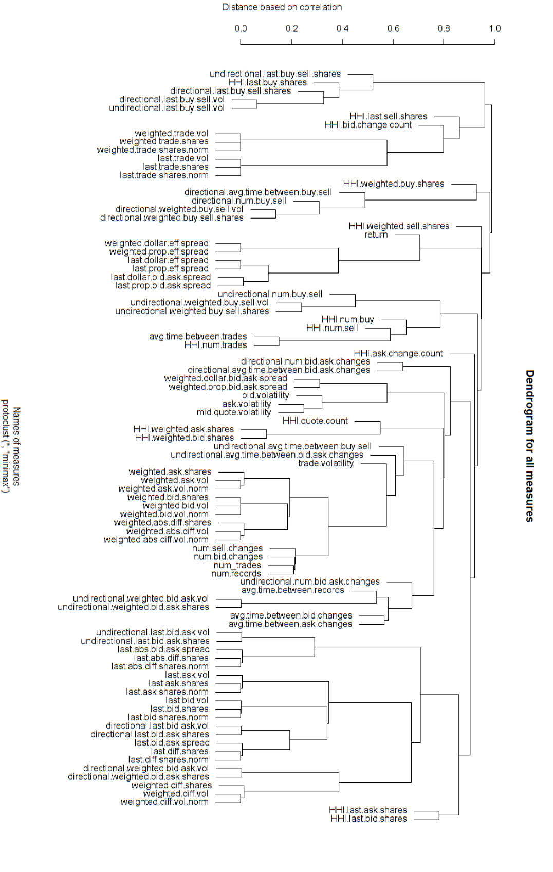
Figure 1: Dendrogram of all measures.

From the dendrogram, it is clear that the measures related to dollar volume always has a strong correlation with that related to the number of shares, since the price within a day does not change very much. Since we already have measures related to prices, here we should always use the measures related to the number of shares and remove redundant ones based on the dollar volume.

Also, the dollar effective spread always has strong correlation with proportional effective spread, since mid-quotes does not change much during one day. Therefore, in short horizon, we can abandon the dollar effective spread and only use the proportional effective spreads since they have normalization and will be comparable across the stocks.

Apart from the normalizing issue above, the measure normalizing by the average daily trading volume (or daily volatility) has correlation 1 with the original measure. So we only need one of each normalized / non-normalized pair. Since we want to make measures stable across all stocks, it is better to use the normalized ones. Therefore we should remove all non-normalized measures if there is an appropriate normalized one. The dendrogram after removing these redundant measures looks neater in Figure 2.

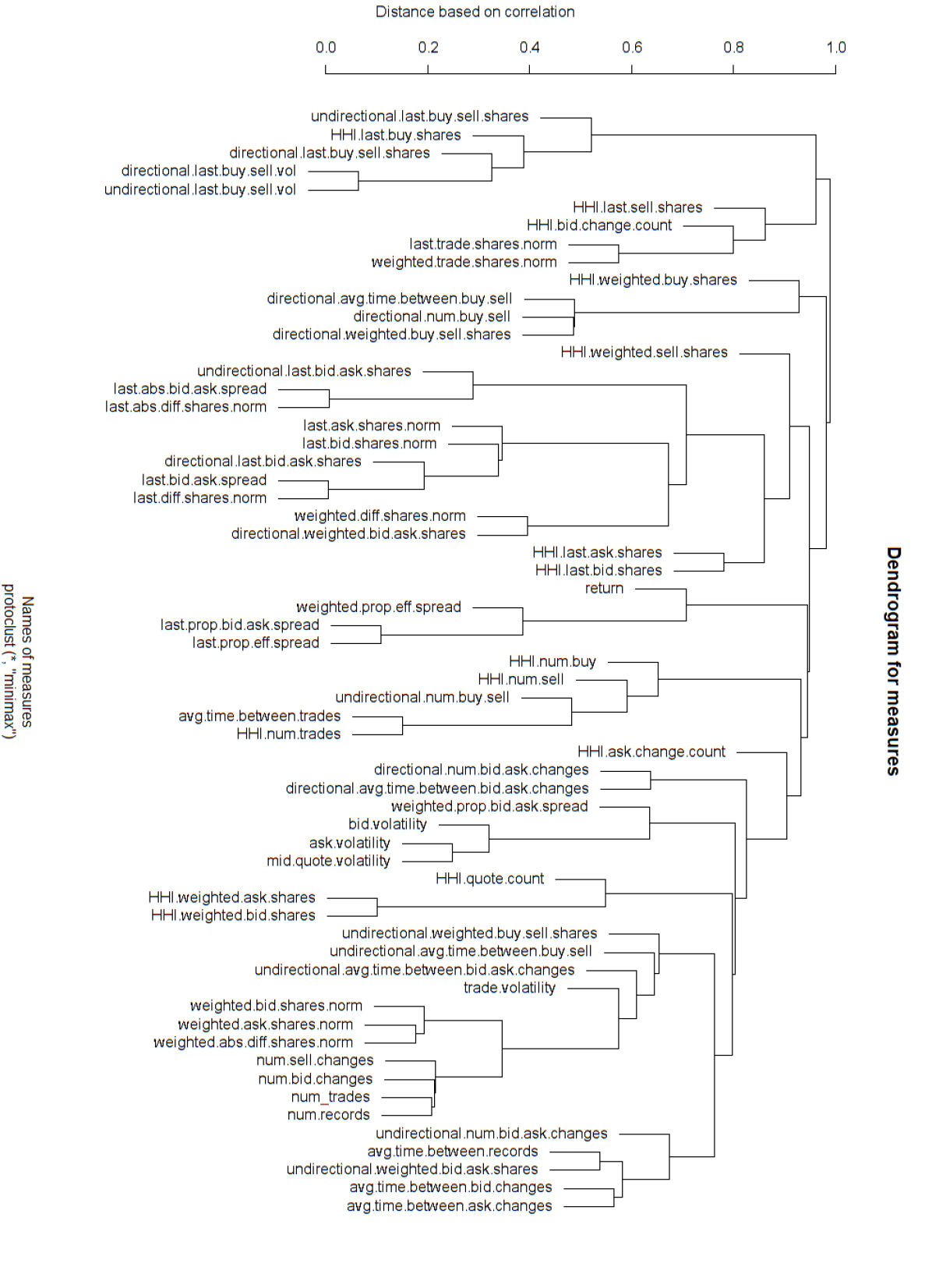
Figure 2: Dendrogram of measures after removing redundant ones.

There are no longer perfect correlated measures. However, there are still some interesting discoveries that is worthy for further study. For example, the last prevailing bid-ask spread (which is the last prevailing value of (ask price - bid price)) is strongly correlated with the last prevailing (ask shares - bid shares) / average daily trading shares. This suggests the relationship between quote prices and quote shares.

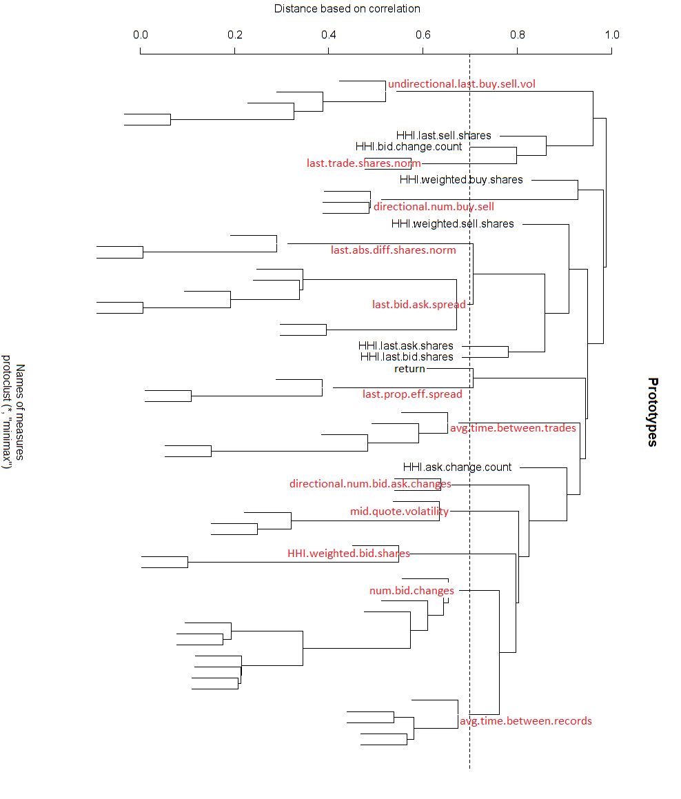
Figure 3: Prototypes selected.

Table 1: List of all selected measures.

No.	Names	Descriptions
1	return	Return
2	last.prop.eff.spread	The last prevailing proportional effective spread
3	mid.quote.volatility	Volatility based on mid-quote
4	num.bid.changes	The number of bid changes
5	avg.time.between.trades	Theaverage time between trades
6	last.trade.shares.norm	Thelast prevailing trade shares normalized by
		The average daily trading shares
7	directional.num.buy.sell	(buy - sell) / (buy + sell) where buy (sell) in
		the equation means the number of buy (sell)
		trades
8	undirectional.last.buy.sell.vol	$|$buy - sell$|$ / $|$buy + sell$|$ where buy (sell) in
		the equation means shares of buy (sell) trades
9	avg.time.between.records	The average time between quote records
10	last.bid.ask.spread	The last prevailing bid-ask spread
11	last.abs.diff.shares.norm	The last prevailing (ask shares - bid shares)
		normalized by the Average daily trading
		shares over the last month
12	directional.num.bid.ask.changes	(ask - bid) / (bid - ask) where ask (bid) in
		the equation means the number of ask (bid)
		changes
13	HHI.last.sell.shares	HHI of last sell prevailing shares
14	HHI.weighted.buy.shares	HHI of time-weighted buy shares
15	HHI.weighted.sell.shares	HHI of time-weighted sell shares
16	HHI.last.ask.shares	HHI of time-last ask shares
17	HHI.last.bid.shares	HHI of last prevailing bid shares
18	HHI.weighted.bid.shares	HHI of time-weighted bid shares
19	HHI.bid.change.count	HHI of count of bid changes
20	HHI.ask.change.count	HHI of count of ask changes

Finally, we use the prototype clustering to find good representatives (prototypes) of measures within each cluster, removing all redundant measures with correlation more than 0.3, in other word, distance less than 0.7). The dendrogram of the prototypes selected is shown in Figure 3. There are 20 measures (out of 91 original measures) selected. The list of selected measures is in Table 1.

5 Conclusion

Using the high-dimensional statistical methods, we find the 20 representative measures from all 91 candidates and meanwhile discover the relationship between measures. A clear clustering structure is given by the dendrogram. The clustering structure gives a clear interpretation of the representatives and relationship between different measures. Also, interesting phenomena can be found and can be studied within the clustering structure. The clustering structure provides the flexibility of modifying the number of features to use in future studies.

Future work can be done to use the selected measures to fit more exotic statistical models, such as time series models, machine learning models etc., to predict the stock returns.

References

- Bessembinder and Seguin (1993) Bessembinder, H. and Seguin, P. J. (1993). Price volatility, trading volume, and market depth: Evidence from futures markets. Journal of financial and Quantitative Analysis, 28(1):21–39.
- Bien and Tibshirani (2011) Bien, J. and Tibshirani, R. (2011). Hierarchical clustering with prototypes via minimax linkage. Journal of the American Statistical Association, 106(495):1075–1084.
- Bo et al. (2021) Bo, D., Hwangbo, H., Sharma, V., Arndt, C., and TerMaath, S. C. (2021). A subspace-based approach for dimensionality reduction and important variable selection. arXiv preprint arXiv:2106.01584.
- Chakrabarty et al. (2006) Chakrabarty, B., Li, B., Nguyen, V., and Van Ness, R. (2006). Trade classification algorithms for electronic communication networks. Journal of Banking and Finance, 31:3806–3821.
- Chan and Fong (2000) Chan, K. and Fong, W.-M. (2000). Trade size, order imbalance, and the volatility–volume relation. Journal of Financial Economics, 57(2):247–273.
- Chinco et al. (2017) Chinco, A. M., Clark-Joseph, A. D., and Ye, M. (2017). Sparse signals in the cross-section of returns. Technical report, National Bureau of Economic Research.
- Davis et al. (2021) Davis, D., Diaz, M., and Wang, K. (2021). Clustering a mixture of gaussians with unknown covariance. arXiv preprint arXiv:2110.01602.
- Du et al. (2020) Du, T., Zhang, Y., Shi, X., and Chen, S. (2020). Multiple slice k-space deep learning for magnetic resonance imaging reconstruction. In 2020 42nd Annual International Conference of the IEEE Engineering in Medicine & Biology Society (EMBC), pages 1564–1567. IEEE.
- Du et al. (2021) Du, W., Hyeon, E., Pei, H., Huang, Z., Cheong, Y., Zheng, S., and Galvanauskas, A. (2021). Improved machine learning algorithms for optimizing coherent pulse stacking amplification. In CLEO: Science and Innovations, pages JTh3A–1. Optical Society of America.
- Ellis et al. (2000) Ellis, K., Michaely, R., and O’Hara, M. (2000). The accuracy of trade classification rules: Evidence from nasdaq. Journal of Financial and Quantitative Analysis, 35(4):529–551.
- Glosten et al. (1993) Glosten, L. R., Jagannathan, R., and Runkle, D. E. (1993). On the relation between the expected value and the volatility of the nominal excess return on stocks. The Journal of Finance, 48(5):1779–1801.
- Herfindahl (1950) Herfindahl, O. C. (1950). Concentration in the steel industry. PhD thesis, Columbia University New York.
- Huang et al. (2020) Huang, X., Li, Z., Lu, J., Wang, S., Wei, H., and Chen, B. (2020). Time-series clustering for home dwell time during covid-19: what can we learn from it? ISPRS International Journal of Geo-Information, 9(11):675.
- Huang et al. (2021) Huang, X., Lu, J., Gao, S., Wang, S., Liu, Z., and Wei, H. (2021). Staying at home is a privilege: Evidence from fine-grained mobile phone location data in the united states during the covid-19 pandemic. Annals of the American Association of Geographers, 0(0):1–20.
- Jarrow et al. (2021) Jarrow, R. A., Murataj, R., Wells, M. T., and Zhu, L. (2021). The low-volatility anomaly and the adaptive multi-factor model. arXiv preprint arXiv:2003.08302.
- Jegadeesh and Titman (1993) Jegadeesh, N. and Titman, S. (1993). Returns to buying winners and selling losers: Implications for stock market efficiency. The Journal of Finance, 48(1):65–91.
- Jegadeesh et al. (1995) Jegadeesh, N., Titman, S., et al. (1995). Short-horizon return reversals and the bid-ask spread. Journal of Financial Intermediation, 4(2):116–132.
- Jie (2018) Jie, C. (2018). Decision Making Under Uncertainty: New Models and Applications. PhD thesis, University of Maryland, College Park.
- Jie et al. (2018) Jie, C., Prashanth, L., Fu, M., Marcus, S., and Szepesvári, C. (2018). Stochastic optimization in a cumulative prospect theory framework. IEEE Transactions on Automatic Control, 63(9):2867–2882.
- Kaufman and Rousseeuw (2009) Kaufman, L. and Rousseeuw, P. J. (2009). Finding Groups in Data: An Introduction to Cluster Analysis, volume 344. John Wiley & Sons.
- Kong et al. (2018) Kong, M., Salighehdar, A., and Bozdog, D. (2018). A study on brexit: Correlations and tail events distribution of liquidity measures. Journal of Management Science and Business Intelligence (JMSBI), 3(1).
- Lee and Ready (1991) Lee, C. and Ready, M. J. (1991). Inferring trade direction from intraday data. The Journal of Finance, 46(2):733–746.
- Li (2021) Li, J. (2021). Two ways towards combining sequential neural network and statistical methods to improve the prediction of time series. arXiv preprint arXiv:2110.00082.
- Li et al. (2021) Li, Y., Song, K., Sun, Y., and Zhu, L. (2021). Frequentnet: A novel interpretable deep learning model for image classification. arXiv preprint arXiv:2001.01034.
- Mao et al. (2020a) Mao, Y., Fu, Y., Zheng, W., Cheng, L., Liu, Q., and Tao, D. (2020a). Speculative container scheduling for deep learning applications in a kubernetes cluster. arXiv preprint arXiv:2010.11307.
- Mao et al. (2020b) Mao, Y., Yan, W., Song, Y., Zeng, Y., Chen, M., Cheng, L., and Liu, Q. (2020b). Differentiate quality of experience scheduling for deep learning applications with docker containers in the cloud. arXiv preprint arXiv:2010.12728.
- Roll (1984) Roll, R. (1984). A simple implicit measure of the effective bid-ask spread in an efficient market. The Journal of Finance, 39(4):1127–1139.
- Stein et al. (2021a) Stein, S. A., Baheri, B., Chen, D., Mao, Y., Guan, Q., Li, A., Fang, B., and Xu, S. (2021a). Qugan: A quantum state fidelity based generative adversarial network. In 2021 IEEE International Conference on Quantum Computing and Engineering (QCE), pages 71–81. IEEE.
- Stein et al. (2021b) Stein, S. A., Baheri, B., Chen, D., Mao, Y., Guan, Q., Li, A., Xu, S., and Ding, C. (2021b). Quclassi: A hybrid deep neural network architecture based on quantum state fidelity. arXiv preprint arXiv:2103.11307.
- Stein et al. (2020) Stein, S. A., Baheri, B., Tischio, R. M., Chen, Y., Mao, Y., Guan, Q., Li, A., and Fang, B. (2020). A hybrid system for learning classical data in quantum states. arXiv preprint arXiv:2012.00256.
- Wang et al. (2020) Wang, K., Yan, Y., and Diaz, M. (2020). Efficient clustering for stretched mixtures: Landscape and optimality. arXiv preprint arXiv:2003.09960.
- Zhang et al. (2021) Zhang, Y., Du, T., Sun, Y., Donohue, L., and Dai, R. (2021). Form 10-q itemization. arXiv preprint arXiv:2104.11783.
- Zhao et al. (2020) Zhao, Y., Landgrebe, E., Shekhtman, E., and Udell, M. (2020). Online missing value imputation and correlation change detection for mixed-type data via gaussian copula. arXiv preprint arXiv:2009.12326.
- Zhao et al. (2021) Zhao, Y., Matteson, D. S., Nebel, M. B., Mostofsky, S. H., and Risk, B. (2021). Group linear non-gaussian component analysis with applications to neuroimaging. arXiv preprint arXiv:2101.04809.
- Zhu (2020) Zhu, L. (2020). The Adaptive Multi-Factor Model and the Financial Market. eCommons.
- Zhu et al. (2020) Zhu, L., Basu, S., Jarrow, R. A., and Wells, M. T. (2020). High-dimensional estimation, basis assets, and the adaptive multi-factor model. The Quarterly Journal of Finance, 10(04):2050017.
- Zhu et al. (2021a) Zhu, L., Jarrow, R. A., and Wells, M. T. (2021a). Time-invariance coefficients tests with the adaptive multi-factor model. The Quarterly Journal of Finance, 11(04):2150019.
- Zhu et al. (2021b) Zhu, L., Wu, H., and Wells, M. T. (2021b). A news-based machine learning model for adaptive asset pricing. arXiv preprint arXiv:2106.07103.