Near-optimal inference in adaptive linear regression

Abstract

When data is collected in an adaptive manner, even simple methods like ordinary least squares can exhibit non-normal asymptotic behavior. As an undesirable consequence, hypothesis tests and confidence intervals based on asymptotic normality can lead to erroneous results. We propose a family of online debiasing estimators to correct these distributional anomalies in least squares estimation. Our proposed methods take advantage of the covariance structure present in the dataset and provide sharper estimates in directions for which more information has accrued. We establish an asymptotic normality property for our proposed online debiasing estimators under mild conditions on the data collection process and provide asymptotically exact confidence intervals. We additionally prove a minimax lower bound for the adaptive linear regression problem, thereby providing a baseline by which to compare estimators. There are various conditions under which our proposed estimators achieve the minimax lower bound. We demonstrate the usefulness of our theory via applications to multi-armed bandit, autoregressive time series estimation, and active learning with exploration.

, ,
, , and

1 Introduction

Consider a prediction problem in which we observe $n$ datapoints of the form $(\mathbf{x}_{i},y_{i})\in\bf{R}^{d}\times\bf{R}$ with covariate vector $\mathbf{x}_{i}$ and response $y_{i}$ linked via the linear model

$$y_{i}=\big{\langle}\mathbf{x}_{i},{\boldsymbol{\theta}^{*}}\big{\rangle}+\mathbf{\epsilon}_{i}\quad\mbox{for $i=1,\ldots,n$.}$$ (1)

Here the vector ${\boldsymbol{\theta}^{*}}\in\bf{R}^{d}$ is an unknown parameter of interest, and $\mathbf{\epsilon}_{i}$ is additive noise. When the datapoints are generated via some i.i.d. sampling process, this model, and in particular the behavior of the ordinary least squares (OLS) estimate $\widehat{\boldsymbol{\theta}}_{\scriptscriptstyle{\operatorname{LS}}}$, is very well-understood. The focus of this paper is the more challenging setting in which the covariate vectors $\{\mathbf{x}_{i}\}_{i=1}^{n}$ have been adaptively collected, meaning that the choice of $\mathbf{x}_{i}$ can depend on the entire set of previous observations $\{\mathbf{x}_{j},y_{j}\}_{j=1}^{i-1}$.

More precisely, given a filtration $\{\mathcal{F}_{i}\}_{i=1}^{n}$, assume that $\mathbf{x}_{i}$ is $\mathcal{F}_{i-1}$-measurable and that the additive error $\{\mathbf{\epsilon}_{i}\}_{i=1}^{n}$ is a martingale difference sequence with respect to $\{\mathcal{F}_{i}\}_{i=1}^{n}$, with

$$\operatorname{\mathbb{E}}[\mathbf{\epsilon}_{i}\mid\mathcal{F}_{i-1}]=0,\quad\mbox{and}\quad\operatorname{\mathbb{E}}[\mathbf{\epsilon}_{i}^{2}\lvert\mathcal{F}_{i-1}]=\sigma^{2},$$ (2)

for some non-random scalar $\sigma^{2}>0$. We refer to the combination of the linear observation model (1) with such (potentially) adaptive collection procedures as the adaptive linear regression model. Instances of adaptive linear regression arise in a variety of applications, including multi-armed bandits [20], active learning [9], times series modeling [4], stochastic control [1], and adaptive stochastic approximation schemes [18, 6].

Let us discuss some known results for the OLS estimate $\widehat{\boldsymbol{\theta}}_{\scriptscriptstyle{\operatorname{LS}}}$. The estimate can be expanded in the form

$$\widehat{\boldsymbol{\theta}}_{\scriptscriptstyle{\operatorname{LS}}}=\mathbf{S}_{n}^{-1}\mathbf{X}_{n}^{\top}y_{n}={\boldsymbol{\theta}^{*}}+\mathbf{S}_{n}^{-1}\sum_{i=11}^{n}\mathbf{x}_{i}\mathbf{\epsilon}_{i},\qquad\text{where}\quad\mathbf{S}_{n}:\,=\sum_{i=1}^{n}\mathbf{x}_{i}\mathbf{x}_{i}^{\top}.$$ (3)

This decomposition reveals that the statistical properties of the OLS estimate depend on the martingale transform $\sum_{i=1}^{n}\mathbf{x}_{i}\mathbf{\epsilon}_{i}$, along with the random matrix $\mathbf{S}_{n}$. There is a lengthy literature on conditions under which the OLS estimate is consistent [18, 1, 4, 10, 16, 17]. Notably, Lai and Wei [18, Thm. 1] show that the OLS estimate is strongly consistent, meaning that $\widehat{\boldsymbol{\theta}}_{\scriptscriptstyle{\operatorname{LS}}}\stackrel{{\scriptstyle{\operatorname{a.s.}}}}{{\longrightarrow}}{\boldsymbol{\theta}^{*}}$, whenever

$$\lambda_{\min}(\mathbf{S}_{n})\stackrel{{\scriptstyle{\operatorname{a.s.}}}}{{\longrightarrow}}\infty\quad\text{and}\quad\frac{\log\lambda_{\max}(\mathbf{S}_{n})}{\lambda_{\min}(\mathbf{S}_{n})}\stackrel{{\scriptstyle{\operatorname{a.s.}}}}{{\longrightarrow}}0.$$ (4)

Arguably, these conditions for consistency are quite mild. In contrast, Lai and Wei [18, Theorem 3] also show that asymptotic normality of the least squares estimator in the adaptive linear regression model holds under a stability condition that is substantially more restrictive—namely, the existence of a sequence $\{\mathbf{B}_{n}\}_{n\geq 1}$ of non-random strictly positive definite matrices such that

$$\mathbf{B}_{n}^{-1}\mathbf{S}_{n}\stackrel{{\scriptstyle{\operatorname{p}}}}{{\longrightarrow}}\mathbf{I}.$$ (5)

Moreover, Lai and Wei [18, Example 3] demonstrate through the example of a unit root autoregressive model that the OLS estimator fails to be asymptotically normal in absence of the stability property (5). In such cases, confidence intervals and other forms of inference performed using Gaussian limit theory are no longer valid.

Contributions

In this paper, we propose and analyze a new family of estimators for the parameter vector ${\boldsymbol{\theta}^{*}}$ (or linear functionals thereof) based on online debiasing techniques. We show that, under mild conditions, our proposed estimators are both asymptotically unbiased and asymptotically normal. The underlying assumptions are less stringent than the stability condition (5) and are satisfied by a large class of models for data generation and protocols for choosing covariate vectors. We provide a detailed discussion of three such example classes in Section 4. By deriving minimax lower bounds on the performance of any estimator, we show that our estimators are minimax optimal. We also show that the asymptotic performance of these estimators are near-optimal in an instance dependent sense, in that they match the performance of the best problem-specific behavior up to a logarithmic factor.

Related work

The broader literature on bandit algorithms and experimentation focuses mostly on a single statistical objective, with standard examples being minimizing regret or selecting an optimal arm with high probability. In the papers [29, 26], the authors empirically observed that bandit algorithms induce bias, which can be problematic for ex-post inference. Later works [21, 22, 23] characterize the sign and bound the magnitude of this bias. In the paper [11], the authors develop estimators that use propensity scores for the multi-armed bandit setting, a special case of the stochastic regression model (1) in which the covariate vectors $\mathbf{x}_{i}$ are restricted to standard basis vectors. However, it is not clear how to extend this approach to general designs. Also in the bandit setting, Zhang et al. [30] develop a least squares estimator that exploits an assumed batch structure, meaning that only a fixed, finite number of adaptive decisions are made. This approach, however, does not apply to more general schemes that make adaptive decisions at each round. Recently, Zhang et al. [31] proposed a weighted M-estimator for contextual bandit problems where the bandit algorithm is known. It is also not clear how to generalize this approach to a more general data collection scheme or to the case when the data collection algorithm is not completely known.

There is also a parallel line of work that exploits concentration of measure results (e.g., see the papers [3, 27]) to develop confidence regions that are valid uniformly in time. This approach has its roots in the bandits literature [2, 13] and has been refined in more recent work [12, 14]. An advantage of this approach is that it yields bounds that are uniform in time. On the flip side, it requires very strong exponential tail conditions on the error sequence in contrast to the relatively mild moment conditions that we impose. Overall, we view this line of work as being complementary to our goal of developing corrected estimators that obey asymptotic normality.

This paper builds upon and extends past work, due to a subset of the current authors [6, 5], using online debiasing techniques. In 2, we prove a lower bound that shows how the matrix sequence $\mathbf{S}_{n}^{-1}$ controls the fundamental difficulty of the problem, and this lower bound also motivates the particular form of debiasing proposed in this paper. The construction used in past work [6, 5] is based on a non-adaptive upper bound of the form $\lambda_{*}\mathbf{I}$, where the scalar $\lambda_{*}$ is chosen to be much larger than $\lambda_{\max}(\mathbf{S}_{n}^{-1})$ with high probability. By sharp contrast, our analysis instead makes use of an adaptive upper bound that simultaneously respects the structure of $\mathbf{S}_{n}^{-1}$ and leads to a stable martingale transform; this particular construction and our analysis thereof allows us to obtain sharper guarantees than past work [6, 5].

Notation

Let us summarize some notation used throughout the remainder of the paper. For a positive integer $n$, we make use of the convenient shorthand $[n]:\,=\{1,2,\ldots,n\}$. We use $\mathbf{e}_{j}$ to denote the $j$th standard basis vector in $\bf{R}^{d}$. For a matrix $\mathbf{M}$, we use the notation $|\!|\!|\mathbf{M}|\!|\!|_{{\scriptsize{\operatorname{op}}}}$ and $|\!|\!|\mathbf{M}|\!|\!|_{{\scriptsize{\operatorname{F}}}}$ to denote the operator norm (maximum singular value) and the Frobenius norm of the matrix $\mathbf{M}$, respectively; similarly, we use the notation $\|\mathbf{M}\|_{\scriptsize{\operatorname{max}}}$ to denote the maximum entry in absolute value. For a square matrix $\mathbf{S}$, the quantities $\lambda_{\max}(\mathbf{S})$ and $\lambda_{\min}(\mathbf{S})$ respectively denote the maximum and minimum eigenvalue of the matrix $\mathbf{S}$. The quantity $\operatorname{trace}(\mathbf{S})$ denotes the sum of diagonal entries of the square matrix $\mathbf{S}$. For a pair of squares matrices $(\mathbf{A},\mathbf{B})$ of compatible dimensions, we use the notation $\mathbf{A}\succcurlyeq\mathbf{B}$ to indicate that the difference matrix $\mathbf{A}-\mathbf{B}$ is positive semidefinite; we use the notation $\mathbf{A}\succ\mathbf{B}$ when the difference matrix $\mathbf{A}-\mathbf{B}$ is positive definite. The relations $\mathbf{A}\preccurlyeq\mathbf{B}$ and $\mathbf{A}\prec\mathbf{B}$ are defined analogously. For a symmetric positive semidefinite matrix $\mathbf{S}$, we use $\mathbf{S}^{\frac{1}{2}}$ to denote its symmetric matrix square root.

For a sequence of random variables $\{Z_{n}\}_{n\geq 1}$ and a random variable $Z$, we write $Z_{n}\stackrel{{\scriptstyle{\operatorname{p}}}}{{\longrightarrow}}Z$ to mean that the sequence of random variables $\{Z_{n}\}_{n\geq 1}$ converges to $Z$ in probability; the notation $Z_{n}\stackrel{{\scriptstyle{\operatorname{d}}}}{{\longrightarrow}}Z$ indicates convergence in distribution. For a sequence of real-valued random variables $\{Z_{n}\}_{n\geq 1}$ and a sequence of non-zero real numbers $\{a_{n}\}_{n\geq 1}$, we write $Z_{n}=o_{p}(a_{n})$ to mean that the ratio $\tfrac{Z_{n}}{a_{n}}\stackrel{{\scriptstyle{\operatorname{p}}}}{{\longrightarrow}}0$. We write $Z_{n}=O_{p}(a_{n})$ to mean that the ratio $Z_{n}/a_{n}$ is stochastically bounded. More precisely, for every scalar $\epsilon>0$, there exits a positive real number $C_{\epsilon}$ such that $\sup\limits_{n\geq 1}\,\mathbb{P}[Z_{n}/a_{n}>C_{\epsilon}]<\epsilon$.

2 From ordinary least squares to online debiasing

In this section, we begin by motivating the work by discussing how classical theory about ordinary least squares estimate can break down when data is collected in an adaptive manner. We then introduce an online debiasing approach to computing alternative estimates.

2.1 Breakdown of the ordinary least squares estimator

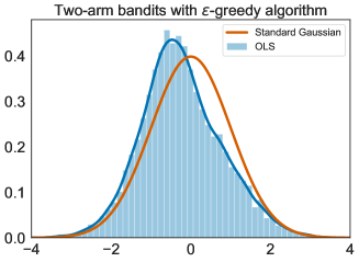
(a) Distribution of $\frac{{\widehat{\boldsymbol{\theta}}}_{2}-\theta_{2}^{*}}{\sqrt{(\mathbf{S}_{n}^{-1})_{22}}}$

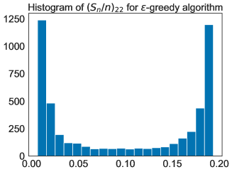
(b) Distribution of $\left(\mathbf{S}_{n}/n\right)_{22}$

Figure 1: Quantitative behavior of the first coordinate ${\widehat{\boldsymbol{\theta}}}_{1}$ of the ordinary least squares estimator $\widehat{\boldsymbol{\theta}}_{\scriptscriptstyle{\operatorname{LS}}}:=({\widehat{\boldsymbol{\theta}}}_{1},{\widehat{\boldsymbol{\theta}}}_{2})$ on a dataset drawn from the $\varepsilon$-greedy two-armed bandit model of Section 2.1. The results are obtained with a dataset of size $n=1000$ and $5000$ independent replications. (a) The distribution of the rescaled difference $\frac{{\widehat{\boldsymbol{\theta}}}_{2}-\theta_{2}^{*}}{\sqrt{(\mathbf{S}_{n}^{-1})_{22}}}$ is far from standard Gaussian. (b) The bimodal distribution of $\left(\mathbf{S}_{n}/n\right)_{22}$ suggests that the scaled covariance matrix $\mathbf{S}_{n}/n$ does not converge to a deterministic matrix.

Let us begin by considering the behavior of the OLS estimator $\widehat{\boldsymbol{\theta}}_{\scriptscriptstyle{\operatorname{LS}}}$ from equation (3). When the covariates $\{\mathbf{x}_{i}\}_{i\geq 1}$ are either fixed or independently sampled from a fixed distribution, it has several optimality properties. Accordingly, it is natural to ask what the performance of the OLS estimator is when the covariates $\{\mathbf{x}_{i}\}$ are drawn in an adaptive manner.

In order to fix ideas, let us consider a two-armed bandit problem [20], a special case of the linear regression model (1) with each $\mathbf{x}_{i}$ chosen to be either $(1,0)^{\top}$ or $(0,1)^{\top}$ based on the prior data $\{\mathbf{x}_{j},y_{j}\mid j\leq i-1\}$. In order to generate the covariates $\{\mathbf{x}_{i}\}_{i=1}^{n}$, suppose that we apply the $\varepsilon$-greedy selection algorithm, a popular choice for tackling bandit problems [20].

A simple simulation reveals some interesting phenomena. We generated linear regression data using $\varepsilon$-greedy selection algorithm with the choices $\varepsilon=0.1$, ${\boldsymbol{\theta}^{*}}=(0.3,0.3)^{\top}$, and noise variables $\mathbf{\epsilon}_{i}\stackrel{{\scriptstyle i.i.d.}}{{\sim}}\mathcal{N}(0,1)$. Let ${\widehat{\boldsymbol{\theta}}}_{2}$ denote the first coordinate of the OLS estimator fit to the bandit data. Figure 1(a) demonstrates that the distribution of ${\widehat{\boldsymbol{\theta}}}_{2}$, even after proper re-centering and scaling, does not converge to a standard normal distribution. As an undesirable consequence, the confidence intervals for $\theta^{*}_{2}$, usually constructed using the quantiles of a standard normal random variable, are not valid.

Let us try to understand why the OLS estimate fails to be asymptotically normal. Figure 1(b) plots a histogram of the $(2,2)$ entry of the scaled sample covariance matrix $\mathbf{S}_{n}/n$. The bimodal behavior suggests that $\mathbf{S}_{n}/n$ fails to converge to a non-random matrix $\mathbf{B}$ and indicates that the stability condition (5) is not satisfied. Indeed, in a recent paper [30], the authors show that when $\theta_{1}^{*}=\theta_{2}^{*}$ as in our example, the OLS estimator, after proper centering and scaling, converges to a distribution which is not a standard Gaussian distribution.

It turns out that this distributional anomaly of the OLS estimator is neither specific to the two-armed bandit problem [20] nor to the $\varepsilon$-greedy algorithm used to simulate the data for Figure 1. The same phenomenon was documented in the time-series and forecasting literature half a century ago, dating back to the works of White [28], Dickey and Fuller [7] and Lai and Wei [18]. More recent work [6, 30] has highlighted that a similar phenomenon commonly occurs in multi-armed bandit problems when using popular selection algorithms, including Thompson sampling and the upper confidence bound (UCB) algorithm [20].

In Section 2.2, we rectify the distributional anomaly of the OLS estimator by proposing an estimator based on the online debiasing principles of Deshpande et al. [6] and show that our online debiasing estimator exhibits asymptotic normality even in the absence of the stability condition (5). In Section 4, we demonstrate the usefulness of our theory via applications to the multi-armed bandit problems, autoregressive time series, and active learning problems with exploration.

2.2 Online debiasing estimator

In this section, we propose and analyze an estimator based on an online debiasing technique motivated by the work of Deshpande et al. [6]. At a high-level, the estimator involves a specific perturbation of the ordinary least squares estimator $\widehat{\boldsymbol{\theta}}_{\scriptscriptstyle{\operatorname{LS}}}$. This perturbation is constructed via a linear combination of the prediction errors $\{y_{i}-\big{\langle}\mathbf{x}_{i},\widehat{\boldsymbol{\theta}}_{\scriptscriptstyle{\operatorname{LS}}}\big{\rangle}\}_{i=1}^{n}$ along with a carefully chosen sequence of weight vectors $\{\mathbf{w}_{i}\}_{i=1}^{n}$. The key property ensured by the construction is that the weight vector $\mathbf{w}_{i}$ is $\mathcal{F}_{i-1}$ measurable for each $i\in[n]$.

Concretely, for weight vectors $\{\mathbf{w}_{i}\}_{i=1}^{n}$, we compute the online debiasing estimate

$$\widehat{\boldsymbol{\theta}}_{\scriptscriptstyle{\operatorname{OD}}} :\,=\widehat{\boldsymbol{\theta}}_{\scriptscriptstyle{\operatorname{LS}}}+\mathbf{S}_{n}^{-\frac{1}{2}}\sum_{i=1}^{n}\mathbf{w}_{i}(y_{i}-\big{\langle}\mathbf{x}_{i},\widehat{\boldsymbol{\theta}}_{\scriptscriptstyle{\operatorname{LS}}}\big{\rangle}).$$ (6)

Here the reader should recall our earlier definition $\mathbf{S}_{n}:\,=\sum_{i=1}^{n}\mathbf{x}_{i}\mathbf{x}_{i}^{\top}$, and throughout, we assume that the sample covariance $\mathbf{S}_{n}$ is invertible. The matrix $\mathbf{S}_{n}^{-\frac{1}{2}}$ denotes a symmetric matrix square root of $\mathbf{S}_{n}^{-1}$.

Of course, there is an infinite family of estimators of the form (6), and the key question is how to define the weight vectors. In this paper, we propose an estimator in which the sequence $\{\mathbf{w}_{i}\}_{i=1}^{n}$ is obtained by solving an optimization problem that takes three inputs:

1. the original data $\{(\mathbf{x}_{i},y_{i})\}_{i=1}^{n}$,

2. a non-random scalar $\gamma_{n}\in(0,1]$, and

3. a sequence of symmetric positive semidefinite matrices $\{\mathbf{\Gamma}_{i}\}_{i=1}^{n}$ such that $\mathbf{\Gamma}_{i}\in\mathcal{F}_{i-1}$ for each $i\in[n]:\,=\{1,\ldots,n\}$.

In order to simplify notation, we adopt the shorthand $\mathbf{z}_{i}:\,=\mathbf{\Gamma}_{i}^{-\frac{1}{2}}\mathbf{x}_{i}$. Moreover, for each index $i\in[n]$, we define the matrices

$$\mathbf{Z}_{i}^{\top}:\,=\begin{bmatrix}\mathbf{z}_{1}&\mathbf{z}_{2}&\cdots&\mathbf{z}_{i}\end{bmatrix},\quad\mbox{and}\quad\mathbf{W}_{i}:\,=\begin{bmatrix}\mathbf{w}_{1}&\mathbf{w}_{2}&\cdots&\mathbf{w}_{i}\end{bmatrix}$$

We also define $\mathbf{W}_{0}=0$ and $\mathbf{Z}_{0}=0$. With these definitions, the vectors $\{\mathbf{w}_{i}\}_{i=1}^{n}$ are obtained recursively by solving the following convex program

$$\mathbf{w}_{i} :\,=\arg\min_{\mathbf{w}\in\bf{R}^{d}}\left\{|\!|\!|\mathbf{I}-\mathbf{W}_{i-1}\mathbf{Z}_{i-1}-\mathbf{w}\mathbf{z}_{i}^{\top}|\!|\!|_{{\scriptsize{\operatorname{F}}}}^{2}+\frac{\gamma_{n}}{2}\|\mathbf{w}\|_{2}^{2}\right\}\quad\mbox{for $i=1,2,\ldots,n$.}$$ (7a)

Conveniently, this optimization problem has the explicit solution

$$\mathbf{w}_{i} =\frac{(\mathbf{I}-\mathbf{W}_{i-1}\mathbf{Z}_{i-1})\mathbf{z}_{i}}{(\gamma_{n}/2)+\|\mathbf{z}_{i}\|_{2}^{2}}.$$ (7b)

3 Main results

Having motivated and introduced the online debiasing approach, we now turn to some theoretical guarantees that can be given for these methods. We begin in Section 3.1 by providing sufficient conditions for the online debiasing estimator of Section 2.2 to exhibit asymptotically Gaussian behavior (1). In Section 3.2, we provide an asymptotically exact confidence region for ${\boldsymbol{\theta}^{*}}$ as well as an asymptotically exact confidence interval (Proposition 1) for ${\mathbf{v}}^{\top}{\boldsymbol{\theta}^{*}}$, where ${\mathbf{v}}$ is an arbitrary fixed direction ${\mathbf{v}}\in\bf{R}^{d}$. In Section 3.3—in particular, see 2—we complement these results by providing minimax lower bounds on a family of Mahalanobis errors and the length of confidence intervals. These lower bounds apply to any estimator for the stochastic regression model which does not know the true value of the target parameter ${\boldsymbol{\theta}^{*}}$ but may have the full knowledge of how the data was collected. Finally, in Section 3.4 we provide general strategies which can be used to verify the conditions of 1. All of our asymptotic statements assume that the dimension $d$ is fixed (constant) while the sample size $n$ grows.

3.1 Asymptotic normality guarantees

The main result of this section is an asymptotic normality guarantee for the proposed estimator (6), where the weight vectors are defined via the recursion (7).

We begin by stating our assumptions and providing some intuition about their role in the theorem.

Assumption A

1. There are positive scalars $\sigma$ and $\Delta$ such that the noise sequence $\{\mathbf{\epsilon}_{i}\}_{i=1}^{n}$ satisfies the conditions $\operatorname{\mathbb{E}}[\mathbf{\epsilon}_{i}\mid\mathcal{F}_{i-1}]=0$ and $\operatorname{\mathbb{E}}[\mathbf{\epsilon}_{i}^{2}\mid\mathcal{F}_{i-1}]=\sigma^{2}$ for all $i\in[n]$ and moreover

   $$\max_{i\in[n]}\;\operatorname{\mathbb{E}}[\mathbf{\epsilon}_{i}^{2+\Delta}\mid\mathcal{F}_{i-1}]<\infty.$$

2. The sequence of matrices $\{\mathbf{S}_{n}\}_{n\geq 1}$ satisfy the conditions $\lambda_{\min}(\mathbf{S}_{n})\stackrel{{\scriptstyle{\operatorname{a.s.}}}}{{\longrightarrow}}\infty$ and $\frac{\log\lambda_{\max}(\mathbf{S}_{n})}{\lambda_{\min}(\mathbf{S}_{n})}\stackrel{{\scriptstyle{\operatorname{a.s.}}}}{{\longrightarrow}}0$.

3. For each $n$, the scalar $\gamma_{n}>0$ and positive semidefinite matrices $\{\mathbf{\Gamma}_{i}\}_{i=1}^{n}$ with $\mathbf{\Gamma}_{i}\in\mathcal{F}_{i-1}$ are chosen such that:

   $$\max\limits_{i\in[n]}\;\;\left\{\frac{1}{\gamma_{n}}\big{\langle}\mathbf{x}_{i},\mathbf{\Gamma}_{i}^{-1}\mathbf{x}_{i}\big{\rangle}\right\} \stackrel{{\scriptstyle{\operatorname{p}}}}{{\longrightarrow}}0,$$ (a) Asymptotic negligibility:

   $$\sqrt{\gamma_{n}\log\lambda_{\max}(\mathbf{S}_{n})}\cdot|\!|\!|\mathbf{I}-\mathbf{W}_{n}\mathbf{X}_{n}\mathbf{S}_{n}^{-\frac{1}{2}}|\!|\!|_{{\scriptsize{\operatorname{op}}}} \stackrel{{\scriptstyle{\operatorname{p}}}}{{\longrightarrow}}0,\quad\mbox{and}$$ (b) Vanishing bias:

   $$|\!|\!|\mathbf{I}-\sum_{i=1}^{n}\mathbf{w}_{i}\mathbf{x}_{i}^{\top}\mathbf{\Gamma}_{i}^{-\frac{1}{2}}|\!|\!|_{{\scriptsize{\operatorname{op}}}} \stackrel{{\scriptstyle{\operatorname{p}}}}{{\longrightarrow}}0.$$ (c) Variance stability:

Let us provide some intuition for the role of each of these assumptions in the theorem. First, Assumption (A1) is quite simple: it imposes relatively mild moment conditions on the noise variables. Second, as discussed in the introduction, Assumption (A2) is standard in guaranteeing the consistency of the least squares estimate. Both Assumptions (A1) and (A2) are viewed as mild conditions in the stochastic linear regression literature and are satisfied by many practical models including those studied in the papers [16, 18, 15, 6]. Note that Assumptions (A1) and (A2) concern the regression model itself as opposed to the method: in particular, they do not depend on the algorithm parameters $\gamma_{n}$ and $\{\mathbf{\Gamma}_{i}\}_{i=1}^{n}$.

The more subtle requirements for our theorem to apply, which do depend on the algorithm parameters, are stated in Assumption (A3). We discuss the technical role of these conditions in the comments after 1, to be stated momentarily. In Section 3.4 to follow, we provide concrete choices of the algorithm parameters $\gamma_{n}$ and $\{\mathbf{\Gamma}_{i}\}_{i=1}^{n}$ that ensure that Assumption (A3) holds.

Finally, it should be noted that Assumption (A3) is weaker than the stability condition (5). Indeed, if the stability condition (5) and the growth condition (A2) are satisfied, then we may take $\gamma_{n}=1$, $\mathbf{\Gamma}_{i}=\mathbf{B}_{n}$ and $\mathbf{w}_{i}=\mathbf{B}_{n}^{-\frac{1}{2}}\mathbf{x}_{i}$. With these choices, the conditions (A3) are automatically satisfied; moreover, in this particular case, the online debiased estimator reduces to ordinary least squares; see 3 for details.

With these preliminaries in place, we are now equipped to state our main theorem on the online debiasing estimator $\widehat{\boldsymbol{\theta}}_{\scriptscriptstyle{\operatorname{OD}}}$:

Theorem 1.

Let $\widehat{\sigma}^{2}$ be any consistent estimator of $\sigma^{2}$. Then under Assumptions (A1)–(A3), we have

$$\sqrt{\frac{\gamma_{n}}{\widehat{\sigma}^{2}}}\cdot\mathbf{S}_{n}^{\frac{1}{2}}(\widehat{\boldsymbol{\theta}}_{\scriptscriptstyle{\operatorname{OD}}}-{\boldsymbol{\theta}^{*}})\stackrel{{\scriptstyle{\operatorname{d}}}}{{\longrightarrow}}\mathcal{N}(0,\mathbf{I}).$$ (9)

We prove this theorem in Section 5.1.

A few comments on this theorem are in order. First, needing a consistent estimate of the error variance $\sigma^{2}$ is a mild requirement. For instance, under our conditions, the estimator

$$\widehat{\sigma}^{2}=\frac{1}{n}\sum_{i=1}^{n}\left(y_{i}-\mathbf{x}_{i}^{\top}\widehat{\boldsymbol{\theta}}_{\scriptscriptstyle{\operatorname{LS}}}\right)^{2}$$

is strongly consistent; see Lemma 3 in the paper [18] for details.

A second important fact is that Assumption (A3) is considerably weaker than the stability condition (5) required for asymptotic normality of the OLS estimate. To reinforce this point, Section 4 provides a detailed discussion of three classes of problems for which OLS fails to be asymptotically normal but the guarantee (9) still holds for the online debiasing estimator.

Of all the conditions of 1, verifying the variance stability condition in part (c) of Assumption (A3) is the most challenging, and our arguments for doing so vary from problem to problem. In Corollaries 1 and 2, we verify the variance stability condition for multi-armed bandit problems and autoregressive time series models, respectively. In Corollary 3, we verify this condition for a large class of problems satisfying a sufficient exploration condition. In Section 3.4 to follow, we argue that when $\lambda_{\min}(\mathbf{S}_{n})\geq\log^{2}(n)$, we can always find choices of the tuning parameters $\gamma_{n}$ and $\{\Gamma_{i}\}$ such that Assumption (A3) is satisfied. Additionally, in absence of such lower bound on $\lambda_{\min}(\mathbf{S}_{n})$, we propose a data-augmentation strategy that gets rids of this growth condition at the cost of collecting additional $\log^{2}(n)$ many data-points.

Let us now discuss how Assumption (A3) enters the proof of Theorem 1. Our argument is based on the decomposition

$$\sqrt{\gamma_{n}}\cdot\mathbf{S}_{n}^{\frac{1}{2}}(\widehat{\boldsymbol{\theta}}_{\scriptscriptstyle{\operatorname{OD}}}-{\boldsymbol{\theta}^{*}}) =\mathbf{b}_{n}+\mathbf{v}_{n},\quad\mbox{where}$$ (10a)

$$\mathbf{b}_{n} :\,=\sqrt{\gamma_{n}}\cdot\left(\mathbf{I}-\mathbf{W}_{n}\mathbf{X}_{n}\mathbf{S}_{n}^{-\frac{1}{2}}\right)(\widehat{\boldsymbol{\theta}}_{\scriptscriptstyle{\operatorname{LS}}}-{\boldsymbol{\theta}^{*}})\quad\mbox{and}$$ (10b)

$$\mathbf{v}_{n} :\,=\sqrt{\gamma_{n}}\cdot\sum_{i=1}^{n}\mathbf{w}_{i}\mathbf{\epsilon}_{i}.$$ (10c)

By construction (and suggested by our notation), the term $\mathbf{b}_{n}$ corresponds to the bias in our estimate, a quantity that must be shown to vanish in order for our claim to hold. In order to do so, we first derive an upper bound on the norm $\|\mathbf{b}_{n}\|_{2}$. The “vanishing bias” condition stated in Assumption (A3)(b) enters in showing that, via our choices of the tuning parameters $\gamma_{n}$ and $\{\mathbf{\Gamma}_{i}\}_{i=1}^{n}$, this upper bound converges to zero in probability.

The random vector $\mathbf{v}_{n}$ defines a zero-mean martingale, and our proof controls its behavior via a standard martingale central limit theorem. Doing so requires a Lindeberg type condition on the weight vectors $\{\mathbf{w}_{i}\}_{i=1}^{n}$, as given in part (a) of Assumption (A3). Moreover, it requires that the conditional covariance of the martingale behave suitably, in which context part (c) of Assumption (A3) enters.

3.2 Obtaining confidence regions and intervals

In this section, we use the online debiasing procedure to obtain asymptotically exact confidence regions and intervals.

3.2.1 Confidence region for ${\boldsymbol{\theta}^{*}}$

First, for some user-defined level $\alpha\in(0,1)$, consider the problem of finding a confidence region for ${\boldsymbol{\theta}^{*}}$—that is, a (random) set $\mathbf{A}_{1-\alpha}$ that contains ${\boldsymbol{\theta}^{*}}$ with probability at least $1-\alpha$. We would like a set that is as small as possible, asymptotically exact in the sense that its coverage converges to $1-\alpha$.

Theorem 1 allows us to construct such a set in the following straightforward way. For any $\alpha\in(0,1)$, consider the subset of $\bf{R}^{d}$ given by

$$\mathbf{A}_{1-\alpha}=\left\{\mathbf{\theta}\in\bf{R}^{d}\mid\frac{\gamma_{n}}{{\widehat{\sigma}}^{2}}\cdot(\widehat{\boldsymbol{\theta}}_{\scriptscriptstyle{\operatorname{OD}}}-\theta)^{\top}\mathbf{S}_{n}(\widehat{\boldsymbol{\theta}}_{\scriptscriptstyle{\operatorname{OD}}}-\theta)\leq\chi^{2}_{d,1-\alpha}\right\}$$

where $\chi^{2}_{d,1-\alpha}$ denotes the $(1-\alpha$)-quantile for a standard chi-squared distribution with degrees of freedom $d$. From the result of Theorem 1, we have the guarantee

$$\lim_{n\rightarrow\infty}\mathbb{P}({\boldsymbol{\theta}^{*}}\in\mathbf{A}_{1-\alpha})=1-\alpha,$$

In many applications, however, instead of a confidence region for the full vector ${\boldsymbol{\theta}^{*}}$, we are instead interested in obtaining a confidence interval for the scalar quantity ${\mathbf{v}}^{\top}{\boldsymbol{\theta}^{*}}$, where ${\mathbf{v}}\in\bf{R}^{d}$ is a fixed direction. It turns out that Theorem 1 no longer provides a straightforward answer to this question. In order to understand why, it is useful to begin by following a naive line of reasoning that is incorrect and then show how it can be fixed.

3.2.2 An incorrect argument

In order to obtain a confidence interval for ${\mathbf{v}}^{\top}{\boldsymbol{\theta}^{*}}$, it might be tempting to “directly invert” the distributional property (9). In particular, letting $z_{1-(\alpha/2)}:\,=\Phi^{-1}(1-\tfrac{\alpha}{2})$ denote the $1-\tfrac{\alpha}{2}$ quantile of the standard Gaussian distribution, we might claim that the interval

$$\left[\big{\langle}{\mathbf{v}},\widehat{\boldsymbol{\theta}}_{\scriptscriptstyle{\operatorname{OD}}}\big{\rangle}-\tfrac{{\widehat{\sigma}}}{\sqrt{\gamma_{n}}}(\big{\langle}{\mathbf{v}},\mathbf{S}_{n}^{-1}{\mathbf{v}}\big{\rangle})^{\frac{1}{2}}z_{1-\alpha/2},\qquad\big{\langle}{\mathbf{v}},\widehat{\boldsymbol{\theta}}_{\scriptscriptstyle{\operatorname{OD}}}\big{\rangle}+\tfrac{{\widehat{\sigma}}}{\sqrt{\gamma_{n}}}(\big{\langle}{\mathbf{v}},\mathbf{S}_{n}^{-1}{\mathbf{v}}\big{\rangle})^{\frac{1}{2}}z_{1-\alpha/2}\right],$$ (11)

is an asymptotically exact $1-\alpha$ confidence interval for ${\mathbf{v}}^{\top}{\boldsymbol{\theta}^{*}}$.

Unfortunately, the conclusion (11) is based on faulty logic, namely the assertion that the asymptotic guarantee (9) implies that

$$\frac{\sqrt{\gamma_{n}}}{{\widehat{\sigma}}}\cdot(\widehat{\boldsymbol{\theta}}_{\scriptscriptstyle{\operatorname{OD}}}-{\boldsymbol{\theta}^{*}})\;-\;\mathcal{N}(0,\mathbf{S}_{n}^{-1})\stackrel{{\scriptstyle{\operatorname{d}}}}{{\longrightarrow}}0.$$ (12)

It is now interesting to understand when the implication above follows from Theorem 1. Under the stability condition $\mathbf{C}_{n}^{-1}\mathbf{S}_{n}\stackrel{{\scriptstyle{\operatorname{d}}}}{{\longrightarrow}}\mathbf{I}$ for a sequence of deterministic matrices $\mathbf{C}_{n}$, the conclusion (12) follows from the Theorem 1 by Slutsky’s theorem. However, in the absence of this stability condition, the sample covariance matrix remains random and may depend on $\widehat{\boldsymbol{\theta}}_{\scriptscriptstyle{\operatorname{OD}}}$.

The following counterexample shows that when a sequence of random vectors $\mathbf{b}_{n}$ and matrices $\mathbf{A}_{n}$ are dependent, $\mathbf{A}_{n}\mathbf{b}_{n}\stackrel{{\scriptstyle{\operatorname{d}}}}{{\longrightarrow}}\mathcal{N}(0,\mathbf{I})$ does not imply $\mathbf{b}_{n}-\mathcal{N}(0,(\mathbf{A}_{n}^{\top}\mathbf{A}_{n})^{-1})\stackrel{{\scriptstyle{\operatorname{d}}}}{{\longrightarrow}}0$ in general. Let $X,Y$ be independent standard Gaussian random variables. Consider the vector $\mathbf{b}=(\textrm{sign}(X),\textrm{sign}(Y))^{\top}$, and a $2\times 2$ matrix $\mathbf{A}$ with $\mathbf{A}_{11}=|X|/\sqrt{2},\mathbf{A}_{12}=|Y|/\sqrt{2},A_{21}=-|X|/\sqrt{2},\mathbf{A}_{22}=|Y|/\sqrt{2}$. Simple calculations yields that $\mathbf{Ab}=(X+Y,\;X-Y)/\sqrt{2}\sim\mathcal{N}\left((0,0)^{\top},\mathbf{I}\right)$. Note that each entry of $\mathbf{b}$ is $\pm 1$ with probability $1/2$. Additionally, the variable $\mathcal{N}((0,0)^{\top}(\mathbf{A}^{\top}\mathbf{A})^{-1})$ is a scale mixture of Gaussians — a continuous distribution —- and therefore does not match the distribution of $\mathbf{b}$. In summary, we conclude that additional justification is needed to guarantee the asymptotic validity of the confidence interval (11) for the functional ${\mathbf{v}}^{\top}{\boldsymbol{\theta}^{*}}$ in general.

Nonetheless, there are certain special cases in which the interval (11) is a valid CI. Concretely, suppose that ${\mathbf{v}}=\mathbf{e}_{j}$ is one of the standard coordinate basis vectors and that $\mathbf{S}_{n}$ is diagonal as in the multi-armed bandit setting studied in Section 4.1. In this case, the calculations of Section A.1 show that the interval (11) is valid. More generally, given an arbitrary direction ${\mathbf{v}}$, our strategy will be to run a variant of online debiasing that effectively reduces the problem to this favorable case.

3.2.3 Correct fixed-direction confidence intervals

Let us now describe the variant of online debiasing that can be used to obtain asymptotically correct confidence intervals for fixed directions. Let ${\mathbf{v}}\in\bf{R}^{d}$ be the direction of interest; without loss of generality, we assume that $\|{\mathbf{v}}\|=1$. We now form an orthonormal basis of $\bf{R}^{d}$ with ${\mathbf{v}}$ as its first element—that is, a collection of orthonormal vectors $\{{\mathbf{v}}_{1}={\mathbf{v}},{\mathbf{v}}_{2},\ldots,{\mathbf{v}}_{d}\}$. Let $\mathbf{V}$ be the matrix with ${\mathbf{v}}_{j}^{\top}$ as its $j^{th}$ row. Note that we have $\mathbf{V}\mathbf{V}^{\top}=\mathbf{I}$ and $\mathbf{V}^{\top}\mathbf{e}_{1}={\mathbf{v}}$ by construction. Using these two properties, we can rewrite our model as

$${\mathbf{v}}^{\top}{\boldsymbol{\theta}^{*}}=\mathbf{e}_{1}^{\top}\mathbf{V}{\boldsymbol{\theta}^{*}}\;\;\text{and}\;\;y_{i}=\big{\langle}\mathbf{V}\mathbf{x}_{i},\mathbf{V}{\boldsymbol{\theta}^{*}}\big{\rangle}+\mathbf{\epsilon}_{i}\quad\text{for all}\;\;i=1,\ldots,n.$$

Consequently, in this new basis, estimating the scalar ${\mathbf{v}}^{\top}{\boldsymbol{\theta}^{*}}$ is same as estimating the first coordinate of transformed vector $\mathbf{V}{\boldsymbol{\theta}^{*}}$.

This fact allows us to define a variant of online debiasing that supports asymptotically exact confidence intervals for ${\mathbf{v}}^{\top}{\boldsymbol{\theta}^{*}}$. In particular, let us introduce the notation

$$\mathbf{x}_{{\mathbf{v}},i}=\mathbf{V}\mathbf{x}_{i},\quad\mathbf{X}_{{\mathbf{v}},n}=\mathbf{X}_{n}\mathbf{V}^{\top},\quad\mathbf{S}_{{\mathbf{v}},n}=(\mathbf{V}\mathbf{S}_{n}\mathbf{V}^{\top})^{-1},\quad\text{and}\quad\mathbf{\Omega}_{{\mathbf{v}},n}=\mathbf{S}_{{\mathbf{v}},n}^{-1}.$$

Define the block diagonal matrix $\mathbf{D}_{{\mathbf{v}},n}$ as by

$$\mathbf{D}_{{\mathbf{v}},n}^{\frac{1}{2}}=\begin{pmatrix}\omega_{11}^{-\frac{1}{2}}&\mathbf{0}^{\top}\\ \mathbf{0}&\mathbf{\Omega}_{22}^{-\frac{1}{2}}\end{pmatrix}\qquad\text{where}\qquad\mathbf{\Omega}_{{\mathbf{v}},n}=\begin{pmatrix}\omega_{11}&\mathbf{\Omega}_{12}\\ \mathbf{\Omega}_{21}&\mathbf{\Omega}_{22}\end{pmatrix},$$ (13)

where the matrix $\mathbf{\Omega}_{22}^{-\frac{1}{2}}$ denotes the symmetric square root of the matrix $\mathbf{\Omega}_{22}^{-1}$. Now consider the estimator

$$\widehat{\boldsymbol{\theta}}_{{\mathbf{v}},\scriptscriptstyle{\operatorname{diagOD}}} :\,=\widehat{\boldsymbol{\theta}}_{{\mathbf{v}},\scriptscriptstyle{\operatorname{LS}}}+\beta_{n}\cdot\mathbf{D}_{{\mathbf{v}},n}^{-\frac{1}{2}}\sum_{i=1}^{n}\mathbf{w}_{i}(y_{i}-\mathbf{x}_{{\mathbf{v}},i}^{\top}\widehat{\boldsymbol{\theta}}_{{\mathbf{v}},\scriptscriptstyle{\operatorname{LS}}}),$$ (14)

where $\beta_{n}:\,=|\!|\!|\mathbf{D}_{{\mathbf{v}},n}^{\frac{1}{2}}\mathbf{S}_{{\mathbf{v}},n}^{-\frac{1}{2}}|\!|\!|_{{\scriptsize{\operatorname{op}}}}$ is a scalar which is at least one by definition, and $\widehat{\boldsymbol{\theta}}_{{\mathbf{v}},\scriptscriptstyle{\operatorname{LS}}}:\,=\mathbf{S}_{{\mathbf{v}},n}^{-1}\mathbf{X}_{{\mathbf{v}},n}^{\top}y$ is the OLS estimator using the data $\{y_{i},\mathbf{V}\mathbf{x}_{i}\}_{i=1}^{n}$. We analyze the behavior of $\widehat{\boldsymbol{\theta}}_{{\mathbf{v}},\scriptscriptstyle{\operatorname{diagOD}}}$ under the following variant of Assumption (A3).

Assumption (A3)^′

1. For each $n$, the scalar $\gamma_{n}>0$ and positive semidefinite matrices $\{\mathbf{\Gamma}_{i}\}_{i=1}^{n}$ with $\mathbf{\Gamma}_{i}\in\mathcal{F}_{i-1}$ are chosen such that:

   $$\max\limits_{i\in[n]}\;\;\left\{\frac{1}{\gamma_{n}}\big{\langle}\mathbf{x}_{{\mathbf{v}},i},\mathbf{\Gamma}_{i}^{-1}\mathbf{x}_{{\mathbf{v}},i}\big{\rangle}\right\} \stackrel{{\scriptstyle{\operatorname{p}}}}{{\longrightarrow}}0,$$ (a) Asymptotic negligibility:

   $$\sqrt{\gamma_{n}\log\lambda_{\max}(\mathbf{S}_{{\mathbf{v}},n})}\cdot|\!|\!|\tfrac{1}{\beta_{n}}\cdot\mathbf{D}_{{\mathbf{v}},n}^{\frac{1}{2}}\mathbf{S}_{{\mathbf{v}},n}^{-\frac{1}{2}}-\mathbf{W}_{n}\mathbf{X}_{{\mathbf{v}},n}\mathbf{S}_{{\mathbf{v}},n}^{-\frac{1}{2}}|\!|\!|_{{\scriptsize{\operatorname{op}}}} \stackrel{{\scriptstyle{\operatorname{p}}}}{{\longrightarrow}}0,\quad\mbox{and}$$ (b) Vanishing bias:

   $$|\!|\!|\mathbf{I}-\sum_{i=1}^{n}\mathbf{w}_{i}\mathbf{x}_{{\mathbf{v}},i}^{\top}\mathbf{\Gamma}_{i}^{-\frac{1}{2}}|\!|\!|_{{\scriptsize{\operatorname{op}}}} \stackrel{{\scriptstyle{\operatorname{p}}}}{{\longrightarrow}}0.$$ (c) Variance stability:

Proposition 1.

Under Assumptions (A1),(A2), and (A3)^′, given any consistent estimator $\widehat{\sigma}^{2}$ of $\sigma^{2}$, the following interval is an asymptotically exact $1-\alpha$ confidence interval for ${\mathbf{v}}^{\top}{\boldsymbol{\theta}^{*}}$

$$\left[\mathbf{e}_{1}^{\top}\widehat{\boldsymbol{\theta}}_{{\mathbf{v}},\scriptscriptstyle{\operatorname{diagOD}}}-\tfrac{\beta_{n}{\widehat{\sigma}}}{\sqrt{\gamma_{n}}}(\big{\langle}{\mathbf{v}},\mathbf{S}_{n}^{-1}{\mathbf{v}}\big{\rangle})^{\frac{1}{2}}z_{1-\alpha/2},\ \mathbf{e}_{1}^{\top}\widehat{\boldsymbol{\theta}}_{{\mathbf{v}},\scriptscriptstyle{\operatorname{diagOD}}}+\tfrac{\beta_{n}{\widehat{\sigma}}}{\sqrt{\gamma_{n}}}(\big{\langle}{\mathbf{v}},\mathbf{S}_{n}^{-1}{\mathbf{v}}\big{\rangle})^{\frac{1}{2}}z_{1-\alpha/2}\right].$$ (16)

See Section A.1 for the proof of this claim.

A few comments regarding Proposition 1 are in order. Observe that the length of the confidence intervals (16) matches the length of the confidence interval (11) up to a multiplicative factor $\beta_{n}$. Thus, it is interesting to understand the value of the scalar $\beta_{n}$. Note that $\beta_{n}^{2}=\lambda_{\max}(\mathbf{D}_{{\mathbf{v}},n}^{\frac{1}{2}}\mathbf{S}_{{\mathbf{v}},n}^{-1}\mathbf{D}_{{\mathbf{v}},n}^{\frac{1}{2}})$, and a little calculation yields

$$\mathbf{D}_{{\mathbf{v}},n}^{\frac{1}{2}}\mathbf{S}_{{\mathbf{v}},n}^{-1}\mathbf{D}_{{\mathbf{v}},n}^{\frac{1}{2}}=\mathbf{I}_{d}+\begin{pmatrix}0&(\mathbf{\Omega}_{22}^{-\frac{1}{2}}\mathbf{\Omega}_{21}\omega_{11}^{-\frac{1}{2}})^{\top}\\ \mathbf{\Omega}_{22}^{-\frac{1}{2}}\mathbf{\Omega}_{21}\omega_{11}^{-\frac{1}{2}}&{\mathbf{0}}_{d-1}\end{pmatrix}.$$

Thus, we have

$$1\leq\beta_{n}^{2}=1+2\cdot\|\mathbf{\Omega}_{22}^{-\frac{1}{2}}\mathbf{\Omega}_{21}\omega_{11}^{-\frac{1}{2}}\|^{2},$$ (17)

which yields $\beta_{n}\approx 1$ when the vector $\mathbf{\Omega}_{21}\approx 0$. To gain further intuition on when $\beta_{n}\approx 1$, let us assume ${\mathbf{v}}=\mathbf{e}_{1}$, i.e., we are interested in obtaining a confidence interval for the coordinate $\theta^{*}_{1}$. In this case, a natural choice of the basis matrix is $\mathbf{V}=\mathbf{I}$, and as a result, we have $\mathbf{\Omega}_{21}=(\mathbf{S}_{n}^{-1})_{21}=(\mathbf{S}^{-1}_{21},\ldots,\mathbf{S}^{-1}_{d1})$. Recall that for $j\neq 1$, the entry $\mathbf{S}^{-1}_{j1}$ is proportional to the (empirical) partial correlation coefficient between the first and the $j^{th}$ coordinate, conditioned the remaining $d-2$ coordinates of $\mathbf{x}$; meaning that $\mathbf{\Omega}_{21}\approx 0$ when the first coordinate of $\mathbf{x}$ has small correlation with all linear functions of the other $d-1$ coordinates of $\mathbf{x}$.

Finally, we point out that the assumption (A3)^′ is not significantly stronger than the original assumption (A3). To fix ideas, we again assume ${\mathbf{v}}=\mathbf{e}_{1}$ and $\mathbf{V}=\mathbf{I}$. In that case, assumption (A3)^′ and (A3) only differ in the vanishing bias condition (b). Assuming $\sqrt{\gamma_{n}\log\lambda_{\max}(\mathbf{S}_{n})}=o_{p}(1)$ and condition (A3)(b) holds, we have

$$\phantom{=}\sqrt{\gamma_{n}\cdot\log\lambda_{\max}(\mathbf{S}_{\mathbf{e}_{1},n})}\cdot|\!|\!|\tfrac{1}{\beta_{n}}\cdot\mathbf{D}_{n}^{\frac{1}{2}}\mathbf{S}_{n}^{-\frac{1}{2}}-\mathbf{W}_{n}\mathbf{X}_{n}\mathbf{S}_{n}^{-\frac{1}{2}}|\!|\!|_{{\scriptsize{\operatorname{op}}}}$$

$$\leq\sqrt{\gamma_{n}\cdot\log\lambda_{\max}(\mathbf{S}_{n})}\cdot|\!|\!|\tfrac{1}{\beta_{n}}\cdot\mathbf{I}-\mathbf{W}_{n}\mathbf{X}_{n}\mathbf{S}_{n}^{-\frac{1}{2}}|\!|\!|_{{\scriptsize{\operatorname{op}}}}$$

$$\quad\quad\quad\quad+\sqrt{\gamma_{n}\cdot\log\lambda_{\max}(\mathbf{S}_{n})}\cdot(1+\tfrac{1}{\beta_{n}}\cdot|\!|\!|\mathbf{D}_{n}^{\frac{1}{2}}\mathbf{S}_{n}^{-\frac{1}{2}}|\!|\!|_{{\scriptsize{\operatorname{op}}}})$$

$$=o_{p}(1)+o_{p}(1)\stackrel{{\scriptstyle{\operatorname{p}}}}{{\longrightarrow}}0.$$ (18)

The first step uses the fact $\lambda_{\max}(\mathbf{S}_{n})=\lambda_{\max}(\mathbf{S}_{{\mathbf{v}},n})$ for any basis matrix $\mathbf{V}$. The second step uses the vanishing bias condition (A3)(b), the fact that the dimension $d$ is fixed, and the upper bound $|\!|\!|\mathbf{D}_{n}^{\frac{1}{2}}\mathbf{S}_{n}^{-\frac{1}{2}}|\!|\!|_{{\scriptsize{\operatorname{op}}}}=\beta_{n}$.

3.2.4 Comparison with least squares confidence intervals

An interesting consequence of the results so far, is that we can construct a confidence intervals based on any consistent estimator ${\widehat{\boldsymbol{\theta}}}$ of ${\boldsymbol{\theta}^{*}}$. To illustrate this, we focus on constructing a confidence interval for the mean of the first arm ($\theta_{1}$) of a multiarmed bandit problem. Theorem 1 and Proposition 1 ensures that

$$[\widehat{\theta}^{OD}_{1}-\sqrt{1/\gamma_{n}}\cdot\frac{z_{1-\alpha/2}}{\sqrt{\mathbf{S}_{11}}},\;\;\widehat{\theta}^{OD}_{1}+\sqrt{1/\gamma_{n}}\cdot\frac{z_{1-\alpha/2}}{\sqrt{\mathbf{S}_{11}}}]$$

is an asymptotically exact $1-\alpha$ confidence interval for $\theta^{\star}$. As an immediate consequence, we have that for any weakly consistent estimator $\widehat{\theta}_{1}$ for $\theta^{\star}_{1}$ the confidence interval

$$[\widehat{\theta}_{1}-\sqrt{1/\gamma_{n}}\cdot\frac{z_{1-\alpha/2}}{\sqrt{\mathbf{S}_{11}}},\;\;\widehat{\theta}_{1}+\sqrt{1/\gamma_{n}}\cdot\frac{z_{1-\alpha/2}}{\sqrt{\mathbf{S}_{11}}}]$$

is also an asymptotically exact $1-\alpha$ confidence interval. Accordingly, when the OLS estimator $\widehat{\theta}^{OLS}$ is consistent, the above argument also allows us to construct an asymptotically valid confidence interval for the least squares estimator.

Interestingly, while the width of a valid OLS interval is tightly constrained by its own bias, the width of a valid online debiasing interval can be significantly smaller. In particular, one can construct confidence intervals which are $\sqrt{\log(n)}$ times smaller in width than the ones obtained from lest square estimator; see Appendices D and E for details.

3.3 Minimax lower bounds

Thus far, we have derived two guarantees for online debiasing procedures: asymptotic normality in Theorem 1 along with confidence intervals in Proposition 1. It is natural to wonder in what sense these guarantees are optimal. Accordingly, this section is devoted to lower bounds that apply to the performance of any estimator ${\widehat{\boldsymbol{\theta}}}$. These bounds are derived within the classical minimax framework and cover two particular risk measures.

Our first risk measure involves the Mahalanobis pseudometric: given an arbitrary positive semi-definite matrix ${\mathbf{M}}$, possibly random, this pseudometric is given by

$$\lVert{\widehat{\boldsymbol{\theta}}}-{\boldsymbol{\theta}^{*}}\rVert_{\mathbf{M}}:\,=\lVert{\mathbf{M}}^{\frac{1}{2}}({\widehat{\boldsymbol{\theta}}}-{\boldsymbol{\theta}^{*}})\rVert_{2},$$ (19)

and we provide lower bounds on the squared form of this pseudometric in part (a) of Theorem 2, below. Notably, our analysis allows for the matrix ${\mathbf{M}}$ to also depend on the dataset $\{\mathbf{x}_{i},y_{i}\}_{i=1}^{n}$ itself, so that for example, setting ${\mathbf{M}}=\mathbf{S}_{n}$ is a valid choice.

Our second risk measure corresponds to the length of a two-sided confidence interval. For a given vector ${\mathbf{v}}\in\bf{R}^{d}$ and significance level $\alpha\in(0,1)$, let ${\mathcal{I}}_{\alpha,{\mathbf{v}}}\equiv[\ell_{\alpha},u_{\alpha}]\subseteq\bf{R}$ be any level $\alpha$ confidence interval for the scalar $\big{\langle}{\mathbf{v}},{\boldsymbol{\theta}^{*}}\big{\rangle}$, so that by definition, we have

$$\mathbb{P}_{{\boldsymbol{\theta}^{*}}}\big{[}\big{\langle}{\mathbf{v}},{\boldsymbol{\theta}^{*}}\big{\rangle}\in{\mathcal{I}}_{\alpha,{\mathbf{v}}}\big{]} \geq 1-\alpha\qquad\text{for all }\;\;{\boldsymbol{\theta}^{*}}\in\bf{R}^{d}.$$ (20)

We are interested in finding the smallest such confidence interval, and part (b) of Theorem 2 provides a lower bound on its length ${|{\mathcal{I}}_{\alpha,{\mathbf{v}}}|:\,=u_{\alpha}-\ell_{\alpha}}$.

Our bounds apply to any estimator ${\widehat{\boldsymbol{\theta}}}$, meaning a measurable function of the data as well as the data collection process. The data collection process is summarized by a collection of (potentially randomized) selection algorithms, each of the form $\psi_{i}:({\mathbb{R}}\times{\mathbb{R}}^{d})^{i-1}\to{\mathbb{R}}^{d}$, which take the observed data $\{(\mathbf{x}_{j},y_{j})\}_{j=1}^{i-1}$ up to time $i$ and output a new observation $\mathbf{x}_{i}$. With a slight abuse of notation, we refer to $\Psi_{n}:\,=(\psi_{i})_{i\in[n]}$ as the selection algorithm of the data collection process.

Theorem 2.

Fix any selection algorithm $\Psi_{n}$. Under the linear model (1) with i.i.d. Gaussian noise $\mathbf{\epsilon}_{i}\sim{\mathcal{N}}(0,\sigma^{2})$ and data collected using $\Psi_{n}$, the following claims hold:

1. For any (possibly random) matrix ${\mathbf{M}}$ such that $\operatorname{\mathbb{E}}[\operatorname{trace}(\mathbf{S}_{n}^{-1}{\mathbf{M}})]$ is finite, we have

   $$\inf_{{\widehat{\boldsymbol{\theta}}}}\sup_{{\boldsymbol{\theta}^{*}}\in\bf{R}^{d}}{\operatorname{\mathbb{E}}}\lVert{\widehat{\boldsymbol{\theta}}}-{\boldsymbol{\theta}^{*}}\rVert^{2}_{{\mathbf{M}}}\geq\sigma^{2}\operatorname{\mathbb{E}}[\operatorname{trace}(\mathbf{S}_{n}^{-1}{\mathbf{M}})\big{]},$$ (21a)

   where the infimum is taken over any estimator $${\widehat{\boldsymbol{\theta}}} \Psi_{n}$$, potentially depending on , in addition to the data.

2. There is a universal constant $C>0$ such that for any pair $(n,d)$ with $n\geq d^{3}/C$ and $d\geq 2$, there exists a selection algorithm $\Psi_{n}$ and direction ${\mathbf{v}}\in{\mathbb{R}}^{d}$ such that

   $$\inf_{{\widehat{U}}}\sup_{{\boldsymbol{\theta}^{*}}}{\operatorname{\mathbb{E}}}\left[\frac{(\langle{\mathbf{v}},{\boldsymbol{\theta}^{*}}\rangle-{\widehat{U}})^{2}}{\|{\mathbf{v}}\|^{2}_{\mathbf{S}_{n}^{-1}}}\right]\geq C\cdot d\sigma^{2}\log\left(n\right)\,,$$

   where the infimum is taken over all $\mathcal{F}_{n}$-measurable estimates ${\widehat{U}}$ of the scalar $\langle{\mathbf{v}},{\boldsymbol{\theta}^{*}}\rangle$

3. Suppose that $\operatorname{\mathbb{E}}[\mathbf{S}_{n}]$ exists and is invertible. Then for any direction ${\mathbf{v}}\in\bf{R}^{d}$ and scalar $\alpha\in(0,1/8)$, we have

   $$\inf_{{\mathcal{I}}_{\alpha,{\mathbf{v}}}}\sup_{{\boldsymbol{\theta}^{*}}\in\bf{R}^{d}}{\operatorname{\mathbb{E}}}\big{[}\lvert{\mathcal{I}}_{\alpha,{\mathbf{v}}}\rvert\big{]}\geq 2\sigma\cdot z_{1-\alpha/2}\cdot\operatorname{\mathbb{E}}\left\{\left({\mathbf{v}}^{\top}\mathbf{S}_{n}^{-1}{\mathbf{v}}\right)^{\frac{1}{2}}\right\},$$ (21b)

   where the infimum is taken over any procedure, potentially depending on $\Psi_{n}$ in addition to the data, that returns valid level $1-\alpha$ confidence intervals ${\mathcal{I}}_{\alpha,{\mathbf{v}}}$ for $\langle{\mathbf{v}},{\boldsymbol{\theta}^{*}}\rangle$ (cf. definition (20)).

We provide the proofs of parts (a), (b) and (c) of 2 in Section 5.2.1, Section 5.2.2 and Section 5.2.3, respectively.

Comments on part (a): instance-dependent lower bound on MSE

In order to gain intuition for the MSE bound in part (a), it is helpful to begin with the simplest case—that is, the non-adaptive setting. Consider the classical problem of fixed design linear regression, in which the covariates (and hence $\mathbf{S}_{n}$) are viewed as fixed, and the additive noise is zero-mean Gaussian with variance $\sigma^{2}$. In this case, the standard OLS estimate $\widehat{\boldsymbol{\theta}}_{\scriptscriptstyle{\operatorname{LS}}}$ follows the Gaussian distribution ${\mathcal{N}}({\boldsymbol{\theta}^{*}},\sigma^{2}\mathbf{S}_{n}^{-1})$ for any sample size $n$. Consequently, for any fixed matrix ${\mathbf{M}}$, we have the equality

$${\operatorname{\mathbb{E}}}\lVert{\widehat{\boldsymbol{\theta}}}-{\boldsymbol{\theta}^{*}}\rVert^{2}_{{\mathbf{M}}}=\sigma^{2}\operatorname{\mathbb{E}}[\operatorname{trace}(\mathbf{S}_{n}^{-1}{\mathbf{M}})].$$ (22)

This simple calculation shows that the lower bound (21a) is unimprovable in general.

Of course, the more substantive content of Theorem 2(a) lies in the fact that it allows for adaptive data collection, along with potentially random choices of ${\mathbf{M}}$. One interesting choice is the random matrix ${\mathbf{M}}=\mathbf{S}_{n}$, for which the bound (21a) guarantees that ${\operatorname{\mathbb{E}}}[\lVert{\widehat{\boldsymbol{\theta}}}-{\boldsymbol{\theta}^{*}}\rVert_{\mathbf{S}_{n}}^{2}]\geq\sigma^{2}d$. It is worth comparing this lower bound to 1. From the arguments used to prove this theorem, and under a mildly stronger version of Assumption (A3)—which the convergence in distribution conditions are replaced by convergence in $L_{1}$—it can be shown that

$$\lim_{n\rightarrow+\infty}\gamma_{n}\|\widehat{\boldsymbol{\theta}}_{\scriptscriptstyle{\operatorname{OD}}}-{\boldsymbol{\theta}^{*}}\|_{\mathbf{S}_{n}}^{2} =\sigma^{2}d.$$ (23)

See Section 5.1.1 for the details of this argument.

As discussed in Section 4 to follow, in many practical problems of interest, the tuning parameter $\gamma_{n}$ typically scales logarithmically in the sample size $n$, and also our choice of the tuning parameters ensure that the aforementioned stronger version of assumption (A3) is satisfied. Consequently, the result (23), when combined with the lower bound (21a), shows that the online debiasing procedure is instance-optimal up to logarithmic factors.

Comments on part (b): minimax lower bound on MSE

Part (b) of Theorem 2 provides a minimax lower bound on the MSE. It shows that in the adaptive setting, the scaling of $\gamma_{n}$ needs to at least $\log(n)$, and moreover, this logarithmic scaling is unavoidable when dimension $d\geq 2$. As discussed in the last comment, for many problems, we can take $\gamma_{n}$ arbtitarily close to $\log(n)$; thus, we conclude that the online debiased estimator is miniamx optimal when $d\geq 2$. Finally, we point out that the lower bound result is not true when $d=1$. In this case the logarithmic dependence on $n$ becomes doubly logarithmic, as is consistent with the law of the iterated logarithm that underlies this behavior in that case.

Comments on part (c): bounds on lengths of CIs

2(c) provides a lower bound on the width of any confidence interval for the scalar ${\mathbf{v}}^{\top}{\boldsymbol{\theta}^{*}}$ that is valid when the data set is collected in an adaptive manner. To the best of our knowledge, this is the first result providing a lower bound on the width of confidence intervals in an adaptive setting.

3.4 Choices of the tuning parameters

Let us now return to the practical issue of choosing the tuning parameters $\gamma_{n}$ and $\{\mathbf{\Gamma}_{i}\}_{i=1}^{n}$ of our debiasing procedures. In particular, these parameters must be chosen appropriately so as to ensure that either Assumption (A3), or its variant in Assumption (A3)^′, is satisfied.

We analyze practical default choices that are based upon on a deterministic matrix $\mathbf{L}_{n}$ that acts as a lower bound on the sample covariance matrix $\mathbf{S}_{n}$. Let $\{\mathbf{L}_{n}\}_{n\geq 1}$ be a sequence of $d$-dimensional diagonal matrices with nonnegative entries such that

$$|\!|\!|\mathbf{L}_{n}^{\frac{1}{2}}\mathrm{diag}(\mathbf{S}_{n}^{-1})\mathbf{L}_{n}^{\frac{1}{2}}|\!|\!|_{{\scriptsize{\operatorname{op}}}}=O_{p}(1)\quad\text{and}\quad\lambda_{\min}(\mathbf{L}_{n})\stackrel{{\scriptstyle{\operatorname{a.s.}}}}{{\longrightarrow}}\infty.$$ (24)

For a given $n$, we define a collection of (diagonal) scaling matrices

$$\mathbf{\Gamma}_{i,n} :\,=\max\left\{\mathrm{diag}\left(\mathbf{S}_{i}^{-1}\right)^{-1},\mathbf{L}_{n}\right\},$$ (25)

where $\max\{\cdot,\cdot\}$ denotes the element-wise maximum operator. We point out that it is relatively straightforward to find a diagonal matrix $\mathbf{L}_{n}$ satisfying the condition (24) as long as $\lambda_{\min}(\mathbf{S}_{n})\rightarrow\infty$ almost surely. For simplicity, let us assume that the covariates $\mathbf{x}_{i}$ are uniformly bounded and that the minimum eigenvalue of the matrix $\mathbf{S}_{n}$ is lower bounded as $\lambda_{\min}(\mathbf{S}_{n})\geq\log^{2}n$ with high probability (see Section 3.4.2 for one sufficient condition for this bound to hold). Then, with our recommended default choices $\mathbf{L}_{n}=\frac{\log\log(n)}{\gamma_{n}}\mathbf{I}$ and $\gamma_{n}=\frac{1}{\log(n)\log\log(n)}$ the condition (24) is satisfied.

Proposition 2.

Consider the solutions $\{\mathbf{w}_{i}\}_{i=1}^{n}$ obtained from the optimization problem (7a) using parameters $\{\mathbf{\Gamma}_{i,n}\}_{i=1}^{n}$ defined in equation (25) and (non-random) $\gamma_{n}>0$. Then we have the operator norm bound

$$|\!|\!|\mathbf{I}-\mathbf{W}_{n}\mathbf{X}_{n}\mathbf{S}_{n}^{-\frac{1}{2}}|\!|\!|_{{\scriptsize{\operatorname{op}}}}=O_{p}(d^{2}).$$ (26)

In particular, if $\gamma_{n}=o_{p}\left(d^{4}\log\lambda_{\max}(\mathbf{S}_{n})\right)$, the vanishing bias and asymptotic negligibility conditions in Assumption (A3) are satisfied.

See Section A.2 for the proof of this claim.

3.4.1 Sharper bound for multi-armed bandits

The dimension dependence of the upper bound (26) can be removed in many concrete applications in which we have additional information about the data generating process.

As one concrete example, in the multi-armed bandit model of the sequel (Section 4.1), the upper bound can be sharpened to

$$|\!|\!|\mathbf{I}-\mathbf{W}_{n}\mathbf{X}_{n}\mathbf{S}_{n}^{-\frac{1}{2}}|\!|\!|_{{\scriptsize{\operatorname{op}}}}=O_{p}(1).$$ (27)

See the end of Appendix A.2 for a proof of this claim, and see the proofs of the Corollaries 1, 2, and 3 in the sequel for more details.

3.4.2 Verifying the growth condition on $\lambda_{\min}(\mathbf{S}_{n})$

In the absence of any additional assumption on the data collection method, it may be difficult to verify the lower bound $\lambda_{\min}(\mathbf{S}_{n})\geq\log^{2}(n)$.

A simple fix to this problem is to collect $\log^{2}(n)$ many additional data points with $\mathbf{x}_{i}$ chosen uniformly at random from a $d$-dimensional unit sphere and append them to the original dataset. Then the condition $\lambda_{\min}(\mathbf{S}^{\textrm{new}}_{n})\geq\log^{2}(n)$ is automatically satisfied for $\mathbf{S}^{\textrm{new}}_{n}$ — the sample covariance matrix of the new augmented dataset.

4 Applications

We next illustrate the concrete consequences of our results. Sections 4.1 and 4.2 are devoted to multi-armed bandit problems and autoregressive time series models, respectively, while Section 4.3 discusses active learning with exploration. We end each section with an empirical evaluation of online debiasing. Specifically, we compare the confidence interval (CI) coverage and width of four methods: our online debiasing estimator (6), OLS (3) with standard but potentially invalid Gaussian intervals, the $W$-decorrelation estimator of Deshpande et al. [6], and a valid CI based on the concentration inequality of Abbasi-Yadkori, Pál and Szepesvári [2]. We highlight that the CIs for OLS are based on the distributional assumption $\mathbf{S}_{n}^{\frac{1}{2}}(\widehat{\boldsymbol{\theta}}_{\scriptscriptstyle{\operatorname{LS}}}-{\boldsymbol{\theta}^{*}})\sim\mathcal{N}(0,\mathbf{I})$. This property, while true when the covariates $\{\mathbf{x}_{i}\}_{i=1}^{n}$ are selected in a non-adaptive manner, need not hold for adaptively collected covariates [6, 30], and as a consequence, the corresponding CIs need not give the correct coverage. Meanwhile, the valid concentration inequality-based intervals [2] are guaranteed to provide at least the nominal coverage but are often unnecessarily wide.

4.1 Multi-armed bandits

Consider a multi-armed bandit with $d$ arms indexed by the set $[d]:\,=\{1,\ldots,d\}$. At each time $i\in[n]$, a bandit algorithm selects an arm $k_{i}\in[d]$ and observes the reward

$$y_{i}=\big{\langle}\mathbf{e}_{k_{i}},{\boldsymbol{\theta}^{*}}\big{\rangle}+\epsilon_{i},$$ (28)

where $\mathbf{e}_{k_{i}}$ is the $k_{i}^{th}$ basis vector in dimension $d$ and ${\boldsymbol{\theta}^{*}}\in\bf{R}^{d}$ is the vector containing the mean rewards of $d$ arms. We assume that the noise sequence $\{\mathbf{\epsilon}_{i}\}_{i=1}^{n}$ satisfies Assumption (A1). Notably, the multi-armed bandit model (28) is a special case of the adaptive linear regression model (1) with $\mathbf{x}_{i}=\mathbf{e}_{k_{i}}$ for each $i\in[n]$.

Since the bandit observation model (28) has a simple linear form, the OLS solution $\widehat{\boldsymbol{\theta}}_{\scriptscriptstyle{\operatorname{LS}}}$ is a standard estimate of the reward vector ${\boldsymbol{\theta}^{*}}\in\bf{R}^{d}$. As we mentioned earlier, the behavior of the OLS estimate depends on the stability of the matrix $\mathbf{S}_{n}$; see the covariance stability condition (5). In the paper [6], the authors conjectured based on empirical evidence that for various popular data selection algorithms, including the Upper Confidence Bound (UCB), Thompson Sampling, and $\varepsilon$-greedy algorithms (see the book [20]), the stability condition (5) is not satisfied when there are multiple optimal arms. In recent work, Zhang et al. [30] established the validity of this conjecture for the two-armed bandit problem: when the two means are equal, then the OLS estimate fails to have a Gaussian limiting distribution.

In sharp contrast to these negative results for OLS, 1 to follow guarantees that the online debiasing estimator (6) is asymptotically normal under a mild assumption on the minimum number of times that each arm is pulled. More precisely, for each arm $k\in[d]$ and round $i\in[n]$, let $N_{k,i}$ denote the number of times $k$ is pulled in the first $i$ rounds, and define the minimum $N_{\min}:\,=\min\limits_{k\in[d]}N_{k,n}$, and maximum $N_{\max}=\max\limits_{k\in[d]}N_{k,n}$ arm counts. Then the scaled sample covariance is a $d\times d$ diagonal matrix, in which the $k^{th}$ diagonal entry corresponds to the number of times that arm $k$ is pulled within the first $i$ rounds:

$$\mathbf{S}_{i} =\mathrm{diag}\left(N_{1,i},\ldots,N_{d,i}\right).$$ (29)

We assume a lower bound on the minimum number of times that each arm is pulled—namely,

$$N_{\min}\geq(\log n)^{2}.$$ (30)

Moreover, we implement the debiasing estimate (6) with the choice of tuning parameters

$$\gamma_{n}=\frac{1}{(\log n)\cdot\log\log(n)}\quad\text{and}\quad\mathbf{\Gamma}_{i,n}=\max\left\{\mathbf{S}_{i},\;\;(\log n)^{2}\cdot\mathbf{I}_{d}\right\},$$ (31)

where $\max\left\{\cdot,\cdot\right\}$ denotes the element-wise maximum operator.

Corollary 1.

Suppose the minimum arm pull condition (30) and the moment condition (A1) are valid. Then, given any consistent estimate ${\widehat{\sigma}}^{2}$ of the error variance $\sigma^{2}$, the estimate $\widehat{\boldsymbol{\theta}}_{\scriptscriptstyle{\operatorname{OD}}}$ obtained using the tuning parameter choices (31) satisfies

$$(\widehat{\sigma}^{2}\cdot(\log n)\cdot\log\log(n)\big{)}^{-1/2}\cdot\mathbf{S}_{n}^{\frac{1}{2}}\left(\widehat{\boldsymbol{\theta}}_{\scriptscriptstyle{\operatorname{OD}}}-{\boldsymbol{\theta}^{*}}\right)\stackrel{{\scriptstyle{\operatorname{d}}}}{{\longrightarrow}}\mathcal{N}(0,\mathbf{I}).$$ (32)

See Section 6.1 for the proof of this claim. 1 also enables us to construct asymptotically exact confidence regions for ${\boldsymbol{\theta}^{*}}$. Moreover, the sample covariance matrix $\mathbf{S}_{n}$ is diagonal, and as a result, we can also construct confidence intervals of the coordinates $\theta_{i}^{*}$; see the proof of Proposition 1 for details. Finally, for a direction ${\mathbf{v}}$ which is not a standard basis direction, we can obtain an asymptotically exact $1-\alpha$ confidence interval of ${\mathbf{v}}^{\top}{\boldsymbol{\theta}^{*}}$ using Proposition 1; see the comments following Corollary 3 for further details.

4.1.1 Numerical experiment

Figure 2 illustrates the performance of online debiasing with bandit tuning (31). Here we consider a two-armed bandit problem (28) with arm-mean vector ${\boldsymbol{\theta}^{*}}=(0.3,0.3)^{\top}$ and i.i.d. standard normal error $\{\mathbf{\epsilon}_{i}\}_{i=1}^{n}$. The covariates $\{\mathbf{x}_{i}\}_{i=1}^{n}$ were generated using the Thompson sampling algorithm [24], and we consider confidence intervals (CIs) for $\theta_{1}^{*}$.

We observe first that online debiasing provides appropriate coverage for all confidence levels. Meanwhile, the OLS lower tail interval severely undercovers, and W-decorrelation undercovers for both tails despite having larger widths than online debiasing. Finally, the concentration CI provides 100% coverage for all confidence levels but yields intervals uniformly larger than the online debiasing CIs. In Appendix C.1, we present analogous results for two other popular multi-armed bandit algorithms, the upper confidence bound (UCB) and $\varepsilon$-greedy algorithms.

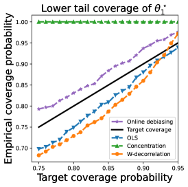
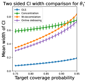
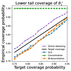
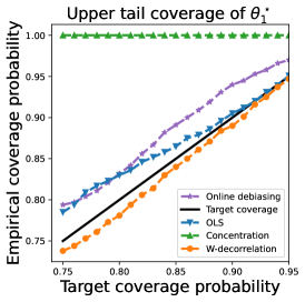
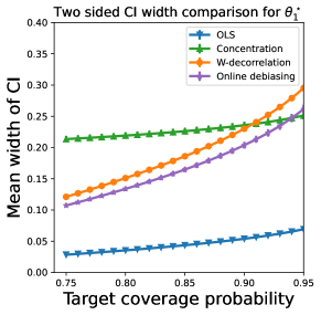
Figure 2: Average coverage and width of confidence intervals for $\theta_{1}^{*}$ across 1000 independent replications of a multi-armed bandit experiment (28) with ${\boldsymbol{\theta}^{*}}\equiv(\theta_{1}^{*},\theta_{2}^{*})=(0.3,0.3)^{\top}$. The covariates $\{\mathbf{x}_{i}\}_{i=1}^{1000}$ were selected using the UCB algorithm [20], and the error bars represent $\pm 1$ standard error. Left and Center: Coverage of one-sided $1-\alpha$ intervals for $\theta_{1}^{*}$. Right: Width of two-sided $1-\alpha$ intervals for $\theta_{1}^{*}$. The first row corresponds to data generated following the UCB algorithm, the second row corresponds to performances when additional data of size $\log^{2}(n)$ is added to the data; see Section 3.4.2. We observe that the online debiased estimator provide qualitatively similar performances in the both cases. See Section 4.1.1 for additional simulations.

4.2 Autoregressive time series model

Our next example involves estimating the parameters of an autoregressive time series model. It is well-known that the OLS estimate can exhibit non-Gaussian limit behavior for versions of such processes that are unstable [18]. In order to focus attention on the key issues, we restrict ourselves here to the simple case of a scalar autoregressive process.

More precisely, given the initial point $y_{0}=0$ and an unknown scalar $\theta^{*}\in(-1,1]$, consider a stochastic process generated by the first-order autoregression

$$y_{i}=\theta^{*}y_{i-1}+\mathbf{\epsilon}_{i}\quad\mbox{for $i=1,\ldots,n$.}$$ (33)

We assume that the noise sequence $\{\mathbf{\epsilon}_{i}\}_{i=1}^{n}$ consists of i.i.d. standard normal random variables. Note that the autoregression (33) is a special case of the stochastic linear regression model (1), in particular one with $x_{i}=y_{i-1}$ for all $i\in[n]$. An especially interesting instantiation of the autoregression (33) is obtained by setting $\theta^{*}=1$. Such a process is a special case of a unit root autoregression, a class of models that play an important role in econometric time series analysis [4].

With the choice $\theta^{*}=1$, the process (33) is a random walk and so has a variance that grows linearly with time. Moreover, by an application of Donsker’s theorem (cf. Example 3 in the paper [18]), we have

$$\frac{1}{n^{2}}\sum_{i=1}^{n}x_{i}^{2}:\,=\frac{1}{n^{2}}\sum_{i=1}^{n}y_{i-1}^{2} \stackrel{{\scriptstyle{\operatorname{d}}}}{{\longrightarrow}}\int_{0}^{1}\mathrm{w}^{2}(t)dt,\qquad\mbox{and}$$ (34)

$$\sqrt{\sum_{i=1}^{n}y_{i-1}^{2}}\cdot(\theta_{\scriptscriptstyle{\operatorname{LS}}}-\theta^{*}) \stackrel{{\scriptstyle{\operatorname{d}}}}{{\longrightarrow}}\frac{\mathrm{w}^{2}(1)-1}{2\int_{0}^{1}\mathrm{w}^{2}(t)dt},$$

where $\mathrm{w}(t)$ denotes the standard Wiener process (see the paper [28] for details). Put simply, in the autoregressive time series model (33) with ${\boldsymbol{\theta}^{*}}=1$ the stability condition (5) is not satisfied, and the distribution of the OLS estimate $\theta_{\scriptscriptstyle{\operatorname{LS}}}$ is not asymptotically normal.

In contrast to this negative result for the OLS estimate, we can show that the debiasing estimate $\widehat{\theta}_{\scriptscriptstyle{\operatorname{OD}}}$, after suitable centering and scaling, does indeed converge in distribution to a standard Gaussian. Our result is based on the tuning parameters and scaling matrices chosen as

$$\gamma_{n}=\frac{1}{(\log n)\cdot\log\log(n)},\quad\mbox{and}\quad{\mathbf{\Gamma}_{i,n}=\max\left\{(\log n)^{2}y_{i-1}^{2},\;\;\sum_{j=1}^{i-1}y_{j}^{2}\right\}}.$$ (35)

Corollary 2.

Given a sequence $\{y_{i}\}_{i=1}^{n}$ generated from the autoregressive model (33), the estimate $\widehat{\theta}_{\scriptscriptstyle{\operatorname{OD}}}$ (6) obtained with the tuning parameters (35) satisfies

$$\sqrt{\frac{\sum_{i=1}^{n}y_{i-1}^{2}}{(\log n)\cdot\log\log(n)}}\cdot(\widehat{\theta}_{\scriptscriptstyle{\operatorname{OD}}}-\theta^{*})\stackrel{{\scriptstyle{\operatorname{d}}}}{{\longrightarrow}}\mathcal{N}(0,1).$$ (36)

See Section 6.2 for the proof of this claim. 2 enables us to construct asymptotically exact confidence intervals for $\theta^{*}$. We also reiterate that the above result holds for any ${{\boldsymbol{\theta}^{*}}\in(-1,1]}$.

4.2.1 Numerical experiment

Figure 3 illustrates the performance of online debiasing with autoregression tuning (35). Here our data is generated from the time series model (33) with ${\boldsymbol{\theta}^{*}}=1$. We again find that online debiasing provides appropriate coverage for all confidence levels. Meanwhile, the OLS lower tail interval exhibits severe undercoverage, and W-decorrelation exhibits ranges of undercoverage for both tails. Finally, the concentration-based CI again provides 100% coverage for all confidence levels, at the expense of interval lengths that are uniformly longer than the online debiasing CIs.

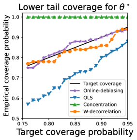
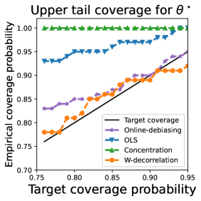
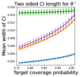
Figure 3: Average coverage and width of confidence intervals for ${\boldsymbol{\theta}^{*}}=1$ across 1000 independent replications of an autoregressive time series experiment (28). The error bars represent $\pm 1$ standard error. Left and Center: Coverage of one-sided $1-\alpha$ intervals for ${\boldsymbol{\theta}^{*}}$. Right: Width of two-sided $1-\alpha$ intervals for ${\boldsymbol{\theta}^{*}}$. See Section 4.2.1 for details.

4.3 Active learning with exploration

In our third example, we focus on the case where the covariates $\{\mathbf{x}_{i}\}_{i=1}^{n}$ are generated using any algorithm satisfying a sufficient exploration property.

Definition 4.1 (Selection algorithms with $\varepsilon$-exploration).

We say that a selection algorithm $\Psi_{n}=\{\psi_{i}\}_{i=1}^{n}$ admits a $\varepsilon$-exploration property if

$$\mathbf{x}_{i}:\,=\begin{cases}u_{i}&\text{with probability $1-\varepsilon_{i}$ for some $u_{i}\in\mathcal{F}_{i-1}$, and}\\ v_{i}&\mbox{with probability $\varepsilon_{i}$ for some $v_{i}$ independent of $\mathcal{F}_{i-1}$.}\end{cases}$$ (37)

Here the exploration probability sequence $\{\varepsilon_{i}\}_{i=1}^{n}$ consists of nonnegative scalars in the interval $(0,1)$, and the vectors $\{v_{i}\}_{i=1}^{n}$ are i.i.d. random vectors such that

$$\operatorname{\mathbb{E}}[v_{i}v_{i}^{\top}]\succeq\mathbf{G}\qquad\text{where}\quad\mathbf{G}\succeq\mathbf{0}$$ (38)

In words, the selection algorithm $\psi_{i}$ behaves as follows: with probability $1-\varepsilon_{i}$, it chooses vector $u_{i}$ based on the previous data points $\{(\mathbf{x}_{j},y_{j})\}_{j=1}^{i-1}$, and with probability $\varepsilon_{i}$, it chooses a random direction $v_{i}$, independent of the previous data points.

Example: $\varepsilon$-greedy linear bandits

Let us briefly consider a concrete instance of a selection algorithm $\{\psi_{i}\}_{i=1}^{n}$ that is of the $\varepsilon$-greedy type. In the linearly parameterized bandit problem, at each time $i\in[n]$, an algorithm $\psi_{i}$ chooses an action vector $\mathbf{x}_{i}$, usually lying within some bounded set $\mathcal{A}_{i}$, and obtains a reward $y_{i}=\big{\langle}\mathbf{x}_{i},{\boldsymbol{\theta}^{*}}\big{\rangle}+\epsilon_{i}$. A popular and simple strategy for regret minimization is a special case of the $\varepsilon$-greedy selection algorithm [20]. For linearly parameterized bandits, the selection algorithm $\psi_{i}$ chooses

$$\mathbf{x}_{i}\;\; \begin{cases}\in\arg\max\limits_{\mathbf{x}\in\mathcal{A}_{i}}\quad\big{\langle}\mathbf{x}_{i},\hat{\mathbf{\theta}}_{\text{ridge}}^{(i-1)}\big{\rangle}&\mbox{with probability $1-\varepsilon_{i}$, and}\\ \sim{\mathrm{Unif}}(\mathcal{A}_{i})&\mbox{with probability $\varepsilon_{i}$.}\end{cases}$$ (39)

where $\hat{\mathbf{\theta}}_{\text{ridge}}^{(i-1)}$ denotes the ridge regression estimator based on all data observed up to stage $i-1$, i.e., the collection of covariate-response pairs $\{(\mathbf{x}_{j},y_{j})\}_{j=1}^{i-1}$. Put simply, with probability $1-\varepsilon_{i}$, the selection algorithm $\psi_{i}$ chooses an optimal action given data collected so far (exploitation), and with probability $\varepsilon_{i}$, the algorithm randomizes uniformly amongst its choices (exploration). In the more general setting (37) considered here, it is not necessary to select the optimal action in the exploitation step. Rather, our result holds also when an arbitrary, $\mathcal{F}_{i-1}$-measurable choice is made in the first part of equation 39, as in the EXP3 or UCB algorithms with exploration. See the book [20] for more details. $\diamondsuit$

Returning to our general setting (37), we now state a guarantee for selection algorithms with $\varepsilon$-exploration. As is standard in the bandit literature, we assume that the covariates are uniformly bounded, so that there exists a scalar $K$ satisfying

$$\|\mathbf{x}_{i}\|_{2}\leq K\quad\mbox{for all $i\in[n]$.}$$ (40a)

See our discussion following the corollary for how this condition can be relaxed. In addition, we impose a sufficient exploration condition, meaning a lower bound on the magnitude of the exploration probabilities, of the form

$$\sum_{i=1}^{n}\varepsilon_{i}\geq\frac{\operatorname{\mathbb{E}}[\max_{i\in[n]}\|\mathbf{x}_{i}\|^{2}_{2}]}{\lambda_{\min}(\mathbf{G})}(\log n)^{2}$$ (40b)

where the reader should recall that the matrix $$\mathbf{G}$$ was defined in equation 38. We implement the debiasing estimate (6) with the choice of tuning parameters

$$\mathbf{\Gamma}_{i,n}=\sum_{j=1}^{n}\varepsilon_{j}\mathbf{G}\quad\quad\text{and}\quad\quad\gamma_{n}=\frac{1}{(\log n)\cdot\log\log(n)}.$$ (40c)

Corollary 3.

Suppose that Assumptions (A1) and (A2) hold, the covariates satisfy the bound (40a), and the exploration conditions (38) and (40b) both hold. Then given any consistent estimator ${\widehat{\sigma}}^{2}$ of the error variance $\sigma^{2}$, the estimator $\widehat{\boldsymbol{\theta}}_{\scriptscriptstyle{\operatorname{OD}}}$ with tuning parameters (40c) satisfies

$$\big{(}\log n\cdot\log\log(n)\cdot{\widehat{\sigma}}^{2}\big{)}^{-1/2}\cdot\mathbf{S}_{n}^{\frac{1}{2}}\left(\widehat{\boldsymbol{\theta}}_{\scriptscriptstyle{\operatorname{OD}}}-{\boldsymbol{\theta}^{*}}\right)\stackrel{{\scriptstyle{\operatorname{d}}}}{{\longrightarrow}}\mathcal{N}(0,\mathbf{I}).$$ (41a)

Moreover, for any $${\mathbf{v}}\in\bf{R}^{d} 1-\alpha {\mathbf{v}}^{\top}{\boldsymbol{\theta}^{*}}$$, the following is an asymptotically exact confidence intervals for

$$\left[\mathbf{e}_{1}^{\top}\widehat{\boldsymbol{\theta}}_{{\mathbf{v}},\scriptscriptstyle{\operatorname{diagOD}}}-\tfrac{\beta_{n}{\widehat{\sigma}}}{\sqrt{\gamma_{n}}}(\big{\langle}{\mathbf{v}},\mathbf{S}_{n}^{-1}{\mathbf{v}}\big{\rangle})^{\frac{1}{2}}z_{1-\alpha/2},\qquad\mathbf{e}_{1}^{\top}\widehat{\boldsymbol{\theta}}_{{\mathbf{v}},\scriptscriptstyle{\operatorname{diagOD}}}+\tfrac{\beta_{n}{\widehat{\sigma}}}{\sqrt{\gamma_{n}}}(\big{\langle}{\mathbf{v}},\mathbf{S}_{n}^{-1}{\mathbf{v}}\big{\rangle})^{\frac{1}{2}}z_{1-\alpha/2}\right],$$ (41b)

where $\beta_{n}=|\!|\!|\mathbf{D}_{{\mathbf{v}},n}^{-\frac{1}{2}}\mathbf{S}_{{\mathbf{v}},n}^{\frac{1}{2}}|\!|\!|_{{\scriptsize{\operatorname{op}}}}$ and the estimator $\widehat{\boldsymbol{\theta}}_{{\mathbf{v}},\scriptscriptstyle{\operatorname{diagOD}}}$ was calculated using (14) and with the tuning parameters (40c).

See Section 6.3 for the proof.

It is worth noting that the bounded covariate condition (40a) can be relaxed. For instance, in absence of the condition (40a), one may obtain a result similar to the part (a) of Corollary 3 under the following assumptions:

$$\gamma_{n}=o_{p}(\log\lambda_{\max}(\mathbf{S}_{n})),\quad\text{and}\quad\sum_{i=1}^{n}\varepsilon_{i}=\frac{\max_{i\in[n]}\operatorname{\mathbb{E}}[\|\mathbf{x}_{i}\|^{2}_{2}]}{\lambda_{\min}(\mathbf{G})\cdot o_{p}(\gamma_{n})}.$$

Finally, as a special case, Corollary 3 allows us to construct confidence interval for ${\mathbf{v}}^{\top}{\boldsymbol{\theta}^{*}}$ for multi-armed bandit problems that we discussed in Section 4.1. The condition (40a) is readily satisfied for multi-armed bandit problems, but the conditions (38) and (40b) are mildly stronger than the analogous condition (31).

4.3.1 Ensuring sufficient exploration via data augmentation

It is natural to ask if we can obtain online debiased method when the sufficient exploration condition is either difficult to verify or is not satisfied. In such settings, one simple fix is the following is based on the data-augmentation technique disscued in Section 3.4.2. Indeed, if we may collect $\log^{2}(n)$ many data points with $\mathbf{x}_{i}$ chosen uniformly at random froma $d$-dimensional unit sphere and append it to the new data. The new data-set has $n+\log^{2}(n)$ many data points, and the new dataset satisfy the exploration condition (37) with

$$\varepsilon_{i}=0\;\;\text{for all}\;\;1\leq i\leq n\qquad\varepsilon_{i}=1\;\;\text{for}\;\;i=n+1,\ldots,n+\log^{2}(n).$$

In summary, the growth condiiton (40b) is satisfied in this case up to a factor $d$. Hence, the result from Corollary 3 holds true in this case.

4.3.2 Numerical simulation

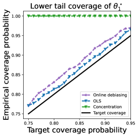
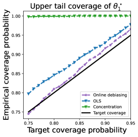
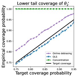
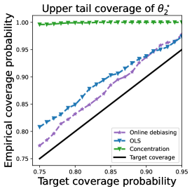
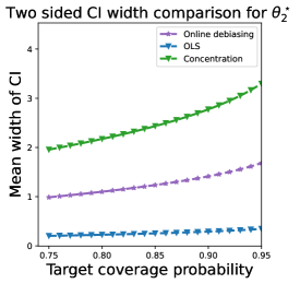
Figure 4: Average coverage and width of confidence intervals for $\theta_{1}^{*}$ and $\theta_{2}^{*}$ across 1000 independent replications of a linear bandits experiment (39) with ${\boldsymbol{\theta}^{*}}\equiv(\theta_{1}^{*},\theta_{2}^{*})=(0.3,0.3)^{\top}$. The covariates $\{\mathbf{x}_{i}\}_{i=1}^{1000}$ were selected using the $\varepsilon$-greedy linear bandits algorithm (39), and the error bars represent $\pm 1$ standard error. Left and Center: Coverage of one-sided $1-\alpha$ intervals for $\theta_{1}^{*}$ and $\theta_{2}^{*}$. Right: Width of two-sided $1-\alpha$ intervals for $\theta_{1}^{*}$ and $\theta_{2}^{*}$. See Section 4.3.2 for details.

Figure 4 illustrates the performance of online debiasing with the active learning tuning (40c). Here we consider a linear bandits problem with ${\boldsymbol{\theta}^{*}}=(0.3,0.3)^{\top}$ and i.i.d. standard normal error $\{\mathbf{\epsilon}_{i}\}_{i=1}^{n}$. The covariates $\{\mathbf{x}_{i}\}_{i=1}^{n}$ were generated using the $\varepsilon$-greedy linear bandits algorithm (39), where, for each stage, the context set $\mathcal{A}_{i}$ consisted of the same $50$ vectors drawn and uniformly from the unit sphere in dimension $2$. For this problem, the exploration lower bound equation 38 is satisfied with $\mathbf{G}=\frac{1}{|\mathcal{A}|}\cdot\sum_{\mathbf{a}_{i}\in\mathcal{A}}\mathbf{a}_{i}\mathbf{a}_{i}^{\top}$. In this setting, Abbasi-Yadkori, Pál and Szepesvári [2] only provide concentration-based CIs based on ridge regression estimators, rather than OLS. Here we report the CIs from ridge regression with regularization parameter $\lambda_{\text{Ridge}}=0.1$ (which closely approximates the OLS solution) and display analogous results for alternative regularization parameters in Appendix C.2. We computed the confidence intervals for $\theta_{1}^{*}$ and $\theta_{2}^{*}$ using Corollary 3.

We observe once more that online debiasing provides appropriate coverage for all confidence levels, while the OLS lower tail interval consistently undercovers. Meanwhile, the concentration CI provides high coverage for all confidence levels but yields intervals typically larger than the online debiasing CIs.

5 Proofs of the theorems

In this section, we provide the proofs of our two main results. We prove Theorem 1 in Section 5.1, and Theorem 2 in Section 5.2.

5.1 Proof of Theorem 1

Using the condition $\lambda_{\min}(\mathbf{S}_{n})\stackrel{{\scriptstyle{\operatorname{a.s.}}}}{{\longrightarrow}}\infty$ from assumption (A2), thus we may assume without loss of generality that $\mathbf{S}_{n}$ is invertible. We claim that it suffices to show that $\sqrt{\gamma_{n}}\cdot\mathbf{S}_{n}^{\frac{1}{2}}(\widehat{\boldsymbol{\theta}}_{\scriptscriptstyle{\operatorname{OD}}}-{\boldsymbol{\theta}^{*}})$ converges in distribution to ${\mathcal{N}}(0,\sigma^{2}\mathbf{I})$. Indeed, when this claim holds, then since ${\widehat{\sigma}}^{2}\stackrel{{\scriptstyle{\operatorname{p}}}}{{\longrightarrow}}\sigma^{2}$ by assumption, Slutsky’s theorem implies the claim of the theorem.

Recall from equation (10) that the random vector $\sqrt{\gamma_{n}}\cdot\mathbf{S}_{n}^{\frac{1}{2}}(\widehat{\boldsymbol{\theta}}_{\scriptscriptstyle{\operatorname{OD}}}-{\boldsymbol{\theta}^{*}})$ can be decomposed into the sum $\mathbf{b}_{n}+\mathbf{v}_{n}$. Based on this decomposition, we see that it is sufficient to prove that $\mathbf{b}_{n}\stackrel{{\scriptstyle{\operatorname{p}}}}{{\longrightarrow}}0$ and $\mathbf{v}_{n}\stackrel{{\scriptstyle{\operatorname{d}}}}{{\longrightarrow}}{\mathcal{N}}(0,\sigma^{2}\mathbf{I})$. The remainder of our proof is devoted to establishing these two claims.

Analysis of $\mathbf{b}_{n}$

By definition of the operator norm, we have the upper bound

$$\|\mathbf{b}_{n}\|_{2} \leq\sqrt{\gamma_{n}}\,|\!|\!|\mathbf{I}-\mathbf{W}_{n}\mathbf{X}_{n}\mathbf{S}_{n}^{-\frac{1}{2}}|\!|\!|_{{\scriptsize{\operatorname{op}}}}\big{\|}\mathbf{S}_{n}^{\frac{1}{2}}(\widehat{\boldsymbol{\theta}}_{\scriptscriptstyle{\operatorname{LS}}}-{\boldsymbol{\theta}^{*}})\big{\|}_{2}.$$ (42)

Lemma 1 from the paper [18] guarantees that

$$\big{\|}\mathbf{S}_{n}^{\frac{1}{2}}(\widehat{\boldsymbol{\theta}}_{\scriptscriptstyle{\operatorname{LS}}}-{\boldsymbol{\theta}^{*}})\big{\|}_{2} =O\left(\sqrt{\log\lambda_{\max}(\mathbf{S}_{n})}\right)\quad\text{almost surely}.$$ (43a)

On the other hand, the vanishing bias condition from Assumption (A3)(b) guarantees that

$$\sqrt{\gamma_{n}\log\lambda_{\max}(\mathbf{S}_{n})}\cdot|\!|\!|\mathbf{I}-\mathbf{W}_{n}\mathbf{X}_{n}\mathbf{S}_{n}^{-\frac{1}{2}}|\!|\!|_{{\scriptsize{\operatorname{op}}}}\stackrel{{\scriptstyle{\operatorname{p}}}}{{\longrightarrow}}0.$$ (43b)

Applying the bounds (43a) and (43b) to the right-hand side of the inequality (42) shows that $\|\mathbf{b}_{n}\|_{2}\stackrel{{\scriptstyle{\operatorname{p}}}}{{\longrightarrow}}0$.

Analysis of $\mathbf{v}_{n}$

In order to control the second term, we seek to apply a classical martingale central limit theorem (cf. Theorem 2.2 in the paper [8]). We begin by observing that $\{\sqrt{\gamma_{n}}\mathbf{w}_{i}\epsilon_{i}\}_{i=1}^{n}$ is a martingale difference sequence with respect to the sigma-field $\{\mathcal{F}_{i}\}_{i=1}^{n}$. Noting that the tuning parameter $\gamma_{n}$ is non-random, it follows that the sum $\sum_{i=1}^{n}\sqrt{\gamma_{n}}\mathbf{w}_{i}\epsilon_{i}$ has zero mean and moreover that

$$\sum_{i=1}^{n}\operatorname{\mathrm{Cov}}\left[\sqrt{\gamma_{n}}\mathbf{w}_{i}\epsilon_{i}\mid\mathcal{F}_{i-1}\right] =\gamma_{n}\sum_{i=1}^{n}\mathbf{w}_{i}\mathbf{w}_{i}^{\top}.$$ (44)

Consequently, in order to apply the martingale CLT so as to obtain the stated claim, we need to show that

$$\gamma_{n}\sum_{i=1}^{n}\mathbf{w}_{i}\mathbf{w}_{i}^{\top}\stackrel{{\scriptstyle{\operatorname{p}}}}{{\longrightarrow}}\sigma^{2}\mathbf{I}_{d}.$$

Doing so requires the following auxiliary lemma, which characterizes the behavior of the weight vector sequence $\{\mathbf{w}_{i}\}_{i=1}^{n}$ constructed in equation (7b).

Lemma 1.

Under the Assumption (A3) parts (a) and (c), the sequence of vectors $\{\mathbf{w}_{i}\}_{i=1}^{n}$ obtained from equation (7b) has the following properties:

(Stability:) $$\qquad\gamma_{n}\sum_{i=1}^{n}\mathbf{w}_{i}\mathbf{w}_{i}^{\top}\stackrel{{\scriptstyle{\operatorname{p}}}}{{\longrightarrow}}\mathbf{I}_{p},\quad\text{and}$$

(Vanishing norm:) $$\qquad\max_{i\in[n]}\sqrt{\gamma_{n}}\|\mathbf{w}_{i}\|_{2}\stackrel{{\scriptstyle{\operatorname{p}}}}{{\longrightarrow}}0.$$

See Appendix B for the proof of this lemma.

With the above lemma in hand, we now apply a standard martingale central limit theorem to conclude that

$$\sum_{i=1}^{n}\sqrt{\gamma_{n}}\mathbf{w}_{i}\epsilon_{i}\stackrel{{\scriptstyle{\operatorname{d}}}}{{\longrightarrow}}\mathcal{N}(0,\sigma^{2}\mathbf{I}_{d}).$$

Putting together the pieces, we conclude that

$$\sqrt{\gamma_{n}}\cdot\mathbf{S}_{n}^{\frac{1}{2}}(\widehat{\boldsymbol{\theta}}_{\scriptscriptstyle{\operatorname{OD}}}-\theta)=\mathbf{b}_{n}+\sum_{i=1}^{n}\sqrt{\gamma_{n}}\mathbf{w}_{i}\epsilon_{i}\stackrel{{\scriptstyle{\operatorname{d}}}}{{\longrightarrow}}\mathcal{N}(0,\sigma^{2}\mathbf{I}_{d}),$$

which completes the proof of Theorem 1.

5.1.1 Proof of claim (23):

For simplicity, let us assume $\sigma$ is known. Recalling the decomposition (10) we have

$$\gamma_{n}\cdot\|\widehat{\boldsymbol{\theta}}_{\scriptscriptstyle{\operatorname{OD}}}-{\boldsymbol{\theta}^{*}}\|_{\mathbf{S}_{n}}^{2} =\|\mathbf{b}_{n}\|^{2}+2\big{\langle}\mathbf{b}_{n},\mathbf{v}_{n}\big{\rangle}+\|\mathbf{v}_{n}\|^{2}$$

$$\leq\|\mathbf{b}_{n}\|^{2}+2\|\mathbf{b}_{n}\|\cdot\|\mathbf{v}_{n}\|+\|\mathbf{v}_{n}\|^{2}$$

Invoking the condition $\sqrt{\gamma_{n}\log\lambda_{\max}(\mathbf{S}_{n})}\cdot|\!|\!|\mathbf{I}-\mathbf{W}_{n}\mathbf{X}_{n}\mathbf{S}_{n}^{-\frac{1}{2}}|\!|\!|_{{\scriptsize{\operatorname{op}}}}\stackrel{{\scriptstyle L_{1}}}{{\longrightarrow}}0$ we immediately have $\|\mathbf{b}_{n}\|^{2}\stackrel{{\scriptstyle L_{1}}}{{\longrightarrow}}0$. It suffices to show that $\|\mathbf{v}_{n}\|^{2}\leq d$ and $\operatorname{\mathbb{E}}[\|\mathbf{v}_{n}\|^{2}]\rightarrow d$. Observe that

$$\operatorname{\mathbb{E}}[\|\mathbf{v}_{n}\|^{2}] =\gamma_{n}\cdot\sum_{i=1}^{n}\operatorname{\mathbb{E}}[\mathbf{\epsilon}_{i}^{2}\|\mathbf{w}_{i}\|^{2}]+\sum_{i\neq j}\gamma_{n}\cdot\operatorname{\mathbb{E}}[\mathbf{\epsilon}_{i}\mathbf{\epsilon}_{j}\mathbf{w}_{i}^{\top}\mathbf{w}_{j}]$$

$$\stackrel{{\scriptstyle(i)}}{{=}}\sum_{i=1}^{n}\gamma_{n}\cdot\sigma^{2}\cdot\operatorname{\mathbb{E}}[\|\mathbf{w}_{i}\|^{2}]+\sum_{i\neq j}\gamma_{n}\cdot\operatorname{\mathbb{E}}[\mathbf{\epsilon}_{i}\mathbf{\epsilon}_{j}\mathbf{w}_{i}^{\top}\mathbf{w}_{j}]$$

The last line above follows from the assumption $\operatorname{\mathbb{E}}[\mathbf{\epsilon}_{i}^{2}\mid\mathcal{F}_{i-1}]=\sigma^{2}$ and the fact (by construction) that $\mathbf{w}_{i}\in\mathcal{F}_{i-1}$. Taking trace on both sides of equation (65) we have that $\gamma_{n}\cdot\|\mathbf{w}_{i}\|^{2}\leq d$, and using the stronger $L_{1}$ version of assumption (A3) along with the proof techniques of Lemma 1 we have $\gamma_{n}\cdot\sum_{i=1}^{n}\operatorname{\mathbb{E}}[\|\mathbf{w}_{i}\|^{2}]\rightarrow\sigma^{2}d$. It remains to show that $\operatorname{\mathbb{E}}[\mathbf{\epsilon}_{i}\mathbf{\epsilon}_{j}\mathbf{w}_{i}^{\top}\mathbf{w}_{j}]=0$ for all $i\neq j$. Without loss of generality, assume $i<j$. By construction of $\mathbf{w}_{i}$ and the martingale assumption (A1) of the noise $\mathbf{\epsilon}_{i}$, we have $\{\mathbf{w}_{i},\mathbf{w}_{j},\mathbf{\epsilon}_{i}\}\in\mathcal{F}_{j-1}$. As a result, we conclude that

$$\operatorname{\mathbb{E}}[\mathbf{\epsilon}_{i}\mathbf{\epsilon}_{j}\mathbf{w}_{i}^{\top}\mathbf{w}_{j}]=\operatorname{\mathbb{E}}\Big{[}\mathbf{\epsilon}_{i}\cdot\mathbf{w}_{i}^{\top}\mathbf{w}_{j}\operatorname{\mathbb{E}}[\mathbf{\epsilon}_{j}\mid\mathcal{F}_{j-1}]\Big{]}=0,$$

thereby completing the proof of the claim (23).

5.2 Proof of Theorem 2

We prove part (a) of Theorem 2 in Section 5.2.1 and part (b) of Theorem 2 in Section 5.2.3.

5.2.1 Proof of Theorem 2(a)

Throughout the proof, we use ${\widehat{\boldsymbol{\theta}}}$ to denote a generic estimator for ${\boldsymbol{\theta}^{*}}$. We assume that the estimator ${\widehat{\boldsymbol{\theta}}}$ is a function only of the $n$ datapoints $\{(\mathbf{x}_{i},y_{i})\}_{i=1}^{n}$ and family of selection algorithms $\Psi_{n}:\,=(\psi_{i})_{i\in[n]}$, one for each $i\in[n]$; of course, the estimator ${\widehat{\boldsymbol{\theta}}}$ does not know the value of the true parameter ${\boldsymbol{\theta}^{*}}$. Consider any positive semidefinite and potentially data-dependent matrix ${\mathbf{M}}\in{\mathbb{R}}^{d\times d}$, and define the nonnegative scalar loss function

$$\mathrm{\ell}_{\mathbf{M}}({\widehat{\boldsymbol{\theta}}},{\boldsymbol{\theta}^{*}}) :\,=({\widehat{\boldsymbol{\theta}}}-{\boldsymbol{\theta}^{*}})^{\top}{\mathbf{M}}({\widehat{\boldsymbol{\theta}}}-{\boldsymbol{\theta}^{*}}).$$ (45)

From minimax to Bayes risk

In terms of the above notations, Theorem 2 (a) posits a lower bound on the minimax risk:

$$\inf_{{\widehat{\boldsymbol{\theta}}}}\sup_{{\boldsymbol{\theta}^{*}}\in\bf{R}^{d}}\;\operatorname{\mathbb{E}}[\mathrm{\ell}_{\mathbf{M}}({\widehat{\boldsymbol{\theta}}},{\boldsymbol{\theta}^{*}})\mid{\boldsymbol{\theta}^{*}}],$$ (46)

where in the above expression, we have taken an expectation of the loss $\mathrm{\ell}_{\mathbf{M}}({\widehat{\boldsymbol{\theta}}},{\boldsymbol{\theta}^{*}})$ over the randomness in the data $(\mathbf{X}_{n},\mathbf{y}_{n})$ conditioned on ${\boldsymbol{\theta}^{*}}$. We establish the lower bound Theorem 2(a) on the minimax risk (46) via the standard avenue of first lower bounding the minimax risk by the Bayes risk, and then providing a lower bound on the Bayes risk. In order to do so, we make use of the inequality

$$\inf_{{\widehat{\boldsymbol{\theta}}}}\sup_{{\boldsymbol{\theta}^{*}}}\;\operatorname{\mathbb{E}}[\mathrm{\ell}_{\mathbf{M}}({\widehat{\boldsymbol{\theta}}},{\boldsymbol{\theta}^{*}})\mid{\boldsymbol{\theta}^{*}}]\geq\inf_{{\widehat{\boldsymbol{\theta}}}}\;\operatorname{\mathbb{E}}_{{\boldsymbol{\theta}^{*}},\mathbf{X}_{n},\mathbf{y}_{n}}\mathrm{\ell}_{\mathbf{M}}({\widehat{\boldsymbol{\theta}}},{\boldsymbol{\theta}^{*}}),$$ (47)

where the expectation $\operatorname{\mathbb{E}}_{{\boldsymbol{\theta}^{*}},\mathbf{X}_{n},\mathbf{y}_{n}}$ above is taken with respect the joint distribution on $({\boldsymbol{\theta}^{*}},\mathbf{X}_{n},\mathbf{y}_{n})$. Note that this joint distribution is defined by choosing a prior distribution over the parameter ${\boldsymbol{\theta}^{*}}$, and this choice of prior is a design parameter in our proof.

Main argument

We claim that it suffices to prove that for any estimator ${\widehat{\boldsymbol{\theta}}}$

$$\operatorname{\mathbb{E}}[\mathrm{\ell}_{\mathbf{M}}({\widehat{\boldsymbol{\theta}}},{\boldsymbol{\theta}^{*}})\mid\mathbf{X}_{n},\mathbf{y}_{n}]\geq\sigma^{2}\operatorname{trace}({\mathbf{M}}\mathbf{S}_{n}^{-1}).$$ (48)

where the expectation $\operatorname{\mathbb{E}}[\cdot\mid\mathbf{X}_{n},y_{n}]$ is taken with respect to the conditional distribution of ${\boldsymbol{\theta}^{*}}\mid\mathbf{X}_{n},y_{n}$. Indeed, taking expectation over $\mathbf{X}_{n},y_{n}$ yields the desired bound:

$$\operatorname{\mathbb{E}}_{{\boldsymbol{\theta}^{*}},\mathbf{X}_{n},\mathbf{y}_{n}}\mathrm{\ell}_{\mathbf{M}}({\widehat{\boldsymbol{\theta}}},{\boldsymbol{\theta}^{*}}) =\operatorname{\mathbb{E}}_{\mathbf{X}_{n},\mathbf{y}_{n}}\operatorname{\mathbb{E}}[\mathrm{\ell}_{\mathbf{M}}({\widehat{\boldsymbol{\theta}}},{\boldsymbol{\theta}^{*}})\mid\mathbf{X}_{n},\mathbf{y}_{n}]\geq\sigma^{2}\operatorname{\mathbb{E}}_{\mathbf{X}_{n},\mathbf{y}_{n}}\operatorname{trace}({\mathbf{M}}\mathbf{S}_{n}^{-1}).$$ (49)

Accordingly, it remains to prove the bound (48).

Proof of bound (48)

We complete the proof of this bound by first computing the conditional distribution of ${\boldsymbol{\theta}^{*}}\mid\mathbf{X}_{n},\mathbf{y}_{n}$, and then lower bounding the conditional expectation of the loss $\mathrm{\ell}_{\mathbf{M}}({\widehat{\boldsymbol{\theta}}},{\boldsymbol{\theta}^{*}})$ given the data $(\mathbf{X}_{n},y_{n})$. Concretely, we show that under the prior distribution ${\boldsymbol{\theta}^{*}}\sim\mathcal{N}(0,\rho^{2}\mathbf{I}_{d})$, we have

$${\boldsymbol{\theta}^{*}}\mid\mathbf{X}_{n},\mathbf{y}_{n} \sim\mathcal{N}(\mu_{n},\mathbf{\Sigma}_{n}),\quad\text{where}$$

$$\mu_{n}=\mathbf{\Sigma}_{n}\mathbf{X}_{n}\mathbf{y}_{n}\quad \text{and}\quad\mathbf{\Sigma}_{n}=(\mathbf{S}_{n}/\sigma^{2}+\mathbf{I}_{d}/\rho^{2})^{-1}.$$ (50)

A simple calculation using these distributional properties yields that for any positive semidefinite matrix ${\mathbf{M}}$—one that may depend on the data $(\mathbf{X}_{n},y_{n})$—the function $\theta\mapsto\operatorname{\mathbb{E}}[\mathrm{\ell}_{\mathbf{M}}(\theta,{\boldsymbol{\theta}^{*}})\mid\mathbf{X}_{n},\mathbf{y}_{n}]$ is minimized by the choice ${\widehat{\boldsymbol{\theta}}}:\,=\mathbf{\Sigma}_{n}\mathbf{X}_{n}\mathbf{y}_{n}$. Moreover, this choice of estimator yields the minimum value $\sigma^{2}\operatorname{trace}({\mathbf{M}}\mathbf{\Sigma}_{n})$. Finally, we are free to choose the value of the prior error variance $\rho^{2}$; in particular, taking the limit $\rho^{2}\rightarrow\infty$ yields the claim (48).

It remains to prove the auxiliary claim (5).

Proof of claim (5)

We proceed via induction on the number of datapoints $n$.

Base case

For $n=0$, we have

$${\boldsymbol{\theta}^{*}}\mid\mathbf{X}_{0},\mathbf{y}_{0}\equiv{\boldsymbol{\theta}^{*}}\sim\mathcal{N}(0,\rho^{2}\mathbf{I}_{d}),$$ (51)

using the facts that ${\boldsymbol{\theta}^{*}}\sim\mathcal{N}(0,\rho^{2}\mathbf{I}_{d})$ by our choice of prior, and the triple $(\mathbf{X}_{0},\mathbf{y}_{0},\mathbf{S}_{0})$ are defined as zeros of respective dimensions. This proves the statement (5) for $n=0$, and $\mu_{0}=0$, and $\mathbf{\Sigma}_{0}=\rho^{2}\mathbf{I}_{d}$.

Induction step

Given some $n\geq 1$, assume that the claim (5) holds for $n-1$. Here we show that the statement then holds for $n$. Recall that the query algorithm $\psi_{i}:({\mathbb{R}}\times{\mathbb{R}}^{d})^{i-1}\to{\mathbb{R}}^{d}$ is oblivious to the true value ${\boldsymbol{\theta}^{*}}$; thus, the conditional distribution $\mathbf{x}_{n}\mid\mathcal{F}_{n}$ is independent of ${\boldsymbol{\theta}^{*}}$ (see the discussion before Theorem 2). Furthermore, from the model (1), it follows that the conditioned random variable $y_{n}\mid\mathcal{F}_{n-1},\mathbf{x}_{n},{\boldsymbol{\theta}^{*}}$ follows a $\mathcal{N}(\mathbf{x}_{n}^{\top}{\boldsymbol{\theta}^{*}},\sigma^{2})$ distribution, and using the induction hypothesis (5), we conclude that ${\boldsymbol{\theta}^{*}}\mid\mathbf{X}_{n-1},y_{n-1}\sim\mathcal{N}(\mu_{n-1},\mathbf{\Sigma}_{n-1})$.

Now let $\frac{d\mathbb{P}({\boldsymbol{\theta}^{*}}\mid\mathbf{X}_{n},\mathbf{y}_{n})}{d\nu^{d}({\boldsymbol{\theta}^{*}})}$ denote the Radon-Nikodym derivative of the conditional distribution defind by ${\boldsymbol{\theta}^{*}}\mid\mathbf{X}_{n},y_{n}$ with respect to the Lebesgue measure $\nu^{d}$ on $\bf{R}^{d}$. With the last three observations in hand, an application of Bayes’ rule yields

$$\frac{d\mathbb{P}({\boldsymbol{\theta}^{*}}\mid\mathbf{X}_{n},\mathbf{y}_{n})}{d\nu^{d}({\boldsymbol{\theta}^{*}})} \propto\exp\left\{-\frac{1}{2}({\boldsymbol{\theta}^{*}}-\mu_{n-1})^{\top}\mathbf{\Sigma}_{n-1}^{-1}({\boldsymbol{\theta}^{*}}-\mu_{n-1})^{\top}\right\}\times\exp\left\{-\frac{1}{2\sigma^{2}}(y_{n}-\mathbf{x}_{n}^{\top}{\boldsymbol{\theta}^{*}})^{2}\right\}$$

$$\propto\exp\left\{-\frac{1}{2}({\boldsymbol{\theta}^{*}}-\mu_{n})^{\top}\mathbf{\Sigma}_{n}({\boldsymbol{\theta}^{*}}-\mu_{n})^{\top}\right\},$$

where the pair $(\mu_{n},\mathbf{\Sigma}_{n})$ are given by

$$\mathbf{\Sigma}_{n}^{-1}=\mathbf{\Sigma}_{n-1}^{-1}+\frac{\mathbf{x}_{n}\mathbf{x}_{n}^{\top}}{\sigma^{2}}\quad\text{and}\quad\mu_{n}=\frac{1}{\sigma^{2}}\mathbf{\Sigma}_{n}\sum_{i=1}^{n}\mathbf{x}_{i}y_{i}.$$

This completes the proof of the inductive step, and putting together the pieces yields the claim of part (a) of 2.

5.2.2 Proof of Theorem 2(b)

This proof and construction follows by discretizing the construction in [19], which establishes a similar result in a kernelized version of the problem in continuous time. Regrettably, the error terms that arise as a consequence of the discretization lead to a rather unpleasant calculation. We may assume without loss of generality that $\sigma=1$. The general result with $\sigma>0$ can be obtained by a rescaling argument. For simplicity we also assume that $n$ is divisible by $d-1$, which can be relaxed by correctly rounding the indices of the many sums that appear in the calculations that follow. Let $d>1$ and ${\mathbf{v}}=e_{d}=(\bm{0},1)^{\top}\in{\mathbb{R}}^{d}$. Our proof follows a standard Bayesian argument. Consider a randomly generated vector ${\boldsymbol{\theta}^{*}}$ that is equal to $\bm{0}$ with probability $1/2$, and otherwise sampled from a multivariate Gaussian distribution with mean $\mu=(\bm{0},1)^{\top}\in{\mathbb{R}}^{d}$ and degenerate covariance

$$\Sigma=\begin{pmatrix}\mathbf{I}&\bm{0}\\ \bm{0}^{\top}&0\end{pmatrix}\,.$$

Lower bounding the supremum by an expectation over this prior, the minimax risk can be lower bounded as

$$\inf_{{\widehat{U}}}\sup_{{\boldsymbol{\theta}^{*}}}{\operatorname{\mathbb{E}}}_{{\boldsymbol{\theta}^{*}}}\left[\frac{(\langle{\mathbf{v}},{\boldsymbol{\theta}^{*}}\rangle-{\widehat{U}})^{2}}{\|{\mathbf{v}}\|^{2}_{\mathbf{S}_{n}^{-1}}}\right]\geq\inf_{{\widehat{U}}}{\operatorname{\mathbb{E}}}\left[\frac{(\langle{\mathbf{v}},{\boldsymbol{\theta}^{*}}\rangle-{\widehat{U}})^{2}}{\|{\mathbf{v}}\|^{2}_{\mathbf{S}_{n}^{-1}}}\right]\,.$$ (52)

where the second expectation integrates over randomness in ${\boldsymbol{\theta}^{*}}$ as well as the observations $\{(\mathbf{x}_{i},y_{i})\}_{i\in[n]}$.

We now provide a sequential definition of the selection algorithm that yields the claimed lower bound. Each covariate $\mathbf{x}_{i}$ is supported on the last coordinate as well as one of the first $d-1$ coordinates, chosen in round-robin fashion. Let $u_{i}=1+(i\operatorname{mod}(d-1))$ and $v_{i}=\left\lceil i/(d-1)\right\rceil$, which are chosen so that

$$\{u_{i}\}_{i\geq 1}=\{1,2,\ldots,d-1,1,2,\ldots\}\text{ and }\{v_{i}\}_{i\geq 1}=\{\underbrace{1,1,\ldots,1}_{d-1\text{ times}},2,2,\ldots\}\,.$$

In other words, $u_{i}$ is the index of the first non-zero coordinate in $\mathbf{x}_{i}$ and $v_{i}$ is the number of times coordinate $u_{i}$ was non-zero in rounds $j\leq i$. The first $d-1$ coordinates of the covariate process are deterministic and the last coordinate is chosen adaptively to maximize the difficulty of estimation. Precisely, $\{\mathbf{x}_{i}\}_{i\geq 1}$ is given by

$$\mathbf{x}_{i}:\,=b_{v_{i}}e_{u_{i}}+a_{u_{i},v_{i}}e_{d}\in{\mathbb{R}}^{d}\,,$$

where $b_{v}:\,=v^{-1/4}/\sqrt{d}$, and the random sequence $\{a_{u,v}\}_{u\in\{1,\ldots,d-1\},v\geq 1}$ is to defined momentarily. Let $y_{u,w}:\,=y_{u+(w-1)(d-1)}$, which is the observed response in the round $i$ where coordinate $u$ was non-zero for the $v$th time. Define

$$m_{u,v}:\,=\sum_{w=1}^{v}b_{w}(y_{u,w}-a_{u,w}),\quad\mbox{and}\quad d_{v}:\,=1+\sum_{w=1}^{v}b_{w}^{2}.$$

Then $a_{u,v}:\,=-b_{v}m_{u,v-1}/d_{v-1}$, noting that $a_{u,1}=0$ for all $u$.

To provide some intuition, our construction is designed so as to make estimation challenging. Let $\mathbf{\epsilon}_{u,v}=\mathbf{\epsilon}_{u+(v-1)(d-1)}$. On the event that ${\boldsymbol{\theta}^{*}}\neq\bm{0}$, we have the equality $y_{u,v}=a_{u,v}+\theta^{*}_{u}b_{v}+\epsilon_{u,v}$, and the ratio $m_{u,v}/d_{v}$ is the ridge regression estimate of $\theta^{*}_{u}$. For any vector ${\boldsymbol{\theta}^{*}}\neq 0$, the choice $\mathbf{x}_{i}$ ensures that

$$\langle\mathbf{x}_{i},{\boldsymbol{\theta}^{*}}\rangle=a_{u_{i},v_{i}}+b_{v_{i}}\theta^{*}_{u_{i}}\approx 0=\langle\mathbf{x}_{i},\bm{0}\rangle\,,$$

so that the observed responses are extremely similarly under either of the events $\{{\boldsymbol{\theta}^{*}}=\bm{0}\}$ or $\{{\boldsymbol{\theta}^{*}}\neq\bm{0}\}$. But $\langle{\mathbf{v}},{\boldsymbol{\theta}^{*}}\rangle=\bm{1}({\boldsymbol{\theta}^{*}}\neq\bm{0})$, which means that any estimator of $\langle{\mathbf{v}},{\boldsymbol{\theta}^{*}}\rangle$ must have large error in expectation. What is missing is to formalize the above claims and show that $\|{\mathbf{v}}\|^{2}_{\mathbf{S}^{-1}_{n}}$ shrinks suitably fast.

Returning the proof, since $\|{\mathbf{v}}\|^{2}_{\mathbf{S}_{n}^{-1}}$ is $\mathcal{F}_{n}$-measurable, the infimum on the right-hand side of equation (52) is achieved by the estimator

$${\widehat{U}}_{n}:\,={\operatorname{\mathbb{E}}}[\langle{\mathbf{v}},{\boldsymbol{\theta}^{*}}\rangle|\mathcal{F}_{n}]=\mathbb{P}\left({\boldsymbol{\theta}^{*}}\neq\bm{0}|\mathcal{F}_{n}\right).$$

Therefore, introducing the event $\mathcal{E}=\{{\boldsymbol{\theta}^{*}}\neq\bm{0}\}$, we have the lower bound

Risk $$\geq{\operatorname{\mathbb{E}}}\Biggr{[}\frac{\big{(}\mathbb{P}\big{[}{\boldsymbol{\theta}^{*}}\neq\bm{0}\mid\mathcal{F}_{n}\big{]}-\langle e_{d},{\boldsymbol{\theta}^{*}}\rangle\big{)}^{2}}{\|e_{d}\|^{2}_{\mathbf{S}_{n}^{-1}}}\Biggr{]}={\operatorname{\mathbb{E}}}\Biggr{[}\frac{{\widehat{U}}_{n}(1-{\widehat{U}}_{n})}{\|e_{d}\|^{2}_{\mathbf{S}_{n}^{-1}}}\Biggr{]}\geq\frac{1}{2}{\operatorname{\mathbb{E}}}\Biggr{[}\frac{{\widehat{U}}_{n}(1-{\widehat{U}}_{n})}{\|e_{d}\|^{2}_{\mathbf{S}_{n}^{-1}}}\Bigg{|}\mathcal{E}\Biggr{]}\,.$$

In the remainder of the proof, we study the laws of ${\widehat{U}}_{n}$ and $\smash{\|e_{d}\|^{2}_{\mathbf{S}_{n}^{-1}}}$ under the measure $\mathbb{P}(\cdot\mid\mathcal{E})$. For a sequence of random variables $X_{n}$, we use the notation $X_{n}=\Omega_{p}(a_{n})$ to mean that $\sup_{n}\mathbb{P}(X_{n}/a_{n}<C_{\epsilon}\mid\mathcal{E})<\epsilon$. We will show below that

$${\widehat{U}}_{n}(1-{\widehat{U}}_{n}) =\Omega_{p}(1),\qquad\mbox{and}$$ (53a)

$$\frac{1}{\|e_{d}\|_{\mathbf{S}_{n}^{-1}}^{2}} =\Omega_{p}(d\log(n/d^{3}))\,.$$ (53b)

Therefore, there exists a universal constant $C>0$ such that for $n\geq d^{3}/C$,

$$\mathbb{P}\left(1/\|e_{d}\|_{\mathbf{S}_{n}^{-1}}^{2}\geq Cd\log(n)\right)\geq 3/4\text{ and }\mathbb{P}\left({\widehat{U}}_{n}(1-{\widehat{U}}_{n})\geq C\right)\geq 3/4\,.$$

By a union bound and the positivity in the integrand of the risk,

Risk $$\geq\frac{C^{2}d\log(n/d^{3})}{4}\,.$$

It remains to show that the lower bounds (53a) and (53b) hold, which we prove in Appendix F.

5.2.3 Proof of 2(c)

Let $\operatorname{\mathbb{E}}_{\boldsymbol{\theta}}$ denote expectation over a data set drawn from the distribution indexed by $\boldsymbol{\theta}$, and define $\mathbb{P}_{\boldsymbol{\theta}}$ as the analogous probability. For a given dataset based on $n$ samples, consider a confidence interval of the form $[\widehat{\ell}_{n},\widehat{u}_{n}]$. Introducing the shorthand $\xi_{n}^{2}:\,=v^{T}\mathbf{S}_{n}^{-1}v$, we then define the minimax risk

$${\sf Risk} :\,=\inf_{[\widehat{\ell}_{n},\widehat{u}_{n}]}\sup_{{\boldsymbol{\theta}^{*}}}\operatorname{\mathbb{E}}_{\boldsymbol{\theta}^{*}}\bigg{\{}\frac{\widehat{u}_{n}-\widehat{\ell}_{n}}{\xi_{n}}\bigg{\}},$$

where we take the infimum over all estimators $[\widehat{\ell}_{n},\widehat{u}_{n}]$ such that $\mathbb{P}_{{\boldsymbol{\theta}^{*}}}\big{(}[\widehat{\ell}_{n},\widehat{u}_{n}]\ni v^{\top}{\boldsymbol{\theta}^{*}}\big{)}\geq 1-\alpha$ for each value of ${\boldsymbol{\theta}^{*}}$.

By the usual Bayesian argument, for any prior distribution $\pi$ on ${\boldsymbol{\theta}^{*}}$, we have the lower bound

$${\sf Risk}\geq\inf_{[\widehat{\ell}_{n},\widehat{u}_{n}]}{\operatorname{\mathbb{E}}}_{{\boldsymbol{\theta}^{*}}\sim\pi}\operatorname{\mathbb{E}}_{\boldsymbol{\theta}^{*}}\bigg{[}\frac{\widehat{u}_{n}-\widehat{\ell}_{n}}{\xi_{n}}\bigg{]}.$$

We now obtain a further lower bound by enlarging the space of possible estimators $[\widehat{\ell}_{n},\widehat{u}_{n}]$, in particular requiring only that $[\widehat{\ell}_{n},\widehat{u}_{n}]$ belong to the set

$$\mathcal{A} :\,=\Big{\{}[\widehat{\ell}_{n},\widehat{u}_{n}]\;\mid\;\operatorname{\mathbb{E}}_{{\boldsymbol{\theta}^{*}}\sim\pi}\mathbb{P}_{\boldsymbol{\theta}^{*}}\big{(}[\widehat{\ell}_{n},\widehat{u}_{n}]\ni v^{\top}{\boldsymbol{\theta}^{*}}\big{)}\geq 1-\alpha\Big{\}}.$$

Since this allows for a larger collection of possible estimators, we have the lower bound

$${\sf Risk} \geq\inf_{[\widehat{\ell}_{n},\widehat{u}_{n}]\in\mathcal{A}}{\operatorname{\mathbb{E}}}_{{\boldsymbol{\theta}^{*}}\sim\pi}\operatorname{\mathbb{E}}_{\boldsymbol{\theta}^{*}}\bigg{\{}\frac{\widehat{u}_{n}-\widehat{\ell}_{n}}{\xi_{n}}\bigg{\}}.$$

We are now free to choose the prior. In particular, we set $\pi$ equal to the density $\phi_{\rho}$ of the Gaussian random vector $\mathcal{N}(0,\rho^{2}\mathbf{I}_{d})$. From our previous calculations (5) we have that conditional on the observed data, the random vector ${\boldsymbol{\theta}^{*}}$ is Gaussian with covariance $(\mathbf{S}_{n}/\sigma^{2}+\mathbf{I}_{d}/\rho^{2})^{-1}$. With this choice, the random variable $v^{\top}{\boldsymbol{\theta}^{*}}$, conditioned on the observed data, is a Gaussian random variable with variance $\tilde{v}_{n}^{2}:\,=v^{T}(\mathbf{S}_{n}/\sigma^{2}+\mathbf{I}_{d}/\rho^{2})^{-1}v$. Therefore, the width of any confidence interval $[\widehat{\ell}_{n},\widehat{u}_{n}]\in\mathcal{A}$ is lower bounded by $2z_{1-\alpha/2}\tilde{v}_{n}$, and we have

$${\sf Risk} \geq 2z_{1-\alpha/2}{\operatorname{\mathbb{E}}}_{{\boldsymbol{\theta}^{*}}\sim\pi}\operatorname{\mathbb{E}}_{\boldsymbol{\theta}^{*}}\Big{[}\frac{\tilde{v}_{n}}{\xi_{n}}\Big{]}.$$

It remains to show that $\lim_{\rho\to\infty}{\operatorname{\mathbb{E}}}_{{\boldsymbol{\theta}^{*}}\sim\pi}\operatorname{\mathbb{E}}_{\boldsymbol{\theta}^{*}}\big{[}\frac{\tilde{v}_{n}}{\xi_{n}}\big{]}=1$. Recalling that $\phi_{\rho}$ denotes the Gaussian density with zero mean and covariance $\rho^{2}I_{d}$, we have

$${\operatorname{\mathbb{E}}}_{{\boldsymbol{\theta}^{*}}\sim\pi}\operatorname{\mathbb{E}}_{\boldsymbol{\theta}^{*}}\Big{[}\frac{\tilde{v}_{n}}{\xi_{n}}-1\Big{]} =\int\operatorname{\mathbb{E}}_{\boldsymbol{\theta}^{*}}\Big{[}\frac{\tilde{v}_{n}}{\xi_{n}}-1\Big{]}\phi_{\rho}({\boldsymbol{\theta}^{*}})d{\boldsymbol{\theta}^{*}},$$

By the bounded convergence theorem, we have

$$\lim_{\rho\to\infty}\operatorname{\mathbb{E}}_{\boldsymbol{\theta}^{*}}\Big{[}\frac{\tilde{v}_{n}}{\xi_{n}}-1\Big{]} =0,$$

pointwise for each $\boldsymbol{\theta}$. Consequently, the quantity in the integral converges point-wise to zero, so that applying the bounded convergence theorem again yields

$$\lim_{\rho\to\infty}{\operatorname{\mathbb{E}}}_{{\boldsymbol{\theta}^{*}}\sim\pi}\operatorname{\mathbb{E}}_{\boldsymbol{\theta}^{*}}\Big{[}\frac{\tilde{v}_{n}}{\xi_{n}}-1\Big{]}=\lim_{\rho\to\infty}\int\operatorname{\mathbb{E}}_{\boldsymbol{\theta}^{*}}\Big{[}\frac{\tilde{v}_{n}}{\xi_{n}}-1\Big{]}\phi_{\rho}({\boldsymbol{\theta}^{*}})d{\boldsymbol{\theta}^{*}} =0,$$

which completes the proof of part (c).

6 Proofs of corollaries

We now turn to the proofs of our three corollaries, with Sections 6.1, 6.2, and 6.3 devoted to the proofs of the Corollaries 1, 2 and 3, respectively.

6.1 Proof of Corollary 1

In light of Theorem 1, it suffices to verify Assumptions (A1)–(A3). The assumptions stated in Corollary 1 ensure that the error sequence $\{\mathbf{\epsilon}_{i}\}_{i=1}^{n}$ satisfies Assumption (A1). The growth conditions in Assumption (A2) are satisfied due to the minimum arm-pull assumption (30). It remains to verify the three conditions in Assumption (A3).

Beginning with the asymptotic negligibility condition, we have

$$\max\limits_{i\in[n]}\;\;\frac{1}{\gamma_{n}}\mathbf{x}_{i}^{T}\mathbf{\Gamma}_{i}^{-1}\mathbf{x}_{i}\leq\frac{1}{\gamma_{n}}\frac{\max_{i\in[n]}\|\mathbf{x}_{i}^{2}\|}{(\log n)^{2}} =\frac{\log\log(n)}{(\log n)}\rightarrow 0.$$

The first inequality above uses the bound $\mathbf{\Gamma}_{i}^{-1}\preceq\frac{1}{\log(n)^{2}}\cdot\mathbf{I}_{d}$ (see the definition (31)); the second equality uses $\|\mathbf{x}_{i}\|_{2}^{2}=1$, and the final step follows by substituting ${\gamma_{n}=1/((\log n)\cdot\log\log(n))}$.

Turning to the vanishing bias condition in (A3), we invoke the operator norm bound (27) on the matrix $\mathbf{I}_{d}-\mathbf{W}_{n}\mathbf{X}_{n}\mathbf{S}_{n}^{-\frac{1}{2}}$ to find that

$$\sqrt{\gamma_{n}\log\lambda_{\max}(\mathbf{S}_{n})}\cdot|\!|\!|\mathbf{I}_{d}-\mathbf{W}_{n}\mathbf{X}_{n}\mathbf{S}_{n}^{-\frac{1}{2}}|\!|\!|_{{\scriptsize{\operatorname{op}}}} \leq\sqrt{\gamma_{n}\log n}\cdot O_{p}(1)$$

$$=\sqrt{\frac{\log\log(n)}{(\log n)}}\cdot O_{p}(1)\stackrel{{\scriptstyle{\operatorname{p}}}}{{\longrightarrow}}0,$$

where we have used the bound $\lambda_{\max}(\mathbf{S}_{n})\leq\operatorname{trace}(\mathbf{S}_{n})=n$ in the above derivation.

Finally, we verify the variance stability condition in Assumption (A3) with the help of the following lemma

Lemma 2 (Commutative guarantee).

For any collection of matrices    $\{\mathbf{\Gamma}_{i}^{-\frac{1}{2}}\mathbf{x}_{i}\mathbf{x}_{i}^{\top}\mathbf{\Gamma}_{i}^{-\frac{1}{2}}\}_{i=1}^{n}$ that commute with each other, we have

$$|\!|\!|\mathbf{I}-\sum_{i=1}^{n}\mathbf{w}_{i}\mathbf{x}_{i}^{\top}\mathbf{\Gamma}_{i}^{-\frac{1}{2}}|\!|\!|_{{\scriptsize{\operatorname{op}}}}\leq\exp\left(-\frac{\lambda_{\min}(\sum_{i=1}^{n}\mathbf{\Gamma}_{i}^{-\frac{1}{2}}\mathbf{x}_{i}\mathbf{x}_{i}^{\top}\mathbf{\Gamma}_{i}^{-\frac{1}{2}})}{\gamma_{n}}\right).$$

See the end of this subsection for the proof of this claim.

Let us complete the proof of 1 using 2. In the multi-armed bandit setting of Corollary 1, the matrices $\{\mathbf{\Gamma}_{i}^{-\frac{1}{2}}\mathbf{x}_{i}\mathbf{x}_{i}^{\top}\mathbf{\Gamma}_{i}^{-\frac{1}{2}}\}_{i=1}^{n}$ are all diagonal, and hence they commute. Thus, invoking the operator norm bound from Lemma 2 yields

$$|\!|\!|\mathbf{I}_{d}-\sum_{i=1}^{n}\mathbf{w}_{i}\mathbf{x}_{i}^{\top}\mathbf{\Gamma}_{i}^{-\frac{1}{2}}|\!|\!|_{{\scriptsize{\operatorname{op}}}} \leq\exp\left(-\frac{\lambda_{\min}(\sum_{i=1}^{n}\mathbf{\Gamma}_{i}^{-\frac{1}{2}}\mathbf{x}_{i}\mathbf{x}_{i}^{\top}\mathbf{\Gamma}_{i}^{-\frac{1}{2}})}{\gamma_{n}}\right).$$

Recall that in the bandits model (28), the matrices $\mathbf{S}_{n}$ and $\mathbf{x}_{i}\mathbf{x}_{i}^{\top}$ are diagonal. By construction (31) and the minimum arm-pull condition (30), the tuning matrix $\mathbf{\Gamma}_{i}$ is also diagonal with diagonal entries upper bounded by the corresponding diagonal entries of the (diagonal) matrix $\mathbf{S}_{n}$. Combining these two observations we have that $\mathbf{S}_{n}^{-\frac{1}{2}}\mathbf{x}_{i}\mathbf{x}_{i}^{\top}\mathbf{S}_{n}^{-\frac{1}{2}}\preceq\mathbf{\Gamma}_{i}^{-\frac{1}{2}}\mathbf{x}_{i}\mathbf{x}_{i}^{\top}\mathbf{\Gamma}_{i}^{-\frac{1}{2}}$. Consequently, we find that

$$-\lambda_{\min}(\sum_{i=1}^{n}\mathbf{\Gamma}_{i}^{-\frac{1}{2}}\mathbf{x}_{i}\mathbf{x}_{i}^{\top}\mathbf{\Gamma}_{i}^{-\frac{1}{2}}) \stackrel{{\scriptstyle(i)}}{{\leq}}-\lambda_{\min}(\sum_{i=1}^{n}\mathbf{S}_{n}^{-\frac{1}{2}}\mathbf{x}_{i}\mathbf{x}_{i}^{\top}\mathbf{S}_{n}^{-\frac{1}{2}})=-1,$$

where the final equality follows from the definition of $\mathbf{S}_{n}$. Substituting the value $\gamma_{n}=1/(\log(n)\cdot\log\log(n))$ yields

$$|\!|\!|\mathbf{I}_{d}-\sum_{i=1}^{n}\mathbf{w}_{i}\mathbf{x}_{i}^{\top}\mathbf{\Gamma}_{i}^{-\frac{1}{2}}|\!|\!|_{{\scriptsize{\operatorname{op}}}}\leq\exp(-1/\gamma_{n})\;\leq\;\frac{1}{n}\rightarrow 0.$$

This verifies the variance stability condition from Assumption (A3), and applying Theorem 1 yields Corollary 1.

The only remaining detail is to prove Lemma 2.

Proof of Lemma 2

For notational convenience, we use the shorthands $\mathbf{z}_{i}:\,=\mathbf{x}_{i}\mathbf{\Gamma}_{i}^{-\frac{1}{2}}$ and $\mathbf{Z}_{i}^{\top}:\,=\begin{bmatrix}\mathbf{z}_{1}&\cdots&\mathbf{z}_{i}\end{bmatrix}$, as previously introduced in Section 2.2. Substituting the formula for the weight vector $\mathbf{w}_{i}$ from equation 7b, and performing some algebra yields

$$\left(\mathbf{I}-\mathbf{W}_{n}\mathbf{Z}_{n}\right)^{\top}\left(\mathbf{I}-\mathbf{W}_{n}\mathbf{Z}_{n}\right) =\prod\limits_{j=1}^{n}\left(\mathbf{I}_{d}-\frac{\mathbf{z}_{n+1-j}\mathbf{z}_{n+1-j}^{\top}}{\gamma_{n}+\|\mathbf{z}_{n+1-j}\|^{2}}\right)\prod\limits_{i=1}^{n}\left(\mathbf{I}_{d}-\frac{\mathbf{z}_{i}\mathbf{z}_{i}^{\top}}{\gamma_{n}+\|\mathbf{z}_{i}\|^{2}}\right)$$

$$=\begin{multlined}\exp\left[\sum_{j=1}^{n}\log\left(\mathbf{I}_{d}-\frac{\mathbf{z}_{n+1-j}\mathbf{z}_{n+1-j}^{\top}}{\gamma_{n}+\|\mathbf{z}_{n+1-j}\|^{2}}\right)\right.\\ +\left.\sum_{i=1}^{n}\log\left(\mathbf{I}_{d}-\frac{\mathbf{z}_{i}\mathbf{z}_{i}^{\top}}{\gamma_{n}+\|\mathbf{z}_{i}\|^{2}}\right)\right]\end{multlined}\exp\left[\sum_{j=1}^{n}\log\left(\mathbf{I}_{d}-\frac{\mathbf{z}_{n+1-j}\mathbf{z}_{n+1-j}^{\top}}{\gamma_{n}+\|\mathbf{z}_{n+1-j}\|^{2}}\right)\right.\\ +\left.\sum_{i=1}^{n}\log\left(\mathbf{I}_{d}-\frac{\mathbf{z}_{i}\mathbf{z}_{i}^{\top}}{\gamma_{n}+\|\mathbf{z}_{i}\|^{2}}\right)\right]$$

$$\stackrel{{\scriptstyle(i)}}{{\preccurlyeq}}\exp\left(-\sum_{j=1}^{n}\frac{\mathbf{z}_{n+1-j}\mathbf{z}_{n+1-j}^{\top}}{\gamma_{n}+\|\mathbf{z}_{n+1-j}\|^{2}}-\sum_{i=1}^{n}\frac{\mathbf{z}_{i}\mathbf{z}_{i}^{\top}}{\gamma_{n}+\|\mathbf{z}_{i}\|^{2}}\right)$$

$$\preccurlyeq\exp\left(-2\cdot\sum_{i=1}^{n}\frac{\mathbf{z}_{i}\mathbf{z}_{i}^{\top}}{\gamma_{n}}\right),$$

where step (i) above uses the fact that $\exp(\log(1-a))\leq\exp(-a)$ for any scalar $a<1$ and that the matrices $\{\mathbf{z}_{i}\mathbf{z}_{i}^{\top}\}_{i\in[n]}$ commute. Via an inductive argument, it can be verified that the entries of the matrix $\mathbf{I}_{d}-\frac{\mathbf{z}_{i}\mathbf{z}_{i}^{\top}}{\gamma_{n}+\|\mathbf{z}_{i}\|^{2}}$ are all upper bounded by $1$. Putting together the pieces, we conclude that the operator norm satisfies the bound

$$|\!|\!|\mathbf{I}-\mathbf{W}_{n}\mathbf{Z}_{n}|\!|\!|_{{\scriptsize{\operatorname{op}}}}\leq\exp\left(-\frac{\lambda_{\min}(\sum_{i=1}^{n}\mathbf{z}_{i}\mathbf{z}_{i}^{\top})}{\gamma_{n}}\right),$$

as claimed.

6.2 Proof of Corollary 2

The proof of this claim is similar to that of Corollary 1; in particular, we need to verify Assumptions (A1)–(A3). Recall that the time series model (33) in Corollary 2 is a special case of the stochastic linear regression model (1) with $(x_{i},y_{i})\equiv(y_{i-1},y_{i})$; thus the covariance term based on the data $\{(x_{i},y_{i})\}_{i\in[n]}$ is given by $\sum_{i=1}^{n}x_{i}^{2}\equiv\sum_{i=1}^{n}y_{i-1}^{2}$. Here we have used the convention $y_{0}=0$.

The moment condition (A1) is satisfied since the additive noise $\mathbf{\epsilon}_{i}$ in the autoregressive model (33) is assumed to have a standard Gaussian distribution. Before we verify the remaining conditions, it is helpful to deduce a few bounds regarding the sample covariance term $\sum_{i=1}^{n}y_{i-1}^{2}$. In particular, we show that for any $\theta^{*}\in(-1,1]$, the sample covariance term satisfies the following relations

$$\sum_{i=1}^{n}y_{i-1}^{2} \rightarrow\infty\quad\text{almost surely},\quad$$ (54a)

$$\log(\sum_{i=1}^{n}y_{i-1}^{2}) =O_{p}(\log n),\quad\text{and}\quad(\log n)^{2}y_{n}^{2}=O_{p}(\sum_{i=1}^{n}y_{i-1}^{2}),$$ (54b)

We prove these bounds at the end of this sub-section, but let us complete the proof of the Corollary using these bounds.

First, observe that the condition (A2) follows from the growth condition (54a), and the asymptotic negligibility condition in (A3) is satisfied by noting that

$$\max_{i\in[n]}\frac{1}{\gamma_{n}}\cdot\frac{y_{i-1}^{2}}{\max\{(\log n)^{2}y_{i-1}^{2},\;\;\sum_{j=1}^{i-1}y_{j}^{2}\}} \leq\frac{(\log n)\cdot\log\log(n)}{(\log n)^{2}}\rightarrow 0.$$

Next, in order to verify the vanishing bias condition in Assumption (A3), doing a calculation similar to Proposition 2 we find that (see the arguments leading up to bounds (61a)–(61b) and their proofs)

$$\sqrt{\gamma_{n}\log(\sum_{i=1}^{n}y_{i-1}^{2})}\cdot\left|1-\sum_{i=1}^{n}\frac{w_{i}y_{i-1}}{\mathbf{\Gamma}_{n}^{\frac{1}{2}}}\right| \stackrel{{\scriptstyle(i)}}{{=}}O_{p}\left(\frac{1}{\sqrt{\log\log(n)}}\right)\cdot O_{p}\left(1+\sqrt{\frac{\mathbf{\Gamma}_{n}}{\sum_{i=1}^{n}y_{i-1}^{2}}}\right)$$

$$\stackrel{{\scriptstyle(ii)}}{{=}}O_{p}\left(\frac{1}{\sqrt{\log\log(n)}}\right)\cdot O_{p}(1)$$

$$\stackrel{{\scriptstyle{\operatorname{p}}}}{{\longrightarrow}}0,$$

where step (i) follows by invoking the first part of the bound (54b) and step (ii) uses the second part of equation 54b.

Finally, we verify the variance stability condition in (A3) with the help of Lemma 2, as previously stated and proved in the proof of Corollary 1. Note that in dimension $d=1$, the commutativity condition in Lemma 2 holds trivially. Consequently, we may apply Lemma 2 to the one-dimensional autoregressive model (33) so as to obtain the bound

$$\left|1-\sum_{i=1}^{n}\frac{w_{i}y_{i-1}}{\mathbf{\Gamma}_{i}^{\frac{1}{2}}}\right| \leq\frac{1}{n}.$$

See the calculations following the statement of Lemma 2 in the proof of Corollary 1 for details on this step.

This verifies the variance stability condition from Assumption (A3), and applying Theorem 1 yields Corollary 2.

The only remaining detail is to prove the bounds (54a)–(54b).

Proofs of the bounds (54a)–(54b)

The proof of the first part of the bound (54b) follows by invoking Theorem 2 part (i) from the paper [18]. Concretely, in the paper [18], the authors showed that when $|\theta^{*}|\leq 1$, then there is some constant $a>0$ such that $y_{n}=O_{p}(n^{a})$. Thus, we have the relation $\sum_{i=1}^{n}y_{i-1}^{2}=O_{p}(n^{2a+1})$, and first part of the bound (54b) follows.

We divide the proof of the remaining bounds into two parts, depending on the value of $\theta^{*}$.

Case 1

First, suppose that $\theta^{*}=1$. Recall that in equation 34 we argued that

$$\frac{1}{n^{2}}\sum_{i=1}^{n}y_{i-1}^{2} \stackrel{{\scriptstyle{\operatorname{d}}}}{{\longrightarrow}}\int_{0}^{1}\mathrm{w}^{2}(t)dt.$$

In light of the last relation, the growth condition (54a) is immediate. For the remaining bounds, note that $y_{n}:\,=\sum_{i\in[n-1]}\mathbf{\epsilon}_{i}\sim\mathcal{N}(0,n-1)$; thus we have $\frac{1}{n^{2}}\cdot(\log n)^{2}y_{n}^{2}\stackrel{{\scriptstyle{\operatorname{p}}}}{{\longrightarrow}}0$, and we conclude that

$$\log(n)^{2}y_{n}^{2}=O_{p}\left(\sum_{i=1}^{n}y_{i-1}^{2}\right),$$

as claimed.

Case 2

Otherwise, we may assume that $|\theta^{*}|<1$, in which case the term $\sum_{i=1}^{n}y_{i-1}^{2}$ stabilizes [18]; concretely, we have

$$\frac{1}{n}\sum_{i=1}^{n}y_{i-1}^{2}\stackrel{{\scriptstyle{\operatorname{a.s.}}}}{{\longrightarrow}}c,\quad\text{where}\quad c>0\;\;\text{is a non-random scalar}.$$

The growth condition (54a) follows directly from the above relation. Moreover, we have $y_{n-1}=\sum_{i=1}^{n}{\theta^{*}}^{i}\mathbf{\epsilon}_{n-i}\sim\mathcal{N}\left(0,\frac{1}{1-{\theta^{*}}^{2}}\right)$. Putting these two pieces together yields ${(\log n)^{2}\cdot y_{n-1}^{2}=O_{p}\left(\sum_{i=1}^{n}y_{i-1}^{2}\right)}$.

6.3 Proof of Corollary 3

We obtain the first claim of the Corollary 3 by applying Theorem 1, and the second part of the Corollary 3 follows from 1. We prove these two parts separately.

Proof of claim (41a):    In order to apply Theorem 1 to the setup of Corollary 3 it suffices to verify the Assumption (A3). Recall that our choice of scaling $\mathbf{\Gamma}_{i}=\sum_{j=1}^{n}\varepsilon_{j}\mathbf{G}$ matrices does not actually vary as a function of the round $i$. For this reason, we simply write $\mathbf{\Gamma}$ from here onwards. We begin by verifying the asymptotic negligibility condition in (A3). Observe that

$$\operatorname{\mathbb{E}}\left\{\max_{i\in[n]}\;\;\frac{1}{\gamma_{n}}\mathbf{x}_{i}^{\top}\mathbf{\Gamma}^{-1}\mathbf{x}_{i}\right\}\leq\frac{1}{\gamma_{n}}\cdot\frac{\operatorname{\mathbb{E}}\left[\max\limits_{i\in[n]}\|\mathbf{x}_{i}\|_{2}^{2}\right]}{\lambda_{\min}(\mathbf{G})\;(\sum_{i=1}^{n}\varepsilon_{i})}\rightarrow 0,$$ (55)

where the first inequality above follows by substituting the value of the scaling matrix $\mathbf{\Gamma}$, and the second step follows by invoking the sufficient exploration condition (40b).

Next, we verify the variance stability and vanishing bias conditions in (A3). In doing, we make use of the following auxiliary result:

Lemma 3.

Under the sufficient exploration condition (40b), for any tuning parameter $\gamma_{n}\in(0,1/(\log(n)\cdot\log\log(n))]$ and a sufficient large sample size $n$, we have

$$\operatorname{\mathbb{E}}\big{[}|\!|\!|\mathbf{I}-\mathbf{W}_{n}\mathbf{X}_{n}\mathbf{\Gamma}^{-\frac{1}{2}}|\!|\!|_{{\scriptsize{\operatorname{F}}}}^{2}\big{]} \leq\frac{d}{Kn}.$$

See Section 6.3.1 for the proof of this lemma.

Taking 3 as given, we now complete the proof of Corollary 3. Note that the variance stability condition in (A3) follows directly from the Frobenius norm bound in Lemma 3 and by letting the number of datapoints $n\rightarrow\infty$, keeping the dimension $d$ fixed.

In order to prove the vanishing bias condition in (A3), we first bound the operator norm of the matrix $\mathbf{I}-\mathbf{W}_{n}\mathbf{X}_{n}\mathbf{S}_{n}^{-\frac{1}{2}}$:

$$|\!|\!|\mathbf{I}-\mathbf{W}_{n}\mathbf{X}_{n}\mathbf{S}_{n}^{-\frac{1}{2}}|\!|\!|_{{\scriptsize{\operatorname{op}}}} \leq 1+|\!|\!|\mathbf{W}_{n}\mathbf{X}_{n}\mathbf{\Gamma}^{-\frac{1}{2}}|\!|\!|_{{\scriptsize{\operatorname{op}}}}\cdot|\!|\!|\mathbf{\Gamma}^{\frac{1}{2}}\mathbf{S}_{n}^{-\frac{1}{2}}|\!|\!|_{{\scriptsize{\operatorname{op}}}}$$

$$=O_{p}(1),$$ (56)

where the derivation above uses the Frobenius norm upper bound from Lemma 3 and the fact that $|\!|\!|\mathbf{\Gamma}^{\frac{1}{2}}\mathbf{S}_{n}^{-\frac{1}{2}}|\!|\!|_{{\scriptsize{\operatorname{op}}}}=O_{p}(1)$ by the choice of the tuning parameter $\mathbf{\Gamma}$; see the bound (38) for instance. Using the last bound on $|\!|\!|\mathbf{I}-\mathbf{W}_{n}\mathbf{X}_{n}\mathbf{S}_{n}^{-\frac{1}{2}}|\!|\!|_{{\scriptsize{\operatorname{op}}}}$, we then find that

$$\sqrt{\gamma_{n}\log\lambda_{\max}(\mathbf{S}_{n})}\cdot|\!|\!|\mathbf{I}-\mathbf{W}_{n}\mathbf{X}_{n}\mathbf{S}_{n}^{-\frac{1}{2}}|\!|\!|_{{\scriptsize{\operatorname{op}}}}\leq\sqrt{\gamma_{n}\log\lambda_{\max}(\mathbf{S}_{n})}\cdot O_{p}(1)\stackrel{{\scriptstyle{\operatorname{p}}}}{{\longrightarrow}}0,$$

where the last step above utilizes the choice $\gamma_{n}=o_{p}(\log Kn)$ and the bound $\lambda_{\max}(\mathbf{S}_{n})=O_{p}(\log Kn)$. (Recall the uniform boundedness assumption (40a).) All together, we have verified the assumptions of Theorem 1, so that Corollary 3 follows.

It remains to prove Lemma 3.

6.3.1 Proof of Lemma 3

Throughout this proof, we use the shorthands $\mathbf{z}_{i}=\mathbf{\Gamma}^{-\frac{1}{2}}\mathbf{x}_{i}$, $\mathbf{Z}_{i}^{\top}=[\mathbf{z}_{1},\mathbf{z}_{2},\ldots\mathbf{z}_{i}]$, $\mathbf{W}_{i}=[\mathbf{w}_{1},\ldots,\mathbf{w}_{i}]$ and ${\Delta_{i}:\,=\mathbf{I}-\mathbf{W}_{i}\mathbf{Z}_{i}}$. Substituting the expression (7b) for the weight vector $\mathbf{w}_{i}$ we find that

$$|\!|\!|\Delta_{i-1}|\!|\!|_{{\scriptsize{\operatorname{F}}}}^{2}-|\!|\!|\Delta_{i}|\!|\!|_{{\scriptsize{\operatorname{F}}}}^{2} =\frac{\gamma_{n}+\|\mathbf{z}_{i}\|_{2}^{2}}{\left(\gamma_{n}/2+\|\mathbf{z}_{i}\|_{2}^{2}\right)^{2}}\operatorname{trace}\left\{\Delta_{i-1}\mathbf{z}_{i}\mathbf{z}_{i}^{\top}\Delta_{i-1}^{\top}\right\}$$

$$\geq\frac{1}{\tfrac{\gamma_{n}}{2}+\|\mathbf{z}_{i}\|_{2}^{2}}\operatorname{trace}\left\{\Delta_{i-1}\mathbf{z}_{i}\mathbf{z}_{i}^{\top}\Delta_{i-1}^{\top}\right\}.$$ (57)

In equation (55), we proved that the random variable $\frac{1}{\gamma_{n}}\max_{i\in[n]}\|\mathbf{z}_{i}\|_{2}^{2}$ converges to zero in probability; consequently, we may assume that

$$\mathbb{P}\big{[}\max_{i\in n}\|\mathbf{z}_{i}\|_{2}^{2}\leq\gamma_{n}/2\big{]}\geq\frac{1}{2}$$

for all sufficiently large values of the sample size $n$. Keeping this in mind, taking expectations conditional on the sigma-field $\mathcal{F}_{i-1}$ on both sides in the inequality (57), and using the fact that $\Delta_{i}\in\mathcal{F}_{i-1}$, we have

$$\operatorname{\mathbb{E}}\left[|\!|\!|\Delta_{i-1}|\!|\!|_{{\scriptsize{\operatorname{F}}}}^{2}\mid\mathcal{F}_{i-1}\right]-\operatorname{\mathbb{E}}\left[|\!|\!|\Delta_{i}|\!|\!|_{{\scriptsize{\operatorname{F}}}}^{2}\mid\mathcal{F}_{i-1}\right]\geq\frac{\varepsilon_{i}}{2\gamma_{n}\sum_{i=1}^{n}\varepsilon_{i}}\operatorname{\mathbb{E}}\left[|\!|\!|\Delta_{i-1}|\!|\!|_{{\scriptsize{\operatorname{F}}}}^{2}\mid\mathcal{F}_{i-1}\right].$$

Rearranging the last inequality and using the upper bound $(1-t)\leq\exp(-t)$ for $t\geq 0$ we obtain

$$\operatorname{\mathbb{E}}\left[|\!|\!|\Delta_{i}|\!|\!|_{{\scriptsize{\operatorname{F}}}}^{2}\mid\mathcal{F}_{i-1}\right] \leq\exp\left(\frac{-\varepsilon_{i}}{2\gamma_{n}\sum_{i=1}^{n}\varepsilon_{i}}\right)|\!|\!|\Delta_{i-1}|\!|\!|_{{\scriptsize{\operatorname{F}}}}^{2}.$$

Iterating the last bound $n$ times and removing the conditioning on the sigma filed $\mathcal{F}_{i-1}$, we find that

$$\operatorname{\mathbb{E}}\left\{|\!|\!|\Delta_{n}|\!|\!|_{{\scriptsize{\operatorname{F}}}}^{2}\right\}\leq d\exp\left(-\frac{1}{2\gamma_{n}}\right)\stackrel{{\scriptstyle(i)}}{{\leq}}d\exp\left(-\frac{1}{2}\cdot\log(n)\cdot\log\log(n)\right)\stackrel{{\scriptstyle(ii)}}{{\leq}}\frac{d}{Kn}.$$

Here step (i) follows by using $\gamma_{n}\leq\tfrac{1}{\log(n)\cdot\log\log(n)}$, and step (ii) holds since the sample size is assumed $n$ to be sufficiently large. This completes the proof of the claim (41a).

Proof of claim (41b):    In order to apply 1, it suffices to verify condition (A3)^′ for $\{\mathbf{V}\mathbf{x}_{i}\}_{i=1}^{n}$ with the choice of tuning parameters (40c). Note that in the proof of (41a), we already verified that conditions (38), (40a), and (40b) ensures that assumption (A3) is satisfied. Fortunately, these three conditions are not affected by the change of basis transformation, and are readily satisfied by the regressors $\{\mathbf{V}\mathbf{x}_{i}\}_{i=1}^{n}$.

Indeed, for any orthonormal basis matrix $\mathbf{V}$, via linearity of expectation, we have

$$\operatorname{\mathbb{E}}[\mathbf{V}v_{i}v_{i}^{\top}\mathbf{V}]=\mathbf{V}\operatorname{\mathbb{E}}[v_{i}v_{i}^{\top}]\mathbf{V}^{\top}\succeq\mathbf{V}\mathbf{G}\mathbf{V}^{\top}.$$

Moreover, for any orthonormal basis matrix $\mathbf{V}$, we have

$$\lambda_{\min}(\mathbf{V}\mathbf{G}\mathbf{V}^{\top})=\lambda_{\min}(\mathbf{G})\qquad\text{and}\qquad\|\mathbf{V}\mathbf{x}_{i}\|=\|\mathbf{x}_{i}\|\leq K.$$

Thus, following a proof similar to (41a) we have that the assumption (A3)^′ parts (a), (c), and condition (A3) part (b), modified for $\{\mathbf{V}\mathbf{x}_{i}\}_{i=1}^{n}$, are satisfied. Finally, from the bounded covariates condition (40a) we have $\lambda_{\max}(\mathbf{S}_{{\mathbf{v}},n})\leq Kn$, and as a result, $\gamma_{n}\cdot\log(\lambda_{\max}(\mathbf{S}_{n}))=o_{p}(1)$. Combining this observation with a calculation similar to equation (18), we deduce that condition (A3)^′(b) holds, thereby completing the proof of the claim (41b).

7 Discussion

In this paper, we proposed a family of online debiasing estimators for adaptive linear regression and analyze their asymptotic properties. We introduced an online debiasing estimator, and proved that it admits a Gaussian limit under considerably weaker conditions than the OLS estimator. We highlighted its practical behavior using examples from multi-armed bandits, time series modeling, and active learning in which online debiasing yields asymptotic normality while OLS does not. We also proved a minimax lower bound for the adaptive linear regression model; in conjunction with our upper bounds, our results reveal that the online debiasing estimator is minimax optimal.

This work opens up a number of directions for future research. For example, it would be interesting to characterize the non-asymptotic behavior of estimators based on online debiasing. Concretely, we would like to investigate the rate of distributional convergence of the online debiasing estimators to the appropriate Gaussian distributions.

Acknowledgements

This work was partially supported by a BAIR-Microsoft research grant to MJW and LM, as well as DOD ONR Office of Naval Research N00014-21-1-2842, National Science Foundation DMS grant 2015454, and National Science Foundation CCF grant 1955450 to MJW.

Appendix A Proofs of the propositions

This section provides the proofs of the two propositions stated in this paper.  Section A.1 is devoted to the proof of 1, whereas Section A.2 is devoted to the proof of 2.

A.1 Proof of 1

Our proof is based on the following auxiliary result that characterizes the asymptotic behavior of $\widehat{\boldsymbol{\theta}}_{{\mathbf{v}},\scriptscriptstyle{\operatorname{diagOD}}}$.

Lemma 4.

Under Assumptions (A1), (A2), and (A3)^′, given any consistent estimator $\widehat{\sigma}^{2}$ of $\sigma^{2}$, we have

$$\sqrt{\frac{\gamma_{n}}{\beta_{n}^{2}\widehat{\sigma}^{2}}}\cdot\mathbf{D}_{n}^{\frac{1}{2}}(\widehat{\boldsymbol{\theta}}_{{\mathbf{v}},\scriptscriptstyle{\operatorname{diagOD}}}-\mathbf{V}{\boldsymbol{\theta}^{*}})\stackrel{{\scriptstyle{\operatorname{d}}}}{{\longrightarrow}}\mathcal{N}(0,\mathbf{I}).$$ (58)

We prove this claim shortly, but let us complete the proof of Proposition 1 using Lemma 4. Now, by construction we have $\mathbf{V}\mathbf{V}^{\top}=\mathbf{I}$ and $\mathbf{V}^{\top}\mathbf{e}_{1}={\mathbf{v}}$. Using these two properties, we can write

$$\mathbf{e}_{1}^{\top}\mathbf{V}{\boldsymbol{\theta}^{*}}={\mathbf{v}}^{\top}{\boldsymbol{\theta}^{*}}\;\;\text{and}\;\;y_{i}=\big{\langle}\mathbf{V}\mathbf{x}_{i},\mathbf{V}{\boldsymbol{\theta}^{*}}\big{\rangle}+\mathbf{\epsilon}_{i}\quad\text{for all}\;\;i=1,\ldots,n.$$

Consequently, in this new basis, estimating the scalar ${\mathbf{v}}^{\top}{\boldsymbol{\theta}^{*}}$ is same as estimating the first coordinate of transformed vector $\mathbf{V}{\boldsymbol{\theta}^{*}}$. Next, by construction of the matrix $\mathbf{V}$, we have

$$\mathbf{e}_{1}^{\top}\mathbf{D}_{{\mathbf{v}},n}^{-1}\mathbf{e}_{1}={\mathbf{v}}^{\top}\mathbf{S}_{n}^{-1}{\mathbf{v}}\qquad\text{and}\qquad\beta_{n}=|\!|\!|\mathbf{D}_{{\mathbf{v}},n}^{-\frac{1}{2}}\mathbf{S}_{{\mathbf{v}},n}^{\frac{1}{2}}|\!|\!|_{{\scriptsize{\operatorname{op}}}}.$$ (59)

Thus, we deduce

$$\mathbf{e}_{1}^{\top}\mathbf{D}_{{\mathbf{v}},n}^{\frac{1}{2}}(\widehat{\boldsymbol{\theta}}_{{\mathbf{v}},\scriptscriptstyle{\operatorname{diagOD}}}-\mathbf{V}{\boldsymbol{\theta}^{*}}) =\sqrt{(\mathbf{D}_{n})_{11}}\cdot((\widehat{\boldsymbol{\theta}}_{{\mathbf{v}},\scriptscriptstyle{\operatorname{diagOD}}})_{1}-{\mathbf{v}}^{\top}{\boldsymbol{\theta}^{*}})$$

$$=\sqrt{\frac{1}{(\mathbf{D}_{n}^{-1})_{11}}}\cdot(\mathbf{e}_{1}^{\top}\widehat{\boldsymbol{\theta}}_{{\mathbf{v}},\scriptscriptstyle{\operatorname{diagOD}}}-{\mathbf{v}}^{\top}{\boldsymbol{\theta}^{*}})$$

$$=\sqrt{\frac{1}{{\mathbf{v}}^{\top}\mathbf{S}_{n}^{-1}{\mathbf{v}}}}\cdot(\mathbf{e}_{1}^{\top}\widehat{\boldsymbol{\theta}}_{{\mathbf{v}},\scriptscriptstyle{\operatorname{diagOD}}}-{\mathbf{v}}^{\top}{\boldsymbol{\theta}^{*}}),$$

The first equality above follows since the first row of the matrix $\mathbf{D}_{{\mathbf{v}},n}$ is proportional to $\mathbf{e}_{1}$ by construction and the fact that $\mathbf{e}_{1}\mathbf{V}{\boldsymbol{\theta}^{*}}={\mathbf{v}}^{\top}{\boldsymbol{\theta}^{*}}$. The last line follows from the relation (59). Thus, from property (58) we deduce

$$\sqrt{\frac{\gamma_{n}}{\beta_{n}^{2}\sigma^{2}}}\cdot\sqrt{\frac{1}{{\mathbf{v}}^{\top}\mathbf{S}_{n}^{-1}{\mathbf{v}}}}\cdot(\mathbf{e}_{1}^{\top}\widehat{\boldsymbol{\theta}}_{{\mathbf{v}},\scriptscriptstyle{\operatorname{diagOD}}}-{\mathbf{v}}^{\top}{\boldsymbol{\theta}^{*}})\stackrel{{\scriptstyle{\operatorname{d}}}}{{\longrightarrow}}\mathcal{N}(0,1).$$ (60)

Define, the set $\mathbf{A}_{{\mathbf{v}},1-\alpha}\subseteq\bf{R}$ as

$$\mathbf{A}_{{\mathbf{v}},1-\alpha} :\,=\left\{\theta\in\bf{R}\mid-z_{1-\alpha/2}\leq\sqrt{\frac{\gamma_{n}}{\beta_{n}^{2}{\widehat{\sigma}}^{2}}}\cdot\sqrt{\frac{1}{{\mathbf{v}}^{\top}\mathbf{S}_{n}^{-1}{\mathbf{v}}}}\cdot(\mathbf{e}_{1}^{\top}\widehat{\boldsymbol{\theta}}_{{\mathbf{v}},\scriptscriptstyle{\operatorname{diagOD}}}-\theta)\leq z_{1-\alpha/2}\right\}$$

$$\equiv\Big{[}\mathbf{e}_{1}^{\top}\widehat{\boldsymbol{\theta}}_{{\mathbf{v}},\scriptscriptstyle{\operatorname{diagOD}}}-\tfrac{\beta_{n}\cdot{\widehat{\sigma}}}{\sqrt{\gamma_{n}}}(\big{\langle}\mathbf{e}_{1},\mathbf{S}_{n}^{-1}\mathbf{e}_{1}\big{\rangle})^{\frac{1}{2}}z_{1-\alpha/2},\quad\mathbf{e}_{1}^{\top}\widehat{\boldsymbol{\theta}}_{{\mathbf{v}},\scriptscriptstyle{\operatorname{diagOD}}}+\tfrac{\beta_{n}\cdot{\widehat{\sigma}}}{\sqrt{\gamma_{n}}}(\big{\langle}\mathbf{e}_{1},\mathbf{S}_{n}^{-1}\mathbf{e}_{1}\big{\rangle})^{\frac{1}{2}}z_{1-\alpha/2}\Big{]}$$

where, $z_{1-\alpha/2}$ is the $1-\alpha/2$ quantile of the standard Gaussian random variable. From the equation (60) we have $\lim_{n\rightarrow\infty}\mathbb{P}({\mathbf{v}}^{\top}{\boldsymbol{\theta}^{*}}\in\mathbf{A}_{{\mathbf{v}},1-\alpha})=1-\alpha$, i.e., $\mathbf{A}_{{\mathbf{v}},1-\alpha}$ is an asymptotically exact $1-\alpha$ confidence intervals for ${\mathbf{v}}^{\top}{\boldsymbol{\theta}^{*}}$. This completes the proof of the Proposition 1. It remains to prove Lemma 4.

Proof of Lemma 4

Observe that

$$y_{i}=\big{\langle}\mathbf{V}\mathbf{x}_{i},\mathbf{V}{\boldsymbol{\theta}^{*}}\big{\rangle}+\mathbf{\epsilon}_{i}\quad\text{for all}\;\;i=1,\ldots,n.$$

The proof of the Lemma 4 is similar to the proof of Theorem 1 but modified for the data $\{\mathbf{V}\mathbf{x}_{i},y_{i}\}_{i=1}^{n}$ and with ${\boldsymbol{\theta}^{*}}$ replaced by $\mathbf{V}{\boldsymbol{\theta}^{*}}$. Without loss of generality, we assume that $\sigma$ is known; thus, it suffices to prove $\frac{\sqrt{\gamma_{n}}}{\beta_{n}}\cdot\mathbf{D}_{{\mathbf{v}},n}^{\frac{1}{2}}(\widehat{\boldsymbol{\theta}}_{{\mathbf{v}},\scriptscriptstyle{\operatorname{diagOD}}}-{\boldsymbol{\theta}^{*}})\stackrel{{\scriptstyle{\operatorname{d}}}}{{\longrightarrow}}\mathcal{N}(0,\sigma^{2}\mathbf{I})$. Recalling the expression for $\widehat{\boldsymbol{\theta}}_{{\mathbf{v}},\scriptscriptstyle{\operatorname{diagOD}}}$ from the definition (14) we have

$$\frac{\sqrt{\gamma_{n}}}{\beta_{n}}\cdot\mathbf{D}_{{\mathbf{v}},n}^{\frac{1}{2}}(\widehat{\boldsymbol{\theta}}_{{\mathbf{v}},\scriptscriptstyle{\operatorname{diagOD}}}-\mathbf{V}{\boldsymbol{\theta}^{*}}) =\sqrt{\gamma_{n}}\cdot\sum_{i=1}^{n}\mathbf{w}_{i}\mathbf{\epsilon}_{i}$$

$$\quad\quad+\sqrt{\gamma_{n}}\cdot\left(\tfrac{1}{\beta_{n}}\cdot\mathbf{D}_{{\mathbf{v}},n}^{\frac{1}{2}}\mathbf{S}_{{\mathbf{v}},n}^{-\frac{1}{2}}-\mathbf{W}_{n}\mathbf{X}_{{\mathbf{v}},n}\mathbf{S}_{{\mathbf{v}},n}^{-\frac{1}{2}}\right)\mathbf{S}_{{\mathbf{v}},n}^{\frac{1}{2}}(\widehat{\boldsymbol{\theta}}_{{\mathbf{v}},\scriptscriptstyle{\operatorname{LS}}}-\mathbf{V}{\boldsymbol{\theta}^{*}})$$

$$=\mathbf{v}_{n}+\mathbf{b}_{n}$$

It remains to prove $\mathbf{b}_{n}\stackrel{{\scriptstyle{\operatorname{p}}}}{{\longrightarrow}}0$ and $\mathbf{v}_{n}\stackrel{{\scriptstyle{\operatorname{d}}}}{{\longrightarrow}}\mathcal{N}(0,\sigma^{2}\mathbf{I})$. Observe that

$$\|\mathbf{b}_{n}\| \leq\sqrt{\gamma_{n}}\cdot|\!|\!|\tfrac{1}{\beta_{n}}\cdot\mathbf{D}_{{\mathbf{v}},n}^{\frac{1}{2}}\mathbf{S}_{{\mathbf{v}},n}^{-\frac{1}{2}}-\mathbf{W}_{n}\mathbf{X}_{{\mathbf{v}},n}\mathbf{S}_{{\mathbf{v}},n}^{-\frac{1}{2}}|\!|\!|_{{\scriptsize{\operatorname{op}}}}\cdot\|\mathbf{S}_{{\mathbf{v}},n}^{\frac{1}{2}}(\widehat{\boldsymbol{\theta}}_{{\mathbf{v}},\scriptscriptstyle{\operatorname{LS}}}-\mathbf{V}{\boldsymbol{\theta}^{*}})\|$$

$$\leq\sqrt{\gamma_{n}\log\lambda_{\max}(\mathbf{S}_{{\mathbf{v}},n})}\cdot|\!|\!|\tfrac{1}{\beta_{n}}\cdot\mathbf{D}_{n}^{\frac{1}{2}}\mathbf{S}_{{\mathbf{v}},n}^{-\frac{1}{2}}-\mathbf{W}_{n}\mathbf{X}_{{\mathbf{v}},n}\mathbf{S}_{{\mathbf{v}},n}^{-\frac{1}{2}}|\!|\!|_{{\scriptsize{\operatorname{op}}}}$$

$$\stackrel{{\scriptstyle{\operatorname{p}}}}{{\longrightarrow}}0,$$

where, the second inequality uses Theorem 1 from the paper [18], and the last step uses the vanishing bias condition (A3)^′(b).

The analysis of the martingale term $\mathbf{v}_{n}$ is exactly same as that of Theorem 1 proof. This completes the proof of the Lemma 4.

A.2 Proof of Proposition 2

Recalling that $\|\mathbf{M}\|_{\scriptsize{\operatorname{max}}}:\,=\max_{i,j}|\mathbf{M}_{ij}|$ denotes the maximum absolute entry of a matrix, we claim that it suffices to show that $\|\mathbf{W}_{n}\mathbf{X}_{n}\mathbf{\Gamma}_{n}^{-\frac{1}{2}}\|_{\scriptsize{\operatorname{max}}}\leq 4$. Indeed, when this claim holds, we have

$$|\!|\!|\mathbf{I}-\mathbf{W}_{n}\mathbf{X}_{n}\mathbf{S}_{n}^{-\frac{1}{2}}|\!|\!|_{{\scriptsize{\operatorname{op}}}} \leq 1+|\!|\!|\mathbf{W}_{n}\mathbf{X}_{n}\mathbf{\Gamma}_{n}^{-\frac{1}{2}}|\!|\!|_{{\scriptsize{\operatorname{op}}}}|\!|\!|\mathbf{\Gamma}_{n}^{\frac{1}{2}}\mathbf{S}_{n}^{-\frac{1}{2}}|\!|\!|_{{\scriptsize{\operatorname{op}}}}$$

$$\leq 1+O_{p}(\sqrt{d})|\!|\!|\mathbf{W}_{n}\mathbf{X}_{n}\mathbf{\Gamma}_{n}^{-\frac{1}{2}}|\!|\!|_{{\scriptsize{\operatorname{op}}}}$$

$$\leq 1+O_{p}(d^{2})\|\mathbf{W}_{n}\mathbf{X}_{n}\mathbf{\Gamma}_{n}^{-\frac{1}{2}}\|_{\scriptsize{\operatorname{max}}}$$

The second last inequality above follows by noting that the diagonal entries of the matrix $\mathbf{\Gamma}_{n}^{\frac{1}{2}}\mathbf{S}_{n}^{-1}\mathbf{\Gamma}_{n}^{\frac{1}{2}}$ is of the order $O_{p}(1)$; this bound uses the expression of the scaling matrix $\mathbf{\Gamma}_{n}$ from the definition (25), and the operator-norm bound $\|\mathbf{L}_{n}^{\frac{1}{2}}\mathrm{diag}(\mathbf{S}_{n}^{-1})\mathbf{L}_{n}^{\frac{1}{2}}\|_{op}=O_{p}(1)$ from assumption (24). The last inequality above follows from the fact that $|\!|\!|\mathbf{A}|\!|\!|_{{\scriptsize{\operatorname{op}}}}\leq d^{\frac{3}{2}}\|\mathbf{A}\|_{\scriptsize{\operatorname{max}}}$, for any $d$-dimensional matrix $\mathbf{A}$. This completes the proof of Proposition 2. The remainder of the proof is devoted to establishing an upper-bound on the max-norm of the matrix $\mathbf{W}_{n}\mathbf{X}_{n}\mathbf{\Gamma}_{n}^{-\frac{1}{2}}$. We do so by proving the following upper bounds

$$\|\sum_{i=1}^{k}\mathbf{w}_{i}\mathbf{x}_{i}^{\top}\mathbf{\Gamma}_{i}^{-\frac{1}{2}}\|_{\scriptsize{\operatorname{max}}} \leq 2\quad\text{for}\;\;k=1,\ldots n,\qquad\text{and}$$ (61a)

$$\|\sum_{i=1}^{n}\mathbf{w}_{i}\mathbf{x}_{i}^{\top}\mathbf{\Gamma}_{i}^{-\frac{1}{2}}(\mathbf{I}-\mathbf{\Gamma}_{i}^{\frac{1}{2}}\mathbf{\Gamma}_{n}^{-\frac{1}{2}})\|_{\scriptsize{\operatorname{max}}} \leq 2.$$ (61b)

Note that a combination of these two bounds implies that $\|\mathbf{W}_{n}\mathbf{X}_{n}\mathbf{\Gamma}_{n}^{-\frac{1}{2}}\|_{\scriptsize{\operatorname{max}}}\leq 4$.

Accordingly, the remainder of our proof is devoted to establishing the bounds (61a) and (61b).

Proof of bound (61a)

Using the expression for the weight vector $\mathbf{w}_{i}$ from equation (7b), we have

$$\mathbf{I}-\sum_{i=1}^{k}\mathbf{w}_{i}\mathbf{x}_{i}\mathbf{\Gamma}_{i}^{-\frac{1}{2}}=\prod_{i=1}^{k}\left(\mathbf{I}-\frac{\mathbf{\Gamma}_{i}^{-\frac{1}{2}}\mathbf{x}_{i}\mathbf{x}_{i}^{\top}\mathbf{\Gamma}_{i}^{-\frac{1}{2}}}{\tfrac{\gamma_{n}}{2}+\|\mathbf{\Gamma}_{i}^{-\frac{1}{2}}\mathbf{x}_{i}\|^{2}}\right).$$

We claim

$$\left\|\mathbf{I}-\frac{\mathbf{\Gamma}_{i}^{-\frac{1}{2}}\mathbf{x}_{i}\mathbf{x}_{i}^{\top}\mathbf{\Gamma}_{i}^{-\frac{1}{2}}}{\tfrac{\gamma_{n}}{2}+\|\mathbf{\Gamma}_{i}^{-\frac{1}{2}}\mathbf{x}_{i}\|^{2}}\right\|_{\mathrm{op}}\leq 1\quad\text{ for all }i\in[n].$$

It suffices to show that the maximum absolute eigenvalue of the symmetric matrix $\mathbf{I}-\frac{\mathbf{\Gamma}_{i}^{-\frac{1}{2}}\mathbf{x}_{i}\mathbf{x}_{i}^{\top}\mathbf{\Gamma}_{i}^{-\frac{1}{2}}}{\tfrac{\gamma_{n}}{2}+\|\mathbf{\Gamma}_{i}^{-\frac{1}{2}}\mathbf{x}_{i}\|^{2}}$ is upper bounded by 1. Indeed, for any $u\in\bf{R}^{d}$ with $\|u\|_{2}=1$

$$0\leq u^{\top}\left(\mathbf{I}-\frac{\mathbf{\Gamma}_{i}^{-\frac{1}{2}}\mathbf{x}_{i}\mathbf{x}_{i}^{\top}\mathbf{\Gamma}_{i}^{-\frac{1}{2}}}{\tfrac{\gamma_{n}}{2}+\|\mathbf{\Gamma}_{i}^{-\frac{1}{2}}\mathbf{x}_{i}\|^{2}}\right)u=1-\frac{(\mathbf{x}_{i}^{\top}\mathbf{\Gamma}_{i}^{-\frac{1}{2}}u)^{2}}{\gamma_{n}/2+\left\|\mathbf{\Gamma}_{i}^{-\frac{1}{2}}\mathbf{x}_{i}\right\|_{2}^{2}}\leq 1$$

The above conclusions follow from the fact that for $\|u\|_{2}\leq 1$

$$|\mathbf{x}_{i}^{\top}\mathbf{\Gamma}_{i}^{-\frac{1}{2}}u|\leq\left\|\mathbf{\Gamma}_{i}^{-\frac{1}{2}}\mathbf{x}_{i}\right\|_{2}$$

Thus we conclude that for all $k\in[n]$ we have the bound

$$\left\|\sum_{i=1}^{k}\mathbf{w}_{i}\mathbf{x}_{i}\mathbf{\Gamma}_{i}^{-\frac{1}{2}}\right\|_{\max}\leq\left\|\sum_{i=1}^{k}\mathbf{w}_{i}\mathbf{x}_{i}\mathbf{\Gamma}_{i}^{-\frac{1}{2}}\right\|_{\mathrm{op}}\leq 2,$$

where, in the last derivation we used the fact that the max-norm of a matrix is upper bounded by the operator norm of that matrix. This completes the proof of the bound (61a).

Proof of bound (61b)

The proof is this bound exploits the following auxiliary lemma:

Lemma 5.

Consider a non-increasing sequence of nonnegative real numbers $\{\delta_{i}\}_{i=1}^{n}$ and a sequence of real numbers $\{a_{i}\}_{i=1}^{n}$ for which there exists a constant $C$ such that $\max_{k\in[n]}|\sum_{i=1}^{k}a_{i}|\leq C$. Then we have

$$|\sum_{i=1}^{n}a_{i}\delta_{i}|\leq C\delta_{1}.$$ (62)

We prove this lemma at the end of this subsection.

Taking 5 as given, let us prove the bound (61b). The bounds (61a) guarantee that

$$\|\sum_{i=1}^{k}\mathbf{w}_{i}\mathbf{x}_{i}^{\top}\mathbf{\Gamma}_{i}^{-\frac{1}{2}}\|_{\scriptsize{\operatorname{max}}} \leq 2\quad\mbox{for each $k\in[n]$.}$$

Moreover, by construction, the diagonal entries of the matrix $(\mathbf{I}-\mathbf{\Gamma}_{i}^{-\frac{1}{2}}\mathbf{\Gamma}_{n}^{\frac{1}{2}})$, for $i=1,\ldots,n$, are positive and non-increasing. Thus, we can apply Lemma 5 with the sequence $\{a_{i}\}_{i=1}^{n}$ as the entries of the matrix $\mathbf{w}_{i}\mathbf{x}_{i}^{\top}\mathbf{\Gamma}_{i}^{-\frac{1}{2}}$ and $\delta_{i}$ as the diagonal entries of the (diagonal) matrix $\mathbf{I}-\mathbf{\Gamma}_{i}^{\frac{1}{2}}\mathbf{\Gamma}_{n}^{-\frac{1}{2}}$. Invoking Lemma 5 yields

$$\|\sum_{i=1}^{n}\mathbf{w}_{i}\mathbf{x}_{i}^{\top}\mathbf{\Gamma}_{i}^{-\frac{1}{2}}(\mathbf{I}-\mathbf{\Gamma}_{i}^{\frac{1}{2}}\mathbf{\Gamma}_{n}^{-\frac{1}{2}})\|_{\scriptsize{\operatorname{max}}}\leq 2\cdot\|\mathbf{I}-\mathbf{\Gamma}_{1}^{\frac{1}{2}}\mathbf{\Gamma}_{n}^{-\frac{1}{2}}\|_{\scriptsize{\operatorname{max}}}\leq 2,$$

where, the last inequality above uses the property that the diagonal matrices $\mathbf{\Gamma}_{1}$ and $\mathbf{\Gamma}_{n}$, by construction, satisfy a positive semidefinite ordering $\mathbf{\Gamma}_{1}\preceq\mathbf{\Gamma}_{n}$. This concludes the proof of bound (61b).

It remains to prove the Lemma 5.

Proof of Lemma 5

Let $s_{k}:\,=\sum_{i=1}^{k}a_{i}$ denote the $k^{th}$ partial sum of the sequence $\{a_{i}\}_{i=1}^{n}$. The sum $\sum_{i=1}^{n}a_{i}\delta_{i}$ can be represented in terms of these partial sums as

$$|\sum_{i=1}^{n}a_{i}\delta_{i}| =|\sum_{i=1}^{n-1}q(\delta_{n-i}-\delta_{n-i+1})s_{n-i}+\delta_{n}s_{n}|$$

$$\stackrel{{\scriptstyle(i)}}{{\leq}}C\cdot[\delta_{n}+\sum_{i=1}^{n-1}(\delta_{n-i}-\delta_{n-i+1})]$$

$$=C\delta_{1},$$

where inequality (i) uses the bound $|s_{n-i}|\leq C$ and the ordering $\delta_{n-i}\geq\delta_{n-i+1}$. This completes the proof of Lemma 5.

Proof of bound (27)

Note that in the setting of multi-armed bandits (cf. Section 4.1), the covariance matrix $\mathbf{S}_{n}$ is diagonal, and consequently, the definition (25) simplifies to $\mathbf{\Gamma}_{i}=\max\{\mathbf{S}_{i},\mathbf{L}_{n}\}$. Moreover, a simple argument, using the method of induction on the integer index $i$, reveals that the matrix $\mathbf{W}_{i}\mathbf{Z}_{i}$ is a diagonal matrix with nonnegative entries. In particular, we have $\|\mathbf{W}_{n}\mathbf{Z}_{n}\|_{\scriptsize{\operatorname{max}}}=|\!|\!|\mathbf{W}_{n}\mathbf{Z}_{n}|\!|\!|_{{\scriptsize{\operatorname{op}}}}$. By combining these facts, we see that

$$|\!|\!|\mathbf{I}-\mathbf{W}_{n}\mathbf{X}_{n}\mathbf{S}_{n}^{-\frac{1}{2}}|\!|\!|_{{\scriptsize{\operatorname{op}}}} \stackrel{{\scriptstyle(i)}}{{\leq}}1+|\!|\!|\mathbf{W}_{n}\mathbf{X}_{n}\mathbf{\Gamma}_{n}^{-\frac{1}{2}}|\!|\!|_{{\scriptsize{\operatorname{op}}}}\cdot|\!|\!|\max\{\mathbf{I},\;\mathbf{L}_{n}^{\frac{1}{2}}\mathbf{S}_{n}^{-1}\mathbf{L}_{n}^{\frac{1}{2}}\}|\!|\!|_{{\scriptsize{\operatorname{op}}}}$$

$$\stackrel{{\scriptstyle(ii)}}{{\leq}}1+\|\mathbf{W}_{n}\mathbf{X}_{n}\mathbf{\Gamma}_{n}^{-\frac{1}{2}}\|_{\scriptsize{\operatorname{max}}}\cdot O_{p}(1),$$ (63)

where step (i) uses the fact that in multi-armed bandit problems the covariance matrix $\mathbf{S}_{n}$ is diagonal, and the matrix takes the form $\mathbf{\Gamma}_{n}=\max\{\mathbf{S}_{n},\mathbf{L}_{n}\}$; and step (ii) follows from assumption (24) on the matrix $\mathbf{L}_{n}$ and the fact that max-norm equals the operator norm for diagonal matrices.

By combining the bounds (61a) and (61b), we see that $\|\mathbf{W}_{n}\mathbf{X}_{n}\mathbf{\Gamma}_{n}^{-\frac{1}{2}}\|_{\scriptsize{\operatorname{max}}}\leq 4$. Combining this bound with inequality (63) yields

$$|\!|\!|\mathbf{I}-\mathbf{W}_{n}\mathbf{X}_{n}\mathbf{S}_{n}^{-\frac{1}{2}}|\!|\!|_{{\scriptsize{\operatorname{op}}}}=O_{p}(1),$$

as claimed in the bound (27).

Appendix B Proof of stability Lemma 1

For notational convenience, we use the shorthand notation

$$\mathbf{z}_{i}:\,=\mathbf{x}_{i}\mathbf{\Gamma}_{i}^{-\frac{1}{2}},\quad\mathbf{Z}_{i}^{\top}:\,=[\mathbf{z}_{1},\ldots,\mathbf{z}_{i}],\quad\mbox{and}\quad\mathbf{W}_{i}=[\mathbf{w}_{1},\ldots,\mathbf{w}_{i}],$$

as previously introduced in Section 2.2.

Verifying the stability condition

The proof of the stability condition is based on a recursion relation that connects the terms $\Delta_{i}:\,=\mathbf{I}-\mathbf{W}_{i}\mathbf{Z}_{i}$ and $\Delta_{i-1}:\,=\mathbf{I}-\mathbf{W}_{i-1}\mathbf{Z}_{i-1}$. Substituting the expression (7b) for the vector $\mathbf{w}_{i}$ yields

$$\Delta_{i}\Delta_{i}^{\top} =(\Delta_{i-1}-\mathbf{w}_{i}\mathbf{z}_{i}^{\top})(\Delta_{i-1}-\mathbf{w}_{i}\mathbf{z}_{i}^{\top})^{\top}$$

$$=\Delta_{i-1}\Delta_{i-1}^{\top}-\Delta_{i-1}(\mathbf{w}_{i}\mathbf{z}_{i}^{\top})^{\top}-\mathbf{w}_{i}\mathbf{z}_{i}^{\top}\Delta_{i-1}^{\top}+\mathbf{w}_{i}\big{\langle}\mathbf{z}_{i},\mathbf{z}_{i}\big{\rangle}\mathbf{w}_{i}^{\top}$$

$$=\Delta_{i-1}\Delta_{i-1}^{\top}-(\gamma_{n}+\|\mathbf{z}_{i}\|^{2})\mathbf{w}_{i}\mathbf{w}_{i}^{\top},$$ (64)

Summing the last recursion from $i=1$ to $i=n$ and using the initial condition $\mathbf{W}_{0}=0$ yields

$$\mathbf{I}-\sum_{i=1}^{n}\gamma_{n}\mathbf{w}_{i}\mathbf{w}_{i}^{\top}=\underbrace{\sum_{i=1}^{n}\|\mathbf{z}_{i}\|_{2}^{2}\mathbf{w}_{i}\mathbf{w}_{i}^{\top}}_{\mathbf{A}_{n}}+\underbrace{(\mathbf{I}-\mathbf{W}_{n}\mathbf{Z}_{n})(\mathbf{I}-\mathbf{W}_{n}\mathbf{Z}_{n})^{\top}}_{\mathbf{B}_{n}}.$$ (65)

Equipped with the last relation, it suffices to verify $|\!|\!|\mathbf{A}_{n}|\!|\!|_{{\scriptsize{\operatorname{op}}}}\stackrel{{\scriptstyle{\operatorname{p}}}}{{\longrightarrow}}0$ and $|\!|\!|\mathbf{B}_{n}|\!|\!|_{{\scriptsize{\operatorname{op}}}}\stackrel{{\scriptstyle{\operatorname{p}}}}{{\longrightarrow}}0$. We begin by observing that

$$\mathbb{P}[|\!|\!|\mathbf{A}_{n}|\!|\!|_{{\scriptsize{\operatorname{op}}}}>\epsilon] \leq\mathbb{P}[\operatorname{trace}(\mathbf{A}_{n})>\epsilon]$$

$$\leq\mathbb{P}\left[\frac{\max_{i\in[n]}\|\mathbf{z}_{i}\|_{2}^{2}}{\gamma_{n}}\sum_{i=1}^{n}\gamma_{n}\|\mathbf{w}_{i}\|_{2}^{2}>\epsilon\right].$$

Now from  equation 65, we have the upper bound

$$\sum_{i=1}^{n}\gamma_{n}\|\mathbf{w}_{i}\|_{2}^{2}=d-\operatorname{trace}(\mathbf{A}_{n})-\operatorname{trace}(\mathbf{B}_{n})\leq d.$$

Thus, we have

$$\mathbb{P}[|\!|\!|\mathbf{A}_{n}|\!|\!|_{{\scriptsize{\operatorname{op}}}}>\epsilon] \leq\mathbb{P}\left[\frac{\max_{i\in[n]}\|\mathbf{z}_{i}\|_{2}^{2}}{\gamma_{n}}>\frac{\epsilon}{d}\right].$$

Combined with the asymptotic negligibility assumption in (A3), this bound implies that $|\!|\!|\mathbf{A}_{n}|\!|\!|_{{\scriptsize{\operatorname{op}}}}\stackrel{{\scriptstyle{\operatorname{p}}}}{{\longrightarrow}}0$, as desired. j

On the other hand, using the operator-norm bound on the matrix $\mathbf{I}-\mathbf{W}_{n}\mathbf{Z}_{n}$ from the variance stability condition in (A3), we have

$$|\!|\!|\mathbf{B}_{n}|\!|\!|_{{\scriptsize{\operatorname{op}}}} =|\!|\!|\mathbf{I}-\mathbf{W}_{n}\mathbf{Z}_{n}|\!|\!|_{{\scriptsize{\operatorname{op}}}}^{2}\stackrel{{\scriptstyle{\operatorname{p}}}}{{\longrightarrow}}0.$$

Putting together the pieces we conclude $\gamma_{n}\sum_{i=1}^{n}\mathbf{w}_{i}\mathbf{w}_{i}^{\top}\stackrel{{\scriptstyle{\operatorname{p}}}}{{\longrightarrow}}\mathbf{I}$ as claimed.

Verifying the vanishing norm condition

Using the expression (7b) for the weight vector $\mathbf{w}_{i}$, we find that

$$\|\mathbf{w}_{i}\|^{2}_{2}\leq\frac{1}{(\gamma_{n}/2+\|\mathbf{z}_{i}\|_{2}^{2})^{2}}\cdot|\!|\!|\mathbf{I}-\mathbf{W}_{i-1}\mathbf{Z}_{i-1}|\!|\!|_{{\scriptsize{\operatorname{op}}}}^{2}\,\|\mathbf{z}_{i}\|_{2}^{2}.$$

Doing a calculation similar to the derivation (64) we have $|\!|\!|\Delta_{i}|\!|\!|_{{\scriptsize{\operatorname{op}}}}^{2}\leq|\!|\!|\Delta_{0}|\!|\!|_{{\scriptsize{\operatorname{op}}}}^{2}=1$. Combining the last two observations with the asymptotic negligibility assumption $\frac{1}{\gamma_{n}}\max_{i\in[n]}\|\mathbf{z}_{i}\|_{2}^{2}\stackrel{{\scriptstyle{\operatorname{p}}}}{{\longrightarrow}}0$ yields

$$\gamma_{n}\max_{i\in[n]}\;\|\mathbf{w}_{i}\|_{2}^{2}\leq\frac{4}{\gamma_{n}}\cdot\max_{i\in[n]}\|\mathbf{z}_{i}\|_{2}^{2}\stackrel{{\scriptstyle{\operatorname{p}}}}{{\longrightarrow}}0,$$

as claimed. This completes the proof of Lemma 1.

Appendix C Numerical experiment supplement

In this section, we present the results of additional experiments complementing those in Section 4.

C.1 Multi-armed bandits:

In this section, we repeat the experiment of Section C.1 using covariates $\{\mathbf{x}_{i}\}_{i=1}^{n}$ generated by the following three bandit algorithms:

1. the Thompson sampling algorithm [24].

2. a standard $\varepsilon$-greedy algorithm [20].

3. the upper confidence bound (UCB) strategy based on the paper [13]

As shown in Figures 5 and 6, online debiasing provides appropriate coverage for all confidence levels, all bandit algorithms, and both of the coordinates $\theta_{1}^{*}$ and $\theta_{2}^{*}$. In contrast, the lower tail estimates based on the OLS estimate severely undercover for all bandit algorithms and parameters, whereas the $W$-decorrelation procedure undercovers for several configurations despite having uniformly larger widths than online debiasing in all experiments. Finally, the concentration CIs lead to 100% coverage for all confidence levels, but this coverage is based on intervals that are substantially and uniformly larger than the CIs returned by online debiasing.

C.2 Linear bandits

In this section, we repeat the experiment of Section 4.3.2 with alternative settings of the ridge regression regularization parameter $\lambda_{\text{ridge}}\in\{1,10\}$ for the concentration inequality CIs. Recall that given a dataset $\{\mathbf{x}_{i},y_{i}\}_{i=1}^{n}$ from the model (1), the ridge regression estimate $\hat{\mathbf{\theta}}_{\text{ridge}}$is defined as

$$\hat{\mathbf{\theta}}_{\text{ridge}}\in\arg\max_{\theta}\;\left\{\sum_{i=1}^{n}(y_{i}-\mathbf{x}_{i}^{\top}\theta)^{2}+\lambda_{\text{ridge}}\cdot\|\mathbf{\theta}\|_{2}^{2}\right\}$$ (66)

Here, $\lambda_{\text{ridge}}>0$ is the regularization parameter for the ridge regression, and $\|\mathbf{\theta}\|_{2}$ denotes the $\ell_{2}$ norm of the vector $\mathbf{\theta}$. In Figure 7, we observe that the concentration based CIs always provide appropriate coverage but are uniformly larger than the online debiasing CIs for both $\lambda_{\text{ridge}}=1$ and $\lambda_{\text{ridge}}=10$ and for both parameters $\theta_{1}^{*}$ and $\theta_{2}^{*}$.

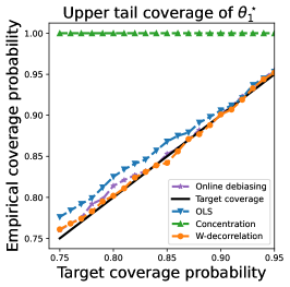
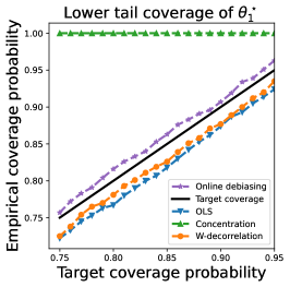
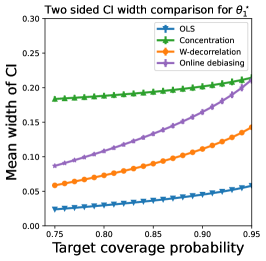
(a) Thompson sampling algorithm

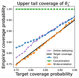
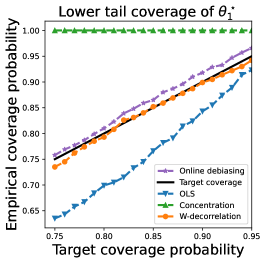
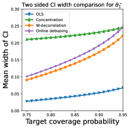
(b) $\varepsilon$-greedy algorithm

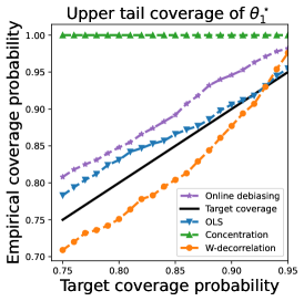
(c) Upper confidence bound (UCB) algorithm

Figure 5: Average coverage and width of confidence intervals for $\theta_{1}^{*}$ across 1000 independent replications of a multi-armed bandit experiment (28) with ${\boldsymbol{\theta}^{*}}\equiv(\theta_{1}^{*},\theta_{2}^{*})=(0.3,0.3)^{\top}$. The covariates $\{\mathbf{x}_{i}\}_{i=1}^{1000}$ were selected using a) Thompson sampling [24], (b) the $\varepsilon$-greedy algorithm [20], and (c) the upper confidence bound algorithm (UCB) [13]. The error bars represent $\pm 1$ standard error. Left and Center: Coverage of one-sided $1-\alpha$ intervals for $\theta_{1}^{*}$. Right: Width of two-sided $1-\alpha$ intervals for $\theta_{1}^{*}$. See Appendix C.1 for details.

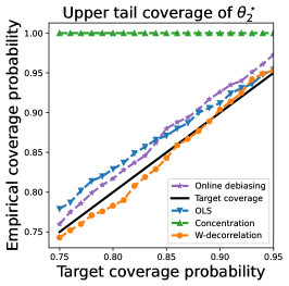
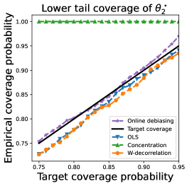
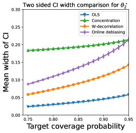
(a) Thompson sampling algorithm

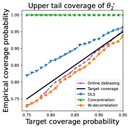
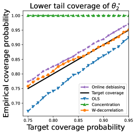
(b) $\varepsilon$-greedy algorithm

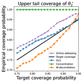
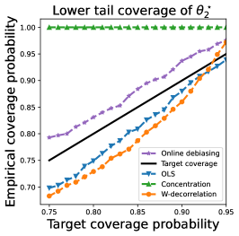
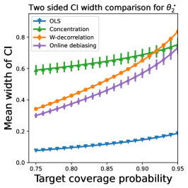
(c) Upper confidence bound (UCB) algorithm

Figure 6: Average coverage and width of confidence intervals for $\theta_{2}^{*}$ across 1000 independent replications of a multi-armed bandit experiment (28) with ${\boldsymbol{\theta}^{*}}\equiv(\theta_{1}^{*},\theta_{2}^{*})=(0.3,0.3)^{\top}$. The covariates $\{\mathbf{x}_{i}\}_{i=1}^{1000}$ were selected using a) Thompson sampling [24], (b) the $\varepsilon$-greedy algorithm [20], and (c) the upper confidence bound algorithm (UCB) [13]. The error bars represent $\pm 1$ standard error. Left and Center: Coverage of one-sided $1-\alpha$ intervals for $\theta_{2}^{*}$. Right: Width of two-sided $1-\alpha$ intervals for $\theta_{2}^{*}$. See Appendix C.1 for details.

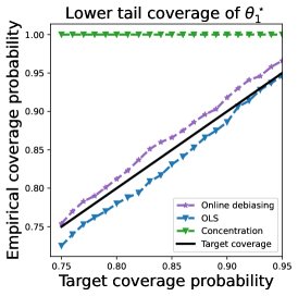
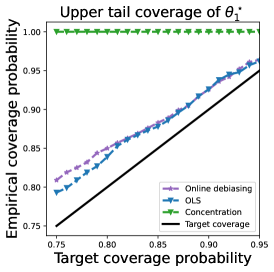
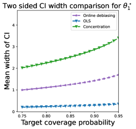
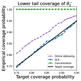
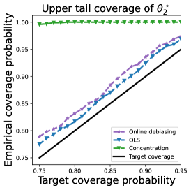
(a) Plots for $\lambda_{\text{ridge}}=1$

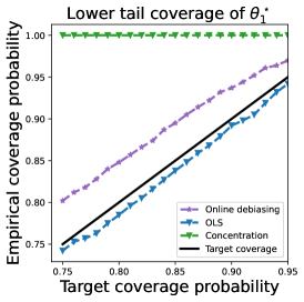
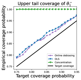
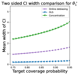
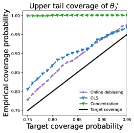
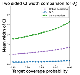
(b) Plots for $\lambda_{\text{ridge}}=10$

Figure 7: Average coverage and width of confidence intervals for $\theta_{1}^{*}$ and $\theta_{2}^{*}$ across 1000 independent replications of linear bandits experiment (39) with ${\boldsymbol{\theta}^{*}}\equiv(\theta_{1}^{*},\theta_{2}^{*})=(0.3,0.3)^{\top}$. The covariates $\{\mathbf{x}_{i}\}_{i=1}^{1000}$ were selected using the $\varepsilon$-greedy linear bandits algorithm (39), and the error bars represent $\pm 1$ standard error. Left and Center: Coverage of one-sided $1-\alpha$ intervals Right: Width of two-sided $1-\alpha$ intervals. See Appendix C.2 for details.

Appendix D Comparison to the least squares estimator

In this section, we provide a more fine-grained comparison between the least squares estimator and the online debiased estimator. We start with a lower bound on the MSE of the ordinary least squares estimator, which is based on the law of iterated logarithm.

Law of the iterated logarithm lower bound

Let $\epsilon_{1},\epsilon_{2},\ldots$ be a sequence of independent standard Gaussian random variables and and $d=1$ and ${\boldsymbol{\theta}^{*}}=0$, which means the least squares estimator is

$$\hat{\theta}_{n}=\frac{\sum_{i=1}^{n}\mathbf{x}_{i}\epsilon_{i}}{\sum_{i=1}^{n}\mathbf{x}_{i}^{2}}\,.$$

We will choose an adaptive design with $\mathbf{x}_{i}\in\{0,1\}$ and for which

$$\limsup_{n\to\infty}\mathbb{P}(\mathcal{E}_{n}>1)\geq\frac{1}{2}\,\,\qquad\text{with}\qquad\mathcal{E}_{n}=\frac{\mathbf{S}_{n}^{1/2}\hat{\theta}_{n}}{\sqrt{\frac{1}{2}\log\log n}}\,.$$

The construction is essentially based on using the adaptive covariates to derandomize the law of the iterated logarithm. Let $M_{t}=\sum_{i=1}^{t}\epsilon_{i}$ be a Gaussian random walk. Define a sequence of intervals $\{m_{k},m_{k}+\ell_{k}-1\}$ of length $\ell_{k}$ inductively as follows. Let $m_{0}=0$ and $m_{k}=m_{k-1}+\ell_{k}$ where

$$\ell_{k}=\min\left\{\ell:\mathbb{P}\Big{(}\text{exists }1\leq s\leq\ell:M_{s}\geq\sqrt{(m_{k-1}+s)\log\log m_{k-1}}\Big{)}\geq\frac{1}{2}\right\}\,.$$

By the same tedious argument used in the proof of the law of the iterated logarithm one can also show that $\log\log m_{k+1}\leq 2\log\log m_{k}$ for suitably large $k$. By symmetry,

$$\mathbb{P}\left(\text{exists }m_{k-1}+1\leq t\leq m_{k-1}+\ell_{k}:|M_{t}|\geq\sqrt{t\log\log m_{k-1}}\Big{|}M_{m_{k-1}}\right)\geq\frac{1}{2}\,\,a.s.\,.$$

Let $\mathbb{N}=\cup_{k=1}^{\infty}I_{k}$ where $\{I_{k}:k\in\mathbb{N}\}$ are disjoint consecutive intervals and $I_{k}$ has length $2\ell_{k}$. We choose an adaptive design so that $\mathbf{x}_{i}\in\{0,1\}$ for all $i$ and $\sum_{i\in I_{k}}\mathbf{x}_{i}=\ell_{k}$ for all $k$. That is, $\mathbf{x}_{i}=1$ in exactly half of the time in each interval. The adaptivity within each interval is as follows. The feature $\mathbf{x}_{i}=1$ for either $\ell_{k}$ time-steps or until ${\widehat{U}}_{i-1}\geq 1$. Then $\mathbf{x}_{i}=0$ until a final block of the interval where $\mathbf{x}_{i}=1$ to guarantee that $\sum_{i\in I_{k}}\mathbf{x}_{i}=\ell_{k}$ holds. Formally,

$$\mathbf{x}_{i} =\begin{cases}0&\text{if }m(i-1)=m_{k}\\ 1&\text{if }\mathcal{E}_{i-1}\leq 1\\ 1&\text{if }m(i-1)+|I_{k}\setminus\{1,2,\ldots,i-1\}|=m_{k}\\ 0&\text{otherwise}\,.\end{cases}$$

By construction, if $s_{k}$ is the $\ell_{k}$th time-step in interval $I_{k}$, then

$$\mathbb{P}\left({\widehat{U}}_{s_{k}}>1\right) =\mathbb{P}\left(\sum_{i=1}^{s_{k}}\mathbf{x}_{i}\epsilon_{i}\geq\sqrt{\frac{m(s_{k})}{2}\log\log s_{k}}\right)$$

$$\geq\mathbb{P}\left(\sum_{i=1}^{s_{k}}\mathbf{x}_{i}\epsilon_{i}\geq\sqrt{m(s_{k})\log\log m_{k-1}}\right)$$

$$\geq\frac{1}{2}\,.$$

Reducing bias via post debiasing correction

In this section, we consider a modified version of the online debiased estimator. Throughout this section, we assume $\operatorname{\mathbb{E}}[\mathbf{\epsilon}_{i}^{2}]=1$. We show that this modified estimator can have less bias for certain multiarmed bandit problems, and thereby improving upon the performance of the least squares estimators. We also show that this improved estimator has the same performnace as online debiased estimator (6) in the worst case. We start with the following modified version of the online debiased estimtor

$$\widehat{\theta}_{OD}=\widehat{\boldsymbol{\theta}}_{\scriptscriptstyle{\operatorname{LS}}}+\sqrt{\frac{\gamma_{n}}{\widehat{\gamma}_{n}}}\cdot\sum_{i=1}^{n}\mathbf{S}_{n}^{-\frac{1}{2}}\mathbf{w}_{i}\left(y_{i}-\mathbf{x}_{i}^{\top}\widehat{\boldsymbol{\theta}}_{\scriptscriptstyle{\operatorname{LS}}}\right)$$ (67)

where

$$\sqrt{\widehat{\gamma}_{n}}=\max\left\{\mathbf{e}_{j}^{\top}\sqrt{\gamma_{n}}\sum_{i=1}^{n}\mathbf{w}_{i}\mathbf{x}_{i}^{\top}\mathbf{S}_{n}^{-\frac{1}{2}}\mathbf{e}_{j}\;,\;\frac{1}{\log(n)\cdot\log\log(n)}\right\}$$ (68)

Focusing on a k-armed bandit problem, we assume that the tuning parameters $\gamma_{n}$, and $\{\mathbf{\Gamma}_{i,n}\}_{i\leq n}$ satisfy the following conditions

$$\gamma_{n}\rightarrow 0,\qquad\text{and}\qquad\frac{\gamma_{n}}{\log(n)\cdot\log\log(n)}\rightarrow\infty.$$ (69a)

$$\frac{1}{\gamma_{n}}\max_{i\in[n]}\cdot\mathbf{x}_{i}^{\top}\Gamma_{i,n}^{-1}\mathbf{x}_{i}\stackrel{{\scriptstyle{\operatorname{p}}}}{{\longrightarrow}}0\qquad\text{and}\qquad\mathbf{S}_{n}\succ\Gamma_{i,n}\succ 0.$$ (69b)

$$\mathbf{e}_{j}^{\top}\mathbf{S}_{n}^{-1}\mathbf{\Gamma}_{i,n}\mathbf{e}_{j}>c_{1}>0\qquad\text{for all}\quad n\geq 1\;\;\text{and}\;\;i\leq n.$$ (69c)

Theorem 3.

Given a target direction $\mathbf{e}_{j}$, suppose the covariance matrix $\mathbf{S}_{n}$ of a $k$-armed bandits problem satisfies conditions (69a), (69b) and (69c). Then the online debiased estimator from (67) satisfies

$$\sqrt{\widehat{\gamma}_{n}}\mathbf{e}_{j}^{\top}\cdot\mathbf{S}^{\frac{1}{2}}(\widehat{\theta}_{OD}-{\boldsymbol{\theta}^{*}})\stackrel{{\scriptstyle{\operatorname{d}}}}{{\longrightarrow}}\mathcal{N}(0,1)\quad\text{and}\quad\lim\sup\sqrt{\frac{\widehat{\gamma}_{n}}{\gamma_{n}}}\geq O_{p}(\sqrt{c_{1}}).$$ (70)

Moreover, we have

$$\operatorname{\mathbb{E}}\left(\sqrt{\widehat{\gamma}_{n}}\mathbf{e}_{j}^{\top}\cdot\mathbf{S}^{\frac{1}{2}}(\widehat{\theta}_{OD}-{\boldsymbol{\theta}^{*}})\right)^{2}=\gamma_{n}\operatorname{\mathbb{E}}\left(\sum_{i=1}^{n}\mathbf{e}_{j}^{\top}\mathbf{w}_{i}\mathbf{w}_{i}^{\top}\mathbf{e}_{j}\right)\leq 1.$$ (71)

See Appendix E for a proof of Theorem 3.

Appendix E Proof of Theorem 3 and related results

In this section, we provide a proof of Theorem 3. We show shortly that under the conditions of Theorem 3

$$\sqrt{\widehat{\gamma}_{n}}=\mathbf{e}_{j}^{\top}\sqrt{\gamma_{n}}\sum_{i=1}^{n}\mathbf{w}_{i}\mathbf{x}_{i}^{\top}\mathbf{S}_{n}^{-\frac{1}{2}}\mathbf{e}_{j}$$ (72)

We come back to the proof of this statement in Lemma 7, but let us complete the proof assuming this cindition is true. A simple calculation using the definition of $\widehat{\gamma}_{n}$ from (68) yields

$$\mathbf{e}_{j}^{\top}\sqrt{\widehat{\gamma}_{n}}\mathbf{e}_{j}^{\top}\cdot\mathbf{S}^{\frac{1}{2}}(\widehat{\theta}_{OD}-{\boldsymbol{\theta}^{*}}) =\mathbf{e}_{j}^{\top}\left(\sqrt{\widehat{\gamma}_{n}}\cdot\mathbf{I}-\sqrt{\gamma_{n}}\sum_{i=1}^{n}\mathbf{w}_{i}\mathbf{x}_{i}^{\top}\mathbf{S}_{n}^{-\frac{1}{2}}\right)\mathbf{S}_{n}^{\frac{1}{2}}(\widehat{\boldsymbol{\theta}}_{\scriptscriptstyle{\operatorname{LS}}}-{\boldsymbol{\theta}^{*}})$$

$$\qquad\qquad+\mathbf{e}_{j}^{\top}\sqrt{\gamma_{n}}\sum_{i=1}^{n}\mathbf{w}_{i}\mathbf{\epsilon}_{i}$$

$$=\mathbf{e}_{j}^{\top}\sqrt{\gamma_{n}}\sum_{i=1}^{n}\mathbf{w}_{i}\mathbf{\epsilon}_{i}.$$

In order to prove asumptotic normality for $\sqrt{\widehat{\gamma}_{n}}\mathbf{e}_{j}^{\top}\cdot\mathbf{S}^{\frac{1}{2}}(\widehat{\theta}_{OD}-{\boldsymbol{\theta}^{*}})$ it now suffices to find weights $\{\mathbf{w}_{i}\}_{i=1}^{n}$ such that the weights are stabilized. Concretely, we require

$$\gamma_{n}\sum_{i=1}^{n}\mathbf{w}_{i}\mathbf{w}_{i}^{\top} \stackrel{{\scriptstyle{\operatorname{p}}}}{{\longrightarrow}}\mathbf{I}$$ (73a)

$$\max_{i\in[n]}\;\;\sqrt{\gamma_{n}}\|\mathbf{w}_{i}\|_{2} \stackrel{{\scriptstyle{\operatorname{p}}}}{{\longrightarrow}}0.$$ (73b)

Putting together the pieces we conclude that for any set tuning parameters $\gamma_{n}$ and $\{\mathbf{w}_{i}\}_{i\geq 1}$ satisfying conditions (73a) and (73b) we have

$$\sqrt{\widehat{\gamma}_{n}}\mathbf{e}_{j}^{\top}\cdot\mathbf{S}^{\frac{1}{2}}(\widehat{\theta}_{OD}-{\boldsymbol{\theta}^{*}})\stackrel{{\scriptstyle{\operatorname{d}}}}{{\longrightarrow}}\mathcal{N}(0,1).$$

The proof of the second part is immediate from the definition of $\widehat{\gamma}_{n}$ and from the fact that $\gamma_{n}\sum_{i=1}^{n}\mathbf{w}_{i}\mathbf{w}_{i}^{\top}=\mathbf{I}-A_{n}-B_{n}$ for appropriate positive semidefinite matrices $A_{n},B_{n}$; see the the decomposition (65) for instance. We prove part (ii) of the claim (70) in Lemma 7. It now remains to derive conditions which guarantee the two properties  (73a) and (73b). Towards this end we prove the following lemma.

Lemma 6.

Suppose the sample covariance matrix $\mathbf{S}_{n}$ of a $k$-armed bandit problem satisfies the condition 69b for some non-random scalars $\gamma_{n}$ and diagonal matrices $\{\Gamma_{i,n}\}_{i,n\geq 1}$. Then conditions (73a) and (73b) are satisfied.

Proof.

Invoking Lemma 1 we see that we only need to verify Assumptions (A3) (a) and (c). Condition (A3) (a) is readily satisfied by the second condition in (69b). To verify condition (A3) (c), invoking Lemma 2 we have

$$|\!|\!|\mathbf{I}_{d}-\sum_{i=1}^{n}\mathbf{w}_{i}\mathbf{x}_{i}^{\top}\mathbf{\Gamma}_{i,n}^{-\frac{1}{2}}|\!|\!|_{{\scriptsize{\operatorname{op}}}} \leq\exp\left(-\frac{\lambda_{\min}(\sum_{i=1}^{n}\mathbf{\Gamma}_{i,n}^{-\frac{1}{2}}\mathbf{x}_{i}\mathbf{x}_{i}^{\top}\mathbf{\Gamma}_{i,n}^{-\frac{1}{2}})}{\gamma_{n}}\right)$$

$$\stackrel{{\scriptstyle(i)}}{{\leq}}\exp\left(-\frac{\lambda_{\min}(\sum_{i=1}^{n}\mathbf{S}_{n}^{-\frac{1}{2}}\mathbf{x}_{i}\mathbf{x}_{i}^{\top}\mathbf{S}_{n}^{-\frac{1}{2}})}{\gamma_{n}}\right)$$

$$=\exp(-1/\gamma_{n})\rightarrow 0.$$

The inequality (i) above follows from the third condition in (69b) and the last deduction follows from the asusmption that $\gamma_{n}\rightarrow 0$. This completes the proof of Lemma 6. ∎

Control on $\widehat{\gamma}_{n}$:

Next we discuss the scaling of $\widehat{\gamma}_{n}$. Note that the scaling of $\widehat{\gamma}_{n}$ controls the asymptotic variance of the online debiased estimator $\widehat{\theta}_{OD}$ from equation (67); smaller values of $\widehat{\gamma}_{n}$ leads to a larger asymptotic variance. The scaling of $\widehat{\gamma}_{n}$ is controlled by the following lemma.

Lemma 7.

Give a target direction $\mathbf{e}_{j}$, suppose the sample covariance matrix $\mathbf{S}_{n}$ of a $k$-armed bandit problem satiafies condition (69c), and assume that the conditios of Lemma 6 are in force. Then the weights $\mathbf{w}_{i}$ produced by any $\gamma_{n}\rightarrow 0$ and scaling matrix $\mathbf{\Gamma}_{i}$ from (69c) ensures

$$\lim\sup\sqrt{\frac{\widehat{\gamma}_{n}}{\gamma_{n}}}\geq O_{p}(\sqrt{c_{1}})$$

Consequently, the condition (72) is satisfied.

Proof.

Invoking the proof of Lemma 2 we know that the matrix $\sum_{i\leq n}\mathbf{w}_{i}\mathbf{x}_{i}^{\top}\mathbf{\Gamma}_{i,n}^{-\frac{1}{2}}$ is diagonal. Furthermore, conditions of Lemma 6 ensures that the condition A3 (c) is satisfied and we have

$$\mathbf{e}_{j}^{\top}\sum_{i\leq n}\mathbf{w}_{i}\mathbf{x}_{i}^{\top}\mathbf{\Gamma}_{i,n}^{-\frac{1}{2}}\stackrel{{\scriptstyle{\operatorname{p}}}}{{\longrightarrow}}\mathbf{e}_{j}^{\top}.$$

Combing the last step with the condition (69c) and the fact that the matrices $\mathbf{\Gamma}_{i,n}$, $\mathbf{S}_{n}$ and $\sum_{i\leq n}\mathbf{w}_{i}\mathbf{x}_{i}^{\top}\mathbf{\Gamma}_{i,n}^{-\frac{1}{2}}$ are diagonal yields

$$\sqrt{\frac{\widehat{\gamma}_{n}}{\gamma_{n}}} =\mathbf{e}_{j}^{\top}\sum_{i=1}^{n}\mathbf{w}_{i}\mathbf{x}_{i}^{\top}\mathbf{S}_{n}^{-\frac{1}{2}}\mathbf{e}_{j}$$

$$=\mathbf{e}_{j}^{\top}\sum_{i=1}^{n}\mathbf{w}_{i}\mathbf{x}_{i}^{\top}\mathbf{\Gamma}_{i,n}^{-\frac{1}{2}}\mathbf{\Gamma}_{i,n}^{\frac{1}{2}}\mathbf{S}_{n}^{-\frac{1}{2}}\mathbf{e}_{j}$$

$$\geq\sqrt{c_{1}}\cdot\mathbf{e}_{j}^{\top}\sum_{i=1}^{n}\mathbf{w}_{i}\mathbf{x}_{i}^{\top}\mathbf{\Gamma}_{i,n}^{-\frac{1}{2}}\mathbf{e}_{j}$$

$$\geq\sqrt{c_{1}}\cdot O_{p}(1).$$

The last line combined with condition (69a) ensures that the condition (72) is satisfied. This completes the proof of Lemma 7. ∎

E.1 Worst case performance:

Next, we consider the choice of $\widehat{\gamma}_{n}$ when the condition (72) is not satisfied. A simple calculation using the fact that the matrices $\mathbf{S}_{n}$ and $\mathbf{w}_{i}\mathbf{x}_{i}^{\top}$ are diagonal for a multiarmed bandit problem, we have

$$\sqrt{\widehat{\gamma}_{n}}\cdot\mathbf{e}_{j}^{\top}\cdot\mathbf{S}^{\frac{1}{2}}(\widehat{\theta}_{OD}-{\boldsymbol{\theta}^{*}}) =\mathbf{e}_{j}^{\top}\cdot\left(\sqrt{\widehat{\gamma}_{n}}\cdot\mathbf{I}-\sqrt{\gamma_{n}}\sum_{i=1}^{n}\mathbf{w}_{i}\mathbf{x}_{i}^{\top}\mathbf{S}_{n}^{-\frac{1}{2}}\right)\mathbf{S}_{n}^{\frac{1}{2}}(\widehat{\boldsymbol{\theta}}_{\scriptscriptstyle{\operatorname{LS}}}-{\boldsymbol{\theta}^{*}})+\sqrt{\gamma_{n}}\sum_{i=1}^{n}\mathbf{w}_{i}\mathbf{\epsilon}_{i}$$

$$=\sqrt{\widehat{\gamma}_{n}}\cdot\mathbf{e}_{j}^{\top}\cdot\mathbf{S}_{n}^{\frac{1}{2}}(\widehat{\boldsymbol{\theta}}_{\scriptscriptstyle{\operatorname{LS}}}-{\boldsymbol{\theta}^{*}})-\sqrt{\gamma_{n}}\mathbf{e}_{j}^{\top}\cdot\sum_{i=1}^{n}\mathbf{w}_{i}\mathbf{x}_{i}^{\top}\mathbf{S}_{n}^{-\frac{1}{2}}\mathbf{e}_{j}\cdot\mathbf{e}_{j}^{\top}\mathbf{S}_{n}^{\frac{1}{2}}(\widehat{\boldsymbol{\theta}}_{\scriptscriptstyle{\operatorname{LS}}}-{\boldsymbol{\theta}^{*}})$$

$$\qquad\qquad+\sqrt{\gamma_{n}}\sum_{i=1}^{n}\mathbf{e}_{j}^{\top}\cdot\mathbf{w}_{i}\mathbf{\epsilon}_{i}$$ (74)

The third term above converges in distribution to $\mathcal{N}(0,1)$ following the arguments in the proof of Theorem 3. The first two terms in the last line correspnds to the bias-term in the modified online debiased estimator, and we show that they converge to zero in probablity. The first term in (74) above can be bounded as

$$\|\sqrt{\widehat{\gamma}_{n}}\cdot\mathbf{S}_{n}^{\frac{1}{2}}(\widehat{\boldsymbol{\theta}}_{\scriptscriptstyle{\operatorname{LS}}}-{\boldsymbol{\theta}^{*}})\|_{2} =\sqrt{\widehat{\gamma}_{n}}\cdot O_{p}(\log(n))$$

$$=o_{p}(1/\sqrt{\log(n)})\cdot O_{p}(\sqrt{\log(n)})=o_{p}(1).$$

Focusing on the second term in (74) and using the fact that condition (72) is violated

$$|\sqrt{\gamma_{n}}\mathbf{e}_{j}^{\top}\cdot\sum_{i=1}^{n}\mathbf{w}_{i}\mathbf{x}_{i}^{\top}\mathbf{S}_{n}^{-\frac{1}{2}}\mathbf{e}_{j}\cdot\mathbf{e}_{j}^{\top}\mathbf{S}_{n}^{\frac{1}{2}}(\widehat{\boldsymbol{\theta}}_{\scriptscriptstyle{\operatorname{LS}}}-{\boldsymbol{\theta}^{*}})|$$

$$\stackrel{{\scriptstyle(i)}}{{\leq}}|\sqrt{\gamma_{n}}\mathbf{e}_{j}^{\top}\cdot\sum_{i=1}^{n}\mathbf{w}_{i}\mathbf{x}_{i}^{\top}\mathbf{S}_{n}^{-\frac{1}{2}}\mathbf{e}_{j}|\cdot|\mathbf{e}_{j}^{\top}\mathbf{S}_{n}^{\frac{1}{2}}(\widehat{\boldsymbol{\theta}}_{\scriptscriptstyle{\operatorname{LS}}}-{\boldsymbol{\theta}^{*}})|$$

$$\leq\frac{1}{\sqrt{\log(n)\cdot\log\log(n)}}\cdot O_{p}(\sqrt{\log(n)})=o_{p}(1).$$

where step (i) utilizes the fact that condition (72) is violated, and hence

$$0\leq\mathbf{e}_{j}^{\top}\sqrt{\gamma_{n}}\sum_{i=1}^{n}\mathbf{w}_{i}\mathbf{x}_{i}^{\top}\mathbf{S}_{n}^{-\frac{1}{2}}\mathbf{e}_{j}\leq\frac{1}{\sqrt{\log(n)\cdot\log\log(n)}}$$

Recall that by construction, in the special case of multi-armed bandits, the matrix $\mathbf{w}_{i}\mathbf{x}_{i}^{\top}$ is a diagonal matrix with non-negative entries.

Putting together the pieces we conclude that for a multiarm bandit problem, under the conditions

$$\gamma_{n}\rightarrow 0\qquad\text{and}\qquad\frac{1}{\gamma_{n}}\max_{i\in[n]}\cdot\mathbf{x}_{i}^{\top}\Gamma_{i,n}^{-1}\mathbf{x}_{i}\stackrel{{\scriptstyle{\operatorname{p}}}}{{\longrightarrow}}0,$$

we have

$$\sqrt{\widehat{\gamma}_{n}}\mathbf{e}_{j}^{\top}\cdot\mathbf{S}^{\frac{1}{2}}(\widehat{\theta}_{OD}-{\boldsymbol{\theta}^{*}})\stackrel{{\scriptstyle{\operatorname{d}}}}{{\longrightarrow}}\mathcal{N}(0,1).$$

Proposition 3.

Assume that the satbility condition 5 is satisfied, $\|\mathbf{x}_{i}\|\leq 1$, and conditions (A1) and (A2) are in force. Then condition (A3) is satisfied with $\gamma_{n}=1$ and $\mathbf{\Gamma}_{i}=B_{n}$.

Proof.

Combining condition (A2) and the stability condition 5 we have $\lambda_{\min}(B_{n})\stackrel{{\scriptstyle{\operatorname{p}}}}{{\longrightarrow}}0$. This combined with $\|\mathbf{x}_{i}\|\leq 1$ensures that part (a) of (A3) is satisfied. Next, under the stability condition 5 and using $\mathbf{w}_{i}=\mathbf{x}_{i}\mathbf{\Gamma}_{i}^{-\frac{1}{2}}=\mathbf{x}_{i}B_{n}^{-\frac{1}{2}}$ we have

$$\mathbf{W}\mathbf{X}\mathbf{S}_{n}^{-\frac{1}{2}}=B_{n}^{-\frac{1}{2}}\sum_{i=1}^{n}\mathbf{x}_{i}\mathbf{x}_{i}^{\top}\mathbf{S}_{n}^{-\frac{1}{2}}=B_{n}^{-\frac{1}{2}}\mathbf{S}_{n}^{\frac{1}{2}}\stackrel{{\scriptstyle{\operatorname{p}}}}{{\longrightarrow}}\mathbf{I}.$$

Observe that the psd matrix $B_{n}$ is is invertible by assumption (A2) and the stability condition 5. This verifies part (b) of assumption (A3). Finally, we note that

$$\sum_{i=1}^{n}\mathbf{w}_{i}\mathbf{x}_{i}\mathbf{\Gamma}_{i}^{-\frac{1}{2}}=B_{n}^{-\frac{1}{2}}\sum_{i=1}^{n}\mathbf{x}_{i}\mathbf{x}_{i}^{\top}B_{n}^{-\frac{1}{2}}=B_{n}^{-\frac{1}{2}}\mathbf{S}_{n}B_{n}^{-\frac{1}{2}}\stackrel{{\scriptstyle{\operatorname{p}}}}{{\longrightarrow}}\mathbf{I}$$

This verifies part (c) of Assumption (A3). ∎

Appendix F Proofs related to Theorem 2 part (b)

In this appendix, we prove the bounds (53a) and (53b) that were used in the proof of part (b) of Theorem 2

Proof of the bound (53a)

Let $v=n/(d-1)$. By Bayes’ rule,

$$\frac{{\widehat{U}}_{n}}{1-{\widehat{U}}_{n}} =\prod_{u=1}^{d-1}\frac{1}{\sqrt{2\pi}}\int_{\mathbb{R}}\exp\left(-\frac{1}{2}\sum_{w=1}^{v}(a_{u,w}+b_{w}\varphi-y_{u,w})^{2}+\frac{1}{2}\sum_{i=1}^{n}y_{u,w}^{2}-\frac{\varphi^{2}}{2}\right)d\varphi$$

$$=\prod_{u=1}^{d-1}\exp\left(\sum_{w=1}^{v}a_{u,w}y_{u,w}-\frac{1}{2}\sum_{w=1}^{v}a_{u,w}^{2}+\frac{m_{u,v}^{2}}{2d_{v}}-\frac{1}{2}\log d_{v}\right)$$

$$:\,=\exp\left(\sum_{u=1}^{d-1}Z_{u,w}\right)\,.$$

Note that ${\widehat{U}}_{n}(1-{\widehat{U}}_{n})=\Omega_{p}(1)$ is equivalent to $|\sum_{u=1}^{d-1}Z_{u,w}|=O_{p}(1)$, which we now establish. To begin,

$$\frac{m_{u,w+1}^{2}}{d_{w+1}} =\frac{m_{u,w}^{2}}{d_{w}}+\frac{a_{u,w+1}^{2}d_{w}}{d_{w+1}}+\frac{b_{w+1}^{2}(y_{u,w+1}-a_{u,w+1})^{2}}{d_{w+1}}-\frac{2a_{u,w+1}d_{w}}{d_{w+1}}y_{u,w+1}\,.$$

Telescoping shows that

$$Z_{u,v}=\underbracket{-\frac{1}{2}\sum_{w=1}^{v}\frac{b_{w}^{2}a_{u,w}^{2}}{d_{w}}}_{\textrm{A}_{u,v}}+\underbracket{\sum_{w=1}^{v}\frac{b_{w}^{2}a_{u,w}y_{u,w}}{d_{w}}}_{\textrm{B}_{u,v}}+\underbracket{\frac{1}{2}\sum_{w=1}^{v}\frac{b_{w}^{2}(y_{u,w}-a_{u,w})^{2}}{d_{w}}-\frac{1}{2}\log d_{v}}_{\textrm{C}_{u,v}}\,.$$

By definition, $b_{w}=w^{-1/4}/d^{1/2}$ and $d_{w}=\Omega(w^{1/2}/d)$. Furthermore,

$${\operatorname{\mathbb{E}}}[a_{u,w}^{2}]=b_{w}^{2}\left(\left(\frac{d_{w-1}-1}{d_{w-1}}\right)^{2}+\frac{d_{w-1}-1}{d_{w-1}^{2}}\right)=O(b_{w}^{2})\text{ and }{\operatorname{\mathbb{E}}}[y_{u,w}^{2}]=O(1)\,.$$

Therefore, by Cauchy-Schwarz and Chebyshev’s inequality, $|\sum_{u=1}^{d-1}\textrm{A}_{u,v}|=O_{p}(1)$ and $|\sum_{u=1}^{d-1}\textrm{B}_{u,v}|=O_{p}(1)$ and

$$\left|\sum_{u=1}^{d-1}\textrm{C}_{u,v}\right| =\frac{1}{2}\left|\sum_{u=1}^{d-1}\sum_{w=1}^{v}\frac{b_{w}^{2}(y_{u,w}-a_{u,w})^{2}}{d_{w}}-\log d_{v}\right|$$

$$=\frac{1}{2}\left|\sum_{u=1}^{d-1}\sum_{w=1}^{v}\frac{b_{w}^{2}(b_{w}+\mathbf{\epsilon}_{u,w})^{2}}{d_{w}}-\log d_{v}\right|$$

$$=\frac{1}{2}\left|\sum_{u=1}^{d-1}\sum_{w=1}^{v}\frac{b_{w}^{4}+b_{w}^{2}\mathbf{\epsilon}_{u,w}^{2}+2b_{w}^{3}\mathbf{\epsilon}_{u,w}}{d_{w}}-\log d_{v}\right|$$

$$=\frac{1}{2}\left|\sum_{u=1}^{d-1}\sum_{w=1}^{v}\frac{b_{w}^{2}}{d_{w}}-\log d_{v}\right|+O_{p}(1)$$

$$=O_{p}(1)\,,$$

where the second last equality follows from Chebyshev’s inequality and the last by an elementary integral approximation. Therefore $|\sum_{u=1}^{d-1}Z_{u,v}|=O_{p}(1)$, which completes the proof of (53a).

Proof of bound 53b

By definition,

$$\mathbf{S}_{n}=\left[\begin{matrix}\sum_{w=1}^{v}b_{w}^{2}&0&\cdots&\sum_{w=1}^{v}a_{1,w}b_{w}\\ 0&\ddots&0&\vdots\\ \vdots&0&\sum_{w=1}^{v}b_{w}^{2}&\sum_{w=1}^{v}a_{d-1,w}b_{w}\\ \sum_{w=1}^{v}a_{1,w}b_{w}&\cdots&\sum_{w=1}^{v}a_{d-1,w}b_{w}&\sum_{u=1}^{d-1}\sum_{w=1}^{v}a_{u,v}^{2}\end{matrix}\right]$$

Using the formula for the inverse of a block matrix,

$$1/\|e_{d}\|^{2}_{\mathbf{S}_{n}^{-1}} =1/(\mathbf{S}_{n}^{-1})_{d,d}$$

$$=\sum_{u=1}^{d-1}\sum_{w=1}^{v}a_{u,w}^{2}-\sum_{u=1}^{d-1}\frac{\left(\sum_{w=1}^{v}a_{u,w}b_{w}\right)^{2}}{\sum_{w=1}^{v}b_{w}^{2}}$$

$$=\sum_{u=1}^{d-1}\sum_{w=1}^{v}b_{w}^{2}\left(\theta^{*}_{u}+a_{u,w}/b_{w}\right)^{2}-\sum_{u=1}^{d-1}\left(\frac{\sum_{w=1}^{v}b_{w}^{2}(\theta^{*}_{u}+a_{u,w}/b_{u,w})}{\sqrt{\sum_{i=1}^{n}b_{w}^{2}}}\right)^{2}\,.$$ (75)

By the definition of $a_{u,w}$,

$$\theta^{*}_{u}+\frac{a_{u,w}}{b_{w}}=\frac{\theta^{*}_{u}-\sum_{s=1}^{w-1}b_{s}\mathbf{\epsilon}_{u,s}}{d_{w-1}}\,.$$

Therefore,

$$\sum_{u=1}^{d-1}\sum_{w=1}^{v}b_{w}^{2}(\theta^{*}_{u}+a_{u,w}/b_{w})^{2} =\sum_{u=1}^{d-1}\sum_{w=1}^{v}\frac{b_{w}^{2}}{d_{w-1}^{2}}\left(\theta^{*}_{u}-\sum_{s=1}^{w-1}b_{s}\epsilon_{u,s}\right)^{2}$$

$$\geq\sum_{u=1}^{d-1}\sum_{w=1}^{v}\frac{b_{w}^{2}}{d_{w-1}^{2}}\left(\sum_{s=1}^{w-1}b_{s}\epsilon_{u,s}\right)^{2}-2\sum_{u=1}^{d-1}\theta^{*}_{u}\sum_{w=1}^{v}\frac{b_{w}^{2}}{d_{w-1}^{2}}\sum_{s=1}^{w-1}b_{s}\epsilon_{u,s}$$

$$=\sum_{u=1}^{d-1}\sum_{w=1}^{v}\frac{b_{w}^{2}}{d_{w-1}^{2}}\left(\sum_{s=1}^{w-1}b_{s}\epsilon_{u,s}\right)^{2}-2\sum_{u=1}^{d-1}\theta^{*}_{u}\sum_{s=1}^{v-1}b_{s}\epsilon_{u,s}\sum_{w=s+1}^{v}\frac{b_{w}^{2}}{d_{w-1}^{2}}$$

$$\geq\sum_{u=1}^{d-1}\sum_{w=1}^{v}\frac{b_{w}^{2}}{d_{w-1}^{2}}\left(\sum_{s=1}^{w-1}b_{s}\epsilon_{u,s}\right)^{2}-O_{p}(d)\,,$$ (76)

where the final inequality follows because $\theta^{*}_{2}$ is distributed like a standard Gaussian and

$$\sum_{u=1}^{d-1}\sum_{s=1}^{v-1}b_{s}\epsilon_{u,s}\sum_{w=s+1}^{n}\frac{b_{w}^{2}}{d_{w-1}^{2}} \stackrel{{\scriptstyle d}}{{=}}\mathcal{N}\left(0,\beta^{2}\right)\,, \beta^{2} =\sum_{u=1}^{d-1}\sum_{s=1}^{v-1}b_{s}^{2}\left(\sum_{w=s+1}^{n}\frac{b_{w}^{2}}{d_{w-1}^{2}}\right)^{2}=O(d)\,.$$ (77)

The last calculation needed to lower bound the first term in equation 75 is to bound the sum in equation 76:

$$\sum_{u=1}^{d-1}\sum_{w=1}^{v}\frac{b_{w}^{2}}{d_{w-1}^{2}}\left(\sum_{s=1}^{w-1}b_{s}\epsilon_{u,s}\right)^{2} =\sum_{u=1}^{d-1}\sum_{w=1}^{v-1}\sum_{s=1}^{n-1}\epsilon_{u,w}\epsilon_{u,s}A_{w,s}\,,$$ (78)

where

$$A_{w,s}=b_{w}b_{s}\sum_{t=\max(w,s)+1}^{v}\frac{b_{t}^{2}}{d_{t-1}^{2}}\,.$$

Viewing $A$ as an $(n-1)\times(n-1)$ matrix, the expression in equation 78 is a sum of Gaussian chaos’. A simple calculation using the facts that $b_{i}=i^{-1/4}/\sqrt{d}$ and $d_{i-1}^{2}=\Omega(i/d^{2})$ shows that

$$\operatorname{trace}(A) =\Omega(\log(v/d^{2})) \|A\|_{F} =O(\sqrt{\log(v)})\,.$$

where $\|A\|_{F}$ is Frobenius norm of matrix $A$. By the Hansen–Write inequality [25, Theorem 6.2.1],

$${\operatorname{\mathbb{E}}}\left[\sum_{w=1}^{v-1}\sum_{s=1}^{v-1}\epsilon_{u,w}\epsilon_{u,s}A_{w,s}\right] =\operatorname{trace}(A_{w,s})=\Omega(\log(v/d^{2}))$$

$$\mathbf{V}\left[\sum_{w=1}^{v-1}\sum_{s=1}^{v-1}\epsilon_{u,w}\epsilon_{u,s}A_{w,s}\right] =O(\|A\|_{F}^{2})=O(\log(v))\,.$$

Therefore, by Chebyshev’s inequality, the right-hand side of equation 78 is $\Omega_{P}(d\log(v/d^{2}))$. Moving to the second term in equation 75,

$$\sum_{u=1}^{d-1}\left(\frac{\sum_{w=1}^{v}b_{w}^{2}(\theta^{*}_{u}+a_{u,w}/b_{w})}{\sqrt{\sum_{w=1}^{v}b_{w}^{2}}}\right)^{2} =\sum_{u=1}^{d-1}\left(\frac{\sum_{w=1}^{v}\frac{b_{w}^{2}}{d_{w-1}}\left(\theta^{*}_{u}-\sum_{s=1}^{w-1}b_{s}\mathbf{\epsilon}_{u,s}\right)}{\sqrt{\sum_{w=1}^{v}b_{w}^{2}}}\right)^{2}$$

$$\leq\frac{2\sum_{u=1}^{d-1}(\theta_{u}^{*})^{2}\left(\sum_{w=1}^{v}\frac{b_{w}^{2}}{d_{w-1}}\right)^{2}+2\left(\sum_{w=1}^{v}\frac{b_{w}^{2}}{d_{w-1}}\sum_{s=1}^{w-1}b_{s}\epsilon_{u,s}\right)^{2}}{\sum_{w=1}^{v}b_{w}^{2}}$$

$$=O_{p}(d)\,,$$

where in the final inequality we used the fact that $\theta^{*}_{u}$ is distributed like a standard Gaussian for $u\in\{1,\ldots,d-1\}$ and $(\sum_{w=1}^{v}b_{w}^{2}/d_{w-1})^{2}/(\sum_{w=1}^{v}b_{w}^{2})=O(1)$ to bound the first term while the second term was bounded using the same calculation as in equation 77. Therefore

$$1/\|e_{d}\|^{2}_{\mathbf{S}_{n}^{-1}}=\Omega_{P}\left(\log(v/d^{2})\right)=\Omega_{P}\left(\log(n/d^{3})\right)\,.$$

which completes the proof of equation 53b.

References

• Åström [2012] {bbook}[author] \bauthor\bsnmÅström, \bfnmKarl J\binitsK. J. (\byear2012). \btitleIntroduction to stochastic control theory. \bpublisherCourier Corporation. \endbibitem
• Abbasi-Yadkori, Pál and Szepesvári [2011] {barticle}[author] \bauthor\bsnmAbbasi-Yadkori, \bfnmYasin\binitsY., \bauthor\bsnmPál, \bfnmDavid\binitsD. and \bauthor\bsnmSzepesvári, \bfnmCsaba\binitsC. (\byear2011). \btitleOnline least squares estimation with self-normalized processes: An application to bandit problems. \bjournalarXiv preprint arXiv:1102.2670. \endbibitem
• Boucheron, Lugosi and Massart [2013] {bbook}[author] \bauthor\bsnmBoucheron, \bfnmS.\binitsS., \bauthor\bsnmLugosi, \bfnmG.\binitsG. and \bauthor\bsnmMassart, \bfnmP.\binitsP. (\byear2013). \btitleConcentration inequalities: A nonasymptotic theory of independence. \bpublisherOxford University Press, \baddressOxford, UK. \endbibitem
• Box et al. [2015] {bbook}[author] \bauthor\bsnmBox, \bfnmGeorge EP\binitsG. E., \bauthor\bsnmJenkins, \bfnmGwilym M\binitsG. M., \bauthor\bsnmReinsel, \bfnmGregory C\binitsG. C. and \bauthor\bsnmLjung, \bfnmGreta M\binitsG. M. (\byear2015). \btitleTime series analysis: forecasting and control. \bpublisherJohn Wiley & Sons. \endbibitem
• Deshpande, Javanmard and Mehrabi [2019] {barticle}[author] \bauthor\bsnmDeshpande, \bfnmYash\binitsY., \bauthor\bsnmJavanmard, \bfnmAdel\binitsA. and \bauthor\bsnmMehrabi, \bfnmMohammad\binitsM. (\byear2019). \btitleOnline debiasing for adaptively collected high-dimensional data. \bjournalarXiv preprint arXiv:1911.01040. \endbibitem
• Deshpande et al. [2018] {binproceedings}[author] \bauthor\bsnmDeshpande, \bfnmYash\binitsY., \bauthor\bsnmMackey, \bfnmLester\binitsL., \bauthor\bsnmSyrgkanis, \bfnmVasilis\binitsV. and \bauthor\bsnmTaddy, \bfnmMatt\binitsM. (\byear2018). \btitleAccurate Inference for Adaptive Linear Models. In \bbooktitleInternational Conference on Machine Learning \bvolume35 \bpages1194–1203. \endbibitem
• Dickey and Fuller [1979] {barticle}[author] \bauthor\bsnmDickey, \bfnmDavid A\binitsD. A. and \bauthor\bsnmFuller, \bfnmWayne A\binitsW. A. (\byear1979). \btitleDistribution of the estimators for autoregressive time series with a unit root. \bjournalJournal of the American statistical association \bvolume74 \bpages427–431. \endbibitem
• Dvoretzky et al. [1972] {binproceedings}[author] \bauthor\bsnmDvoretzky, \bfnmAryeh\binitsA. \betalet al. (\byear1972). \btitleAsymptotic normality for sums of dependent random variables. In \bbooktitleProceedings of the Sixth Berkeley Symposium on Mathematical Statistics and Probability, Volume 2: Probability Theory. \bpublisherThe Regents of the University of California. \endbibitem
• Fontaine et al. [2019] {barticle}[author] \bauthor\bsnmFontaine, \bfnmXavier\binitsX., \bauthor\bsnmPerrault, \bfnmPierre\binitsP., \bauthor\bsnmValko, \bfnmMichal\binitsM. and \bauthor\bsnmPerchet, \bfnmVianney\binitsV. (\byear2019). \btitleOnline A-Optimal Design and Active Linear Regression. \bjournalarXiv preprint arXiv:1906.08509. \endbibitem
• Goodwin and Payne [1977] {bbook}[author] \bauthor\bsnmGoodwin, \bfnmGC\binitsG. and \bauthor\bsnmPayne, \bfnmRL\binitsR. (\byear1977). \btitleDynamic system identification experiment design and data analysis. \bseriesMathematics in Science and Engineering, Volume 136. \bpublisherElsevier. \endbibitem
• Hadad et al. [2019] {barticle}[author] \bauthor\bsnmHadad, \bfnmVitor\binitsV., \bauthor\bsnmHirshberg, \bfnmDavid A\binitsD. A., \bauthor\bsnmZhan, \bfnmRuohan\binitsR., \bauthor\bsnmWager, \bfnmStefan\binitsS. and \bauthor\bsnmAthey, \bfnmSusan\binitsS. (\byear2019). \btitleConfidence intervals for policy evaluation in adaptive experiments. \bjournalarXiv preprint arXiv:1911.02768. \endbibitem
• [12] {barticle}[author] \bauthor\bsnmHoward, \bfnmSteven R\binitsS. R., \bauthor\bsnmRamdas, \bfnmAaditya\binitsA., \bauthor\bsnmMcAuliffe, \bfnmJon\binitsJ. and \bauthor\bsnmSekhon, \bfnmJasjeet\binitsJ. \btitleTime-uniform, nonparametric, non-asymptotic confidence sequences. \bjournalThe Annals of Statistics \bpagesTo appear. \endbibitem
• Jamieson et al. [2014] {binproceedings}[author] \bauthor\bsnmJamieson, \bfnmKevin\binitsK., \bauthor\bsnmMalloy, \bfnmMatthew\binitsM., \bauthor\bsnmNowak, \bfnmRobert\binitsR. and \bauthor\bsnmBubeck, \bfnmSébastien\binitsS. (\byear2014). \btitlelil’ucb: An optimal exploration algorithm for multi-armed bandits. In \bbooktitleConference on Learning Theory \bvolume27 \bpages423–439. \endbibitem
• Kaufmann and Koolen [2018] {barticle}[author] \bauthor\bsnmKaufmann, \bfnmEmilie\binitsE. and \bauthor\bsnmKoolen, \bfnmWouter\binitsW. (\byear2018). \btitleMixture martingales revisited with applications to sequential tests and confidence intervals. \bjournalarXiv preprint arXiv:1811.11419. \endbibitem
• Lai [1994] {barticle}[author] \bauthor\bsnmLai, \bfnmTze Leung\binitsT. L. (\byear1994). \btitleAsymptotic properties of nonlinear least squares estimates in stochastic regression models. \bjournalThe Annals of Statistics \bvolume22 \bpages1917–1930. \endbibitem
• Lai and Robbins [1979] {barticle}[author] \bauthor\bsnmLai, \bfnmT L\binitsT. L. and \bauthor\bsnmRobbins, \bfnmHerbert\binitsH. (\byear1979). \btitleAdaptive design and stochastic approximation. \bjournalThe Annals of Statistics \bvolume7 \bpages1196–1221. \endbibitem
• Lai, Robbins and Wei [1979] {barticle}[author] \bauthor\bsnmLai, \bfnmT L_etc\binitsT. L., \bauthor\bsnmRobbins, \bfnmHerbert\binitsH. and \bauthor\bsnmWei, \bfnmC Zi\binitsC. Z. (\byear1979). \btitleStrong consistency of least squares estimates in multiple regression II. \bjournalJournal of Multivariate Analysis \bvolume9 \bpages343–361. \endbibitem
• Lai and Wei [1982] {barticle}[author] \bauthor\bsnmLai, \bfnmTze Leung\binitsT. L. and \bauthor\bsnmWei, \bfnmChing Zong\binitsC. Z. (\byear1982). \btitleLeast squares estimates in stochastic regression models with applications to identification and control of dynamic systems. \bjournalThe Annals of Statistics \bvolume10 \bpages154–166. \endbibitem
• Lattimore [2023] {barticle}[author] \bauthor\bsnmLattimore, \bfnmT.\binitsT. (\byear2023). \btitleA Lower Bound for Linear and Kernel Regression with Adaptive Covariates. \bjournalarXiv. \endbibitem
• Lattimore and Szepesvári [2020] {bbook}[author] \bauthor\bsnmLattimore, \bfnmTor\binitsT. and \bauthor\bsnmSzepesvári, \bfnmCsaba\binitsC. (\byear2020). \btitleBandit algorithms. \bpublisherCambridge University Press. \endbibitem
• Nie et al. [2018] {binproceedings}[author] \bauthor\bsnmNie, \bfnmXinkun\binitsX., \bauthor\bsnmTian, \bfnmXiaoying\binitsX., \bauthor\bsnmTaylor, \bfnmJonathan\binitsJ. and \bauthor\bsnmZou, \bfnmJames\binitsJ. (\byear2018). \btitleWhy adaptively collected data have negative bias and how to correct for it. In \bbooktitleInternational Conference on Artificial Intelligence and Statistics \bvolume84 \bpages1261–1269. \endbibitem
• Shin, Ramdas and Rinaldo [2019a] {binproceedings}[author] \bauthor\bsnmShin, \bfnmJaehyeok\binitsJ., \bauthor\bsnmRamdas, \bfnmAaditya\binitsA. and \bauthor\bsnmRinaldo, \bfnmAlessandro\binitsA. (\byear2019a). \btitleAre sample means in multi-armed bandits positively or negatively biased? In \bbooktitleAdvances in Neural Information Processing Systems \bvolume32 \bpages7102–7111. \endbibitem
• Shin, Ramdas and Rinaldo [2019b] {barticle}[author] \bauthor\bsnmShin, \bfnmJaehyeok\binitsJ., \bauthor\bsnmRamdas, \bfnmAaditya\binitsA. and \bauthor\bsnmRinaldo, \bfnmAlessandro\binitsA. (\byear2019b). \btitleOn the bias, risk and consistency of sample means in multi-armed bandits. \bjournalarXiv preprint arXiv:1902.00746. \endbibitem
• Thompson [1933] {barticle}[author] \bauthor\bsnmThompson, \bfnmWilliam R\binitsW. R. (\byear1933). \btitleOn the likelihood that one unknown probability exceeds another in view of the evidence of two samples. \bjournalBiometrika \bvolume25 \bpages285–294. \endbibitem
• Vershynin [2018] {bbook}[author] \bauthor\bsnmVershynin, \bfnmRoman\binitsR. (\byear2018). \btitleHigh-dimensional probability: An introduction with applications in data science \bvolume47. \bpublisherCambridge university press. \endbibitem
• Villar, Bowden and Wason [2015] {barticle}[author] \bauthor\bsnmVillar, \bfnmSofía S\binitsS. S., \bauthor\bsnmBowden, \bfnmJack\binitsJ. and \bauthor\bsnmWason, \bfnmJames\binitsJ. (\byear2015). \btitleMulti-armed bandit models for the optimal design of clinical trials: benefits and challenges. \bjournalStatistical science: a review journal of the Institute of Mathematical Statistics \bvolume30 \bpages199. \endbibitem
• Wainwright [2019] {bbook}[author] \bauthor\bsnmWainwright, \bfnmMartin J\binitsM. J. (\byear2019). \btitleHigh-dimensional statistics: A non-asymptotic viewpoint. \bpublisherCambridge University Press. \endbibitem
• White [1958] {barticle}[author] \bauthor\bsnmWhite, \bfnmJohn S\binitsJ. S. (\byear1958). \btitleThe limiting distribution of the serial correlation coefficient in the explosive case. \bjournalThe Annals of Mathematical Statistics \bpages1188–1197. \endbibitem
• Xu, Qin and Liu [2013] {binproceedings}[author] \bauthor\bsnmXu, \bfnmMin\binitsM., \bauthor\bsnmQin, \bfnmTao\binitsT. and \bauthor\bsnmLiu, \bfnmTie-Yan\binitsT.-Y. (\byear2013). \btitleEstimation bias in multi-armed bandit algorithms for search advertising. In \bbooktitleAdvances in Neural Information Processing Systems \bvolume26 \bpages2400–2408. \endbibitem
• Zhang, Janson and Murphy [2020] {barticle}[author] \bauthor\bsnmZhang, \bfnmKelly W\binitsK. W., \bauthor\bsnmJanson, \bfnmLucas\binitsL. and \bauthor\bsnmMurphy, \bfnmSusan A\binitsS. A. (\byear2020). \btitleInference for Batched Bandits. \bjournalarXiv preprint arXiv:2002.03217. \endbibitem
• [31] {barticle}[author] \bauthor\bsnmZhang, \bfnmKelly W\binitsK. W., \bauthor\bsnmJanson, \bfnmLucas\binitsL. and \bauthor\bsnmMurphy, \bfnmSusan A\binitsS. A. \btitleStatistical Inference with M-Estimators on Adaptively Collected Data. \endbibitem