Sufficient principal component regression for pattern discovery in transcriptomic data

Abstract

Motivation: Methods for global measurement of transcript abundance such as microarrays and RNA-Seq generate datasets in which the number of measured features far exceeds the number of observations. Extracting biologically meaningful and experimentally tractable insights from such data therefore requires high-dimensional prediction. Existing sparse linear approaches to this challenge have been stunningly successful, but some important issues remain. These methods can fail to select the correct features, predict poorly relative to non-sparse alternatives, or ignore any unknown grouping structures for the features.

Results: We propose a method called SuffPCR that yields improved predictions in high-dimensional tasks including regression and classification, especially in the typical context of omics with correlated features. SuffPCR first estimates sparse principal components and then estimates a linear model on the recovered subspace. Because the estimated subspace is sparse in the features, the resulting predictions will depend on only a small subset of genes. SuffPCR works well on a variety of simulated and experimental transcriptomic data, performing nearly optimally when the model assumptions are satisfied. We also demonstrate near-optimal theoretical guarantees.

Key words: Algorithms; Feature selection; Prediction; Classification

Availability: Code and raw data are freely available at https://github.com/dajmcdon/suffpcr. Package documentation may be viewed at https://dajmcdon.github.io/suffpcr.

Contact: daniel@stat.ubc.ca

1 Introduction

Global transcriptome measurement with microarrays and RNA-Seq is a staple approach in many areas of biological research and has yielded numerous insights into gene regulation. Given data from such experiments, it is often desirable to identify a small number of transcripts whose expression levels are associated with a phenotype of interest (for instance, disease-free survival of cancer patients). Indeed, projects such as The Cancer Genome Atlas (TCGA) have aimed to generate massive volumes of such data to enable molecular characterization of various cancers. While these data are readily available, their high-dimensional nature (tens of thousands of transcript measurements from a single experiment) makes identification of a compact gene expression signature statistically and computationally challenging. While the identification of a minimal gene expression signature is valuable in evaluating disease prognosis, it is also helpful for guiding experimental exploration. In practical terms, a set of five genes highly associated with a certain disease phenotype can be characterized more rapidly, at lower cost, and in more depth than a set of 50 or 100 such genes using genetic techniques such as CRISPR knockout and cancer biological methods such as xenotransplantation of genetically-modified cells into mice. Therefore, this paper prioritizes selecting a small subset of transcript measurements which still provide accurate prediction of phenotypes.

With these goals in mind, supervised linear regression techniques such as ridge regression [22], the lasso [42], elastic net [50], or other penalized methods are often employed. More commonly, especially in genomics applications, the outcomes of interest tend to be the result of groups of genes, which perhaps together describe more complicated processes. Therefore, researchers often turn to unsupervised methods such as principal component analysis (PCA), principal component regression (PCR), and partial least squares (PLS) for both preprocessing and as predictive models [e.g., 7, 17, 26, 43].

In genomics, one may collect expression measurements for thousands of genes from microarrays or RNA-Seq with the goal of predicting phenotypes or class outcomes. In these settings, the number of patients is much smaller than the number of gene measurements, and researchers are interested in (1) the accurate prediction of the phenotype, (2) the correct identification of a handful of predictive genes, and (3) computational tractability. Among these properties, the correct identification of a small number of predictive genes is of crucial importance in practice, since it can lead biologists to further investigate specific genes through CRISPR knockout or other techniques. It is this genetic pattern discovery for which our proposed methodology is intended: data with many more measurements than observations; the potential that some of the measurements may be grouped or correlated; the existence of either a continuous or discrete outcome we wish to predict; and the belief that these predictions only depend on some small collection of groups rather than the entire set of measurements.

1.1 Recent related work

PCA has two main drawbacks when used in high dimensions. The first is that PCA is non-sparse, so it uses information from all the available genes instead of selecting only those which are important, a key objective in omics applications. That is, the right singular vectors or “eigengenes” [1] depend on all the genes measured rather than a small collection. The second is that these sample principal components are not consistent estimators of the population parameters in high dimensions [25]. This means essentially that when the number of patients is smaller than the number of genes, even if the first eigengene could perfectly explain the data, PCA will not be able to recover it.

Modern approaches specifically for pattern discovery in the genomics context such as supervised gene shaving [19], tree harvesting [20], and supervised principal components (SPC) [4, 5, 38] seek to combine the presence of the phenotype with the structure estimation properties of eigendecompositions on the gene expression measurements using unsupervised techniques to obtain the best of both. PLS is common in genomics [8, 28, e.g.], though it remains uncommon in statistics and machine learning, and its theoretical properties are poorly understood. Other recent PCA-based approaches for genetics, though not directly applicable for prediction are SMSSVD [21] and ESPCA [35].

1.2 Contributions

In this paper, we leverage the strong theoretical properties associated with sparse PCA to improve predictive accuracy for regression and classification problems in genomics. We avoid the strong assumptions necessary for SPC, the current state-of-the-art, while obtaining the benefits associated with sparse subspace estimation. In the case that the phenotype is actually generated as a linear function of a handful of genes, our method, SuffPCR, performs nearly optimally: it does as well as if we had known which genes were relevant beforehand. Furthermore, we justify theoretically that our procedure can both predict accurately and recover the correct genes. Our contributions can be succinctly summarized as follows:

1. We present a methodology for discovering small sets of predictive genes using sparse PCA;

2. Our method improves the computational properties of existing sparse subspace estimation approaches to enable previously impossible inference when the number of genes is very large;

3. We demonstrate state-of-the-art performance of our method in synthetic examples and with standard cancer microarray measurements;

4. We provide near-optimal theoretical guarantees.

Our methodology can be used in a variety of genomic pattern discovery settings. One such example is a modified version of traditional differential expression analysis. If we have treatment and control measurements, the logistic version of our method is appropriate with the advantage that it examines the impact of one gene adjusted for the contributions of others. Additionally, with a continuous treatment, the detection power can be increased relative to using an artificial dichotomization.

In Section 2, we motivate the desire for sufficient PCR relative to previous approaches and present details of SuffPCR. Section 3 illustrates performance in simulated, semi-simulated, and real examples and discusses the biological implications of our methods for a selection of cancers. Section 4 gives theoretically justifies our methods, providing guarantees for prediction accuracy and correct gene selection. Section 5 concludes.

Notation.

We use bold uppercase letters to denote matrices, lowercase Arabic letters to denote row vectors and scalars, and uppercase Arabic letters for for random variables. Let $Y$ be a random, real-valued $n$-vector of independent variables $Y_{i}$, and $\mathbf{X}$ be the rowwise concatenation of i.i.d. draws $X_{i}$ from a distribution on $\mathbb{R}^{p}$ with covariance $\bm{\Sigma}$. We denote the observed realization of the outcome variable $Y$ as $y\in\mathbb{R}^{n}$. To be explicit in the genomics context, $\mathbf{X}$ is an $n\times p$ matrix where each row is a set of transcriptomic measurements from RNA-Seq or microarrays for a patient while $y_{i}$ is an observed phenotype of interest for the $i^{\textrm{th}}$ patient. Because $\mathbf{X}$ is a matrix, this symbol represents both a random matrix and its realization. In the following, the meaning should be clear from the context. We assume, without loss of generality, that $\mathbb{E}\left[X_{i}\right]=0$, and that the measurements $\mathbf{X}$ has been centred. The singular value decomposition (SVD) of a matrix $\mathbf{A}$ is $\mathbf{A}=\mathbf{U}(\mathbf{A})\bm{\Lambda}(\mathbf{A})\mathbf{V}^{\mathsf{T}}(\mathbf{A})$. In the specific case of $\mathbf{X}$, we suppress the dependence on $\mathbf{X}$ in the notation and write $\mathbf{X}=\mathbf{U}\bm{\Lambda}\mathbf{V}^{\mathsf{T}}$. We write $\mathbf{A}_{d}$ to indicate the first $d$ columns of the matrix $\mathbf{A}$ and $a_{j}$ to denote the $j^{th}$ row. In the case of the identity matrix, we use a subscript to denote its dimension when necessary: $\mathbf{I}_{p}$. Let $\mbox{tr}(\mathbf{A})$ denote the sum of the diagonal entries of $\mathbf{A}$ while $\lVert\mathbf{A}\rVert_{F}^{2}=\sum_{ij}a_{ij}^{2}$ is the squared Frobenius norm of $\mathbf{A}$. $\lVert\mathbf{A}\rVert_{2,0}$ denotes $(2,0)$-norm of $\mathbf{A}$, that is the number of rows in $\mathbf{A}$ that have non-zero $\ell_{2}$ norm. $\lVert\mathbf{A}\rVert_{1,1}$ is the sum of the row-wise $\ell_{1}$-norms. Finally, $\mathbf{1}(a)$ is the indicator function for the expression $a$, taking value 1 if $a$ is true or 0 if not.

2 Motivation and methodology

Supervised Principal Components [4, 5, 38] is widely used for solving high-dimensional prediction and feature selection problems. It targets dimension reduction and sparsity simultaneously by first screening genes (or individual mRNA probes) based on their marginal correlation with the phenotype (or likelihood ratio test in the case of non-Gaussian noise). Then, it performs PCA on this selected subset and regresses the phenotype on the resulting components (possibly with additional penalization). This procedure is computationally simple, but, zero population marginal correlation is neither necessary nor sufficient to guarantee that the associated population regression coefficient is zero. To make this statement mathematically precise, consider the linear model $Y_{i}=X_{i}^{\mathsf{T}}\beta^{*}+\epsilon_{i},$ where $Y_{i}$ is a real-valued scalar phenotype, $X_{i}$ is real-valued vector of genes, $\beta^{*}$ is the true (unknown) coefficient vector, and $\epsilon_{i}$ is a mean-zero error. Defining as above $\textrm{Cov}(X_{i},X_{i})=\bm{\Sigma}$, and $\textrm{Cov}(X_{i},Y_{i})=\Phi$, then, for this procedure to correctly recover the true nonzero components of $\beta^{*}$, it requires

$$\Phi_{j}=0\Rightarrow\beta^{*}_{j}=(\bm{\Sigma}^{-1}\Phi)_{j}=0.$$ (1)

In words, we assume that the dot product of the $j^{\textrm{th}}$ row of the precision matrix with the marginal covariance between $x$ and $y$ is zero whenever the $j^{\textrm{th}}$ element of $\Phi$ is zero. While reasonable in some settings, this assumption frequently fails. For example, individual features may only be predictive of the response in the presence of other features. To illustrate why this assumption fails for genomics problems, we examine a motivating counterexample. Using mRNA measurements for acute myeloid leukemia (AML, Bullinger et al. 6), we estimate both $\bm{\Sigma}^{-1}$ and $\Phi$ and proceed as if these estimates are the true population quantities. To estimate $\Phi$, we use the empirical covariance and set all but the largest $n=116$ values equal to zero, corresponding to an extremely sparse estimate. For $\bm{\Sigma}^{-1}$, we use the Graphical Lasso [14] for all $p=6283$ genes at different sparsity levels ranging from 100% sparse ($\widehat{\bm{\Sigma}}^{-1}_{ij}=0$ for all $i\neq j$) to 95% sparse. We then create a pseudotrue $\beta^{*}=\widehat{\bm{\Sigma}}^{-1}\widehat{\Phi}$ as in Equation (1). This is essentially the most favorable condition for SPC. To reiterate, in order to evaluate this assumption, we create $\beta^{*}$ based on estimates from real genetics data that are highly sparse. But, as we will see below, because the inverse covariance matrix is not “sparse in the right way”, SPC will have a very high false negative rate and ignore important genes.

% sparsity of $\widehat{\bm{\Sigma}}^{-1}$	100	99.9	99.6	98.9	97.5	95.3
% non-zero $\beta^{*}$’s	1.8	3.3	8.4	23.5	50.2	77.9
False negative rate	0.000	0.431	0.778	0.921	0.963	0.976

Table 1: Illustration of the failure of Equation (1) on the AML data.

Table 1 shows the sparsity of $\widehat{\mathbf{\Sigma}}^{-1}$, the percent of non-zero regression coefficients, and the percent of non-zero regression coefficients which are incorrectly ignored under the assumption (the false negative rate). Even if the precision matrix is 99.9% sparse, the false negative rate is over 40%, meaning we find fewer than 60% of the true genes. If the sparsity of $\widehat{\mathbf{\Sigma}}^{-1}$ is allowed to decrease only slightly, the false negative rate increases to over 95%. Clearly, this screening procedure will ignore many important genes in even the most favorable conditions for SPC.

More recent work has attempted to avoid this assumption. Ding and McDonald [11] uses the initially selected set of features to approximate the information lost in the screening step via techniques from numerical linear algebra. An alternative discussed in Piironen and Vehtari [39] iterates the screening step with the prediction step, adding back features which correlate with the residual. Finally, Tay et al. [41] assumes that feature groupings are known and and estimates separate subspaces for different groups. All these methodologies are tailored to perform well when $\Phi$ and $\beta^{*}$ have particular compatible structures.

On the other hand, it is important to observe that a sufficient condition for $\beta^{*}_{j}=0$ in Equation (1) is that the $j^{\textrm{th}}$ row of the left eigenvectors of $\bm{\Sigma}$ is 0. Based on this intuition, we develop sufficient PCR (abbreviated as SuffPCR) which leverages this insight: row sparse eigenvectors imply sparse coefficients, and hence depend on only a subset of genes. SuffPCR is tailored to the case that $\mathbf{X}$ lies approximately on a low-dimensional linear manifold which depends on a small subset of features. Because the linear manifold depends on only some of the features, $\beta^{*}$ does as well.

2.1 Prediction with principal components

PCA is a canonical unsupervised dimension reduction method when it is reasonable to imagine that $\mathbf{X}$ lies on (or near) a low-dimensional linear manifold. It finds the best $d$-dimensional approximation of the span of $\mathbf{X}$ such that the reconstruction error in $\ell_{2}$ norm is minimized. This problem is equivalent to maximizing the variance explained by the projection:

$$\max_{\mathbf{V}} \quad\textrm{tr}\left(\mathbf{S}\mathbf{V}\mathbf{V}^{\mathsf{T}}\right) \quad\mathbf{V}^{\mathsf{T}}\mathbf{V}=\mathbf{I}_{d},$$ subject to (2)

where $\mathbf{S}=\frac{1}{n}\mathbf{X}^{\mathsf{T}}\mathbf{X}$ is the sample covariance matrix. Let $\mathbf{X}=\mathbf{U}\bm{\Lambda}\mathbf{V}^{\mathsf{T}}$, then the solution of this optimization problem is $\mathbf{V}_{d}$, the first $d$ right singular vectors, and the estimator of the first $d$ principal components is $\mathbf{U}_{d}\bm{\Lambda}_{d}$ or $\mathbf{X}\mathbf{V}_{d}$ equivalently. Given an estimate of the principal components, principal component regression (PCR) is simply ordinary least squares (OLS) regression of the phenotype on the derived components $\mathbf{U}_{d}\bm{\Lambda}_{d}$. One can convert the lower-dimensional estimator, say $\widehat{\gamma}$, back to the original space to reacquire an estimator of $\beta^{*}$ as $\widehat{\beta}=\mathbf{V}_{d}\widehat{\gamma}_{d}$. Other generalized linear models can be used place of OLS to find $\widehat{\gamma}$.

2.2 Sparse principal component analysis

As discussed in Section 1.1, standard PCA works poorly in high dimensions. Much like the high-dimensional regression problem, estimating high-dimensional principal components is ill-posed without additional structure. To address this issue many authors have focused on different sparse PCA estimators for the case when $\mathbf{V}$ is sparse in some sense. Many of these methods achieve this goal by adding a penalty to Equation (2). Of particular utility for the case of PCR when $\beta^{*}$ is sparse is to choose a penalty that results in row-sparse $\mathbf{V}$. This intuition is justified by the following result.

Proposition 1.

Consider the linear model $Y_{i}=X_{i}^{\mathsf{T}}\beta^{*}+\epsilon$ with $\mathrm{Cov}(X_{i},X_{i})=\bm{\Sigma}$. Let $\bm{\Sigma}=\mathbf{V}(\bm{\Sigma})\bm{\Lambda}(\bm{\Sigma})\mathbf{V}(\bm{\Sigma})^{\mathsf{T}}$ be the eigendecomposition of $\bm{\Sigma}$ with $\bm{\Lambda}(\bm{\Sigma})_{jj}=0$ for $j>d\in\mathbb{Z}^{+}$. Then $\lVert v(\bm{\Sigma})_{j}\rVert_{2}=0\Rightarrow\beta^{*}_{j}=0.$

The proof is immediate. For any $j$, if $\lVert v(\bm{\Sigma})_{j}\rVert_{2}=0$, then every element in $v(\bm{\Sigma})_{j}$ is 0, indicating the $j^{\textrm{th}}$ row of $\bm{\Sigma}^{-1}$ will be 0. Since $\beta^{*}_{j}=(\bm{\Sigma}^{-1}\Phi)_{j}$ where $\textrm{Cov}(X_{i},y_{i})=\Phi$, it also results in $\beta^{*}_{j}=0$. This result stands in stark contrast to the assumption in Equation (1). This proposition gives a guarantee rather than requiring an assumption: if the rows of $\mathbf{V}_{d}$ are sparse, then $\beta_{*}$ is sparse. The same intuition can easily be extended to the case $\bm{\Lambda}(\bm{\Sigma})_{jj}\geq 0$ for all $j$ given a gap between the $d^{\textrm{th}}$ and $(d+1)^{\textrm{st}}$ eigenvalues. In this setting, the natural analogue of PCA is the solution to:

$$\max_{\mathbf{V}} \quad\textrm{tr}\left(\mathbf{S}\mathbf{V}\mathbf{V}^{\mathsf{T}}\right)-\lambda\left\lVert\mathbf{V}\right\rVert^{2}_{2,0} \quad\mathbf{V}^{\mathsf{T}}\mathbf{V}=\mathbf{I}_{d}.$$ subject to (3)

Solutions $\mathbf{\widehat{V}}_{d}$ of Equation (3) will give projection matrices onto the best $d$-dimensional linear manifold such that $\mathbf{\widehat{V}}_{d}$ is row sparse. However, this problem is NP-hard.

Many authors have developed different versions of sparse PCA. For example, d’Aspremont et al. [9] and Zou et al. [51] focus on the first principal component and add additional principal components iteratively to account for the variation left unexplained by the previous principal components. Vu and Lei [45] derives a rate-minimax lower bound, illustrating that no estimator can approach the population quantity faster than, essentially, $q\sqrt{d/n}$ where $q$ is a deterministic function of $\bm{\Sigma}$. Later work in Vu et al. [46] proposes a convex relaxation to Equation (3) which finds the first $d$ principal components simultaneously and nearly achieves the lower bound:

$$\max_{\mathbf{V}} \quad\textrm{tr}\left(\mathbf{S}\mathbf{V}\mathbf{V}^{\mathsf{T}}\right)-\lambda\lVert\mathbf{V}\mathbf{V}^{\mathsf{T}}\rVert_{1,1} \quad\mathbf{V}\mathbf{V}^{\mathsf{T}}\in\mathcal{F}^{d},$$ subject to (4)

where $\mathcal{F}^{d}:=\{\mathbf{V}\mathbf{V}^{\mathsf{T}}:\mathbf{0}\preceq\mathbf{V}\mathbf{V}^{\mathsf{T}}\preceq\mathbf{I}_{p}\text{ and }\mbox{tr}(\mathbf{V}\mathbf{V}^{\mathsf{T}})=d\}$ is a convex body called Fantope, motivating the name Fantope Projection and Selection (FPS). The authors solve the optimization problem in Equation (4) with an alternating direction method of multipliers (ADMM) algorithm.

For these reasons, FPS is known as the current state-of-the-art sparse PCA estimator with the best performance. However, despite its theoretical justification, FPS is less useful in practice for solving prediction tasks, especially in genomics applications with $p\gg n$ (rather than just $p>n$) for two reasons. First, the original ADMM algorithm has per-iteration computational complexity $\mathcal{O}(p^{3})$, which is a burden especially when $p$ is large. Secondly, because of the convex relaxation using Equation (4) rather than Equation (3), $\mathbf{\widehat{V}}_{d}$ from FPS tends to be entry-wise sparse, but infrequently row-wise sparse unless the signal-to-noise ratio (SNR) is very large ($q$ is a function of this ratio). We give explicit formulas for the SNR under this model in the Supplement, but heuristically, the SNR captures how well the data is described by a $d$-dimensional subspace through the relative magnitude of $\textrm{tr}\left(\mathbf{\Lambda}_{d}\right)$ compared to $p$. In genomics applications with low SNR, which is common, estimates $\widehat{\beta}$ tend to have large numbers of non-zero coefficients with very small estimated values. Thus we design SuffPCR based on the insights from Proposition 1, utilizing the best sparse PCA estimator FPS, and further addressing both of these issues to achieve better empirical performance while maintaining theoretical justification.

2.3 Sufficient principal component regression

1:  Input: $\mathbf{X}$, $\mathbf{S}$, $y$, $d$, $\lambda$.

2:  $\mathbf{B}\leftarrow\mathbf{0},\mathbf{C}\leftarrow\mathbf{0}$ $\rhd$ Initialization

3:  while not converged do

4:     $\mathbf{A}\leftarrow\mbox{Proj}_{\mathcal{F}^{d}}\left(\mathbf{B}-\mathbf{C}+\mathbf{S}/\lambda\right)$ $\rhd$ Approximate projection

5:     $\mathbf{B}\leftarrow\mbox{Soft}(\mathbf{A}+\mathbf{C})$ $\rhd$ Elementwise soft-thresholding

6:     $\mathbf{C}\leftarrow\mathbf{C}+\mathbf{A}-\mathbf{B}$

7:  end while

8:  Decompose $\mathbf{B}=\mathbf{V}_{d}\bm{\Lambda}_{d}\mathbf{V}^{\mathsf{T}}_{d}$ $\rhd$ Rank $d$ eigendecomposition

9:  Compute $l=\textrm{diag}(\mathbf{V}_{d}\mathbf{V}^{\mathsf{T}}_{d})$, sort in descending order

10:  Choose $t$ by applying Algorithm 2 to $l$

11:  Set rows in $\mathbf{V}_{d}$ whose $\ell_{2}$ norm is smaller than $t$ as 0, and get $\widehat{\mathbf{V}}_{d}$

12:  Solve $\widehat{\gamma}=\operatorname*{argmin}_{\gamma}\lVert y-\mathbf{X}\widehat{\mathbf{V}}_{d}\gamma\rVert_{2}^{2}$

13:  Return: $\widehat{\beta}=\widehat{\mathbf{V}}_{d}\widehat{\gamma}$

Algorithm 1 SuffPCR (regression version)

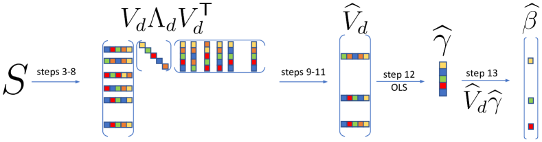
Figure 1: Graphical depiction of Algorithm 1. Solid colours represent nonzero matrix entries.

In this section, we introduce SuffPCR. The main idea of SuffPCR is to detect the relationship between the phenotype $Y$ and gene expression measurements $\mathbf{X}$ by making use of the (near) low-dimensional manifold that supports $\mathbf{X}$. In broad outline, SuffPCR first uses a tailored version of FPS to produce a row-sparse estimate $\widehat{\mathbf{V}}_{d}$, and then regresses $Y$ on the derived components to produce sparse coefficient estimates. SuffPCR for regression is stated in Algorithm 1 and summarized visually in Figure 1. For ease of exposition, we remind the reader that $Y$ and $\mathbf{X}$ are standardized so that $\mathbf{S}=\frac{1}{n}\mathbf{X}^{\mathsf{T}}\mathbf{X}$ is the correlation matrix.

The first issue is the time complexity of the original FPS algorithm. Essentially, FPS uses the same three steps depicted in lines 4, 5, and 6 in Algorithm 1.

1. $\mathbf{A}\leftarrow\mbox{Proj}_{\mathcal{F}^{d}}\left(\mathbf{B}-\mathbf{C}+\mathbf{S}/\lambda\right)$

2. $\mathbf{B}\leftarrow\mbox{Soft}(\mathbf{A}+\mathbf{C})$ where $\mbox{Soft}(b)=\mbox{sign}(b)\max\{|b|-1,\ 0\}$

3. $\mathbf{C}\leftarrow\mathbf{C}+\mathbf{A}-\mathbf{B}$.

The only difference here between our implementation and that in FPS is in step 4. Each of these steps takes a matrix and produces another matrix, where the matrices have $p^{2}$ elements. The second and third steps are computationally simple (element-wise soft-thresholding and matrix addition). But the first, $\mbox{Proj}_{\mathcal{F}^{d}}(\mathbf{Q})$, is more challenging. The solution requires computing the eigendecomposition of $\mathbf{Q}$, an $\mathcal{O}(p^{3})$ operation, and then modifying the eigenvalues of $\mathbf{Q}$ through the solution of a piecewise linear equation in $\tau$: $\mathbf{\Lambda}^{2}_{i,+}(\mathbf{Q})=\min\{\max\{\mathbf{\Lambda}^{2}_{i}(\mathbf{Q})-\tau,\ 0\},\ 1\},$ with $\tau$ such that $\sum_{i=1}^{\min\{n,p\}}\mathbf{\Lambda}^{2}_{i,+}(\mathbf{Q})=d$. The final result is then reconstructed as $\mathbf{A}=\mathbf{U}(\mathbf{Q})\mathbf{\Lambda}^{2}_{+}(\mathbf{Q})\mathbf{U}(\mathbf{Q})^{\mathsf{T}}$. Because of the cubic complexity in $p$, the authors suggest the number of features should not exceed one thousand. But typical transcriptomics data has many thousands of gene measurements, and preliminary selection of a subset is suboptimal, as illustrated above. Due to the form of the piecewise solution, most eigenvalues will be set to 0. Thus, while we will generally require more than $d$ eigenpairs, most are unnecessary, certainly fewer than $\min\{n,p\}$. Our implementation computes only a handful of eigenvectors corresponding to the largest eigenvalues, rather than all $p$. If we compute enough to ensure that some $\mathbf{\Lambda}^{2}_{i,+}(\mathbf{Q})$ will be 0, then the rest are as well. Our implementation uses Augmented Implicitly Restarted Lanczos Bidiagonalization [AIRLB, 2] as implemented in the irlba package [3], though alternative techniques such as those in Homrighausen and McDonald [23], Gittens and Mahoney [15] may work as well. We provide a more detailed discussion in the Supplement.

For moderate problems ($n,p\approx 100$), the truncated eigendecomposition with AIRLB rather than the full eigendecomposition leads to a three-fold speedup while the further incorporation of specialized initializations leads to an eight-fold improvement without any discernable loss of accuracy (results on a 2018 MacBook Pro with 2.7 GHz Quad-Core processor and 16GB of memory running maxOS 10.15). The results are similar when $p=5000$, though the same experiment on a high-performance Intel Xeon E5-2680 v3 CPU with 12 cores, 256GB of memory, and optimized BLAS were somewhat less dramatic (improvements of three-fold and four-fold respectively). For large RNA-Seq datasets ($p\approx 20000$), we observed a nearly ten-fold improvement in computation time.

The second issue is that the Fantope constraint in Equation (4) ensures only that $\mbox{tr}(\mathbf{V}\mathbf{V}^{\mathsf{T}})=d$ but not that the number of rows with non-zero $l_{2}$-norm is small. This feature of the convex relaxation results in many rows with small, but non-zero, row-norm resulting in dense estimates of $\beta^{*}$. Thus, to make the final estimator $\widehat{\mathbf{V}}_{d}$ sparse, we hard-threshold rows in $\widehat{\mathbf{V}}_{d}$ whose $\ell_{2}$ norm is small, as illustrated in line 9, 10, and 11 in Algorithm 1. From empirical experience, we have found that there is often a strong elbow-type behavior in the row-wise $\ell_{2}$ norm of $\widehat{\mathbf{V}}_{d}$, similar to the Skree plot used to choose $d$ in standard PCA. Therefore, we develop a simple procedure, Algorithm 2, to find the best threshold automatically. Essentially, it calculates the empirical derivative of the observation-weighted variances on each side of a potential threshold and maximizes their difference, resulting in signal and noise groups. We set the rows in $\widehat{\mathbf{V}}_{d}$ corresponding to the noise to 0. SuffPCR is also amenable for solving other generalized linear models. For example, replacing line 12 in Algorithm 1 with logistic regression solves classification problems.

1:  Input: a $p$-vector $l$

2:  for $i\in 1,\cdots,p$ do

3:     $T_{n}[i]=\texttt{var}(l[1:i])$

4:     $T_{s}[i]=\texttt{var}(l[(i+1):p])$

5:     $T[i]=i*T_{n}[i]+(p-i)T_{s}[i]$

6:     $\delta[i]=T[i]-T[i-1]$ $\rhd$ empirical derivative of $T$

7:  end for

8:  Set $i^{*}=\operatorname*{argmin}_{i}\{\delta[i]-\delta[i-1]>\texttt{mean}(|\delta[1:(i-1)]|)\}$

9:  Return: $t=l[i^{*}]$

Algorithm 2 Find a $t$ to hard-threshold $l$

3 Empirical evaluations

In this section, we show how SuffPCR performs on synthetic data and on real public genomics datasets relative to state-of-the-art methods. Section 3.1 first presents a generative model for synthetic data and motivates the assumptions required for our theoretical results in Section 4. We include here one synthetic experiment under conditions favorable to SuffPCR relative to SPC. We also investigate conditions favorable to SPC, the influence of tuning parameter selection, and the effect of the signal to noise ratio but defer these to the Supplement. Section 3.2 uses the NSCLC data as the $\mathbf{X}$ matrix, but creates the response from a linear model. Section 3.3 reports the performance of SuffPCR on 5 public genomics datasets. The supplement includes similar results for binary survival-status outcomes. Across most settings in both synthetic and real data, SuffPCR outperforms all competitors in prediction mean-squared error and is able to select the true genes (those with $\beta^{*}\neq 0$) more accurately. An R package implementing SuffPCR and raw data are freely available at https://github.com/dajmcdon/suffpcr. Package documentation may be viewed at https://dajmcdon.github.io/suffpcr.

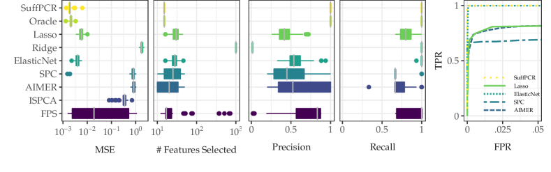
Figure 2: This figure compares the performance of SuffPCR against alternatives when the features come from a row-sparse factor model under favorable conditions for SuffPCR. Boxplots and receiver operating characteristic (ROC) curve (far right figure) are over 50 replications. We have omitted the other methods from the ROC curve for legibility, but their behavior is similar to lasso. TPR and FPR stand for True/False Positive Rate respectively. Note that (as one would expect from the simulation conditions), SPC has the worst performance in terms of the ROC curve while both SuffPCR and Elastic net have AUC of almost 1.

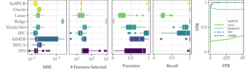
Figure 3: This figure compares the performance of SuffPCR against alternatives when the features come from a row-sparse factor model extracted from the NSCLC data. Boxplots and ROC curve (far right figure) are over 50 replications. In terms of the ROC curve, SPC and AIMER has the best performance, though SuffPCR is not far behind. But note that SPC has much worse precision and recall.

3.1 Synthetic data experiments

We generate data from the multivatiate Gaussian linear model $y_{i}=x_{i}^{\mathsf{T}}\beta^{*}+\epsilon_{i},$ where $x_{i}\sim\mbox{N}_{p}(0,\mathbf{\Sigma})$, $\beta^{*}$ is the $p$-dimensional regression coefficient, $\epsilon_{i}\sim\mbox{N}(0,\sigma_{y}^{2})$. We impose an orthogonal factor model for the covariates $x_{i}=u^{\mathsf{T}}_{i}\mathbf{\Lambda}_{d}\mathbf{V}_{d}^{\mathsf{T}}+e_{i},$ where $u_{i}$ are generated from $\mbox{N}_{d}(0,\mathbf{I}_{d})$ independently, $\mathbf{\Lambda}_{d}$ is a diagonal matrix with entries $(\lambda_{1},\ldots,\lambda_{d})$ in descending order, and $\mathbf{V}_{d}\in\mathbb{R}^{p\times d}$ with $\mathbf{V}_{d}^{\mathsf{T}}\mathbf{V}_{d}=\mathbf{I}_{d}$. The vector $e_{i}\in\mathbb{R}^{n}$ has i.i.d. $\mbox{N}(0,\sigma_{x}^{2})$ entries independent of $u_{i}$, and $\sigma_{x}>0$. We assume $\mathbf{V}_{d}$ is row sparse with only $s$ rows containing non-zero entries. These non-zero rows are the “true” features to be discovered, and they correspond to $\beta^{*}\neq 0$.

It is important to note that, under this model, the rows of $\mathbf{X}$ follow a multivariate Gaussian distribution independently, with mean 0 and full-rank covariance $\mathbf{\Sigma}=\mathbf{V}\mathbf{L}\mathbf{V}^{\mathsf{T}}$ whenever $\sigma^{2}_{x}>0$. Here the columns of $\mathbf{V}$ are orthonormal eigenvectors on $\mathbb{R}^{p}$ and the eigenvalues are $l_{1}\geq\cdots\geq l_{p}\geq 0$. Straightforward calculation shows that the first $d$ columns in $\mathbf{V}$ are the same as the right singular vectors $\mathbf{V}_{d}$ in the signal component of $\mathbf{X}$. Furthermore, $l_{i}=\lambda_{i}^{2}\mathbf{1}(i\leq d)+\sigma^{2}_{x}$, $i=1,\ldots,p$.

We generate $y\in\mathbb{R}^{n}$ as a linear function of the latent factors $\mathbf{U}_{d}$ with additive Gaussian noise: $y=\mathbf{U}_{d}\Theta+z,$ where $\Theta$ is the regression coefficient, and $z_{i}$ are i.i.d. $\mbox{N}(0,\sigma^{2}_{y})$, $i=1,\ldots,n$, independent of $\mathbf{X}$. Under this model the population marginal correlation between each feature in $\mathbf{X}$ and $y$ is $\Phi=\mathbf{V}_{d}\mathbf{\Lambda}_{d}\Theta,$ and the population ordinary least squares coefficient of regressing $y$ on $\mathbf{X}$ is $\beta^{*}=\mathbf{V}_{d}\mathbf{L}_{d}^{-1}\mathbf{\Lambda}_{d}\Theta.$ Note that the number of non-zero $\beta^{*}$ is $s$, because $\mathbf{V}_{d}$ has only $s$ rows with non-zero entries.

In all cases, we use $n=100$ observations and $p=1000$ features, generating three equal-sized sets for training, validation, and testing. We use prediction accuracy on the validation set to select tuning parameters for all methods. For the case of SuffPCR, this means only $\lambda$, because we choose $t$ with Algorithm 2 and set $d=3$. We use the test set for evaluating out-of-sample performance. Each simulation is repeated 50 times. Results with $n=200$ and $p=5000$ were similar. Algorithm 3 makes this entire procedure more explicit.

We compare SuffPCR with a number of alternative methods. The Oracle estimator uses ordinary least squares (OLS) on the true features and serves as a natural baseline: it uses information unavailable to the analyst (the true genes) but represents the best method were that information available. We also present results for Lasso [42], Ridge [22], Elastic Net [50], SPC [5], AIMER [11], ISPCA [39], and PCR using FPS directly without feature screening (using Algorithm 1 without step 9, 10 and 11). For ISPCA, we use the dimreduce R package to estimate the principal components before performing regression. For all competitors, we choose any tuning parameters that do not have default values using the validation set. Examples are $\lambda$ in Lasso, Ridge, and Elastic Net or the initial thresholding step in SPC. We use the correct embedding dimension ($d=3$) whenever this is meaningful. Additional experiments are given in the Supplement. There, we investigate conditions favourable to SPC, the choice of $d$, and the impact of different SNR choices.

1:  Input: $n=100$, $p=1000$, $r=5$, $d=3$, $\mathrm{SNR}_{x}=\mathrm{SNR}_{y}=5$.

2:  Generate i.i.d. $\textrm{N}(0,1)$ $\mathbf{U}\in\mathbb{R}^{n\times d}$, $\mathbf{E}\in\mathbb{R}^{n\times p}$, $z\in\mathbb{R}^{n}$.

3:  Set $\mathbf{\Lambda}_{d}=\textrm{diag}((d,\ d-1,\ldots,1))\in\mathbb{R}^{d\times d}$.

4:  Generate i.i.d. $\textrm{N}(0,1)$ $\widetilde{\mathbf{V}}\in\mathbb{R}^{d\times d}$ and orthogonalize the columns.

5:  Extend $\widetilde{\mathbf{V}}\in\mathbb{R}^{s\times d}$ by repeating each row $r$ times ($s=rd$).

6:  Set $\mathbf{V}^{\mathsf{T}}_{d}=[\widetilde{\mathbf{V}}^{\mathsf{T}}\;\mathbf{0}]\in\mathbb{R}^{d\times p}$.

7:  Generate i.i.d. $\textrm{N}(0,1)$ $\tilde{\Theta}\in\mathbb{R}^{d-1}$.

8:  Set $\Theta_{d}=-\left(\sum_{i=1}^{d-1}\widetilde{\mathbf{V}}^{\mathsf{T}}_{ri}\mathbf{\Lambda}_{ii}\tilde{\Theta}_{i}\right)/(\widetilde{\mathbf{V}}_{rd}\mathbf{\Lambda}_{dd})$.

9:  Set $\Theta=[\tilde{\Theta}^{\mathsf{T}}\;\Theta_{d}]^{\mathsf{T}}$.

10:  Set $\beta^{*}=\mathbf{V}_{d}\mathbf{L}_{d}^{-1}\mathbf{\Lambda}_{d}\Theta$.

11:  Set $\sigma^{2}_{x}=\textrm{tr}(\mathbf{\Lambda}_{d}^{2})/(p\mathrm{SNR}^{2}_{x})$

12:  Set $\sigma^{2}_{y}=\left(\beta^{*\mathsf{T}}\mathbf{V}_{d}^{\mathsf{T}}\mathbf{\Lambda}_{d}^{2}\mathbf{V}_{d}\beta^{*}+\sigma^{2}_{x}\lVert\beta^{*}\rVert_{2}^{2}\right)/(n\mathrm{SNR}^{2}_{y})$.

13:  Set $\mathbf{X}=\mathbf{U}_{d}\mathbf{\Lambda}_{d}\mathbf{V}_{d}^{\mathsf{T}}+\sigma_{x}\mathbf{E}$ and $y=\mathbf{U}_{d}\Theta+\sigma_{y}z$

Algorithm 3 Generate synthetic data

3.1.1 Conditions favorable to SuffPCR

The first setting is designed to show the advantages of SuffPCR relative to alternative methods, especially SPC. We note that other methods that employ screening by the marginal correlation [11, 39] will have similar deficiencies. Because SPC works well if Equation (1) holds, we design $\bm{\Sigma}$ to violate this condition and set the first 15 features to have non-zero $\beta^{*}$ but allow only the first 10 features to have non-zero correlation with the phenotype. This behaviour is achieved with line 8 of Algorithm 3. By solving this equation in one unknown component of $\Theta$, we force $\Phi=0$ for the third group of 5 components. Thus, as described in Section 2, Equation (1) will not hold: some $\Phi_{j}=0$ but $\beta^{*}_{j}\neq 0$. We set the true dimension of the subspace as $d=3$, and we use the correct dimension for methods based on principal components.

Figure 2 shows the performance of SuffPCR and state-of-the-art alternatives. In addition to reporting each method’s prediction MSE on the test set, we also show the number of features selected, precision, recall, and the ROC curve. The ISPCA implementation does not select features. In this example, SuffPCR actually outperforms the oracle estimator, attaining smaller MSE while generally selecting the correct features. This seemingly implausible result is likely because the variance of estimating OLS on 15 features is large relative to that of estimating the low-dimensional manifold followed by 3 regression coefficients. SuffPCR has a clear advantage over all the alternative methods, especially SPC which is 3 orders of magnitude worse. SPC works so poorly because it ignores 5 features. ISPCA has slightly lower MSE than SPC. Ridge is the worst, due to fitting a dense model when a sparse model generated the data. SuffPCR reduces MSE significantly relative to simply using FPS due to more accurate feature selection. The right plot in Figure 2 further shows the ROC curve for SuffPCR, Lasso, Elastic Net, SPC and AIMER in which we can easily vary the tuning parameter and select various numbers of features. SuffPCR and AIMER have a perfect ROC curve, while the other 3 methods are unable to identify 5 features. We undertake a similar exercise under conditions favorable to SPC in the Supplement.

3.2 Semi-synthetic analysis with real genomics data

The simulations in Section 3.1 explore various scenarios for the data generation process and show the performance of SuffPCR relative to the alternatives, however, they do not use any real genomic data. In this section, rather than fully generating $\mathbf{X}$, we create a semi-synthetic analysis wherein only the phenotypes are generated. We first performed PCA on the NSCLC data [27] and note that the first two empirical eigenvalues are relatively large, so we chose the number of PCs to be $d=2$. We keep the top 20 rows in the empirical $\mathbf{V}$ which have the largest norm and set the rest to 0. We then recombine and add noise. The phenotype is constructed as in the previous simulations, and the SNR is calibrated as in Section 3.1.1. Figure 3 shows the results analogous to those in Figure 2. SuffPCR continues to perform well relative to alternatives, though here, FPS has similar MSE, albeit poor feature selection.

3.3 Analysis of real genomics data

We analyze 5 microarray datasets that are publicly available and widely used as benchmarks. Four of the datasets present messenger RNA (mRNA) abundance measurements from patients with breast cancer [44, 34], diffuse large B-cell lymphoma (DLBCL) [40], and acute myeloid leukemia (AML) [6], and the fifth reports microRNA (miRNA) levels from non-small cell lung cancer (NSCLC) patients [27]. The features in $\mathbf{X}$ are gene expression measurements from microarrays. In the Supplement, we apply SuffPCR to predict COVID-19 viral load from RNA-Seq data.

The phenotypes $Y$ are censored survival time in all cases, though some of the datasets also contain binary survival status indicators. Because the real valued phenotype is non-negative and right censored, we follow common practice and transform $Y$ to $\log(Y+1)$. Each observation is a unique patient. The first breast cancer dataset has 78 observations and 4751 genes, the second has 253 observations and 11331 genes, DLBCL has 240 observations and 7399 genes, AML has 116 observations and 6283 genes, and NSCLC has 123 observations and 939 genes.

We randomly split each dataset into 3 folds for training, validation, and testing with proportions $40\%$, $30\%$ and $30\%$ respectively. We set the number of components $d=3$ and search over 5 log-linearly spaced $\lambda$ values. Other choices for $d$ and $\lambda$ yield similar results. We train all methods on the training set, use the validation set to choose any necessary tuning parameters, and report performance of each method on the test set. We repeat the entire process (data splitting, validation, and testing) 10 times to reduce any bias induced by the random splits. In all cases, all methods were tuned to optimize validation-set MSE.

Table 2 shows the average prediction MSE and the average number of selected features for SuffPCR and any alternative methods that perform feature selection. SuffPCR works better than all the alternative methods on 4 out of 5 datasets with a comparatively small number of features selected. The DLBCL data is difficult for both sparse and PC-based methods. As described in Section 2.3, FPS cannot be used for these data sets because of the number of genes. Non-sparse alternatives have much smaller MSE, suggesting that many genes may play a roll in mortality rather than only a subset. SPCA is designed to maximize the variance explained by the principal components subject to a penalty on the non-sparsity, and it does not seem to work well in regression tasks. DSPCA has relatively low prediction MSE, and it does in principle perform feature selection, though it generally produces a dense model. While Ridge, Random Forests and SVM predict well in general, they do not perform any feature selection, which is a key objective here, so show their MSE in the Supplement.

To assess the potential relevance of the genes selected by SuffPCR to the cancer type from which they were identified, we further explored the DLBCL data and extracted the selected genes. (We do the same with AML in the Supplement.) We first find the best $\lambda$ via 5-fold cross-validation on all the data and then train SuffPCR with this $\lambda$. Our model selects 87 features corresponding to 32 unique genes and 2 expressed sequence tags (ESTs) for DLBCL. Seventeen of the identified genes encode ribosomal proteins, overexpression of which is associated with poor prognosis [13]. A further 9 genes encoding major histocompatibility complex class II (MHCII) proteins were detected, a notable finding in light of the fact that MHCII downregulation is a means by which some DLBCLs evade the immune system [10]. Discovering these large groups of similarly functioning genes illustrates the benefits of SuffPCR relative to alternatives. CORO1A encodes the actin-binding tumor suppressor p57/coronin-1a, the promoter of which is often hypermethylated, and therefore likely silenced in DLBCL [29]. FEZ1 expression has been used in a prognostic model [31]. RAG1, encoding a protein involved in generating antibody diversity, can induce specific genetic aberrations found in DLBCL [33]. RYK encodes a catalytically dead receptor tyrosine kinase involved in Wnt signaling and CXCL5 encodes a chemokine. To our knowledge, neither gene has been implicated in DLBCL and thus may be of interest for further exploration. EST Hs.22635 (GenBank accession AA262469) corresponds to a portion of ZBTB44, which encodes an uncharacterized transcriptional repressor, while EST Hs.343870 (GenBank accession AA804270) does not appear to be contained within an annotated gene. The Supplement lists the selected genes and associated references. A separate listing of the genes encoding ribosomal and MHCII proteins are given in the Supplement.

	Breast Cancer1			Breast Cancer2			DLBCL			AML			NSCLC
Method	MSE	feature#		MSE	feature#		MSE	feature#		MSE	feature#		MSE	feature#
SuffPCR	0.5980	80		0.4168	121		0.7073	48		1.9568	75		0.1970	27
Lasso	0.7141	7		0.4622	39		0.6992	31		2.0998	3		0.2263	4
ElasticNet	0.6845	41		0.4517	104		0.6869	87		2.0820	5		0.2332	20
SPC	0.6188	59		0.4179	823		0.7677	67		2.3237	62		0.2795	62
ISPCA	0.8647	NA		0.5882	NA		0.9441	NA		2.3109	NA		0.2408	NA
AIMER	0.6629	76		0.4192	795		0.7003	76		1.9737	36		0.2120	50
SPCA	17.0965	212		4.7239	38		2.5980	652		31.11	1043		0.9757	387
DSPCA	0.6132	4374		0.4557	7880		0.7249	1342		1.9781	2742		0.2041	305

Table 2: Prediction MSE and number of selected features for regression of survival time on gene expression measurements

4 Theoretical guarantees

When the sparse factor model described in Section 3 is true, SuffPCR enjoys near-optimal convergence rates. We now make the necessary assumptions concrete and note that some can be weakened.

• $Y_{i}=X_{i}^{\mathsf{T}}\beta^{*}+\epsilon_{i}$, $i=1,\ldots,n$, where $\epsilon_{i}\sim\mbox{N}(0,\sigma_{y})$, $\sigma_{y}>0$.

• $X_{i}\sim\mbox{N}_{p}(0,\bm{\Sigma})$, $i=1,\ldots,n$.

• $\bm{\Sigma}=\mathbf{VLV}^{\mathsf{T}}$, is symmetric, $\mathbf{V}^{\mathsf{T}}\mathbf{V}=\mathbf{I}_{p}$, $\mathbf{L}$ is diagonal.

• $l_{i}=\lambda_{i}^{2}\mathbf{1}(i\leq d)+\sigma_{x}^{2}$ and $\lambda_{1}-\lambda_{d}:=\phi>0$.

• $\lVert\mbox{diag}\left(\mathbf{V}_{d}\mathbf{V}_{d}^{\mathsf{T}}\right)\rVert_{0}\leq s$ and $\min_{j}\left\{(\mathbf{V}_{d}\mathbf{V}_{d}^{\mathsf{T}})_{jj}\vee 0\right\}>2\tau$.

• as $n,p\rightarrow\infty$, $n>(s^{2}+d)\log(p)$ eventually.

Assumptions A1–A4 are the same as those used in Section 3.1 to generate data from a linear factor model. Assumption A5 says that the number of true nonzero coefficients $\beta^{*}$ must be no more than $s$ and that the size of the associated components must be large enough. Assumption A6 means that eventually, we must have at least as many observations $n$ as a logarithmic function of $p$ times the true number of components plus the square of the number of nonzero $\beta^{*}$ coefficients.

Theorem 1.

Suppose assumptions A1 to A6 hold and let $\widehat{\beta}$ be the estimate produced by SuffPCR with $\lambda=c\lambda_{1}\sqrt{\log(p)/n}$ and $t<2\tau$ where $t$ is the threshold used in Algorithm 1 and $\tau$ is given in A5. Then

$$\frac{1}{n}\lVert\mathbf{X}(\widehat{\beta}-\beta^{*})\rVert^{2}_{2}=\mathcal{O}_{P}\left(\frac{(s^{2}+d)\log(p)}{n}\right).$$

Theorem 2.

Suppose assumptions A1 to A6 hold and let $\widehat{\beta}$ be the estimate produced by SuffPCR with $\lambda=c\lambda_{1}\sqrt{\log(p)/n}$ and $2\tau>t>\tau$ where $t$ is the threshold used in Algorithm 1 and $\tau$ is given in A5. Then

$$\left|\mathrm{supp}\left(\widehat{\beta}\right)\bigtriangleup\mathrm{supp}\left(\beta^{*}\right)\right|=\mathcal{O}_{P}\left(\frac{s^{2}\log(p)}{n}\right),$$

where $A\bigtriangleup B=A/B\cup B/A$ is the symmetric difference operator and $\mathrm{supp}$ denotes the support set.

In both results above, $c$ is a positive number (possibly different between the two) that is independent of $n$ and $p$, but may depend on any of the other values given in A1–A6. Theorem 1 gives a convergence rate for the prediction error of SuffPCR comparable to that of Lasso though with explicit additional dependence on $d$. Under standard assumptions with fixed design, this dependence would not exist for Lasso. On the other hand, our results are for random design with $d$ small, along with different constants absorbed by the big-$\mathcal{O}$. Theorem 2 shows that our procedure can correctly recover the set of nonzero $\beta^{*}$ as long as the threshold $t$ is chosen correctly. We note that this result is a direct consequence of Vu et al. [46, Theorem 3.2]. In practice, the condition $2\tau>t>\tau$ cannot be verified, although the “elbow” condition we employ in the empirical examples seems to work well. Finally, we emphasize that, as is standard in the literature, these results are for asymptotically optimal tuning parameters $\lambda,\ t$ rather than empirically chosen values. The proof of Theorem 1 is given in the Supplement. These results suggest that SuffPCR is nearly optimal as $p$ and $n$ grow.

5 Discussion

High-dimensional prediction methods, including regression and classification, are widely used to gain biological insights from large datasets. Three main goals in this setting are accurate prediction, feature selection, and computational tractability. We propose a new method called SuffPCR which is capable of achieving these goals simultaneously. SuffPCR is a linear predictor on estimated sparse principal components. Because of the sparsity of the projected subspace, SuffPCR usually selects a small number of features. We conduct a series of synthetic, semi-synthetic and real data analyses to demonstrate the performance of SuffPCR and compare it with existing techniques. We also prove near-optimal convergence rates of SuffPCR under sparse assumptions. SuffPCR works better than alternative methods when the true model only involves a subset of features.

Funding

The authors gratefully acknowledge support National Science Foundation (grant DMS–1753171 to DJM) the National Institutes of Health (grant R35GM128631 to GEZ) and the National Sciences and Engineering Research Council of Canada (NSERC) (grant RGPIN-2021-02618 to DJM).

Appendix A Genetics data discussion

In this section we provide more details on the 5 standard genetics data sets discussed in the manuscript. We then apply our methodology to one/two additional data sets which are less well studied in the literature.

A.1 Detailed description

In the manuscript (and below in Section C.4), we analyze 5 microarray datasets that are publicly available and widely used as benchmarks. Four of the datasets present messenger RNA (mRNA) abundance measurements from patients with breast cancer [44, 34], diffuse large B-cell lymphoma (DLBCL) [40], and acute myeloid leukemia (AML) [6], and the fifth reports microRNA (miRNA) levels from non-small cell lung cancer (NSCLC) patients [27].

These data sets have between about 80 and 250 patients with expression measurements on 900 to 11000 genes. Table 3 gives specific statistics about each dataset.

Name	$n$ (patients)	$p$ (genes)
Breast cancer [44]	78	4751
Breast cancer [34]	253	11331
DLBCL [40]	240	7399
AML [6]	116	6283
NSCLC [27]	123	939

Table 3: Summary of canonical datasets

The AML data was originally collected and analyzed by [6]. They used complementary-DNA microarrays to measure gene expression from either peripheral-blood or bone marrow samples from 116 adults with AML. The gene expression measurements for the 6283 genes that were highly variable across patients are included. The observed outcomes are the (possibly right-censored) survival time in days as well as a binary indicator for whether or not the patient died.

The first set of breast cancer data from [44] is based on 78 sporadic lymph-node-negative patients. The authors derived cRNA from snap-frozen tumor samples and pooled across each of the sporadic carcinomas. The 4751 available genes were significantly regulated across the patients (showing at least a two-fold difference across at least 5 patients). The outcome is the follow-up time (in months) for metastases as well as a binary indicator for whether prognosis was “good” (no metastases within 5 years) or “poor”.

The second set of breast cancer gene expression measurements is based on 253 patients who’s cancer tissues were sequenced for the p53 mutation [34]. A binary variable for the presence of the p53 mutation is missing for two patients, which were removed from further analysis. The regression exercise focuses on the right-censored survival time (measured in years). The measured gene expressions come from Affymetrix high-density oligonucleotide arrays. A number of other clinical variables are also present in the data contained in the R package (https://github.com/dajmcdon/suffpcr).

The DLBCL data was collected by [6] and contains Biopsy samples from 240 patients with gene expression measurements from DNA microarrays. The microarrays were constructed from 12,196 clones of cDNA then used to quantify the expression of mRNA in the tumors. Genes with significant differential expression across patients were included. The response is survival time after chemotherapy in years as well as binary survival status (57% of patients died).

Finally, the NSCLC dataset was analysed by [27]. The expression measurements consist of from paired (tumor and non-tumor) micro RNA collected from 123 cancer patients. The response variable is the time to relapse in years. Other clinical variables are also available.

Appendix B Application to COVID-19 Data

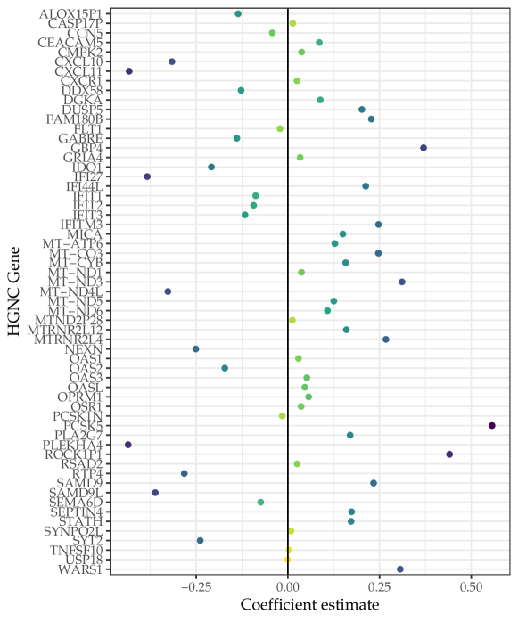
Figure 4: Coefficient estimates from SuffPCR on RNA-Seq measurements of COVID-19-positive patients. The colour corresponds to the magnitude.

In this section, we apply our methods to RNA-Seq data for COVID-19-positive patients. As a developing disease, biological analysis remains highly desirable, and so to facilitate this sort of undertaking, recent work has endeavoured to collect and distribute this data publicly [48].

Here, we examine the data collected by Lieberman et al. [30], and examine how well RNA-Seq measurements predict viral load. The data contains results for 430 PCR-confirmed COVID-positive patients and 54 negative controls. Lieberman et al. [30] examines both differential expression between positives and controls and the viral load of the positive patients, while we focus on only the viral load. Of the 430 confirmed positives, 413 have reported usable measurements. Viral load in this case is measured through a proxy: the cycle threshold (Ct) of the SARS-CoV-2 nucleocapsid gene region 1 (N1) target from a PCR test. Larger Ct values indicate more cycles are required to detect the N1 target, and thus, likely indicate lower viral load. While Lieberman et al. [30] bin this continuous measurement into “high” and “low” groups to undertake differential analysis, our methodology directly models the continuous response. This allows for (1) increased ability to detect potentially predictive genes and (2) direct quantification of the effect of increased expression on viral load.

The raw expression measurements are preprocessed before being used in SuffPCR. First, we remove any genes whose median expression level across the 413 patients with Ct measurements is 0. This reduces the data from $\sim$36,000 genes to 9435. We then transform the raw counts using $\tilde{z}\mapsto\log(\tilde{z}+1)$. Finally, we centre and scale by the mean and standard deviation of the similarly transformed measurements from the healthy controls. Mathematically, if $\tilde{z}_{gt}$ is the vector of expression measurements for gene $g$ in the treatment group and $\tilde{z}_{gc}$ is the vector of expression measurements for the same gene in the control group, we form

$$x_{gt}=\frac{\log(\tilde{z}_{gt}+1)-\overline{z}_{gc}}{\textrm{sd}(z_{gc})},$$

where $\overline{z}_{gc}=\textrm{mean}(\log(\tilde{z}_{gc}+1))$ and $\textrm{sd}(z_{gc})=\textrm{sd}(\log(\tilde{z}_{gc}+1))$.

We apply SuffPCR to the $\mathbf{X}$ matrix formed by the columnwise concatenation of $x_{gt}$ with the N1 Ct as the response vector. We examined embedding sizes of $d\in\{3,\ 5,\ 15\}$ and $\lambda$ on a $\log_{10}$-spaced grid between 0 and 1. We chose both parameters using the minimum of the 5-fold cross-validation error. The result is shown in Figure 4 (here $d=15$). Our method selected 59 genes. Many of these with the largest magnitude (darkest colour) are similar to those described in [30]: the CXCL10 and 11 genes along with IDO1 and IFI27 are proinflammatory and/or interferon induced and may be related to the “cytokine storm” found in some patients [32]. Novel and potentially interesting PLEKHA4, which is strongly related to higher viral load, but more closely related to melanomas. PCS5K is more strongly expressed in patients with lower viral load. This gene encodes a proprotein convertase that may potentially help to clear the virus. ROCK1P1, also more strongly expressed in lower viral load patients, is not well understood.

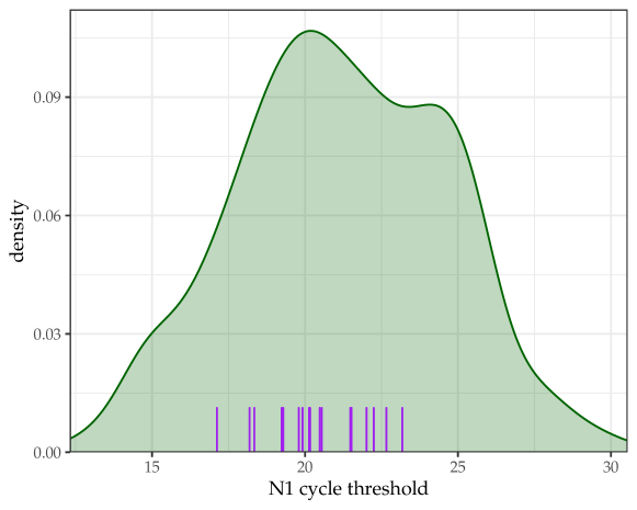
Figure 5: Density of observed N1 Ct values for 413 patients (green area) and predicted values for 27 positive patients with “Unknown” values (purple lines) based on SuffPCR estimated from the complete cases.

As mentioned above, 27 patients were positive but did not have a measured N1 Ct from the PCR test. These were also missing age and gender information. Using the fitted SuffPCR model, we can predict their missing N1 cycle thresholds. These predictions are shown in Figure 5. The green area shows a density estimate for the 413 patients with observed measurements while the purple lines display predicted values for those positive patients whose N1 Ct values are labeled “Unknown”. Because the data is missing, the accuracy of these predictions cannot be determined.

Appendix C Additional experiments and results for regression

C.1 Conditions favorable to SPC

This example is designed to show the performance of SuffPCR under favorable conditions for SPC. Here, the only alteration to the data generation process is that we set the first 10 features to have non-zero $\beta^{*}$, the same features which have non-zero marginal correlations with the phenotype. This is achieved using Algorithm 3 in the manuscript with a few alterations: (1) in line 5, we generate $\widetilde{\mathbf{V}}_{d}\in\mathbb{R}^{(d-1)\times 3}$ (recall that we have chosen $d=3$); and (2) we replace lines 7–9 by directly simulating $\Theta\in\mathbb{R}^{d}$ with i.i.d. standard normal entries.

Figure 6 gives the analogous results for this example. Here, SuffPCR has comparable MSE to SPC, which is the best, slightly better than the oracle as was the case for SuffPCR above. However, SPC is less likely to select the correct features, while SuffPCR selects the correct features most of the time. Furthermore, SuffPCR tends to select fewer features, and it has the best precision and recall (Ridge will always have recall equal to 1).

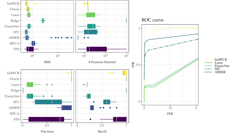
Figure 6: This figure demonstrates the performance of SuffPCR under favorable conditions for SPC. We have omitted the other methods from the ROC curve for legibility, but their behavior is similar to lasso.

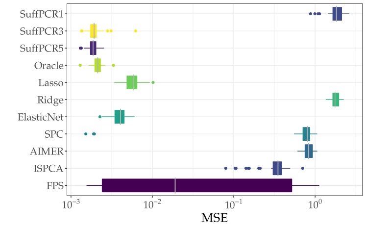
Figure 7: This figure compares the prediction MSE of SuffPCR with alternatives with different $d$ in SuffPCR.

C.2 Selecting tuning parameters

In SuffPCR, the tuning parameters are the penalty term $\lambda$, the dimension of the projected subspace $d$, and the threshold $t$. In all the simulations, we examine the same values of $\lambda$. When analyzing real datasets, our algorithm offers automatic calculation of potential values of $\lambda$ given the sample covariance matrix. In practice, the more penalty parameters we explore, the better the results could be assuming the sample size is large enough that risk estimation is not too volatile.

To demonstrate the importance of selecting $d$, we simulate the data with $d=3$ and set all the other parameters the same as in the first simulation. We estimate SuffPCR using $d\in\{1,\ 3,\ 5\}$ and display the results in Figure 7. When $d$ is smaller than the true value, it is hard for SuffPCR to capture all the information contained in $\mathbf{X}$, thus SuffPCR has terrible prediction MSE, worse than any other methods. When $d$ is larger than the true value, SuffPCR remains reasonable because its bias is small, but the variance will eventually increase as $d$ increases, diminishing performance. Selecting $t$ is not difficult in our simulations, so the results have been omitted, but it is less trivial in the real data settings.

C.3 Investigation of signal-to-noise ratio with synthetic data

In all or our synthetic examples, the data generating model has two sources of noise, one from constructing $\mathbf{X}$ corresponding to $\sigma_{x}$, and the other from constructing $Y$, denoted $\sigma_{y}$. This simulation aims to control the two noise sources separately to examine their effect on the performance of SuffPCR. Note that $\mathbf{X}$ is random unlike in standard prediction studies, so both sources of noise are important. We use $\textrm{SNR}_{x}$ and $\textrm{SNR}_{y}$ to denote the signal-to-noise ratio for $\mathbf{X}$ and $Y$ respectively. These are given by

$$\textrm{SNR}_{x} =\frac{\mathbb{E}\left[\left\lVert\mathbf{U}_{d}\mathbf{\Lambda}_{d}\mathbf{V}_{d}^{\mathsf{T}}\right\rVert_{F}\right]}{\mathbb{E}\left[\left\lVert\sigma_{x}\mathbf{E}\right\rVert_{F}\right]}=\sqrt{\frac{\mbox{tr}(\Lambda_{d}^{2})}{p\sigma_{x}^{2}}},$$ (5)

$$\textrm{SNR}_{y} =\frac{\mathbb{E}\left[\left\lVert\mathbf{X}\beta^{*}\right\rVert_{2}\right]}{\mathbb{E}\left[\left\lVert\sigma_{y}Z\right\rVert_{2}\right]}=\sqrt{\frac{\beta^{*\mathsf{T}}\mathbf{V}_{d}\mathbf{\Lambda_{d}^{2}}\mathbf{V_{d}^{\mathsf{T}}}\beta^{*}+\sigma_{x}^{2}\lVert\beta^{*}\rVert_{2}^{2}}{n\sigma_{y}^{2}}}.$$ (6)

Note that $\textrm{SNR}_{y}$ depends not only on $\beta^{*}$ but also on $\sigma_{x}$ and the linear manifold through $\mathbf{V}_{d}$.

We alter the values of $\textrm{SNR}_{x}$ and $\textrm{SNR}_{y}$ to generate $\mathbf{X}$ and $Y$ while everything else is as in the first simulation. Figure 8 shows the prediction MSE for all methods on four sets of simulated data for both high and moderate combinations of $\textrm{SNR}_{x}$ and $\textrm{SNR}_{y}$. When the SNR decreases, the prediction MSE of all the methods increases as expected. In all configurations, SuffPCR performs similarly to the oracle, better than Lasso or Elastic Net, while SPC is more similar to Ridge regression (though better). Interestingly, changing $\textrm{SNR}_{x}$ and $\textrm{SNR}_{y}$ has a similar impact on nearly all the methods except Ridge, SPC, AIMER, and ISPCA, which are nearly unaffected and uniformly worse by an order of magnitude.

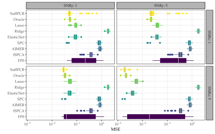
Figure 8: This figure compares the prediction MSE of SuffPCR with alternatives across different values of $\textrm{SNR}_{x}$ and $\textrm{SNR}_{y}$. The $x$-axis is on the log scale. Boxplots are over 50 replications.

C.4 Predictive genes/miRNA for additional cancers

Table 4 enumerates genes selected by SuffPCR on the DLBCL data, Table 5 lists the selected genes for AML, Table 6 lists the miRNA sequences selected by SuffPCR on the NSCLC data, while Table 7 lists all the features selected by SuffPCR on the Breast Cancer1 data. Table 8 gives the prediction MSE for Ridge, Random Forests and SVM for the 5 regression datasets we examine in Section 3.3 of the manuscript. These methods predict well in general, but they do not select features.

For AML we describe the related work summarized in Table 5 in more detail. Of the 4 discovered genes, 3 have been discussed in the literature. BPGM, encoding a multifunctional metabolic enzyme restricted to erythrocytes and placental cells, is upregulated in mouse models of AML [37]. PI4KB, encoding a lipid kinase, is amplified in breast cancer [47] and has been proposed to be a druggable AML-specific dependency [49]. LOC90379 encodes an uncharacterized protein that is highly immunogenic in ovarian cancer serum [16]. The fourth feature discovered, Hs.321434, is an EST (GenBank accession H96229) that corresponds to an intronic sequence of an uncharacterized long noncoding RNA (lncRNA), LOC101929579, and is thus of uncertain significance. Similar listings for the discovered genes for the NSCLC and Breast Cancer 1 data are given in the Supplement without the accompanying literature review.

Finally, Table 10 expands on the listing in the main document, listing the genes encoding ribosomal proteins and MHCII protein which predict DLBCL survival as selected by SuffPCR.

Gene	Related ?	Reference
Ribosomal protein genes (17)	✔	Ednersson et al. [13]
MHCII (9)	✔	de Charette and Houot [10]
CORO1A	✔	Li et al. [29]
FEZ1	✔	Liu et al. [31]
RAG1	✔	[33]
RYK	✗
CXCL5	✗
ESTs Hs.22635, Hs.343870	✗

Table 4: Predictive genes for DLBCL selected by SuffPCR.

Gene	Related ?	Reference
BPGM	✔	[37]
PI4KB	✔	[49]
EST Hs.321434	✗
LOC90379	✔	[16]

Table 5: Predictive genes for AML selected by SuffPCR.

#	Sequence	#	Sequence
1	hsa-miR-376c	21	hsa-miR-409-5p
2	hsa-miR-320c	22	hcmv-miR-US4
3	hsa-miR-299-3p	23	hsa-miR-376a
4	hsa-miR-154	24	hsa-miR-1471
5	hsa-miR-410	25	hsa-miR-411
6	hsa-miR-1182	26	bkv-miR-B1-5p
7	hsa-miR-136	27	hsa-miR-377
8	hsa-miR-379	28	hsa-miR-601
9	hsa-miR-765	29	hsa-miR-299-5p
10	hsa-miR-610	30	hsa-miR-543
11	hsa-miR-487a	31	hsa-miR-381
12	hsa-miR-136*	32	hsa-miR-329
13	hsv1-miR-H1	33	hsa-miR-760
14	hsa-miR-622	34	hsa-miR-409-3p
15	hsa-miR-659	35	hsa-miR-617
16	hsa-miR-376b	36	hsa-miR-758
17	hsa-miR-154*	37	hsa-miR-1183
18	hsa-miR-483-5p	38	hsa-miR-671-5p
19	hsa-miR-337-5p	39	hsa-miR-127-3p
20	hsa-miR-376a*

Table 6: RNA sequences selected by SuffPCR for NSCLC data.

#	Feature	#	Feature
1	NM_003118	15	NM_003247
2	Contig46244_RC	16	NM_004079
3	Contig55801_RC	17	NM_002775
4	M37033	18	NM_004369
5	NM_004385	19	NM_002985
6	Contig43613_RC	20	Contig43833_RC
7	Contig42919_RC	21	NM_005565
8	NM_016081	22	Contig52398_RC
9	NM_016187	23	NM_006889
10	Contig30260_RC	24	Contig66347
11	NM_000089	25	NM_000090
12	NM_000138	26	Contig25362_RC
13	NM_000393	27	NM_000560
14	Contig58512_RC	28	NM_001387

Table 7: Features selected by SuffPCR for Breast Cancer1 data.

	Breast Cancer1			Breast Cancer2			DLBCL			AML			NSCLC
Method	MSE	feature#		MSE	feature#		MSE	feature#		MSE	feature#		MSE	feature#
Ridge	0.6331	4751		0.4330	11331		0.6766	7399		2.0451	6283		0.2105	939
Random Forest	0.5519	4751		0.3976	11331		0.6613	7399		2.0276	6283		0.2059	939
SVM linear	0.6375	4751		0.4009	11331		0.7414	7399		2.5637	6283		0.2819	939
SVM RBF	0.5602	4751		0.4448	11331		0.6684	7399		2.0106	6283		0.2080	939

Table 8: Prediction MSE for alternative methods in real genomics data analysis.

Appendix D Extension to classification

SuffPCR is easily extended to solve classification tasks using logistic regression (or even other classification methods). We use logistic regression as an example to show how SuffPCR performs for classification tasks. Note that the algorithm is similar to Algorithm 1 except that step 12 is replaced by the objective of logistic regression.

D.1 Synthetic data for binary classification

We first use a simulation to demonstrate the generalization of SuffPCR to solve a binary classification problem. Using the same data generating model and parameters as in the favorable scenario in Section 3.1.1 of the manuscript, we generate $Y$ using the logistic function. As before, we choose tuning parameters with the validation set, and report the overall prediction accuracy on the test set.

Figure 9 shows the classification accuracy compared to the oracle (logistic regression on the true predictors), logistic lasso, logistic ridge, and logistic FPS (logistic regression on the estimated principal components from FPS). SuffPCR has very high classification accuracy on the test set relative to the alternative methods. We also simulate classification data analogously to the other scenarios discussed in the manuscript, and the results are very similar.

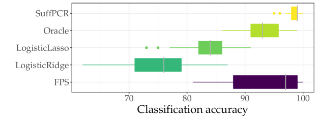
Figure 9: This figure compares the classification accuracy of SuffPCR with alternative methods. The $x$-axis shows the percentage of correct classifications on the test set. Boxplots are over 50 repeated simulations.

D.2 Analysis of real genomics data

We analyze 3 of the 5 real genomics datasets from Section 3.3 of the manuscript, which include a binary survival status. We use the same training test split process as in the manuscript and compare SuffPCR with logistic lasso and logistic ridge.

	Breast cancer1			DLBCL			AML
Method	Acc.%	feature #		Acc.%	feature #		Acc.%	feature #
SuffPCR	60.95	100		60.43	103		59.39	95
Logistic Lasso	60.00	7		56.86	5		57.57	9
Logistic Ridge	58.09	4751		61.00	7399		56.97	6283

Table 9: Accuracy of survival status prediction and number of selected genes for the classification tasks on real data. Results are averaged over 10 repeated iterations.

Table 9 shows the average classification accuracy and average number of selected genes in the classification tasks. The results in the classification tasks are similar to those in regression. Again, the DLBCL dataset tends to be difficult for both sparse and PC-based methods.

GenBank AN	description
M17886	ribosomal protein, large, P1
S79522	ribosomal protein S27a
X03342	ribosomal protein L32
D23661	ribosomal protein L37
M84711	ribosomal protein S3A
L06498	ribosomal protein S20
U14973	ribosomal protein S29
M17887	ribosomal protein, large P2
L04483	ribosomal protein S21
M64716	ribosomal protein S25
L19527	ribosomal protein L27
X66699	ribosomal protein L37a
U14970	ribosomal protein S5
X64707	ribosomal protein L13
U14971	ribosomal protein S9
M60854	ribosomal protein S16
NM_022551	ribosomal protein S18
X00452	major histocompatibility complex, class II, DQ alpha 1
X00457	major histocompatibility complex, class II, DP alpha 1
X62744	major histocompatibility complex, class II, DM alpha
U15085	major histocompatibility complex, class II, DM beta
M16276	major histocompatibility complex, class II, DQ beta 1
K01171	major histocompatibility complex, class II, DR alpha
M20430	major histocompatibility complex, class II, DR beta 5
M83664	major histocompatibility complex, class II, DP beta 1
K01144	CD74 antigen (invariant polypeptide of major
	histocompatibility complex, class II antigen-associated)

Table 10: A listing of the genes encoding ribosomal proteins and MHCII protein which predict DLBCL survival as selected by SuffPCR.

Appendix E Approximate singular value decomposition in Algorithm 1

To approximate the top $j$ eigenvalues of a symmetric matrix $\mathbf{A}$, we require the $k$-step (partial) Lanczos bidiagonalization $(j<k)$. For initial vector $p_{1}$, this is given by

$$\mathbf{AP}^{(k)} =\mathbf{Z}^{(k)}\mathbf{W}^{(k)},\;\mathbf{A}^{\mathsf{T}}\mathbf{Z}^{(k)}=\mathbf{P}^{(k)}\mathbf{W}^{(k),\mathsf{T}}+r^{(k)}e_{k}^{\mathsf{T}}$$ (7)

where $\mathbf{P}^{(k),\mathsf{T}}\mathbf{P}^{(k)}=\mathbf{Z}^{(k),\mathsf{T}}\mathbf{Z}^{(k)}=\mathbf{I}\in\mathbb{R}^{k\times k}$, $\mathbf{P}^{(k),\mathsf{T}}r^{(k)}=0$, $\mathbf{P}^{(k)}e_{1}=p_{1}$, and $\mathbf{W}^{(k)}$ is bidiagonal. Approximate eigenvectors and eigenvalues for $\mathbf{A}$ can then be computed using the SVD for $\mathbf{W}$, which is easy because of the bidiagonal structure. However, the accuracy is closely tied to the choice of the initial vector $p_{1}$ and can be measured by the norm of the residual vector $r^{(k)}$. AIRLB [2] essentially augments the SVD of $\mathbf{W}$ with additional information to reexpress $\mathbf{P}^{(k)}$, $\mathbf{Z}^{(k)}$ and $\mathbf{W}^{(k)}$. This process is repeated until the residual is deemed small enough.

If $p_{1}$ is in the span of the top $j$ eigenvectors of $\mathbf{A}$, then no iteration will be necessary, and the approximation is exact. So, within our ADMM, when the span of the eigenvectors for $\mathbf{B}-\mathbf{C}+\mathbf{S}/\rho$ is similar across iterations, previous iterates can be used as initializations for the restarted Lanczos procedure. Thus, as we loop through the ADMM steps, these initializations improve the speed subsequent decompositions.

This modification significantly improves the per-iteration efficiency of the algorithm while still converging in a few dozen iterations. Note that ADMM will still converge (though in perhaps more iterations) if some or all of the steps are implemented approximately [12]. In particular, by approximating the projection of $\mathbf{Q}$, $\mbox{Proj}_{\mathcal{F}^{d}}(\mathbf{Q})$, with $\widetilde{\mbox{Proj}}_{\mathcal{F}^{d}}(\mathbf{Q})$, ADMM will converge provided

$$\sum_{k=1}^{\infty}\left\lVert\mbox{Proj}_{\mathcal{F}^{d}}(\mathbf{Q}^{(k)})-\widetilde{\mbox{Proj}}_{\mathcal{F}^{d}}(\mathbf{Q}^{(k)})\right\rVert<\infty.$$

Nishihara et al. [36] suggests linear convergence for ADMM, and our experience is that this case remains linear despite the approximation.

Appendix F Proofs

To prove Theorem 1, we first need the following technical lemma.

Lemma 1.

Let $\bm{\Xi}=\mathbf{ZZ}^{\mathsf{T}}$ be the orthogonal projector on to the $d$-dimensional subspace of $\mathbb{R}^{p}$ spanned by $\mathbf{Z}$ with $\mathbf{Z}^{\mathsf{T}}\mathbf{Z}=\mathbf{I}_{d}$. Let $b\in\mathbb{R}^{n}$ and $\mathbf{A}\in\mathbb{R}^{n\times p}$. Then, defining $\widehat{x}:=\operatorname*{argmin}_{x}\left\lVert\mathbf{AZ}x-b\right\rVert_{2}^{2}$,

$$\mathbf{Z}\widehat{x} =\mathbf{Z}(\mathbf{AZ})^{+}b=(\mathbf{A}\bm{\Xi})^{+}b$$ (9)

$$=\operatorname*{argmin}_{y}\left\lVert\mathbf{A}\bm{\Xi}y-b\right\rVert_{2}^{2}=:\widehat{y},$$ (10)

where $\mathbf{Q}^{+}$ is the Moore-Penrose generalized inverse of $\mathbf{Q}$.

Proof of Lemma 1.

We have

$$\widehat{y} :=(\mathbf{A}\bm{\Xi})^{+}b=\bm{\Xi}(\mathbf{A}\bm{\Xi})^{+}b=\mathbf{ZZ}^{\mathsf{T}}(\mathbf{AZZ}^{\mathsf{T}})^{+}b$$ (11)

$$=\mathbf{ZZ}^{\mathsf{T}}\mathbf{Z}(\mathbf{AZ})^{+}b=\mathbf{Z}(\mathbf{AZ})^{+}b=:\mathbf{Z}\widehat{x}.$$ (12)

Here, the first equality is a standard property of idempotent matrices and the third follows from [18, Thm. 20.5.6]. ∎

Proof of Theorem 1.

Write $\bm{\Pi}=\mathbf{V}_{d}\mathbf{V}_{d}^{\mathsf{T}}$ and $\widehat{\bm{\Pi}}=\widehat{\mathbf{V}}_{d}\widehat{\mathbf{V}}_{d}^{\mathsf{T}}$ for the orthogonal projectors onto the column span of the population quantity $\mathbf{V}_{d}$ and the estimate produced by Algorithm 2 respectively. Let

$$\tilde{\gamma}=\operatorname*{argmin}_{\gamma}\left\lVert\mathbf{XV}_{d}\gamma-Y\right\rVert_{2}^{2},$$

and define $\tilde{\beta}=\mathbf{V}_{d}\tilde{\gamma}$. Note that $\beta_{*}\in\mbox{col}(\mathbf{V}_{d})$ and $\widehat{\beta}\in\mbox{col}(\widehat{\mathbf{V}}_{d})$ as $\beta_{*}=\mathbf{V}_{d}\mathbf{L}_{d}^{-1}\bm{\Lambda}_{d}\Theta=:\mathbf{V_{d}}r$ and $\widehat{\beta}=\mathbf{\widehat{V}}_{d}\widehat{\gamma}$. Then,

$$\left\lVert\mathbf{X}(\beta_{*}-\widehat{\beta})\right\rVert_{2}^{2}$$ (13)

$$=\left\lVert\mathbf{X}(\beta_{*}-\tilde{\beta})\right\rVert_{2}^{2}+\left\lVert\mathbf{X}(\tilde{\beta}-\widehat{\beta})\right\rVert_{2}^{2}$$ (14)

$$=\left\lVert\mathbf{X}\left(\mathbf{V}_{d}\gamma_{*}-\mathbf{V}_{d}\tilde{\gamma}\right)\right\rVert_{2}^{2}+\left\lVert\mathbf{X}\left(\mathbf{V}_{d}\tilde{\gamma}-\widehat{\mathbf{V}}_{d}\widehat{\gamma}_{d}\right)\right\rVert_{2}^{2}$$ (15)

$$=\left\lVert\mathbf{X}\mathbf{V}_{d}\left(\gamma_{*}-\tilde{\gamma}\right)\right\rVert_{2}^{2}+\left\lVert\mathbf{X}\left(\bm{\Pi}\tilde{\beta}-\widehat{\bm{\Pi}}\widehat{\beta}\right)\right\rVert_{2}^{2},$$ (16)

where the last line follows by Lemma 1.

Now, $\mathbf{X}\widehat{\beta}=\widehat{Y}\in\textrm{col}(X\widehat{\bm{\Pi}})$ and $\mathbf{X}\tilde{\beta}=\tilde{Y}\in\textrm{col}(\mathbf{X}\bm{\Pi})$, and $\mbox{col}(\mathbf{X}\bm{\Pi})\subset\mbox{col}(X)\cap\mbox{row}(\bm{\Pi})=\mbox{col}(\mathbf{X})\cap\mbox{col}(\bm{\Pi})$ (because $\bm{\Pi}$ is symmetric). Thus, we have that $\widehat{Y}\in\mbox{col}(\mathbf{X}\widehat{\bm{\Pi}})\subset\mbox{col}(\mathbf{X})\cap\mbox{col}(\widehat{\bm{\Pi}})$ and $\tilde{Y}\in\mbox{col}(\mathbf{X}\bm{\Pi})\subset\mbox{col}(\mathbf{X})\cap\mbox{col}(\bm{\Pi})$. By linearity, there exist orthogonal projectors $\mathbf{Q}$ and $\mathbf{R}$ such that $\widehat{Y}=\mathbf{Q}Y$ and $\tilde{Y}=\mathbf{R}Y$. Therefore,

$$\left\lVert\mathbf{X}\left(\bm{\Pi}\tilde{\beta}-\widehat{\bm{\Pi}}\widehat{\beta}\right)\right\rVert_{2}^{2} =\left\lVert\widehat{Y}-\tilde{Y}\right\rVert_{2}^{2}$$ (17)

$$=\left\lVert(\mathbf{Q}-\mathbf{R})Y\right\rVert_{2}^{2}$$ (18)

$$\leq\left\lVert\mathbf{Q}-\mathbf{R}\right\rVert_{F}^{2}\left\lVert Y\right\rVert_{2}^{2}$$ (19)

$$\leq\left\lVert\bm{\Pi}-\widehat{\bm{\Pi}}\right\rVert_{F}^{2}\left\lVert Y\right\rVert_{2}^{2},$$ (20)

where the first inequality is Hölder’s inequality for the Frobenius norm. For the second, since $\mathbf{Q}$ and $\mathbf{R}$ are (orthogonal) projectors onto subspaces of $\mbox{col}(\bm{\Pi})$ and $\mbox{col}(\widehat{\bm{\Pi}})$, it must be that $\left\lVert\mathbf{Q}-\mathbf{R}\right\rVert_{F}\leq\left\lVert\bm{\Pi}-\widehat{\bm{\Pi}}\right\rVert_{F}$.

Now, since $\widehat{\bm{\Pi}}$ is a solution to the Fantope projection problem under Assumptions A1–A6, we can invoke [46, Cor. 3.3] to get that

$$\left\lVert\bm{\Pi}-\widehat{\bm{\Pi}}\right\rVert_{F}=\mathcal{O}_{P}\left(s\sqrt{\log(p)/n}\right)$$

while $\left\lVert Y\right\rVert^{2}/n=\mathcal{O}_{P}(1)$.

Turning now to $\left\lVert\mathbf{X}\mathbf{V}_{d}\left(\gamma_{*}-\tilde{\gamma}\right)\right\rVert_{2}^{2}$, $\tilde{\gamma}$ is simply the ordinary least squares regression estimate under random design. Thus by, for example, [24, Theorem 1 and subsequent remarks],

$$\left\lVert\mathbf{X}\mathbf{V}_{d}\left(\gamma_{*}-\tilde{\gamma}\right)\right\rVert_{2}^{2}=\mathcal{O}_{P}\left(\sigma^{2}d/n\right).$$

Combining these terms gives the result.

∎

References

- Alter et al. [2000] O Alter, PO Brown, and D Botstein. Singular value decomposition for genome-wide expression data processing and modeling. PNAS, 97:10101–10106, 2000.
- Baglama and Reichel [2005] J Baglama and L Reichel. Augmented implicitly restarted Lanczos bidiagonalization methods. SIAM J. Sci. Comput., 27:19–42, 2005.
- Baglama et al. [2019] J Baglama, L Reichel, and BW Lewis. irlba: Fast Truncated Singular Value Decomposition and Principal Components Analysis for Large Dense and Sparse Matrices, 2019. R package version 2.3.3.
- Bair and Tibshirani [2004] E Bair and R Tibshirani. Semi-supervised methods to predict patient survival from gene expression data. PLoS Biol., 2:e108, 2004.
- Bair et al. [2006] E Bair, T Hastie, D Paul, and R Tibshirani. Prediction by supervised principal components. J. Am. Stat. Assoc., 101:119–137, 2006.
- Bullinger et al. [2004] L Bullinger et al. Gene expression profiling identifies new subclasses and improves outcome prediction in adult myeloid leukemia. N. Engl. J. of Med., 350:1605–1616, 2004.
- Cera et al. [2019] I Cera et al. Genes encoding SATB2-interacting proteins in adult cerebral cortex contribute to human cognitive ability. PLoS Genetics, 15:e1007890, 2019.
- Chakraborty [2019] S Chakraborty. Use of Partial Least Squares improves the efficacy of removing unwanted variability in differential expression analyses based on RNA-Seq data. Genomics, 111:893–898, 2019.
- d’Aspremont et al. [2005] A d’Aspremont et al. A direct formulation for sparse PCA using semidefinite programming. In NeurIPS, pages 41–48, 2005.
- de Charette and Houot [2018] M de Charette and R Houot. Hide or defend, the two strategies of lymphoma immune evasion: potential implications for immunotherapy. Haematologica, 103:1256–1268, 2018.
- Ding and McDonald [2017] L Ding and DJ McDonald. Predicting phenotypes from microarrays using amplified, initially marginal, eigenvector regression. Bioinformatics, 33:i350–i358, 2017.
- Eckstein and Bertsekas [1992] J Eckstein and DP Bertsekas. On the Douglas-Rachford splitting method and the proximal point algorithm for maximal monotone operators. Math. Progam., 55:293–318, 1992.
- Ednersson et al. [2018] SB Ednersson et al. Expression of ribosomal and actin network proteins and immunochemotherapy resistance in diffuse large B cell lymphoma patients. Br. J. of Haematol., 181:770–781, 2018.
- Friedman et al. [2008] J Friedman, T Hastie, and R Tibshirani. Sparse inverse covariance estimation with the graphical lasso. Biostatistics, 9:432–441, 2008.
- Gittens and Mahoney [2013] A Gittens and M Mahoney. Revisiting the Nyström method for improved large-scale machine learning. In ICML, volume 28, pages 567–575. JMLR Workshop and Conference Proceedings, 2013.
- Gnjatic et al. [2010] S Gnjatic et al. Seromic profiling of ovarian and pancreatic cancer. PNAS, 107:5088–5093, 2010.
- Harel et al. [2019] T Harel et al. Predicting phenotypic diversity from molecular and genetic data. Genetics, 213:297–311, 2019.
- Harville [1997] D Harville. Matrix Algebra From a Statistician’s Perspective. Springer, Secaucus, 1997.
- Hastie et al. [2000] T Hastie, R Tibshirani, et al. ’Gene shaving’ as a method for identifying distinct sets of genes with similar expression patterns. Genome Biol., 1:research0003.1–research0003.21, 2000.
- Hastie et al. [2001] T Hastie, R Tibshirani, D Botstein, and P Brown. Supervised harvesting of expression trees. Genome Biol., 2:research0003–1, 2001.
- Henningsson and Fontes [2018] R Henningsson and M Fontes. SMSSVD: SubMatrix Selection Singular Value Decomposition. Bioinformatics, 35:478–486, 2018.
- Hoerl and Kennard [1970] AE Hoerl and RW Kennard. Ridge regression: Biased estimation for nonorthogonal problems. Technometrics, 12:55–67, 1970.
- Homrighausen and McDonald [2016] D Homrighausen and DJ McDonald. On the Nyström and column-sampling methods for the approximate principal components analysis of large data sets. J. Comput. Graphical Stat., 25:344–362, 2016.
- Hsu et al. [2014] D Hsu, SM Kakade, and T Zhang. Random design analysis of ridge regression. Found. Comput. Math., 14:569–600, 2014.
- Johnstone and Lu [2009] IM Johnstone and AY Lu. On consistency and sparsity for principal components analysis in high dimensions. J. Am. Stat. Assoc., 104:682–693, 2009.
- Kabir et al. [2017] A Kabir et al. Identifying maternal and infant factors associated with newborn size in rural Bangladesh by partial least squares (PLS) regression analysis. PloS One, 12:e0189677, 2017.
- Lazar et al. [2013] V Lazar et al. Integrated molecular portrait of non-small cell lung cancers. BMC Med. Genomics, 6:53, 2013.
- Leek and Storey [2007] JT Leek and JD Storey. Capturing heterogeneity in gene expression studies by surrogate variable analysis. PLOS Genetics, 3:1–12, 2007.
- Li et al. [2002] Y Li et al. Aberrant DNA methylation of p57KIP2 gene in the promoter region in lymphoid malignancies of B-cell phenotype. Blood, 100:2572–2577, 2002.
- Lieberman et al. [2020] NAP Lieberman et al. In vivo antiviral host transcriptional response to SARS-CoV-2 by viral load, sex, and age. PLoS Biology, 18:1–17, 09 2020.
- Liu et al. [2019] R Liu et al. Screening of key genes associated with R-CHOP immunochemotherapy and construction of a prognostic risk model in diffuse large B-cell lymphoma. Mol. Med. Rep., 20:3679–3690, 2019.
- Lorè et al. [2021] NI Lorè et al. CXCL10 levels at hospital admission predict COVID-19 outcome: Hierarchical assessment of 53 putative inflammatory biomarkers in an observational study. Mol. Med., 27:1–10, 2021.
- Miao et al. [2019] Y Miao et al. Genetic alterations and their clinical implications in DLBCL. Nat. Rev. Clin. Oncol., 16:634–652, 2019.
- Miller et al. [2005] LD Miller et al. An expression signature for p53 status in human breast cancer predicts mutation status, transcriptional effects, and patient survival. PNAS, 102:13550–13555, 2005.
- Min et al. [2018] W Min, J Liu, and S Zhang. Edge-group sparse PCA for network-guided high dimensional data analysis. Bioinformatics, 34:3479–3487, 2018.
- Nishihara et al. [2015] R Nishihara et al. A general analysis of the convergence of ADMM. In ICML, volume 37, pages 343–352. PMLR, 2015.
- Novak et al. [2012] RL Novak et al. Gene expression profiling and candidate gene resequencing identifies pathways and mutations important for malignant transformation caused by leukemogenic fusion genes. Exp. Hematol., 40:1016–1027, 2012.
- Paul et al. [2008] D Paul, E Bair, T Hastie, and R Tibshirani. ‘preconditioning’ for feature selection and regression in high-dimensional problems. Annals of Statistics, 36:1595–1618, 2008.
- Piironen and Vehtari [2018] J Piironen and A Vehtari. Iterative supervised principal components. In AISTATS, volume 84 of Proceedings of Machine Learning Research, pages 106–114. PMLR, 2018.
- Rosenwald et al. [2002] A Rosenwald et al. The use of molecular profiling to predict survival after chemotherapy for diffuse large-B-cell lymphoma. N. Engl. J. Med., 346:1937–1947, 2002.
- Tay et al. [2018] JK Tay, J Friedman, and R Tibshirani. Principal component-guided sparse regression. arXiv:1810.04651, 2018.
- Tibshirani [1996] R Tibshirani. Regression shrinkage and selection via the lasso. J. R. Stat. Soc. B, 58:267–288, 1996.
- Traglia et al. [2017] M Traglia et al. Genetic mechanisms leading to sex differences across common diseases and anthropometric traits. Genetics, 205:979–992, 2017.
- Van’t Veer et al. [2002] LJ Van’t Veer et al. Gene expression profiling predicts clinical outcome of breast cancer. Nature, 415:530, 2002.
- Vu and Lei [2013] VQ Vu and J Lei. Minimax sparse principal subspace estimation in high dimensions. Annals of Statistics, 41:2905–2947, 2013.
- Vu et al. [2013] VQ Vu, J Cho, J Lei, and K Rohe. Fantope projection and selection: A near-optimal convex relaxation of sparse PCA. In NeurIPS, pages 2670–2678, 2013.
- Waugh [2014] MG Waugh. Amplification of chromosome 1q genes encoding the phosphoinositide signalling enzymes PI4KB, AKT3, PIP5K1A and PI3KC2B in breast cancer. J. Cancer, 5:790—796, 2014.
- Zhang et al. [2021] W Zhang et al. COVID19db: A comprehensive database platform to discover potential drugs and targets of COVID-19 at whole transcriptomic scale. Nucleic Acids Res., 50:D747–D757, 2021.
- Zhou et al. [2020] Y Zhou et al. Functional dependency analysis identifies potential druggable targets in acute myeloid leukemia. Cancers, 12:3710, 2020.
- Zou and Hastie [2005] H Zou and T Hastie. Regularization and variable selection via the elastic net. J. R. Stat. Soc. B, 67:301–320, 2005.
- Zou et al. [2006] H Zou et al. Sparse principal component analysis. J. Comput. Graphical Stat., 15:265–286, 2006.