Tiled Squeeze-and-Excite: Channel Attention With Local Spatial Context

Tiled Squeeze-and-Excite: Channel Attention With Local Spatial Context

Abstract

In this paper we investigate the amount of spatial context required for channel attention. To this end we study the popular squeeze-and-excite (SE) block which is a simple and lightweight channel attention mechanism. SE blocks and its numerous variants commonly use global average pooling (GAP) to create a single descriptor for each channel. Here, we empirically analyze the amount of spatial context needed for effective channel attention and find that limited local-context on the order of seven rows or columns of the original image is sufficient to match the performance of global context. We propose tiled squeeze-and-excite (TSE), which is a framework for building SE-like blocks that employ several descriptors per channel, with each descriptor based on local context only. We further show that TSE is a drop-in replacement for the SE block and can be used in existing SE networks without re-training. This implies that local context descriptors are similar both to each other and to the global context descriptor. Finally, we show that TSE has important practical implications for deployment of SE-networks to dataflow AI accelerators due to their reduced pipeline buffering requirements. For example, using TSE reduces the amount of activation pipeline buffering in EfficientDet-D2 by 90% compared to SE (from 50M to 4.77M) without loss of accuracy. Our code and pre-trained models will be publicly available.

1 Introduction

\psfrag{A}[cc][cc][0.5]{$C$}\psfrag{B}[cc][cc][0.5]{$H$}\psfrag{C}[cc][cc][0.5]{$W$}\psfrag{D}[cc][cc][0.5]{$GAP$}\psfrag{F}[cc][cc][0.5]{$Conv$}\psfrag{G}[cc][cc][0.5]{${C/r}$}\psfrag{J}[cc][cc][0.5]{$\times$}\psfrag{T}[cc][cc][0.5]{$Pool$}\psfrag{R}[cc][cc][0.5]{$Conv$}\psfrag{X}[cc][cc][0.5]{$Buffer$}\includegraphics[scale={0.24}]{drawing.eps}

Figure 1: On top, the original squeeze-and-excite (SE) block with global average pool (GAP) and on the bottom our proposed tiled squeeze-and-excite (TSE) with a smaller pooling kernel. Smaller kernel uses smaller spatial context and induces a smaller buffer for the element-wise multiplication in AI accelerators with dataflow design.

Channel attention an important building-block in many modern deep learning architectures. An efficient and popular method for channel attention is squeeze-and-excite (SE) [15]. Its structure is comprised of two different steps. The first one being the ”squeeze” operation, typically performed by global average pooling (GAP). The objective of this step is to generate a channel descriptor that encodes the global spatial context of the channel. The second step is an ”excitation” operation, which produces a collection of per-channel scaling factors to re-calibrate the output tensor. The SE block can be plugged into any common CNN architecture to obtain accuracy improvement with negligible additional compute and parameters; SE blocks have been successfully applied to a variety of computer vision tasks, including classification, detection, and segmentation [27, 28, 16, 9]. Due to it’s parsimonious use of compute resources, it is also heavily used by architectures that are aimed for the mobile compute regime [26, 1, 13, 20].

Although SE is highly efficient in terms of compute, its reliance on GAP comes at a cost and might prevent running the network efficiently on some AI accelerators. This is because, unlike GPUs/CPUs, many AI accelerators have a highly-efficient dataflow pipeline design which leverage data reuse. In such accelerators, a minimal amount of information is buffered to produce the output [5, 4, 3]. However, The GAP in SE requires storing the entire input feature map to be multiplied by the output of the ”excite” operation (Figure 1). Therefore, unlike other parts of the network (e.g. convolutions which allows streaming), when doing channel attention via SE the pipeline must be stopped. Since channel attention is used multiple times in the network (e.g. in each residual block in SENet) it incurs a noticeable amount of latency. Using a smaller kernel for pooling in the squeeze operation will therefore reduce the required memory of the operation, and enable a streamlined solution for deep learning deployment on AI accelerators.

Motivated by the above, in this work, we seek to analyze the minimal amount of spatial context needed for effective channel attention. Based on the SE block, we carefully design a new family of operations, named tiled squeeze-and-excite (TSE), that shares a similar structure with the original operation used in SENet, but works on tiles with limited spatial extent. We show that a limited amount of spatial context is enough for the network to learn meaningful attention factors for each channel and gain the same accuracy achieved by the original operation. This insight is crucial to the understanding of the operation because it suggests that the global spatial context introduced by the GAP in SENet is not needed.

The proposed TSE solution shares the same ”excitation” structure with traditional SE and only differs in the structure of the ”squeeze”. Sharing the excitation part of the op permits the usage of the original weights of the network (without adding new parameters) and enables fast adaption to the new structure acting as a drop-in replacement. While using TSE incurs more computations (since we need to repeat the excitation processing for each tile), the amount is negligible as illustrated in Figure 2, which demonstrates that for EfficientNet-B2 [27] TSE only adds 0.3% to the network floating point operations (FLOPs) but uses 73% less pipeline buffers.

Our main contributions can be summarized as follows:

• We study the local and global spatial context trade-off and show it is sufficient to use local spatial context for effective channel attention.

• We design a new family of channel attention operators, named tiled squeeze-and-excite (TSE), that can run efficiently on common AI accelerators with data flow design.

• To demonstrate our solution, we choose a specific variant that is optimized for row-stationary data flow accelerators [3] and show it has comparable results across different network architectures in image classification, object detection and segmentation.

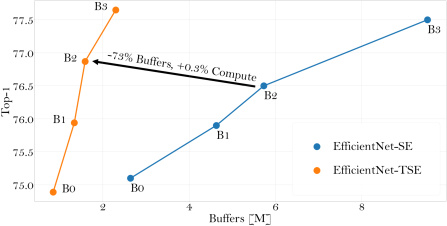
Figure 2: Top-1 accuracy and pipeline memory buffer comparison on ImageNet-1K between different models of EfficientNet [27] using SE and our proposed TSE.

2 Related Work

Squeeze-and-excitation networks [15] are a very popular architectural building block with a simple mechanism for channel attention. To improve the accuracy of the original operation, several works used spatial-attention either in parallel or in series [31, 18, 24, 9]. Recently, TA [21] proposed to attend to each tensor dimension separately and fuse the results. Another line of inquiry is better ways to aggregate the global spatial context [14, 10, 2, 11, 22]. ECANet [29] proposed a more efficient excitation operator using 1D convolutions. Nevertheless, no SE variant has surpassed SE in popularity and use. SE block are an essential building block of many neural architecture searches (NAS) for mobile and edge devices [1, 13, 23, 27]. Specifically, the analysis done in [23] showed that the design space which includes the SE block has higher accuracy models than a comparable design space without it.

Another line of research studied the spatial context required for attention. Non-local network [30] showed that learning long-range dependencies is important for tasks which include a temporal dimension such as video classification. They also showed that long range dependencies are useful for object detection. Further analysis by [2] showed that, in practice, the attended context is position independent and therefore the block can be simplified. Both of these works use global spatial-context. Concurrent to our work, coordinate attention [12] proposed to look at limited spatial context composed of both vertical and horizontal strips. Similarly to us, they limit the amount of spatial context used to strips of one row or column and show that they can match the performance of MobileNetV2 [25] with SE. However, the focus of their work is on improving the accuracy of SE and so they provide no further analysis or experiments on that front.

The work most closely related to ours is the Gather-Excite (GE) framework [14]. The framework introduced in the paper is very suitable for studying the effects of spatial-context on channel attention and with slight modifications to their formulation our block of TSE can be seen as an instantiation of GE. Nonetheless, the focus of their work is how to better encode global spatial-context to get maximal accuracy.

Different from all the above, our work is focused on exploring the amount of spatial context required for effective channel-attention and not on improving the accuracy of the SE operation. Compared with other works, our TSE block relies solely on local spatial context.

3 Tiled Squeeze-and-Excite

In this section, we present tiled squeeze-and-excite, a framework for exploring the amount of spatial context required for effective channel attention. Tiled squeeze-and-excite is a modification of the SE block [15] which preservers the numbers of parameters but enables to vary the spatial-context used. Our goal is to find the minimum spatial context required to match the accuracy achieved with global context.

3.1 Tiled Squeeze

We begin with a review of the original squeeze-and-excite block. Given a tensor of dimensions $T\in\mathbb{R}^{H\times W\times C}$, the squeeze-and-excite operator re-scales each channel by a scalar in the range [0,1]. The ”squeeze” operation is parameter-free and encodes the global spatial context of each channel into a single descriptor by means of global average pooling (GAP). It’s output is a tensor of dimensions $Z\in\mathbb{R}^{1\times 1\times C}$. The ”excite” operation performs channel-attention using a two-layer fully-connected feed-forward network described by $\sigma(W2\cdot ReLU(W_{1}Z))$ where $W_{1}\in\mathbb{R}^{C\times C/r}$, $W_{2}\in\mathbb{R}^{C/r\times C}$ and $\sigma$ denotes the sigmoid activation function. The output of the excite operation is a vector of length $C$ which is than used to scale the channels of the input tensor via element-wise multiplication. Note that the SE block has a built-in separation between spatial-context encoding (squeeze) and channel-attention (excite). Since we are interested in studying the effect of spatial-context encoding without changing the channel-attention mechanism, we keep the excite operation as is. To keep alignment with the original SE block we also wish to avoid adding parameters to the squeeze operation. Thus, what we want is a parameter-free squeeze block whose spatial-context can be varied.

\psfrag{A}[cc][cc][0.8]{$GAP$}\psfrag{B}[cc][cc][0.8]{$FC\,(C\rightarrow C/r)$}\psfrag{C}[cc][cc][0.8]{$ReLU$}\psfrag{D}[cc][cc][0.8]{$FC\,(C/r\rightarrow C)$}\psfrag{E}[cc][cc][0.8]{$Sigmoid$}\psfrag{x}[cl][cc][0.6]{$W\times H\times C$}\psfrag{y}[cl][cc][0.6]{$1\times 1\times C$}\psfrag{z}[cl][cc][0.6]{$1\times 1\times C/r$}\psfrag{w}[cl][cc][0.6]{$1\times 1\times C$}\includegraphics[width=411.93767pt]{SE_block_diagram_4.eps}

(a) SE block

\psfrag{A}[cc][cc][0.8]{$AvgPool\,(h,w/h,w)$}\psfrag{B}[cc][cc][0.8]{$Conv1\times 1\,(C\rightarrow C/r)$}\psfrag{C}[cc][cc][0.8]{$ReLU$}\psfrag{D}[cc][cc][0.8]{$Conv1\times 1\,(C/r\rightarrow C)$}\psfrag{E}[cc][cc][0.8]{$Sigmoid$}\psfrag{F}[cc][cc][0.8]{$Interpolation$}\psfrag{x}[cl][cc][0.6]{$W\times H\times C$}\psfrag{y}[cl][cc][0.6]{$\lceil H/h\rceil\times\lceil W/w\rceil\times C$}\psfrag{z}[cl][cc][0.6]{$\lceil H/h\rceil\times\lceil W/w\rceil\times C/r$}\psfrag{w}[cl][cc][0.6]{$\lceil H/h\rceil\times\lceil W/w\rceil\times C$}\psfrag{t}[cl][cc][0.6]{$W\times H\times C$}\includegraphics[width=411.93767pt]{tSE_block_diagram_4.eps}

(b) Tiled-SE block

Figure 3: Block diagram of the proposed block. (a) The original SE block. (b) the Tiled-SE block. Tiled-SE uses average-pooling with limited extent in-place of the global pooling. The stride of the pool is the same as the kernel dimension so tiles are non-overlapping. Before scaling, the tiles are broadcast back to the dimensions of the input tensor using nearest-neighbour interpolation.

Our proposed concept is as follows: we spatially partition the input tensor to non-overlapping tiles of equal size. The channels of each tile are then re-scaled by SE block which is shared for all tiles. The re-scaled tiles are then stitched back together to get the output tensor. We term this operation - tiled squeeze-and-excite (TSE). Since the channel-attention relies on aggregated spatial context, we expect that as we increase the tile size, the attention mechanism will become more effective and the performance of the network will improve. Tiled-SE is illustrated in Figure 1. The implementation of TSE is simple: To produce tiles, we replace the GAP of the SE block with average pooling with both kernel and stride matching the size of the tile - $AvgPool2D((h,w))$. The number of tiles produced is $N=\lceil\dfrac{H}{h}\times\dfrac{W}{w}\rceil$. The fully-connected layers are changed to 1x1 convolutions. The output of the sigmoid is resized to the dimensions of the input tensor using nearest-neighbour interpolation. A block-diagram of the implementation is shown in Figure 3 and the matching PyTorch code is given in the supplementary material.

We note that it is possible to change many of the design selections made in TSE (see supplementary material for different configuration). Here we opt for the simplest configuration without any bells-and-whistles due to two considerations: (1) we want to isolate the effect of using local-context from any other changes to the architecture and (2) we want to stay compatible with the original SE block. In later sections, we show that the interchangeability of SE and TSE means we can interpret TSE as an estimator of SE (or as a noisy approximation of SE). In our experiments we show that it allows us to plug-in TSE into models trained with SE without re-training.

3.2 TSE Instantiations

Switching from global spatial-context to tiles introduces a new hyper-parameter of tile size. In this section, we study how different tile sizes affect the performance of TSE. We choose to investigate two types of tiling strategies:

1. Strip-tiling in which tiles are composed of $k$ strips of either rows or columns. $k$ is constant across the network. Note that when using strip-tiling the size of the tile (as measured by amount of elements in the tile) decreases as the spatial dimension of the network is decreased but the ratio of tile-size to tensor-size increases since $k$ becomes larger with respect to spatial dimensions of the tensor. We denote by $TSE_{k\times W},TSE_{H\times k}$ row and columns tiles respectively. For simplicity, when discussing strip-tiling in the text we will implicitly mean row-tiling unless explicitly stated otherwise.

2. Patch-tiling in which tiles are composed of fixed-size $k\times k$ patches. $k$ is constant across the network. Note that while the size of the tile remains constant the ratio of tile-size to tensor-size increases as the spatial dimension of the network decreased. We denote by $TSE_{k\times k}$ patch-tiles.

For a given input-tensor a change in tile-size affects three metrics: accuracy, compute and the pipeline buffering. We thoroughly discuss the effect on accuracy as we vary the tile size in Section 3.3. Before that, we briefly review the implications for compute and buffering herein.

\psfrag{A}[cc][cc][1.0]{SE${}_{2,3}$}\psfrag{B}[cc][cc][1.0]{SE${}_{3,4}$}\includegraphics[scale={1.0}]{cor.eps}

Figure 4: Correlation map induced by the squeeze operation (purple) and excite operation (green) at different depths in RegNetY-800MF [23] on ImageNet-1K. On top, stage 2 block 3 and on the bottom stage 3 block 4. The colored dots represents the 50% of the centred tiles. This figure is best viewed in color.

Compute. We denote the additional compute introduced by an individual SE block as $F$. The compute of the corresponding TSE block is therefore $N\cdot F$ where $N$ is the number of tiles used by TSE. Generally speaking, the additional compute introduced by each SE block is small and for strip-tiling the number of tiles $N$ is small (e.g. in the order of few millions FLOPs in EfficientNet-B3) so the overall increase in compute is negligible. However, since the number of tiles scales with input resolution (linearly for strip-tiling and quadratically for patch-tiling), the additional compute may become non-negligible at high-resolutions. From a compute perspective we would rather select large tiles but for most networks the modest additional compute is offset by a significant rise in network accuracy. Therefore, we treat compute as a secondary consideration.

Buffering. As discussed in Section 1, one of the motivations for working with limited spatial-context is to minimize the required pipeline buffering in dataflow architectures [3]. Ignoring implementation details, the minimum buffering required for TSE is $h\times w\times C$, where $h,w$ are the spatial dimensions of the tile. For strip-pooling the amount of required buffering is $k\times W\times C$ and it is linear in both $W$ and $k$. As the input resolution increases so does the amount of required buffering. For patch-tiling the required buffering is $k\times k\times C$ which is quadratic in $k$ but independent of the spatial dimensions of the tensor. The amount of actual buffering required depends on the HW implementation. For example, row-stationary architectures [5, 4] have pipeline-buffering granularity that is $\propto W$ and therefore can benefit most from strip-tiling. From a buffering perspective we would rather select small tiles.

3.3 Local Spatial Context for Channel Attention

As mentioned in section 3.1, TSE is compatible to SE and can therefore be plugged-in instead of SE in a network after it was trained with the SE block. If the local spatial context within each tile is a good estimation of the global spatial context than such a replacement should result in minimum performance degradation. Thus, we treat each tile’s mean as an estimation of the global mean. If we assume that (1) activations are distributed homogeneously across the spatial dimension and (2) that the number of sampling points in each tile is large compared to the variance of the activation, than we are guaranteed (in the mean) to obtain good performance when replacing SE by TSE. More formally, we denote the GAP of channel $i$ as $G_{i}$ and the mean of tile $j$ of the same channel as $T_{i}^{j}=G_{i}+\delta_{i}^{j}$ where the $\delta$ denotes the difference in the mean of the tile compared to the GAP. If we denote the number of points in the tile as $n$ and the variance of the activations in the channel as $\sigma_{i}^{2}$ then $\delta_{i}\propto\sqrt{\sigma_{i}/n}$. Then the scale vector $S^{j}_{i}$ estimated by tile $j$ is given by:

$$S^{j}_{i}=\sigma(W2\cdot ReLU(W_{1}\cdot(G_{i}+\delta^{j}_{i}))$$ (1)

Equation 1 shows that we can treat TSE as a noisy approximation of SE.

Previous works also showed that SE has larger contribution in deeper layers [15, 14]. Therefore, to match the performance of SE, we would want tiles that become progressively larger. This is exactly what TSE achieves: the tile-to-tensor size ratio is increased for deeper layers, making TSE a progressively better estimator. We verify the above analysis by the following experiment: we take a network trained with SE and we replace one of the layers with strip-pooling TSE without retraining. Then we measure the correlation between the GAP of the layers and the means of the tiles. We test the correlation both after the squeeze operation and after the excite operation. We do the experiment with different values of $k$ and we select shallow and deep layers. The results are shown in Figure 4. As expected, the correlation improves as we increase the tile size.

4 Experiments

In this section we first study the impact of different tile sizes in TSE and empirically show the viability of using smaller spatial context to learn meaningful channel attention factors. Next, we evaluate the performance of TSE when used as a replacement in networks pre-trained with SE. These experiments confirms that TSE can be used in existing SE networks without re-training or with a short fine-tuning step. Finally, we report the results of TSE on variety of models in image classification, object detection and semantic segmentation. We show that TSE generalizes across different models, different tasks and a wide scale of input resolutions.

4.1 Implementation Details

We evaluate TSE on ImageNet-1K [7] for image classification, MS COCO [17] for object detection and Cityscapes [6] for semantic segmentation. To make the comparison to SE baseline meaningful, we reproduce all SE results using the same framework as we use for TSE. The image classification models were implemented using the pycls toolkit. Each model was trained with 8 V100 GPUs for 100 epochs using stochastic gradient descent (SGD), momentum of 0.9 and weight decay of 5e-5. The base learning rate was set to 0.8 for the RegNet [23] models and to 0.4 for the EfficientNet [27] models. We follow the cosine learning policy for updating the learning rate during training [19]. Our results were obtained with a short training schedule and without enhancements.

The object detection models were implemented in EfficientDet-PyTorch toolkit and we optimized the models for 300 epochs using an SGD optimizer, momentum of 0.9 and weight decay of 4e-5. The base learning rate was set to 0.08 and we updated it according to the cosine decay method. For augmentation, we only used random flip and resize without special enhancement.

The semantic segmentation models were implemented using the MMSegmenation toolkit. We optimized the models using SGD for 160k iterations with base learning rate of 1e-2, momentum of 0.9 and weight decay of 5e-4.

4.2 Channel Attention with Local Spatial-Context

Here, we examine how the accuracy of the network changes as we vary the tile size in TSE. All experiments are done with the RegNetY-800MF [23] architecture. We make several empirical claims:

Local-context is sufficient. We train the model using three different configurations: strip-tiling of rows (TSE_k×W), strip-tiling of columns (TSE_H×k) and patch-tiling (TSE_k×k). For strip-tiling we vary $k$ from 1 to 9 and for patch-tiling we vary $k$ from 1 to 13 since patch-tiles are smaller than strip-tiles. We compare the results to a baseline when the model is trained with and without SE. The full results are given in Table 1. We see that for all tiling strategies, we are able to match the performance of SE using only a portion of the global spatial context. Thus, we show that effective channel attention does not require global context. For strip-pooling a value of $k=7$ is sufficient to match the accuracy of SE while for patch-pooling $k=13$ is needed in order to be on par. We note that the spatial dimension of the last feature map in our model is $7\times 7$ so for $k=7$ SE and TSE converge.

Method	Params	MFLOPs	Buffer	Top-1
Vanilla	5.4M	796.35	N/A	75.07
SE	6.2M	797.18	1.07M	76.30
TSE7×W-upper	6.2M	797.18	1.07M	75.88
TSE7×W-middle	6.2M	797.18	1.07M	76.25
TSE9×W	6.2M	797.68	0.52M	76.32
TSE7×W	6.2M	797.88	0.42M	76.29
TSE5×W	6.2M	798.49	0.30M	75.98
TSE3×W	6.2M	799.92	0.18M	76.00
TSE1×W	6.2M	807.03	0.06M	75.79
TSEH×9	6.2M	797.68	0.52M	76.49
TSEH×7	6.2M	797.88	0.42M	76.42
TSEH×5	6.2M	798.49	0.30M	76.15
TSEH×3	6.2M	799.92	0.18M	75.74
TSEH×1	6.2M	807.03	0.06M	76.07
TSE13×13	6.2M	797.58	0.58M	76.34
TSE11×11	6.2M	797.83	0.43M	76.15
TSE9×9	6.2M	798.03	0.36M	76.02
TSE7×7	6.2M	799.11	0.22M	76.06
TSE5×5	6.2M	801.76	0.11M	75.80
TSE3×3	6.2M	811.35	0.04M	75.44
TSE1×1	6.2M	931.23	N/A	75.54

Table 1: Comparison of different tiles in TSE on RegNetY-800MF [23] network with ImageNet-1K. TSE_h×w stands for tile size $h\times w$. The buffer column indicates the minimum amount of pipeline buffering required for the op throughout the network as detailed in Section 3.2.

Not all locations are equal. To test whether performance is determined by tile size or tile location, we train two additional variants: TSE_7×W-upper and TSE_7×W-middle. Both variants use a single row strip tile. TSE_7×W-upper always uses the upper seven rows while TSE_7×W-middle always uses a row strip centered around the middle row of the tensor. If tile size would be the only factor determining performance we would expect to see both performing on par. Instead, we see that TSE_7×W-middle far outperforms TSE_7×W-upper and, moreover, it performs on par with the original SE and TSE_7×W suggesting that the center of image holds most of the ’interesting’ spatial context. We note, that in ImageNet most images contain an object located in the center of the image and that the above result depend on the dataset and task.

\psfrag{A}[cc][cc][0.5]{TSE${}_{k\times W}$}\psfrag{B}[cc][cc][0.5]{TSE${}_{H\times k}$}\psfrag{C}[cc][cc][0.5]{TSE${}_{k\times k}$}\includegraphics[scale={0.125}]{pool.eps}

(a) With Training

\psfrag{A}[cc][cc][0.5]{TSE${}_{k\times W}$}\psfrag{B}[cc][cc][0.5]{TSE${}_{H\times k}$}\psfrag{C}[cc][cc][0.5]{TSE${}_{k\times k}$}\includegraphics[scale={0.125}]{pool_assign.eps}

(b) Without Training

Figure 5: Pooling tile trends in TSE on ImageNet-1K. In TSE_k×W and TSE_H×k we change the pooling kernel by increasing one dimension and fixing the other and in TSE_k×k we change both spatial dimensions.

The learned channel-attention is a function of tile size: In section 3.3 it was noted that when replacing SE with TSE without training the performance of the network should degrade only slightly if the tile sizes are large enough. A different way to phrase it is that the channel attention learned with global spatial context will also work for local-context, provided that the local context is large enough. In Figure 5, we plot the network accuracy as function of tile size under two scenarios: training the network with TSE from scratch and training the network with SE and post-training replacing the SE with TSE. We see two interesting phenomena. For both strip and patch tiles of size $k=7$ the local-context are good enough estimators of the global spatial context. On the other hand for smaller values of $k$ we see a significant degradation of the results when trying to apply channel-attention learned from global-context to local-context. However, when training from scratch with TSE we see that some channel-attention can be learned even without any context (e.g. TSE_1,1) and the accuracy improves over the baseline model trained without any spatial context. This suggests that for small tiles the channel-attention is different that the one learned when global-context is available.

In all the following sections we adopt a single TSE variant - TSE_7×W - and perform all subsequent experiment only with it.

4.3 Using Pre-Trained Weights

In this section, we evaluate on a wide variety of networks the performance of TSE_7×W when used as a post-training replacement of SE. We adopt the EfficientNet [27] and RegNet [23] family of models for evaluation. The results are presented in Table 2. We see that for most networks the degradation is 0.6% or below but some network exhibit higher degradation. To get some better insight, we take EfficientNet-B3 and RegNetY-3.2GF, the models with the highest degradation in each family, and give a full breakdown of the degradation in each. For this experiment, we only replace part of the SE blocks with TSE and measure degradation. Results are presented in Table 3. We see that degradation is additive and that it mostly arises at later stages of the network. Additionally, in the first stages of the network we can employ TSE blocks with almost zero degradation despite being spatially larger which suggests earlier stages don’t require global spatial context. This confirms previous findings [15, 14] that channel attention is more valuable for deeper layers.

Model	Input	SE	TSE${}_{7\times W}^{aw}$	TSE${}_{7\times W}^{ft}$
RegNetY-200MF	224$\times$224	70.3	70.1(0.2)	70.13(0.16)
RegNetY-400MF	224$\times$224	74.1	73.7(0.6)	73.94(0.16)
RegNetY-600MF	224$\times$224	75.5	75.1(0.4)	75.23(0.27)
RegNetY-800MF	224$\times$224	76.3	75.7(0.6)	75.96(0.34)
RegNetY-1.6GF	224$\times$224	77.9	77.6(0.3)	77.60(0.30)
RegNetY-3.2GF	224$\times$224	78.9	78.2(0.7)	78.77(0.13)
EfficientNet-B0	224$\times$224	75.1	74.6(0.43)	74.96(0.14)
EfficientNet-B1	240$\times$240	75.9	75.1(0.80)	75.72(0.18)
EfficientNet-B2	260$\times$260	76.5	75.5(0.92)	76.20(0.30)
EfficientNet-B3	300$\times$300	77.5	76.3(1.14)	77.14(0.36)

Table 2: Comparing Top-1 accuracy of TSE networks with pre-trained weights of SE on ImageNet-1K. The results for TSE${}_{7\times W}^{aw}$ are obtained by assigning all the weights from the SE network into the TSE_7×W (without training) and TSE${}_{7\times W}^{ft}$ is the same network after fine-tuning. Degradation compared to SE baseline is noted in parenthesis.

Next, we wish to see if performance can be regained by doing a short fine-tuning step. Post TSE replacement, we train the networks a further 40 epochs on a subset of 10% of the ImageNet-1K training data. Results are given in Table 2. We see that after fine-tuning, all the models converged to the baseline result with a small degradation (less than 0.4%). Taken together, these experiments validate that TSE can be used as a post-training replacement for SE. A practical implication is that an SE network can be trained once and deployed on different types of hardware.

Stage	EfficientNet-B3	RegNetY-3.2GF
Baseline	77.5	78.9
Stage-1	77.39(0.11)	78.9(0.00)
Stage-2	77.42(0.08)	78.84(0.06)
Stage-3	77.50(0.00)	78.39(0.51)
Stage-4	77.39(0.11)	78.9(0.00)
Stage-5	77.48(0.02)	-
Stage-6	77.20(0.30)	-
Stage-7	77.01(0.49)	-
TSEaw	76.36	78.2

Table 3: Top-1 degradation breakdown of assigning SE weights into a TSE in different networks on ImageNet-1K. In each stage we replace all the SE blocks with TSE and measure the degradation. The stage terminology is takes from the respective family architectures.

4.4 Training with TSE

In the previous section we validated the performance of TSE when used as post-training replacement for SE. In the following sections we evaluate the performance of the TSE block when the network is trained from scratch with TSE.

4.4.1 Classification

We perform ImageNet-1K classification experiments to evaluate the TSE block compared to SE. Specifically, we follow the same protocol as specified in Section 4.1 and employ TSE_7×W to verify the accuracy gain is maintained across different architectures. Table 4 summarizes the experimental results. For all networks examined, TSE has comparable accuracy with models trained with SE. With respect to the results in section 4.3 we note that training from scratch with TSE gives slightly better results than fine-tuning on networks pre-trained on SE.

Model	SE			TSE7×W
	Top-1	Buffer	GFLOPs	Top-1	Buffer	GFLOPs
RegNetY-200MF	70.3	0.38M	0.2	70.53	0.20M	0.2
RegNetY-400MF	74.1	0.76M	0.4	73.87	0.33M	0.4
RegNetY-600MF	75.5	0.88M	0.6	75.43	0.37M	0.6
RegNetY-800MF	76.3	1.07M	0.8	76.29	0.42M	0.8
RegNetY-1.6GF	77.9	2.07M	1.6	77.87	0.82M	1.6
RegNetY-3.2GF	78.9	2.84M	3.2	78.77	1.07M	3.2
EfficientNet-B0	75.1	2.64M	0.4	74.89	0.85M	0.4
EfficientNet-B1	75.9	4.63M	0.7	75.94	1.34M	0.7
EfficientNet-B2	76.5	5.73M	1.0	76.87	1.59M	1.0
EfficientNet-B3	77.5	9.52M	1.8	77.65	2.30M	1.8

Table 4: Comparison of Top-1 accuracy results on ImageNet-1K for different EfficientNet [27] and RegNetY [23] models .

4.4.2 Object Detection

We evaluate TSE on object detection trained on COCO 2017 [17]. We employ EfficientDet [28] models which are a strong baseline for object detection with extensive usage of SE blocks. Table 5 shows that EfficientDet-TSE has comparable accuracy to SE. We make two important observations. Up-until now, we showed that TSE is comparable to SE at low resolutions only, and since spatial-context is intimately related to input resolution it is not given that TSE’s performance would scale with resolution. Second, object-detection is a much more spatially-sensitive task compared with classification. Thus, we see that our previous conclusion about local spatial-context being sufficient generalize broadly. We also note that at higher resolutions the cost of pipeline-buffering becomes much more prohibitive and here TSE requires $\times$10 less pipeline buffering compared to SE.

		EfficientDet-D0	EfficientDet-D1	EfficientDet-D2
SE	mAP	33.8	39.0	42.3
	Buffer	13.8M	33.6M	50.8
	GFLOPs	2.5	6.1	11
TSE7×W	mAP	33.9	39.6	42.3
	Buffer	1.9M	3.6M	4.7M
	GFLOPs	2.5	6.1	11
TSE${}_{7\times W}^{aw}$	mAP	33.0	38.0	41.0
	Buffer	1.9M	3.6M	4.7M
	GFLOPs	2.5	6.1	11

Table 5: Comparison of mAP accuracy results on MS COCO-2017 validation set for different EfficientDet models [28].

4.4.3 Semantic Segmentation

We evaluate TSE on semantic segmentation trained on Cityscapes [6]. We use MobileNetV3 with an LR-ASPP segmentation head [13] as our comparison model. We conduct the experiments with metric mIoU [8], and only exploit the ’fine’ annotations in the Cityscapes dataset. Models are evaluated with a single-scale of 1024$\times$2048 input on the Cityscapes validation set. Results are shown in Table 6. As for object detection, we note both the very high resolution which this network operates and the spatially-sensitive nature of the task. We see that using strip pooling of only seven rows is still enough to capture the required spatial-context for channel attention.

		MobileNetV3-L	MobileNetV3-S
SE	mIoU	69.54	64.11
	Buffer	36.17M	24.51M
	GFLOPs	68.6	33.5
TSE7×W	mIoU	69.2	63.83
	Buffer	1.59M	1.04M
	GFLOPs	68.6	33.5
TSE${}_{7\times W}^{aw}$	mIoU	69.02	63.83
	Buffer	1.59M	1.04M
	GFLOPs	68.6	33.5

Table 6: Comparison of mIoU accuracy results on Cityscapes validation set for different MobileNetV3 models [13].

5 Conclusion

We have presented the tiled squeeze-and-excite (TSE), a new framework for channel attention that relies on non-overlapping tiles with limited spatial extent. Through analysis and comprehensive experimentation, we have shown that channel-attention learned with local spatial context is equal in performance to attention learned with global-context. We further showed that for large tiles the local-context is a good enough estimator of the global context and therefore TSE can replace SE post-training. Furthermore, TSE significantly reduces the pipeline-buffering requirements in dataflow AI accelerators while preserving baseline accuracy. We hope that our analysis and results will be an important step towards quantifying the importance of spatial context for other attention mechanisms in the future.

Appendix: Tiled Squeeze-and-Excite

Appendix A TSE Code

An implementation in PyTorch of the TSE block is given in Figure A1.

⬇

def TSE(x, kernel, se_ratio):

# x: input feature map [N, C, H, W]

# kernel: tile size (Kh, Kw)

# se_ratio: SE channel reduction ratio

N, C, H, W = x.size()

# tiled squeeze

sq = nn.AvgPool2d(kernel, stride=kernel, ceil_mode=True)

# original se excitation

ex = nn.Sequential(

nn.Conv2d(C, C // se_ratio, 1),

nn.ReLU(inplace=True),

nn.Conv2d(C // se_ratio, C, 1),

nn.Sigmoid()

)

y = ex(sq(x))

# nearest neighbor interpolation

y = torch.repeat_interleave(y, kernel[0], dim=-2)[:,:,:H,:]

y = torch.repeat_interleave(y, kernel[1], dim=-1)[:,:,:,:W]

return x * y

Figure A1: PyTorch code of our TSE block

Appendix B Different Design Selections

Here, we introduce different design selections for TSE that minimize the spatial context of the operation without losing accuracy. We will focus on two different modifications: (a) change the channel reduction ratio, and (b) change the 1x1 convolutions of the excitation step to different operations, e.g., 3x3 convolution. We note that those alteration change the number of parameters in the model and thus make it incompatible with standard SE block. The target of this experiment is to examine whether a model with single row strip pooling or without any pooling can achieve the same accuracy as SE network with GAP.

Method	Params	GFLOPs	Buffer	Top-1
SE	6.2M	0.79	1.07M	76.30
TSE${}_{1\times W}C_{1\times 1}R_{4}$	6.2M	0.80	0.06M	75.79
TSE${}_{1\times W}C_{1\times 1}R_{2}$	7.08M	0.81	0.06M	75.90
TSE${}_{1\times W}C_{3\times 1}R_{4}$	7.8M	0.82	0.06M	76.40
TSE${}_{1\times W}C_{3\times 1}R_{2}$	10.3M	0.84	0.06M	76.43
TSE${}_{1\times 1}C_{1\times 1}R_{4}$	6.2M	0.93	-	75.54
TSE${}_{1\times 1}C_{1\times 1}R_{2}$	7.08M	2.84	-	75.90
TSE${}_{1\times 1}C_{3\times 3}R_{2}$	20.17M	2.84	-	77.14

Table B1: Different design selections for TSE. Top-1 accuracy comparison of different RegNetY-800MF models on ImageNet-1K. The naming convention is: TSE${}_{h\times w}C_{k_{x}\times k_{y}}R_{c}$ where $C_{k_{x}\times k_{y}}$ and $R_{c}$ are the dimensions of the convolution kernel and the channel reduction ratio, respectively.

We consider two operations to swap the 1x1 convolution with: $Conv2D_{3\times 3}$ and $Conv2D_{3\times 1}$ and each model is named according to the following scheme: TSE${}_{h\times w}C_{k_{x}\times k_{y}}R_{c}$ where $C_{k_{x}\times k_{y}}$ and $R_{c}$ are the dimensions of the convolution kernel and the channel reduction ratio, respectively. For instance, TSE${}_{1\times W}C_{3\times 1}R_{2}$ is a model with strip pooling of a single row, channel reduction ratio of $2$ and two $Conv2D_{3\times 1}$ operations. The baseline in our experiment is RegNetY-800MF model [23] which has a native channel reduction ratio of $4$. The results are shown in Table B1.

Model	Input	SE			TSE1×W
		mAP	Buffer	GFLOPs	mAP	Buffer	GFLOPs
EfficientDet-D0	512$\times$512	33.8	13.8M	2.5	34.4	0.28M	2.7
EfficientDet-D1	640$\times$640	39.0	33.6M	6.1	39.5	0.52M	6.7
EfficientDet-D2	768$\times$768	42.3	50.8M	11	42.4	0.68M	11.8

Table B2: Comparison of mAP accuracy results on MS COCO-2017 validation set for different EfficientDet models [28] with TSE${}_{1\times w}C_{3\times 1}R_{4}$.

TSE Without Pooling. In the first experiment we use TSE without pooling, e.g., TSE_1×1 (bottom part of Table B1). The baseline top-1 accuracy of 75.54% obtained with the original excitation step of SENet and without any pooling. First, we show that decreasing the channel reduction ratio can increase the accuracy of the network by 0.36%. However, even with reduction ratio of $2$ the network has a large accuracy margin compare to the SE model. Second, we replace the $Conv2D_{1\times 1}$ operation with $Conv2D_{3\times 3}$. This replacement increases the number of parameters and compute but also improves network accuracy above the SE baseline. The purpose of this experiment is to show that GAP (or any global spatial context) is not mandatory for channel attention and variations in the excitation step can ’overcome’ the lack of spatial context and even give improvement over more basic excitation schemes with global pooling. It also shows the trade-off between the number of parameters and compute to pipeline buffering which optimally can be optimized to a specific hardware.

Single Row Strip-tiling. Here, we use TSE with a single row strip-tiling, e.g., TSE_1×W. Unlike the first experiment, here, we squeeze the rows which induces less computation. We also note that changing the channel reduction ratio has limited accuracy gains. To match SE accuracy in this case, we swap the $Conv2D_{1\times 1}$ convolution to $Conv2D_{3\times 1}$ which increases the number of parameters (even with the same channel reduction ratio). This variant of TSE shows how minimum amount of spatial context can be enough to generate meaningful attention factors. We further verified that TSE${}_{1\times W}C_{3\times 1}R_{4}$ can be used with high resolution networks as well. For this experiment, we employ the EfficientDet [28] models. The results are shown in Table B2 and shows that the same accuracy can be achieved with less pipeline buffering with the cost of adding a small amount of additional computations.

In summary, both experiments show that there is a rather large design space for SE-like operations. Spatial squeezing has a dual role of decreasing computation and aggregating spatial context, however, the more spatial information is squeezed, the greater the buffering required. At the extreme, spatial squeezing can be avoided altogether with the cost of increased computations and reduced accuracy. Adding a spatial component to the excite operation improves the performance of channel attention while significantly increasing the number of parameters. In fact, using $Conv2D_{3\times 3}$ has superior performance than the original SE block. The original SE block uses GAP to reduce the compute to minimum and a simple excitation to reduce the parameter count to a minimum, however, is also maximizes the required pipeline buffering. Based on the above observations, TSE is designed to bring all three of compute, parameters and buffering to a minimum while maintaining accuracy.

References

- [1] Han Cai, Chuang Gan, Tianzhe Wang, Zhekai Zhang, and Song Han. Once-for-all: Train one network and specialize it for efficient deployment. In ICLR, 2020.
- [2] Yue Cao, Jiarui Xu, Stephen Lin, Fangyun Wei, and Han Hu. Gcnet: Non-local networks meet squeeze-excitation networks and beyond. In ICCV, 2019.
- [3] Yiran Chen, Yuan Xie, Linghao Song, Fan Chen, and Tianqi Tang. A survey of accelerator architectures for deep neural networks. In Engineering, 2020.
- [4] Yu-Hsin Chen, Joel Emer, and Vivienne Sze. Eyeriss: A spatial architecture for energy-efficient dataflow for convolutional neural networks. In ISCA, 2016.
- [5] Yu-Hsin Chen, Tushar Krishna, Joel S. Emer, and Vivienne Sze. Eyeriss: An energy-efficient reconfigurable accelerator for deep convolutional neural networks. In IEEE Journal of Solid-State Circuits, 2017.
- [6] Marius Cordts, Mohamed Omran, Sebastian Ramos, Timo Rehfeld, Markus Enzweiler, Rodrigo Benenson, Uwe Franke, Stefan Roth, and Bernt Schiele. The cityscapes dataset for semantic urban scene understanding. In CVPR, 2016.
- [7] Jia Deng, Wei Dong, Richard Socher, Li-Jia Li, Kai Li, and Li Fei-Fei. Imagenet: A large-scale hierarchical image database. In CVPR, 2009.
- [8] Mark Everingham, S. M. Ali Eslami, Luc Van Gool, Christopher K. I. Williams, John Winn, and Andrew Zisserman. The pascal visual object classes challenge: A retrospective. In International Journal of Computer Vision, 2014.
- [9] Jun Fu, Jing Liu, Haijie Tian, Yong Li, Yongjun Bao, Zhiwei Fang, and Hanqing Lu. Dual attention network for scene segmentation. In CVPR, 2019.
- [10] Zilin Gao, Jiangtao Xie, Qilong Wang, and Peihua Li. Global second-order pooling convolutional networks. In CVPR, 2019.
- [11] Qibin Hou, Li Zhang, Ming-Ming Cheng, and Jiashi Feng. Strip pooling: Rethinking spatial pooling for scene parsing, 2020.
- [12] Qibin Hou, Daquan Zhou, and Jiashi Feng. Coordinate attention for efficient mobile network design, 2021.
- [13] Andrew Howard, Mark Sandler, Grace Chu, Liang-Chieh Chen, Bo Chen, Mingxing Tan, Weijun Wang, Yukun Zhu, Ruoming Pang, Vijay Vasudevan, Quoc V. Le, and Hartwig Adam. Searching for mobilenetv3. In ICCV, 2019.
- [14] Jie Hu, Li Shen, Samuel Albanie, Gang Sun, and Andrea Vedaldi. Gather-excite: Exploiting feature context in convolutional neural networks. In NeurIPS, 2018.
- [15] Jie Hu, Li Shen, and Gang Sun. Squeeze-and-Excitation networks. In CVPR, June 2018.
- [16] Youngwan Lee and Jongyoul Park. Centermask : Real-time anchor-free instance segmentation. In CVPR, 2020.
- [17] Tsung-Yi Lin, Michael Maire, Serge Belongie, Lubomir Bourdev, Ross Girshick, James Hays, Pietro Perona, Deva Ramanan, C. Lawrence Zitnick, and Piotr Dollár. Microsoft coco: Common objects in context. In ECCV, 2014.
- [18] Drew Linsley, Dan Shiebler, Sven Eberhardt, and Thomas Serre. Learning what and where to attend, 2019.
- [19] Ilya Loshchilov and Frank Hutter. Sgdr: Stochastic gradient descent with warm restarts. In ICLR, 2017.
- [20] Ningning Ma, Xiangyu Zhang, Hai-Tao Zheng, and Jian Sun. Shufflenet v2: Practical guidelines for efficient cnn architecture design. In ECCV, 2018.
- [21] Diganta Misra, Trikay Nalamada, Ajay Uppili Arasanipalai, and Qibin Hou. Rotate to attend: Convolutional triplet attention module, 2020.
- [22] Zequn Qin, Pengyi Zhang, Fei Wu, and Xi Li. Fcanet: Frequency channel attention networks, 2021.
- [23] Ilija Radosavovic, Raj Prateek Kosaraju, Ross Girshick, Kaiming He, and Piotr Dollár. Designing network design spaces. In CVPR, 2020.
- [24] Abhijit Guha Roy, Nassir Navab, and Christian Wachinger. Recalibrating fully convolutional networks with spatial and channel ‘squeeze & excitation’ blocks. In IEEE TRANSACTIONS ON MEDICAL IMAGING, 2018.
- [25] Mark Sandler, Andrew Howard, Menglong Zhu, Andrey Zhmoginov, and Liang-Chieh Chen. Mobilenetv2: Inverted residuals and linear bottlenecks, 2019.
- [26] Mingxing Tan, Bo Chen, Ruoming Pang, Vijay Vasudevan, Mark Sandler, Andrew Howard, and Quoc V. Le. Mnasnet: Platform-aware neural architecture search for mobile. In CVPR, 2019.
- [27] Mingxing Tan and Quoc V. Le. Efficientnet: Rethinking model scaling for convolutional neural networks. In ICML, 2019.
- [28] Mingxing Tan, Ruoming Pang, and Quoc V. Le. Efficientdet: Scalable and efficient object detection. In CVPR, 2020.
- [29] Qilong Wang, Banggu Wu, Pengfei Zhu, Peihua Li, Wangmeng Zuo, and Qinghua Hu. ECA-Net: Efficient channel attention for deep convolutional neural networks. In CVPR, June 2020.
- [30] Xiaolong Wang, Ross Girshick, Abhinav Gupta, and Kaiming He. Non-local neural networks. In CVPR, 2018.
- [31] Sanghyun Woo, Jongchan Park, Joon-Young Lee, and In So Kweon. CBAM: Convolutional block attention module. In ECCV, September 2018.