Enhanced diffusion in soft-walled channels with a periodically varying curvature
Abstract
In one-dimension, the diffusion of particles along a line is slowed by the addition of energy barriers. The same is true in two-dimensions, provided that the confining channel in which the particles move doesn’t change shape. However, if the shape changes then this is no longer necessarily true; adding energy barriers can enhance the rate of diffusion, and even restore free diffusion. We explore these effects for a channel with a sinusoidally varying curvature.
I Introduction
Transport processes in channels of varying profile have been studied for many years. With applications in disparate fields such as zeolites and porous solids [1, 2], biological membranes [3, 4, 5], separating particles by their size [6, 7, 8] and carbon nanotubes [9], the importance of understanding these systems’ behaviour is clear.
A common starting point is the Fick-Jacobs equation, an effective, one-dimensional equation for the evolution of the concentration of a solute along the centre-line of a multi-dimensional tube. Jacobs’ treatment [10], which he attributed to Fick [11], was refined by Zwanzig [12], who produced a more general version. By assuming that the system is fully equilibrated in the direction normal to the length of the channel, Zwanzig reduced the multi-dimensional Smoluchowski equation to a one-dimensional form with a modified potential. The changing shape of the channel produces a logarithmic contribution to this potential, which leads to the description of the effect upon the motion in terms of ‘entropic’ barriers [13].
However, it isn’t safe to assume that the system equilibrates fully in the confining direction; a shape which varies too rapidly, for instance, can prevent equilibrium from being established [14]. Zwanzig acknowledged the limitations of this approach and suggested how small deviations from equilibrium might be accounted for. This work, based around a spatially varying diffusion coefficient, has been built upon heavily [15, 16, 17, 18].
Introducing a linear bias along a periodic channel leads to motion described by a redefined effective diffusion coefficient and a non-linear mobility. The former peaks for some value of the applied force, before falling to a constant value; the latter increases monotonically towards a constant value [19, 20, 21].
Although channels which are symmetrical about their axis feature prominently in this field, the more general case of a curved midline and varying width has also attracted attention. The motion can still be mapped onto one dimension, albeit with a modified expression for the spatially varying diffusion coefficient, which now reflects the variation in the midline of the channel [22, 23, 24, 25]. Motion in serpentine channels, where the midline is curved but the width is constant, has also been studied [26, 27].
Channels of curved midline and varying width can be created by using the same function to describe both walls, but then introducing a phase difference between the two. The current can be affected by this phase shift and a preferential direction of transport can emerge [28, 29].
Adding potential energy barriers to a channel of varying width can cause interesting effects because of the interaction between the energetic and entropic contributions to the potential. For instance, introducing a linear bias along the channel and tuning the phase difference between the periodic channel and the periodic barriers can induce a resonance-like behaviour in the non-linear mobility, and rectification can be observed [30]. Another example involves a channel with cosine-shaped walls which connects two reservoirs of particles at different concentrations over one period. By introducing a cosine energy barrier along the channel, and tuning the phase relative to the walls, it is possible to produce transport from low to high concentration [31].
Here we study over-damped motion in a soft-walled channel whose profile varies periodically. By introducing a periodic potential along the channel it is possible to increase the rate of diffusion above that observed without the potential, in some cases up to free diffusion. The energy barriers enhance the motion.
II A one-dimensional model for the effective diffusion coefficient
We will consider motion in a channel
| (1) |
where is the potential energy contribution along the channel and describes how the profile of the channel varies as a function of the displacement along it. If the channel is periodic in , then the long-time motion will be diffusive, and so described by an effective diffusion coefficient . We will use Zwanzig’s derivation of the Fick-Jacobs equation to explore the system’s behaviour.
Zwanzig restricted his attention to the effect upon the diffusion coefficient of changes in the shape of the channel [12]. Here we will retain the effect of energy barriers. Our starting point is the two-dimensional Smoluchowski equation for the probability density
| (2) |
where and are the free diffusion coefficients in the and directions, respectively. By inserting Eq. (1) into Eq. (2), integrating over the -direction, and using the fact that is confining, we obtain
| (3) |
where is the one-dimensional probability density. Let us assume that the distribution is always in equilibrium in the -direction, i.e.
| (4) |
where is defined through
| (5) |
Inserting Eq. (4) into Eq. (3) and carrying out the integration over produces the following partial differential equation for the one-dimensional density
| (6) |
from which we can deduce the following expression for the one-dimensional effective potential
| (7) |
Before we restrict our attention to a particular channel it is worth remarking upon an implication of Eq. (7). Variations in the shape of the channel impede motion, a feature accounted for by the second term in the expression for the effective potential. However, Eq. (7) implies that this retarding effect can be eradicated by introducing a potential in the -direction: by setting the effective potential is zero and free diffusion is predicted. This is a point to which we will return.
We will now focus on the potential energy landscape
| (8) |
where , and to make the channel confining, and study the effects of and on the motion.
With the expression for the one-dimensional effective potential in Eq. (7), we can derive the effective diffusion coefficient by considering the mean first-passage time from the potential energy maximum at to either of the maxima at . This is given by
| (9) |
where and are the probabilities that the particle exits the region to the left and right, respectively [32]. The symmetry of the energy landscape means that , and Eq. (9) simplifies to
| (10) |
where we have used the periodicity of the potential to recast each integral over one period.
After evaluating Eq. (7) for the potential defined in Eq. (8), inserting the result into Eq. (10), and changing variables to , we find
| (11) |
where the quantities are given by
| (12) |
and is the phase difference. Finally, we obtain the effective diffusion coefficient
| (13) |
The derivative of with respect to can be an informative quantity. For a one-dimensional system it is at most zero, and it is negative for ; increasing the height of the energy barriers reduces the size of the effective diffusion coefficient. Our quasi-one-dimensional system displays a more complicated behaviour:
| (14) |
where , and is a positive constant given by
| (15) |
A central result of our work is that Eq. (14) can be positive; adding energy barriers can enhance the rate of diffusion along the channel.
III Brownian dynamics simulations
We used numerical simulations to study the two aspects of this work: the effect of the phase difference upon the behaviour of the effective diffusion coefficient, and the exact cancellation of energetic and entropic barriers to motion. Unless stated otherwise, simulations were performed with particles, a time step units, and unit values of the thermal energy and damping coefficients and .
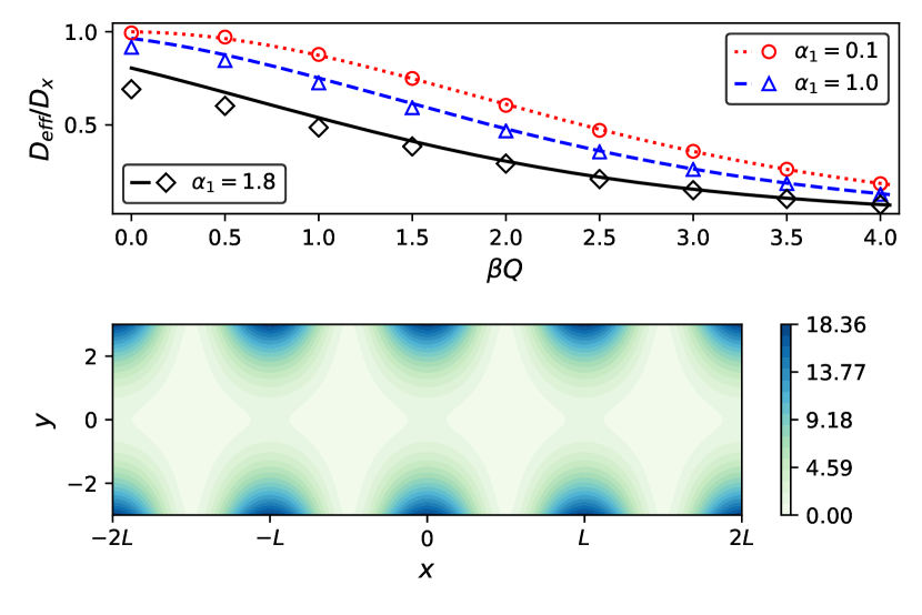
Eq. (14) predicts that the gradient of the effective diffusion coefficient at is proportional to . We performed simulations for and to investigate the extremal cases. We will start with the former, because the behaviour is familiar.
We expect a negative gradient at , and hence a monotonically decreasing effective diffusion coefficient. Fig. (1) confirms these expectations and reveals good agreement between theory and simulations over a range of amplitudes. This is because the potential energy minima – around which the particles spend the bulk of their time – coincide with the points of minimum curvature. The distribution can get closer to its equilibrium shape in the regions of the channel where it would otherwise struggle most to do so. Agreement improves with increasing amplitude because more time is spent around the minima. Finally, agreement is better for smaller values of because the variations in curvature are smaller.
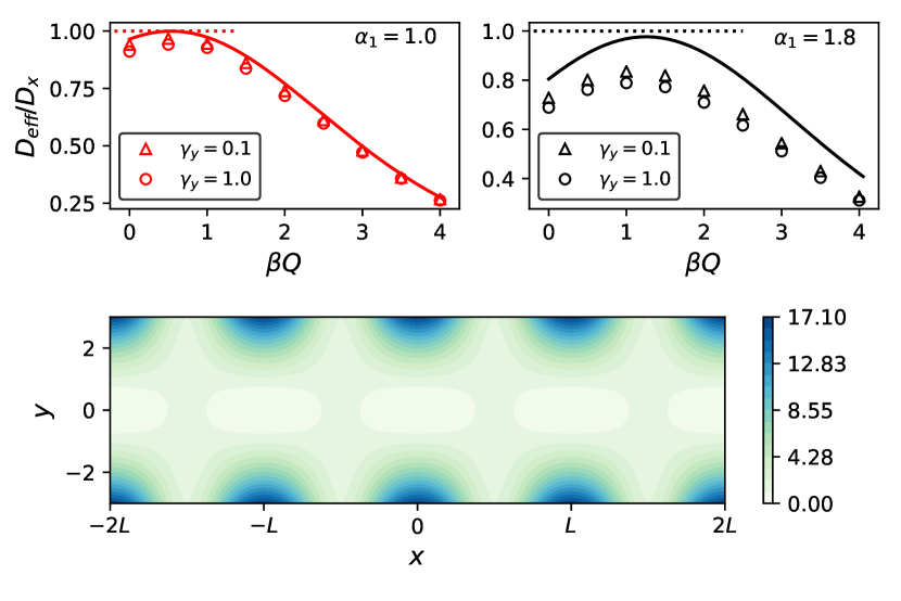
Let us now turn to the case . Eq. (14) predicts that the effective diffusion coefficient initially grows with the amplitude of the potential energy barriers. Fig. (2) confirms this and reveals qualitative agreement between theory and simulations. However, quantitative agreement is not as good as in the previous case. This is because the points of minimum curvature coincide with the potential energy maxima. These are unstable points and particles pass through them quickly, leaving little chance for the ensemble to equilibrate. When we see good quantitative agreement with the theory for values of . In contrast, for there is a lack of good agreement even for . This is because the size of the entropic barriers to motion increases with the variation in the curvature of the channel, which is controlled by . For smaller values of , the rate of diffusion along the channel becomes determined by the height of the potential energy barriers at smaller values of the barrier height. Once in this regime, equilibration is less important for close agreement with the theory. As expected, decreasing improves agreement with the theory.
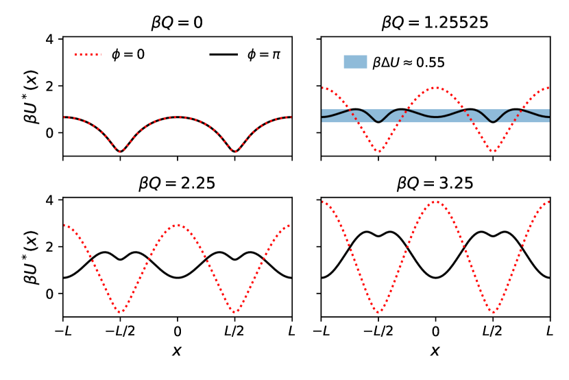
Fig. (3) provides insight into the origin of the behaviour of the effective diffusion coefficient: increasing the amplitude of the cosine potential does not necessarily increase the barrier to motion in the effective potential. The energetic and entropic contributions can interact with one another so as to decrease the barrier to motion, as can be seen by comparing the panels for and , chosen because it is a good approximation to the amplitude which minimises the barrier.
The contour plots in Fig. (1) and Fig. (2) further our understanding of this effect. Fig. (1) reveals that introducing the cosine potential creates near-flat regions which extend away from the centre of the channel. By contrast, the near-flat regions in Fig. (2) extend much further along the line of the channel than away from it. The former will inhibit motion along the channel by enabling particles to move significant distances in unproductive directions. The latter comes close to providing a continuous near-flat region along the line of the channel, which is combined with steeper barriers to motion away from it. The region either side of the centre-line is flatter in Fig. (2) than in Fig. (1), and the saddle points are broader, which is beneficial for transport; it is easier for particles to move from a tighter minimum into a broader saddle than vice versa.
Let us conclude this section by returning to a point made after the introduction of the effective potential in Eq. (7). The potential energy landscape
| (16) |
has been constructed by adding to the term describing the shape of the channel a series of potential energy barriers in the -direction such that the effective potential is exactly zero. This predicts free diffusion.
Motion was simulated for a range of values of for . In each case, the effect of decreasing from one to upon the effective diffusion coefficient was studied. Motion was also simulated in the absence of the energy barriers. The results are shown in Fig. (4).
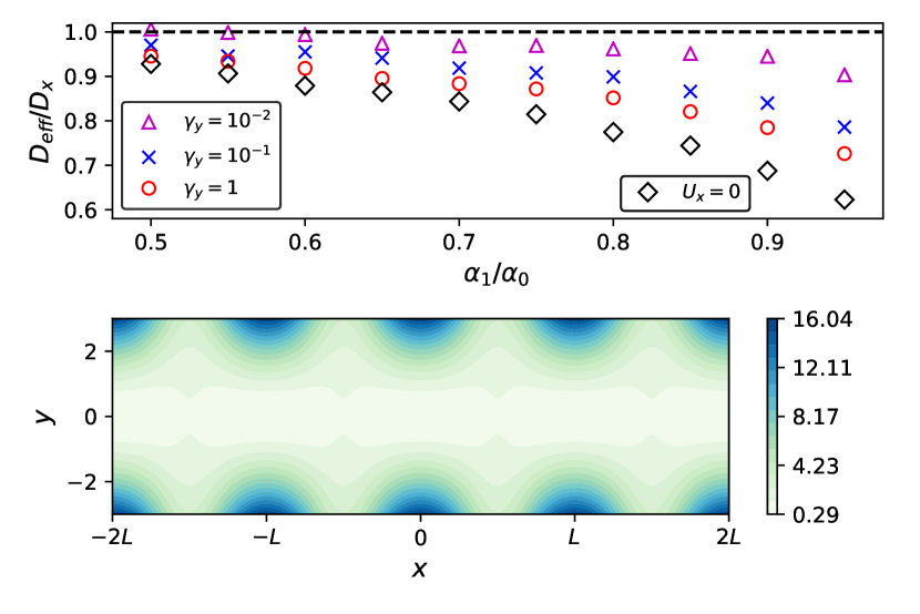
For all values of the effective diffusion coefficient is larger in the presence of energy barriers than in their absence. Again, as expected, decreasing improves agreement with the theory.
IV Conclusions
We used the Fick-Jacobs equation to study the behaviour of particles diffusing along channels with a periodically varying profile and potential energy barriers along their length. Treating the variations in the shape of the channel as entropic barriers to motion reduces the problem to diffusion in an (approximate) one-dimensional potential.
For the cosine-based potential studied here, the position of the potential energy minima relative to the points of minimum curvature determines how the effective diffusion coefficient responds to increasing the height of the energy barriers. If the two coincide, then a monotonic decrease is observed, and there is good quantitative agreement with the theory. If the two are perfectly out-of-phase, so that the energy minima coincide with the regions of maximum curvature, then the effective diffusion coefficient initially increases above its zero-amplitude value, resulting in enhanced diffusion. Good quantitative agreement is observed only when the energy barriers dwarf the entropic barriers. Before this point, lack of equilibration in the confining direction precludes good agreement.
For a given channel it is possible to construct a series of energy barriers which cancel out the entropic barriers; free diffusion is then predicted. Numerical simulations confirm that adding these barriers increases the rate of diffusion, and decreasing the damping coefficient in the confining direction leads ever-closer to free diffusion.
V Acknowledgements
T.H.G acknowledges support from the EPSRC and E.H.Y. acknowledges support from Nanyang Technological University, Singapore, under its Start Up Grant Scheme (04INS000175C230).
References
- Ruthven [1995] D. M. Ruthven, Diffusion in zeolites, in Zeolites: A Refined Tool for Designing Catalytic Sites, Studies in Surface Science and Catalysis, Vol. 97, edited by L. Bonneviot and S. Kaliaguine (Elsevier, 1995) pp. 223–234.
- Schüring et al. [2002] A. Schüring, S. M. Auerbach, S. Fritzsche, and R. Haberlandt, On entropic barriers for diffusion in zeolites: A molecular dynamics study, The Journal of Chemical Physics 116, 10890 (2002).
- Hille [1978] B. Hille, Ionic channels in excitable membranes. current problems and biophysical approaches, Biophysical Journal 22, 283 (1978).
- Berezhkovskii and Bezrukov [2005] A. M. Berezhkovskii and S. M. Bezrukov, Optimizing transport of metabolites through large channels: Molecular sieves with and without binding, Biophysical Journal 88, L17 (2005).
- Liu et al. [1999] L. Liu, P. Li, and S. A. Asher, Entropic trapping of macromolecules by mesoscopic periodic voids in a polymer hydrogel, Nature 397, 141 (1999).
- Corma [1997] A. Corma, From microporous to mesoporous molecular sieve materials and their use in catalysis, Chemical Reviews 97, 2373 (1997), pMID: 11848903.
- Reguera et al. [2012] D. Reguera, A. Luque, P. S. Burada, G. Schmid, J. M. Rubi, and P. Hanggi, Entropic splitter for particle separation, Phys. Rev. Lett. 108, 020604 (2012).
- Motz et al. [2014] T. Motz, G. Schmid, P. Hanggi, D. Reguera, and J. M. Rubi, Optimizing the performance of the entropic splitter for particle separation, The Journal of Chemical Physics 141, 074104 (2014).
- Berezhkovskii and Hummer [2002] A. Berezhkovskii and G. Hummer, Single-file transport of water molecules through a carbon nanotube, Phys. Rev. Lett. 89, 064503 (2002).
- Jacobs [1935] M. H. Jacobs, Diffusion processes, in Diffusion Processes (Springer Berlin Heidelberg, Berlin, Heidelberg, 1935) pp. 1–145.
- Fick [1855] A. Fick, Ueber diffusion, Annalen der Physik 170, 59 (1855).
- Zwanzig [1992] R. Zwanzig, Diffusion past an entropy barrier, The Journal of Physical Chemistry 96, 3926 (1992).
- Reguera and Rubi [2001] D. Reguera and J. M. Rubi, Kinetic equations for diffusion in the presence of entropic barriers, Phys. Rev. E 64, 061106 (2001).
- Gray and Yong [2021] T. H. Gray and E. H. Yong, An effective one-dimensional approach to calculating mean first passage time in multi-dimensional potentials, The Journal of Chemical Physics 154, 084103 (2021).
- Kalinay and Percus [2005] P. Kalinay and J. K. Percus, Projection of two-dimensional diffusion in a narrow channel onto the longitudinal dimension, The Journal of Chemical Physics 122, 204701 (2005).
- Kalinay and Percus [2006] P. Kalinay and J. K. Percus, Corrections to the fick-jacobs equation, Phys. Rev. E 74, 041203 (2006).
- Kalinay and Percus [2008] P. Kalinay and J. K. Percus, Approximations of the generalized fick-jacobs equation, Phys. Rev. E 78, 021103 (2008).
- Burada et al. [2008] P. Burada, G. Schmid, P. Talkner, P. Hanggi, D. Reguera, and J. Rubi, Entropic particle transport in periodic channels, Biosystems 93, 16 (2008).
- Reimann et al. [2002] P. Reimann, C. Van den Broeck, H. Linke, P. Hanggi, J. M. Rubi, and A. Pérez-Madrid, Diffusion in tilted periodic potentials: Enhancement, universality, and scaling, Phys. Rev. E 65, 031104 (2002).
- Reguera et al. [2006] D. Reguera, G. Schmid, P. S. Burada, J. M. Rubi, P. Reimann, and P. Hanggi, Entropic transport: Kinetics, scaling, and control mechanisms, Phys. Rev. Lett. 96, 130603 (2006).
- Burada et al. [2007] P. S. Burada, G. Schmid, D. Reguera, J. M. Rubi, and P. Hanggi, Biased diffusion in confined media: Test of the fick-jacobs approximation and validity criteria, Phys. Rev. E 75, 051111 (2007).
- Bradley [2009] R. M. Bradley, Diffusion in a two-dimensional channel with curved midline and varying width: Reduction to an effective one-dimensional description, Phys. Rev. E 80, 061142 (2009).
- Berezhkovskii and Szabo [2011] A. Berezhkovskii and A. Szabo, Time scale separation leads to position-dependent diffusion along a slow coordinate, The Journal of Chemical Physics 135, 074108 (2011).
- Dagdug and Pineda [2012] L. Dagdug and I. Pineda, Projection of two-dimensional diffusion in a curved midline and narrow varying width channel onto the longitudinal dimension, The Journal of Chemical Physics 137, 024107 (2012).
- Chavez et al. [2018] Y. Chavez, G. Chacon-Acosta, and L. Dagdug, Effects of curved midline and varying width on the description of the effective diffusivity of brownian particles, Journal of Physics: Condensed Matter 30, 194001 (2018).
- Wang and Drazer [2015] X. Wang and G. Drazer, Transport of brownian particles in a narrow, slowly varying serpentine channel, The Journal of Chemical Physics 142, 154114 (2015).
- Wang [2016] X. Wang, Biased transport of brownian particles in a weakly corrugated serpentine channel, The Journal of Chemical Physics 144, 044101 (2016).
- Li and Ai [2013] F.-g. Li and B.-q. Ai, Current control in a two-dimensional channel with nonstraight midline and varying width, Phys. Rev. E 87, 062128 (2013).
- Alvarez-Ramirez et al. [2014] J. Alvarez-Ramirez, L. Dagdug, and L. Inzunza, Asymmetric brownian transport in a family of corrugated two-dimensional channels, Physica A: Statistical Mechanics and its Applications 410, 319 (2014).
- Burada et al. [2010] P. Burada, Y. Li, W. Riefler, and G. Schmid, Entropic transport in energetic potentials, Chemical Physics 375, 514 (2010), stochastic processes in Physics and Chemistry (in honor of Peter Hanggi).
- Zheng et al. [2013] X.-T. Zheng, J.-C. Wu, B.-Q. Ai, and F.-G. Li, Brownian pump induced by the phase difference between the potential and the entropic barrier, The European Physical Journal B 86, 479 (2013).
- Gardiner [2004] C. Gardiner, Handbook of Stochastic Methods for Physics, Chemistry, and the Natural Sciences, Springer complexity (Springer, 2004).