A System Model-Based Approach for the Control of Power Park Modules for Grid Voltage and Frequency Services

Abstract

A new control approach is proposed for the grid insertion of Power Park Modules (PPMs). It allows full participation of these modules to ancillary services. This means that, not only their control have some positive impact on the grid frequency and voltage dynamics, but they can effectively participate to existing primary and secondary control loops together with the classic thermal/inertia synchronous generators and fulfill the same specifications both from the control and contractual points of view.

To achieve such level of performances, a system approach based on an innovatory control model is proposed. The latter control model drops classic hypothesis for separation of voltage and frequency dynamics used till now in order to gather these dynamics into a small size model.

From the system point of view, dynamics are grouped by time-scales of phenomena in the proposed control model. This results in more performant controls in comparison to classic approaches which orient controls to physical actuators (control of grid side converter and of generator side converter). Also, this allows coordination between control of converters and generator or, in case of multimachines specifications, among several PPMs.

From the control synthesis point of view, classic robust approaches are used (like, e.g., H-infinity synthesis).

Implementation and validation tests are presented for wind PPMs but the approach holds for any other type of PPM.

These results will be further used to control the units of the new concept of Dynamic Virtual Power Plant introduced in the H2020 POSYTYF project.

Renewable energy, Power Park Modules, PMSG, MPPT, $H_{\infty}$, RoCoF, Frequency support, droop control, LMI, mixed sensibility, loop-shaping.

1 Introduction

Rapid development of Renewable Energy Sources (RES) brought the concept of Power Park Modules (PPMs) [1]. Indeed, RES, like, e.g., solar and wind [2] are systematically connected to the grid via power electronics (like back-to-back power converter structures) (e.g., [2], [3]).

PPMs and, generally, power electronics bring fast dynamics into power systems [4]. Also, compared with dynamics of classic synchronous thermal generators, voltage and power dynamics are coupled in the same range of frequency. Old hypothesis and way of doing which separate control of voltage and power tracks should be revisited into more coordinated controls which need new concepts of modeling and regulation.

Massive integration of RES lowers also the global inertia of the power system [3], [4]. The Rate of Change of Frequency (RoCoF) is increased [5], [6] which results in a need for fast frequency support from RES. Several approaches dealt with this as hidden inertia control [4], [7]-[11] or fast power reserve [4], [12]-[15].

Intermittency and volatility of RES is a major difficulty for RES participation to ancillary services. This is obviously due to meteorological variations but also to technological difficulties of PPMs to stay connected to grid during large disturbing events. The latter point is crucial for increasing the actual RES penetration rate and it is a hot subject for Transmission System Operators (TSO), regulatory bodies and manufacturers [16]. Improvement of the controls is a key issue to overcome this.

Despite several recent research work, RES and PPMs are not fully integrated is actual secondary regulation schemes. In most cases, some grid frequency and voltage support is provided but in an indirect way. For example, the classic droop control and its variations [4], [17]-[18] and Maximum Power Point Tracking Algorithms (MPPT) [3] [19] do not allow a full integration of RES into secondary regulation and market contracts at the same level as the classic synchronous generators. To go into this direction, the control approaches are reviewed and improved at a system level in this paper: first, a new control model is introduced to capture in a simple, direct and efficient way both frequency and voltage dynamics of all dynamic devices of interest (converters and generator of one or several PPMs). Next, control objectives and actions are distributed in a new optimal way (from the time scales point of view) opposed to allocation to each actuator (converter) as in the classic approaches. Finally, coordination and robustness of the resulting closed-loop system are improved by using advanced multivariable robust synthesis methods (like, e.g., H-infinity).

The paper is organized as follows: in Section II the objectives are formulated from the overall system point of view. Classic hypothesis and approaches for control are critically and constructively revisited towards new approaches. In Section III, the control objectives are formulated from the control point of view along with a new control framework. This new control is applied to wind PMSG in Section IV. The new control is based on a H-infinity regulator which is presented in Section V. Simulation results that illustrate the effectiveness of the proposed strategies are presented in Section VI. Conclusions and future prospects are presented in Section VII.

2 System objectives and review of classic hypothesis and approaches

Control specifications of a grid connected generator are generally twofold: local (machine) specifications and global (grid) specifications. The local ones are to ensure good operation of the machine and manage its active (P) and reactive (Q) power generation. In function of technology, other variables might be regulated, as for example, blade pitch/position and shaft speed if a wind turbine is involved in the PPM. Global objectives target ancillary services. This means also to manage P and Q generation but with different specifications. Indeed, for this, the PPM should regulate its voltage not only for secure and optimal run of the generator itself but also for the neighbor AC grid. This means that the voltage in different (distant) strategic points of the grid should have specific response in case of several (prespecified by TSOs) dimensioning grid incidents. Also, the grid frequency should be maintained. In the measure of possible, large PPMs should also fully participate to secondary voltage (V) and frequency (f) regulations, with the same duties and rights as classic synchronous generators. This means also participation to market mechanisms.

Traditionally, V and f regulations are carried out in an independent and separate manner. This is due to the fact that V and f dynamics are naturally separated in power systems which contain only large inertia synchronous generators (see, e.g., [20]). After their synthesis, the 2 controllers are installed on the generator and no parasitic interaction of their dynamics is registered because of the decoupling of the two dynamics.

This work hypothesis is less and less valid in case of power systems with high rate of power electronics. Indeed, for a power converter, rapid control for all dynamics is possible and needed. V and f are no longer decoupled both for grid following and grid forming modes [21], [22] of control. Coordination should thus be achieved in control.

Classic vector control is based on separation of the control actions according to the actuators. For the example of a wind PPM given in Fig. 8, a control is implemented for the grid side converter (GSC) and another one for the machine side converter (MSC) (see, e.g., [23]-[27]).

Such separation of control loops is also inherited in many more advanced controls [28], [29].

Also, in vector control, dynamics are artificially separated by the two layers control structure: for each converter, poles of an inner loop control are placed at faster locations as the ones of the outer loop control (see Appendix 8.3 where principles of such control are briefly recalled). This time-scale separation allows one to synthesize controllers one by one (even though interactions still exist). Notice that this is not necessary as multivariable coordinated control can be performed as shown in the next section. It is nor optimal since changing the dynamics of the system will result in lowering robustness of the resulting closed-loop (see, e.g., [30]).

3 Control objectives and a new hierarchical time-decoupling and fully coordinated control strategy

3.1 Control objectives

The facts mentioned above conducted us to a new control approach in which objectives and dynamics are managed closer to the open-loop dynamics of the system. Also, the system is considered as global as possible, i.e., the PPMs to be controlled and the power system in which they are inserted. For each PPM, the control objectives are translation of the physical/system objectives explained in Section 2 at both local and grid levels:

• local Q or (equivalently) V control, i.e., tracking a reference $Q_{ref}$ or $V_{ref}$ at the grid connection point. The latter are elements of vector $Y^{ref}$ in Fig. 2.

• regulation of the DC bus voltage of the power electronics part, i.e., tracking of a reference $V_{DC_{ref}}$ (element of vector $Y_{0}^{ref}$ in Fig. 2)

• regulation of the generated active power to a given setpoint $P_{ref}$ (element of vector $Y^{ref}$ in Fig. 2)

• primary grid frequency support: minimization of the gap $\Delta f$ from actual grid frequency to nominal frequency (50 or 60Hz) in case of grid faults and variations.

• secondary grid frequency support: issue the reference $P_{ref}$ from the secondary frequency control level (AGC) of the AC zone to which the PPM belongs to (which contributes to $Y_{1}^{ref}$ in Fig. 2)

• secondary grid voltage support: issue the reference $V_{ref}$ for the voltage of the PPM grid connection point from the secondary voltage control level of the AC zone to which the PPM belongs to ($Y_{2}^{ref}$ in Fig. 2)

3.2 Structure of the control

To reach these objectives, a new control framework is proposed to reach maximum coordination between all PPMs actuators. The main difference with the classic vector control is that the control is not structured around each actuator, but according to the time response (frequency band) of the actuators and open-loop plant dynamics. This led us to the structure in Fig. 1. Plant dynamics have been split into 3 categories:

• very fast ones which correspond to dynamics of voltage/reactive power and active power variation needed to improve the grid frequency gradient (RoCoF).

• fast ones related to primary frequency regulation of the PPM. The classic control here is the droop control.

• slow dynamics (more than one minute) which correspond to PPM participation to secondary grid controls

Based on this time-scale separation, the proposed control method is structured as in Fig. 2: Plant 0 is the plant to be controlled, i.e., the PPM and all grid dynamics of interest. It will be shown in the next section how the latter ones will be captured in an original control model. Three stages of control are proposed according to the time scales. The closed-loop obtained at one stage is the plant for the next stage. In this way a hierarchical and sequential synthesis is possible, with, at each level, account for the faster controls of lower levels and with minimal risk of parasitic dynamic interactions. Notice also that this strategy is compliant with actual organization of controls in power systems (structured in primary/secondary layers) and opens the way of direct integration of PPMs into existing power systems controls and market mechanisms.

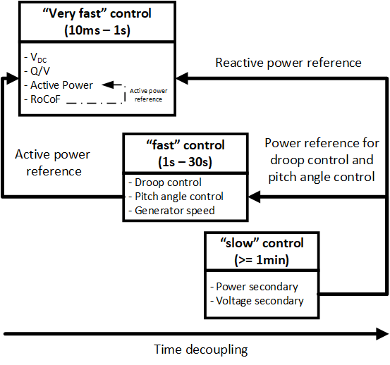
Figure 1: Time decoupling structure for grid connected PPMs

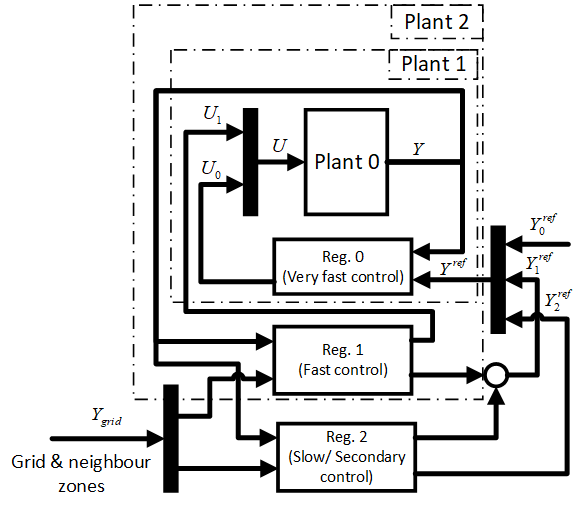
Figure 2: Time and space separation of the control of the grid connected PPMs

3.3 A new concept for the control model

Separation of the V and f dynamics mentioned in Section 2 led till now to 2 different models in power systems community: for V regulation, the Single Machine Infinite Bus (SMIB) model given in Fig 3 and for f regulation, the one in Fig. 4 (e.g., [20], [31]). As explained before, this hypothesis of separation of dynamics is no longer valid in power systems with high RES penetration. Indeed, in case of power converters, V and f dynamics are mixed and both fast. As a consequence, V and f controls should be synthesized together, i.e., in coordination. Advanced methods of control need a control model, i.e., a low dimensional model of the plant to be controlled. This is extracted from the full model of the plant and should preserve the dynamics of interest. The model we propose here is given in Fig. 5. It consists of the full model of the PPM to be controlled, an equivalent AC line of reactance $X_{\infty}$ and a Grid Dynamic Equivalent (bloc GDE) which provides the grid frequency. The line $X_{\infty}$ plays the same role as in classic SMIB model in Fig. 3. This accounts for the grid short-circuit power at PPM connection bus A and it is computed in a standard way (see, e.g., [32]). The difference with the SMIB is that electrical frequency of bus B is not fixed at the nominal grid frequency (50 or 60Hz), but given by GDE by the following swing equation

$$2H\frac{d\omega_{f}}{dt}=P_{G}-P_{L}-D_{u}\Delta\omega_{f}$$ (1)

and the three-phase voltage dynamics

$$\begin{array}[]{l}\begin{aligned} {V_{B}}^{a}=Vsin(\theta_{f})\\ {V_{B}}^{b}=Vsin(\theta_{f}-2\frac{\pi}{3})\\ {V_{B}}^{c}=Vsin(\theta_{f}+2\frac{\pi}{3}).\end{aligned}\end{array}$$ (2)

H is the equivalent inertia of the rest of the system (in which the controlled PPM is inserted), $P_{G}$ is the global active power produced in the rest of the system and $P_{L}$ corresponds to the global load of the system. $P_{m}$ is a constant input for the PPM control problem. Dynamics (1) is stabilized by the damping factor $D_{u}$ and a simple integrator for deviation of $\omega_{f}$ from the nominal grid frequency if a secondary frequency control is considered. H is computed by classic equivalencing methods (e.g., [20]) used in frequency studies. The difference between GDE and model in Fig. 4 is that GDE captures also voltage dynamics in compliance with the f ones.

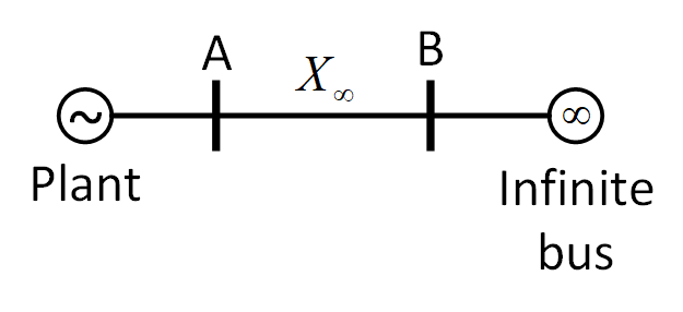
Figure 3: Voltage control model: SMIB

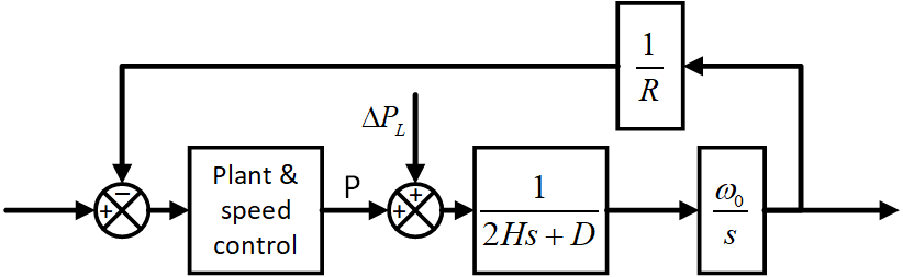
Figure 4: Frequency control model

Figure 5: New control model for single PPM

Figure 6: New control model for multiple PPMs

Notice also that a common practice is to use a large classic synchronous generator as equivalent for the rest of the system. Indeed, one can thus chose its inertia constant H close to the inertia of the rest of the system. However, this kind of equivalent is not suitable for at least 2 reasons: first, as the model of a physical synchrounous generator is used, one should also add voltage and frequency regulations for this machine. The latter ones have no significance in the model and their parameters would influence the resulting dynamics. Next, the order of such a model (the dimension of its state) is much higher than the one of the proposed GDE (which is 1).

If several PPMs have to be controlled, the structure of the control model is one of the 2 equivalent ones given in Fig. 6.

4 Application to wind PPMs

Control strategy presented in the above section will be here developed for 2 wind PPMs based on Permanent Magnet Synchronous Generators (PMSGs).

4.1 Synthesis of the control model

The control model of the first layer of regulation (i.e., Plant 0 in Fig. 2) is thus the one in Fig. 6 with n=2 and the PPM of Fig. 8, i.e., the one in Fig. 7.

Figure 7: Two PMSGs connected to the grid

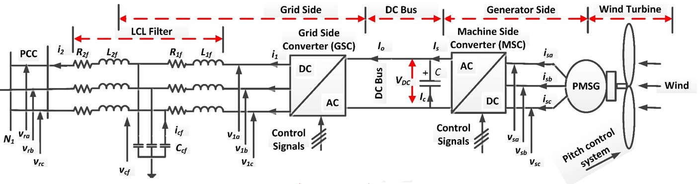
Figure 8: Wind PMSG based PPM

Using the nonlinear model in [33] for the 2 PMSGs, one obtains

$${\tiny\left\{\begin{array}[]{l}\begin{aligned} \frac{{d{i_{11d}}}}{{dt}}=&-{\omega_{fb}}\frac{{{R_{11f}}{i_{11d}}}}{{{L_{11f}}}}+{\omega_{fb}}{\omega_{f}}{i_{11q}}-{\omega_{fb}}\frac{{{v_{cf1d}}}}{{{L_{11f}}}}+\frac{1}{2}{\omega_{fb}}\frac{{{\beta_{11d}}{v_{DC1}}}}{{{L_{11f}}}}\end{aligned}\\ \begin{aligned} \frac{{d{i_{11q}}}}{{dt}}=&-{\omega_{fb}}\frac{{{R_{11f}}{i_{11q}}}}{{{L_{11f}}}}-{\omega_{fb}}{\omega_{f}}{i_{11d}}-{\omega_{fb}}\frac{{{v_{cf1q}}}}{{{L_{11f}}}}+\frac{1}{2}{\omega_{fb}}\frac{{{\beta_{11q}}{v_{DC1}}}}{{{L_{11f}}}}\end{aligned}\\ \begin{aligned} &\frac{{d{i_{21d}}}}{{dt}}=-{\omega_{fb}}\frac{{{R_{21f}}{i_{21d}}}}{{{L_{21f}}}}+{\omega_{fb}}{\omega_{f}}{i_{21q}}+{\omega_{fb}}\frac{{{v_{cf1d}}}}{{{L_{21f}}}}\\ &-{\omega_{fb}}\frac{1}{{{L_{21f}}}}\frac{1}{{{n_{1}}}}\left({{a_{r1d}}{i_{21d}}+{b_{r1d}}{i_{21q}}+{c_{r1d}}{i_{22d}}+{d_{r1d}}{i_{22q}}+{e_{r1d}}V}\right)\end{aligned}\\ \begin{aligned} &\frac{{d{i_{21q}}}}{{dt}}=-{\omega_{fb}}\frac{{{R_{21f}}{i_{21q}}}}{{{L_{21f}}}}-{\omega_{fb}}{\omega_{f}}{i_{21d}}+{\omega_{fb}}\frac{{{v_{cf1q}}}}{{{L_{21f}}}}\\ &-{\omega_{fb}}\frac{1}{{{L_{21f}}}}\frac{1}{{{n_{1}}}}\left({{a_{r1q}}{i_{21d}}+{b_{r1q}}{i_{21q}}+{c_{r1q}}{i_{22d}}+{d_{r1q}}{i_{22q}}+{e_{r1q}}V}\right)\end{aligned}\\ \begin{aligned} \frac{{d{v_{cf1d}}}}{{dt}}=&{\omega_{fb}}\frac{{{i_{11d}}}}{{{C_{f1}}}}-{\omega_{fb}}\frac{{{i_{21d}}}}{{{C_{f1}}}}+{\omega_{fb}}{\omega_{f}}{v_{cf1q}}\end{aligned}\\ \begin{aligned} \frac{{d{v_{cf1q}}}}{{dt}}=&{\omega_{fb}}\frac{{{i_{11q}}}}{{{C_{f1}}}}-{\omega_{fb}}\frac{{{i_{21q}}}}{{{C_{f1}}}}-{\omega_{fb}}{\omega_{f}}{v_{cf1d}}\end{aligned}\\ \begin{aligned} \frac{{d{i_{s1d}}}}{{dt}}=&-{\omega_{fb}}\frac{{{R_{s1}}{i_{s1d}}}}{{{L_{s1}}}}+{\Omega_{b}}{p_{1}}{\Omega_{1}}{i_{s1q}}-\frac{1}{2}{\omega_{fb}}\frac{{{\beta_{s1d}}{v_{DC1}}}}{{{L_{s1}}}}\end{aligned}\\ \begin{aligned} \frac{{d{i_{s1q}}}}{{dt}}=&-{\omega_{fb}}\frac{{{R_{s1}}{i_{s1q}}}}{{{L_{s1}}}}-{\Omega_{b}}{p_{1}}{\Omega_{1}}{i_{s1d}}+{\Omega_{b}}\frac{{{p_{1}}{\Psi_{f1}}{\Omega_{1}}}}{{{L_{s1}}}}-\frac{1}{2}{\omega_{fb}}\frac{{{\beta_{s1q}}{v_{DC1}}}}{{{L_{s1}}}}\end{aligned}\\ \begin{aligned} \frac{{d{v_{DC1}}}}{{dt}}=&-{\omega_{fb}}\frac{3}{{4{C_{1}}}}{\beta_{11d}}{i_{11d}}-{\omega_{fb}}\frac{3}{{4{C_{1}}}}{\beta_{11q}}{i_{11q}}+{\omega_{fb}}\frac{3}{{4{C_{1}}}}{\beta_{s1d}}{i_{s1d}}\\ &+{\omega_{fb}}\frac{3}{{4{C_{1}}}}{\beta_{s1q}}{i_{s1q}}\end{aligned}\\ \begin{aligned} \frac{{d{\Omega_{1}}}}{{dt}}=&\frac{1}{{2{H_{1}}}}\frac{{{P_{m1}}}}{{{\Omega_{1}}}}-\frac{1}{{2{H_{1}}}}\frac{{{\Omega_{b}}}}{{{\omega_{fb}}}}\frac{3}{2}{p_{1}}{\Psi_{f1}}{i_{s1q}}-\frac{1}{{2{H_{1}}}}{D_{L1}}{\Omega_{1}}\end{aligned}\end{array}\right.}$$ (3)

$${\tiny\left\{\begin{array}[]{l}\begin{aligned} \frac{{d{i_{12d}}}}{{dt}}=&-{\omega_{fb}}\frac{{{R_{12f}}{i_{11d}}}}{{{L_{12f}}}}+{\omega_{fb}}{\omega_{f}}{i_{12q}}-{\omega_{fb}}\frac{{{v_{cf2d}}}}{{{L_{12f}}}}+\frac{1}{2}{\omega_{fb}}\frac{{{\beta_{12d}}{v_{DC2}}}}{{{L_{12f}}}}\end{aligned}\\ \begin{aligned} \frac{{d{i_{12q}}}}{{dt}}=&-{\omega_{fb}}\frac{{{R_{12f}}{i_{11q}}}}{{{L_{12f}}}}-{\omega_{fb}}{\omega_{f}}{i_{12d}}-{\omega_{fb}}\frac{{{v_{cf2q}}}}{{{L_{12f}}}}+\frac{1}{2}{\omega_{fb}}\frac{{{\beta_{12q}}{v_{DC2}}}}{{{L_{12f}}}}\end{aligned}\\ \begin{aligned} &\frac{{d{i_{22d}}}}{{dt}}=-{\omega_{fb}}\frac{{{R_{22f}}{i_{22d}}}}{{{L_{22f}}}}+{\omega_{fb}}{\omega_{f}}{i_{22q}}+{\omega_{fb}}\frac{{{v_{cf2d}}}}{{{L_{22f}}}}\\ &-{\omega_{fb}}\frac{1}{{{L_{22f}}}}\frac{1}{{{n_{2}}}}\left({{a_{r2d}}{i_{21d}}+{b_{r2d}}{i_{21q}}+{c_{r2d}}{i_{22d}}+{d_{r2d}}{i_{22q}}+{e_{r2d}}V}\right)\end{aligned}\\ \begin{aligned} &\frac{{d{i_{22q}}}}{{dt}}=-{\omega_{fb}}\frac{{{R_{22f}}{i_{22q}}}}{{{L_{22f}}}}-{\omega_{fb}}{\omega_{f}}{i_{22d}}+{\omega_{fb}}\frac{{{v_{cf2q}}}}{{{L_{22f}}}}\\ &-{\omega_{fb}}\frac{1}{{{L_{22f}}}}\frac{1}{{{n_{2}}}}\left({{a_{r2q}}{i_{21d}}+{b_{r2q}}{i_{21q}}+{c_{r2q}}{i_{22d}}+{d_{r2q}}{i_{22q}}+{e_{r2q}}V}\right)\end{aligned}\\ \begin{aligned} \frac{{d{v_{cf2d}}}}{{dt}}=&{\omega_{fb}}\frac{{{i_{12d}}}}{{{C_{f2}}}}-{\omega_{fb}}\frac{{{i_{22d}}}}{{{C_{f2}}}}+{\omega_{fb}}{\omega_{f}}{v_{cf2q}}\end{aligned}\\ \begin{aligned} \frac{{d{v_{cf2q}}}}{{dt}}=&{\omega_{fb}}\frac{{{i_{12q}}}}{{{C_{f2}}}}-{\omega_{fb}}\frac{{{i_{22q}}}}{{{C_{f2}}}}-{\omega_{fb}}{\omega_{f}}{v_{cf2d}}\\ \frac{{d{i_{s2d}}}}{{dt}}=&-{\omega_{fb}}\frac{{{R_{s2}}{i_{s2d}}}}{{{L_{s2}}}}+{\Omega_{b}}{p_{2}}{\Omega_{2}}{i_{s2q}}-\frac{1}{2}{\omega_{fb}}\frac{{{\beta_{s2d}}{v_{DC2}}}}{{{L_{s2}}}}\end{aligned}\\ \begin{aligned} \frac{{d{i_{s2q}}}}{{dt}}=&-{\omega_{fb}}\frac{{{R_{s2}}{i_{s2q}}}}{{{L_{s2}}}}-{\Omega_{b}}{p_{2}}{\Omega_{2}}{i_{s2d}}+{\Omega_{b}}\frac{{{p_{2}}{\Psi_{f2}}{\Omega_{2}}}}{{{L_{s2}}}}-\frac{1}{2}{\omega_{fb}}\frac{{{\beta_{s2q}}{v_{DC2}}}}{{{L_{s2}}}}\end{aligned}\\ \begin{aligned} \frac{{d{v_{DC2}}}}{{dt}}=&-{\omega_{fb}}\frac{3}{{4{C_{2}}}}{\beta_{12d}}{i_{12d}}-{\omega_{fb}}\frac{3}{{4{C_{2}}}}{\beta_{12q}}{i_{12q}}+{\omega_{fb}}\frac{3}{{4{C_{2}}}}{\beta_{s2d}}{i_{s2d}}\\ &+{\omega_{fb}}\frac{3}{{4{C_{2}}}}{\beta_{s2q}}{i_{s2q}}\end{aligned}\\ \begin{aligned} \frac{{d{\Omega_{2}}}}{{dt}}=&\frac{1}{{2{H_{2}}}}\frac{{{P_{m2}}}}{{{\Omega_{2}}}}-\frac{1}{{2{H_{2}}}}\frac{{{\Omega_{b}}}}{{{\omega_{fb}}}}\frac{3}{2}{p_{2}}{\Psi_{f2}}{i_{s2q}}-\frac{1}{{2{H_{2}}}}{D_{L2}}{\Omega_{2}};{D_{L2}}=\frac{{\Omega_{b}^{2}{f_{2}}}}{{{S_{b}}}}\end{aligned}\end{array}\right.}$$ (4)

For the rest of the above presented control model, one should consider (1) with ${D_{u}}=\frac{{\omega_{b}^{2}D}}{{{S_{b}}}}$, $P_{G}=P_{m}+P_{e}$, where $P_{m}$ is the generated power in the rest of the system and

$${\small{P_{e}}={a_{Pe}}{i_{21d}}+{b_{Pe}}{i_{21q}}+{c_{Pe}}{i_{22d}}+{d_{Pe}}{i_{22q}}}$$ (5)

is the power generated by the two PMSGs.

The dynamics of pitch angle of the two PMSGs are totally decoupled from the rest of the PMSGs dynamics [34] - [35]:

$$\left\{\begin{array}[]{l}\frac{{d{\beta_{PMSG1}}}}{{dt}}=-\frac{1}{{{\tau_{C1}}}}{\beta_{PMSG1}}+\frac{1}{{{\tau_{C1}}}}{\beta_{PMSG1ref}}\\ \frac{{d{\beta_{PMSG2}}}}{{dt}}=-\frac{1}{{{\tau_{C2}}}}{\beta_{PMSG2}}+\frac{1}{{{\tau_{C2}}}}{\beta_{PMSG2ref}}\end{array}\right.$$ (6)

where

$$\left\{\begin{array}[]{l}{\beta_{\min}}\leq{\beta_{PMSG1}},{\beta_{PMSG2}}\leq{\beta_{\max}}\\ {\left({\frac{{d\beta}}{{dt}}}\right)_{\min}}\leq\frac{{d{\beta_{PMSG1}}}}{{dt}},\frac{{d{\beta_{PMSG2}}}}{{dt}}\leq{\left({\frac{{d\beta}}{{dt}}}\right)_{\max}}\end{array}\right.$$

Typically, as in [34] - [35], these limitations come from the servo motor:

$$\left\{\begin{array}[]{l}{\tau_{C1}}=0.2\left(s\right);{\tau_{C2}}=0.2\left(s\right)\\ {\beta_{\min}}=0\left({\deg}\right);{\beta_{\max}}=20\left({\deg}\right)\\ {\left({\frac{{d\beta}}{{dt}}}\right)_{\min}}=-10\left({\deg}\right);{\left({\frac{{d\beta}}{{dt}}}\right)_{\max}}=10\left({\deg}\right)\end{array}\right.$$

The pitch angle will then be controlled separately from the dynamics of the two PMSGs.

The active power will be calculated at the generator rather than at the converter to avoid the mismatch in generating generator speed reference based on MPPT and deloaded control

$$\left\{\begin{gathered}{P_{1}}=\frac{3}{2}\frac{{{\Omega_{b}}}}{{{\omega_{fb}}}}p{\psi_{f1}}{i_{s1q}}{\Omega_{1}}\hfill\\ {P_{2}}=\frac{3}{2}\frac{{{\Omega_{b}}}}{{{\omega_{fb}}}}p{\psi_{f2}}{i_{s2q}}{\Omega_{2}}.\hfill\\ \end{gathered}\right.$$ (7)

The reactive power will be calculated from the voltages of capacitor in the LCL filter rather than directly from the converters to avoid direct relationship between input and output of the system

$$\left\{\begin{gathered}{Q_{1}}={i_{11d}}{v_{cf1q}}-{i_{11q}}{v_{cf1d}}\hfill\\ {Q_{2}}={i_{12d}}{v_{cf2q}}-{i_{12q}}{v_{cf2d}}.\hfill\\ \end{gathered}\right.$$ (8)

4.2 Global structure of the proposed control

According to the time-separation strategy presented in Section 3, to satisfy the control specifications listed in Sections 2 and 3, the structure given in Fig. 9 is proposed for the control of 2 wind PPMs. At this stage, droop control and control for RoCoF improvement were inherited from the classic approach presented in Appendices 8.1 and 8.2. They are placed in fast and, respectively, very fast parts of the global scheme. As they are not model-based controls, a state-space model will be constructed (in the next section) only for Plant 0.

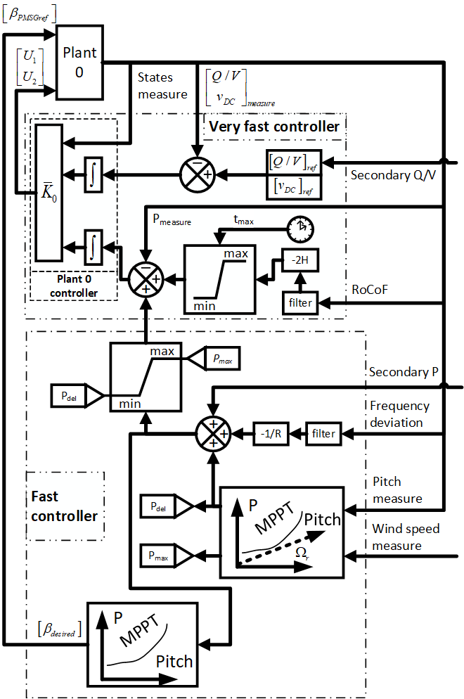
Figure 9: Global control for PMSG with local services and frequency support

4.3 Augmented system for plant 0 controller

For the very fast loop control, consider the mixed sensibility control structure as in Fig. 10.

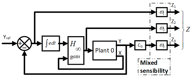
Figure 10: Very fast loop control

Based on (3), (4), (5), (6), (7) and (8), the system can be formed in the state-space form with disturbance

$$\left\{{\begin{array}[]{*{20}{l}}{{{\dot{X}}_{e0}}=A{X_{e0}}+{B_{1}}U+{B_{2}}W}\\ {{Y_{e0}}=C{X_{e0}}}\end{array}}\right.$$ (9)

The state, input, output and disturbance of the system are

$$\begin{gathered}{X_{1}}=\left[{{i_{11d}},{i_{11q}},{i_{21d}},{i_{21q}},{v_{cf1d}},{v_{cf1q}},{i_{s1d}},{i_{s1q}},{v_{DC1}},{\Omega_{1}}}\right]\hfill\\ {X_{2}}=\left[{{i_{12d}},{i_{12q}},{i_{22d}},{i_{22q}},{v_{cf2d}},{v_{cf2q}},{i_{s2d}},{i_{s2q}},{v_{DC2}},{\Omega_{2}}}\right]\hfill\\ {X_{e0}}={\left[{\begin{array}[]{*{20}{c}}{{X_{1}}}&{{X_{2}}}&{{\omega_{f}}}\end{array}}\right]^{T}};W={\left[{\begin{array}[]{*{20}{c}}{{P_{m1}}}&{{P_{m2}}}&{{P_{L}}}\end{array}}\right]^{T}}\hfill\\ {U_{1}}=\left[{{\beta_{11d}},{\beta_{11q}},{\beta_{21d}},{\beta_{21q}}}\right];{U_{2}}=\left[{{\beta_{12d}},{\beta_{12q}},{\beta_{22d}},{\beta_{22q}}}\right]\hfill\\ U=\left[{\begin{array}[]{*{20}{c}}{{U_{1}}}&{{U_{2}}}\end{array}}\right]\hfill\\ {Y_{e0}}={\left[{\begin{array}[]{*{20}{l}}{{Q_{1}}}&{{P_{1}}}&{{v_{DC1}}}&{{Q_{2}}}&{{P_{2}}}&{{v_{DC2}}}\end{array}}\right]^{T}}\hfill\\ \end{gathered}$$

The error between output and the reference is

$${e_{e0}}=-C{X_{e0}}+{Y_{e0ref}}$$ (10)

where the entries of $Y_{e0ref}$ are the reactive power references, the active power references and the DC voltage references.

Weight $\omega_{3}$ will improve high-frequencies roll-off in order to cancel the oscillatory effect of LCL filters in Fig. 8. Indeed, it is well-known that these filters provide poor damped oscillatory modes at high frequency, around 500Hz in the case of our system. As this frequency is much higher than the one related to the very fast part of our control, roll-off improvement via loop-shaping will be sufficient. Modal analysis (not presented here because of the lack of the space) showed that these modes are observable in the Q measures. $C_{Q}=\left[{\begin{array}[]{*{20}{c}}1&0&0&0&0&0\\ 0&0&0&1&0&0\end{array}}\right]$ was chosen to target reactive power at the output of this bloc. The structure of the filter $\omega_{3}$ is standard (see, e.g., [30]). Let

$$\left\{\begin{gathered}{{\dot{X}}_{{\omega_{3}}}}={A_{{\omega_{3}}}}{X_{{\omega_{3}}}}+{B_{{\omega_{3}}}}{C_{Q}}CX\hfill\\ {Y_{{\omega_{3}}}}={C_{{\omega_{3}}}}{X_{{\omega_{3}}}}+{D_{{\omega_{3}}}}{C_{Q}}CX\hfill\\ \end{gathered}\right.$$ (11)

be its state representation.

The weight $\omega_{1}$ is usually used to improve reference tracking and disturbance rejection. However, in our case, the integral action structure in Fig. 10 is perfectly fit for zero-error reference-tracking based on internal model principle. Also, to comply with $H_{\infty}$ optimization to minimize the norm from disturbance to output error, which is the best way for disturbance rejection, $\omega_{1}$ is chosen as unit gain: $\omega_{1}=1$.

As in our situation there is no particular need for limiting control effort in a particular frequency band, to simplify the control structure, $\omega_{2}$ will be ignored: $\omega_{2}=0$.

The extended state for the purpose of step reference tracking are

$${{\bar{X}}_{e0}}={\left[{\begin{array}[]{*{20}{c}}{{X_{e0}}}&{{X_{{\omega_{3}}}}}&{Int\_e}\end{array}}\right]^{T}};Int\_e=\int{{e_{e0}}dt}$$ (12)

The resulting extended system is

$$\left\{\begin{gathered}{{{\dot{\bar{X}}}_{e0}}}={{\bar{A}}_{e0}}{{\bar{X}}_{e0}}+{{\bar{B}}_{1e0}}U+{{\bar{B}}_{2e0}}{\bar{W}}_{e0}\hfill\\ \overline{Y}={\overline{C}_{e0}}{{\bar{X}}_{e0}}+{\overline{D}_{1e0}}U\hfill\\ \end{gathered}\right.$$ (13)

where

$$\begin{gathered}{{\bar{W}}_{e0}}={\left[{\begin{array}[]{*{20}{c}}{{W^{T}}}&{{Y_{e0ref}}}\end{array}}\right]^{T}};{{\bar{D}}_{1e0}}=\left[{\begin{array}[]{*{20}{c}}0&I\\ 0&0\end{array}}\right];\hfill\\ {{\bar{A}}_{e0}}=\left[{\begin{array}[]{*{20}{c}}A&0&0\\ {{B_{{\omega_{3}}}}{C_{Q}}C}&{{A_{{\omega_{3}}}}}&0\\ {-C}&0&0\end{array}}\right];{{\bar{B}}_{1e0}}=\left[{\begin{array}[]{*{20}{c}}{{B_{1}}}\\ 0\\ 0\end{array}}\right];\hfill\\ {{\bar{B}}_{2e0}}=\left[{\begin{array}[]{*{20}{c}}{{B_{1}}}&0\\ 0&0\\ 0&I\end{array}}\right];{C_{e0}}=\left[{\begin{array}[]{*{20}{c}}{-C}&0&0\\ {{D_{{\omega_{3}}}}{C_{Q}}C}&{{C_{{\omega_{3}}}}}&0\end{array}}\right]\hfill\\ \end{gathered}$$

5 Proposed H-infinity Controller

The controller synthesis for very fast control loop is given in what follows.

Consider the extended linear system (13) of very fast control loop with the state feedback control

$$U={\bar{K}}_{0}{\bar{X}}_{e0}.$$ (14)

5.1 Controller synthesis

The influence of the disturbance ${\bar{W}}_{e0}$ to the output $\bar{Y}$ is

$$\bar{Y}\left(s\right)=G\left(s\right){\bar{W}}_{e0}\left(s\right),$$ (15)

where

$${\small G\left(s\right)=({{\bar{C}}_{e0}}+{{\bar{D}}_{1e0}}{{\bar{K}}_{0}}){\left({sI-\left({{{\bar{A}}_{e0}}+{{\bar{B}}_{1e0}}{{\bar{K}}_{0}}}\right)}\right)^{-1}}{{\bar{B}}_{2e0}}}$$ (16)

It is obvious that [34], [36] - [39]

$${\left\|{\bar{Y}}\right\|_{2}}\leq{\left\|G\right\|_{\infty}}{\left\|{{{\bar{W}}_{e0}}}\right\|_{2}}$$ (17)

Problem 1

For the linear system (13) and (15), the H-infinity problem is to design a stabilizing static state feedback control law (14) such that

$${\left\|G\right\|_{\infty}}<\gamma$$ (18)

for a minimum positive scalar $\gamma$.

5.2 Derivation of stability and robustness conditions

The main result for the global asymptotic stability of a globally H-infinity controller are summarized by the following theorem.

Theorem 1

The H-infinity problem has a solution if and only if there exist a matrix $W_{P}$ and a symmetric positive definite matrix $X_{P}$ , through the LMI-based minimization such that

$$\mathop{minimize}\limits_{{X_{P}},{W_{P}}}\;\;\gamma$$

subject to

$$\left[{\begin{array}[]{*{20}{c}}\Psi&{{{\bar{B}}_{2e0}}}&{{{\left({{{\bar{C}}_{e0}}{X_{P}}+{{\bar{D}}_{1e0}}{W_{P}}}\right)}^{T}}}\\ {\bar{B}_{2e0}^{T}}&{-\gamma I}&0\\ {{{\bar{C}}_{e0}}{X_{P}}+{{\bar{D}}_{1e0}}{W_{P}}}&0&{-\gamma I}\end{array}}\right]<0$$

where

$$\Psi={\left({{{\bar{A}}_{e0}}{X_{P}}+{{\bar{B}}_{1e0}}{W_{P}}}\right)^{T}}+{{\bar{A}}_{e0}}{X_{P}}+{{\bar{B}}_{1e0}}{W_{P}}$$ (19)

In this case, the solution of the problem is

$${{\bar{K}}_{0}}={W_{P}}X_{P}^{-1}$$ (20)

Proof 1

It is well-known [36] - [39] that for a linear system given by

$$\left\{\begin{array}[]{l}\dot{X}=AX+BU\\ Y=CX+DU\end{array}\right.$$ (21)

or by

$$\left\{\begin{array}[]{l}Y=G\left(s\right)U\\ G\left(s\right)=C{\left({sI-A}\right)^{-1}}B+D\end{array}\right.$$ (22)

a solution to the H-infinity problem can be found if and only if there exist a symmetric positive definite matrix $X_{p}$ , such that

$$\left[{\begin{array}[]{*{20}{c}}{{X_{P}}{A^{T}}+A{X_{P}}}&B&{{X_{P}}{C^{T}}}\\ {{B^{T}}}&{-\gamma I}&{{D^{T}}}\\ {C{X_{P}}}&D&{-\gamma I}\end{array}}\right]<0$$ (23)

Written for the linear system with disturbance (equation (13)), where $G\left(s\right)$ is in the form of equation (16), the latter condition yields

$$\left\{\begin{array}[]{l}{\small\left[{\begin{array}[]{*{20}{c}}\Psi&{{{\bar{B}}_{2e0}}}&{{X_{P}}{{\left({{{\bar{C}}_{e0}}+{{\bar{D}}_{1e0}}{{\bar{K}}_{0}}}\right)}^{T}}}\\ {\bar{B}_{2e0}^{T}}&{-\gamma I}&0\\ {\left({{{\bar{C}}_{e0}}+{{\bar{D}}_{1e0}}{{\bar{K}}_{0}}}\right){X_{P}}}&0&{-\gamma I}\end{array}}\right]<0}\\ \Psi={X_{P}}{\left({{{\bar{A}}_{e0}}+{{\bar{B}}_{1e0}}{{\bar{K}}_{0}}}\right)^{T}}+\left({{{\bar{A}}_{e0}}+{{\bar{B}}_{1e0}}{{\bar{K}}_{0}}}\right){X_{P}}\end{array}\right.$$ (24)

This is equivalent to

$$\left\{\begin{array}[]{l}{\scriptsize\left[{\begin{array}[]{*{20}{c}}\Psi&{{{\bar{B}}_{2e0}}}&{{{\left({{{\bar{C}}_{e0}}{X_{P}}+{{\bar{D}}_{1e0}}{{\bar{K}}_{0}}{X_{P}}}\right)}^{T}}}\\ {\bar{B}_{2e0}^{T}}&{-\gamma I}&0\\ {{{\bar{C}}_{e0}}{X_{P}}+{{\bar{D}}_{1e0}}{{\bar{K}}_{0}}{X_{P}}}&0&{-\gamma I}\end{array}}\right]<0}\\ {\footnotesize\Psi={\left({{{\bar{A}}_{e0}}{X_{P}}+{{\bar{B}}_{1e0}}{{\bar{K}}_{0}}{X_{P}}}\right)^{T}}+\left({{{\bar{A}}_{e0}}{X_{P}}+{{\bar{B}}_{1e0}}{{\bar{K}}_{0}}{X_{P}}}\right)}\end{array}\right.$$ (25)

and, by defining ${W_{P}}={{\bar{K}}_{0}}{X_{P}}$, the inequality turns into the one of Theorem 1.

5.3 Implementation of the controller

The state-feedback of the above extended system results into a multivariable PI controller

$$U={{\bar{K}}_{0}}{{\bar{X}}_{e0}}={{\bar{K}}_{0}}\left[{\begin{array}[]{*{20}{c}}{{X_{e0}}}\\ {{X_{{\omega_{3}}}}}\\ {\int{{e_{e0}}dt}}\end{array}}\right]$$ (26)

This is the control structure of Plant 0 controller in Fig. 9.

6 Simulations and results

For the system in Fig. 7, simulations are carried out with a full model (detailed models from the standard Matlab libraries for all elements of the systems (generators, lines, converters, loads, …)) developped in SimPower Toolbox of Matlab. The PMSGs are identical and of 8MW nominal power. The load of the whole power system is $P_{L}=55000MW$. A limited but visible support is thus expected from PMSGs to grid frequency. The initial operating point for all test scenarios is at generated power $P_{e}=0.6527pu$ for each PMSG.

To check the PMSGs’ control specifications and objectives listed in Sections 2 and 3, several scenarios have been constructed:

• Scenario 1 - Local services: to test active power, reactive power and DC voltage control, steps are applied on control reference variables.

• Scenario 2 - Voltage services (Q/V): to test voltage services, a three-phase metallic short-circuit is performed in the middle of the AC line $X_{1}$ in Fig. 7. The short-circuit starts at t = 100s and it is cleared at t = 100.11s.

• Scenario 3 - Frequency services: to test frequency services, the grid load is step increased by 10Mw at t = 100s and restored at t = 800s.

• Scenario 4 - Comparison between the proposed coordinated control and classic vector control: for that purpose, the classic vector control presented in Appendix 8.3 have been implemented and used. The same short-circuit as in Scenario 2 was considered.

6.1 Scenario 1: Local services

Fig. 11 gives the reactive power response of PMSG1 to steps on $Q_{1_{ref}}$ in both directions (negative and, next, positive). One can notice nominal response times (around 4s for 5$\%$ step tracking) and non oscillatory transient dynamics. Fig. 12 contains same kind of nominal responses to similar steps on $P_{1_{ref}}$. In Fig. 13 it is shown the response of the DC voltage control to a change of reference $V_{DC_{1_{ref}}}$ from 2.5pu to 2.625pu. The time response is around 5s and the transient is smooth. The behavior of the second PMSG for local services is similar (Figs. 14, 15, 16).

6.2 Scenario 2: Voltage services (Q/V)

Short-circuit responses of PMSG1 are given in Figs. 17, 18 and 19. They show a good fault ride through capability, both for voltage and reactive power dynamics. The duration of the transient at the beginning and at the end of short-circuit event is very short, around 4ms and, after, the terminal voltage is stabilized at its desired value. Also, thanks to coordinated control, the impact of the speed of the generator is minimal. Indeed, the generator speed (Fig. 19) only experiences a very small deviation in a short time and without any overshoot/undershoot after the clearing of the short-circuit.

Notice also that, due to the location of the short-circuit (on line $X_{1}$), its impact on PMSG1 is stronger than on PMSG2. Indeed, one can see in Fig. 18 that the terminal voltage of PMSG1 drops almost to zero. For PMSG2, the effect of short-circuit is insignificant as seen in Fig. 20 to Fig. 22. In Fig. 20, the reactive power is slightly deviated, around 4$\%$ of its nominal value during the event, and only oscillates around 4ms before coming back to its operating point. In Fig. 21, the terminal voltage of PMSG2 is maintained at its nominal value, with only a short transient of about 10ms at the beginning and at the end of the event. Moreover, these transients come with a relatively low deviation peak, at only around 4$\%$. In Fig. 22, the influence of short-circuit on generator speed is infinitesimal, with only a very small deviation for a very short duration.

6.3 Scenario 3: Frequency services

Figs. 24 and 27 show very fast increase of the active powers of both PMSGs in response to the simulated load variation of the system given in Fig. 23: they are increased immediately, from deloaded point (0.65pu) to nearly maximum value (0.8pu). This proves effectiveness of the very fast control loop controller (through inertia control) of Fig. 9. Indeed, without inertia control, no variation is registered (black curves in the same figures). This frequency support helps to diminish the severe drop of RoCoF as observed in Fig. 30. The generator speeds, given in Fig. 25 and Fig. 28, decrease and come close to their optimal values (blue curves/w1_optimal), which help to maintain the produced power. However, this immediate increase in power can only be maintained during a short laps of time (a couple seconds). After that, the active power of each PMSG tends to come back close to nominal value to ensure machines’ stability.

After a couple of seconds, the fast loop of the proposed control (Fig. 9) is activated, through MPPT and droop control, to request more power in order to reduce grid frequency deviation (Fig. 31). Both generators use their deloding reserves (10$\%$) to increase their powers from deloaded points (0.65pu) to their maximum values of MPPT (0.8pu) as seen in Fig. 24 and, respectively, Fig. 27. As a result, generator speeds and pitch angles come close to optimal values as can be seen in Fig. 28, Fig. 25 and, respectively, Fig. 29, Fig. 26 (optimal value for pitch angle is 0 deg). At t = 800s, as the grid load comes back to its nominal value, the active powers for both PMSGs are brought to their nominal values by the very fast and fast controllers of each machine (Fig. 9). This is the same for grid frequency, generator speeds and pitch angles, as observed in Figs. 31, 28, 25, 29, 26.

6.4 Scenario 4: Comparison between proposed coordinated control and classic vector control

One can see in Fig. 32 and Fig. 34 that the proposed control provides a better dynamics for $V_{DC}$ than classic vector control. Indeed, transient is less oscillating, which results in shorter response time (around 5 times). This is also the case for the terminal voltage where more sustained oscillations are registered with the vector control (Fig. 33).

Same behavior is noticed for PMSG2 (Fig. 35 and 34), even though the short-circuit less impacts this machine (as explained in Section 6.2).

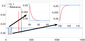
Figure 11: The reactive power (pu) of PMSG1 (local services)

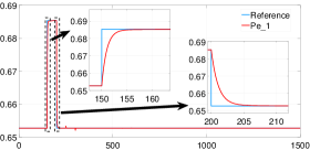
Figure 12: The active power (pu) of PMSG1 (local services)

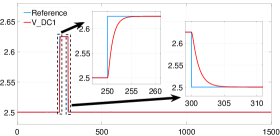
Figure 13: The DC voltage (pu) of PMSG1 (local services)

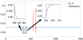
Figure 14: The reactive power (pu) of PMSG2 (local services)

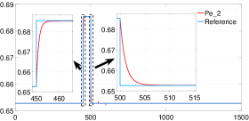
Figure 15: The active power (pu) of PMSG2 (local services)

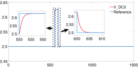
Figure 16: The DC voltage (pu) of PMSG2 (local services)

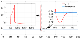
Figure 17: The reactive power (pu) of PMSG1 (Voltage service)

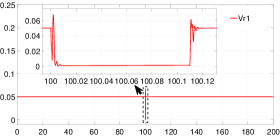
Figure 18: The AC terminal voltage $V_{r1}$ (pu) of PMSG1 (Voltage service)

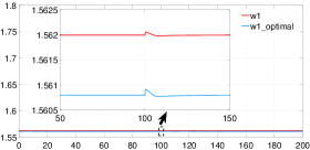
Figure 19: The generator speed (pu) of PMSG1 (Voltage service)

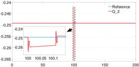
Figure 20: The reactive power (pu) of PMSG2 (Voltage service)

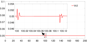
Figure 21: The AC terminal voltage $V_{r2}$ (pu) of PMSG2 (Voltage service)

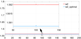
Figure 22: The generator speed (pu) of PMSG2 (Voltage service)

Figure 23: The grid load changing scenario (frequency service)

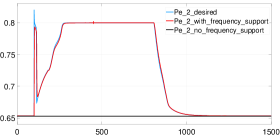
Figure 24: Active power (pu) of PMSG2 (frequency service)

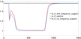
Figure 25: Generator speed of PMSG2 (frequency service)

Figure 26: Pitch angle (deg) of PMSG2 (frequency service)

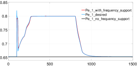
Figure 27: Active power (pu) of PMSG1 (frequency service)

Figure 28: Generator speed of PMSG1 (frequency service)

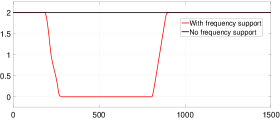
Figure 29: Pitch angle (deg) of PMSG1 (frequency service)

Figure 30: RoCoF (pu) behavior (frequency service)

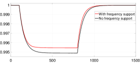
Figure 31: Frequency (pu) of the grid (frequency service)

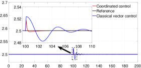
Figure 32: DC voltage (pu) of PMSG1 (coordinated control vs vector control)

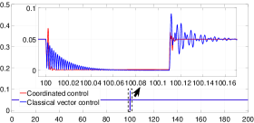
Figure 33: AC terminal voltage $V_{r1}$ (pu) of PMSG1 (coordinated control vs vector control)

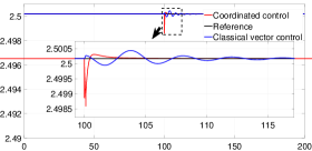
Figure 34: DC voltage (pu) of PMSG2 (coordinated control vs vector control)

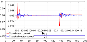
Figure 35: AC terminal voltage $V_{r2}$ (pu) of PMSG2 (coordinated control vs vector control)

7 Conclusions

To address full participation of PPMs in grid ancillary services, we have first critically reviewed the classic regulation framework and main differences at dynamic level between PPMs and classic synchronous generators. It has been concluded that old hypothesis of separation between V and f dynamics should be skipped at all levels: modeling and synthesis of controls. Coordination should be achieved at these levels as well as for other aspects. As a consequence, a new control model which gathers all dynamics of interest has been proposed. Based on it, a strategy of robust advanced model-based control was proposed. The proposed approach is based on the overall time-scales separation of the dynamics of the global system and of its control objectives. This makes a significant difference with the classic vector control and related approaches which propose several simple PI loops around each actuator of the global system. Maximum coordination is achieved as all actuators and dynamics of interest are taken into account in the control model on which the synthesis of the control is based. This coordination is among the 2 converters of a same PPM or even among converters (and other dynamics) of several PPMs when control is addressed for a class of PPMs as in the example treated.

This aspect will be fully developped in following work and publications in the framework of H2020 POSYTYF project where a class of PPMs will be controlled in a new concept called Dynamic Virtual Power Plant to maximize RES participation to grid ancillary services.

The proposed control methodology and concepts are general and can be used for any type of PPM or RES connected to the grid with power converters. Elements of the time-decoupling diagram in Fig. 1 should be specifically used for each case. For example, in case of a storage element (battery), it is expected to control only the very fast dynamics.

Synthesis of the control in close relation to the time-scale of phenomena and objectives paves the way to participation of PPMs and RESs to grid ancillary services. This means to really integrate the new sources into today existing secondary V and f controls, at the same level of exigences as the classic synchronous generators and not only to provide some implicit grid support, which is difficult to quantify and relay on it. Integration of PPMs into the secondary level control, i.e., stage ”‘slow”’ in Fig. 2 is also a next step in our work in POSYTYF project.

The presented methodology is a model-based one which is open to any advanced control. Here loop-shaping was achieved by H-infinity synthesis. In next work we will add fuzzyfication to improve behavior with respect to nonlinearities and variations of system operating conditions. Also, extended validation in hardware-in-the loop environment will be next done.

8 Classic control of wind PPMs

8.1 Droop control with deloading methods

Droop control, since the era of classical synchronous generators, is an important control loop to regulate frequency based on active power control of a grid [20]. However, with RES, especially wind generators, to minimize the overall cost, the main goal was to maximize power generation using MPPT [3]-[19], [4], and this leaves no room for active power regulation in case of grid incident. Hence, a new method emerged, which try to reserve an amount of energy by regulating the produced energy at lower level than MPPT, called deloading control [4], [18], [40]-[43].

10% is a typical value for the reserve of the deloading control using generator speed control. Higher reserve can be ensured if pitch angle control is used in addition.

Firstly, consider the pitch angle is kept at 0 (deg), the deloading relationship between wind speed, generator speed and wind turbine mechanical power is given in Fig. 36.

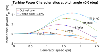
Figure 36: The output power at different wind speeds at MPPT and at 10% deload

To understand the deloading strategy, consider the wind turbine is operating at wind speed of 16m/s. The wind turbine will produce power at 10$\%$ deloading point A of Fig. 37 to reserve 10$\%$ of its power capacity.

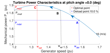
Figure 37: The generator speed deloading strategy at wind speed of 16 m/s

To utilize this reserved power for frequency support, a droop relationship is established [20]

$$\Delta{P_{ref}}=-\frac{1}{R}\Delta f,$$ (27)

where $\Delta{P_{ref}}$ is the required amount of change in power when there is a change in frequency $\Delta f$.

A consequence of a shortage in power of the the grid is a fall in grid frequency [20]. This fall will partly be compensated by the reserved power of wind turbine. At this moment, through the droop relationship (27), the wind turbine will have to move its operating point from A to B to increase its mechanical power. The operating point is now at

$$P_{mref}=P_{mdel}+\Delta{P_{ref}}=P_{mdel}-\frac{1}{R}\Delta f.$$ (28)

This $P_{mref}$ will be used to determine desired generator speed $\Omega_{ref}$, and through generator speed control to shift the operating point of wind turbine. This action can easily be achieved by a look-up table [4] [40] - [43], but with a cost in delay due to the time for searching the equivalent value of $\Omega_{ref}$. To overcome this, because the two points of optimal and deloading points are very close, it is possible to consider that the three points A, B and C are collinear. As a consequence, the relationship between $P_{mref}$ and $\Omega_{ref}$ is [4]

$${P_{mref}}={P_{mdel}}+\left({{P_{mopt}}-{P_{mdel}}}\right)\frac{{{\Omega_{del}}-{\Omega_{ref}}}}{{{\Omega_{del}}-{\Omega_{opt}}}}$$ (29)

Based on (29), the value of $\Omega_{ref}$ is

$${\Omega_{ref}}={\Omega_{del}}-\left({{\Omega_{del}}-{\Omega_{opt}}}\right)\left({-\frac{1}{R}\frac{{\Delta f}}{{{P_{mopt}}-{P_{mdel}}}}}\right)$$ (30)

Secondly, consider all the deloading relationships between wind speed, generator speed, pitch angle and wind turbine mechanical power in the 3D scheme of Fig. 38.

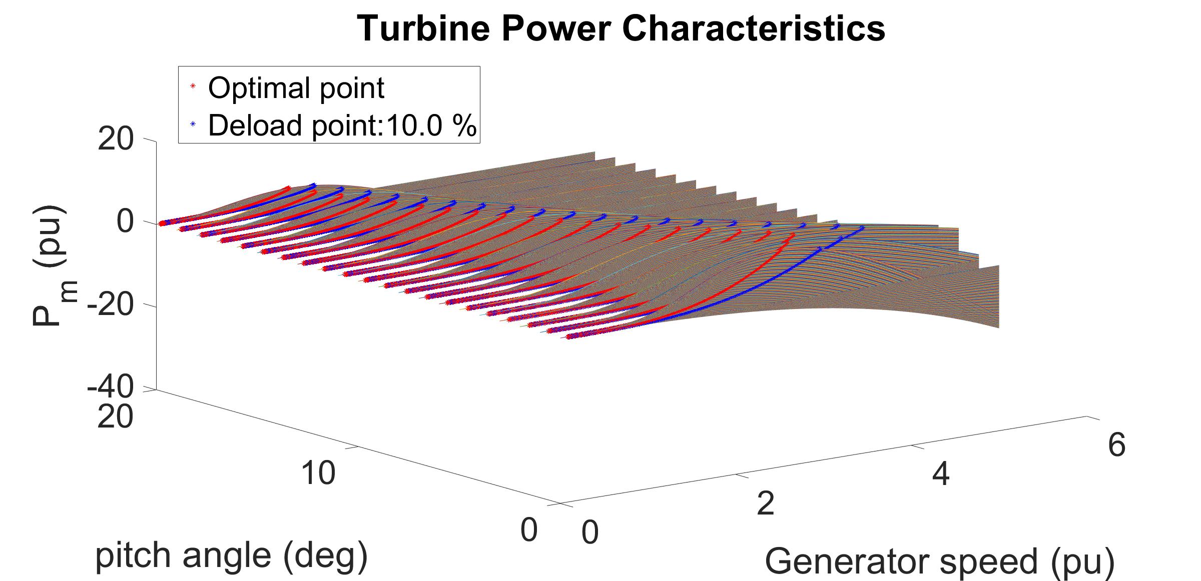
Figure 38: The output power at different wind speeds (1-30 m/s) at MPPT and at 10% deload

Again, to deload the wind turbine using pitch angle control, the pitch angle will be kept at deloading point instead of optimal point (0 deg) [4], [40] - [43]. To understand the deloading pitch angle strategy, consider the wind turbine is operating at constant wind speed 12 (m/s) for Fig. 39.

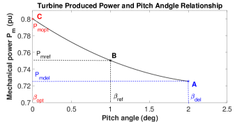
Figure 39: The pitch angle deloading strategy at wind speed of 12 m/s

At steady-state, wind turbine will operate at point A with pitch angle $\beta_{del}$ and produce power at $P_{del}$. Following a request to increase the power (28) via the droop control (27), the pitch angle will be changed from point A to point B.

Once again, a look-up table can be used, but this results in introducing significant delay into the control loop. This problem can be dealt with the same method as in (29). The relationship between desired produced power $P_{mref}$ and desired pitch angle $\beta_{ref}$ is then

$${P_{mref}}={P_{mdel}}+\left({{P_{mopt}}-{P_{mdel}}}\right)\frac{{{\beta_{del}}-{\beta_{ref}}}}{{{\beta_{del}}-{\beta_{opt}}}}$$ (31)

From droop control relationship (28) and (31), the desired pitch angle $\beta_{ref}$ is

$${\beta_{ref}}={\beta_{del}}-\left({{\beta_{del}}-{\beta_{opt}}}\right)\left({-\frac{1}{R}\frac{{\Delta f}}{{{P_{mopt}}-{P_{mdel}}}}}\right).$$ (32)

8.2 Inertia control for wind turbine

Currently, there are two popular types of fast support for RoCoF improvement for RES: hidden inertia control [4] [7]-[11] and fast power reserve [4], [12]-[15]. Because of the lack of the space, only the first one is presented and used (Fig. 40).

Hidden inertia [8], or virtual inertia [7], or inertia emulation [4] is basically a way to react to the change of RoCoF, by feedback RoCoF to the reference of electrical torque or electrical active power

$$\Delta{P_{eref}}=K\frac{{df}}{{dt}},$$ (33)

where $\Delta{P_{eref}}$ is the ”needed” power to compensate the drop in RoCoF, $f$ is the nearby grid frequency and $K$ is the inertia response loop gain, which depends on inertia constant of wind turbine and may depend on frequency $f$ as in [4] - [8]. The hidden inertia control can also be modified and utilized at the same time with droop control to achieve better frequency support [4]-[7].

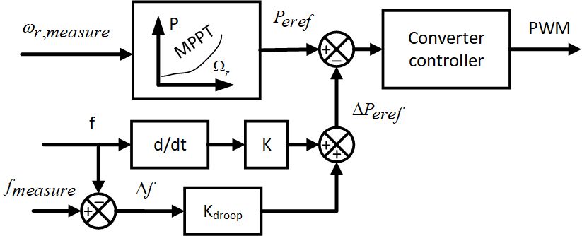
Figure 40: The hidden inertia control structure [4]

The gain $K$ is estimated starting from the change of power of the grid due to frequency variation

$$\Delta{P_{L}}=2H\frac{{df}}{{dt}},$$ (34)

where $H$ is the inertia constant of the grid, $f$ is grid frequency and $\Delta{P_{L}}$ is the total power change. The idea behind inertia control is to immediately produce the same amount of total power to keep the RoCoF as small as possible. This means that the required produced power should be

$$\Delta{P_{eref}}=-\Delta{P_{L}}=-2H\frac{{df}}{{dt}}$$ (35)

Hence, the gain $K$ and droop gain are

$$\left\{\begin{array}[]{l}K=-2H\\ {K_{droop}}=-\frac{1}{R}\end{array}\right.$$ (36)

8.3 Vector control for converters

Vector control is a very popular method in the field of power converters control [23], [24] - [27]. It is structured in two control loops decoupled in time by the control itself: one fast for the current, called inner loop and one slower for the voltage (and/or reactive and active power), called outer loop. They are given in Fig. 41 for the grid-side converter.

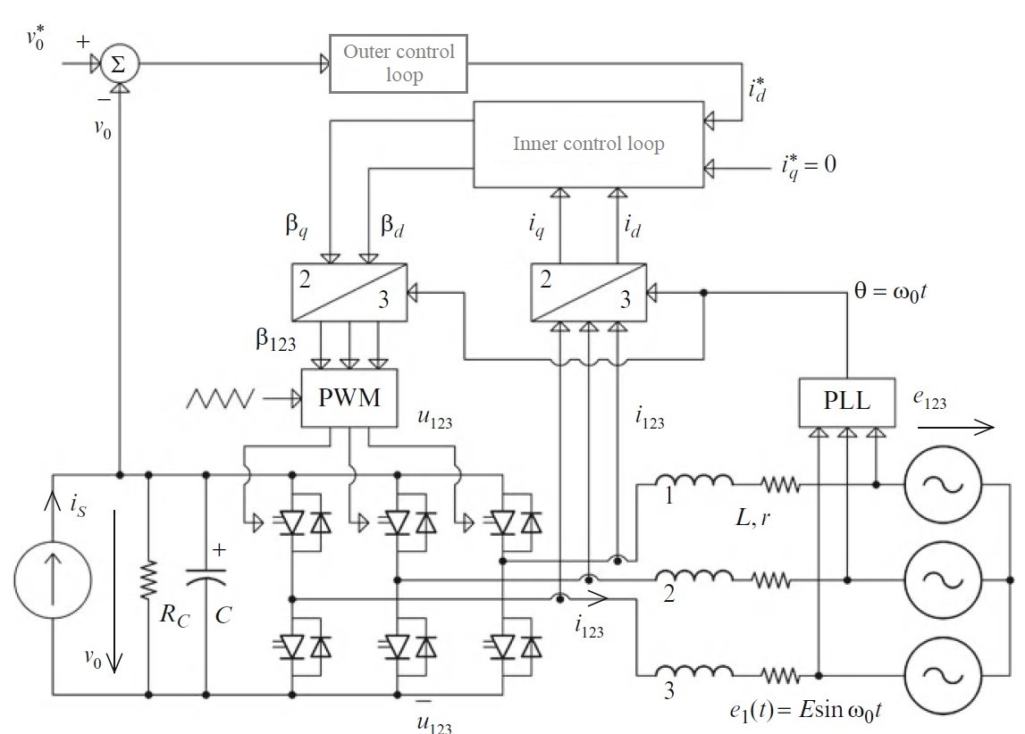
Figure 41: The vector control structure for grid-side converter [27]

In the inner loop detailed in Fig. 42, the currents in each d and q axis are controlled by a PI controller. Two cross connections among these controls are included to diminish interaction. The PI controllers parameters $K_{pC}$ and $T_{iC}$ are chosen by forcing the damping ratio and the time constant of the current closed-loop into desired values [26] [27]. The references $i^{\star}_{d}$ and $i^{\star}_{q}$ are filtered to compensate for the zeros induced in the closed-loop [26], [27].

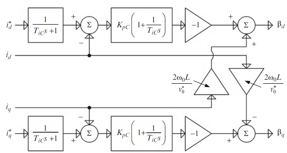
Figure 42: The vector control inner loop of current control [27]

The outer loop of voltage control, is actually a loop to produce the desired value of $i_{d}$, which is the reference for the inner loop in Fig. 41. As for the inner loop, the PI controllers parameters are chosen by forcing the damping ratio and the time constant of the voltage closed-loop into desired values [26], [27]. The time constant of this outer loop should be around 10-100 times higher that the one of the inner loop to allow independent design of the controller.

References

• [1] Gils, H. C., Scholz, Y., Pregger, T., de Tena, D. L., $\&$ Heide, D. (2017). Integrated modelling of variable renewable energy-based power supply in Europe. Energy, 123, 173-188.
• [2] ”Renewables 2021 global status report.”, https://www.ren21.net/wp-content/uploads/2019/05/GSR2021$\_$Full$\_$Report.pdf.
• [3] FernΓ‘ndez-GuillamΓ³n, A., GΓ³mez-LΓ‘zaro, E., Muljadi, E., $\&$ Molina-GarcΓ­a, Á. (2019). Power systems with high renewable energy sources: A review of inertia and frequency control strategies over time. Renewable and Sustainable Energy Reviews, 115, 109369.
• [4] Dreidy, M., Mokhlis, H., $\&$ Mekhilef, S. (2017). Inertia response and frequency control techniques for renewable energy sources: A review. Renewable and sustainable energy reviews, 69, 144-155.
• [5] Rietveld, G., Wright, P. S., $\&$ Roscoe, A. J. (2020). Reliable rate-of-change-of-frequency measurements: Use cases and test conditions. IEEE Transactions on Instrumentation and Measurement, 69(9), 6657-6666.
• [6] ENTSO-E (16. Dec. 2020), Inertia and Rate of Change of Frequency (RoCoF).
• [7] Zhang, Z., Wang, Y., Li, H., $\&$ Su, X. (2013, June). Comparison of inertia control methods for DFIG-based wind turbines. In 2013 IEEE ECCE Asia Downunder (pp. 960-964). IEEE.
• [8] Zhang, Z. S., Sun, Y. Z., Lin, J., $\&$ Li, G. J. (2012). Coordinated frequency regulation by doubly fed induction generator-based wind power plants. IET Renewable Power Generation, 6(1), 38-47.
• [9] Margaris, I. D., Papathanassiou, S. A., Hatziargyriou, N. D., Hansen, A. D., $\&$ Sorensen, P. (2012). Frequency control in autonomous power systems with high wind power penetration. IEEE Transactions on sustainable energy, 3(2), 189-199.
• [10] You, R., Barahona, B., Chai, J., $\&$ Cutululis, N. A. (2015). Frequency support capability of variable speed wind turbine based on electromagnetic coupler. Renewable Energy, 74, 681-688.
• [11] Su, C., $\&$ Chen, Z. (2012, July). Influence of wind plant ancillary frequency control on system small signal stability. In 2012 IEEE Power and Energy Society General Meeting (pp. 1-8). IEEE.
• [12] El Itani, S., Annakkage, U. D., $\&$ Joos, G. (2011, July). Short-term frequency support utilizing inertial response of DFIG wind turbines. In 2011 IEEE Power and Energy Society General Meeting (pp. 1-8). IEEE.
• [13] Keung, P. K., Li, P., Banakar, H., $\&$ Ooi, B. T. (2008). Kinetic energy of wind-turbine generators for system frequency support. IEEE Transactions on Power Systems, 24(1), 279-287.
• [14] FernΓ‘ndez-GuillamΓ³n, A., Vigueras-RodrΓ­guez, A., GΓ³mez-LΓ‘zaro, E., $\&$ Molina-GarcΓ­a, Á. (2018). Fast power reserve emulation strategy for VSWT supporting frequency control in multi-area power systems. Energies, 11(10), 2775.
• [15] FernΓ‘ndez-GuillamΓ³n, A., Villena-Lapaz, J., Vigueras-RodrΓ­guez, A., GarcΓ­a-SΓ‘nchez, T., $\&$ Molina-GarcΓ­a, Á. (2018). An adaptive frequency strategy for variable speed wind turbines: Application to high wind integration into power systems. Energies, 11(6), 1436.
• [16] Requirements for generators, ENTSOE, https://www.entsoe.eu/network$\_$codes/rfg/.
• [17] Hwang, M., Muljadi, E., Park, J. W., SΓΈrensen, P., $\&$ Kang, Y. C. (2016). Dynamic droop–based inertial control of a doubly-fed induction generator. IEEE Transactions on Sustainable Energy, 7(3), 924-933.
• [18] Chang-Chien, L. R., Lin, W. T., $\&$ Yin, Y. C. (2010). Enhancing frequency response control by DFIGs in the high wind penetrated power systems. IEEE transactions on power systems, 26(2), 710-718.
• [19] Hohm, D. P., $\&$ Ropp, M. E. (2003). Comparative study of maximum power point tracking algorithms. Progress in photovoltaics: Research and Applications, 11(1), 47-62.
• [20] Kundur, P. (1994), Power Systems Stability and Control, EPRI.
• [21] Pattabiraman, D., Lasseter, R. H., $\&$ Jahns, T. M. (2018, August). Comparison of grid following and grid forming control for a high inverter penetration power system. In 2018 IEEE Power $\&$ Energy Society General Meeting (PESGM) (pp. 1-5). IEEE.
• [22] Rodriguez, P., $\&$ Lai, N. B. (2021). Grid-following and grid-forming PV and wind turbines. In Control of Power Electronic Converters and Systems (pp. 499-521). Academic Press.
• [23] Irwin, J. D. (2002). Control in power electronics: selected problems. Elsevier.
• [24] Kazmierkowski, M. P., $\&$ Malesani, L. (1998). Current control techniques for three-phase voltage-source PWM converters: A survey. IEEE Transactions on industrial electronics, 45(5), 691-703.
• [25] Choi, J. W., $\&$ Sul, S. K. (1998). Fast current controller in three-phase AC/DC boost converter using dq axis crosscoupling. IEEE Transactions on Power Electronics, 13(1), 179-185.
• [26] Bajracharya, C., Molinas, M., Suul, J. A., $\&$ Undeland, T. M. (2008). Understanding of tuning techniques of converter controllers for VSC-HVDC. In Nordic Workshop on Power and Industrial Electronics (NORPIE/2008), June 9-11, 2008, Espoo, Finland. Helsinki University of Technology.
• [27] Bacha, S., Munteanu, I., $\&$ Bratcu, A. I. (2014). Power electronic converters modeling and control. Advanced textbooks in control and signal processing, 454, 454.
• [28] PΓΆschke, F., $\&$ Schulte, H. (2020, July). Model-based Nonlinear Filter Design for Tower Load Reduction of Wind Power Plants with Active Power Control Capability. In 2020 IEEE International Conference on Fuzzy Systems (FUZZ-IEEE) (pp. 1-6). IEEE.
• [29] Bratcu, A. I., Munteanu, I., Bacha, S., Picault, D., $\&$ Raison, B. (2010). Cascaded dc–dc converter photovoltaic systems: Power optimization issues. IEEE Transactions on Industrial Electronics, 58(2), 403-411.
• [30] Skogestad, S., $\&$ Postlethwaite, I. (2007). Multivariable feedback control: analysis and design (Vol. 2). New York: Wiley.
• [31] Bevrani, H. (2014). Robust power system frequency control. Springer.
• [32] Xiong, X., Ouyang, J., $\&$ Jin, J. (2011, October). Calculation of steady-state short-circuit current of wind turbines with doubly fed induction generator. In 2011 International Conference on Advanced Power System Automation and Protection (Vol. 3, pp. 1782-1788). IEEE.
• [33] Kamal, E., $\&$ Marinescu, B. (2019, September). Converter Nonlinear Fuzzy Control of PMSG-Based for Wind Energy System in Network Context. In 2019 IEEE PES Innovative Smart Grid Technologies Europe (ISGT-Europe) (pp. 1-5). IEEE.
• [34] Van, T. L., Nguyen, T. H., $\&$ Lee, D. C. (2015). Advanced pitch angle control based on fuzzy logic for variable-speed wind turbine systems. IEEE Transactions on Energy Conversion, 30(2), 578-587.
• [35] Yin, X. X., Lin, Y. G., Li, W., Gu, Y. J., Wang, X. J., $\&$ Lei, P. F. (2015). Design, modeling and implementation of a novel pitch angle control system for wind turbine. Renewable Energy, 81, 599-608.
• [36] Ngo, H. T., Kamal, E., Marinescu, B., $\&$ Xavier, F. (2020, November). Robust $H_{\infty}$ Decentralized Control Design for HVDC Link Embedded in a Large-scale AC Grid. In 2020 Electrical Power and Energy Conference.
• [37] Duan, G. R., $\&$ Yu, H. H. (2013). LMIs in control systems: analysis, design and applications. CRC press.
• [38] Boyd, S., El Ghaoui, L., Feron, E., $\&$ Balakrishnan, V. (1994). Linear matrix inequalities in system and control theory. Society for industrial and applied mathematics.
• [39] Zhang, F. (Ed.). (2006). The Schur complement and its applications (Vol. 4). Springer Science $\&$ Business Media.
• [40] Luo, H., Hu, Z., Zhang, H., $\&$ Chen, H. (2018). Coordinated active power control strategy for deloaded wind turbines to improve regulation performance in AGC. IEEE Transactions on Power Systems, 34(1), 98-108.
• [41] Zhang, X., Chen, Y., Wang, Y., Zha, X., Yue, S., Cheng, X., $\&$ Gao, L. (2019). Deloading power coordinated distribution method for frequency regulation by wind farms considering wind speed differences. IEEE Access, 7, 122573-122582.
• [42] Baros, S., $\&$ IliΔ‡, M. D. (2017). Distributed torque control of deloaded wind DFIGs for wind farm power output regulation. IEEE Transactions on Power Systems, 32(6), 4590-4599.
• [43] Dong, Z., Li, Z., Dong, Y., Jiang, S., $\&$ Ding, Z. (2020). Fully-distributed deloading operation of DFIG-based wind farm for load sharing. IEEE Transactions on Sustainable Energy, 12(1), 430-440.