Asymptotic densities of planar Lévy walks: a non-isotropic case

Abstract

Lévy walks are a particular type of continuous-time random walks which results in a super-diffusive spreading of an initially localized packet. The original one-dimensional model has a simple schematization that is based on starting a new unidirectional motion event either in the positive or in the negative direction. We consider two-dimensional generalization of Lévy walks in the form of the so-called XY-model. It describes a particle moving with a constant velocity along one of the four basic directions and randomly switching between them when starting a new motion event. We address the ballistic regime and derive solutions for the asymptotic density profiles. The solutions have a form of first-order integrals which can be evaluated numerically. For specific values of parameters we derive an exact expression. The analytic results are in perfect agreement with the results of finite-time numerical samplings.

I Introduction

The idea of Lévy walks (LWs) yosi1 ; yosi2 can be sketched as follows: A particle moves, straightforwardly and with the constant velocity $v_{0}$, for some time $\tau_{i}$, then stops, changes, instantaneously and randomly, the direction of its motion, and starts to move along the newly chosen direction. The particle is launched from the origin at the initial instant of time and the process is iterated until the time reaches the set threshold $t$, $\sum_{i=1}^{N}\tau_{i}+\bar{\tau}_{N+1}=t$, $0<\bar{\tau}_{N+1}<\tau_{N+1}$ (that is, the last motion event is stopped once the time threshold is reached). The duration of a motion event is drawn from a probability density function (pdf) with a slowly decaying power-law tail, $\psi(\tau)\propto\tau^{-1-\gamma}$, $0<\gamma<2$. During the last two decades, this simple – at first glance – model has found applications in different fields, ranging from physics and chemistry to biology and sociology, as an instrument to describe and understand complex transport phenomena rmp .

Most of the existing theoretical results were derived for one dimensional LW models rmp . Although the 1$d$ set-up allows for a lot of flexibility in tailoring of a particular experiment-relevant model, the geometry of the resulting process is simple: the particle moves either to the right or to the left at any instant of time. Generalization of this scheme to 2$d$ is not straightforward and several models have been proposed  yosi2 ; prl2016 , with two of them being most intuitive.

In the uniform model prl2016 , the direction of the next flight is determined by choosing, randomly and uniformly, a point on a unit circle (on the surface of the unit sphere $\mathcal{S}^{d}$ in the $d$-dimensional case yosi2 ; marcin2016 ; marcin2017 ; fouxon2017 ). The resulting process is spatially isotropic and this allows to reduce the set of spatial variables to a single one, $r=|\textbf{r}|$.

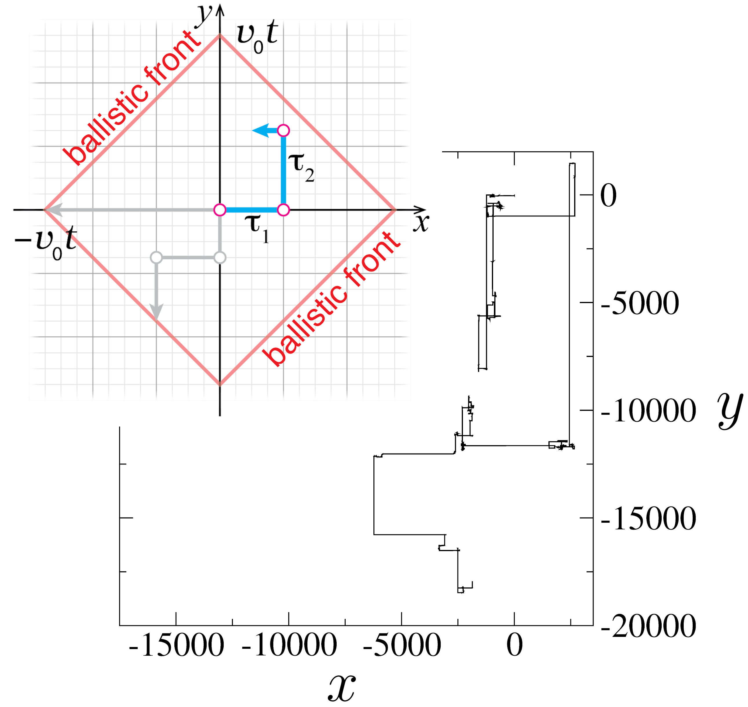
Figure 1: XY-model of planar Lévy walks. A particle is allowed to move, with a speed $v_{0}$, only along one Cartesian axis at a time, which is chosen randomly at the re-orientation points $\circ$. The ballistic front is determined by the square $|x|+|y|=v_{0}t$. Geometry of the process imparts the shape of the corresponding trajectory which exhibits a distinctive rectangular web-like pattern with long ballistic re-locations along the two axes. The parameters here are $\gamma=1/2$, $\upsilon_{0}=1$ and $\tau_{0}=1$.

In the XY-model yosi3 ; prl2016 , the motion of the particle is restricted to four basic Cartesian directions; see Fig. 1. When initiating a new motion event, one has to roll a four-sided die dice , draw duration $\tau_{i}$, and then set the particle into a ballistic motion along the corresponding direction. The resulting process is essentially non-isotropic and that is imprinted in the shape of pdf $P(\textbf{r},t)$ specifying the probability of finding the particle at a vicinity of point r at time $t$ prl2016 ; fouxon2017 . The XY-model is not just an abstract mathematical construction. For example, it reproduces Hamiltonian kinetics in egg-crate potentials yosi3 and in infinite horizon billiards zarfaty1 . Depending on the symmetry of a potential or size of the scatterers in a billiard, the motion can be restricted to four, eight, or larger even number of basic directions  cristadoro . The XY-model can be generalized to reproduce kinetics of these systems zarfaty2 .

In the ballistic regime, $0<\gamma<1$, mean flight time $\langle\tau\rangle=\int_{0}^{\infty}\tau\psi(\tau)\,d\tau$ diverges and the mean squared displacement (MSD) of the corresponding LW processes exhibit universal ballistic scaling, $\langle r^{2}(t)\rangle=\int_{0}^{t}r^{2}P(\textbf{r},t)\,d\tau\propto t^{2}$. A method to compute asymptotic pdf’s for one-dimensional ballistic Lévy walks was presented in Ref. bal1 . Consequently, asymptotic pdf’s of the uniform model were evaluated in Ref. marcin2016 .

Here we advance further along this line and address ballistic regime of the XY-model. Evidently, the corresponding spatially non-isotropic spreading is more complex than the one obtained with the uniform model. Remarkably, as we demonstrate, even in this case it is possible to compute the asymptotic densities and derive analytical expressions.

II Model and basic equations

Following the basic idea of LWs yosi2 ; rmp , we consider a particle which moves with constant velocity $v_{0}$ and performs instantaneous re-orientations at random instants of time. The time between two consequent re-orientation events is a random variable distributed according to pdf

$$\psi(\tau)=\frac{1}{\tau_{0}}\frac{\gamma}{(1+\tau/\tau_{0})^{1+\gamma}},\quad 0<\gamma<1,$$ (1)

where $\tau_{0}>0$. The re-orientation process is determined by pdf $h(\mathbf{v})$ which specifies the direction of vector $\mathbf{v}$, $|\mathbf{v}|=v_{0}$.

The particle starts from the origin at the initial instant of time. The probability to have the particle moving without re-orientation up to time $t$ is $\Psi(t)=\int_{t}^{\infty}\mathrm{d}\tau\psi(\tau)$. Pdf $P(\mathbf{r},t)$, after being transformed into the Fourier-Laplace domain, obeys the equation

$$P(\mathbf{k},s)=\frac{\int\mathrm{d}\mathbf{v}\,\Psi(s+i\mathbf{k}\cdot\mathbf{v})h(\mathbf{v})}{1-\int\mathrm{d}\mathbf{v}\,\psi(s+i\mathbf{k}\cdot\mathbf{v})h(\mathbf{v})},$$ (2)

where $\mathbf{k}=\{k_{x},k_{y}\}$ and $s$ are coordinates in the two-dimensional Fourier and one-dimensional Laplace spaces, respectively.

In the case of the XY-model, we have re-orientation pdf $h(\mathbf{v})=[\delta(|v_{x}|-v_{0})\delta(v_{y})+\delta(v_{x})\delta(|v_{y}|-v_{0})]/4$. The ballistic front has the form of a square defined by the equation $|x|+|y|=v_{0}t$; see Fig. 1. In this case equation (2) can be rewritten as

$$P(\mathbf{k},s)=\frac{\sum_{\kappa\in K}\Psi(s+i\kappa v_{0})}{\sum_{\kappa\in K}[1-\psi(s+i\kappa v_{0})]},$$ (3)

where $K=\{\pm k_{x},\pm k_{y}\}$. The structure of the equation highlights the fact that $P(\mathbf{r},t)$ is an even (symmetric) function with respect to the space coordinates and is also invariant under permutation $x\leftrightarrow y$. Henceforth we assume that $v_{0}=1$ and consistently re-normalized time which now is measure in units of space. It would be enough to replace $t\mapsto v_{0}t$ in the final expressions in order to obtain the answer for arbitrary $v_{0}$.

In the long-time limit, the waiting-time distribution (1), can be approximated in the Laplace domain as

$$\psi(s)\simeq 1-\tau_{0}^{\gamma}\Gamma(1-\gamma)s^{\gamma}+o(s^{\gamma}).$$ (4)

In the limit $\mathbf{k},s\rightarrow 0$ (which corresponds to both $\mathbf{r}$ and $t$ are going to infinity), we obtain from Eqs. (3-4) the following expression:

$$P_{XY}(\mathbf{k},s)=\frac{\sum_{\kappa\in K}(s+i\kappa)^{\gamma-1}}{\sum_{\kappa\in K}(s+i\kappa)^{\gamma}}.$$ (5)

It is noteworthy that, by using the notion of fractional material derivatives  MBSB2002(r) ; SM2003 ; MetzlerKlafter2004 , a deterministic equation governing the evolution of the pdf in the original space, can be derived.

III Derivation of asymptotic pdf $\mathcal{P}(\overline{x},\overline{y})$

We start with recasting Eq. (5) into

$$P_{XY}(\mathbf{k},s)=Q(k_{x},k_{y},s)+Q(k_{y},k_{x},s),$$ (6)

where

$$Q(k_{x},k_{y},s)=\frac{(s+ik_{x})^{\gamma-1}+(s-ik_{x})^{\gamma-1}}{\sum_{\kappa\in K}(s+i\kappa)^{\gamma}}.$$ (7)

It is enough therefore to find the inverse of function $Q(k_{x},k_{y},s)$ [the inverse of $Q(k_{y},k_{x},s)$ could be obtained by permuting $x\leftrightarrow y$].

We introduce the following two functions:

$$g_{1}\!\left(\frac{ik_{x}}{s},u\right)=\left[\left(1+\frac{ik_{x}}{s}\right)^{\gamma-1}+\left(1-\frac{ik_{x}}{s}\right)^{\gamma-1}\right]\exp\!\left\{-u\!\left[\left(1+\frac{ik_{x}}{s}\right)^{\gamma}+\left(1-\frac{ik_{x}}{s}\right)^{\gamma}\right]\right\},$$ (8)

$$g_{2}\!\left(\frac{ik_{y}}{s},u\right)=\exp\!\left\{-u\!\left[\left(1+\frac{ik_{y}}{s}\right)^{\gamma}+\left(1-\frac{ik_{y}}{s}\right)^{\gamma}\right]\right\}.$$ (9)

By implementing identity

$$1/\varrho=\int_{0}^{\infty}\mathrm{d}u\,e^{-u\varrho}\,\,(\mathrm{Re}\,\varrho>0),$$ (10)

we can recast Eq. (7) as

$$Q(k_{x},k_{y},s)=\frac{1}{s}\int_{0}^{\infty}\mathrm{d}u~{}g_{1}\!\left(\frac{ik_{x}}{s},u\right)g_{2}\!\left(\frac{ik_{y}}{s},u\right).~{}~{}$$ (11)

By using properties of the Laplace transform for a derivative and a convolution (which we denote with $\circ$), from Eq. (11) we obtain

$$Q(x,y,t)=\frac{\partial}{\partial t}\int_{0}^{\infty}\mathrm{d}u\,G_{1}(x,t,u)\circ G_{2}(y,t,u),$$ (12)

where

$$G_{1}(x,t,u) =\mathcal{F}^{-1}_{x}\mathcal{L}^{-1}\!\left\{\frac{1}{s}g_{1}\!\left(\frac{ik_{x}}{s},u\right)\right\},$$ (13)

$$G_{2}(y,t,u) =\mathcal{F}^{-1}_{y}\mathcal{L}^{-1}\!\left\{\frac{1}{s}g_{2}\!\left(\frac{ik_{y}}{s},u\right)\right\}.$$ (14)

Thus we obtained the expression for $Q(x,y,t)$ which demands not a three-step inverse transform, $\mathcal{F}^{-1}_{x}\mathcal{F}^{-1}_{y}\mathcal{L}^{-1}$, but a pair of two-step inverse transforms, $\mathcal{F}^{-1}_{x}\mathcal{L}^{-1}$ and $\mathcal{F}^{-1}_{y}\mathcal{L}^{-1}$, of functions $\frac{1}{s}g_{1}\!\left(\frac{ik_{x}}{s}\right)$ and $\frac{1}{s}g_{2}\!\left(\frac{ik_{y}}{s}\right)$, respectively. To find the inverses, we follow a procedure similar to that given in Ref. GL2001 (see Appendix A) and obtain

$$G_{1}(x,t,u) =-\frac{1}{2\pi i\,x}\!\lim\limits_{\,\epsilon\rightarrow 0^{+}}\!\!\left[g_{1}\!\left(-\frac{1}{x/t+i\epsilon},u\right)\right.$$

$$\mathrel{\phantom{=}}\left.-g_{1}^{*}\!\left(-\frac{1}{x/t+i\epsilon},u\right)\right]$$ (15)

and

$$G_{2}(y,t,u) =-\frac{1}{2\pi i\,y}\!\lim\limits_{\,\epsilon\rightarrow 0^{+}}\!\!\left[g_{2}\!\left(-\frac{1}{y/t+i\epsilon},u\right)\right.$$

$$\mathrel{\phantom{=}}\left.-g_{2}^{*}\!\left(-\frac{1}{y/t+i\epsilon},u\right)\right].$$ (16)

For the principal values of functions $(1\pm\zeta)^{\gamma}$ the following holds

$$\lim\limits_{\,\epsilon\rightarrow 0^{+}}(1+\zeta)^{\gamma}\big{|}_{\zeta=-1/(\xi\pm i\epsilon)}=\left|1-1/\xi\right|^{\gamma}e^{\pm i\pi\gamma\mathbbm{1}_{(0,1)}(\xi)},$$

$$\lim\limits_{\,\epsilon\rightarrow 0^{+}}(1-\zeta)^{\gamma}\big{|}_{\zeta=-1/(\xi\pm i\epsilon)}=\left|1+1/\xi\right|^{\gamma}e^{\pm i\pi\gamma\mathbbm{1}_{(-1,0)}(\xi)},$$

where we use the indicator function

$$\mathbbm{1}_{\mathcal{A}}(\xi)=\left\{\!\!\begin{array}[]{cl}1,&\xi\in\mathcal{A},\\[4.0pt] 0,&\xi\not\in\mathcal{A}.\end{array}\right.$$ (17)

Taking into account that both functions, $G_{1}(x,t,u)$ and $G_{2}(y,t,u)$, are even (symmetric) with respect to $x$ and $y$ [this trivially follows from the fact that functions (8) and (9) are even with respect to $k_{x}$ and $k_{y}$], we can re-write Eqs. (13) and (14) in the following form

$$G_{1}(x,t,u) =-\frac{\mathbbm{1}_{(0,t)}(|x|)}{2\pi i\,|x|}\!\left[h_{\gamma-1}\!\left(\frac{|x|}{t}\right)e^{-uh_{\gamma}\left(\frac{|x|}{t}\right)}\right.$$

$$\mathrel{\phantom{=}}\left.-h_{\gamma-1}^{*}\!\left(\frac{|x|}{t}\right)e^{-uh_{\gamma}^{*}\left(\frac{|x|}{t}\right)}\right],$$ (18)

$$G_{2}(y,t,u) =-\frac{\mathbbm{1}_{(0,t)}(|y|)}{2\pi i\,|y|}\!$$

$$\mathrel{\phantom{=}}\times\left[e^{-uh_{\gamma}\left(\frac{|y|}{t}\right)}-e^{-uh_{\gamma}^{*}\left(\frac{|y|}{t}\right)}\right],$$ (19)

where

$$h_{\gamma}(\xi)=\left|1-1/\xi\right|^{\gamma}e^{i\pi\gamma}+\left|1+1/\xi\right|^{\gamma}.$$ (20)

Substituting expressions (18) and (19) into Eq. (12), after some derivation, we obtain

$$Q(x,y,t) =\frac{\mathbbm{1}_{(0,t)}(|x|+|y|)}{2\pi^{2}|x||y|}\text{Re}\,\frac{\partial}{\partial t}\!\int_{|y|}^{t-|x|}\!\!\mathrm{d}\tau h_{\gamma-1}\!\left(\frac{|x|}{t-\tau}\right)$$

$$\mathrel{\phantom{=}}\times\!\left[\frac{1}{h_{\gamma}\!\left(\frac{|x|}{t-\tau}\!\right)+h_{\gamma}^{*}\!\left(\frac{|y|}{\tau}\right)}\right.$$

$$\mathrel{\phantom{=}}\left.-\frac{1}{h_{\gamma}\!\left(\frac{|x|}{t-\tau}\right)+h_{\gamma}\!\left(\frac{|y|}{\tau}\right)}\right].$$ (21)

Finally, by substituting $\tau=(t-|x|-|y|)\eta+|y|$ and introducing notations

$$x_{t}=\frac{2|x|}{t-|x|-|y|},\quad y_{t}=\frac{2|y|}{t-|x|-|y|},$$ (22)

pdf $P_{XY}(x,y,t)$ can be represented as

$$P_{XY}(x,y,t)=Q(x,y,t)+Q(y,x,t),$$ (23)

where

$$Q(x,y,t)=\frac{1}{2\pi^{2}|y|}\text{Re}\frac{\partial}{\partial t}R(x_{t},y_{t})$$ (24)

and

$$R(x_{t},y_{t}) =x_{t}^{-\gamma}\int_{0}^{1}\!\mathrm{d}\eta\left[(1-\eta)^{\gamma-1}e^{i\pi(\gamma-1)}+\left(1-\eta+x_{t}\right)^{\gamma-1}\right]~{}~{}~{}~{}~{}~{}~{}~{}~{}~{}~{}~{}~{}~{}~{}~{}~{}~{}~{}~{}~{}~{}~{}~{}~{}~{}~{}~{}~{}~{}~{}~{}~{}~{}~{}~{}~{}~{}$$

$$\mathrel{\phantom{=}}\times\left\{\frac{1}{x_{t}^{-\gamma}\left[(1-\eta)^{\gamma}e^{i\pi\gamma}+\left(1-\eta+x_{t}\right)^{\gamma}\right]+y_{t}^{-\gamma}\left[\eta^{\gamma}e^{-i\pi\gamma}+\left(\eta+y_{t}\right)^{\gamma}\right]}\right.$$

$$\mathrel{\phantom{=}}-\left.\frac{1}{x_{t}^{-\gamma}\left[(1-\eta)^{\gamma}e^{i\pi\gamma}+\left(1-\eta+x_{t}\right)^{\gamma}\right]+y_{t}^{-\gamma}\left[\eta^{\gamma}e^{i\pi\gamma}+\left(\eta+y_{t}\right)^{\gamma}\right]}\right\}$$ (25)

if $|x|+|y|<t$ and $P_{XY}(x,y,t)=0$ if otherwise [henceforth we assume that $Q(x,y,t)$ and all related functions are multiplied with the indicator function, Eq. (17)]. Again, expressions for $Q(y,x,t)$ and $R(y_{t},x_{t})$ can be obtained from Eqs. (24) and (25) by permuting $x\leftrightarrow y$.

It will be easier to compute $P_{XY}(x,y,t)$ if we take derivative with respect to time in Eq. (24) and in the corresponding expression for $Q(y,x,t)$. As the result we obtain

$$P_{XY}(x,y,t) =Q_{1}(x,y,t)+Q_{2}(x,y,t)$$

$$\mathrel{\phantom{=}}+Q_{1}(y,x,t)+Q_{2}(y,x,t),$$ (26)

where

$$Q_{1}(x,y,t) =\frac{(1-\gamma)x_{t}^{1-\gamma}y_{t}}{4\pi^{2}|y|^{2}}\int_{0}^{1}\!\mathrm{d}\eta\!\left(1-\eta+x_{t}\right)^{\gamma-2}\!\text{Re}\!\left\{\frac{1}{x_{t}^{-\gamma}\left[(1-\eta)^{\gamma}e^{i\pi\gamma}+\left(1-\eta+x_{t}\right)^{\gamma}\right]+y_{t}^{-\gamma}\left[\eta^{\gamma}e^{-i\pi\gamma}+\left(\eta+y_{t}\right)^{\gamma}\right]}\right.$$

$$\mathrel{\phantom{=}}-\left.\frac{1}{x_{t}^{-\gamma}\left[(1-\eta)^{\gamma}e^{i\pi\gamma}+\left(1-\eta+x_{t}\right)^{\gamma}\right]+y_{t}^{-\gamma}\left[\eta^{\gamma}e^{i\pi\gamma}+\left(\eta+y_{t}\right)^{\gamma}\right]}\right\},$$ (27)

$$Q_{2}(x,y,t) =\frac{\gamma x_{t}^{-\gamma}y_{t}}{4\pi^{2}|y|^{2}}\int_{0}^{1}\!\mathrm{d}\eta\!\left[x_{t}^{1-\gamma}\left(1-\eta+x_{t}\right)^{\gamma-1}+y_{t}^{1-\gamma}\left(\eta+y_{t}\right)^{\gamma-1}\right]\text{Re}\!\left[(1-\eta)^{\gamma-1}e^{i\pi(\gamma-1)}+\left(1-\eta+x_{t}\right)^{\gamma-1}\right]$$

$$\mathrel{\phantom{=}}\times\!\left\{\frac{1}{\left\{x_{t}^{-\gamma}\left[(1-\eta)^{\gamma}e^{i\pi\gamma}+\left(1-\eta+x_{t}\right)^{\gamma}\right]+y_{t}^{-\gamma}\left[\eta^{\gamma}e^{-i\pi\gamma}+\left(\eta+y_{t}\right)^{\gamma}\right]\right\}^{2}}\right.$$

$$\mathrel{\phantom{=}}-\left.\frac{1}{\left\{x_{t}^{-\gamma}\left[(1-\eta)^{\gamma}e^{i\pi\gamma}+\left(1-\eta+x_{t}\right)^{\gamma}\right]+y_{t}^{-\gamma}\left[\eta^{\gamma}e^{i\pi\gamma}+\left(\eta+y_{t}\right)^{\gamma}\right]\right\}^{2}}\right\}.$$ (28)

By introducing coordinates

$$\overline{x}=\frac{1}{t}\int_{0}^{t}v(t^{\prime})\mathrm{d}t^{\prime}=\frac{x}{t},\quad\overline{y}=\frac{1}{t}\int_{0}^{t}v(t^{\prime})\mathrm{d}t^{\prime}=\frac{y}{t},$$ (29)

for which the pdf has the form

$$\mathcal{P}(\overline{x},\overline{y})=t^{2}P_{XY}(t\overline{x},t\overline{y},t),$$ (30)

we can obtain an expression that does not depend on $t$ in the explicit way. We will not write it here; it can be obtained straightforwardly from Eq. (26) by replacing $x\rightarrow\overline{x}$, $y\rightarrow\overline{y}$ and $t\rightarrow 1$.

IV Alternative representation of $\mathcal{P}(\overline{x},\overline{y})$

Here we derive an alternative expression for $P_{XY}(x,y,t)$ which will be used to derive exact analytical results for $\gamma=\frac{1}{2}$ in Section VI.

First, we recast Eq. (5) as

$$P_{XY}(\mathbf{k},s) =H(k_{x},k_{y},s)+H(-k_{x},k_{y},s)$$

$$\mathrel{\phantom{=}}+H(k_{y},k_{x},s)+H(-k_{y},k_{x},s),$$ (31)

where

$$H(k_{x},k_{y},s)=\frac{(s+ik_{x})^{\gamma-1}}{\sum_{\kappa\in K}(s+i\kappa)^{\gamma}}.$$ (32)

We use Eq. (10), together with the definition of the Laplace transform of a convolution, to obtain

$$H(x,y,t)=\int_{0}^{\infty}\mathrm{d}u\,H_{1}(x,t,u)\circ H_{2}(y,t,u)$$ (33)

where

$$H_{1}(x,t,u) =\mathcal{F}^{-1}_{x}\mathcal{L}^{-1}\!\Big{\{}(s+ik_{x})^{\gamma-1}$$

$$\mathrel{\phantom{=}}\times e^{-u(s+ik_{x})^{\gamma}}e^{-u(s-ik_{x})^{\gamma}}\Big{\}},$$ (34)

$$H_{2}(y,t,u)=\mathcal{F}^{-1}_{y}\mathcal{L}^{-1}\!\left\{e^{-u(s+ik_{y})^{\gamma}}e^{-u(s-ik_{y})^{\gamma}}\right\}.$$ (35)

Next we use the property of the Fourier transform of a convolution (which we denote with $\bullet$) to rewrite functions (34) and (35) as

$$H_{1}(x,t,u) =\mathcal{F}^{-1}_{x}\mathcal{L}^{-1}\!\left\{(s+ik_{x})^{\gamma-1}e^{-u(s+ik_{x})^{\gamma}}\right\}$$

$$\mathrel{\phantom{=}}\circ\bullet_{x}\,\mathcal{F}^{-1}_{x}\mathcal{L}^{-1}\!\left\{e^{-u(s-ik_{x})^{\gamma}}\right\},$$ (36)

$$H_{2}(y,t,u) =\mathcal{F}^{-1}_{y}\mathcal{L}^{-1}\!\left\{e^{-u(s+ik_{y})^{\gamma}}\right\}$$

$$\mathrel{\phantom{=}}\circ\bullet_{y}\,\mathcal{F}^{-1}_{y}\mathcal{L}^{-1}\!\left\{e^{-u(s-ik_{y})^{\gamma}}\right\}.$$ (37)

It is now clear that we are dealing with one-sided $\gamma$-stable Lévy distribution $\ell_{\gamma}(t)=\mathcal{L}^{-1}\{e^{-s^{\gamma}}\}$ SamorodnitskyTaqqu . It is easy to see that for $u>0$ we have

$$\mathcal{L}^{-1}\!\left\{e^{-us^{\gamma}}\right\}=u^{-1/\gamma}\ell_{\gamma}(u^{-1/\gamma}t),$$

$$\mathcal{L}^{-1}\!\left\{s^{\gamma-1}e^{-us^{\gamma}}\right\}=\frac{t}{\gamma u}u^{-1/\gamma}\,\ell_{\gamma}(u^{-1/\gamma}t).$$

Using these expressions together with the property of a shifted inverse Laplace transform, $\mathcal{L}^{-1}\{f(s+b)\}=e^{-bt}f(t)$, and the fact that $\mathcal{F}_{x}^{-1}\{e^{-ik_{x}b}\}=\delta(x+b)$ (the same stands for $y$), from Eqs. (36) and (37) we obtain

$$H_{1}(x,t,u) =\mathbbm{1}_{(0,t)}(|x|)\frac{u^{-2/\gamma-1}}{2\gamma}$$

$$\mathrel{\phantom{=}}\times\frac{t+x}{2}\ell_{\gamma}\!\left(\frac{t+x}{2u^{1/\gamma}}\right)\ell_{\gamma}\!\left(\frac{t-x}{2u^{1/\gamma}}\right)$$ (38)

and

$$H_{2}(y,t,u) =\mathbbm{1}_{(0,t)}(|y|)\frac{u^{-2/\gamma}}{2}$$

$$\mathrel{\phantom{=}}\times\ell_{\gamma}\!\left(\frac{t+y}{2u^{1/\gamma}}\right)\ell_{\gamma}\!\left(\frac{t-y}{2u^{1/\gamma}}\right).$$ (39)

Substituting (38) and (39) into Eq. (33), we get

$$H(x,y,t) =\frac{\mathbbm{1}_{(0,t)}(|x|+|y|)}{8\gamma}\int_{0}^{\infty}\mathrm{d}u\,u^{-4/\gamma-1}$$

$$\mathrel{\phantom{=}}\times\int_{|y|}^{t-|x|}\mathrm{d}\tau\,(t-\tau+x)$$

$$\mathrel{\phantom{=}}\times\ell_{\gamma}\!\left(\frac{t-\tau+x}{2u^{1/\gamma}}\right)\ell_{\gamma}\!\left(\frac{t-\tau-x}{2u^{1/\gamma}}\right)$$

$$\mathrel{\phantom{=}}\times\ell_{\gamma}\!\left(\frac{\tau+y}{2u^{-1/\gamma}}\right)\ell_{\gamma}\!\left(\frac{\tau-y}{2u^{-1/\gamma}}\right).$$ (40)

Finally, by changing variables, $\tau=(t-|x|-|y|)\eta+|y|$ for the internal integral in Eq. (40) and $u=\left(\frac{t-|x|-|y|}{2}\right)^{\gamma}\!\vartheta$ for the external one, from $P_{XY}(x,y,t)=H(x,y,t)+H(-x,y,t)+H(y,x,t)+H(-y,x,t)$ [see Eq. (31)] we obtain

$$P_{XY}(x,y,t) =\frac{4t}{\gamma(t-|x|-|y|)^{3}}\int_{0}^{\infty}\mathrm{d}\vartheta\,\vartheta^{-4/\gamma-1}$$

$$\mathrel{\phantom{=}}\times\int_{0}^{1}\mathrm{d}\eta\,\ell_{\gamma}\!\left(\frac{1-\eta}{\vartheta^{1/\gamma}}\right)\ell_{\gamma}\!\left(\frac{\eta}{\vartheta^{1/\gamma}}\right)$$

$$\mathrel{\phantom{=}}\times\ell_{\gamma}\!\left(\frac{1-\eta+x_{t}}{\vartheta^{1/\gamma}}\right)\ell_{\gamma}\!\left(\frac{\eta+y_{t}}{\vartheta^{1/\gamma}}\right)$$ (41)

if $|x|+|y|<t$ and $P_{XY}(x,y,t)=0$ if otherwise.

Expression (41) is less complex than the one obtained in the previous section but it includes a double integral and seems to be less convenient for numerical evaluation. However, as we will show in Section VI, this form allows us to derive an exact analytic expression for the case $\gamma=1/2$. Moreover, from this representation we see that $P_{XY}(x,y,t)$ is indeed a non-negative function and hence it is a legitimate pdf [while the normalization condition is obviously holds due to the fact that $P_{XY}(\mathbf{k},s)|_{\mathbf{k}=0}=1/s$].

By changing variables in Eq. (41), $\vartheta^{-1/\gamma}\mapsto\vartheta$, $\overline{x}=x/t$, and $\overline{y}=y/t$, and introducing new variables,

$$x_{r}=\frac{2|\overline{x}|}{1-|\overline{x}|-|\overline{y}|},\quad y_{r}=\frac{2|\overline{y}|}{1-|\overline{x}|-|\overline{y}|},$$ (42)

we obtain the following expression for $\mathcal{P}(\overline{x},\overline{y})$:

$$\mathcal{P}(\overline{x},\overline{y}) =\frac{4}{(1-|\overline{x}|-|\overline{y}|)^{3}}\int_{0}^{\infty}\mathrm{d}\vartheta\vartheta^{3}\int_{0}^{1}\mathrm{d}\eta\,\ell_{\gamma}\!\left[\vartheta(1-\eta)\right]$$

$$\mathrel{\phantom{=}}\times\ell_{\gamma}\!\left(\vartheta\eta\right)\ell_{\gamma}\!\left[\vartheta\left(1-\eta+x_{r}\right)\right]\ell_{\gamma}\!\left[\vartheta\!\left(\eta+y_{r}\right)\right]$$ (43)

when $|\overline{x}|+|\overline{y}|<1$ and $\mathcal{P}(\overline{x},\overline{y})=0$ otherwise comment0 .

V Numerical analysis

V.1 Numerical evaluation of $\mathcal{P}(\overline{x},\overline{y})$

Here we show how to compute asymptotic pdf $\mathcal{P}(\overline{x},\overline{y})$.

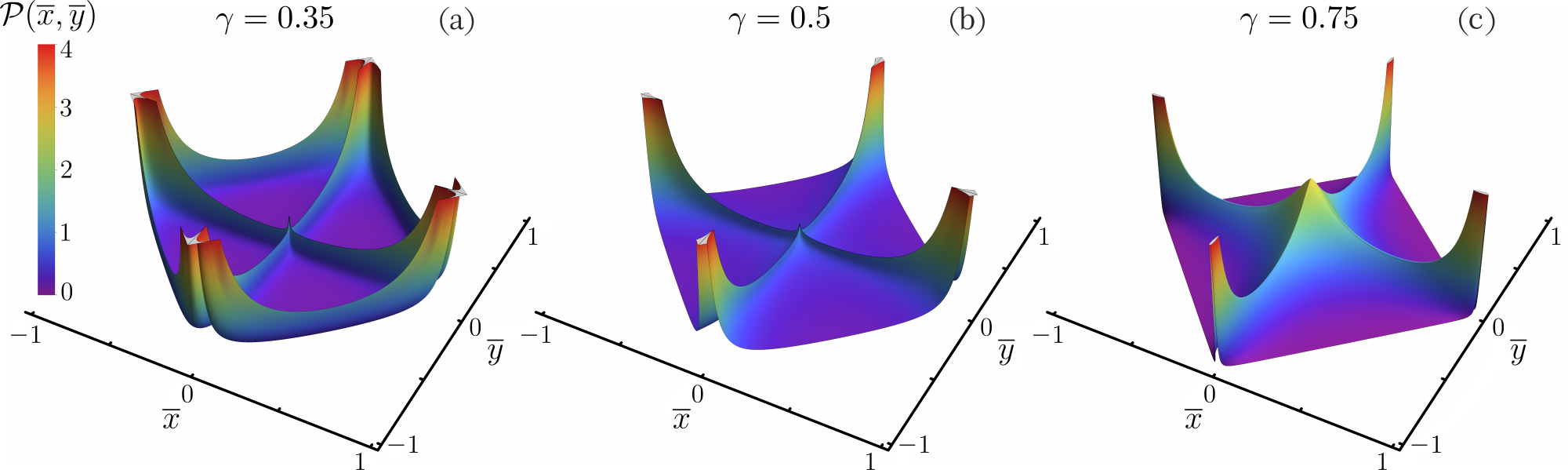
Figure 2: Asymptotic probability density functions $\mathcal{P}(\overline{x},\overline{y})$ for different values of $\gamma$. The functions are obtained by using Eq. (44). Note that in cases (a) and (b) $\mathcal{P}(\overline{x},\overline{y})$ is singular along lines $\overline{x}=0$ and $\overline{y}=0$, while minimal values of $\overline{x}$ and $\overline{y}$ used to plot the functions are $10^{-3}$. In the case (a), $\mathcal{P}(\overline{x},\overline{y})$ is also singular along the ballistic front $|x|+|y|=1$ and the outward points used to plot the functions are at distance $10^{-3}$ from the front.

From Eq. (26) we have

$$\mathcal{P}(\overline{x},\overline{y})=Q_{1}(\overline{x},\overline{y})+Q_{2}(\overline{x},\overline{y})+Q_{1}(\overline{y},\overline{x})+Q_{2}(\overline{y},\overline{x}),$$ (44)

where $Q_{1,2}(\overline{x},\overline{y})=Q_{1,2}(\overline{x},\overline{y},t=1)$. In Eqs. (27) and (28) we replace variable $\eta\mapsto\frac{1+\eta}{2}$. This allows us to extend the integration interval from $[0,1]$ to $[-1,1]$ and then implement Gauss–Jacobi quadrature RalstonRabinowitz . We chose this particular method because it is very convenient to deal numerically with integrals which includes power-law singularities.

We now write

$$Q_{1}(\overline{x},\overline{y}) =\int_{-1}^{1}\!\mathrm{d}\eta\,(1-\eta)^{\gamma-1}q_{1}(\eta;\overline{x},\overline{y}),$$ (45)

$$Q_{2}(\overline{x},\overline{y}) =\int_{-1}^{1}\!\mathrm{d}\eta\,(1-\eta)^{\gamma-1}q_{2}(\eta;\overline{x},\overline{y})$$ (46)

with functions

$$q_{1}(\eta;\overline{x},\overline{y}) =\frac{2(1-\gamma)}{\pi^{2}x_{r}^{\gamma-1}y_{r}(1-|\overline{x}|-|\overline{y}|)^{2}}(1-\eta)^{1-\gamma}\left(1-\eta+2x_{r}\right)^{\gamma-2}$$

$$\mathrel{\phantom{=}}\times\text{Re}\left\{\frac{1}{x_{r}^{-\gamma}\left[(1-\eta)^{\gamma}e^{i\pi\gamma}+(1-\eta+2x_{r})^{\gamma}\right]+y_{r}^{-\gamma}\left[(1+\eta)^{\gamma}e^{-i\pi\gamma}+(1+\eta+2y_{r})^{\gamma}\right]}\right.$$

$$\mathrel{\phantom{=}}-\left.\frac{1}{x_{r}^{-\gamma}\left[(1-\eta)^{\gamma}e^{i\pi\gamma}+(1-\eta+2x_{r})^{\gamma}\right]+y_{r}^{-\gamma}\left[(1+\eta)^{\gamma}e^{i\pi\gamma}+(1+\eta+2y_{r})^{\gamma}\right]}\right\},$$ (47)

$$q_{2}(\eta;\overline{x},\overline{y}) =\frac{2\gamma}{\pi^{2}x_{r}^{\gamma}y_{r}(1-|\overline{x}|-|\overline{y}|)^{2}}\left[x_{r}^{1-\gamma}\left(1-\eta+2x_{r}\right)^{\gamma-1}+y_{r}^{1-\gamma}\left(1+\eta+2y_{r}\right)^{\gamma-1}\right]$$

$$\mathrel{\phantom{=}}\times\text{Re}\left[e^{i\pi(\gamma-1)}+(1-\eta)^{1-\gamma}(1-\eta+2x_{r})^{\gamma-1}\right]$$

$$\mathrel{\phantom{=}}\times\left\{\frac{1}{\left\{x_{r}^{-\gamma}\left[(1-\eta)^{\gamma}e^{i\pi\gamma}+(1-\eta+2x_{r})^{\gamma}\right]+y_{r}^{-\gamma}\left[(1+\eta)^{\gamma}e^{-i\pi\gamma}+(1+\eta+2y_{r})^{\gamma}\right]\right\}^{2}}\right.$$

$$\mathrel{\phantom{=}}-\left.\frac{1}{\left\{x_{r}^{-\gamma}\left[(1-\eta)^{\gamma}e^{i\pi\gamma}+(1-\eta+2x_{r})^{\gamma}\right]+y_{r}^{-\gamma}\left[(1+\eta)^{\gamma}e^{i\pi\gamma}+(1+\eta+2y_{r})^{\gamma}\right]\right\}^{2}}\right\},$$ (48)

which have no singularities with respect to $\eta$ (for any fixed values of $\overline{x}$ and $\overline{y}$).

Following the Gauss–Jacobi quadrature recipe RalstonRabinowitz , we obtain

$$Q_{1}(\overline{x},\overline{y}) \approx\sum_{j=1}^{n}w_{j}q_{1}(\eta_{j};\overline{x},\overline{y}),$$ (49)

$$Q_{2}(\overline{x},\overline{y}) \approx\sum_{j=1}^{n}w_{j}q_{2}(\eta_{j};\overline{x},\overline{y}),$$ (50)

where weights are

$$w_{j} =-\frac{(2n+a+b+2)\Gamma(n+a+1)}{(n+a+b+1)^{2}\Gamma(n+a+b+1)}$$

$$\mathrel{\phantom{=}}\times\frac{\Gamma(n+b+1)2^{a+b+1}}{\Gamma(n+2)J_{n-1}^{(a+1,b+1)}(\eta_{j})J_{n+1}^{(a,b)}(\eta_{j})}$$ (51)

and $\eta_{j}$ are roots of Jacobi polynomials $J_{n}^{(a,b)}(\eta)$. In our case $a=\gamma-1$ and $b=0$.

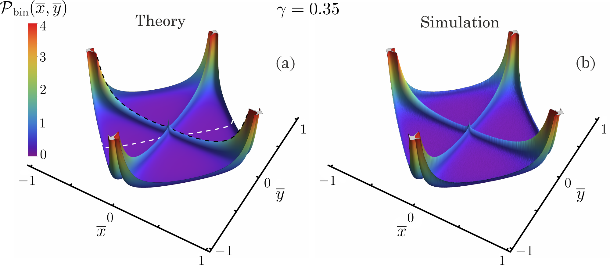
Figure 3: Averaged probability density functions $\mathcal{P}_{\mathrm{bin}}(\overline{x},\overline{y})$ for $\gamma=0.35$ obtained (a) with Eq. (54) and (b) by sampling a histogram for $t=10^{3}$ with $10^{8}$ realizations. To calculates the functions, the square $[-1,1]\times[-1,1]$ was divided into a grid of $400\times 400$ with cells. Sections $\overline{y}=0$ (black dashed line) and $\overline{y}=\overline{x}$ (white dashed line) are presented on Figures 5(a) and 6(a), respectively. Number of the sampled realisations is $10^{8}$.

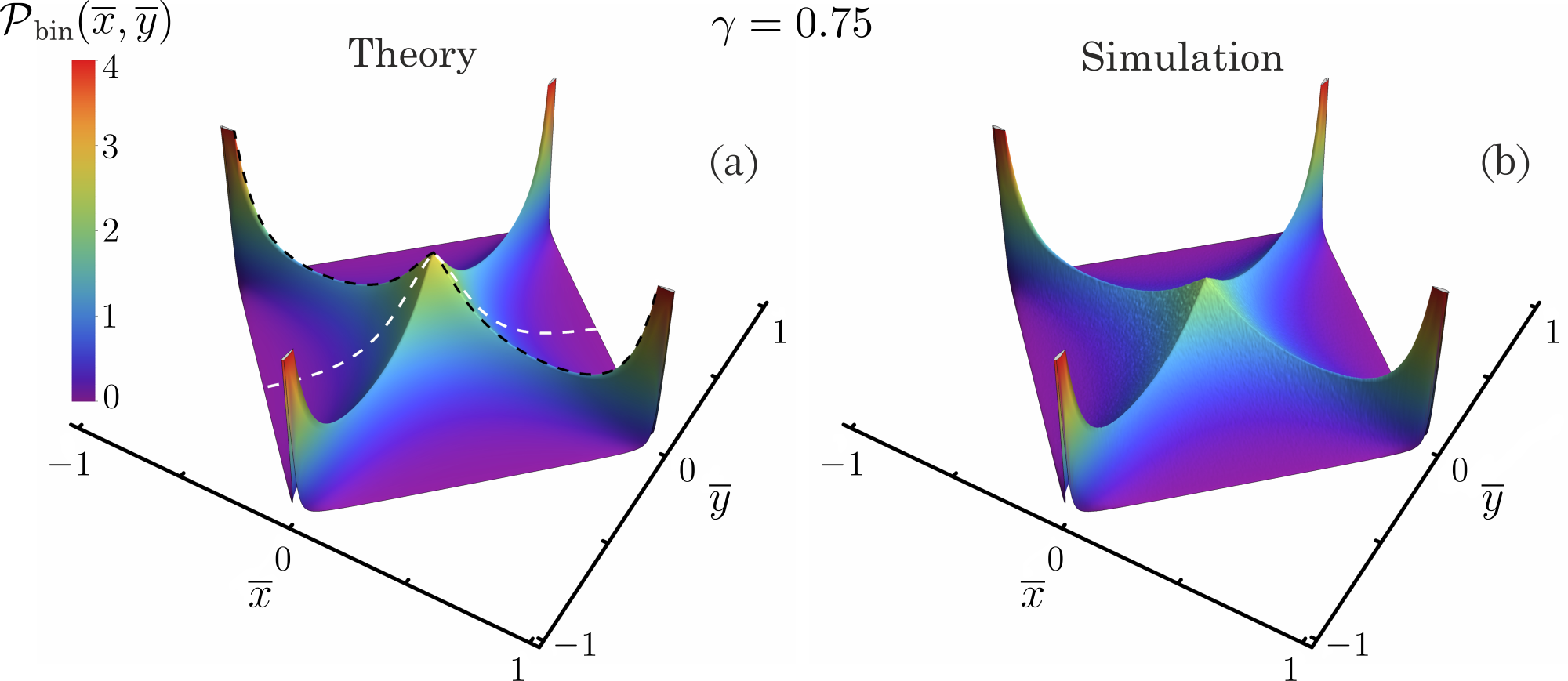
Figure 4: Averaged probability density functions $\mathcal{P}_{\mathrm{bin}}(\overline{x},\overline{y})$ for $\gamma=0.75$ obtained (a) with Eq. (54) and (b) by sampling a histogram for $t=10^{3}$ with $10^{8}$ realizations. To calculates the functions, the square $[-1,1]\times[-1,1]$ was divided into a grid of $400\times 400$ bins. Distributions along the sections $\overline{y}=0$ (black dashed line) and $\overline{y}=\overline{x}$ (white dashed line) are presented on Figures 5(c) and 6(c), respectively. Number of the sampled realisations is $10^{8}$.

In the functions under the integrals in Eqs. (45) and (46), we separate singular multiplier $(1-\eta)^{\gamma-1}$, and then compensate it with $(1-\eta)^{1-\gamma}$ in some places comment1 . Figure 2 shows asymptotic pdf computed for three different values of $\gamma$. Note that, for $\gamma=0.35$ and $0.5$, the corresponding pdf’s are singular along lines $\overline{x}=0$ and $\overline{y}=0$ to_be_published . Additionally, for $\gamma=0.35$, the pdf is also singular along the ballistic front to_be_published . The numerically calculated pdf’s have finite height because the minimal distances of the grid points from the singular lines are $10^{-3}$.

V.2 Comparison with the results of finite-time samplings

Here we discuss a procedure to compare analytical results with numerically sampled finite-time histograms.

We split the domain where the pdf takes non-zero values, i.e. inside the ballistic square $|\overline{x}|+|\overline{y}|<1$, into a set of bins.

Figure 5: Sections of $\mathcal{P}_{\mathrm{bin}}(\overline{x},\overline{y})$ along line $\overline{y}=\overline{y}_{0}=0$ for three different values of $\gamma$. Blue solid curves are theoretic results, red circles are result of the sampling for time $t=10^{3}$, and green stars [on panel (c)] are result of the sampling for time $t=10^{4}$. Number of the sampled realisations is $10^{8}$ in all the cases.

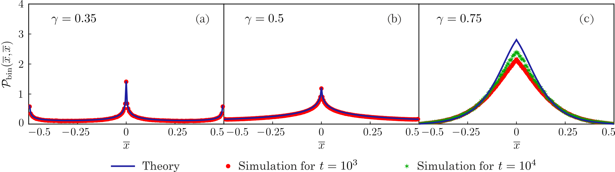
Figure 6: Sections of $\mathcal{P}_{\mathrm{bin}}(\overline{x},\overline{y})$ along line $\overline{y}=\overline{x}$ for three different values of $\gamma$. Blue solid curves are theoretic results, red circles are result of the sampling for time $t=10^{3}$, and green stars [on panel (c)] are result of the sampling for time $t=10^{4}$. Number of the sampled realisations is $10^{8}$ in all the cases.

Consider now bin $\mathcal{A}$ of area $S(\mathcal{A})$. Then the average probability density function over bin $\mathcal{A}$ is

$$\mathcal{P}_{\mathcal{A}}=\frac{1}{S(\mathcal{A})}\iint_{\mathcal{A}}\mathcal{P}(\overline{x},\overline{y})\mathrm{d}\overline{x}\mathrm{d}\overline{y}.$$ (52)

The corresponding pdf (which will be estimated through the numerical sampling) is

$$\mathcal{P}^{\mathrm{num}}_{\mathcal{A}}=\frac{1}{S(\mathcal{A})}\frac{N_{\mathcal{A}}}{N_{\mathrm{total}}}.$$ (53)

Here $N_{\mathcal{A}}$ is the number of realizations which ended up, after fixed time $t$, in bin $\mathcal{A}$, while $N_{\mathrm{total}}$ is the total number of realizations. Then, for large enough $N_{\mathrm{total}}$, we expect $\mathcal{P}_{\mathcal{A}}\approx\mathcal{P}^{\mathrm{num}}_{\mathcal{A}}$.

If function $\mathcal{P}(\overline{x},\overline{y})$ is continuous over $\mathcal{A}$, then, according to the mean value theorem, there is point $(\overline{x}_{c},\overline{y}_{c})\in\mathcal{A}$ such that $\mathcal{P}_{\mathcal{A}}=\mathcal{P}(\overline{x}_{c},\overline{y}_{c})$. If, in addition, $\mathcal{A}$ is small (compared to the characteristic scale over which $\mathcal{P}_{\mathcal{A}}$ varies substantially), then, by using Taylor series, we have $\mathcal{P}(\overline{x},\overline{y})\approx\mathcal{P}(\overline{x}_{c},\overline{y}_{c})$ for all $(\overline{x},\overline{y})\in\mathcal{A}$. Therefore, in a sufficiently small domain $\mathcal{A}$, pdf $\mathcal{P}(\overline{x},\overline{y})$ can be approximated by the average density over the domain such that $\mathcal{P}(\overline{x},\overline{y})|_{(\overline{x},\overline{y})\in\mathcal{A}}\approx\mathcal{P}_{\mathcal{A}}\approx\mathcal{P}^{\mathrm{num}}_{\mathcal{A}}$.

We partition the interior of square $|\overline{x}|+|\overline{y}|<1$ into set of bins with a set of lines parallel to the main Cartesian axes and distance $\varepsilon$ between two neighboring lines. By doing that, we obtain $M^{2}$ bins, $M=1/\varepsilon$.

Bin $\mathcal{A}_{ij}$ is defined as $\overline{x}_{i}\leq\overline{x}\leq\overline{x}_{i+1}$ and $\overline{y}_{j}\leq\overline{y}\leq\overline{y}_{j+1}$ with $\overline{x}_{i+1}-\overline{x}_{i}=\overline{y}_{j+1}-\overline{y}_{j}=\varepsilon$. We have

$$\mathcal{P}_{\mathcal{A}_{ij}} =\frac{1}{S(\mathcal{A}_{ij})}\iint_{\mathcal{A}_{ij}}\mathcal{P}(\overline{x},\overline{y})\mathrm{d}\overline{x}\mathrm{d}\overline{y}$$

$$=\frac{1}{\varepsilon^{2}}\int_{\overline{x}_{i}}^{\overline{x}_{i+1}}\!\int_{\overline{y}_{j}}^{\overline{y}_{j+1}}\mathcal{P}\!\left(\overline{x},\overline{y}\right)\mathrm{d}\overline{x}\mathrm{d}\overline{y}.$$

By introducing variables $\overline{x}=\frac{\overline{x}_{i+1}-\overline{x}_{i}}{2}x^{\prime}+\frac{\overline{x}_{i+1}+\overline{x}_{i}}{2}$ and $\overline{y}=\frac{\overline{y}_{j+1}-\overline{y}_{j}}{2}y^{\prime}+\frac{\overline{y}_{j+1}+\overline{y}_{j}}{2}$, which maps intervals $[\overline{x}_{i},\overline{x}_{i+1}]$ and $[\overline{y}_{j},\overline{y}_{j+1}]$ onto the interval $[-1,1]$, we get

$$\mathcal{P}_{\mathcal{A}_{ij}} =\frac{1}{4}\int_{-1}^{1}\!\int_{-1}^{1}\mathcal{P}\!\left[\frac{\varepsilon}{2}(x^{\prime}+1)+\overline{x}_{i},\frac{\varepsilon}{2}(y^{\prime}+1)+\overline{y}_{j}\right]\mathrm{d}x^{\prime}\mathrm{d}y^{\prime}$$

$$\approx\frac{1}{4}\sum_{m_{1}=1}^{m}\sum_{m_{2}=1}^{m}w_{m_{1}}w_{m_{2}}\mathcal{P}\!\left[\frac{\varepsilon}{2}(x^{\prime}_{m_{1}}+1)+\overline{x}_{i},\frac{\varepsilon}{2}(y^{\prime}_{m_{2}}+1)+\overline{y}_{j}\right]\!.$$ (54)

In the second line of Eq. (54) we approximate the integral by using orthogonal Legendre polynomials of order $m$ (they can be obtained as a particular case of Jacobi polynomials by setting $a=b=0$). Therefore, in this case weights $w_{m_{1},m_{2}}$ follows from Eq. (51) with $a=b=0$, while $x_{m_{1}}$ and $y_{m_{2}}$ are root of Legendre polynomial $P_{m}(\xi)=J_{m}^{(0,0)}(\xi)$. To find $\mathcal{P}_{\mathcal{A}_{ij}}$, we have to calculate $\mathcal{P}\!\left[\frac{\varepsilon}{2}(x^{\prime}_{m1}+1)+\overline{x}_{i},\frac{\varepsilon}{2}(y^{\prime}_{m2}+1)+\overline{y}_{j}\right]$ by using the above described method. For the bins ${A}_{ij}$, in which $\mathcal{P}(\overline{x},\overline{y})$ has singularities to_be_published , we can use the same scheme, by taking into account the corresponding singularity order in Eq. (54).

We denote the averaged (over the bin) probability density $\mathcal{P}_{\mathcal{A}_{ij}}$ as $\mathcal{P}_{\mathrm{bin}}(\overline{x},\overline{y})$, where $(\overline{x},\overline{y})$ are coordinates of the center of the corresponding bin $\mathcal{A}_{ij}$. To compare $\mathcal{P}_{\mathrm{bin}}(\overline{x},\overline{y})$ with $\mathcal{P}(\overline{x},\overline{y})$, we calculate pdf $\mathcal{P}(\overline{x},\overline{y})$ at the center of the corresponding bin $\mathcal{A}_{ij}$.

Figures 4–6 present a comparison of the probability distributions obtained by averaging pdf $\mathcal{P}(\overline{x},\overline{y})$, Eq. (30), over the bins of a $400\times 400$ grid, with the results of a finite-time sampling (by using the same grid) with $10^{8}$ realizations. While for $\gamma=0.35$ and $0.5$ sampling over time $t=10^{3}$ yields histograms that are in a perfect agreement with the theoretical results, for $\gamma=0.75$ the peak at the origin develops slowly in time.

VI Exact solution for $\gamma=1/2$

For $\gamma=1/2$ we have Lévy-Smirnov distribution SamorodnitskyTaqqu

$$\ell_{1/2}(t)=\frac{e^{-1/(4t)}}{2\sqrt{\pi}t^{3/2}}.$$

By substituting this into Eq. (43), after some elementary calculations, we obtain

$$\mathcal{P}(\overline{x},\overline{y})=\frac{4}{\pi^{2}(1-|\overline{x}|-|\overline{y}|)^{3}}\int_{0}^{1}\frac{\mathrm{d}\eta\sqrt{p(\eta)}}{\widetilde{p}^{2}(\eta)},$$

where

$$p(\eta)=(1+x_{r}-\eta)(1-\eta)\eta(\eta+y_{r})$$ (55)

and

$$\widetilde{p}(\eta)=p(\eta)\left(\frac{1}{1+x_{r}-\eta}+\frac{1}{1-\eta}+\frac{1}{\eta}+\frac{1}{\eta+y_{r}}\right).$$

Next, we take into account that

$$\widetilde{p}(\eta)=-(2+x_{r}+y_{r})(\eta-\eta_{1})(\eta-\eta_{2}),$$

where

$$\eta_{1,2}=\frac{1+x_{r}\pm\sqrt{(1+x_{r})(1+y_{r})(1+x_{r}+y_{r})}}{2+x_{r}+y_{r}}.$$ (56)

Since $1-|\overline{x}|-|\overline{y}|=\frac{2}{2+x_{r}+y_{r}}$ [as it follows from Eq. (42)], we can recast the expression for the asymptotic pdf in the form

$$\mathcal{P}(\overline{x},\overline{y})=\frac{2+x_{r}+y_{r}}{2\pi^{2}}\int_{0}^{1}\frac{\mathrm{d}\eta\sqrt{p(\eta)}}{(\eta-\eta_{1})^{2}(\eta-\eta_{2})^{2}}.$$ (57)

Because $p(\eta)$ is polynomial of the fourth order, the integral in Eq. (57) can be expressed through elliptic integrals Hancock (see Appendix B for more details):

$$\mathcal{P}(\overline{x},\overline{y}) =\Omega(\overline{x},\overline{y})\!\left[\left(\mu(\overline{x},\overline{y})+\frac{1}{\mu(\overline{x},\overline{y})}\right)K\!\left(1-\frac{1}{\mu^{2}(\overline{x},\overline{y})}\right)\right.$$

$$\mathrel{\phantom{=}}\left.-2\mu(\overline{x},\overline{y})E\!\left(1-\frac{1}{\mu^{2}(\overline{x},\overline{y})}\right)\right],$$ (58)

where

$$\Omega(\overline{x},\overline{y}) =\frac{(2+x_{r}+y_{r})^{3}}{16\pi^{2}}$$

$$\mathrel{\phantom{=}}\times\frac{\sqrt{(1+x_{r})(1+y_{r})}-\sqrt{1+x_{r}+y_{r}}}{(1+x_{r})(1+y_{r})(1+x_{r}+y_{r})},$$ (59)

$$\mu(\overline{x},\overline{y})=\frac{\sqrt{(1+x_{r})(1+y_{r})}+\sqrt{1+x_{r}+y_{r}}}{\sqrt{(1+x_{r})(1+y_{r})}-\sqrt{1+x_{r}+y_{r}}},$$ (60)

while $K(m)$ and $E(m)$ complete elliptic integrals of the first and second kind.

VII Conclusions

In this work we present a detailed theoretical analysis of a particular two-dimensional Lévy walk (LW) model in the ballistic regime. With this, we wanted to demonstrate that a complex planar spatially anisotropic LW process prl2016 can be evaluated analytically up to fine details asymptotics . In this context, our work constitutes a next step in the direction set in Refs. zarfaty1 ; zarfaty2 , where this program was realized for the border between diffusive and superdiffusive regimes, i.e., for $\gamma=2$.

The super-diffusive regime, $1<\gamma<2$, was partially addressed in Ref. fouxon2017 . This regime, however, is the hardest one to evaluate analytically. In this case $P(x,y,t)$ does not obey a uniform scaling but rather two different ones, a Lévy scaling governing the bulk of the pdf and co-variant scaling covariant governing the ballistic ends. In $2d$, aside of the obvious dependence of the scalings on the direction, the position of the ’meeting’ point of the two scalings depends not only on time (as in the one-dimensional case covariant ) but also on the direction. We hope that a progress will be made in this direction and it would be possible, f.e., to relate analytical considerations and numerical simulations of transport processes in two-dimensional Hamiltonian systems yosi3 .

VIII Acknowledgments

S.D. appreciate the hospitality of the Max Planck Institute for the Physics of Complex Systems (Dresden, Germany) where the project was finalized. He also acknowledges support by the Nord-STAR - Nordic Center for Sustainable and Trustworthy AI Research (OsloMet Project Code 202237-100).

Appendix A Inverse Fourier-Laplace transform in 1d case

Here we briefly review the method presented by Godrèche and Luck in Ref. GL2001 .

Assume there is scaling $G(x,t)=\frac{1}{t}\Phi\!\left(\frac{x}{t}\right)$. We denote $\overline{x}=\frac{x}{t}$ and obtain

$$G(k,s) =\mathcal{F}_{x}\mathcal{L}\{G(x,t)\}=\int_{-\infty}^{\infty}\frac{\Phi(\overline{x})\mathrm{d}\overline{x}}{ik\overline{x}+s}$$

$$=\frac{1}{s}\left\langle\frac{1}{1+\frac{ik}{s}\overline{X}}\right\rangle=\frac{1}{s}g\!\left(\frac{ik}{s}\right).$$ (61)

According to the Sokhotski–Plemelj theorem Vladimirov

$$\lim\limits_{\,\epsilon\rightarrow 0^{+}}\frac{1}{\xi\pm i\epsilon}=\mp i\pi\delta(\xi)+\mathscr{P}\frac{1}{\xi}$$

(a letter $\mathscr{P}$ denotes that the Cauchy principal value is taken) and, therefore, $\delta(\xi)\!=\!-\frac{1}{\pi}\text{Im}\!\lim\limits_{\epsilon\rightarrow 0^{+}}\frac{1}{\xi+i\epsilon}$.

Then, taking into account that

$$\Phi(\overline{x})=\langle\delta(\overline{x}-\overline{X})\rangle,$$ (62)

we obtain

$$\Phi(\overline{x}) =-\frac{1}{\pi}\text{Im}\!\lim\limits_{\,\epsilon\rightarrow 0^{+}}\left\langle\frac{1}{\overline{x}-\overline{X}+i\epsilon}\right\rangle$$

$$=-\frac{1}{\pi}\!\lim\limits_{\,\epsilon\rightarrow 0^{+}}\text{Im}\!\left[\frac{1}{\overline{x}+i\epsilon}g\!\left(-\frac{1}{\overline{x}+i\epsilon}\right)\right].$$ (63)

Therefore

$$G(x,t)=-\frac{1}{\pi x}\!\lim\limits_{\,\epsilon\rightarrow 0^{+}}\!\!\text{Im}\,g\!\left(-\frac{1}{x/t+i\epsilon}\right).$$ (64)

Next we show that the method proposed by Godrèche and Luck is related to the Stieltjes transform.

Namely, from Eq. (61) follows (here we introduce notation $ik/s=\zeta$)

$$g(\zeta)=\int_{-\infty}^{\infty}\frac{\Phi(\overline{x})\mathrm{d}\overline{x}}{1+\zeta\,\overline{x}}.$$

We make replace $\zeta=-1/z$ and obtain

$$\frac{1}{z}g\!\left(-\frac{1}{z}\right)=\int_{-\infty}^{\infty}\frac{\Phi(\overline{x})\mathrm{d}\overline{x}}{z-\overline{x}}.$$ (65)

The rhs of Eq. (65) is the Stieltjes transform of $\Phi(\overline{x})$. Denoting $\mathcal{S}(z)=\frac{1}{z}g\!\left(-\frac{1}{z}\right)$, taking into account that the inverse Stieltjes transform is defined as Widder

$$\Phi(\overline{x})=\lim\limits_{\,\epsilon\rightarrow 0^{+}}\!\frac{\mathcal{S}(\overline{x}-i\epsilon)-\mathcal{S}(\overline{x}+i\epsilon)}{2\pi i},$$

and using the identity $\text{Im}\,f=\frac{f-f^{*}}{2i}$, we arrive at the formula (63).

Therefore, it is clear now that the method, in principle, is a particular case of the implementation of the inverse Stieltjes transform. Usually it is used for the probability density functions. However, it is not specific and can be used for general functions Widder , like functions in Eqs. (13) and (14).

Appendix B Legendre’s normal form for elliptic integrals

Assume that $R(\eta)$ is a forth-order polynomial and $S(\eta)$ is an arbitrary rational function. We will follow Ref. Hancock (Section VIII in there), and describe a method to reduce integrals of the following type

$$I=\int_{0}^{1}\frac{S(\eta)\mathrm{d}\eta}{\sqrt{R(\eta)}}$$ (66)

to elliptic ones. We are only interested in the case when all roots of $R(\eta)$ are real; we also set the leading coefficient of the polynomial equals to one. We write $R(\eta)=(\eta-a_{1})(\eta-a_{2})(\eta-a_{3})(\eta-a_{4})$ and apply to Eq. (66) the following linear fractional transform

$$\eta=\frac{a\omega+b}{c\omega+d},$$ (67)

where we also assume $ad-bc\neq 0$. Next we take into account that

$$\eta-a_{j}=\frac{(a-ca_{j})\omega+b-da_{j}}{c\omega+d}$$

with $j=\overline{1,4}$ and

$$\mathrm{d}\eta=\frac{ad-bc}{(c\omega+d)^{2}}\mathrm{d}\omega,$$

and arrive at

$$I=\int_{-\frac{b}{a}}^{-\frac{b-d}{a-c}}\frac{(ad-bc)\sigma(\omega)\mathrm{d}\omega}{\sqrt{\prod\limits_{j=1}^{4}[(a-ca_{j})\omega+b-da_{j}]}},$$ (68)

where $\sigma(\omega)=S\!\left(\frac{a\omega+b}{c\omega+d}\right)$ is a rational function.

Next we write

$$\prod\limits_{j=1}^{4}[(a-ca_{j})\omega+b-da_{j}] =(q_{0}\omega^{2}+q_{1}\omega+q_{2})$$

$$\mathrel{\phantom{=}}\times(h_{0}\omega^{2}+h_{1}\omega+h_{2})$$ (69)

with coefficients

$$q_{0} =(a-ca_{1})(a-ca_{2}),$$

$$q_{1} =(a-ca_{1})(b-da_{2})+(a-ca_{2})(b-da_{1}),$$

$$q_{2} =(b-da_{1})(b-da_{2}),$$

$$h_{0} =(a-ca_{3})(a-ca_{4}),$$

$$h_{1} =(a-ca_{3})(b-da_{4})+(a-ca_{4})(b-da_{3}),$$

$$h_{2} =(b-da_{3})(b-da_{4}).$$

We choose $a,b,c,d$ such that in polynomial (69) coefficients for $\omega^{3}$ and $\omega$ are nullified. Whence it follows conditions

$$q_{0}h_{1}+h_{0}q_{1}=0,\quad q_{1}h_{2}+h_{1}q_{2}=0,$$

which hold for $q_{1}=h_{1}=0$.

We obtain therefore a system of equations:

$$2-\left(\frac{d}{b}+\frac{c}{a}\right)(a_{1}+a_{2})+2\frac{d}{b}\frac{c}{a}a_{1}a_{2}=0,$$

$$2-\left(\frac{d}{b}+\frac{c}{a}\right)(a_{3}+a_{4})+2\frac{d}{b}\frac{c}{a}a_{3}a_{4}=0,$$ (70)

from which the expressions for $\frac{d}{b}+\frac{c}{a}$ and $\frac{d}{b}\frac{c}{a}$ can be obtained. From four variables $a,b,c,d$ we can choose two as parameters and solve the system of equations for the remaining two. Integral in Eq. (68) can be written now as

$$I=\int_{-\frac{b}{a}}^{-\frac{b-d}{a-c}}\frac{(ad-bc)\sigma(\omega)\mathrm{d}\omega}{\sqrt{(q_{0}\omega^{2}+q_{2})(h_{0}\omega^{2}+h_{2})}},$$ (71)

and can be reduced to a combination of elliptic integrals of the first, second, and third orders Hancock .

We apply the above described approach to the integral in Eq. (57)

$$I=\int_{0}^{1}\frac{\mathrm{d}\eta}{\sqrt{p(\eta)}}\frac{p(\eta)}{(\eta-\eta_{1})^{2}(\eta-\eta_{2})^{2}}.$$ (72)

We set $R(\eta)=p(\eta)$, $S(\eta)=\frac{p(\eta)}{(\eta-\eta_{1})^{2}(\eta-\eta_{2})^{2}}$ and

$$a_{1}=1+x_{r},\quad a_{2}=1,\quad a_{3}=0,\quad a_{4}=-y_{r}.$$

After applying the linear fractional transform (67) with parameters $a=-1$ and $b=1$ (just a convenient choice), we get solutions of the system (70):

$$c =\frac{1+x_{r}+\sqrt{D}}{(1+x_{r})y_{r}},\quad d=-\frac{1+x_{r}-\sqrt{D}}{(1+x_{r})y_{r}},$$

$$c =\frac{1+x_{r}-\sqrt{D}}{(1+x_{r})y_{r}},\quad d=-\frac{1+x_{r}+\sqrt{D}}{(1+x_{r})y_{r}},$$ (73)

where

$$D=(1+x_{r})(1+y_{r})(1+x_{r}+y_{r}).$$ (74)

It is not important which pair to choose; we take the second one form Eq. (73), which guarantees $ad-bc>0$.

Thus, we get

$$ad-bc =\frac{2\sqrt{D}}{(1+x_{r})y_{r}},\quad-\frac{b}{a}=1,$$

$$-\frac{b-d}{a-c} =\frac{(1+x_{r})(1+y_{r})+\sqrt{D}}{(1+x_{r})(1+y_{r})-\sqrt{D}},$$

and

$$q_{0,2} =\frac{\left(1+x_{r}+y_{r}\mp\sqrt{D}\right)\!\left[(1+x_{r})(1+y_{r})\mp\sqrt{D}\right]}{(1+x_{r})y_{r}^{2}},$$

$$h_{0,2} =\pm\frac{\sqrt{D}}{1+x_{r}}.$$ (75)

After substituting (67) and taking into account the above results, we arrive at

$$p(\eta)=\frac{(q_{0}\omega^{2}+q_{2})(h_{0}\omega^{2}+h_{2})}{(c\omega+d)^{4}},$$

$$q_{0}\omega^{2}+q_{2} =|q_{0}|\left(\frac{q_{2}}{|q_{0}|}-\omega^{2}\right),$$

$$h_{0}\omega^{2}+h_{2} =h_{0}(\omega^{2}-1),$$

$$\eta-\eta_{1} =\frac{2}{c\omega+d}\frac{(1+y_{r})(1+x_{r}+y_{r})+\sqrt{D}}{(2+x_{r}+y_{r})y_{r}},$$

$$\eta-\eta_{2} =-\frac{2}{c\omega+d}\frac{(1+y_{r})(1+x_{r}+y_{r})-\sqrt{D}}{(2+x_{r}+y_{r})y_{r}}\omega,$$

$$\sigma(\omega) =\frac{(2+x_{r}+y_{r})^{2}y_{r}^{2}}{16(1+y_{r})^{2}(1+x_{r}+y_{r})^{2}}|q_{0}|h_{0}$$

$$\mathrel{\phantom{=}}\times\left(-\omega^{2}+\frac{q_{2}}{|q_{0}|}+1-\frac{q_{2}}{|q_{0}|\omega^{2}}\right).$$

Here we took into account that $q_{0}<0$, $h_{2}<0$ and $h_{2}=-h_{0}$. Reducing Eq. (71), we get

$$I =\theta\int_{1}^{\mu}\frac{\mathrm{d}\omega}{\sqrt{\left(\frac{q_{2}}{|q_{0}|}-\omega^{2}\right)\!\left(\omega^{2}-1\right)}}$$

$$\mathrel{\phantom{=}}\times\left(-\omega^{2}\!+\!\frac{q_{2}}{|q_{0}|}+1-\frac{q_{2}}{|q_{0}|\omega^{2}}\right)\!,$$ (76)

where

$$\theta =\frac{(2+x_{r}+y_{r})^{2}}{8D}$$

$$\mathrel{\phantom{=}}\times\left[\sqrt{(1+x_{r})(1+y_{r})}-\sqrt{1+x_{r}+y_{r}}\right],$$ (77)

$$\mu=-\frac{b-d}{a-c}=\frac{(1+x_{r})(1+y_{r})+\sqrt{D}}{(1+x_{r})(1+y_{r})-\sqrt{D}}.$$ (78)

From Eq. (75) we obtain

$$\frac{q_{2}}{|q_{0}|}=\frac{\left[\sqrt{D}+1+x_{r}+y_{r}\right]\!\left[(1+x_{r})(1+y_{r})+\sqrt{D}\right]}{\left[\sqrt{D}-(1+x_{r}+y_{r})\right]\!\left[(1+x_{r})(1+y_{r})-\sqrt{D}\right]}.$$

Next we use Eq. (74) and identity

$$\frac{\lambda_{1}+\sqrt{\lambda_{1}\lambda_{2}}}{\lambda_{1}-\sqrt{\lambda_{1}\lambda_{2}}}=\frac{\sqrt{\lambda_{1}\lambda_{2}}+\lambda_{2}}{\sqrt{\lambda_{1}\lambda_{2}}-\lambda_{2}},$$

and find out

$$\frac{(1+x_{r})(1+y_{r})+\sqrt{D}}{(1+x_{r})(1+y_{r})-\sqrt{D}}=\frac{\sqrt{D}+1+x_{r}+y_{r}}{\sqrt{D}-(1+x_{r}+y_{r})}.$$

Therefore, the following holds

$$\mu=\frac{\sqrt{D}+1+x_{r}+y_{r}}{\sqrt{D}-(1+x_{r}+y_{r})},\quad\frac{q_{2}}{|q_{0}|}=\mu^{2}.$$ (79)

Integral (76) takes a form

$$I=\theta\int_{1}^{\mu}\frac{\mathrm{d}\omega}{\sqrt{\left(\mu^{2}-\omega^{2}\right)\left(\omega^{2}-1\right)}}\left(-\omega^{2}+\mu^{2}+1-\frac{\mu^{2}}{\omega^{2}}\right).$$

It is easy to see that $-\omega^{2}+\mu^{2}+1-\frac{\mu^{2}}{\omega^{2}}\geq 0$ for $\omega\in[1,\mu]$, and therefore $I>0$.

Finally, by using table integrals Prudnikov , we get

$$I=\theta\left[\left(\mu+1/\mu\right)K\!\left(1\!-\!1/\mu^{2}\right)-2\mu E\!\left(1\!-\!1/\mu^{2}\right)\right]\!,$$ (80)

where

$$K(m) =\int_{0}^{\pi/2}\frac{\mathrm{d}\varphi}{\sqrt{1-m\sin^{2}\!\varphi}},$$ (81)

$$E(m) =\int_{0}^{\pi/2}\mathrm{d}\varphi\sqrt{1-m\sin^{2}\!\varphi}$$ (82)

are complete elliptic integrals of the first and second orders, respectively. It is noteworthy that Eq. (80) can be recast by using the hypergeomtric functions, by using $K(m)=\frac{\pi}{2}{}_{2}F_{1}\left(\frac{1}{2},\frac{1}{2};1;m\right)$ and $E(m)=\frac{\pi}{2}{}_{2}F_{1}\left(-\frac{1}{2},\frac{1}{2};1;m\right)$.

References

- (1) M. F. Shlesinger, J. Klafter, and Y. Wong, Random walks with infinite spatial and temporal moments, J. Stat. Phys. 27, 499 (1982).
- (2) M. F. Shlesinger, B. J. West, and J. Klafter, Lévy dynamics of enhanced diffusion: applications to turbulence, Phys. Rev. Lett. 58, 1100 (1987).
- (3) V. Zaburdaev, S. Denisov, J. Klafter, Lévy walks, Rev. Mod. Phys. 87, 483 (2015).
- (4) V. Zaburdaev, I. Fouxon, S. Denisov, and E. Barkai, Superdiffusive dispersals impart the geometry of underlying random walks, Phys. Rev. Lett. 117, 270601 (2016).
- (5) M. Magdziarz and T. Zorawik, Explicit densities of multidimensional ballistic Lévy walks, Phys. Rev. E 94, 022130 (2016).
- (6) M. Magdziarz and T. Zorawik, Method of calculating densities for isotropic ballistic Lévy walks, Commun. Nonlinear Sci. Numer. Simul. 48, 462 (2017).
- (7) I. Fouxon, S. Denisov, V. Zaburdaev, and E. Barkai, Limit theorems for Lévy walks in dimensions: rare and bulk fluctuations, J. Phys. A: Math. Theor. 50, 154002 (2017).
- (8) J. Klafter and G. Zumofen, Lévy statistics in a Hamiltonian system, Phys. Rev. E 49, 4873 (1994).
- (9) L. van der Heijdt, Face to Face with Dice: 5000 Years of Dice and Dicing (Gopher Publishers, Groningen, 2002).
- (10) L. Zarfaty, A. Peletskyi, I. Fouxon, S. Denisov, and E. Barkai, Dispersion of particles in an infinite-horizon Lorentz gas, Phys. Rev. E 98, 010101 (2018).
- (11) G. Cristadoro, T. Gilbert, M. Lenci, and D. P. Sanders, Measuring logarithmic corrections to normal diffusion in infinite-horizon billiards, Phys. Rev. E 90, 022106 (2014).
- (12) L. Zarfaty, A. Peletskyi, E. Barkai, and S. Denisov, Infinite horizon billiards: Transport at the border between Gauss and Lévy universality classes, Phys. Rev. E 100, 042140 (2019).
- (13) D. Froemberg, M. Schmiedeberg, E. Barkai, and V. Zaburdaev, Asymptotic densities of ballistic Lévy walks, Phys. Rev. E 91, 022131 (2015).
- (14) M. M. Meerschaert, D. A. Benson, H.-P. Scheffler, and P. Becker-Kern, Governing equations and solutions of anomalous random walk limits, Phys. Rev. E 66, 060102(R) (2002).
- (15) I. M. Sokolov and R. Metzler, Towards deterministic equations for Lévy walks: The fractional material derivative, Phys. Rev. E 67, 010101 (2003).
- (16) R. Metzler and J. Klafter, The restaurant at the end of the random walk: Recent developments in the description of anomalous transport by fractional dynamics, J. Phys. A: Math. Gen. 37, R161 (2004).
- (17) C. Godrèche and J. M. Luck, Statistics of the occupation time of renewal processes, J. Stat. Phys. 104, 489 (2001).
- (18) G. Samorodnitsky and M. S. Taqqu, Random Processes: Stochastic Models with Infinite Variance Stable Non-Gaussian (Chapman and Hall, NY, 1994).
- (19) H. Hancock, Lectures on the Theory of Elliptic Functions. Vol. I (John Wiley & Sons Inc., NY, 1910).
- (20) Formally, and . However, since variables and are related to the expression which does not depend on explicitly, we use different notations here to distinguish these two different situations.
- (21) A. Ralston, P. Rabinowitz, A First Course in Numerical Analysis (Dover Publ. Inc., NY, 2001).
- (22) An alternative is to split expression in Eq. (45) into summands of two different types, which do and do not include singular multiplier . However, in this case we would need two different types of orthogonal polynomials; e.g., for weights and nodes .
- (23) Yu. S. Bystrik and S. Denisov, in preparation.
- (24) D. V. Widder, The Laplace Transform (Princeton University Press, 1946).
- (25) A. P. Prudnikov, Yu. A. Brychkov, and O. I. Marichev, Integrals and Series, Volume 1: Elementary Functions (Taylor & Francis, London, 2002).
- (26) V. S. Vladimirov, Equations of Mathematical Physics (Dekker, NY, 1971).
- (27) Sections of the asymptotic pdf’s along different directions can be evaluated analytically and, e.g., for , two singularities going along the axes, power-law and logarithmic ones, can be distinguished to_be_published .
- (28) A. Rebenshtok, S. Denisov, P. Hänggi, and E. Barkai, Non-normalizable densities in strong anomalous diffusion: Beyond the central limit theorem, Phys. Rev. Lett. 112, 110601 (2014).