Eigenvalues of Autocovariance Matrix: A Practical Method to Identify the Koopman Eigenfrequencies
Abstract
To infer eigenvalues of the infinite-dimensional Koopman operator, we study the leading eigenvalues of the autocovariance matrix associated with a given observable of a dynamical system. For any observable for which all the time-delayed autocovariance exist, we construct a Hilbert space and a Koopman-like operator that acts on . We prove that the leading eigenvalues of the autocovariance matrix has one-to-one correspondence with the energy of that is represented by the eigenvectors of . The proof is associated to several representation theorems of isometric operators on a Hilbert space, and the weak-mixing property of the observables represented by the continuous spectrum. We also provide an alternative proof of the weakly mixing property. When is an observable of an ergodic dynamical system which has a finite invariant measure , coincides with closure in of Krylov subspace generated by , and coincides with the classical Koopman operator. The main theorem sheds light to the theoretical foundation of several semi-empirical methods, including singular spectrum analysis (SSA), data-adaptive harmonic analysis (DAHD), Hankel DMD and Hankel alternative view of Koopman analysis (HAVOK). It shows that, when the system is ergodic and has finite invariant measure, the leading temporal empirical orthogonal functions indeed correspond to the Koopman eigenfrequencies. A theorem-based practical methodology is then proposed to identify the eigenfrequencies of from a given time series. It builds on the fact that the convergence of the renormalized eigenvalues of the Gram matrix is a necessary and sufficient condition for the existence of eigenfrequencies. Numerical illustrating results on simple low dimensional systems and real interpolated ocean sea-surface height data are presented and discussed.
I Introduction
The dynamic mode decomposition (DMD) algorithm, is a powerful and versatile data-driven approach proposed by [1], ideally suited to analyze complex high-dimensional geophysical flows in terms of recurrent or quasi-periodic modes. The DMD is indeed related to the Koopman theory [2], stating that observables of an Hamiltonian system can always be described via a linear transformation. The original DMD algorithm has a lot of common points with the algorithm presented in [3]. For practical applications and real data analysis, several follow-up algorithms have been proposed. To name a few, it can be listed the optimized DMD [4], the optimal mode decomposition [5], the exact DMD[6], the Hankel DMD [7], the sparsity promoting DMD [8], the multi-resolution DMD [9], the extended DMD [10], DMD with control [11], total least squares DMD [12], dynamic distribution decomposition [13], etc. These DMD algorithms are generally motivated by different reasons, but a key overall objective is to help provide the most precise numerical approximation of the Koopman operator. When the system is ergodic and measure-preserving, it would indeed be equivalent to have a precise description of the spectrum of Koopman operator restricted on and a precise mapping between and (where is the linear subspace generated by a single observable and the unit complex circle, see section 2 for detailed definition of these spaces). The authors of [14] proved the convergence in the strong operator topology of extended DMD algorithm, provided a complete orthogonal basis of the space of square-integrable observables. In [7] the convergence of Hankel DMD algorithm is proved for the finite dimensional case, which corresponds to the finite truncation of the discrete part of the spectrum. Christoffel-Darboux kernel is exploited in [15] to directly identify the discrete component and the absolutely continuous component of the spectrum. Note, DMD algorithms are not the only way to approximate Koopman operator. In a series of papers ( [16],[17], [18],[19] and [20]), the approximation of Koopman operator is performed by kernel methods. Recently, [20] showed the convergence of kernel methods for any measure preserving ergodic dynamical systems, the measure of which support lies on a compact manifold. A related issue for stochastic dynamics can be found in [21]
In this manuscript, we define a Hilbert space and the associated Koopman-like time-shift operator for each given time series the autocovariances of which exist. When the time series is given by an observable on a ergodic dynamical system with finite invariant measure, coincides with the closure of the infinite dimensional Krylov subspace generated by the classical Koopman operator and , and coincides with the classical Koopman operator on . We argue and prove that for any observable such that all the time-delayed autocovariance exist, when the parameters of the autocovariance matrix goes to infinity in the right order, the leading eigenvalues renormalized by the dimension of converge to the energy of that is represented by the eigenvector of . All other renormalized eigenvalues shall further converge to 0 uniformly. Despite its theoretical interests, the main theorem directly suggests a practical algorithm to explicitly identify the Koopman eigenfrequencies together with the associated energy from given time series. As a by-product, it also shows that the leading temporal empirical orthogonal functions calculated by singular spectrum analysis (SSA, [22]) method are indeed represented by the eigenfrequencies of . Similarly, this theorem also sheds light on the theoretical foundation of data-adaptive harmonic decomposition (DAHD,[23], and Hankel alternative view of Koopman analysis (HAVOK, [24]). Because all these methods are based either on trajectory matrix or on .
The paper is organized as follows. In section 2, we present our main result and the necessary mathematical background knowledge. We also discuss about how the main theorem provides theoretical support to SSA,DAHD, and HAVOK. In section 3, we state the details of the proof of the main result. In section 4, we present the detailed algorithm and compare it with another numerical method based on Yosida’s mean ergodic theorem ([25]). In section 5 we present numerical results on two simple low dimensional measure preserving ergodic dynamical systems and interpolated ocean sea-surface height data. Section 6 concludes this study and gives some perspectives. The necessary code and data that reproduces all the numerical results can be accessed at https://doi.org/10.5281/zenodo.5585970.
II Preliminaries and the main result
Given a continuous-time dynamical system
and an observable , we have a time series . We assume that the time-delayed autocovariance of exists for all :
| (1) |
To avoid misinterpretation, we use to denote time series associated to and a given (fixed) orbit of the dynamical system. For , we define to be the time shifted time series . For any and any two time series, associated to the same dynamics
we define
Let
| (2) |
Then is a linear space. Now we define the Koopman-like (or time shift) operator on . We start with for any
| (3) |
and then generalize the action of to the whole . It is not hard to show that is well-defined.
The existence of allows us to define an inner product on by
| (4) |
where . For any , it is obvious that
| (5) |
Hence preserves the inner product in and is hence continuous.
Let be the completion of . is a Hilbert space. preserves the inner product of . Therefore can be extended, by continuity, to an isometric operator that acts on . For sake of simplicity, keeping the same notation for the extended operator, , whose domain is , is the Koopman-like (or time shift) operator we study in this paper.
Remark 1.
The classical Koopman operator is defined to act on some function space on the whole phase space of some dynamical system, i.e.
| (6) |
where is a state and the discrete-time flow of the dynamical system.
In our setting, the definition of and purely relies on the time series. The dynamical system is hidden behind. It is possible that the time series only reveals partial properties of the dynamical system. When the discrete-time dynamical system is ergodic and has finite invariant measure , Birkhoff ergodic theorem guarantees that is isomorphic to the closure of Krylov subspace as Hilbert spaces. The isomorphism is given by
| (7) |
And it is not hard to see that acts on in a similar way as on the space of observables , i.e. for any ,
| (8) |
The elements in can always be represented as some time series. But in general we can not assert that any element in can be represented as some time series. In particular, we do not know if the eigenvectors of can be represented as a time series in the form . Nor in general can we identify with some space of functions on the phase space. Hence, without these assumptions, the time-shift operator and the Koopman operator cannot be strictly related. Ergodicity+finite invariant measure is a stronger assumption than the existence of autocovariance. As long as the autocovariances exist, the quantities mentioned in the main result are mathematically well-defined. Therefore we do not restrict ourselves to the case where the system is ergodic and has finite invariant measure. But we keep the generality in the definition of and . The physical meaning of and in the general case needs to be studied further. For readers who are interested in the classical Koopman operator , we point out that indeed coincides with when the system is ergodic and has finite invariant measure.
If is a continuous-time time series, we assume that
| (9) |
exists for every . Similar to the discrete-time case, we define
| (10) |
to be the continuous time series that starts from . We can define the linear space
| (11) |
with inner product:
| (12) |
Let be the completion of . is an isometry on for all .
We are interested in the eigenvalues and eigenvectors of (for discrete-time case) and (for continuous-time case). A natural question to ask is that whether the eigenfrequencies of and are the same. We have the following result.
Proposition 1.
Let be a continuous time process for which exists for all . Assume that the curve is continuous in . Let be a time step. Assume that
| (13) |
then . Let be an eigenfrequency of the discrete-time operator , i.e. there exists so that . Then there exists an integer , and , so that
| (14) |
for all .
The proof of this proposition is given in the appendix. Proposition 1 guarantees that for every eigenfrequency of , there always exists an eigenfrequency of for all which reduces to at discrete time step.
Our discussion about continuous-time time series stops here. Hereinafter we always assume that the time series is discrete in time. For simplicity the time series is denoted by and we use to denote the whole time series generated by as an element in . We use the notation to replace . Recall that the time-shift operator is an isometry on the Hilbert space of time-series associated to observable .
Remark 2.
Due to Birkhoff ergodic theorem, autocovariance exists when the dynamical system is ergodic and has a finite invariant measure.
The following theorem provides a very useful result to decompose any isometric operator and the Hilbert space on which it acts into unitary and non unitary part.
Theorem 1 (Wold decomposition).
Let be a Hilbert space and any isometry of . Then we have an orthogonal decomposition , and , such that , acts on for some index set as a unilateral shift, i.e. . And acts on and is unitary. is called the completely non unitary part of as it does not contain closed subspaces of on which acts as a unitary operator.
Wold theorem is a particular case of (Szökefalvi-Nagy–Foia s) theorem for contraction operator.
Theorem 2 (Szökefalvi-Nagy–Foias).
Let be a contraction operator (i.e. ) on a Hilbert space then
is the largest space among all closed -invariant and -invariant subspaces of H on which restricts to a unitary operator. The orthogonal complement is the completely non unitary part of . Here fix(A) refers to the subspace spanned by all the invariant vectors of operator .
Theorem 1 implies an orthogonal decomposition . Note that and are invariant under and . Then the fact that is generated by implies that . Note that for any eigenvector of associated to eigenvalue , we have an orthogonal decomposition , where , . Then . Because and are invariant subspaces, is an orthogonal decomposition for which , , implying that and are both eigenvectors of the same eigenvalue. must be zero because acts on as the unilateral shift operator. Hence a eigenvector must be inside .
Definition 1.
A Hilbert space with an unitary operator is called -cyclic if for some .
Theorem 3 (Spectral theorem for unitary operator).
Let be a Hilbert space and an unitary operator on . Assume that is -cyclic for some . Then there exists a finite measure on the unit circle , and an isomorphism
| (15) |
such that , for any and any . In particular, .
See lemma 5.4 in [26] for a mathematical proof. Note that lemma 5.4 in [26] assumes that , which is a weaker assumption than being cyclic in the sense of Definition 1. Therefore Theorem 3 applies to and . In general, the spectrum measure consists of the discrete component, the singular-continuous component, and the absolutely continuous component (with respect to Lebesgue measure): . The three components are pairwise-orthogonal, in the sense that for any , we can write such that , , similarly for and . Together with theorem 1, this suggests the orthogonal decomposition , and
| (16) |
It is easy to see that and are invariant subspaces of . In particular, the discrete part is a finite or countable sum of Dirac measures , where is the support of . Hence we can write
| (17) |
where if and 0 otherwise.
As such, for every , is an eigenvector of . On the other hand, let be an eigenvector of , i.e. for some . Then . Let , then , meaning that in . Hence , and . This shows that there is a one-to-one correspondence between the support of the discrete measure and the eigenvectors inside . In particular, all the eigenvectors of are simple.
Let be the corresponding normalized eigenvectors, then we have
| (18) |
Our goal is to evaluate , the numerical tool is the Gram matrix , where the entry is
| (19) |
We also define the autocovariance matrix
It is obvious that for any
| (20) |
Recall that and that each of these four components is orthogonal to all other components. Hence
| (21) |
Let be the eigenvalues of . Let be the eigenvalues of . It is clear that
| (22) |
Our main result states that:
Theorem 4 (Main result).
Assume that the autocovariance exists for all . Let be the time shift operator eigenvectors of unit length. Let the Hilbert space of observable time-series with , where and are the components of in the space spanned by the singular-continuous spectrum and absolute-continuous spectrum, and the component of in the completely non unitary subspace (i.e. direct sum of unilateral shift spaces). Assume that . Then for any :
| (23) |
For a given observable , the trajectory matrix is defined as:
| (24) |
Then it is clear that
| (25) |
where refers to the conjugate transpose of . Let be the singular values of . Then directly we have that .
Corollary 1 (Trajectory matrix version).
Assume exists for all . Then
| (26) |
Remark 3.
The Gramian matrix is used by singular spectrum analysis methods ([22]) to construct temporal modes of the given time series. The eigenfunctions of are called temporal empirical orthogonal functions (EoFs). Theorem 4 implies that the leading temporal EoFs are due to theoretical eigenfrequencies of . Similarly, the data-adaptive harmonic decomposition (DAHD, [23]) and Hankel alternative view of Koopman analysis (HAVOK, [24]) are based on Gramian matrix and trajectory matrix, respectively. The main theorem and the corollary directly provides a way to identify which features extracted by SSA, DAHD, or HAVOK are related to eigenfrequencies of , and which features are not.
The main result can be summarized as the following abstract mathematical theorem with respect to isometric operators Hilbert space. According to our knowledge, this mathematical result is not shown in any previous literature.
Theorem 5 (Main result in pure mathematical form).
Let be a Hilbert space and an isometry of . The inner product in is denoted by . Let be any vector. Let
| (27) |
Let be the eigenvectors of in . And let
| (28) |
be the decomposition of , where is perpendicular to the subspace spanned by all the eigenvectors of . There maybe uncountably many in but only countably many are included in the summation. Let be the eigenvalues of . And assume that . Then
| (29) |
III Proof of the main theorem
We first present several lemmas which are independent of the language of Koopman theory.
Lemma 1.
Let be a contraction on a Hilbert space . Then for every
Proof of lemma 1.
For every the sequence is decreasing thus convergent. For any , we have
Hence for every as , therefore,
The same argument for yields
as .
We obtain that as for every
∎
Lemma 2.
Let be a Hilbert space over of finite dimension or infinite dimension. such that . Then
| (30) |
Proof of Lemma 2.
Without loss of generality, we may assume that . For any , there exists such that . Further there exists , such that for any and , . Now for any ,
| (31) | ||||
∎
Lemma 3 (The weakly mixing property).
Let be a continuous measure on . Then for any and
| (32) |
Proof.
The proof of this mixing theorem can be found page 39 of [27]. An alternative proof is given in the appendix. ∎
Lemma 4.
Let and such that , and . Then
| (33) |
Proof of lemma 4.
Let
| (34) | ||||
| (35) |
Then and as . Applying the Gram-Schmidt process to , we get a matrix , so that the columns of are orthogonal to each other and of unit length. as , where refers to the identity matrix. Hence . As a consequence the leading singular value of converges to . On the other hand, for any with , direct computation shows that
| (36) |
Hence
| (37) |
∎
Now we can start to prove the main result. Recall that , and . For any semi positive-definite matrix , we define . The maximal eigenvalue of is equal to . If Theorem 4 holds for , we can then recursively deduce Theorem 4 for all by removing from at each step. Since
| (38) |
It is thus sufficient to prove that:
| (39) |
and that
| (40) |
Now fix , for any ,
| (41) |
Proposition 2 (The case for ).
| (43) |
Proof of proposition 2.
Without loss of generality, we may assume that . Since , we can write , where . For , let , which does not depend on . Lemma 1 implies that . Therefore for any , there exists such that for any . Now for any , and any ,
| (44) |
∎
Proposition 3.
For any ,
| (46) |
To prove Eq.(42) for and , we start with the following lemma.
Lemma 5.
Let be the same as in Theorem 3. For simplicity, we denote by . . Let be a purely discrete finite measure on , such that and for any . Let . Let , and set . Let be the leading eigenvalue of . Then
| (47) |
Proof of proposition 5.
According to proposition 3,
| (48) |
Then lemma 4 implies what we want to prove. ∎
Proposition 4 (The case for ).
Eq.(40) holds.
Proof of proposition 4.
For any , we choose a truncation , so that , , and that whenever . This decomposition of measure also induces an orthogonal decomposition of . Note that these two components are invariant under . When is small enough, .
And note that, applying Cauchy-Schwartz inequality,
| (51) |
Proposition 5.
Let be a continuous finite measure on . Then
| (52) |
Corollary 2 (The case for and ).
Eq.(39) holds for and .
IV Algorithm and Discussion
A direct application of the main theorem is to determine whether or not the given finite data set is sufficient enough for determining the th eigenfreqeuncy using Gramian matrix. For this purpose, we provide the following algorithm.
-
•
Given a time series of data where are non-negative integers that represent the iteration number, choose where , such that , .
-
•
For each , compute the renormalized eigenvalues of , denoted by .
-
•
Given , for each check if converges as increases. If for some it does not converge, it means that the th eigenfrequency is not well represented by this dataset.
-
•
Given , if for all , shows good convergence, then check if converges as increases. If converges to some nonzero number, then the energy of the th eigenfrequency is well represented by this data set. Otherwise, the th eigenfrequency is not well-represented by this data set.
Remark 4 (Identification of the eigenfrequencies).
Assume convergence for sufficiently enough , choose so that is close enough to for sufficiently many . Assume that . must be finite because . Let be the corresponding theoretical eigenfrequencies. Our goal is to identify . Let . Let be the corresponding eigenvectors of . Then each of is approximately a linear combination of . Then can be identified by applying Fourier analysis. In following two cases, the eigenfrequency can be approximated by counting the local maximums of .
-
•
Case 1: is a real valued observable. And for each there is no eigen-vector except the conjugate of that has the same energy as ;
-
•
Case 2: for each there does not exist other eigen-vectors that has the same energy as .
IV.1 Implication to Hankel DMD
In [7] a Hankel DMD algorithm has been proposed and the authors showed that can be used to identify Koopman and non-Koopman eigenfunctions for fixed under the conditions that 1), the Hilbert space is finite dimensional and 2), is larger than the dimension of . More precisely, they showed that if and only if corresponds to a Koopman eigenfunction. However, this assumption is already too strong even for the case where is the observation of the first component of the 3 dimensional Lorenz system. In the case for which the dimension of is infinite, their method unfortunately fails. Because can be positive even if there is no Koopman eigenfunctions. Therefore Theorem 4 can be thought of as a completion of the method posed in [7] under a much weaker assumption, by letting .
IV.2 Comparison with Yosida’s formula
Yosida mean ergodic theorem [25] provides a formula to calculate , the coefficient of the Koopman eigenfunction of frequency in Eq.(18):
| (55) |
if is not a Koopman eigenfrequency. Under the assumption of ergodicity and finite invariant measure, this formula can be proved by combining Theorem 1, lemma 2, and Von-Neumann ergodic theorem. In the more general situation where only the existence of autocovariances is assumed, we do not know whether the limit in Eq.(55) always exists. Nor do we know if the output of Yosida’s formula is strictly related to Koopman theory. This formula was first introduced to the fluid dynamics’ community by [28, 29]. Eq.(55) is easy to compute for finite and a given . In the case for which the Koopman eigenfrequencies are unkown, numerically one still has the chance to identify some Koopman eigenfrequencies by calculating Eq.(55) for all and then finding the peak value.
On the other hand, from the theoretical point of view, when the system is ergodic and has a finite invariant measure, our result allows us to identify the Koopman eigenfunctions without having prior knowledge about the Koopman eigenfrequencies.
V Numerical experiments
V.1 Lorenz63 system
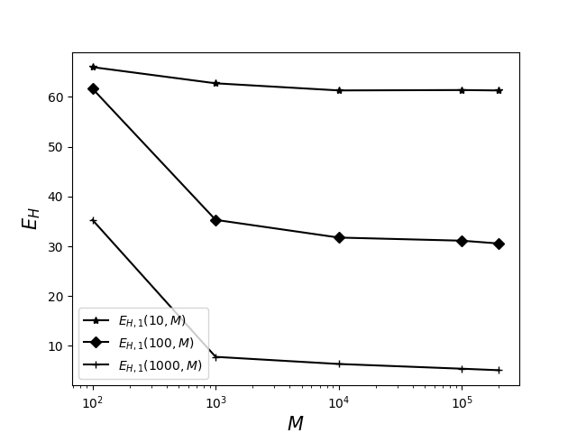
To first test the theorem-based methodology, we consider the Lorenz63 system. We integrate Lorenz system using the Runge-Kutta 4th order scheme with . As already mentioned in [17], this system is ergodic and has finite invariant measure. Hence the autocovariance always exist and can be identified with a subspace of and coincides with the classical Koopman operator on . Due to its weakly mixing nature, the only Koopman eigenfunction of Lorenz 63 is the constant function which has frequency 0. Let , where is the first component of Lorenz system and is the temporal mean of . We use to denote the leading renormalized singular value . Then the decomposition can be reduced to . As expected, Fig.1 does not display the tendency that converge to some nonzero value as .
V.2 A simple 4-dimensional system
Following one of the numerical examples in [17], we next consider a coupled system , which consists of the discrete-time Lorenz system and a rotation on the unit circle , i.e. , and . It is outlined in [17] that is an invariant measure. Still, the Lorenz system does not have non-trivial Koopman eigenfrequency and is ergodic. Therefore the autocovariance exists and coincides with the classical Koopman operator..
We choose the rotation to have period and define the observable
| (56) |
For simplicity, we also use to denote . Then as in Eq.(18).
Anticipated by our main theorem, the renormalized singular value of the trajectory matrix should then converge to the same quantity as the one calculated by Eq.(55). Hence it is worth to make a numerical comparison about obtained from Yosida’s formula and that from the singular values of .
The integration time step for Lorenz system is . The Runge-Kutta 4th order scheme is applied for integrating Lorenz system. The frequency we investigate is exactly the inverse of the period of , i.e. for Eq.(55). We use to denote the value of computed by Eq.(55), and to denote the value of which is computed from the singular value decomposition of . Note that are all integers which refer to the number of time steps instead of the exact time.
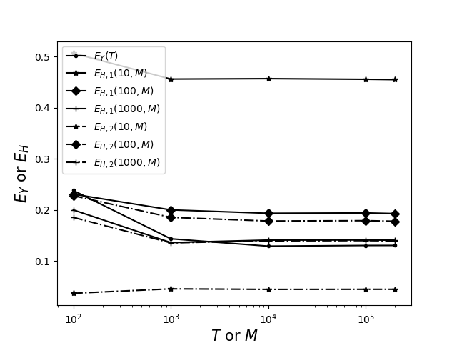
Fig.2 shows the numerical results of and . The value does not converge to , showing that is indeed a Koopman eigen frequency. We also computed . , meaning that the fraction of energy in represented by the Koopman eigenvector is about . Note that is close to , meaning that the leading singular value of the trajectory matrix indeed corresponds to the eigenfrequency . and seem to converge to the same value. This is because the Koopman eigenfrequencies always exist in pair, i.e. . Since the observable is real, the coefficient . Therefore, the total fraction of energy in that is represented by signals of period is about .
V.3 AVISO (DUACS) interpolated ocean topography data (1993-2019)
For final illustration, we consider sea surface height (SSH) estimates. The AVISO gridded products provide the global SSH interpolation since 1993, the year after the launch of the first satellite altimeter TOPEX/Poseidon. The SSH is interpolated daily at a grid resolution of . In this subsection, we use the main theorem to possibly assess the use of Koopman analysis for this dataset.
The assumption of the main theorem is the existence of autocovariance, which implies that the system should be stationary. We thus process the data by removing the overall constant rising tendency of SSH at each grid point over the decades (see for instance Fig.2 in [30]). We can not assert that the whole Earth system is ergodic and has an invariant measure, which includes the Earth, the atmosphere, ocean, all celestial bodies, but also the biology and living animals, etc. Hence we can not claim that the quantities , , etc. are associated to the classical Koopman operator. But, as we already stated, all these quantities are well-defined mathematically as long as the autocovariances exist. Moreover, in order to apply Yosida’s formula, we assume that the eigenvectors can be represented as a time series of the form for some . In this case, the output of Yosida’s formula must be . We renormalize the SSH at each grid point, to simply ensure the data to have zero mean and unit variance at every grid point. We first apply Yosida’s formula (Eq.55) to the global data to compute at every grid point, where . This quantity is computed for January 1, 1998, i.e. refers to the SSH at Jan. 1, 1998. Note that in theory, i.e. assuming the autocovariance exists and the data set large enough, this quantity does not depend on time. Since the data now has unit variance, can be interpreted as the fraction of energy in the SSH that is represented by the eigenfrequency . Similarly, since the SSH are real numbers, and represents the fraction of energy represented by the yearly signal.
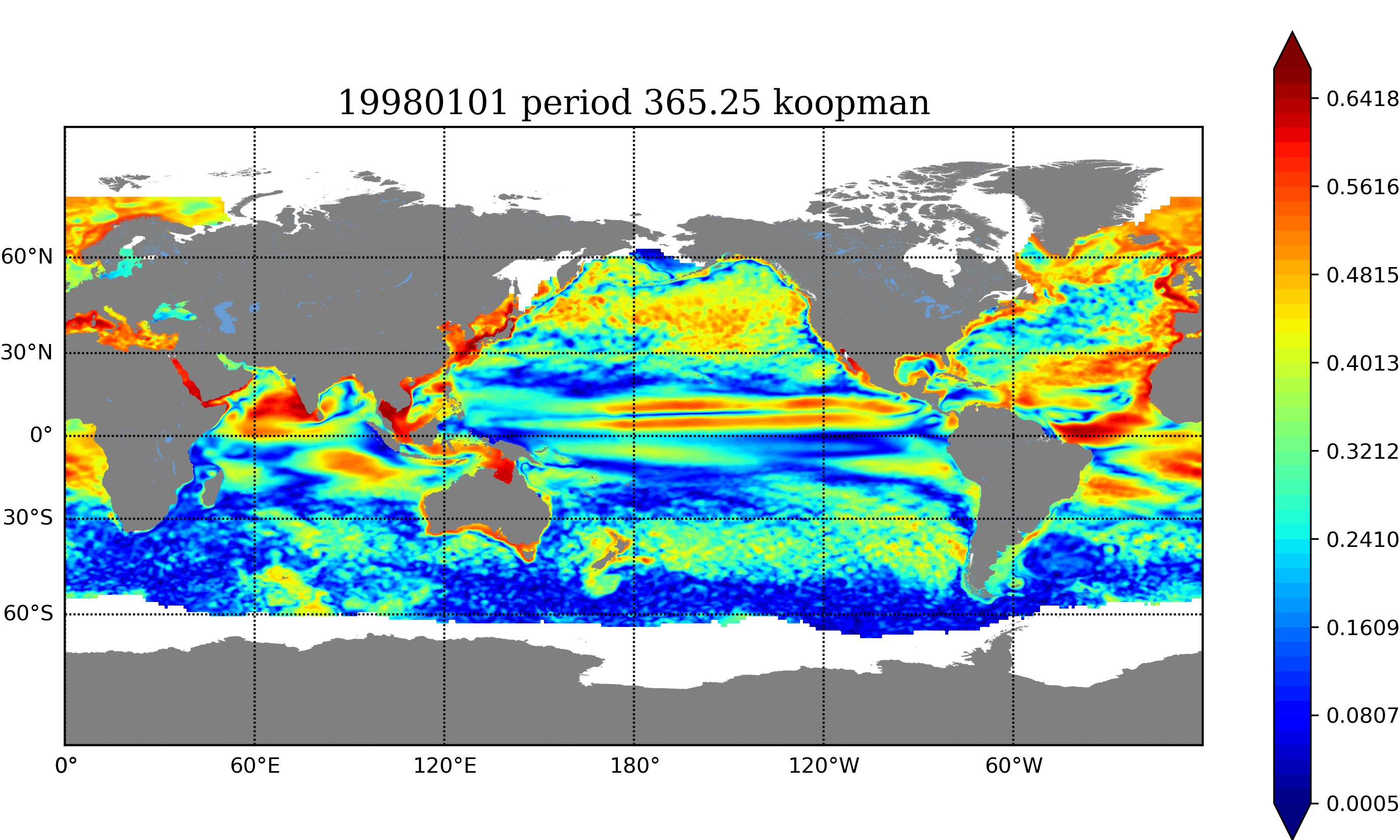
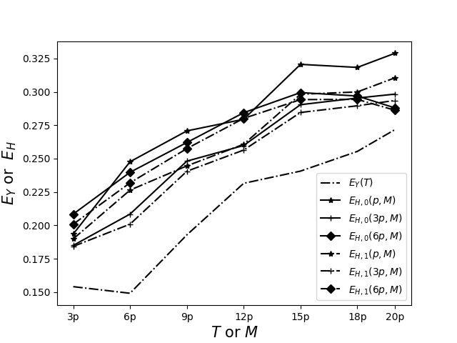
Fig.3 shows that more than of energy at the pacific ocean to the north of the equator (for instance at (W, N)) is represented by the yearly signal. Constructing the trajectory matrix for SSH at (W, N)), i.e. we choose W,N, we can then compare and , for , , , with year (days). Fig.4 shows that the first two renormalized singular values apparently converge to the fraction of energy represented by eigenfrequencies and . However, the third and fourth renormalized singular values do now show a sign of convergence. As shown in Fig.5, this is likely due to the overall limited length of the present-day data set regarding the high dimensional state space of the dynamical system at stake.

VI Conclusion
The main objective of this study is to provide a rigorous and practical method to identify Koopman eigenfrequencies for discrete-time ergodic and (finite) measure preserving dynamical systems. In the more general situation where we only assume that the time series has well-defined autocovariances, we define the Hilbert space purely based on the time series and the time shift operator that acts on . When the system is ergodic and has finite invariant measure, can be identified with the closure of the Krylov subspace generated by an observable , and the time-shift operator coincides with the classical Koopman operator on the observable space . This work follows the result in [7], but further extend the applicability of the Hankel-DMD. It provides a theorem-based practical way to help assess the results of the decomposition in terms of Koopman eigenfrequencies. It shows that the leading temporal EoFs, which are calculated from the eigen decomposition of the Gramian matrix, are indeed due to intrinsic eigenfrequencies. The main theorem provides partial theoretical foundation to several existing empirical methods including SSA,DAHD, and HAVOK. The main result shows that the discrete spectrum of can be characterized by the singular values (eigenvalues) of trajectory (Gramian, respectively) matrix. It remains to study whether the continuous spectrum can also be characterized by these matrices.
The numerical illustrations demonstrate the applicability of the theorem-based methodology for low dimensional systems. Yet, using sea surface height observables to inform about a very large dimension dynamical planet system, it is also apparent that one major difficulty of applying the main theorem might be the length of the data-set. An heuristic solution is to possibly associate the observables at different grid points, and/or to consider multiple observables, i.e. sea surface temperature. We reserve these investigations for future studies.
Acknowledgement
The authors acknowledge the support of the ERC EU project 856408-STUOD, the support of the ANR Melody project, the support from China Scholarship Council, and the support from the National Natural Science Foundation of China (Grant No. 42030406).
Appendix A An alternative proof of the weakly mixing property
In this appendix we provide an alternative proof of the weakly mixing property. Note that the proof of mixing theorem on page 39 of [27] implies that the weakly mixing property is equivalent to
| (57) |
for any continuous measure , which apparently is equivalent to
| (58) |
for any and continuous measure . We shall provide an alternative proof for proposition 5 and then derive Eq.(58) from proposition 5. To do this, we need the following lemma.
Lemma 6.
Let be a continuous finite measure on , and a sequence of subsets of such that for some fixed and for any . Then for any , there exists , and a subsequence , such that for any and .
Proof of lemma 6.
The idea of the proof is that we first show that there exists a point and such that and for any . Then we choose a small neighborhood of so that . This can be done merely because is a continuous measure. Let for , we have . Then we apply the same analysis to to find , etc. After doing the same analysis for times, we get and such that and for any and .
To prove that there exists a point and such that and for any . We prove by contradiction. Suppose that this is not true, i.e. for any there exists such that for any . Let . Then and . It means that as . This is apparently not true because . ∎
An alternative proof of proposition 5.
We prove by contradiction. We assume that proposition 5 does not hold. Then there exists and a sequence of , such that and
| (59) |
where . Note that for any . Let
| (60) |
Then .
Corollary 3.
Let be a continuous finite measure on . Then for any ,
| (62) |
Proof.
For any , let . For any , pick so that . Let . Then and
Then proposition 5 implies that
| (63) |
Hence
| (64) |
∎
Appendix B Proof of proposition 1
Proposition 1: Assume that the curve is continuous in . Let be an eigenfrequency of the discrete-time operator , i.e. there exists a time-series so that . Then there exists at least an integer , and , so that
| (65) |
for all .
Proof of proposition 1.
Consider where . Since , . It is easy to show that for any . So we have a closed loop in :
| (66) |
Now we do Fourier decomposition to this circle, i.e. for every integer , we define
| (67) |
Parseval’s theorem implies that
| (68) |
Therefore there exists an integer , such that . Now for any ,
| (69) |
In other words, is an eigen-vector of the continuous-time operator for any . ∎
References
- Schmid [2010] P. Schmid, Journal of Fluid Mechanics 656, 5 (2010).
- Rowley et al. [2009] C. Rowley, I. Mezic̈, S. Bagheri, P. Schlatter, and D. Henningson, Journal of Fluid Mechanics 641, 115 (2009).
- Saad [1980] Y. Saad, Linear Algebra and its Applications 34, 269 (1980).
- Chen et al. [2012] K. K. Chen, J. Tu, and C. Rowley, Journal of Nonlinear Science 22, 887 (2012).
- Wynn et al. [2013] A. Wynn, D. S. Pearson, B. Ganapathisubramani, and P. J. Goulart, Journal of Fluid Mechanics 733, 473–503 (2013).
- Tu et al. [2014] J. Tu, C. Rowley, D. M. Luchtenburg, S. Brunton, and J. Kutz, ACM Journal of Computer Documentation 1, 391 (2014).
- Arbabi and Mezic̈ [2017] H. Arbabi and I. Mezic̈, SIAM J. Appl. Dyn. Syst. 16, 2096 (2017).
- Kusaba et al. [2020] A. Kusaba, T. Kuboyama, and S. Inagaki, Plasma and Fusion Research 15, 1301001 (2020).
- Kutz et al. [2015] J. Kutz, X. Fu, and S. Brunton, arXiv: Dynamical Systems (2015).
- Williams et al. [2015a] M. Williams, I. Kevrekidis, and C. Rowley, Journal of Nonlinear Science 25, 1307 (2015a).
- Proctor et al. [2016] J. Proctor, S. Brunton, and J. Kutz, SIAM J. Appl. Dyn. Syst. 15, 142 (2016).
- Hemati et al. [2017] M. Hemati, C. Rowley, E. A. Deem, and L. Cattafesta, Theoretical and Computational Fluid Dynamics 31, 349 (2017).
- Taylor-King et al. [2020] J. P. Taylor-King, A. N. Riseth, W. Macnair, and M. Claassen, PLoS Computational Biology 16 (2020).
- Korda and Mezic̈ [2018] M. Korda and I. Mezic̈, Journal of Nonlinear Science 28, 687 (2018).
- Korda et al. [2020] M. Korda, M. Putinar, and I. Mezić, Applied and Computational Harmonic Analysis 48, 599 (2020).
- Williams et al. [2015b] M. O. Williams, C. W. Rowley, and I. G. Kevrekidis, Journal of Computational Dynamics 2, 247 (2015b).
- Das and Giannakis [2017] S. Das and D. Giannakis, Journal of Statistical Physics 175, 1107 (2017).
- Das and Giannakis [2018] S. Das and D. Giannakis, arXiv: Dynamical Systems (2018).
- Giannakis et al. [2018] D. Giannakis, S. Das, and J. Slawinska, arXiv: Dynamical Systems (2018).
- Giannakis [2020] D. Giannakis, Research in the Mathematical Sciences 8, 1 (2020).
- Nuske et al. [2021] F. Nuske, S. Peitz, F. Philipp, M. Schaller, and K. Worthmann, arXiv (2021).
- Ghil et al. [2002] M. Ghil, M. R. Allen, M. D. Dettinger, K. Ide, D. Kondrashov, M. E. Mann, A. Robertson, A. Saunders, Y. Tian, F. Varadi, and P. Yiou, Reviews of Geophysics 40, 3 (2002).
- Kondrashov et al. [2020] D. Kondrashov, E. Ryzhov, and P. Berloff, Chaos 30 6, 061105 (2020).
- Brunton et al. [2017] S. L. Brunton, B. W. Brunton, J. L. Proctor, E. Kaiser, and J. N. Kutz, Nature Communications 8 (2017).
- Yosida [1995] K. Yosida, Functional Analysis (Springer, Berlin, Heidelberg, 1995).
- Borthwick [2020] D. Borthwick, Spectral Theory: Basic Concepts and Applications, 1st ed., Graduate Texts in Mathematics №284 (Springer International Publishing;Springer, 2020).
- Halmos [1956] P. R. Halmos, Lectures on Ergodic Theory (Chelsea Publishing Company, New York, N.Y, 1956).
- Mezić and Banaszuk [2004] I. Mezić and A. Banaszuk, Physica D: Nonlinear Phenomena 197, 101 (2004).
- Mezić [2005] I. Mezić, Nonlinear Dynamics 41, 309 (2005).
- Cazenave and Llovel [2010] A. Cazenave and W. Llovel, Annual review of marine science 2, 145 (2010).