Optimal metrology with programmable quantum sensors

Abstract

Quantum sensors are an established technology that has created new opportunities for precision sensing across the breadth of science. Using entanglement for quantum-enhancement will allow us to construct the next generation of sensors that can approach the fundamental limits of precision allowed by quantum physics. However, determining how state-of-the-art sensing platforms may be used to converge to these ultimate limits is an outstanding challenge. In this work we merge concepts from the field of quantum information processing with metrology, and successfully implement experimentally a programmable quantum sensor operating close to the fundamental limits imposed by the laws of quantum mechanics. We achieve this by using low-depth, parametrized quantum circuits implementing optimal input states and measurement operators for a sensing task on a trapped ion experiment. With 26 ions, we approach the fundamental sensing limit up to a factor of 1.45(1), outperforming conventional spin-squeezing with a factor of 1.87(3). Our approach reduces the number of averages to reach a given Allan deviation by a factor of 1.59(6) compared to traditional methods not employing entanglement-enabled protocols. We further perform on-device quantum-classical feedback optimization to ‘self-calibrate’ the programmable quantum sensor with comparable performance. This ability illustrates that this next generation of quantum sensor can be employed without prior knowledge of the device or its noise environment.

I Introduction

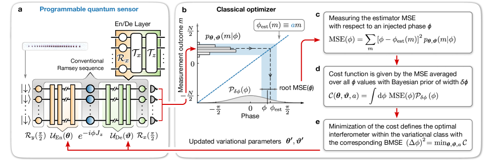
Figure 1: Measurement and feedback concept for variational quantum Ramsey interferometry circuits. a A programmable quantum sensor executes a generalized Ramsey sequence with entangling and decoding unitaries $\mathcal{U}_{\text{En}}$, and $\mathcal{U}_{\text{De}}$ on $N$ particles. The unitaries are made from a repeating sequence of sensor resource gates, here collective qubit rotations $\mathcal{R}_{x,y,z}$, and infinite-range one axis twistings $\mathcal{T}_{x,y,z}$ with parameter sets $\left\{\bm{\theta},\bm{\vartheta}\right\}$. b Measurement of the collective spin $z$-projection results in a difference $m$ of particles in $\ket{\uparrow}$ and $\ket{\downarrow}$ states. This is used to produce an estimate of the phase $\phi$ using a linear phase estimator $\phi_{\text{est}}$ with slope $a$. Prior knowledge of $\phi$ is encoded via the distribution $\mathcal{P}_{\delta\phi}$ taken here as Gaussian with variance $(\delta\phi)^{2}$ and zero mean. c The conditional probability $p_{\bm{\theta},\bm{\vartheta}}(m|\phi)=\big{|}\bra{m}\mathcal{R}_{x}(\tfrac{\pi}{2})\,\mathcal{U}_{\rm De}(\boldsymbol{\vartheta})\,e^{-i\phi J_{z}}\,\mathcal{U}_{\rm En}(\boldsymbol{\theta})\mathcal{R}_{y}(\tfrac{\pi}{2})\ket{\downarrow}^{\otimes N}\big{|}^{2}$ can be evaluated numerically or sampled in the experiment to calculate a mean squared error with respect to the true phase and the used estimator. d An operational cost function $\mathcal{C}$ can be defined to quantify the interferometer performance for a variational sequence parameter set $\left\{\bm{\theta},\bm{\vartheta}\right\}$. e Minimization of the cost function is achieved by determining new parameter sets $\left\{\bm{\theta^{\prime}},\bm{\vartheta^{\prime}}\right\}$ and comparing the associated costs either on-device or using classical simulation.

Quantum sensing, that is using quantum systems to enable or enhance sensing, is arguably the most mature quantum technology to date. Quantum sensors have already found applications in many disciplines. The majority of these sensors are ‘quantum-enabled’; using the properties of a quantum system to perform a metrological task. Such applications have expanded rapidly including biology [1, 2], medicine [3], chemistry [4], or precision navigation [5] alongside traditional applications in physics such as inertial sensing [6, 7, 8] or timekeeping [9]. Quantum-enabled sensors perform close to or at the standard quantum limit (SQL) which originates from the quantum noise of the classical states used to initialise them. The latest generation of sensing technologies is going beyond the SQL by employing entangled states. These ‘quantum-enhanced’ sensors are used in gravitational wave astronomy [10], allow crossing the long-standing photodamage limit in life science microscopy [11], and promise improved atomic clocks [12]. However, these existing quantum-enhanced sensors, while beating the SQL, do not come close to what is ultimately allowed by quantum mechanics [13]. Convergence to this ultimate bound is an open challenge in sensing [14].

A parallel development in quantum technology that has seen massive progress alongside quantum sensing is quantum information processing, pursuing a ‘quantum advantage’ in computation and simulation on near-term hardware [15]. A crucial capability that has been developed in this context is the targeted creation of entangled many-body states [16, 17, 18, 19, 20]. A promising strategy there is to employ low-depth variational quantum circuits through hybrid quantum-classical algorithms [21, 22, 23, 24]. Integrating this ability to program tailored entanglement into all aspects of sensing — including measurement protocols [25, 26] — will allow the construction of the next generation of sensors, able to closely approach fundamental sensing limits. The concept of such a ‘programmable quantum sensor’ can be implemented on a great variety of hardware platforms, and is applicable to a wide range of sensing tasks. Moreover, their programmability makes such sensors amenable to on-device variational optimization of their performance, enabling an optimal usage of entanglement even on noisy and non-universal present-day quantum hardware.

Here we demonstrate the first experimental implementation of a programmable quantum sensor [27] performing close to optimal with respect to the absolute quantum limit in sensing. We consider optimal quantum interferometery on trapped ions as a specific but highly pertinent example that promises applications ranging from improving atomic clocks and the global positioning system to magnetometry and inertial sensing. Our general approach is to define a cost function for the sensing task relative to which optimality is defined. We employ low-depth variational quantum circuits to search for and obtain optimal input states and measurement operators on the programmable sensor. This allows us to apply on-device quantum-classical feedback optimization, or automatic ‘self-calibration’ of the device, achieving a performance close to the fundamental optimum.

Optimal quantum interferometry

Our study below aims at optimal Ramsey interferometry to estimate a phase $\phi$ (Fig. 1 a). In this context we aim to identify a suitable metrological cost function to quantify optimality. An established metric here is the mean squared error $\mathrm{MSE}(\phi)$ whose minimization yields the best average signal-to-noise ratio for phase estimation at fixed signal. Traditionally, the optimization is done locally, i.e. for a small neighbourhood of phases around an a priori-specified value. This is achieved in the Fisher information approach, which underlies the discussion of Ramsey interferometry with squeezed spin states (SSS) [28] and, in particular, GHZ states [29]. Within this local approach the GHZ states are shown to saturate the so-called Heisenberg limit (HL) [30].

In contrast, we are interested in an optimization for a finite phase range $\delta\phi$, given by the desired dynamic range of the interferometer [13, 31]. This choice is motivated by applications using single-shot measurements such as in atomic clocks [32, 14]. We highlight that in frequency estimation applications the phase $\phi$ acquired during interrogation is not restricted to the $[-\pi,\pi)$ interval. Therefore the effect of the phase slipping outside this interval has to be taken into account as it leads to a permanent error in the frequency estimation. [32, 33, 14]. Under these circumstances the optimization may be accomplished in a Bayesian approach to optimal interferometry [33], where a prior distribution of the phase, $P_{\delta\phi}(\phi)$ with width $\delta\phi$ defined as the standard deviation, is updated by the measurement to a posterior distribution with smaller width $\Delta\phi$. Consequently, we find as the metrological cost function $\mathcal{C}$ the Bayesian MSE (BMSE), $\mathcal{C}\equiv\int{\mathrm{d}\phi\,\textrm{MSE}(\phi)\mathcal{P}_{\delta\phi}(\phi)}$ (see Fig. 1 b - e), that is the posterior mean squared error characterizing the phase probability distribution given the measurement outcome $m$, and whose minimum we identify here with $(\Delta\phi)^{2}$. The optimal quantum interferometer (OQI) is thus obtained by minimization of the cost $\mathcal{C}$, that is the BMSE, over all entangled input states $\ket{\psi_{\mathrm{in}}}$, general measurements $\mathcal{M}$, and estimator functions $\phi_{\mathrm{est}}(m)$ [33]. We emphasize that the OQI with large $\delta\phi$ will differ greatly from SSS or GHZ state-based interferometers, which optimize for local phase sensitivity $\delta\phi\rightarrow 0$ [33, 14].

Our goal below is to closely approach the OQI on programmable quantum sensors. We pursue a variational approach to optimal quantum metrology [14], using a limited set of quantum operations available on a specific sensor platform. We consider a generalized Ramsey interferometer with an entangling operation $\mathcal{U}_{\mathrm{En}}$ preparing an entangled state $\ket{\psi_{\mathrm{in}}}$ from the initial product state $\ket{\downarrow}^{\otimes N}$ of $N$ particles, and a decoding operation $\mathcal{U}_{\mathrm{De}}$ transforming a typical observable, e.g. $z$-projection of collective spin, into a general measurement (Fig. 1 a and M1). The variational approach consists of an ansatz, where both $\mathcal{U}_{\mathrm{En}}$ and $\mathcal{U}_{\mathrm{De}}$ are approximated by low-depth quantum circuits. These are built from ‘layers’ of basic resource gates, which are given here by collective Rabi oscillations (qubit rotations) and collective entangling operations, commonly called infinite-range one axis twisting (OAT) interactions [34] (see M2 Eqs. 9) due to their action on the Bloch sphere. These resources are available in many atomic or trapped ion systems [12, 35]. A quantum sensor is then programmed by specifying variational quantum circuits through $\mathcal{U}_{\mathrm{En}}(\bm{\theta})$ and $\mathcal{U}_{\mathrm{De}}(\bm{\vartheta})$, consisting of $n_{\text{En}}$ and $n_{\text{De}}$ ‘layers’, respectively. These circuits define the conditional probability $p_{\bm{\theta},\bm{\vartheta}}(m|\phi)$, which describes the statistics of measurement outcomes $m$ given an input phase $\phi$. Together with a choice of phase estimator $\phi_{\mathrm{est}}(m)$ it determines the MSE, and in turn together with the prior $\mathcal{P}_{\delta\phi}$ the cost function $\mathcal{C}$. By varying the parameter vectors $\bm{\theta}$ and $\bm{\vartheta}$ we can therefore optimize the programmable quantum sensor for a given sensor platform and task. We refer to Methods M1 for a technical summary and to Ref. [14] for details and intuitive explanation of the method (see II. C).

We implement the optimal Ramsey interferometry above on a compact trapped-ion quantum computing platform [17]. This platform is used as a programmable quantum sensor, where in this work a linear chain of up to 26 ⁴⁰Ca⁺ ions is hosted in a Paul trap. Optical qubits are encoded in the ground state $\ket{\textrm{4\,S}_{1/2},m_{J}=-1/2}$ and excited state $\ket{\textrm{3\,D}_{1/2},m_{J}=-1/2}$, which are connected via an electric quadrupole clock transition near $729\text{\,}\mathrm{nm}$. Technical details of the implementation can be found in the Supplementary Material, in particular state preparation and readout (S1), implementation and calibration of unitaries via the Mølmer-Sørensen interaction (S2), and technical restrictions imposed on the scheme (S3).

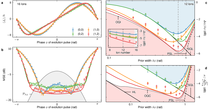
Figure 2: Generalized Ramsey sequence performance measurements. Markers are experimental data with 1$\sigma$ statistical uncertainties, and solid lines are theory with no free parameters. a 16 ion chain expectation value of spin operator $\left<J_{z}\right>/\hbar$ as a function of evaluation pulse phase $\phi$. 50 experiments are averaged per point, and 5 full traces are recorded to calculate mean and standard deviation of each curve. b MSE calculated from traces in a for optimal linear estimator $\phi_{\text{est}}$. Overlaid in grey is the prior distribution $\mathcal{P}_{\delta\phi}\left(\phi\right)$ with $\delta\phi\approx 0.79$ (minimum of BMSE vs $\delta\phi$). c $\Delta\phi/\delta\phi$ as a function of prior width $\delta\phi$ for 12 ions in the four variational sequences. The blue shaded region corresponds roughly to classical Ramsey sequences. The red shaded region is inaccessible to single-shot measurement schemes, where the boundary corresponds to the optimal quantum interferometer (OQI) [33]. Each point is produced by numerically integrating curves as in b over $\phi$ as per Eq. 2. The OQI, the standard quantum limit (SQL) and the phase slip limit (PSL) are indicated by black lines (Methods M4). Inset $\Delta\phi/\delta\phi$ as a function of particle number at the prior width indicated by the dashed line. $N=16$ points calculated from data in b. d Allan deviation normalized to noise bandwidth $b_{\alpha}$, averaging time $\tau$ and reference frequency $\omega_{A}$ as a function of prior width with PSL, SQL, Heisenberg limit (HL) and optimal quantum clock (OQC) based on the OQI are indicated by black lines (Methods M5). Raw data, color scheme, and markers from c.

II Results

We study the performance of the variationally optimized Ramsey sequences for four different choices of entangling and decoding layer depths $(n_{\text{En}},n_{\text{De}})$ generating four distinct circuits: $(0,0)$ being a classical coherent spin state (CSS) interferometer [30] as the baseline comparison. All other sequences have been variationally optimized, $(1,0)$ being similar to a squeezed spin state (SSS) interferometer [30], $(0,2)$ with a CSS input state and tailored measurement, and finally $(1,2)$ with both tailored input and measurement.

Direct implementation of theory parameters

Following the execution of a Ramsey sequence (Eq. 1 in M1, or S2) we perform projective measurements at different Ramsey phases $\phi$ to reconstruct the expectation value of the total spin $z$ projection, $J_{z}$ (Fig. 2 a). From the measurements we construct the MSE (Fig. 2 b) using the linear estimator function $\phi_{\text{est}}=am$ with slope $a$ which minimizes the cost function $\mathcal{C}$ obtained from integration according to Eq. 4 (see S4 and SI Tab. 1 for calculation, and S9 for discussion of other estimators). Qualitatively, Ramsey sequences with input state squeezing ($n_{\text{En}}>0$) dip below the CSS around $\phi=0$ as seen in Fig. 2 b. This dip is a manifestation of reduced projection noise. Sequences with optimized measurement operators ($n_{\text{De}}>0$) exhibit a broader range of $\phi$ values for which the MSE is comparable to the $\phi=0$ value. This is a consequence of the enhanced dynamic range that the non-trivial decoding unitaries impart, that is, the range over which the expectation value $\left<J_{z}\right>/\hbar$ remains well-approximated by the linear estimator (Fig. 2 a). Combining tailored input and measurements ($n_{\text{En}},n_{\text{De}}>0$) yields an MSE which is both lower and wider than the CSS baseline.

To study this behaviour quantitatively as a function of the prior width $\delta\phi$ and particle number $N$ we calculate the BMSE scaled to the prior width $\delta\phi$ used. This is a convenient measure since $\delta\phi$ encapsulates prior knowledge of $\phi$ and $\Delta\phi$ encapsulates posterior knowledge after measurement. Their ratio $\Delta\phi/\delta\phi$ is therefore bounded on the interval $[0,1]$. We investigate this quantity for $\delta\phi\in\left[0.2,1\right]\text{rad}$ as a representative sample of the parameter space, since no information is gained as $\delta\phi\rightarrow 0$, due to quantum projection noise overwhelming the signal, or $\delta\phi\rightarrow\pi$, due to phase slips outside the interval of unambiguous phase estimation (Fig. 2 c). For more details see Methods M4.

All variationally optimized sequences outperform the CSS within this measure (Fig. 2 c). The effect of change in dynamic range is evident in the location of a sequence’s minimum. Minima of sequences with decoding layers shift towards larger prior widths with respect to the CSS, while for the direct spin-squeezing $(1,0)$ it shifts towards smaller values. Sequences with a larger number of operations deviate more strongly from the theory predictions due to accumulation of gate errors. This behaviour is consistent across a range of particle numbers (Fig. 2 c inset). The deviation decreases as the system size does. We attribute this to the decrease in the fidelity of entangling operations [17].

The $(1,2)$ scheme outperforms all others despite the increased complexity. In particular, it outperforms the simple spin-squeezing $(1,0)$ scheme at both the optimal $\delta\phi$ for $(1,2)$ and $(1,0)$ approaching closely the OQI (see Tab. 1). Specifically, for 26 particles and at their respective optimal prior widths, the $(1,0)$ sequence approaches the OQI up to a factor of 1.87(3) (or $2.73(7)\text{\,}\mathrm{dB}$), and the $(1,2)$ sequence up to a factor of 1.45(1) (or $1.61(2)\text{\,}\mathrm{dB}$). At this optimal prior width the $(1,2)$ sequence would reduce the required number of averages to achieve the same Allan deviation as a classical Ramsey sequence by a factor of 1.59(6). A pictorial interpretation, in terms of Wigner distribution, of the optimized (optimal) interferometer can be found in Ref. [14].

	$N=12$		$N=26$
$\delta\phi$	0.6893	0.792	0.5480	0.7403
$(0,0)$	$-3.56(3)\text{\,}\mathrm{dB}$	$-3.63(8)\text{\,}\mathrm{dB}$	$-3.22(3)\text{\,}\mathrm{dB}$	$-4.53(3)\text{\,}\mathrm{dB}$
$(1,0)$	$-4.61(12)\text{\,}\mathrm{dB}$	$-4.34(4)\text{\,}\mathrm{dB}$	$-5.63(7)\text{\,}\mathrm{dB}$	$-5.39(2)\text{\,}\mathrm{dB}$
$(1,2)$	$-5.06(11)\text{\,}\mathrm{dB}$	$-5.18(8)\text{\,}\mathrm{dB}$	$-5.84(9)\text{\,}\mathrm{dB}$	$-6.75(2)\text{\,}\mathrm{dB}$
OQI	$-5.86\text{\,}\mathrm{dB}$		$-8.36\text{\,}\mathrm{dB}$

Table 1: Comparison of measured values of $\Delta\phi/\delta\phi$ at two values of $\delta\phi$ corresponding to the minima of the $(1,0)$ (smaller $\delta\phi$) and $(1,2)$ (larger $\delta\phi$) scheme, respectively. Note that the location of the minimum for $(1,2)$ and $(0,0)$ is identical to within the measurement resolution presented. For reference, the minimum of the optimal quantum interferometer (OQI, border to shaded red region in Fig. 2 c) is given as well.

For atomic clock settings $\Delta\phi$ can be rescaled to calculate the Allan deviation of a deadtime-free clock (see M5), as shown in Fig. 2 d given the same raw data.

On-device quantum-classical feedback optimization

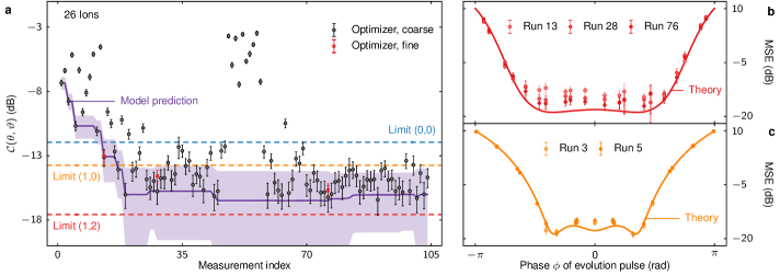
Figure 3: On-device hybrid quantum-classical optimization performance with 26 ions at $\delta\phi\approx 0.74$ (minimum BMSE vs $\delta\phi$), all error bars are 1$\sigma$ statistical uncertainties. a Optimizer cost function $\mathcal{C}$ as a function of measurement index (runs). Estimate is based on integration using 10 Hermite-Gauss nodes (S4) and 100 repetitions per point. Dashed lines indicate the achievable performance with the indicated sequences. Red crosses correspond to the automated fine scans displayed in panel b. b Automated fine scans (S) of the MSE with 20 nodes and 250 repetitions for three measurement indices. c Analogous fine scans from optimizer run using $(1,0)$ sequence. Estimates based on 21 nodes and 250 repetitions per point.

We further investigate the parameter ‘self-calibration’ of the scheme in a regime where manual calibration is challenging, such that we expect direct application of theoretically optimal angles to no longer perform well. In particular, this is a regime where accurately calibrating the twisting parameters in $(\bm{\theta},\bm{\vartheta})$ is no longer feasible. Minimization of the cost function is therefore achieved by a feedback loop where a classical optimization routine proposes new parameter sets to trial based on measurements performed on the quantum sensor. We employ a global, gradient-free optimization routine with an internal representation or ‘meta-model’ of the cost function (S5).

The meta-model uses the known structure of the resource operations to learn an estimate of the cost function landscape based on the measurements, as seen in Fig. 3 a for a 26 ion chain and the $(1,2)$ circuit. Calibration of twisting angles is performed at a lower ion number (20), and then approximately scaled to the larger number. The cost function estimates are below the competing CSS $(0,0)$ and direct spin-squeezing $(1,0)$ after $\approx 20$ measurements despite this lack in accurate calibration. A full iteration of the algorithm is completed after $\approx 50$ measurements in Fig. 3 a.

Measurement points that the algorithm deems promising candidates for a minimum are resampled using ‘fine’ scans (S6). Fine scans serve to increase the algorithm’s confidence about predictions made on sparse data by better sampling, and relaxing symmetry assumptions of ‘coarse’ scans. Fine scans show convergence towards the theory optimum as the algorithm progresses (Fig. 3 b). Convergence is achieved more rapidly for the $(1,0)$ sequence (Fig. 3 c) due to the lower number of variational parameters, and consequently smaller parameter space. This convergence in both sequences despite the inability to accurately calibrate is a manifestation of the optimizer’s ability to learn and correct for correlated gate (calibration) errors.

Frequency estimation

All measurements up to this stage were taken by driving rotations $\mathcal{R}_{y}(\phi)$ with resonant laser pulses as a consequence of our technical implementation (S2). This allows for deterministic mapping of the $\phi$ space, but in atomic clock experiments the phase $\phi$ would instead be imparted by the residual detuning of the drive from the atomic reference under the influence of noise. To gauge the performance of a clock we perform frequency estimation experiments. We calculate the variance of the frequency estimator from the known injected noise for a standard CSS interferometer, and the $(1,2)$ interferometer optimized for a prior width $\delta\phi\approx 0.69$ (S7).

The optimized sequence outperforms the CSS for all considered Ramsey times (Fig. 4). In particular, this demonstrates robustness of the scheme with respect to variations in the prior width (Ramsey time, S8). The deviation between experiment and theory predictions can be explained by two observations. First, we independently measured predominantly frequency flicker noise of bandwidth $b_{\alpha}\approx 2\pi\cdot$6\text{\,}\mathrm{H}\mathrm{z}$$ (S7) on the laser which is not present in the simple simulation. Second, the MSE used in the simulation is the ideal, theoretically-achievable one, while the experiment has deviations from the theory such as in Fig. 2 b. Simulating the metrology experiments with these additional noise sources restores good match between data and prediction. We note that this problem is not apparent in the BMSE or the Allan variance plots (Fig. 2 c and d) since it arises solely in the $\mathcal{R}_{z}$ operation we employ here, while $\phi$ was imparted via $\mathcal{R}_{y}$ there.

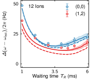
Figure 4: Frequency measurement using 12 ions with a standard and variationally optimized Ramsey sequence. Shown is the standard deviation of the difference between known injected and estimated frequency detuning. Markers are experimental data with uncertainty (finite sampling and projection noise). Dashed lines are theory simulations with no free parameters, while solid lines are simulation of measurement performance including a residual laser flicker noise of $b_{\alpha}\approx 2\pi\cdot$6\text{\,}\mathrm{H}\mathrm{z}$$, and shading indicates error margin of simulation.

III Discussion and outlook

Intermediate-scale quantum devices, acting as quantum sensors, provide the toolset to program entanglement and collective measurements to approach the ultimate limits of parameter estimation compatible with the laws of quantum physics. The present work has demonstrated programming a close-to-optimal quantum interferometer with (up to) $N=26$ entangled atoms on a trapped-ion quantum computer. A key element of our work has been to identify a pathway towards optimal quantum sensing by formulating it as a variational quantum algorithm, where circuits of increasing depths allow convergence towards the ultimate sensing limit. This limit is approached by optimizing the circuits using a task-specific cost function. The shallow quantum circuits used here are built from native, imperfect trapped-ion quantum operations, and are already shown to yield results close to optimal metrology. In a broader context, this suggests that the variational approach to optimal quantum sensing is both flexible and hardware efficient. When combined with the linearly-growing solution Hilbert space this indicates the potential to scale to significantly larger particle numbers.

Variational optimal metrology is immediately applicable to a wide range of sensing tasks. Our demonstration of generalized Ramsey interferometry is relevant for atomic clocks, and we discuss the projected gains in Allan deviation in the Supplementary Material (S10). Furthermore, the prevalence of Ramsey interferometry in metrology renders our approach relevant to the measurement of magnetic fields [36], inertia [37], displacement and electric fields [38], as well as force measurements [39]. While here we demonstrated quantum estimation of a single parameter, the present technique of variational optimal metrology readily generalizes to the multi-parameter case [40].

Our approach is furthermore immediately applicable to other sensing platforms. Variational quantum metrology can for example be implemented on programmable quantum simulators [27] with well-established capabilities, in particular in higher spatial dimensions. While these readily scale to large particle numbers, they provide only non-universal entanglement operations via finite-range interactions. The ‘on-device’ optimization of the metrological cost function, as demonstrated in the present work, then not only serves to find optimal input states and measurement protocols in presence of ‘real world’ device imperfections and noise. Instead, it then also addresses the underlying computationally hard problem of preparation and manipulation of many-body quantum states. For increasing particle numbers this provides an example of a quantum device operating in a regime of relevant quantum advantage, where many-body quantum states are both prepared and subsequently exploited in optimal metrology.

Methods

M1 Variational Ramsey interferometer

In variational Ramsey interferometry, the quantum sensor is initially prepared in the collective spin down state, and subsequently executes the variational Ramsey sequence given by

$$\mathcal{U}_{\text{R}}(\phi,\bm{\theta},\bm{\vartheta})=\mathcal{R}_{x}(\tfrac{\pi}{2})\mathcal{U}_{\text{De}}(\bm{\vartheta})\mathcal{R}_{z}(\phi)\mathcal{U}_{\text{En}}(\bm{\theta})\mathcal{R}_{y}(\tfrac{\pi}{2}),$$ (1)

where $\mathcal{R}_{x,y,z}$ are collective Rabi oscillations, and $\mathcal{U}_{\text{En}}(\bm{\theta}),\mathcal{U}_{\text{De}}(\bm{\vartheta})$ are entangling and decoding circuits, with control parameters $\bm{\theta},\bm{\vartheta}$ (see Methods M2). In between the two operations, the sensor interacts with an external field which imprints a phase $\phi$ onto the constituent particles. It is important to note that the Ramsey sequence is $2\pi$-periodic in $\phi$ and hence phases can only be distinguished modulo $2\pi$.

After executing $\mathcal{U}_{\text{R}}(\phi,\bm{\theta},\bm{\vartheta})$, we perform projective measurements of the collective spin yielding outcomes $m$ (difference of particles in $\ket{\uparrow}$ and $\ket{\downarrow}$). The phase $\phi$ is estimated from $m$ by means of a linear phase estimator $\phi_{\rm est}(m)=a\,m$, which is optimal for the variational interferometer [14] and near-optimal for CSS- and SSS interferometers at the particle numbers considered here [41]. We provide a quantitative comparison between the different estimation functions in S9.

The goal is to find parameters $\bm{\theta},\bm{\vartheta},a$, that give the best possible performance of the sensor. The performance of the sensor intended to correctly measure a given phase $\phi$ can be quantified by the mean squared error

$$\textrm{MSE}(\phi)=\sum_{m}{\left[\phi-\phi_{\rm est}(m)\right]^{2}p_{\bm{\theta},\bm{\vartheta}}(m|\phi)},$$ (2)

where

$$p_{\bm{\theta},\bm{\vartheta}}(m|\phi)=\big{|}\bra{m}\mathcal{U}_{\text{R}}(\phi,\bm{\theta},\bm{\vartheta})\ket{\downarrow}^{\otimes N}\big{|}^{2}$$ (3)

is the probability to observe a measurement outcome $m$, given $\phi$, and for given circuit parameters $\bm{\theta},\bm{\vartheta}$.

In Bayesian phase estimation we are interested in a sensor that performs well for a range of phases $\phi$, occurring according to a prior distribution $P_{\delta\phi}(\phi)$. We assume $P_{\delta\phi}(\phi)$ to be a normal distribution with variance $(\delta\phi)^{2}$ and zero mean throughout, which is a choice particularly relevant for applications like atomic clocks. Note that the normal distribution has a finite probability for phase slips outside the unambiguous phase interval, determined by the period of $\mathcal{U}_{\text{R}}$. Phase slips contribute to the MSE, and dominate for $\delta\phi\gtrsim 1$ (see M4).

A meaningful cost function for the sensor’s overall performance is the average MSE, weighted according to the prior phase distribution $P_{\delta\phi}$

$$\mathcal{C}(\bm{\theta},\bm{\vartheta},a)=\int{\text{d}\phi\ \textrm{MSE}(\phi,\bm{\theta},\bm{\vartheta})\mathcal{P}_{\delta\phi}\left(\phi\right)},$$ (4)

called Bayesian mean squared error (BMSE).

In this work, the parameters $(\bm{\theta},\bm{\vartheta},a)$ are optimized with respect to the cost function $\mathcal{C}$, either numerically (see Fig. 2), or on-device in a variational feedback loop (see Fig. 3). For on-device optimization, the parameter $a$ is held fixed at the numerically calculated optimal value.

To evaluate the cost function $\mathcal{C}$ in the variational feedback loop we run the Ramsey sequence, while exposing the sensor to a sequence of known injected phases $\phi_{i}$. The cost function value is then estimated as

$$\mathcal{C}(\bm{\theta},\bm{\vartheta},a)\simeq\sum_{i}\textrm{MSE}(\phi_{i})P_{\delta\phi}(\phi_{i})w_{i},$$ (5)

where $w_{i}$ are Hermite Gaussian integration weights (see S4).

The minimum of the cost function $(\Delta\phi)^{2}=\min_{\bm{\theta},\bm{\vartheta},a}\mathcal{C}$ can be interpreted [42] as

$$(\Delta\phi)^{2}\approx\sum_{m}(\Delta\phi_{m})^{2}p(m)$$ (6)

i.e. the variances$(\Delta\phi_{m})^{2}$ of the posterior distributions $p(\phi|m)$ averaged according to the probability $p(m)$ to observe the measurement outcome $m$. Therefore we refer to $\Delta\phi$ as the posterior width.

M2 Ramsey sequence

Following [14] the explicit form of the entangling and decoding unitaries are

$$\mathcal{U}_{\text{En}} =\prod_{k=1}^{n_{\text{En}}}\mathcal{R}_{x}(\theta_{k}^{3})\mathcal{T}_{x}(\theta_{k}^{2})\mathcal{T}_{z}(\theta_{k}^{1})$$ (7)

$$\mathcal{U}_{\text{De}} =\prod_{k=1}^{n_{\text{De}}}\mathcal{T}_{z}(\vartheta_{k}^{1})\mathcal{T}_{x}(\vartheta_{k}^{2})\mathcal{R}_{x}(\vartheta_{k}^{3}).$$ (8)

Here $\mathcal{R}_{x,y,z}$ are collective Rabi oscillations, and $\mathcal{T}_{x,y,z}$ are one-axis twisting (OAT) operations. Mathematically these operations can be represented as

$$\mathcal{R}_{x,y,z}(\beta)=\text{e}^{-i\beta J_{x,y,z}},\quad\mathcal{T}_{x,y,z}(\chi)=\text{e}^{-i\chi J_{x,y,z}^{2}}$$ (9)

where $\beta$ and $\chi$ are angles that depends on the interaction strength and time, and $J_{x,y,z}$ are collective spin operators in the Cartesian basis. We denote the collection of the three operations in Eqs. 7, 8 with the same subscript as one layer, and we denote by $n_{\text{En}}$ and $n_{\text{De}}$ the number of entangling and decoding layers.

M3 Effects of resource restrictions

The globally optimal variational parameter sets depend on the ion number via the prior width. However, we may additionally restrict them based on platform constraints of fundamental or practical nature to find sets optimal with respect to device capabilities. This adds to the adaptability inherent to the scheme: We tailor the cost function to the sensing task, and the sequence resources, while parameter ranges are constrained by the experimental hardware. Combined this assists with assessing and interpretation of attainable results given real-world constraints.

Furthermore, in systems of moderate size of order 50 and above this leads to the Allan deviation scaling down with particle number $N$ or Ramsey time $T_{R}$ at close to the ($\pi$-corrected) Heisenberg limit [13, 43] up to a logarithmic correction [14, 44]. This is of great practical utility in situations where measurements are made with a fixed budget in particle number or measurement time.

M4 Bounds on the Bayesian mean squared error

In the Bayesian framework, a bound on the BMSE in the limit of a narrow prior, $\delta\phi\ll 1$, is imposed by quantum measurement fluctuations as captured by van Trees’ inequality [45],

$$(\Delta\phi)^{2}\geq\frac{1}{\overline{F}_{\phi}+\mathcal{I}}.$$ (10)

Here, the first term in the denominator is the Fisher information of the conditional probability, $\smash{F_{\phi}=\sum_{m}\big{[}\partial_{\phi}\log p(m|\phi)\big{]}^{2}p(m|\phi)}$, averaged over the prior distribution, $\overline{F}_{\phi}=\int d\phi\mathcal{P}(\phi)F_{\phi}$. The second term is the Fisher information of the prior distribution, $\mathcal{I}=\int d\phi\mathcal{P}(\phi)\big{[}\partial_{\phi}\log\mathcal{P}(\phi)\big{]}^{2}$, representing the prior knowledge.

For pure states of $N$ spin-$1/2$ particles, i.e. in the absence of decoherence, the Fisher information is limited by $F_{\phi}\leq N^{2}$ which defines the Heisenberg limit (HL) [30]. In the case of uncorrelated states of atoms the Fisher information limit reads $F_{\phi}\leq N$ and corresponds to the standard quantum limit (SQL) [30]. This results in SQL and HL limits on the BMSE, which read, respectively,

$$(\Delta\phi_{\rm SQL})^{2} =[N+(\delta\phi)^{-2}]^{-1},$$ (11)

$$(\Delta\phi_{\rm HL})^{2} =[N^{2}+(\delta\phi)^{-2}]^{-1}.$$ (12)

Here we used the Fisher information of a normal distribution with variance $(\delta\phi)^{2}$ for the prior, thus $\mathcal{I}=(\delta\phi)^{-2}$. Equations (11), (12) define the corresponding limits in Fig. 2 c, d of the main text.

One can similarly define the $\pi$-corrected Heisenberg limit [13] for the BMSE. This fundamental limit, however, is a tight lower bound only asymptotically in the number of atoms $N$. It becomes applicable for particle numbers, $N\gtrsim 100$, far beyond the size of our present experiment. Further details can be found in Ref. [14].

A different kind of bound on the BMSE arises in the limit of large prior widths, $\delta\phi\gtrsim 1$, which we denote as the phase slip limit (PSL). The PSL is caused by phase slipping outside the interval of unambiguous phase estimation due to tails of prior distribution extending beyond the phase interval $[-\pi,\pi)$. We model the PSL as

$$(\Delta\phi_{\rm PSL})^{2}=\left[\left((2\pi)^{2}\times 2\int_{\pi}^{\infty}d\phi\,\mathcal{P}_{\delta\phi}(\phi)\right)^{-1}+(\delta\phi)^{-2}\right]^{-1},$$ (13)

which is composed of the probability of phase slipping outside the $[-\pi,\pi)$ interval multiplied by the minimum squared error of $(2\pi)^{2}$ associated with the slip. The PSL gives rise to the increase of $\Delta\phi/\delta\phi$ values at $\delta\phi\gtrsim 1$ in Fig. 2 c, d of the main text.

M5 Allan deviation

In atomic clock settings the (Gaussian) prior distribution width $\delta\phi$ can be related to experimental system parameters, specifically the width of the distribution of expected phases after a Ramsey interrogation time $T_{R}$ subject to a noisy reference laser [14]. For a noise power spectral density $S(f)\propto f^{1-\alpha}$ of bandwidth $b_{\alpha}$ the functional form is given by

$$\delta\phi=\left(b_{\alpha}T_{R}\right)^{\alpha/2}.$$ (14)

Based on this we can link the BMSE $\left(\Delta\phi\right)^{2}$ to the Allan deviation as an established figure of merit in frequency metrology. For clock operation without deadtime, and with averaging time $\tau$ the Allan deviation $\sigma(\tau)$ is given by

$$\sigma(\tau) =\frac{1}{\omega_{A}}\frac{\Delta\phi_{M}}{T_{R}}\sqrt{\frac{T_{R}}{\tau}}=\frac{1}{\omega_{A}}\frac{\Delta\phi_{M}}{T_{R}\sqrt{n}}$$ (15)

$$\Delta\phi_{M} =\Delta\phi/\sqrt{1-\left(\frac{\Delta\phi}{\delta\phi}\right)^{2}},$$ (16)

where $\Delta\phi_{M}$ is the effective measurement uncertainty of one cycle of clock operation [46]. Here $n=\tau/T_{\rm R}$ is the number of measurements per averaging time, and $\omega_{A}$ is the (atomic) reference frequency. For a variational Ramsey sequence without decoder, i.e. $n_{\rm De}=0$ and in the limit of small $\delta\phi$, $\Delta\phi_{M}$ is determined by the Wineland squeezing parameter [47] $\xi_{W}$, i.e. $\Delta\phi_{M}\rightarrow\xi_{W}/\sqrt{N}$. The equality holds as long as the Allan deviation is dominated by projection noise, and will break down once the contribution from laser coherence becomes appreciable.

Data availability

All data obtained in the study is available from the corresponding author upon request.

Acknowledgements

We gratefully acknowledge funding from the EU H2020-FETFLAG-2018-03 under Grant Agreement no. 820495. We also acknowledge support by the Austrian Science Fund (FWF), through the SFB BeyondC (FWF Project No. F7109), and the IQI GmbH. This project has received funding from the European Union’s Horizon 2020 research and innovation programme under the Marie Skłodowska-Curie grant agreement No 840450. P.S. acknowledges support from the Austrian Research Promotion Agency (FFG) contract 872766. P.S., T.M. and R.B. acknowledge funding by the Office of the Director of National Intelligence (ODNI), Intelligence Advanced Research Projects Activity (IARPA), via US ARO grant no. W911NF-16-1-0070 and W911NF-20-1-0007, and the US Air Force Office of Scientific Re-search (AFOSR) via IOE Grant No. FA9550-19-1-7044 LASCEM.

R.K., D.V.V., and P.Z. are supported by the US Air Force Office of Scientific Research (AFOSR) via IOE Grant No. FA9550-19-1-7044 LASCEM, D.V.V by a joint-project grant from the FWF (Grant No. I04426, RSF/Russia 2019), R.v.B and P.Z. by the European Union’s Horizon 2020 research and innovation programme under Grant Agreement No. 817482 (PASQuanS), and R.v.B by the Austrian Research Promotion Agency (FFG) contract 884471 (ELQO). P.Z. acknowledges funding by the the European Union’s Horizon 2020 research and innovation programme under Grant Agreement No. 731473 (QuantERA via QTFLAG), and by the Simons Collaboration on Ultra-Quantum Matter, which is a grant from the Simons Foundation (651440). Innsbruck theory is a member of the NSF Quantum Leap Challenge Institute Q-Sense. The computational results presented here have been achieved (in part) using the LEO HPC infrastructure of the University of Innsbruck.

All statements of fact, opinions or conclusions contained herein are those of the authors and should not be construed as representing the official views or policies of the funding agencies.

Author contributions

Ch.D.M. lead writing of the manuscript with assistance from R.K, D.V.V., R.v.B., and P.Z., and input from all co-authors. Ch.D.M., T.F., and I.P. built the experiment. Ch.D.M. and T.F. performed measurements. R.K., D.V.V., and P.Z. conceived of the method and provided theory. R.K. and R.v.B. developed the optimizer routines and implementation. Ch.D.M. and R.K. analysed the data. P.S., R.B., and T.M. supervised the experiment.

Competing interests

The authors declare no competing interests.

Supplementary Material

Supplementary Information is available for this paper.

References

- [1] Taylor, M. A. & Bowen, W. P. Quantum metrology and its application in biology. Phy. Rep. 615, 1–59 (2016).
- [2] Wu, Y., Jelezko, F., Plenio, M. B. & Weil, T. Diamond quantum devices in biology. Angew. Chem. Int. Ed. 55, 6586–6598 (2016).
- [3] Rej, E., Gaebel, T., Boele, T., Waddington, D. E. & Reilly, D. J. Hyperpolarized nanodiamond with long spin-relaxation times. Nat. Commun. 6, 1–7 (2015).
- [4] Frasco, M. F. & Chaniotakis, N. Semiconductor quantum dots in chemical sensors and biosensors. Sensors 9, 7266–7286 (2009).
- [5] Chen, Y.-J. et al. Single-source multiaxis cold-atom interferometer in a centimeter-scale cell. Phys. Rev. Appl. 12, 014019 (2019).
- [6] Ahn, J. et al. Ultrasensitive torque detection with an optically levitated nanorotor. Nat. Nanotechnol. 15, 89–93 (2020).
- [7] Moser, J. et al. Ultrasensitive force detection with a nanotube mechanical resonator. Nat. Nanotechnol. 8, 493–496 (2013).
- [8] Chaste, J. et al. A nanomechanical mass sensor with yoctogram resolution. Nat. Nanotechnol. 7, 301–304 (2012).
- [9] Ludlow, A. D., Boyd, M. M., Ye, J., Peik, E. & Schmidt, P. O. Optical atomic clocks. Rev. Mod. Phys. 87, 637 (2015).
- [10] Tse, M. et al. Quantum-enhanced advanced LIGO detectors in the era of gravitational-wave astronomy. Phys. Rev. Lett. 123, 231107 (2019).
- [11] Casacio, C. A. et al. Quantum-enhanced nonlinear microscopy. Nature 594, 201–206 (2021).
- [12] Pedrozo-Peñafiel, E. et al. Entanglement on an optical atomic-clock transition. Nature 588, 414–418 (2020).
- [13] Górecki, W., Demkowicz-Dobrzański, R., Wiseman, H. M. & Berry, D. W. -corrected Heisenberg limit. Phys. Rev. Lett. 124, 030501 (2020).
- [14] Kaubruegger, R., Vasilyev, D. V., Schulte, M., Hammerer, K. & Zoller, P. Quantum Variational Optimization of Ramsey Interferometry and Atomic Clocks. Phys. Rev. X 11, 041045 (2021).
- [15] Preskill, J. Quantum Computing in the NISQ era and beyond. Quantum 2, 79 (2018).
- [16] Omran, A. et al. Generation and manipulation of Schrödinger cat states in Rydberg atom arrays. Science 365, 570–574 (2019).
- [17] Pogorelov, I. et al. Compact Ion-Trap Quantum Computing Demonstrator. PRX Quantum 2, 020343 (2021).
- [18] Scholl, P. et al. Quantum simulation of 2D antiferromagnets with hundreds of Rydberg atoms. Nature 595, 233–238 (2021).
- [19] Ebadi, S. et al. Quantum phases of matter on a 256-atom programmable quantum simulator. Nature 595, 227–232 (2021).
- [20] Semeghini, G. et al. Probing topological spin liquids on a programmable quantum simulator. Science 374, 1242–1247 (2021).
- [21] Peruzzo, A. et al. A variational eigenvalue solver on a photonic quantum processor. Nature Commun. 5, 4213 (2014).
- [22] Kandala, A. et al. Hardware-efficient variational quantum eigensolver for small molecules and quantum magnets. Nature 549, 242–246 (2017).
- [23] Kokail, C. et al. Self-verifying variational quantum simulation of lattice models. Nature 569, 355–360 (2019).
- [24] Cerezo, M. et al. Variational quantum algorithms. Nat. Rev. Phys. 3, 625–644 (2021).
- [25] Davis, E., Bentsen, G. & Schleier-Smith, M. Approaching the Heisenberg limit without single-particle detection. Phys. Rev. Lett. 116, 053601 (2016).
- [26] Hosten, O., Krishnakumar, R., Engelsen, N. J. & Kasevich, M. A. Quantum phase magnification. Science 352, 1552–1555 (2016).
- [27] Kaubruegger, R. et al. Variational spin-squeezing algorithms on programmable quantum sensors. Phys. Rev. Lett. 123, 260505 (2019).
- [28] Wineland, D. J., Bollinger, J. J., Itano, W. M., Moore, F. & Heinzen, D. Spin squeezing and reduced quantum noise in spectroscopy. Phys. Rev. A 46, R6797 (1992).
- [29] Bollinger, J. J., Itano, W. M., Wineland, D. J. & Heinzen, D. J. Optimal frequency measurements with maximally correlated states. Phys. Rev. A 54, R4649 (1996).
- [30] Pezzè, L., Smerzi, A., Oberthaler, M. K., Schmied, R. & Treutlein, P. Quantum metrology with nonclassical states of atomic ensembles. Rev. Mod. Phys. 90, 035005 (2018).
- [31] Degen, C. L., Reinhard, F. & Cappellaro, P. Quantum sensing. Rev. Mod. Phys. 89, 035002 (2017).
- [32] Leroux, I. D. et al. On-line estimation of local oscillator noise and optimisation of servo parameters in atomic clocks. Metrologia 54, 307–321 (2017).
- [33] Macieszczak, K., Fraas, M. & Demkowicz-Dobrzański, R. Bayesian quantum frequency estimation in presence of collective dephasing. New J. Phys. 16, 113002 (2014).
- [34] Kitagawa, M. & Ueda, M. Squeezed spin states. Phys. Rev. A 47, 5138 (1993).
- [35] Bohnet, J. G. et al. Quantum spin dynamics and entanglement generation with hundreds of trapped ions. Science 352, 1297–1301 (2016).
- [36] Jones, J. A. et al. Magnetic field sensing beyond the standard quantum limit using 10-spin NOON states. Science 324, 1166–1168 (2009).
- [37] Bordé, C. J. Atomic clocks and inertial sensors. Metrologia 39, 435 (2002).
- [38] Gilmore, K. A. et al. Quantum-enhanced sensing of displacements and electric fields with two-dimensional trapped-ion crystals. Science 373, 673–678 (2021).
- [39] Gilmore, K. A., Bohnet, J. G., Sawyer, B. C., Britton, J. W. & Bollinger, J. J. Amplitude sensing below the zero-point fluctuations with a two-dimensional trapped-ion mechanical oscillator. Phys. Rev. Lett. 118, 263602 (2017).
- [40] Demkowicz-Dobrzański, R., Górecki, W. & Guţă, M. Multi-parameter estimation beyond quantum fisher information. J. Phys. A Math 53, 363001 (2020).
- [41] André, A., Sørensen, A. & Lukin, M. Stability of atomic clocks based on entangled atoms. Phys. Rev. Lett. 92, 230801 (2004).
- [42] Demkowicz-Dobrzański, R., Jarzyna, M. & Kołodyński, J. Quantum Limits in Optical Interferometry, vol. 60 of Progress in Optics (Elsevier, 2015).
- [43] Chabuda, K., Dziarmaga, J., Osborne, T. J. & Demkowicz-Dobrzański, R. Tensor-network approach for quantum metrology in many-body quantum systems. Nat. Commun. 11, 250 (2020).
- [44] Borregaard, J. & Sørensen, A. S. Near-Heisenberg-limited atomic clocks in the presence of decoherence. Phys. Rev. Lett. 111, 090801 (2013).
- [45] Trees, H. L. V. Detection, Estimation and Modulation (Wiley, New York, 1968).
- [46] Leroux, I. D. et al. On-line estimation of local oscillator noise and optimisation of servo parameters in atomic clocks. Metrologia 54, 307 (2017).
- [47] Wineland, D. J., Bollinger, J. J., Itano, W. M. & Heinzen, D. Squeezed atomic states and projection noise in spectroscopy. Phys. Rev. A 50, 67 (1994).