Differentially Private Sliced Wasserstein Distance

Abstract

Developing machine learning methods that are privacy preserving is today a central topic of research, with huge practical impacts. Among the numerous ways to address privacy-preserving learning, we here take the perspective of computing the divergences between distributions under the Differential Privacy (DP) framework — being able to compute divergences between distributions is pivotal for many machine learning problems, such as learning generative models or domain adaptation problems. Instead of resorting to the popular gradient-based sanitization method for DP, we tackle the problem at its roots by focusing on the Sliced Wasserstein Distance and seamlessly making it differentially private. Our main contribution is as follows: we analyze the property of adding a Gaussian perturbation to the intrinsic randomized mechanism of the Sliced Wasserstein Distance, and we establish the sensitivity of the resulting differentially private mechanism. One of our important findings is that this DP mechanism transforms the Sliced Wasserstein distance into another distance, that we call the Smoothed Sliced Wasserstein Distance. This new differentially private distribution distance can be plugged into generative models and domain adaptation algorithms in a transparent way, and we empirically show that it yields highly competitive performance compared with gradient-based DP approaches from the literature, with almost no loss in accuracy for the domain adaptation problems that we consider.

1 Introduction

Healthcare and computational advertising are examples of domains that could find a tremendous benefit from the continous advances made in Machine Learning (ML). However, as ethical and regulatory concerns become prominent in these areas, there is the need to devise privacy preserving mechanisms allowing i) to prevent the access to individual and critical data and ii) to still leave the door open to the use of elaborate ML methods. Differential privacy (DP) offers a sound privacy-preserving framework to tackle both issues and effective DP mechanisms have been designed for, e.g., logistic regression and Support Vector Machines [27, 8].

Here, we address the problem of devising a differentially private distribution distance with, in the hindsight, tasks such as learning generative models and domain adaptation —which both may rely on a relevant distribution distance [20, 10]. In particular, we propose and analyze a mechanism that transforms the sliced Wasserstein distance (SWD) [26] into a differentially private distance while retaining the scalability advantages and metric properties of the base SWD. The key ingredient to our contribution: to take advantage of the combination of the embedded sampling process of SWD and the so-called Gaussian mechanism.

Our contributions are as follows: i) we analyze the effect of a Gaussian mechanism on the sliced Wasserstein distance and we establish the DP-compliance of the resulting mechanism DP-SWD; ii) we show that DP-SWD boils down to what we call Gaussian smoothed SWD, that inherits some of the key properties of a distance, a novel result that has value on its own; iii) extensive empirical analysis on domain adaptation and generative modeling tasks show that the proposed DP-SWD is competitive, as we achieve DP guarantees without almost no loss in accuracy in domain adaptation, while being the first to present a DP generative model on the $64\times 64$ RGB CelebA dataset.

Outline.

Section 2 states the problem we are interested in and provides background on differential privacy and the sliced Wasserstein distance. In Section 3, we analyze the DP guarantee of random direction projections and we characterize the resulting Gaussian Smoothed Sliced Wasserstein distance. Section 4 discusses how this distance can be plugged into domain adaptation and generative model algorithms. After discussing related works in Section 5, Section 6 presents empirical results, showing our ability to effectively learn under DP constraints.

2 Problem Statement and Background

2.1 Privacy, Gaussian Mechanism and Random Direction Projections

We start by stating the main problem we are interested in: to show the privacy properties of the random mechanism

$${\cal M}(\mathbf{X})=\mathbf{X}\mathbf{U}+\mathbf{V},$$

where $\mathbf{X}\in\mathbb{R}^{n\times d}$ is a matrix (a dataset), $\mathbf{U}\in\mathbb{R}^{d\times k}$ a random matrix made of $k$ uniformly distributed unit-norm vectors of $\mathbb{R}^{d}$ and $\mathbf{V}\in\mathbb{R}^{n\times k}$ a matrix of $k$ zero-mean Gaussian vectors (also called the Gaussian Mechanism).

We show that ${\cal M}$ is differentially private and that it is the core component of the Sliced Wassertein Distance (SWD) computed thanks to random projection directions (the unit-norm matrix $\mathbf{U}$) and, in turn, SWD inherits the differential private property of ${\cal M}$. In the way, we show that the population version of the resulting differentially private SWD is a distance, that we dub the Gaussian Smoothed SWD.

2.2 Differential Privacy (DP)

DP is a theoretical framework to analyze the privacy guarantees of algorithms. It rests on the following definitions.

Definition 1 (Neighboring datasets).

Let $\mathcal{X}$ (e.g. $\mathcal{X}=\mathbb{R}^{d}$) be a domain and $\mathcal{D}\doteq\operatorname{\cup}_{n=1}^{+\infty}\mathcal{X}^{n}$. $D,D^{\prime}\in\mathcal{D}$ are neighboring datasets if $|D|=|D^{\prime}|$ and they differ from one record.

Definition 2 (Dwork [11]).

Let $\varepsilon,\delta>0$. Let $\mathcal{A}:\mathcal{D}\to\text{Im }{\mathcal{A}}$ be a randomized algorithm, where $\text{Im }{\mathcal{A}}$ is the image of $\mathcal{D}$ through ${\mathcal{A}}$. ${\mathcal{A}}$ is $(\varepsilon,\delta)$-differentially private, or $(\varepsilon,\delta)$-DP, if for all neighboring datasets $D,D^{\prime}\in\mathcal{D}$ and for all sets of outputs $\mathcal{O}\in\text{Im }{\mathcal{A}}$, the following inequality holds:

$$\mathbb{P}[\mathcal{A}(D)\in\mathcal{O}]\leq e^{\varepsilon}\mathbb{P}[\mathcal{A}(D^{\prime})\in\mathcal{O}]+\delta$$

where the probability relates to the randomness of ${\mathcal{A}}$.

Remark 1.

Note that given $D\in\mathcal{D}$ and a randomized algorithm ${\mathcal{A}}:\mathcal{D}\to\text{Im }{\mathcal{A}}$, ${\mathcal{A}}(D)$ defines a distribution $\pi_{D}:\text{Im }{\mathcal{A}}\to[0,1]$ on (a subspace of) $\text{Im }{\mathcal{A}}$ with

$$\forall\mathcal{O}\in\text{Im }{\mathcal{A}},\,\pi_{D}(\mathcal{O})\propto\mathbb{P}[\mathcal{A}(D)\in\mathcal{O}],$$

where $\propto$ means equality up to a normalizing factor.

The following notion of privacy, proposed by Mironov [22], which is based on Rényi $\alpha$-divergences and its connections to $(\varepsilon,\delta)$-differential privacy will ease the exposition of our results (see also [2, 3, 32]):

Definition 3 (Mironov [22]).

Let $\varepsilon>0$ and $\alpha>1$. A randomized algorithm $\mathcal{A}$ is $(\alpha,\varepsilon)$-Rényi differential private or $(\alpha,\varepsilon)$-RDP, if for any neighboring datasets $D,D^{\prime}\in\mathcal{D}$,

$$\mathbb{D}_{\alpha}\left(\mathcal{A}(D)\|\mathcal{A}(D^{\prime})\right)\leq\varepsilon$$

where $\mathbb{D}_{\alpha}(\cdot\|\cdot)$ is the Rényi $\alpha$-divergence [28] between two distributions (cf. Remark 1).

Proposition 1 (Mironov [22], Prop. 3).

An $(\alpha,\varepsilon)$-RDP mechanism is also $(\varepsilon+\frac{log(1/\delta)}{\alpha-1},\delta)$-DP, $\forall\delta\in(0,1)$.

Remark 2.

A folk method to make up an (R)DP algorithm based a function $f:\mathcal{X}\to\mathbb{R}^{d}$ is the Gaussian mechanism $\mathcal{M}_{\sigma}$ defined as follows:

$$\mathcal{M}_{\sigma}f(\cdot)=f(\cdot)+\mathbf{v}$$

where $\mathbf{v}\sim\mathcal{N}(0,\sigma^{2}I_{d})$. If $f$ has $\Delta_{2}$- (or $\ell_{2}$-) sensitivity

$$\Delta_{2}f\doteq\max_{D,D^{\prime}\text{neighbors}}\|f(D)-f(D^{\prime})\|_{2},$$

then $\mathcal{M}_{\sigma}$ is $\left(\alpha,\frac{\alpha\Delta_{2}^{2}f}{2\sigma^{2}}\right)$-RDP.

As we shall see, the role of $f$ will be played by the Random Direction Projections operation or the Sliced Wasserstein Distance (SWD), a randomized algorithm itself, and the mechanism to be studied is the composition of two random algorithms, SWD and the Gaussian mechanism. Proving the (R)DP nature of this mechanism will rely on a high probability bound on the sensitivy of the Random Direction Projections/SWD combined with the result of Remark 2.

2.3 Sliced Wasserstein Distance

Let $\Omega\in\mathbb{R}^{d}$ be a probability space and $\mathcal{P}(\Omega)$ the set of all probability measures over $\Omega$. The Wasserstein distance between two measures $\mu$, $\nu\in\mathcal{P}(\Omega)$ is based on the so-called Kantorovitch relaxation of the optimal transport problem, which consists in finding a joint probability distribution $\gamma^{\star}\in\mathcal{P}(\Omega\times\Omega)$ such that

$$\gamma^{\star}\doteq\mathop{\mathrm{arg\,min}}_{\gamma\in\Pi(\mu,\nu)}\int_{\Omega\times\Omega}c(x,x^{\prime})d\gamma(x,x^{\prime})$$ (1)

where $c(\cdot,\cdot)$ is a metric on $\Omega$, known as the ground cost (which in our case will be the Euclidean distance), $\Pi(\mu,\nu)\doteq\{\gamma\in\mathcal{P}(\Omega\times\Omega)|\pi_{1\#}\gamma=\mu,\pi_{2\#}\gamma=\nu\}$ and $\pi_{1},\pi_{2}$ are the marginal projectors of $\gamma$ on each of its coordinates. The minimizer of this problem is the optimal transport plan and for $q\geq 1$, the $q$-Wasserstein distance is

$$W_{q}(\mu,\nu)=\Big{(}\inf_{\gamma\in\Pi(\mu,\nu)}\int_{\Omega\times\Omega}c(x,x^{\prime})^{q}d\gamma(x,x^{\prime})\Big{)}^{\frac{1}{q}}$$ (2)

A case of prominent interest for our work is that of one-dimensional measures, for which it was shown by Rabin et al. [26], Bonneel et al. [5] that the Wasserstein distance admits a closed-form solution which is

$$W_{q}(\mu,\nu)\doteq\Big{(}\int_{0}^{1}|F^{-1}_{\mu}(z)-F^{-1}_{\nu}(z)|^{q}dz\Big{)}^{\frac{1}{q}}$$

where $F^{-1}_{\cdot}$ is the inverse cumulative distribution function of the related distribution. This combines well with the idea of projecting high-dimensional probability distributions onto random 1-dimensional spaces and then computing the Wasserstein distance, an operation which can be theoretically formalized through the use of the Radon transform [5], leading to the so-called Sliced Wasserstein Distance

$$\text{SWD}_{q}^{q}(\mu,\nu)\doteq\int_{\mathbb{S}^{d-1}}W_{q}^{q}(\mathcal{R}_{\mathbf{u}}\mu,\mathcal{R}_{\mathbf{u}}\nu)u_{d}(\mathbf{u})d\mathbf{u}$$

where $\mathcal{R}_{\mathbf{u}}$ is the Radon transform of a probability distribution so that

$$\mathcal{R}_{\mathbf{u}}\mu(\cdot)=\int\mu(\mathbf{s})\delta(\cdot-\mathbf{s}^{\top}\mathbf{u})d\mathbf{s}$$ (3)

with $\mathbf{u}\in\mathbb{S}^{d-1}\doteq\{\mathbf{u}\in\mathbb{R}^{d}:\|\mathbf{u}\|_{2}=1\}$ be the $d$-dimensional hypersphere and $u_{d}$ the uniform distribution on $\mathbb{S}^{d-1}$.

In practice, we only have access to $\mu$ and $\nu$ through samples, and the proxy distributions of $\mu$ and $\nu$ to handle are $\hat{\mu}\doteq\frac{1}{n}\sum_{i=1}^{n}\delta_{\mathbf{x}_{i}}$ and $\hat{\nu}\doteq\frac{1}{m}\sum_{i=1}^{m}\delta_{\mathbf{x}^{\prime}_{i}}.$ By plugging those distributions into Equation 3, it is easy to show that the Radon transform depends only the projection of $\mathbf{x}$ on $\mathbf{u}$. Hence, computing the sliced Wasserstein distance amounts to computing the average of 1D Wasserstein distances over a set of random directions $\{\mathbf{u}_{j}\}_{j=1}^{k}$, with each 1D probability distribution obtained by projecting a sample (of $\hat{\mu}$ or $\hat{\nu}$) on $\mathbf{u}_{i}$ by $\mathbf{x}^{\top}\mathbf{u}_{i}$. This gives the following empirical approximation of SWD

$${\text{SWD}}_{q}^{q}\approx\frac{1}{k}\sum_{j=1}^{k}W_{q}^{q}\left(\frac{1}{n}\sum_{i=1}^{n}\delta_{{\mathbf{x}_{i}}^{\top}\mathbf{u}_{j}},\frac{1}{m}\sum_{i=1}^{m}\delta_{{\mathbf{x}_{i}^{\prime}}^{\top}\mathbf{u}_{j}}\right)$$ (4)

given $\mathbf{U}$ a matrix of $\mathbb{R}^{d\times k}$ of unit-norm column $\mathbf{u}_{j}$.

Algorithm 1 Private and Smoothed Sliced Wasserstein Distance

0:   A public $\{\mathbf{X}_{s}\}$ and private $\{\mathbf{X}_{t}\}$ matrix both in $\mathbb{R}^{n\times d}$, $\sigma$ the standard deviation of a Gaussian distribution, $k$ the number of direction in SWD, $q$ the power in the SWD.

1:  // random projection

2:  construct random projection matrix $\mathbf{U}\in\mathbb{R}^{d\times k}$ with unit-norm columns.

3:  construct two random Gaussian, with standard deviation $\sigma$ noise, matrices $\mathbf{V}_{s}$ and $\mathbf{V}_{t}$ of size $n\times k$

4:  // Gaussian mechanism

5:  compute $\mathcal{M}(\mathbf{X}_{s})=\mathbf{X}_{s}\mathbf{U}+\mathbf{V}_{s}$, $\mathcal{M}(\mathbf{X}_{t})=\mathbf{X}_{t}\mathbf{U}+\mathbf{V}_{t}$

6:  $\text{DP}_{\sigma}\text{SWD}_{q}^{q}\leftarrow$ compute Equation (4) using $\mathcal{M}(\mathbf{X}_{s})$ and $\mathcal{M}(\mathbf{X}_{t})$ as the locations of the Diracs.

7:  return  $\text{DP}_{\sigma}\text{SWD}_{q}^{q}$

3 Private and Smoothed Sliced Wasserstein Distance

We now introduce how we obtain a differentially private approximation of the Sliced Wasserstein Distance. To achieve this goal, we take advantage of the intrinsic randomization process that is embedded in the Sliced Wasserstein distance.

3.1 Sensitivity of Random Direction Projections

In order to uncover its $(\epsilon,\delta)$-DP , we analyze the sensitivity of the random direction projection in SWD. Let us consider the matrix $\mathbf{X}\in\mathbb{R}^{n\times d}$ representing a dataset composed of $n$ examples in dimension $d$ organized in row (each sample being randomly drawn from the distribution $\mu$). One mechanism of interest is

$$\mathcal{M}_{u}(\mathbf{X})=\mathbf{X}\frac{\mathbf{u}}{\|\mathbf{u}\|_{2}}+\mathbf{v}.$$

where $\mathbf{v}$ is a vector whose entries are drawn from a zero-mean Gaussian distribution. Let $\mathbf{X}$ and $\mathbf{X}^{\prime}$ be two matrices in $\mathbb{R}^{n\times d}$ that differ only on one row, say $i$ and such that $\|\mathbf{X}_{i,:}-\mathbf{X}_{i,:}^{\prime}\|_{2}\leq 1$, where $\mathbf{X}_{i,:}\in\mathbb{R}^{d}$ and $\mathbf{X}_{i,:}^{\prime}\in\mathbb{R}^{d}$ are the $i$-th row of $\mathbf{X}$ and $\mathbf{X}^{\prime}$, respectively. For ease of notation, we will from now on use

$$\mathbf{z}\doteq(\mathbf{X}_{i,:}-\mathbf{X}_{i,:}^{\prime})^{\top}.$$

Lemma 1.

Assume that $\mathbf{z}\in\mathbb{R}^{d}$ is a unit-norm vector and $\mathbf{u}\in\mathbb{R}^{d}$ a vector where each entry is drawn independently from $\mathcal{N}(0,\sigma_{u}^{2})$. Then

$$Y\doteq\Big{(}\mathbf{z}^{\top}\frac{\mathbf{u}}{\|\mathbf{u}\|_{2}}\Big{)}^{2}\sim B(1/2,(d-1)/2)$$

where $B(\alpha,\beta)$ is the beta distribution of parameters $\alpha,\beta$.

Proof.

See appendix. ∎

Instead of considering a randomized mechanism that projects only according to a single random direction, we are interested in the whole set of projected (private) data according to the random directions sampled through the Monte-Carlo approximation of the Sliced Wasserstein distance computation (4). Our key interest is therefore in the mechanism

$$\mathcal{M}(\mathbf{X})=\mathbf{X}\mathbf{U}+\mathbf{V}$$

and in the sensitivity of $\mathbf{X}\mathbf{U}$. Because of its randomness, we are interested in a probabilistic tail-bound of $\|\mathbf{X}\mathbf{U}-\mathbf{X}^{\prime}\mathbf{U}\|_{F}$, where the matrix $\mathbf{U}$ has columns independently drawn from $\mathbb{S}^{d-1}$.

Lemma 2.

Let $\mathbf{X}$ and $\mathbf{X}^{\prime}$ be two matrices in $\mathbb{R}^{n\times d}$ that differ only in one row, and for that row, say $i$, $\|\mathbf{X}_{i,:}-\mathbf{X}_{i,:}^{\prime}\|_{2}\leq 1$. Denote $\mathbf{U}\in\mathbb{R}^{d\times k}$ and $\mathbf{U}$ has columns independently drawn from $\mathbb{S}^{d-1}$. With probability at least $1-\delta$, we have

$$\left\|\mathbf{X}\mathbf{U}-\mathbf{X}^{\prime}\mathbf{U}\right\|_{F}^{2}\leq w(k,\delta),$$ (5)

with

$$w(k,\delta)\doteq\frac{k}{d}+\frac{2}{3}\ln\frac{1}{\delta}+\frac{2}{d}\sqrt{k\frac{d-1}{d+2}\ln\frac{1}{\delta}}$$ (6)

Proof.

See appendix. ∎

The above bound on the squared sensitivity has been obtained by first showing that the random variable $\left\|\mathbf{X}\mathbf{U}-\mathbf{X}^{\prime}\mathbf{U}\right\|_{F}^{2}$ is the sum of $k$ iid Beta-distributed random variables and then by using a Bernstein inequality. This bound, referred to as the Bernstein bound, is very conservative as soon as $\delta$ is very small. By calling the Central Limit Theorem (CLT), assuming that $k$ is large enough ($k>30$), we get under the same hypotheses (proof is in the appendix) that

$$w(k,\delta)=\frac{k}{d}+\frac{z_{1-\delta}}{d}\sqrt{\frac{2k(d-1)}{d+2}}$$

where $z_{1-\delta}=\Phi^{-1}(1-\delta)$ and $\Phi$ is the cumulative distribution function of a zero-mean unit variance Gaussian distribution. This bound is far tighter but is not rigourous due to the CLT approximation. Figure 1 presents an example of the probability distribution histogram of $\|(\mathbf{X}-\mathbf{X}^{\prime})^{\top}\mathbf{U}\|_{F}^{2}=\|(\mathbf{X}_{i,:}-\mathbf{X}_{i,:}^{\prime})^{\top}\mathbf{U}\|_{2}^{2}$ for two fixed arbitrary $\mathbf{X}_{i,:}$, $\mathbf{X}_{i,:}^{\prime}$ and for $10000$ random draws of $\mathbf{U}$. It shows that the CLT bound is numerically far smaller than the Bernstein bound of Lemma 2. Then, using the $\mathbf{w}(k,\delta)$-based bounds jointly with the Gaussian mechanism property gives us the following proposition.

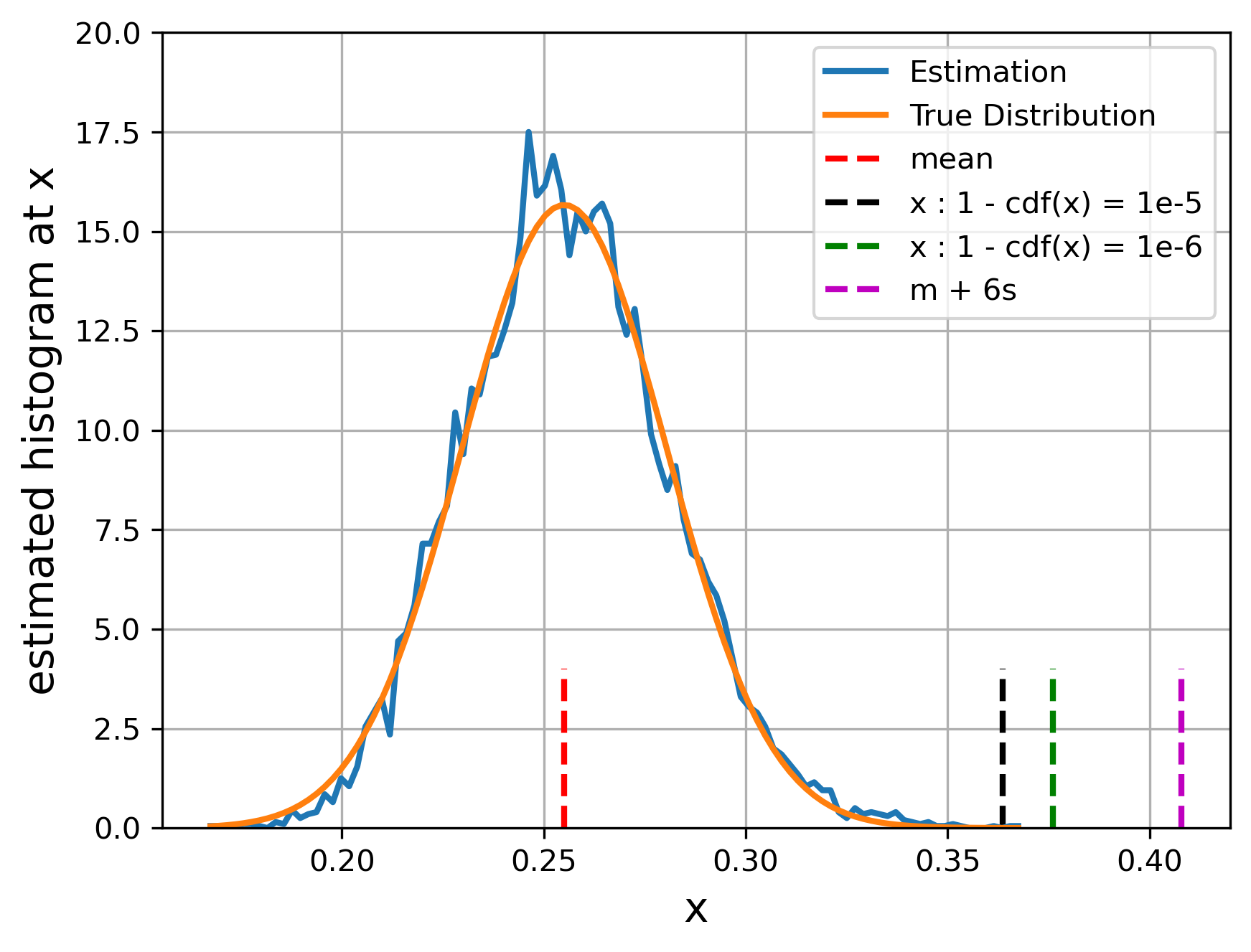
Figure 1: Estimated density probability of $\sum_{i}^{k}Y_{i}$ and the Normal distribution of same mean and standard deviation. Here, we have $k=200$ and $d=784$ which corresponds to the dimensionality of MNIST digits and the number of random projections we use in the experiments. We illustrate also some bounds (on the squared sensitivity) that can be derived from this Normal distribution as well as our CLT bound. Note that the Bernstein bound is above 1 and in this example, that the CLT bound, which is numerically equal to the inverse CDF of the Normal distribution at desired $\delta$.

Proposition 2.

Let $\alpha>1$ and $\delta\in[0,1/2]$, given a random direction projection matrix $\mathbf{U}\in\mathbb{R}^{d\times k}$, then the Gaussian mechanism $\mathcal{M}(\mathbf{X})=\mathbf{X}\mathbf{U}+\mathbf{V}$, where $\mathbf{V}$ is a Gaussian matrix in $\mathbb{R}^{n\times k}$ with entries drawn from $\mathcal{N}(0,\sigma^{2})$ is $(\frac{\alpha{w(k,\delta/2)}}{2\sigma^{2}}+\frac{log(2/\delta)}{\alpha-1},\delta)$-DP.

Proof.

The claim derives immediately by the relation between RDP and DP and by Lemma 2 with $\frac{\delta}{2}$. ∎

The above DP guarantees apply to the full dataset. Hence, when learning through mini-batches, we benefit from the so-called privacy amplification by the “subsampling” principle, which ensures that a differentially private mechanism run on a random subsample of a population leads to higher privacy guarantees than when run on the full population [4]. On the contrary, gradient clipping/sanitization acts individually one each gradient and thus do not fully benefit from the subsampling amplification, as its DP property may still depend on the batch size [9].

This Gaussian mechanism on the random direction projections $\mathcal{M}(\mathbf{X})$ can be related to the definition of the empirical SWD as each $\mathbf{x}_{i}^{\top}\mathbf{u}_{j}$ corresponds to one entry of $\mathbf{X}\mathbf{U}$. Hence, by adding a Gaussian noise to each projection, we naturally derive our empirical DP Sliced Wasserstein distance, which inherits the differential property of $\mathcal{M}(\mathbf{X})$, owing to the post-processing proposition [12].

3.2 Metric Properties of DP-SWD

We have analyzed the sensitivity of the random direction projection central to SWD and we have proposed a Gaussian mechanism to obtain a differentially private SWD (DP-SWD) which steps are depicted in Algorithm 1. In our use-cases, DP-SWD is used in a context of learning to match two distributions (one of them requiring to be privately protected). Hence, the utility guarantees of our DP-SWD is more related to the ability of the mechanism to distinguish two different distributions rather than on the equivalence between SWD and DP-SWD. Our goal in this section is to investigate the impact of adding Gaussian noise to the source $\mu$ and target $\nu$ distributions in terms of distance property in the population case.

Since $\mathcal{R}_{\mathbf{u}}$, as defined in Equation (3), is a push-forward operator of probability distributions, the Gaussian mechanism process implies that the Wasserstein distance involved in SWD compares two 1D probability distributions which are respectively the convolution of a Gaussian distribution and $\mathcal{R}_{\mathbf{u}}\mu$ and $\mathcal{R}_{\mathbf{u}}\nu$. Hence, we can consider DP-SWD uses as a building block the 1D smoothed Wasserstein distance between $\mathcal{R}_{\mathbf{u}}\mu$ and $\mathcal{R}_{\mathbf{u}}\nu$ with the smoothing being ensured by $\mathcal{N}_{\sigma}$ and its formal definition being, for $q\geq 1$,

$$\text{DP}_{\sigma}\text{SWD}_{q}^{q}(\mu,\nu)\doteq\int_{\mathbb{S}^{d-1}}W_{q}^{q}(\mathcal{R}_{\mathbf{u}}\mu*\mathcal{N}_{\sigma},\mathcal{R}_{\mathbf{u}}\nu*\mathcal{N}_{\sigma})u_{d}(\mathbf{u})d\mathbf{u}$$

While some works have analyzed the theoretical properties of the Smoothed Wasserstein distance [15, 14], as far as we know, no theoretical result is available for the smoothed Sliced Wasserstein distance, and we provide in the sequel some insights that help its understanding. The following property shows that DP-SWD preserves the identity of indiscernibles.

Property 1.

For continuous probability distributions $\mu$ and $\nu$, we have, for $q\geq 1$, $\text{DP}_{\sigma}\text{SWD}_{q}^{q}(\mu,\nu)=0\Leftrightarrow\mu=\nu$ $\forall\sigma>0$.

Proof.

Showing that $\mu=\nu\implies\text{DP}_{\sigma}\text{SWD}_{q}^{q}(\mu,\nu)=0$ is trivial as the Radon transform and the convolution are two well-defined maps. We essentially would like to show that $\text{DP}_{\sigma}\text{SWD}_{q}^{q}(\mu,\nu)=0$ implies $\mu=\nu$. If $\text{DP}_{\sigma}\text{SWD}_{q}^{q}(\mu,\nu)=0$ then $\mathcal{R}_{\mathbf{u}}\mu*\mathcal{N}_{\sigma}=\mathcal{R}_{\mathbf{u}}\nu*\mathcal{N}_{\sigma}$ for almost every $\mathbf{u}\in{\mathbb{S}^{d-1}}$. As convolution yields to multiplication in the Fourier domain and because, the Fourier transform of a Gaussian is also a Gaussian and thus is always positive, one can show that we have for all $\mathbf{u}$ equality of the Fourier transforms of $\mathcal{R}_{\mathbf{u}}\mu$ and $\mathcal{R}_{\mathbf{u}}\nu$. Then, owing to the continuity of $\mu$ and $\nu$ and by the Fourier inversion theorem, we have $\mathcal{R}_{\mathbf{u}}\mu=\mathcal{R}_{\mathbf{u}}\nu$. Finally, as for the SWD proof [6, Prop 5.1.2], this implies that $\mu=\nu$, owing to the projection nature of the Radon Transform and because the Fourier transform is injective. ∎

Property 2.

For $q\geq 1$, $\text{DP}_{\sigma}\text{SWD}_{q}^{q}(\mu,\nu)$ is symmetric and satisfies the triangle inequality.

Proof.

The proof easily derives from the metric properties of Smoothed Wasserstein distance [14] and details are in the appendix. ∎

These properties are strongly relevant in the context of our machine learning applications. Indeed, while they do not tell us how the value of DP-SWD compares with SWD, at fixed $\sigma>0$ or when $\sigma\rightarrow 0$, they show that they can properly act as (for any $\sigma>0$) loss functions to minimize if we aim to match distributions (at least in the population case). Naturally, there are still several theoretical properties of $\text{DP}_{\sigma}\text{SWD}_{q}^{q}$ that are worth investigating but that are beyond the scope of this work.

4 DP-Distribution Matching Problems

Algorithm 2 Differentially private DANN with DP-SWD

0:   $\{\mathbf{X}_{s},\mathbf{y}_{s}\},\{\mathbf{X}_{t}\}$, respectively the public and private domain, $\sigma$ standard deviation of the Gaussian mechanism

1:  Initialize representation mapping $g$, the classifier $h$ with parameters $\theta_{g}$, $\theta_{h}$

2:  repeat

3:     sample minibatches $\{x_{B}^{s},y_{B}^{s}\}$ from $\{x_{i}^{s},y_{i}^{s}\}$

4:     compute $g(x_{B}^{s})$

5:     compute the classification loss ${L}_{c}=\sum_{i\in B}L(y_{i}^{s},h(g(x_{i}^{s})))$

6:     $\theta_{h}\leftarrow\theta_{h}-\alpha_{h}\nabla_{\theta_{h}}{L}_{c}$

7:     // Private steps : $g(x_{B}^{t})$ is computed in a private way. $g(\cdot)$ is either transferred or has shared weights between public and private clients.

8:     sample minibatches $\{x_{B}^{t}\}$ from $\{x_{B}^{t}\}$

9:     compute $g(x_{B}^{t})$

10:     normalize each sample $g(x_{B}^{s})$ wrt $2\max_{j}{\|g(x_{B,j}^{s})\|_{2}}$

11:     normalize each sample $g(x_{B}^{t})$ wrt $2\max_{j}{\|g(x_{B,j}^{t})\|_{2}}$

12:     compute $\text{DP}_{\sigma}\text{SWD}(g(x_{B}^{s}),g(x_{B}^{t}))$

13:     publish $\nabla_{\theta_{g}}\text{DP}_{\sigma}\text{SWD}$

14:     // public step

15:     $\theta_{g}\leftarrow\theta_{g}-\alpha_{g}\nabla_{\theta_{g}}L_{c}-\alpha_{g}\nabla_{\theta_{g}}\text{DP}_{\sigma}\text{SWD}$

16:  until a convergence condition is met

There exists several machine learning problems where distance between distributions is the key part of the loss function to optimize. In domain adaptation, one learns a classifier from public source dataset but looks to adapt it to private target dataset (target domain examples are available only through a privacy-preserving mechanism). In generative modelling, the goal is to generate samples similar to true data which are accessible only through a privacy-preserving mechanism. In the sequel, we describe how our $\text{DP}_{\sigma}\text{SWD}_{q}^{q}$ distance can be instantiated into these two learning paradigms for measuring adaptation or for measuring similarity between generated an true samples.

For unsupervised domain adaptation, given source examples $\mathbf{X}_{s}$ and their label $\mathbf{y}_{s}$ and unlabeled private target examples $\mathbf{X}_{t}$, the goal is to learn a classifier $h(\cdot)$ trained on the source examples that generalizes well on the target ones. One usual technique is to learn a representation mapping $g(\cdot)$ that leads to invariant latent representations, invariance being measured as some distance between empirical distributions of mapped source and target samples. Formally, this leads to the following learning problem

$$\min_{g,h}L_{c}(h(g(\mathbf{X}_{s})),\mathbf{y}_{s})+\text{DP}_{\sigma}\text{SWD}(g(\mathbf{X}_{s}),g(\mathbf{X}_{t}))$$ (7)

where $L_{c}$ can be any loss function of interest and $\text{DP}_{\sigma}\text{SWD}=\text{DP}_{\sigma}\text{SWD}_{q}$. We solve this problem through stochastic gradient descent, similarly to many approaches that use Sliced Wasserstein Distance as a distribution distance [20], except that in our case, the gradient of $\text{DP}_{\sigma}\text{SWD}$ involving the target dataset is $(\varepsilon,\delta)$-DP. Note that in order to compute the $\text{DP}_{\sigma}\text{SWD}$, one needs the public dataset $\mathbf{X}_{s}$ and the public generator. In practice, this generator can either be transferred, after each update, from the private client curating $\mathbf{X}_{t}$ or can be duplicated on that client. The resulting algorithm is presented in Algorithm 2.

In the context of generative modeling, we follow the same steps as Deshpande et al. [10] but use our $\text{DP}_{\sigma}\text{SWD}$ instead of SWD. Assuming that we have some examples of data $\mathbf{X}_{t}$ sampled from a given distribution, the goal of the learning problem is to learn a generator $g(\cdot)$ to output samples similar to those of the target distribution, with at its input a given noise vector. This is usually achieved by solving

$$\min_{g}\text{DP}_{\sigma}\text{SWD}(\mathbf{X}_{t},g(z))$$ (8)

where $z$ is for instance a Gaussian vector. In practice, we solve this problem using a mini-batching stochastic gradient descent strategy, following a similar algorithm than the one for domain adaptation. The main difference is that the private target dataset does not pass through the generator.

Tracking the privacy loss

Given that we consider the privacy mechanism within a stochastic gradient descent framework, we keep track of the privacy loss through the RDP accountant proposed by Wang et al. [32] for composing subsampled private mechanisms. Hence, we used the PyTorch package [33] that they made available for estimating the noise standard deviation $\sigma$ given the $(\varepsilon,\delta)$ budget, a number of epoch, a fixed batch size, the number of private samples, the dimension $d$ of the distributions to be compared and the number $k$ of projections used for $\text{DP}_{\sigma}\text{SWD}$. Some examples of Gaussian noise standard deviation are reported in Table 4 in the appendix.

5 Related Works

5.1 DP Generative Models

Most recent approaches [13] that proposed DP generative models considered it from a GAN perspective and applied DP-SGD [1] for training the model. The main idea for introducing privacy is to appropriately clip the gradient and to add calibrated noise into the model’s parameter gradient during training [29, 9, 34]. This added noise make those models even harder to train. Furthermore, since the DP mechanism applies to each single gradient, those approaches do not fully benefit from the amplification induced by subsampling (mini-batching) mechanism [4]. The work of Chen et al. [9] uses gradient sanitization and achieves privacy amplification by training multiple discriminators, as in [18], and sampling on them for adversarial training. While their approach is competitive in term of quality of generated data, it is hardly tractable for large scale dataset, due to the multiple (up to 1000 in their experiments) discriminator trainings.

Instead of considering adversarial training, some DP generative model works have investigated the use of distance on distributions. Harder et al. [17] proposed random feature based maximum-mean embedding distance for computing distance between empirical distributions. Cao et al. [7] considered the Sinkhorn divergence for computing distance between true and generated data and used gradient clipping and noise addition for privacy preservation. Their approach is then very similar to DP-SGD in the privacy mechanism. Instead, we perturb the Sliced Wasserstein distance by smoothing the distributions to compare. This yields a privacy mechanism that benefits subsampling amplification, as its sensitivity does not depend on the number of samples, and that preserves its utility as the smoothed Sliced Wasserstein distance is still a distance.

5.2 Differential Privacy with Random Projections

Sliced Wasserstein Distance leverages on Radon transform for mapping high-dimensional distributions into 1D distributions. This is related to projection on random directions and the sensitivity analysis of those projections on unit-norm random vector is key. The first use of random projection for differential privacy has been introduced by Kenthapadi et al. [19]. Their approach was linked to the distance preserving property of random projections induced by the Johnson-Lindenstrauss Lemma. As a natural extension, LeTien et al. [21] and Gondara & Wang [16] have applied this idea in the context of optimal transport and classification. The fact that we project on unit-norm random vector, instead of any random vector as in Kenthapadi et al. [19], requires a novel sensitivity analysis and we show that this sensitivity scales gracefully with ratio of the number of projections and dimension of the distributions.

6 Numerical Experiments

In this section, we provide some numerical results showing how our differentially private Sliced Wasserstein Distance works in practice. The code for reproducing some of the results is available in https://github.com/arakotom/dp_swd.

6.1 Toy Experiment

The goal of this experiment is to illustrate the behaviour of the DP-SWD compared with the SWD in controlled situations. We consider the source and target distributions as isotropic Normal distributions of unit variance with added privacy-inducing Gaussian noise of different variances. Both distributions are Gaussian of dimension $5$ and the means of the source and target are respectively $\mathbf{m}_{\mu}=0$ and $\mathbf{m}_{\nu}=c1$ with $c\in[0,1]$. Figure 2 presents the evolution of the distances averaged over $5$ random draws of the Gaussian and noise. When source and target distributions are different, this experiment shows that DP-SWD follows the same increasing trend as SWD. This suggests that the order relation between distributions as evaluated using SWD is preserved by DP-SWD, and that the distance DP-SWD is minimized when $\mu=\nu$, which are important features when using DP-SWD as a loss.

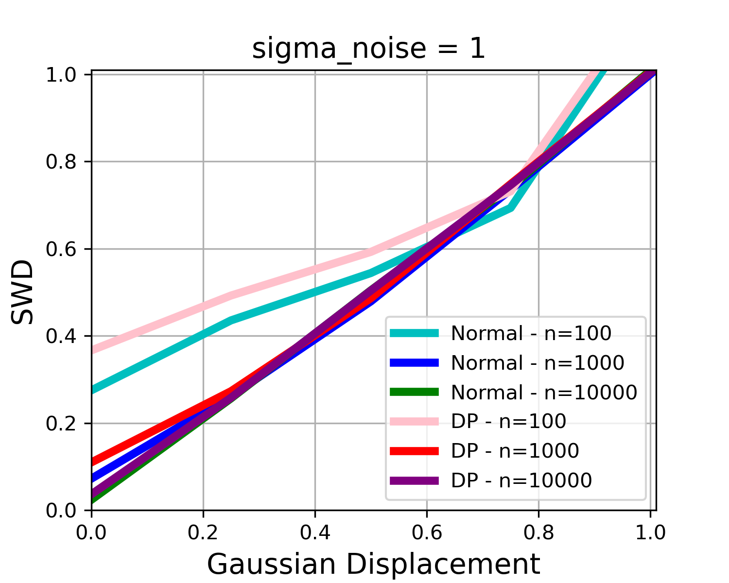
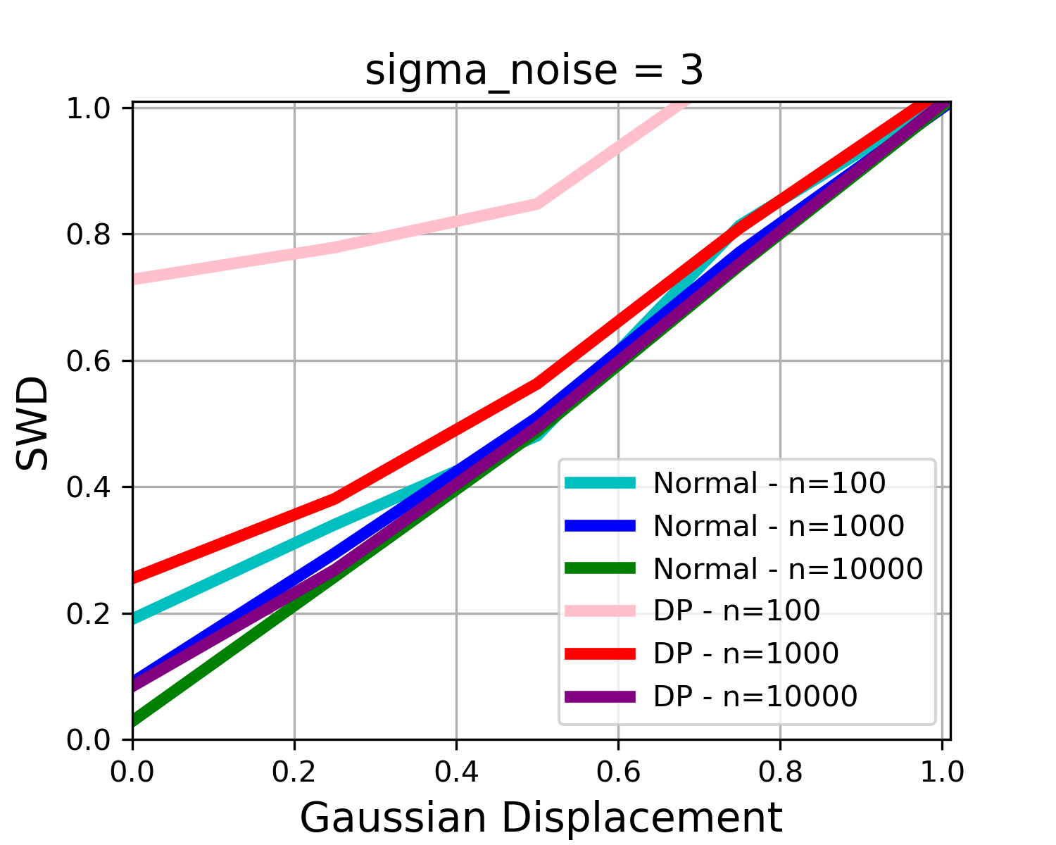
Figure 2: Comparing SWD and DP-SWD by measuring the distance between two normal distributions (averaged over $5$ draws of all samples). The comparison holds when the distance between the means of the Gaussians increases linearly, for different noise amplitudes of the Gaussian mechanism and different number of samples. (left) $\sigma=1$. (right) $\sigma=3$.

6.2 Domain Adaptation

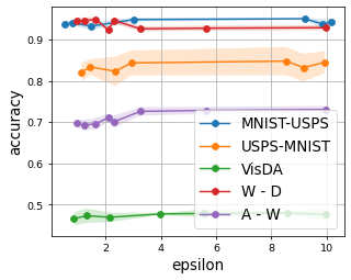
Figure 3: Evolution of the target domain accuracy in UDA with respect to the $\varepsilon$ parameter for fixed value of $\delta$, for $3$ different datasets. Sensitivity of DP-SWD has been computed using the Bernstein bound.

We conduct experiments for evaluating our DP-SWD distance in the context of classical unsupervised domain adaptation (UDA) problems such as handwritten digit recognitions (MNIST/USPS), synthetic to real object data (VisDA 2017) and Office 31 datasets. Our goal is to analyze how DP-SWD performs compared with its public counterpart SWD [20], with one DP deep domain adaptation algorithm DP-DANN that is based on gradient clipping [31] and with the classical non-private DANN algorithm. Note that we need not compare with [21] as their algorithm does not learn representation and does not handle large-scale problems, as the OT transport matrix coupling need be computed on the full dataset. For all methods and for each dataset, we used the same neural network architecture for representation mapping and for classification. Approaches differ only on how distance between distributions have been computed. Details of problem configurations as well as model architecture and training procedure can be found in the appendix. Sensitivity has been computed using the Bernstein bound of Lemma 2.

Table 1 presents the accuracy on the target domain for all methods averaged over $10$ iterations. We remark that our private model outperforms the DP-DANN approach on all problems except on two difficult ones. Interestingly, our method does not incur a loss of performance despite the private mechanism. This finding is confirmed in Figure 3 where we plot the performance of the model with respect to the noise level $\sigma$ (and thus the privacy parameter $\varepsilon$). Our model is able to keep accuracy almost constant for $\varepsilon\in[3,10]$.

Table 1: Table of accuracy on the private target domain for different domain adaptation problems M-U, U-M refers to MNIST-USPS and USPS-MNIST the first listed data being the source domain. (D,W,A) refers to domains in the Office31 dataset. For all the problems, $\varepsilon=10$ and $\delta$ depends on the number of examples in target domain. $\delta$ has been respectively set to $10^{-3}$,$10^{-5}$,$10^{-6}$ for Office31, MNIST-USPS and VisDA.

	Methods
Data	DANN	SWD	DP-DANN	DP-SWD
M-U	93.9 $\pm$ 0	95.5 $\pm$ 1	87.1 $\pm$ 2	94.0$\pm$ 0
U-M	86.2 $\pm$ 2	84.8$\pm$2	73.5 $\pm$ 2	83.4$\pm$ 2
VisDA	57.4 $\pm$ 1	53.8$\pm$1	49.0 $\pm$ 1	47.0$\pm$ 1
D - W	90.9$\pm$ 1	90.7$\pm$ 1	88.0$\pm$ 1	90.9$\pm$ 1
D - A	58.6$\pm$ 1	59.4$\pm$ 1	56.5$\pm$ 1	55.2$\pm$ 2
A - W	70.4$\pm$ 3	74.5$\pm$ 1	68.7$\pm$ 1	72.6$\pm$ 1
A - D	78.6$\pm$ 2	78.5$\pm$ 1	73.7$\pm$ 1	79.8$\pm$ 1
W - A	54.7$\pm$ 3	59.1$\pm$ 0	56.0$\pm$ 1	59.0$\pm$ 1
W - D	91.1$\pm$ 0	95.7$\pm$ 1	63.4$\pm$ 3	92.6$\pm$ 1

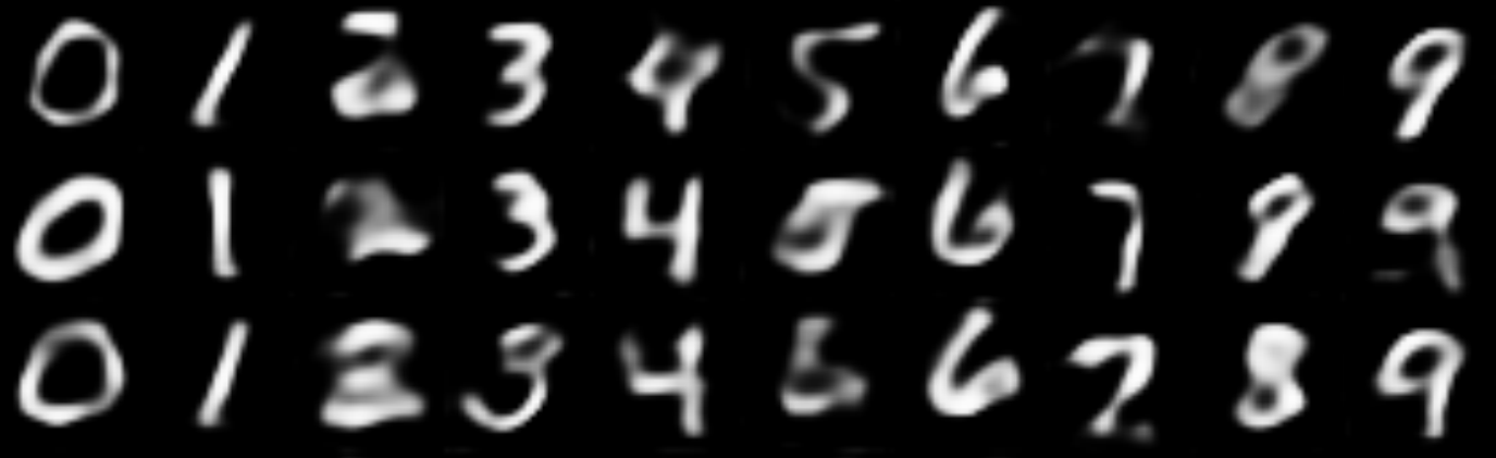
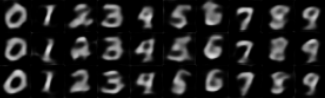
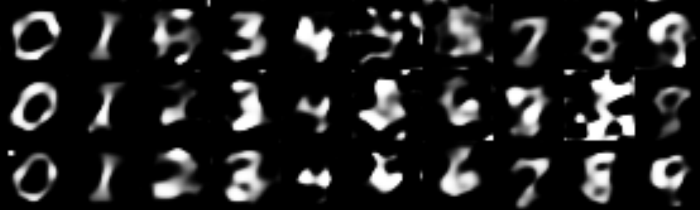
Figure 4: Examples of generate MNIST samples from (top) non-private SWD (middle) DP-SWD-b (bottom) MERF.

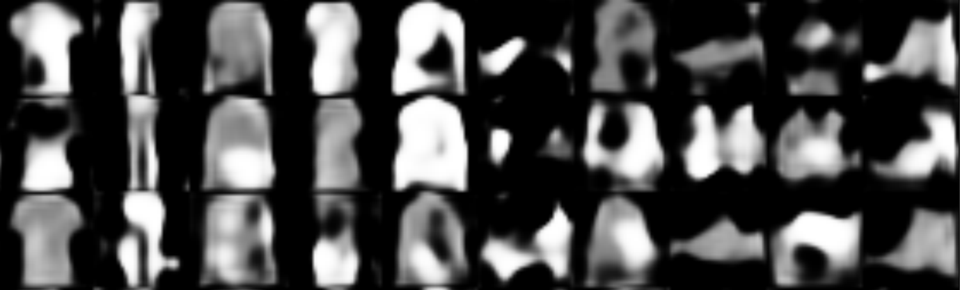
Figure 5: Examples of generate FashionMNIST samples from (top) non-private SWD (middle) DP-SWD-b (bottom) MERF.

6.3 Generative Models

Table 2: Comparison of DP generative models on MNIST and FashionMNIST at privacy level $(\varepsilon,\delta)=(10,10^{-5})$. The downstream task is a $10$-class classification problems using the synthetic generated dataset. We report the accuracy of different classifiers. Results are averaged over $5$ runs of generation. SWD is the non-private version of our generative model.

	MNIST		FashionMNIST
Method	MLP	LogReg	MLP	LogReg
SWD	87	82	77	76
GS-WGAN	79	79	65	68
DP-CGAN	60	60	50	51
DP-MERF	76	75	72	71
DP-SWD-c	77	78	67	66
DP-SWD-b	76	77	67	66

In the context of generative models, our first task is to generate synthetic samples for MNIST and Fashion MNIST dataset that will be afterwards used for learning a classifier. We compare with different gradient-sanitization strategies like DP-CGAN [29], and GS-WGAN [9] and a model MERF [17] that uses MMD as distribution distance. We report results for our DP-SWD using two ways for computing the sensitivity, by using the CLT bound and the Bernstein bound, respectively noted as DP-SWD-c and DP-SWD-b. All models are compared with the same fixed budget of privacy $(\varepsilon,\delta)=(10,10^{-5})$. Our implementation is based on the one of MERF [17], in which we just plugged our DP-SWD loss in place of the MMD loss. The architecture of ours and MERF’s generative model is composed of few layers of convolutional neural networks and upsampling layers with approximately 180K parameters while the one of GS-WGAN is based on a ResNet with about 4M parameters. MERF’s and our models have been trained over $100$ epochs with an Adam optimizer and batch size of $100$. For our DP-SWD we have used $1000$ random projections and the output dimension is the classical $28\times 28=784$.

Table 2 reports some quantitative results on the task. We note that MERF and our DP-SWD perform on par on these problems (with a slight advantage for MERF on FashionMNIST and for DP-SWD on MNIST). Note that our results on MERF are better than those reported in [9]. We also remark that GS-WGAN performs the best at the expense of a model with $20$-fold more parameters and a very expensive training time (few hours just for training the $1000$ discriminators, while our model and MERF’s take less than 10min). Figure 4 and 5 present some examples of generated samples for MNIST and FashionMNIST. We can note that the samples generated by DP-SWD present some diversity and are visually more relevant than those of MERF, although they do not lead to better performance in the classification task. Our samples are a bit blurry compared to the ones generated by the non-private SWD: this is an expected effect of smoothing.

We also evaluate our DP-SWD distance for training generative models on large RGB datasets such as the $64\times 64\times 3$ CelebA dataset. To the best of our knowledge, no DP generative approaches have been experimented on such a dataset. For instance, the GS-WGAN of [9] has been evaluated only on grayscale MNIST-like problems. For training the model, we followed the same approach (architecture and optimizer) as the one described in Nguyen et al. [23]. In that work, in order to reduce the dimension of the problems, distributions are compared in a latent space of dimension $d=8192$. We have used $k=2000$ projections which leads to a ratio $\frac{k}{d}<0.25$. Noise variance $\sigma$ and privacy loss over $100$ iterations have been evaluated using the PyTorch package of [32] and have been calibrated for $\epsilon=10$ and $\delta=10^{-6}$, since the number of training samples is of the order of $170$K. Details are in the appendix. Figure 6 presents some examples of samples generated from our DP-SWD and SWD. We note that in this high-dimensional context, the sensitivity bound plays a key role, as we get a FID score of 97 vs 158 respectively using CLT bound and Bernstein bound, the former being smaller than the latter.

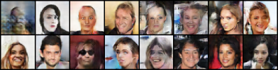
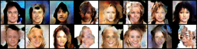
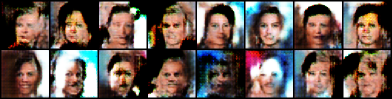
Figure 6: Images generated on CelebA dataset. From top to bottom. Non-private SWD, DP-SWD with noise calibrated according to Gaussian approximation (CLT bound), DP-SWD with noise calibrated according to the Bernstein bound. The FID score computed over $10000$ generated examples of this three models are respectively $58$, $97$ and $149$.

7 Conclusion

This paper presents a differentially private distance on distributions based on the sliced Wasserstein distance. We applied a Gaussian mechanism on the random projection inherent to SWD and analyzed its properties. We proved that a bound (à la Bernstein) on sensitivity of the mechanism as an inverse dependence on the problem dimension and that a Central limit theorem bound, although approximate, gives a tighter bound. One of our key findings is that the privacy-inducing mechanism we proposed turns the SWD into a smoothed sliced Wasserstein distance, which inherits all the properties of a distance. Hence, our privacy-preserving distance can be plugged seamlessly into domain adaptation or generative model algorithms to give effective privacy-preserving learning procedures.

Supplementary material
Differentially Private Sliced Wasserstein Distance

8 Appendix

8.1 Lemma 1 and its proof

Lemma 1.

Assume that $\mathbf{z}\in\mathbb{R}^{d}$ is a unit-norm vector and $\mathbf{u}\in\mathbb{R}^{d}$ a vector where each entry is drawn independently from $\mathcal{N}(0,\sigma_{u}^{2})$. Then

$$Y\doteq\Big{(}\mathbf{z}^{\top}\frac{\mathbf{u}}{\|\mathbf{u}\|_{2}}\Big{)}^{2}\sim B(1/2,(d-1)/2)$$

where $B(\alpha,\beta)$ is the beta distribution of parameters $\alpha,\beta$.

Proof.

At first, consider a vector of unit-length in $\mathbb{R}^{d}$, say $\mathbf{e}_{1}$, that can be completed to an orthogonal basis. A change of basis from the canonical one does not change the length of a vector as the transformation is orthogonal. Thus the distribution of

$$\frac{(\mathbf{e}_{1}^{\top}\mathbf{u})^{2}}{\|\mathbf{u}\|_{2}^{2}}=\frac{(\mathbf{e}_{1}^{\top}\mathbf{u})^{2}}{\sum_{i}^{d}u_{i}^{2}}$$

does not depend on $\mathbf{e}_{1}$. $\mathbf{e}_{1}$ can be either the vector $(1,0,\cdots,0)$ in $\mathbb{R}^{d}$ or $\mathbf{z}$ (as $\mathbf{z}$ is an unit-norm vector). However, for simplicity, let us consider $\mathbf{e}_{1}$ as $(1,0,\cdots,0)$, we thus have

$$\frac{(\mathbf{e}_{1}^{\top}\mathbf{u})^{2}}{\|\mathbf{u}\|_{2}^{2}}=\frac{u_{1}^{2}}{\sum_{i}^{d}u_{i}^{2}}$$

where the $u_{i}$ are iid from a normal distribution of standard deviation $\sigma_{u}$. Hence, because $u_{1}$ and the $\{u_{i}\}_{i=2}^{d}$ are independent, the above distribution is equal to the one of

$$\frac{\sigma_{u}^{2}V}{\sigma_{u}^{2}V+\sigma_{u}^{2}Z}$$

where $V=u_{1}^{2}/\sigma_{u}^{2}\sim\Gamma(1/2)$ (and is a chi-square distribution) ) and $Z=(\sum_{i=2}^{d}u_{i}^{2})/\sigma_{u}^{2}\sim\Gamma((d-1)/2)$ and thus $V/(V+Z)$ follows a beta distribution $B(1/2,(d-1)/2)$. And the fact that $\mathbf{z}$ is also a unit-norm vector concludes the proof.

∎

A simulation of the random $Y$ and resulting histogram is depicted in Figure 7.

Remark 3.

From the properties of the beta distribution, expectation and variances are given by

$$\operatorname{\mathbb{E}}Y=\frac{1}{d}\quad\text{and}\quad\operatorname{\mathbb{V}}Y=\frac{2(d-1)}{d^{2}(d+2)}$$

Remark 4.

Note that if $\mathbf{z}$ is not of unit-length then $Y$ follows $\|\mathbf{z}\|B(1/2,(d-1)/2)$

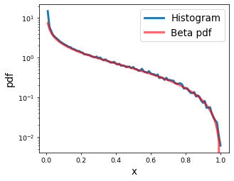
Figure 7: Estimation of the pdf of $Y$ in Lemma 1, for a fixed $\mathbf{z}$, based on a histogram over $100000$ samples of $\mathbf{u}$. Here, we have $d=5$.

8.2 Lemma 2 and its proof

Lemma 2.

Suppose again that $\mathbf{z}$ is unit norm. With probability at least $1-\delta$, we have

$$\left\|\mathbf{X}\mathbf{U}-\mathbf{X}^{\prime}\mathbf{U}\right\|_{F}^{2}\leq w(k,\delta),$$ (9)

with

$$w(k,\delta)\doteq\frac{k}{d}+\frac{2}{3}\ln\frac{1}{\delta}+\frac{2}{d}\sqrt{k\frac{d-1}{d+2}\ln\frac{1}{\delta}}$$ (10)

Proof.

First observe that:

$$H \doteq\left\|\mathbf{X}\mathbf{U}-\mathbf{X}^{\prime}\mathbf{U}\right\|_{F}^{2}=\left\|(\mathbf{X}-\mathbf{X}^{\prime})\mathbf{U}\right\|_{F}^{2}$$

$$=\left\|\mathbf{z}^{\top}\mathbf{U}\right\|_{2}^{2}=\sum_{j=1}^{k}\left(\mathbf{z}^{\top}\frac{\mathbf{u}_{j}}{\|\mathbf{u}_{j}\|}\right)^{2}$$

$$=\sum_{j=1}^{k}Y_{j},\text{ where }Y_{j}\doteq\left(\mathbf{z}^{\top}\frac{\mathbf{u}_{j}}{\|\mathbf{u}_{j}\|}\right)^{2}.$$

Therefore, $H$ is the sum of $k$ iid $B(1/2,(d-1)/2)$-distributed random variables.

It is thus possible to use any inequality bounding $H$ from its mean to state a highly probable interval for $H$. We here use inequality, that is tighter than Hoeffding inequality, whenever some knowledge is provided on the variance of the random variables considered. Recall that it states that if $Y_{1},\ldots,Y_{k}$ and zero-mean independent RV with such that $|Y_{i}|\leq M$ a.s:

$$\mathbf{P}\left(\sum_{j=1}^{k}Y_{j}\geq t\right)\leq\exp\left(-\frac{t^{2}}{2\sum_{j=1}^{k}\mathbf{E}Y_{j}^{2}+\frac{2}{3}Mt}\right)$$

For $H$, we have

$$\mathbf{E}H=\sum_{j=1}^{k}\mathbf{E}\left(\mathbf{z}^{\top}\frac{\mathbf{u}_{j}}{\|\mathbf{u}_{j}\|}\right)^{2}=\sum_{j=1}^{k}\frac{1}{d}=\frac{k}{d}$$

and Bernstein’s inequality gives

$$\mathbf{P}\left(H\geq\frac{k}{d}+t\right)\leq\exp\left(-\frac{t^{2}}{2kv_{d}+\frac{2}{3}t}\right),$$

where

$$v_{d}=\frac{2(d-1)}{d^{2}(d+2)}$$

is the variance of each $(\mathbf{z}^{\top}\mathbf{u}_{j}/\|\mathbf{u}_{j}\|)^{2}$ beta distributed variable. Making the right hand side be equal to $\delta$, solving the second-order equation for $t$ give that, with probability at least $1-\delta$

$$H\leq\frac{k}{d}+\frac{2}{3}\ln\frac{1}{\delta}+\sqrt{2kv_{d}\ln\frac{1}{\delta}}$$

The proof follows directly from Lemma 1 and the fact ∎

From the above lemma, we have a probabilistic bound on the sensitivity of the random direction projection and SWD . The lower this bound is the better it is, as less noise needed for achieving a certain $(\varepsilon,\delta)$-DP. Interestingly, the first and last terms in this bound have an inverse dependency on the dimension. Hence, if the dimension of space in which the DP-SWD has to be chosen, for instance, when considering latent representation, a practical compromise has to be performed between a smaller bound and a better estimation. Also remark that if $k<d$, the bound is mostly dominated by the term $\log(1/\delta)$. Compared to other random-projection bounds [30] which have a linear dependency in $k$. For our bound, dimension also help in mitigating this dependency.

8.3 Proof of the Central Limit Theorem based bound

Proof.

Proof with the Central Limit Theorem According to the Central Limit Theorem — whenever $k>30$ is the accepted rule of thumb — we may consider that

$$\frac{H}{k}\sim{\cal N}\left(\frac{1}{d},\frac{v_{d}}{k}\right)$$

i.e.

$$\left(\frac{H}{k}-\frac{1}{d}\right)\sqrt{\frac{k}{v_{d}}}\sim{\cal N}(0,1)$$

and thus

$$\mathbf{P}\left(\left(\frac{H}{k}-\frac{1}{d}\right)\sqrt{\frac{k}{v_{d}}}\geq t\right)\leq 1-\Phi(t)$$

Setting $1-\Phi(t)=\delta$ gives $t=\Phi^{-1}(1-\delta)\doteq z_{1-\delta}$, and thus with probability at least $1-\delta$

$$H \leq\frac{k}{d}+z_{1-\delta}\sqrt{k{v_{d}}}$$

$$=\frac{k}{d}+\frac{z_{1-\delta}}{d}\sqrt{\frac{2k(d-1)}{d+2}}$$

∎

8.4 Proof of Property 2.

Property 2.

$\text{DP}_{\sigma}\text{SWD}_{q}^{q}(\mu,\nu)$ is symmetric and satisfies the triangle inequality for $q=1$.

Proof.

The symmetry trivially comes from the definition of $\text{DP}_{\sigma}\text{SWD}_{q}^{q}(\mu,\nu)$ that is

$$\text{DP}_{\sigma}\text{SWD}_{q}^{q}(\mu,\nu)=\mathbf{E}_{\mathbf{u}\sim\mathbb{S}^{d-1}}W_{q}^{q}(\mathcal{R}_{\mathbf{u}}\mu*\mathcal{N}_{\sigma},\mathcal{R}_{\mathbf{u}}\nu*\mathcal{N}_{\sigma})$$

and the fact the Wasserstein distance is itself symmetric.

Regarding the triangle inequality for $q\geq 1$, our result is based on a very recent result showing that the smoothed Wasserstein for $q\geq 1$ is also a metric [25] (Our proof is indeed valid for $q\geq 1$, as this recent result generalizes the one of [14] ). Hence, we have

$$\text{DP}_{\sigma}\text{SWD}_{q}(\mu,\nu) =\Big{[}\mathbf{E}_{\mathbf{u}\sim\mathbb{S}^{d-1}}W_{q}^{q}(\mathcal{R}_{\mathbf{u}}\mu*\mathcal{N}_{\sigma},\mathcal{R}_{\mathbf{u}}\nu*\mathcal{N}_{\sigma})\Big{]}^{1/q}$$

$$\leq\Big{[}\mathbf{E}_{\mathbf{u}\sim\mathbb{S}^{d-1}}\big{(}W_{q}(\mathcal{R}_{\mathbf{u}}\mu*\mathcal{N}_{\sigma},\mathcal{R}_{\mathbf{u}}\xi*\mathcal{N}_{\sigma})$$

$$+W_{q}(\mathcal{R}_{\mathbf{u}}\xi*\mathcal{N}_{\sigma},\mathcal{R}_{\mathbf{u}}\nu*\mathcal{N}_{\sigma})\big{)}^{q}\Big{]}^{1/q}$$

$$\leq\Big{[}\mathbf{E}_{\mathbf{u}\sim\mathbb{S}^{d-1}}W_{q}^{q}(\mathcal{R}_{\mathbf{u}}\mu*\mathcal{N}_{\sigma},\mathcal{R}_{\mathbf{u}}\xi*\mathcal{N}_{\sigma})\Big{]}^{1/q}$$

$$+\Big{[}\mathbf{E}_{\mathbf{u}\sim\mathbb{S}^{d-1}}W_{q}^{q}(\mathcal{R}_{\mathbf{u}}\xi*\mathcal{N}_{\sigma},\mathcal{R}_{\mathbf{u}}\nu*\mathcal{N}_{\sigma})\Big{]}^{1/q}$$

$$\leq\text{DP}_{\sigma}\text{SWD}_{q}(\mu,\xi)+\text{DP}_{\sigma}\text{SWD}_{q}(\xi,\nu)\hfill~{}$$

where the first inequality comes from the fact that the smoothed Wassertein distance $W_{q}(\mu*\mathcal{N}_{\sigma},\nu*\mathcal{N}_{\sigma})$ is a metric and satisfies the triangle inequality and the second one follows from the application of the Minkowski inequality.

∎

8.5 Experimental set-up

8.5.1 Dataset details

We have considered $3$ families of domain adaptation problems based on Digits, VisDA, Office-31. For all these datasets, we have considered the natural train/test number of examples.

For the digits problem, we have used the MNIST and the USPS datasets. For MNIST-USPS and USPS-MNIST, we have respectively used 60000-7438, 7438-10000 samples. The VisDA 2017 problem is a $12$-class classification problem with source and target domains being simulated and real images. The Office-31 is an object categorization problem involving $31$ classes with a total of 4652 samples. There exists $3$ domains in the problem based on the source of the images : Amazon (A), DSLR (D) and WebCam (W). We have considered all possible pairwise source-target domains.

For the VisDA and Office datasets, we have considered Imagenet pre-trained ResNet-50 features and our feature extractor (which is a fully-connected feedforword networks) aims at adapting those features. We have used pre-trained features freely available at https://github.com/jindongwang/transferlearning/blob/master/data/dataset.md.

8.5.2 Architecture details for domain adaptations

Digits

For the MNIST-USPS problem, the architecture of our feature extractor is composed of the two CNN layers with 32 and 20 filters of size $5\times 5$. The feature extractor uses a ReLU activation function a max pooling at the first layer and a sigmoid activation function at the second one. For the classification head, we have used a 2-layer fully connected networks as a classifier with $100$ and $10$ units.

VisDA

For the VisDA dataset, we have considered pre-trained 2048 features obtained from a ResNet-50 followed by $2$ fully connected networks with $100$ units and ReLU activations. The latent space is thus of dimension $100$. Discriminators and classifiers are also a $2$ layer fully connected networks with $100$ and respectively 1 and “number of class” units.

Office 31

For the Office dataset, we have considered pre-trained 2048 features obtained from a ResNet-50 followed by two fully connected networks with output of $100$ and $50$ units and ReLU activations. The latent space is thus of dimension $50$. Discriminators and classifiers are also a $2$ layer fully connected networks with $50$ and respectively 1 and “number of class” units.

For Digits, VisDA and Office 31 problems, all models have been trained using Adam with learning rate validated on the non-private model.

8.5.3 Architecture details for generative modelling.

For the MNIST, FashionMNIST generative modelling problems, we have used the implementation of MERF available at https://github.com/frhrdr/dp-merf and plugged in our $\text{DP}_{\sigma}\text{SWD}$ distance. The generator architecture we used is the same as theirs and detailed in Table 3. The optimizer is an Adam optimizer with the default $0.0001$ learning rate. The code dimension is $10$ and is concatenated with the one-hot encoding of the $10$ class label, leading to an overall input distribution of $20$.

For the CelebA generative modelling, we used the implementation of Nguyen et al. [24] available at https://github.com/VinAIResearch/DSW. The generator mixes transpose convolution and batch normalization as described in Table 5. The optimizer is an Adam optimizer with a learning rate of $0.0005$. Again, we have just plugged in our $\text{DP}_{\sigma}\text{SWD}$ distance.

Table 3: Description of the generator for the MNIST and FashionMNIST dataset.  

Module	Parameters
FC	20 - 200
BatchNorm	$\epsilon=10^{-5}$, momentum=0.1
FC	200 - 784
BatchNorm	$\epsilon=10^{-5}$, momentum=0.1
Reshape	28 x 28
upsampling	factor = 2
Convolution	5 x 5 + ReLU
Upsampling	factor = 2
Convolution	5 x 5 + Sigmoid

Table 4: Model hyperparameters and privacy for achieving a $\varepsilon-\delta$ privacy with $\varepsilon=10$ and $\delta$ depending on the size of the private dataset. The four first lines refers to the domain adaptation problems and the data to protect is the private one. The last two rows refer to the generative modelling problems. The noise $\sigma$ has been obtained using the RDP based moment accountant of Xiang [33].

data	$\delta$	$d$	$k$	N	#epoch	batch size	$\sigma$
U-M	$10^{-5}$	784	200	10000	100	128	4.74
M-U	$10^{-5}$	784	200	7438	100	128	5.34
VisDA	$10^{-5}$	100	1000	55387	50	128	6.40
Office	$10^{-3}$	50	100	497	50	32	8.05
MNIST (b)	$10^{-5}$	784	1000	60000	100	100	2.94
MNIST (c)	$10^{-5}$	784	1000	60000	100	100	0.84
CelebA (b)	$10^{-6}$	8192	2000	162K	100	256	2.392
CelebA (c)	$10^{-6}$	8192	2000	162K	100	256	0.37

Table 5: Description of the generator for the CelebA dataset. The input code is of size $32$ and the output is $64\times 64\times 3$.  

Module	Parameters
Transpose Convolution	32 - 512, kernel = 4x4, stride = 1
BatchNorm	$\epsilon=10^{-5}$, momentum=0.1
ReLU
Transpose Convolution	512 - 256, kernel = 4x4, stride = 1
BatchNorm	$\epsilon=10^{-5}$, momentum=0.1
ReLU
Transpose Convolution	256 - 128, kernel = 4x4, stride = 1
BatchNorm	$\epsilon=10^{-5}$, momentum=0.1
ReLU
Transpose Convolution	128 - 64, kernel = 4x4, stride = 1
BatchNorm	$\epsilon=10^{-5}$, momentum=0.1
ReLU
Transpose Convolution	64 - 3, kernel = 4x4, stride = 1
BatchNorm	$\epsilon=10^{-5}$, momentum=0.1
Tanh

References

- Abadi et al. [2016] Abadi, M., Chu, A., Goodfellow, I., McMahan, H. B., Mironov, I., Talwar, K., and Zhang, L. Deep learning with differential privacy. In Proceedings of the 2016 ACM SIGSAC Conference on Computer and Communications Security, pp. 308–318, 2016.
- Asoodeh et al. [2020] Asoodeh, S., Liao, J., Calmon, F. P., Kosut, O., and Sankar, L. Three variants of differential privacy: Lossless conversion and applications. arXiv preprint arXiv:2008.06529, 2020.
- Balle & Wang [2018] Balle, B. and Wang, Y.-X. Improving the Gaussian mechanism for differential privacy: Analytical calibration and optimal denoising. In Dy, J. and Krause, A. (eds.), Proceedings of the 35th International Conference on Machine Learning, volume 80 of Proceedings of Machine Learning Research, pp. 394–403, Stockholmsmässan, Stockholm Sweden, 10–15 Jul 2018. PMLR. URL http://proceedings.mlr.press/v80/balle18a.html.
- Balle et al. [2018] Balle, B., Barthe, G., and Gaboardi, M. Privacy amplification by subsampling: Tight analyses via couplings and divergences. In Bengio, S., Wallach, H., Larochelle, H., Grauman, K., Cesa-Bianchi, N., and Garnett, R. (eds.), Advances in Neural Information Processing Systems, volume 31, pp. 6277–6287. Curran Associates, Inc., 2018. URL https://proceedings.neurips.cc/paper/2018/file/3b5020bb891119b9f5130f1fea9bd773-Paper.pdf.
- Bonneel et al. [2015] Bonneel, N., Rabin, J., Peyré, G., and Pfister, H. Sliced and radon wasserstein barycenters of measures. Journal of Mathematical Imaging and Vision, 51(1):22–45, 2015.
- Bonnotte [2013] Bonnotte, N. Unidimensional and evolution methods for optimal transportation. PhD thesis, Paris 11, 2013.
- Cao et al. [2021] Cao, T., Bie, A., Kreis, K., and Fidler, S. Differentially private generative models through optimal transport, 2021. URL https://openreview.net/forum?id=zgMPc_48Zb.
- Chaudhuri et al. [2011] Chaudhuri, K., Monteleoni, C., and Sarwate, A. D. Differentially private empirical risk minimization. Journal of Machine Learning Research, 12(3), 2011.
- Chen et al. [2020] Chen, D., Orekondy, T., and Fritz, M. Gs-wgan: A gradient-sanitized approach for learning differentially private generators. In Neural Information Processing Systems (NeurIPS), 2020.
- Deshpande et al. [2018] Deshpande, I., Zhang, Z., and Schwing, A. G. Generative modeling using the sliced wasserstein distance. In Proceedings of the IEEE conference on computer vision and pattern recognition, pp. 3483–3491, 2018.
- Dwork [2008] Dwork, C. Differential privacy: A survey of results. In International conference on theory and applications of models of computation, pp. 1–19. Springer, 2008.
- Dwork et al. [2014] Dwork, C., Roth, A., et al. The algorithmic foundations of differential privacy. Foundations and Trends in Theoretical Computer Science, 9(3-4):211–407, 2014.
- Fan [2020] Fan, L. A survey of differentially private generative adversarial networks. In The AAAI Workshop on Privacy-Preserving Artificial Intelligence, 2020.
- Goldfeld & Greenewald [2020] Goldfeld, Z. and Greenewald, K. Gaussian-smoothed optimal transport: Metric structure and statistical efficiency. In International Conference on Artificial Intelligence and Statistics, pp. 3327–3337. PMLR, 2020.
- Goldfeld et al. [2020] Goldfeld, Z., Greenewald, K., and Kato, K. Asymptotic guarantees for generative modeling based on the smooth wasserstein distance. Advances in Neural Information Processing Systems, 33, 2020.
- Gondara & Wang [2020] Gondara, L. and Wang, K. Differentially private small dataset release using random projections. In Conference on Uncertainty in Artificial Intelligence, pp. 639–648. PMLR, 2020.
- Harder et al. [2020] Harder, F., Adamczewski, K., and Park, M. Differentially private mean embeddings with random features (dp-merf) for simple & practical synthetic data generation. arXiv preprint arXiv:2002.11603, 2020.
- Jordon et al. [2018] Jordon, J., Yoon, J., and Van Der Schaar, M. Pate-gan: Generating synthetic data with differential privacy guarantees. In International Conference on Learning Representations, 2018.
- Kenthapadi et al. [2013] Kenthapadi, K., Korolova, A., Mironov, I., and Mishra, N. Privacy via the johnson-lindenstrauss transform. Journal of Privacy and Confidentiality, 5(1), 2013.
- Lee et al. [2019] Lee, C.-Y., Batra, T., Baig, M. H., and Ulbricht, D. Sliced wasserstein discrepancy for unsupervised domain adaptation. In Proceedings of the IEEE/CVF Conference on Computer Vision and Pattern Recognition, pp. 10285–10295, 2019.
- LeTien et al. [2019] LeTien, N., Habrard, A., and Sebban, M. Differentially private optimal transport: Application to domain adaptation. In IJCAI, pp. 2852–2858, 2019.
- Mironov [2017] Mironov, I. Rényi differential privacy. In 2017 IEEE 30th Computer Security Foundations Symposium (CSF), pp. 263–275, 2017. doi: 10.1109/CSF.2017.11.
- Nguyen et al. [2020] Nguyen, K., Ho, N., Pham, T., and Bui, H. Distributional sliced-wasserstein and applications to generative modeling. arXiv preprint arXiv:2002.07367, 2020.
- Nguyen et al. [2021] Nguyen, K., Ho, N., Pham, T., and Bui, H. Distributional sliced-wasserstein and applications to generative modeling. In International Conference on Learning Representations, 2021. URL https://openreview.net/forum?id=QYjO70ACDK.
- Nietert et al. [2021] Nietert, S., Goldfeld, Z., and Kato, K. From smooth wasserstein distance to dual sobolev norm: Empirical approximation and statistical applications. arXiv preprint arXiv:2101.04039, 2021.
- Rabin et al. [2011] Rabin, J., Peyré, G., Delon, J., and Bernot, M. Wasserstein barycenter and its application to texture mixing. In International Conference on Scale Space and Variational Methods in Computer Vision, pp. 435–446. Springer, 2011.
- Rubinstein et al. [2009] Rubinstein, B. I., Bartlett, P. L., Huang, L., and Taft, N. Learning in a large function space: Privacy-preserving mechanisms for svm learning. arXiv preprint arXiv:0911.5708, 2009.
- Rényi [1961] Rényi, A. On measures of entropy and information. In Proceedings of the Fourth Berkeley Symposium on Mathematical Statistics and Probability, Volume 1: Contributions to the Theory of Statistics, pp. 547–561, Berkeley, Calif., 1961. University of California Press. URL https://projecteuclid.org/euclid.bsmsp/1200512181.
- Torkzadehmahani et al. [2019] Torkzadehmahani, R., Kairouz, P., and Paten, B. Dp-cgan: Differentially private synthetic data and label generation. In Proceedings of the IEEE/CVF Conference on Computer Vision and Pattern Recognition Workshops, pp. 0–0, 2019.
- [30] Tu, S. Differentially private random projections.
- Wang et al. [2020] Wang, Q., Li, Z., Zou, Q., Zhao, L., and Wang, S. Deep domain adaptation with differential privacy. IEEE Transactions on Information Forensics and Security, 15:3093–3106, 2020. doi: 10.1109/TIFS.2020.2983254.
- Wang et al. [2019] Wang, Y.-X., Balle, B., and Kasiviswanathan, S. P. Subsampled rényi differential privacy and analytical moments accountant. In The 22nd International Conference on Artificial Intelligence and Statistics, pp. 1226–1235. PMLR, 2019.
- Xiang [2020] Xiang, Y. Autodp : Automating differential privacy computation, 2020. URL https://github.com/yuxiangw/autodp.
- Xie et al. [2018] Xie, L., Lin, K., Wang, S., Wang, F., and Zhou, J. Differentially private generative adversarial network. arXiv preprint arXiv:1802.06739, 2018.