Provable Convergence of Nesterov’s Accelerated Gradient Method for Over-Parameterized Neural Networks

Abstract

Momentum methods, such as heavy ball method (HB) and Nesterov’s accelerated gradient method (NAG), have been widely used in training neural networks by incorporating the history of gradients into the current updating process. In practice, they often provide improved performance over (stochastic) gradient descent (GD) with faster convergence. Despite these empirical successes, theoretical understandings of their accelerated convergence rates are still lacking. Recently, some attempts have been made by analyzing the trajectories of gradient-based methods in an over-parameterized regime, where the number of the parameters is significantly larger than the number of the training instances. However, the majority of existing theoretical work is mainly concerned with GD and the established convergence result of NAG is inferior to HB and GD, which fails to explain the practical success of NAG. In this paper, we take a step towards closing this gap by analyzing NAG in training a randomly initialized over-parameterized two-layer fully connected neural network with ReLU activation. Despite the fact that the objective function is non-convex and non-smooth, we show that NAG converges to a global minimum at a non-asymptotic linear rate $(1-\Theta(1/\sqrt{\kappa}))^{t}$, where $\kappa>1$ is the condition number of a gram matrix and $t$ is the number of the iterations. Compared to the convergence rate $(1-\Theta(1/{\kappa}))^{t}$ of GD, our result provides theoretical guarantees for the acceleration of NAG in neural network training. Furthermore, our findings suggest that NAG and HB have similar convergence rate. Finally, we conduct extensive experiments on six benchmark datasets to validate the correctness of our theoretical results.

1 Introduction

Momentum methods play a crucial role in numerous areas, including machine learning [1], signal processing [2], and control [3]. Typical momentum techniques, including heavy-ball method (HB) [4] and Nesterov’s accelerated gradient method (NAG) [5], improve the performance of gradient descent (GD) for tackling convex tasks both in theoretical and empirical performance. In the case of a quadratic strongly convex problem, HB has an accelerated convergence rate compared to GD [4], implying that HB requires fewer iterations than GD to reach the same training error. In 1983, Nesterov [5] proposed the NAG method and proved that it has the optimal convergence rate for convex problem with Lipschitz gradient.

Given the success of momentum methods in convex optimization, they have also been widely adopted in training neural networks for faster convergence [6, 7, 8]. Nowadays, many popular modern methods have taken advantage of momentum techniques, such as Adam [9], AMSGrad [10], and AdaBound [11]. In many popular deep learning libraries, momentum methods and their variants are implemented as the default optimizers [12, 13, 14]. Nonetheless, the optimization problem for the neural network is both non-convex and non-smooth due to the usage of the non-linear activation functions. In general, it is NP-hard to obtain the global-optimal solution for handling non-convex problems [15]. From a theoretical view, it remains unclear whether momentum methods are capable of learning a neural network with low training loss, let alone the acceleration of momentum methods over GD.

Recently, some theoretical progress has been made towards bridging this gap by analyzing the convergence of (stochastic) GD for training an over-parameterized two-layer ReLU neural network [16, 17, 18, 19, 20, 21], where the number of the parameters is much larger than that of the training data. The main idea is to investigate the trajectory of gradient-based methods via a kernel matrix called neural tangent kernel (NTK), which was first introduced by Jacot [22] to study the optimization of infinite wide neural networks. However, most existing literature is concerned with GD. To our knowledge, there are only two recent papers on the convergence of momentum methods in training neural networks [23, 24]. Focusing on a discrete-time setting, Wang et al. [23] proved HB is able to achieve a linear convergence rate to the global optimum and attains an acceleration beyond GD. From a continuous-time perspective, Bu et al. [24] found a similar result for HB. Nevertheless, their analysis relies on the approximation between a second-order ordinary differential equation (ODE) and the momentum method with an infinitesimal learning rate, which is far from practical implementations. Moreover, their result showed that NAG with a time-varying momentum coefficient converges at an asymoptotic sublinear rate, which is inferior to GD [16, 25] and HB [23]. In contrast, when optimizing a neural network, it was empirically observed that NAG outperforms GD and exhibits comparable (even better) performance compared to HB [6, 26]. Therefore, there is a lack of enough understandings about the acceleration of NAG.

In this work, we consider training a randomly initialized over-parameterized two-layer ReLU neural network with NAG. In fact, there are several variants of NAG proposed by Nesterov [27]. We focus on NAG with a constant momentum parameter, which is the default scheme of NAG implemented in PyTorch [12], Keras [13] and TensorFlow [14]. Inspired by [16, 23], we exploit the connection between the NTK and the wide neural network to establish theoretical convergence guarantees for NAG. Specifically, our contributions can be summarized as follows:

1. Firstly, we intuitively show that the residual dynamics of an infinite width neural network trained by NAG can be approximated by a linear discrete dynamical system, whose coefficient matrix is determined by NAG’s hyperparameters and the NTK matrix. When the spectral norm of the coefficient matrix is less than 1, NAG is able to attain a global minimum at an asymptotic linear convergence rate according to Gelfand’s formula [28].

2. Secondly, borrowing the idea from the infinite width case, we establish the residual dynamics of NAG in training a finite width neural network. By analyzing the dynamics, we show that NAG converges to a global minimum at a non-asymptotic rate $(1-\Theta(1/\sqrt{\kappa}))^{t}$, where $\kappa>1$ is the condition number of the NTK matrix and $t$ is the number of the iterations. Moreover, compared to the convergence rate $(1-\Theta(1/{\kappa}))^{t}$ of GD [16, 25], our result provides theoretical guarantees for the acceleration of NAG over GD.

3. Thirdly, we demonstrate that NAG exhibits a different residual dynamics compared to HB [23], but the corresponding coefficient matrix shares a similar spectral norm, which results in a comparable convergence rate as HB. Our analysis of the residual dynamics induced by NAG is of independent interest and may further extend to study other NAG-like algorithms and the convergence of NAG in training other types of neural network.

4. Finally, we conduct extensive experiments on six benchmark datasets. In the convergence analysis, we empirically show that NAG outperforms GD and obtains a comparable and even better performance compared to HB, which verifies our theoretical results. Furthermore, using all six datasets, we investigate the impact of the over-parameterization on two quantities related to our proof. The result also suggests the correctness of our findings.

2 Related work

First-order methods. With the growing demands for handling large-scale machine learning problems, first-order methods that only access the objective values and gradients have become popular due to their efficiency and effectiveness.

For convex problems, GD is the most well-known first-order method, which achieves $\mathcal{O}(1/t)$ convergence rate with $t$ iterations [27]. Momentum methods make a further step by exploiting the history of gradients. Among first-order methods, NAG obtains the optimal rate $\mathcal{O}(1/t^{2})$ for convex problem with Lipschitz gradient [27]. Focusing on non-smooth convex problems, Tao et al. [29] proved that NAG improves the convergence rate of stochastic gradient descent by a factor $\log(t)$. In contrast, Lessard et al. [30] found a counterexample that HB may fail to find the global optimum for some strongly convex problems. On the other hand, several researches established a connection between the discrete-time methods and the ODE models. In the limit of infinitesimally learning rate, Su et al. [31] formulated a second-order ODE associated with NAG. The convergence of NAG is then linked to the analysis of the related ODE solution. Shi et al. [32] further developed a more accurate high-resolution ODE that helps distinguish between HB and NAG.

For non-convex problems, it is intractable to find a global optimum. As an alternative, current researches consider the convergence to the stationary point or local minimum as a criterion for evaluation [33, 34, 35, 36]. In contrast to previous work, we show a non-asymptotic convergence result for NAG to arrive at a global minimum for a non-convex and non-smooth problem.

Convergence theory of over-parameterized neural networks. Du et al. [16] was the first to prove the convergence rate of GD for training a randomly initialized two-layer ReLU neural network. Their results showed that GD can linearly converge to a global optimum when the width of the hidden layer is large enough. Based on the same neural network architecture, Li and Liang [17] investigated the convergence of stochastic gradient descent on structured data. Wu et al. [25] improved the upper bound of the learning rate in [16], which results in a faster convergence rate for GD. On the other hand, Jacot et al. [22] introduced the NTK theory, which establishes a link between the over-parameterized neural network and the neural tangent kernel. Their result was further extended to investigate the convergence of GD for training different architectures of neural networks, including convolutional [37], residual [38] and graph neural network [39]. While these results are mostly concerned with GD, there are few theoretical guarantees for momentum methods.

Recently, some researchers have drawn attention to analyzing the convergence of momentum methods with NTK theory. Wang et al. [23] studied the convergence of HB using a similar setting as [16]. They proved that, as compared to GD, HB converges linearly to the global optimum at a faster rate. Bu et al. [24] established the convergence results of HB and NAG by considering their limiting ODE from a continuous perspective. Nonetheless, their analysis is asymptotic and far from practice because they use the infinitesimal learning rate and the approximation of Dirac delta function. In contrast, our analysis focuses on the discrete-time situation and yields a non-asymptotic convergence rate of NAG with a finite learning rate, which is close to the reality.

Furthermore, some researchers applied optimal transport theory to analyze the training dynamics of neural networks in the mean field setting [40, 41], where the evolution of the parameter can be approximated by a distributional dynamics. However, their results are limited to (stochastic) GD.

3 Preliminaries

3.1 Notation

In the paper, we use lowercase, lowercase boldface and uppercase boldface letters to represent scalars, vectors and matrices, respectively. Let $[n]$ denote $\{1,2,\cdots,n\}$. For any set $S$, let $|S|$ be its cardinality. Let $\|\cdot\|$ be the $\ell_{2}$ norm of the vector or the spectral norm of the matrix, and $\|\cdot\|_{F}$ be the Frobenius norm. We denote $\langle\cdot,\cdot\rangle$ as the Euclidean inner product. We use $\lambda_{max}(\textbf{X})$, $\lambda_{min}(\textbf{X})$ and $\kappa(\textbf{X})$ to denote the largest eigenvalue, smallest eigenvalue and condition number of the matrix X, respectively. For initialization, we use $\mathcal{N}(0,\textit{I})$ and $Rademacher(1/2)$ to denote the standard Gaussian distribution and the Rademacher distribution, respectively. We adopt $\mathbb{I}\{\omega\}$ as the indicator function, which outputs 1 when the event $\omega$ is true and 0 otherwise. The training dataset is denoted by $\mathcal{D}=\{\mathbf{x}_{i},y_{i}\}_{i=1}^{n}$, where $\mathbf{x}_{i}\in\mathbb{R}^{d}$ and $y_{i}\in\mathbb{R}$ are the features and label of the $i$-th sample, respectively. For two sequences $\{a_{n}\}$ and $\{b_{n}\}$, we write $a_{n}=\mathcal{O}(b_{n})$ if there exists a positive constant $0<C_{1}<+\infty$ such that $a_{n}\leq C_{1}b_{n}$, write $a_{n}=\Omega(b_{n})$ if there exists a positive constant $0\leq C_{2}<+\infty$ such that $a_{n}\geq C_{2}b_{n}$, and write $a_{n}=\Theta(b_{n})$ if there exists two positive constants $0<C_{3},C_{4}<+\infty$ such that $a_{n}\leq C_{3}b_{n}$ and $b_{n}\leq C_{4}a_{n}$.

3.2 Problem setting

In this subsection, we first briefly introduce the update procedures of three commonly used methods: GD, HB and NAG. Then we provide the details of the architecture and the initialization scheme of the neural network. Finally, we introduce the main idea of the NTK theory [22].

GD, HB and NAG. In this paper, we mainly focus on the supervised learning problem in the deterministic setting. Our aim is to train a model $f:\mathbb{R}^{d}\to\mathbb{R}$ to predict unobserved features correctly. The parameter of the model denotes by $\bm{\theta}$. In order to estimate $\bm{\theta}$, the common approach is to solve the objective function ${L}$ defined on the training dataset $\mathcal{D}$ as:

$$\mathop{\min}_{\bm{\theta}}{L}(\bm{\theta})=\frac{1}{n}\sum_{i=1}^{n}\ell(y_{i},f(\bm{\theta};\mathbf{x}_{i})),$$ (1)

where $\ell:\mathbb{R}\times\mathbb{R}\to\mathbb{R}$ denotes the loss function. The above problem is also referred to as empirical risk minimization (ERM). Meanwhile, current machine learning problems often involve large-scale training datasets and complex models. GD has become a common choice due to its simplicity and efficiency, which updates the parameter $\bm{\theta}$ as

$$\bm{\theta}_{t+1}=\bm{\theta}_{t}-\eta\nabla{L}(\bm{\theta}_{t}),$$ (2)

where $\eta>0$ is the learning rate and $\nabla{L}(\bm{\theta}_{t})$ is the gradient with respect to the parameter at the $t$-th iteration.

HB starts from the initial parameter $\bm{\theta}_{-1}=\bm{\theta}_{0}$ and updates as follows:

$$\bm{\theta}_{t+1}=\bm{\theta}_{t}+\beta(\bm{\theta}_{t}-\bm{\theta}_{t-1})-\eta\nabla{L}(\bm{\theta}_{t}),$$ (3)

where $\beta\in[0,1)$ is the momentum parameter. NAG is another important development of momentum methods and has several types [27]. In this paper, we focus on NAG with a constant momentum parameter $\beta$. Given the initial parameters $\bm{\theta}_{0}$ and $\mathbf{v}_{0}=\bm{\theta}_{0}$, NAG involves the update procedures in two steps

$${\mathbf{v}}_{t+1} = \bm{\theta}_{t}-\eta\nabla{L}(\bm{\theta}_{t})$$ (4)

$$\bm{\theta}_{t+1} = {\mathbf{v}}_{t+1}+\beta({\mathbf{v}}_{t+1}-{\mathbf{v}}_{t}),$$ (5)

which can be reformulated in a equivalent form without $\mathbf{v}$

$$\bm{\theta}_{t+1} = \bm{\theta}_{t}+\beta(\bm{\theta}_{t}-\bm{\theta}_{t-1})-\eta\nabla{L}(\bm{\theta}_{t})-\beta\eta(\nabla{L}(\bm{\theta}_{t})-\nabla{L}(\bm{\theta}_{t-1})).$$ (6)

Compared with HB (3), NAG has an additional term $\beta\eta(\nabla{L}(\bm{\theta}_{t})-\nabla{L}(\bm{\theta}_{t-1}))$, which computes the difference between two consecutive gradients and is referred to as gradient correction [42].

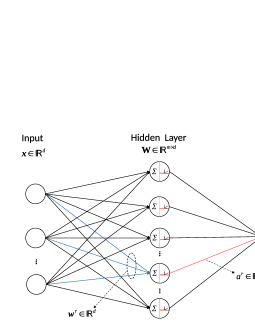
Figure 1: The architecture of the two-layer fully connected neural network with ReLU activation.

The details of the neural network. In this work, we consider a two-layer fully connected neural network $f:\mathbb{R}^{d}\to\mathbb{R}$ as follows:

$$f(\mathbf{W},\textbf{a};\mathbf{x})=\frac{1}{\sqrt{m}}\sum_{r=1}^{m}a^{r}\sigma(\langle\mathbf{w}^{r},\mathbf{x}\rangle),$$ (7)

where $\mathbf{x}\in\mathbb{R}^{d}$ denotes the input features, $\mathbf{W}=(\mathbf{w}^{1},\mathbf{w}^{2},\cdots,\mathbf{w}^{m})\in\mathbb{R}^{d\times m}$ denotes the weight matrix of the hidden layer, $\textbf{a}=(a^{1},a^{2},\cdots,a^{m})\in\mathbb{R}^{m}$ denotes the output weight vector and $\sigma(z)=z\cdot\mathbb{I}\{z\geq 0\}$ denotes the ReLU activation function. Figure 1 shows the architecture of the neural network. The parameters follow the random initialization scheme as $\mathbf{w}^{r}\sim\mathcal{N}(0,\textit{I}_{d})$ and $a^{r}\sim Rademacher(1/2)$ for any $r\in[m]$.

Following the settings in [16, 23, 20], we keep the output layer $\mathbf{a}$ fixed after initialization and only optimize the weight matrix $\mathbf{W}$ through minimizing the square loss

$${L}(\mathbf{W},\mathbf{a})=\frac{1}{2}\sum_{i=1}^{n}(y_{i}-f(\mathbf{W},\textbf{a};\mathbf{x}_{i}))^{2}.$$ (8)

Then the gradient for the weight vector of the $r$-th neuron can be calculated as:

$$\frac{\partial{L}(\mathbf{W},\mathbf{a})}{\partial\mathbf{w}^{r}}=\frac{1}{\sqrt{m}}\sum_{i=1}^{n}(f(\mathbf{W},\textbf{a};\mathbf{x}_{i})-y_{i})a^{r}\mathbf{x}_{i}\mathbb{I}\{{\langle\mathbf{w}^{r},\mathbf{x}_{i}\rangle\geq 0}\}.$$ (9)

Although this model is a simple two-layer neural network, its loss landscape is still non-convex and non-smooth due to the use of ReLU activation function. However, the objective function ${L}$ becomes convex when the weight matrix $\mathbf{W}$ is fixed and just optimizes the output layer $\mathbf{a}$, and this setting has been studied in [43].

Algorithm 1 Training Two-Layer Fully Connected ReLU Neural Network with NAG.

1:Parameters: learning rate $\eta>0$, momentum parameter $0\leq\beta<1$.

2:Initialization: $\mathbf{v}^{r}(0)=\mathbf{w}^{r}(0)\sim\mathcal{N}(0,I_{d})$, $a^{r}\sim Rademacher(1/2)$ for $r\in[m]$.

3:for $t=0,\ldots,T$ do

4:     for $r=1,\ldots,m$ do

5:         Calculate gradient $\frac{\partial{L}(\mathbf{w}(t),\mathbf{a})}{\partial\mathbf{w}^{r}(t)}$ for $\mathbf{w}^{r}$ using (9).

6:         Update $\mathbf{v}^{r}$: $\mathbf{v}^{r}(t+1)=\mathbf{w}^{r}(t)-\eta\frac{\partial{L}(\mathbf{w}(t),\mathbf{a})}{\partial\mathbf{w}^{r}(t)}$.

7:         Update $\mathbf{w}^{r}$: $\mathbf{w}^{r}(t+1)=\mathbf{v}^{r}(t+1)+\beta(\mathbf{v}^{r}(t+1)-\mathbf{v}^{r}(t))$.

8:     end for

9:end for

NTK theory. This theory was first introduced by Jacot [22] to study the optimization of infinite wide neural networks. It is closely related to a Gram matrix $\bm{H}_{t}$, which is defined as:

$$\bm{H}_{t}(\mathbf{x}_{i},\mathbf{x}_{j})=\langle\nabla_{\bm{\theta}}f(\bm{\theta}_{t};\mathbf{x}_{i}),\nabla_{\bm{\theta}}f(\bm{\theta}_{t};\mathbf{x}_{j})\rangle,\forall\;(i,j)\in[n]\times[n],$$ (10)

where $f$ is the neural network model and $\theta$ represents its parameter. Clearly, $\bm{H}_{t}$ is positive semi-definite due to the property of Gram matrix and varies according to $\theta_{t}$. As the width of the neural network goes to infinity, the limit matrix $\bar{\bm{H}}:=\lim_{m\to\infty}\bm{H}_{0}$ is determined by the initialization and architecture of the corresponding neural network $f$, which is the so-called NTK matrix. When the neural network is sufficiently over-parameterized, $\bm{\theta}_{t}$ barely changes from its initial $\bm{\theta}_{0}$, which in turn guarantees $\bm{H}_{t}$ stays close to $\bar{\bm{H}}$ during training [16, 22, 20]. As a result, the over-parameterized neural network behaves similarly to its linearization around $\bm{\theta}_{0}$.

Given the specific two-layer neural network (7) and the objective function (8), it has the corresponding $\bm{H}_{t}$ as:

$$\bm{H}_{t}(\mathbf{x}_{i},\mathbf{x}_{j})=\frac{1}{m}\sum_{r=1}^{m}\langle\mathbf{x}_{i},\mathbf{x}_{j}\rangle\mathbb{I}\{\langle\mathbf{w}_{t}^{r},\mathbf{x}_{i}\rangle\geq 0\&\langle\mathbf{w}_{t}^{r},\mathbf{x}_{j}\rangle\geq 0\},$$ (11)

and the NTK $\bar{\bm{H}}$ can be calculated with the expected value

$$\bar{\bm{H}}(\mathbf{x}_{i},\mathbf{x}_{j}) = \mathbb{E}_{\mathbf{w}\sim N(0,\textit{I})}[\langle\mathbf{x}_{i},\mathbf{x}_{j}\rangle\mathbb{I}\{\langle\mathbf{w},\mathbf{x}_{i}\rangle\geq 0\&\langle\mathbf{w},\mathbf{x}_{j}\rangle\geq 0\}]$$ (12)

$$= \langle\mathbf{x}_{i},\mathbf{x}_{j}\rangle\frac{\pi-arccos(\langle\mathbf{x}_{i},\mathbf{x}_{j}\rangle)}{2\pi}.$$

In addition, the above $\bar{\bm{H}}$ is strictly positive when the training dataset satisfies $\mathbf{x}_{i}\neq\mathbf{x}_{j}$ for all $i\neq j$ [16].

4 Main results

In this section, we analyze the dynamics of NAG’s residual error from a discrete view and give a non-asymptotic convergence rate with specific learning rate and momentum parameter, which is inspired by [16] and [23].

4.1 Intuition behind our proof

To start with, we intuitively illustrate the main idea of our proof under the infinite width assumption. As mentioned in Section 3.2, some theoretical and empirical works [44, 45] have shown that the outputs of the over-parameterized neural network can be approximated by its first-order Taylor expansion around its initial parameter as:

$$f(\bm{\theta};\mathbf{x})\approx f(\bm{\theta}_{0};\mathbf{x})+\langle\nabla f(\bm{\theta}_{0};\mathbf{x}),\bm{\theta}-\bm{\theta}_{0}\rangle.$$ (13)

By taking the derivative on both sides of (13), it has

$$\nabla_{\bm{\theta}}f(\bm{\theta};\mathbf{x})\approx\nabla_{\bm{\theta}}f(\bm{\theta}_{0};\mathbf{x}).$$ (14)

For simplicity, let $\mathcal{X}=(\mathbf{x}_{1},\cdots,\mathbf{x}_{n})\in\mathbb{R}^{d\times n}$ and $\mathcal{Y}=(y_{1},\cdots,y_{n})\in\mathbb{R}^{n}$ be the concatenation of the features and the corresponding labels of dataset $\mathcal{D}$. In addition, we define $f(\bm{\theta};\mathcal{X})=(f(\bm{\theta};\mathbf{x}_{1}),\cdots,f(\bm{\theta};\mathbf{x}_{n}))\in\mathbb{R}^{n}$,$\nabla_{\bm{\theta}}f(\bm{\theta};\mathcal{X})=(\nabla_{\bm{\theta}}f(\bm{\theta};\mathbf{x}_{1}),\cdots,\nabla_{\bm{\theta}}f(\bm{\theta};\mathbf{x}_{n}))^{\top}\in\mathbb{R}^{n\times k}$ and $\bm{\xi}=(f(\bm{\theta};\mathbf{x}_{1})-y_{1},\cdots,f(\bm{\theta};\mathbf{x}_{n})-y_{n})\in\mathbb{R}^{n}$ as the concatenated outputs, gradients and residual errors of the neural network, respectively. Plugging NAG’s update rule (6) into (13), it has

$$f(\bm{\theta}_{t+1};\mathcal{X})$$ (15)

$$\approx \!\!\!\!f(\bm{\theta}_{0};\mathcal{X})\!+\!\nabla_{\bm{\theta}}f(\bm{\theta}_{0};\mathcal{X})\big{(}\bm{\theta}_{t}\!-\!\eta\nabla_{\bm{\theta}}{L}(\bm{\theta}_{t})\!+\!\beta(\bm{\theta}_{t}\!-\!\bm{\theta}_{t\!-\!1})\!-\!\eta\beta\big{(}\nabla_{\bm{\theta}}{L}(\bm{\theta}_{t})\!-\!\nabla_{\bm{\theta}}{L}(\bm{\theta}_{t\!-\!1})\big{)}\!-\!\bm{\theta}_{0}\big{)}$$

$$\approx \!\!\!\!f(\bm{\theta}_{t};\mathcal{X})-\eta\beta\nabla_{\bm{\theta}}f(\bm{\theta}_{0};\mathcal{X})\big{(}\nabla_{\bm{\theta}}{L}(\bm{\theta}_{t})-\nabla_{\bm{\theta}}{L}(\bm{\theta}_{t-1})\big{)}\!-\!\eta\nabla_{\bm{\theta}}f(\bm{\theta}_{0};\mathcal{X})\nabla_{\bm{\theta}}{L}(\!\bm{\theta}_{t};\mathcal{X})$$

$$+ \!\!\!\!\beta\big{(}f(\bm{\theta}_{t};\mathcal{X})\!-\!f(\bm{\theta}_{t-1};\mathcal{X})\big{)},$$

where the last approximation uses (13). Expanding $\nabla_{\bm{\theta}}{L}(\bm{\theta}_{t})$ with (8), it has

$$\nabla_{\bm{\theta}}{L}(\bm{\theta}_{t})=\nabla_{\bm{\theta}}f(\bm{\theta}_{t};\mathcal{X})^{\top}(f(\bm{\theta}_{t};\mathcal{X})-\mathcal{Y}).$$ (16)

Then, plugging (14) and (16) into (15), it has the approximated residual error as:

$$\bm{\xi}_{t+1}\!\!\! = \!\!\!f(\bm{\theta}_{t+1};\mathcal{X})-\mathcal{Y}$$ (17)

$$\approx \!\!\!\!\!\bm{\xi}_{t}\!-\!\eta\bm{H}_{0}\bm{\xi}_{t}\!+\!\beta(\bm{\xi}_{t}\!-\!\bm{\xi}_{t-1})\!-\!\eta\beta\bm{H}_{0}(\bm{\xi}_{t}-\bm{\xi}_{t-1}).$$

Reformulating (17), it has

$$\begin{bmatrix}\bm{\xi}_{t+1}\\ \bm{\xi}_{t}\end{bmatrix}\approx\begin{bmatrix}(1\!+\!\beta)(\mathbf{I}_{n}\!-\!\eta\bm{H}_{0})\!&\!\beta(\!-\mathbf{I}_{n}\!+\!\eta\bm{H}_{0})\\ \mathbf{I}_{n}\!&\!\textbf{0}_{n}\end{bmatrix}\begin{bmatrix}\bm{\xi}_{t}\\ \bm{\xi}_{t-1}\end{bmatrix},$$ (18)

where $\mathbf{I}_{n}\in\mathbb{R}^{n\times n}$ and $\textbf{0}_{n}\in\mathbb{R}^{n\times n}$ denote the identity matrix and zero matrix, respectively. Similar to the quadratic convex optimization case [30, 46], the residual error in (18) follows a linear dynamical system. When the spectral norm of the coefficient matrix in (18) is less than one, the residual error decays to zero at an asymptotic linear convergence rate according to Gelfand’s formula [28]. However, this result is asymptotic and depends on the infinite width assumption. In contrast, we rely on a mild assumption about the width and provide a non-asymptotic convergence result.

4.2 Residual dynamics for NAG

Our analysis depends on an important event:

$$A_{ir}=\{\exists\mathbf{w}:\|\mathbf{w}-\mathbf{w}_{0}^{r}\|\leq R,\mathbb{I}\{\langle\mathbf{w},\mathbf{x}_{i}\rangle\}\neq\mathbb{I}\{\langle\mathbf{w}_{0}^{r},\mathbf{x}_{i}\rangle\}\},$$

where $R>0$ is a constant. This event describes whether there exists a weight vector that restricts in a neighbourhood of its initial but has a different activation pattern compared to the initial for the same input. Here, the activation pattern is defined as the output of $\mathbb{I}\{\langle\mathbf{w},\mathbf{x}\rangle\}$. Then one can define the set $S_{i}=\{r\in[m]:\mathbb{I}\{A_{ir}\}=0\}$ and its complementary set $S_{i}^{\perp}=[m]\setminus S_{i}$ to separate the neurons with two parts.

By utilizing the intuition introduced in Section 4.1, we provide the recursion formulation of the residual error for a finite width two-layer neural network trained by NAG.

Lemma 1.

Let $\bm{\xi}_{t}$ be the residual error vector of the $t$-th iterate in NAG for any $t\in[T]$, it has

$${{\bm{\xi}_{t+1}=\bm{\xi}_{t}-\eta\bm{H}_{0}\bm{\xi}_{t}+\beta(\bm{\xi}_{t}-\bm{\xi}_{t-1})-\eta\beta\bm{H}_{0}(\bm{\xi}_{t}-\bm{\xi}_{t-1})+\bm{\psi}_{t}+\bm{\phi}_{t}}},$$ (19)

where

$$\bm{\psi}_{t}=\beta\eta(\bm{H}_{t-1}-\bm{H}_{0})\bm{\xi}_{t-1}-(1+\beta)\eta(\bm{H}_{t}-\bm{H}_{0})\bm{\xi}_{t},$$ (20)

and the $i$-th element of $\bm{\phi}_{t}$ is bounded by

$$|\bm{\phi}_{t}[i]|\leq\frac{\sup_{j\in[n]}|S_{j}^{\perp}|\sqrt{n}\eta}{m}\left[(2+4\beta)\|\bm{\xi}_{t}\|+3\beta\|\bm{\xi}_{t-1}\|+2\sum_{i=0}^{t-1}\beta^{t+1-i}\|\bm{\xi}_{i}\|\right].$$ (21)

The proof of Lemma 1 can be found in A. Denotes $\mathbf{z}_{t}=[\bm{\xi}_{t};\bm{\xi}_{t-1}]$ as the augmented residual error at iteration $t$, then (19) can be reformulated as:

$$\mathbf{z}_{t+1}=\mathbf{M}\mathbf{z}_{t}+\bm{\mu}_{t},$$ (22)

where $\bm{\mu}_{t}=[\bm{\psi}_{t}+\bm{\phi}_{t};\textbf{0}]$ and the coefficient matrix $\mathbf{M}=\begin{bmatrix}(1\!+\!\beta)(\mathbf{I}_{n}\!-\!\eta\bm{H}_{0})\!&\!\beta(\!-\mathbf{I}_{n}\!+\!\eta\bm{H}_{0})\\ \mathbf{I}_{n}\!&\!\textbf{0}_{n}\end{bmatrix}$.

Note that, compared to the linear dynamical system (18), the finite width one has an additional term $\bm{\mu}$, which can be regarded as a perturbation and we will discuss its bound later. Furthermore, as shown in [23], HB has the residual dynamics as

$$\begin{bmatrix}\bm{\xi}_{t+1}\\ \bm{\xi}_{t}\end{bmatrix}=\begin{bmatrix}(1\!+\!\beta)\mathbf{I}_{n}\!-\!\eta\bm{H}_{0}\!&\!-\beta\bm{H}_{0})\\ \mathbf{I}_{n}\!&\!\textbf{0}_{n}\end{bmatrix}\begin{bmatrix}\bm{\xi}_{t}\\ \bm{\xi}_{t-1}\end{bmatrix}+\bm{\mu}_{t}^{{}^{\prime}},$$ (23)

which differs from (22) both in the coefficient matrix and perturbation term.

4.3 Convergence analysis

Table 1: Summary of the Convergence Results. Let $m$ denotes the width of neural network. Let $n$ denotes the number of input data points. Let $\delta$ denotes the failure probability. Let $t$ denotes the iteration number. Define $\lambda=\lambda_{min}(\bar{\bm{H}})$ , $\lambda_{max}=\lambda_{max}(\bar{\bm{H}})+\lambda/4$ and $\kappa=4\kappa(\bar{\bm{H}})/3+1/3$.

Method	Width of the Neural Network	Hyperparameter Choice	Convergence Rate
GD [25]	$\Omega(\lambda^{-4}\delta^{-3}n^{6})$	$\eta=\Theta(\frac{1}{\lambda_{max}(\bar{\bm{H}})})$	$(1-\Theta(\frac{1}{\kappa}))^{t}$
HB [23]	$\Omega(\lambda^{-2}n^{4}\kappa^{2}\log^{3}(n/\delta))$	$\eta=\frac{1}{\lambda_{max}},\beta=(1-\frac{1}{2\sqrt{\kappa}})^{2}$	$(1-\frac{1}{4\sqrt{\kappa}})^{t}$
NAG	$\Omega(\lambda^{-2}n^{4}\kappa^{2}\log^{3}(n/\delta))$	$\eta=\frac{1}{2\lambda_{max}},\beta=\frac{3\sqrt{\kappa}-2}{3\sqrt{\kappa}+2}$	$(1-\frac{1}{2\sqrt{\kappa}})^{t}$

By recursively using (22), it has

$$\mathbf{z}_{t}=\mathbf{M}^{t}\mathbf{z}_{0}+\sum_{i=0}^{t-1}\mathbf{M}^{t-1-i}\bm{\mu}_{i}.$$ (24)

Then applying Cauchy-Schwarz inequality on (24), we have

$$\|\mathbf{z}_{t}\|\leq\|\mathbf{M}^{t}\mathbf{z}_{0}\|+\|\sum_{i=0}^{t-1}\mathbf{M}^{t-1-i}\bm{\mu}_{i}\|.$$ (25)

In order to prove the convergence of NAG, it needs to separately derive bounds for the two terms on the right-hand side of (25). The first term is the norm of the product between the matrix power $\mathbf{M}^{t}$ and the vector $\mathbf{z}_{0}$. We provide its upper bound in the following lemma.

Lemma 2.

Assume $\bm{H}\in\mathbb{R}^{n\times n}$ is a symmetry positive definite matrix. Let $\mathbf{M}=\begin{bmatrix}(1\!+\!\beta)(\mathbf{I}_{n}\!-\!\eta\bm{H})&\beta(-\mathbf{I}_{n}\!+\!\eta\bm{H})\\ \mathbf{I}_{n}&\textbf{0}_{n}\end{bmatrix}\in\mathbb{R}^{2n\times 2n}$. Suppose a sequence of iterates $\{\mathbf{v}_{i}\}$ satisfy $\mathbf{v}_{t}=\mathbf{M}\mathbf{v}_{t-1}$ for any $t\leq T$. If $\beta$ and $\eta$ are chosen that satisfy $1>\beta\geq\frac{1-\sqrt{\eta\lambda_{min}(\bm{H})}}{1+\sqrt{\eta\lambda_{min}(\bm{H})}}$ and $0<\eta\leq 1/\lambda_{max}(\bm{H})$, then it has the bound at any iteration $k\leq T$ as

$$\|\mathbf{v}_{k}\|\leq C\big{(}\sqrt{\beta(1-\eta\lambda_{min}(\bm{H}))}\big{)}^{k}\|\mathbf{v}_{0}\|,$$ (26)

where $C=\frac{2\beta(1-\eta\lambda_{min}(\bm{H}))+2}{\sqrt{\min\{g(\beta,\eta\lambda_{min}(\bm{H})),g(\beta,\eta\lambda_{max}(\bm{H}))\}}}$ and the function $g$ is defined as $g(x,y)=4x(1-y)-[(1+x)(1-y)]^{2}$.

The proof is provided in the B. Given the ranges of the hyperparameters $\eta$ and $\beta$, it is easy to observe that $\sqrt{\beta(1-\eta\lambda_{min}(H))}<1$, which ensures the decline of $\|\mathbf{v}_{k}\|$ during evolution. For further determining the upper bounds for C and the decay rate, we set $\eta$ and $\beta$ with the spectrum of $\bm{H}$.

Lemma 3.

Assume $0<\lambda\leq\lambda_{min}(\bm{H})\leq\lambda_{max}(\bm{H})\leq\lambda_{max}$. Denote ${\kappa}=\lambda_{max}/\lambda$. With $\eta=1/2\lambda_{max}$ and $\beta=\frac{3\sqrt{{\kappa}}-2}{3\sqrt{{\kappa}}+2}$, it has

$$\sqrt{\beta(1-\eta\lambda_{min}(\bm{H}))}\leq 1-\frac{2}{3\sqrt{{\kappa}}},\;\;C\leq 12\sqrt{{\kappa}}.$$ (27)

Furthermore, it should be noted that $\mathbf{M}$ in (25) is composed by $\bm{H}_{0}$, which depends on the random initialization of $\mathbf{W}_{0}$. For an over-parameterized neural network, the eigenvalues of the random matrix $\bm{H}_{0}$ can be bounded by the spectrum of the deterministic NTK matrix $\bar{\bm{H}}$ [23], thereby allowing us to determine the hyperparameters with specific values.

Lemma 4.

(Lemma 13 in [23]) Denote $\lambda=\lambda_{min}(\bar{\bm{H}})$. Set $m=\Omega(\lambda^{-2}n^{2}\log(n/\delta))$. Assume $\mathbf{w}_{0}^{r}\sim\mathcal{N}(0,I_{d})$ for all $r\in[n]$. With probability at least $1-\delta$, it holds that

$$\|\bm{H}_{0}-\bar{\bm{H}}\|_{F}\leq\frac{\lambda}{4} \lambda_{min}(\bm{H}_{0})\geq\frac{3}{4}\lambda>0\;\;\;\;\lambda_{max}(\bm{H}_{0})\leq\lambda_{max}(\bar{\bm{H}})+\frac{\lambda}{4}.$$ ,

As a result, the condition number of $\bm{H}_{0}$ is bounded by

$$\kappa(\bm{H}_{0})\leq\frac{4}{3}\kappa(\bar{\bm{H}})+\frac{1}{3}.$$ (28)

Now we turn to analyzing the second term on the right-hand side of (25), which is also composed by the product of the matrix power $\mathbf{M}^{i}$ and a bounded vector. Then it only needs to bound the norm of $\bm{\mu}$. Using the Cauchy-Schwarz inequality, it has $\|\bm{\mu}_{t}\|\leq\|\bm{\phi}_{t}\|+\|\bm{\psi}_{t}\|$.

From (21), we observe that the bound of $|\bm{\phi}_{t}[i]|$ mainly depends on the term $|S_{i}^{\perp}|$, which describes how many neurons change their activation patterns on the $i$-th instance during training. According to recent studies [16, 21], $|S_{i}^{\perp}|$ has an upper bound $4mR$, which is determined by the distance $R$ between $\mathbf{w}^{r}_{t}$ and its initialization for any $r\in[m]$ and $t\in[T]$. In D, Lemma 5 presents the details. When $R$ is small enough, it has $|S_{i}^{\perp}|\ll m$.

On the other hand, the bound of $\|\bm{\psi}_{t}\|$ is closely related to the distance between $\bm{H}_{t}$ and $\bm{H}_{0}$. Previous works [16, 21] showed that the upper bound of $\|\bm{H}_{t}-\bm{H}_{0}\|$ is also determined by the distance $R$, where Lemma 6 in D gives the details.

In Theorem 1, we derive $R=\mathcal{O}(1/\sqrt{m})$, which helps control the size of $\|\bm{\phi}_{t}\|$ and $\|\bm{\psi}_{t}\|$ with an appropriate $m$. The corresponding bounds for $R$, $\|\bm{\phi}\|$ and $\|\bm{\psi}\|$ are given in the proof of Theorem 1. Finally, we introduce our main result on the convergence of NAG.

Theorem 1.

Define $\lambda=\frac{3\lambda_{min}(\bar{\bm{H}})}{4}$, $\lambda_{max}=\lambda_{max}(\bar{\bm{H}})+\frac{\lambda}{4}$ and ${\kappa}=\frac{4}{3}\kappa(\bar{\bm{H}})+\frac{1}{3}$. Assume $\mathbf{w}_{0}^{r}\sim N(0,I_{d})$ and $a^{r}\sim Rademacher(1/2)$ for all $r\in[m]$. Suppose the number of the nodes in the hidden layer is $m=\Omega(\lambda^{-2}n^{4}\kappa^{2}log^{3}(n/\delta))$. If the leaning rate $\eta=1/(2\lambda_{max})$ and the momentum parameter $\beta=\frac{3\sqrt{{\kappa}}-2}{3\sqrt{{\kappa}}+2}$, with probability at least $1-\delta$ over the random initialization, the residual error for NAG at any iteration $t$ satisfies

$$\left\|\begin{bmatrix}\bm{\xi}_{t}\\ \bm{\xi}_{t-1}\end{bmatrix}\right\|\leq{(1-\frac{1}{2\sqrt{{\kappa}}})^{t}}2\gamma\textstyle\left\|\begin{bmatrix}\bm{\xi}_{0}\\ \bm{\xi}_{-1}\end{bmatrix}\right\|,$$ (29)

where $\gamma=12\sqrt{{\kappa}}$.

For every $r\in[m]$, we have

$$\|\mathbf{w}_{t}^{r}-\mathbf{w}_{0}^{r}\|\leq\frac{48\sqrt{2n\kappa}}{\lambda\sqrt{m}}\|\bm{\xi}_{0}\|.$$ (30)

Remark 1. With the initialization $\mathbf{W}_{-1}=\mathbf{W}_{0}$, it has $\bm{\xi}_{-1}=\bm{\xi}_{0}$. Thus, according to Theorem 1, the training error $\bm{\xi}_{t}$ of NAG converges linearly to zero at a $(1-\frac{1}{2\sqrt{\kappa}})^{t}$ rate after $t$ iteration, which indicates NAG is able to achieve the global minimum as GD and HB.

Remark 2. As shown in [16], GD converges at a rate $(1-{\frac{\eta\lambda}{2}})^{t}$, but with a small learning rate $\eta=\mathcal{O}(\frac{\lambda}{n^{2}})$. [25] further improved the bound of the learning rate to $\mathcal{O}(\frac{1}{\|{\bar{\bm{H}}}\|})$, where $\|{\bar{\bm{H}}}\|\leq n$ and provides an $\mathcal{O}(\lambda/n)$ improvement. This results in a faster convergence rate $(1-\Theta(1/\kappa))^{t}$ for GD. As shown in Theorem 1, NAG obtains a smaller convergence rate $(1-\Theta(1/\sqrt{\kappa}))^{t}$, which validates its acceleration over GD. Moreover, compard to the convergence rate of HB as proved in [23], our results show that NAG obtains a comparable convergence rate.

Remark 3. The initial residual error satisfies $\|\bm{\xi}_{0}\|^{2}=\mathcal{O}(nlog(m/\delta)log^{2}(n/\delta))$ as shown in Lemma 7. Therefore, the upper bound $R$ of $\|\mathbf{w}_{t}^{r}-\mathbf{w}_{0}^{r}\|$ scales as $\mathcal{O}(1/\sqrt{m})$ for any $r\in[m]$ according to (30). This is consistent with the NTK regime that the parameter is hardly changed when the neural network is over-parameterized. Moreover, the number of the changed activation patterns is bounded by $|S_{i}^{\perp}|=|\sum_{r=1}^{m}\mathbb{I}\{\langle\mathbf{w}_{t}^{r},\mathbf{x}_{i}\rangle\}\neq\mathbb{I}\{\langle\mathbf{w}_{0}^{r},\mathbf{x}_{i}\rangle\}|\leq 4mR$ according to Lemma 5. As a result, $\sum_{i\in[n]}|S_{i}^{\perp}|/(mn)$ can be upper bounded with $4R$, which also scales with $\mathcal{O}(1/\sqrt{m})$. On the other hand, GD has $R=\mathcal{O}(\frac{\sqrt{n}}{\lambda\sqrt{m}}\|\bm{\xi}_{0}\|)$ according to [16], which is smaller than NAG due to $\kappa>1$. Furthermore, $R$ of HB scales as $\mathcal{O}(\frac{\sqrt{n\kappa}}{\lambda\sqrt{m}}\|\bm{\xi}_{0}\|)$ [23], which is similar as NAG.

5 Numerical experiments

In this section, we conduct extensive experiments to validate our theoretical results, including i) the convergence comparison between NAG, HB and GD. ii) the impact of the over-parameterization on some quantities as introduced in Remark 3.

5.1 Setup

Six benchmark datasets are used in the experiments: FMNIST [47], MNIST [48], CIFAR10 [49] and three UCI regression datasets (ENERGY, HOUSING and YACHT) [50]. The pre-processing of the first three image classification datasets follows the procedures outlined in [20], where we use the first two classes of images with 10,000 training instances, where the label of the first class is set to +1 and -1 otherwise. For all six datasets, we normalize all instances with the unit norm.

According to Table 1, the eigenvalues of the NTK matrix $\bar{\bm{H}}$ are used to determine the hyperparameters of each optimizer. Note that the matrix $\bar{\bm{H}}$ is analytic, so its eigenvalues can be easily calculated based on (12). As described in Section 3.2, we use the same architecture and the initialization scheme of the neural network, which is trained with the square loss (8) in the deterministic setting. All experiments are conducted on 8 NVIDIA Tesla A100 GPU and the code is written in JAX [51].

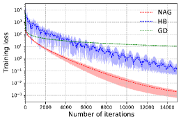
(a) FMNIST

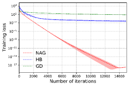
(b) MNIST

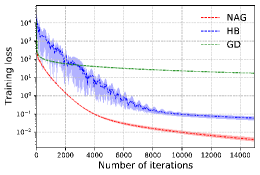
(c) CIFAR10

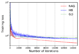
(d) ENERGY

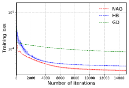
(e) HOUSING

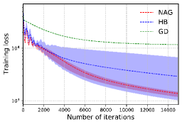
(f) YACHT

Figure 2: Convergence comparison among GD, HB and NAG.

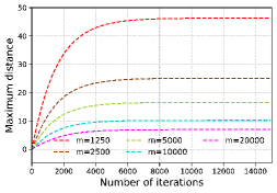
(a) FMNIST

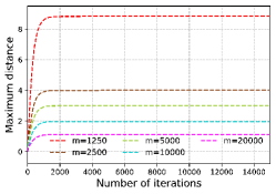
(b) MNIST

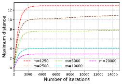
(c) CIFAR10

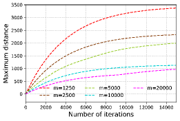
(d) ENERGY

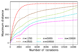
(e) HOUSING

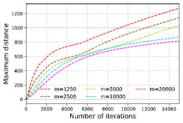
(f) YACHT

Figure 3: Maximum distance from initialization comparison for NAG with different width $m$.

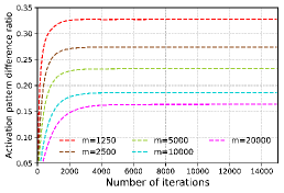
(a) FMNIST

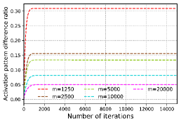
(b) MNIST

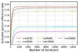
(c) CIFAR10

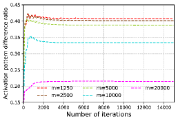
(d) ENERGY

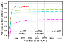
(e) HOUSING

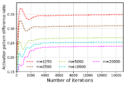
(f) YACHT

Figure 4: Activation pattern difference ratio comparison for NAG with different width $m$.

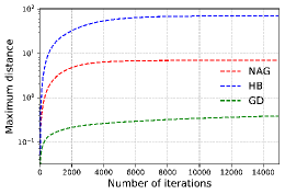
(a) FMNIST

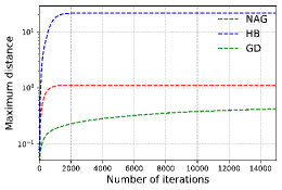
(b) MNIST

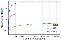
(c) CIFAR10

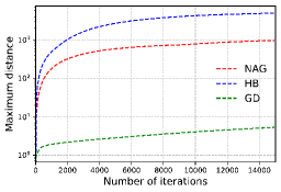
(d) ENERGY

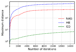
(e) HOUSING

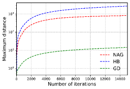
(f) YACHT

Figure 5: Maximum distance from initialization comparison among GD, HB and NAG with width $m=20000$.

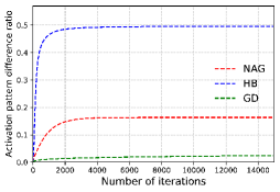
(a) FMNIST

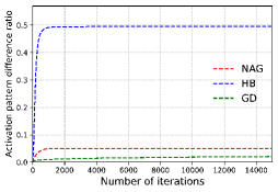
(b) MNIST

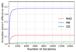
(c) CIFAR10

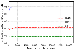
(d) ENERGY

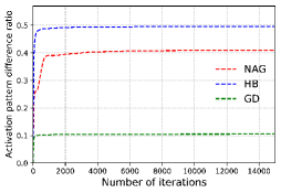
(e) HOUSING

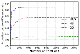
(f) YACHT

Figure 6: Activation pattern difference ratio comparison among GD, HB and NAG with width $m=20000$.

5.2 Results analysis

Convergence analysis. We first provide the convergence comparison among NAG, HB and GD. The neural network is trained with 5 different initialization seed for each dataset, and the width of the hidden layer is $20000$. The dashed line represents the mean training loss, while the shaded region represents the range of the maximum and minimum performance. From Fig 2, we observe that NAG converges faster than GD on all six datasets. Furthermore, it is noted that NAG achieves a comparable and even improved performance than HB. This is in accordance with our theoretical findings.

Impact of the over-parameterization. Secondly, we evaluate the impact of the over-parameterization on two quantities relevant to our theoretical analysis. One is the maximum distance $\max_{r\in[m]}\|\mathbf{w}_{t}^{r}-\mathbf{w}_{0}^{r}\|_{2}$, which is used to demonstrate the change of the parameter with respect to its initial [16]. The other is the activation pattern difference ratio $\frac{\sum_{i=1}^{n}\sum_{r=1}^{m}\mathbb{I}\{\mathbb{I}\{\langle\mathbf{w}_{t}^{r},\mathbf{x}_{i}\rangle\}\neq\mathbb{I}\{\langle\mathbf{w}_{0}^{r},\mathbf{x}_{i}\rangle\}\}}{mn}$. It describes the percentiles of pattern changes among $mn$ patterns [16, 23]. In Remark 3, we theoretically show the the upper bounds of these two quantities are all scaled as $\mathcal{O}(1/\sqrt{m})$, indicating that the parameter stays closer to its initial as the width increases. To observe the impact of the over-parameterization, we set the range of the width as $m\in[1250,2500,5000,10000,20000]$. Each neural network of different width is trained with 5 different initialization seed, where the solid line indicates the corresponding mean value. As shown in Fig 3 and Fig 4, the maximum distance and the activation pattern difference ratio both decrease as the width increases.

Moreover, we compare the above two quantities among NAG, HB and GD. From Remark 3, we show that the upper bound of the maximum distance from the initialization for NAG is larger than that of GD by a factor $\mathcal{O}(\sqrt{\kappa})$, resulting in a larger activation pattern difference ratio for NAG over GD. On the other hand, in Remark 3, we also show that NAG has comparable upper bounds for these two quantities as HB. We conduct the experiments in the same setting as the convergence analysis. According to Fig 5 and Fig 6, the two quantities of NAG are larger than that of GD. Comparing to HB, NAG obtains a comparable or smaller values. These phenomena support our theoretical results.

6 Conclusion and future work

In this paper, we focus on analyzing the training trajectory of NAG for optimizing a two-layer fully connected neural network with ReLU activation. By exploiting the connection between the NTK and the finite over-parametrized neural network, we show that NAG can achieve a non-asymptotic linear convergence rate to a global optimum. In the discrete-time scenario, our result provides theoretical guarantees for the acceleration of NAG over GD. In addition, our result implies NAG obtains a comparable convergence rate as HB.

An important future work is to extend our analysis to deep neural networks with different architectures (e.g., convolutional neural networks, graph neural networks, etc.) and activation functions (e.g., sigmoid, tanh, etc.). Recently, there are plenty of works studied the convergence of GD on different types of over-paramterized neural networks [18, 39, 37]. The key technical challenge lies in deriving and analyzing the associated residual dynamics, which might be complex due to the structure of the neural network. Meanwhile, in practice, many applications requires numerous entities, yet their interactions are highly incomplete. Currently, the latent factor model has attracted a lot of attention as a way to deal with this problem [52, 53, 54, 55]. It brings an interesting future direction for studying the acceleration of NAG for these problems, where the induced dynamics can be investigated using our approach.

Appendix A Proof of Lemma 1

Proof.

At iteration $t+1$, the output of the two-layer fully connected neural network for arbitrary feature $\mathbf{x}_{i}$ can be divided into two parts w.r.t the set $S_{i}$

$$f(\mathbf{W}_{t+1},\mathbf{a};\mathbf{x}_{i})$$ (31)

$$= \frac{1}{\sqrt{m}}\sum_{r=1}^{m}a^{r}\sigma(\langle\mathbf{w}_{t+1}^{r},\mathbf{x}_{i}\rangle)$$

$$= \!\!\!\frac{1}{\sqrt{m}}\sum_{r\in S_{i}}a^{r}\sigma(\langle\mathbf{w}_{t+1}^{r},\mathbf{x}_{i}\rangle)\!+\!\frac{1}{\sqrt{m}}\sum_{r\in S_{i}^{\perp}}a^{r}\sigma(\langle\mathbf{w}_{t+1}^{r},\mathbf{x}_{i}\rangle).$$

For brevity, we define $\mathbb{I}_{r,i}(t)=\mathbb{I}\{{\langle\mathbf{w}_{t}^{r},\mathbf{x}_{i}\rangle\!\geq\!0}\}$ and use $\frac{\partial{L}}{\partial\mathbf{w}_{t}^{r}}$ instead of $\frac{\partial{L}(\mathbf{W}_{t},\mathbf{a})}{\partial\mathbf{w}_{t}^{r}}$. Based on the updating scheme (6), the first part of  (31) can be decomposed as:

$$\frac{1}{\sqrt{m}}\sum_{r\in S_{i}}a^{r}\sigma(\langle\mathbf{w}_{t+1}^{r},\mathbf{x}_{i}\rangle)$$ (32)

$${=} \frac{1}{\sqrt{m}}\sum_{r\in S_{i}}a^{r}\sigma(\langle\mathbf{w}_{t}^{r}-\eta\frac{\partial{L}}{\partial\mathbf{w}_{t}^{r}}+\beta(\mathbf{w}_{t}^{r}-\mathbf{w}_{t-1}^{r})-\beta\eta(\frac{\partial{L}}{\partial\mathbf{w}_{t}^{r}}-\frac{\partial{L}}{\partial\mathbf{w}_{t-1}^{r}}),\mathbf{x}_{i}\rangle)$$

$$\overset{\text{a}}{=} \frac{1}{\sqrt{m}}\!\sum_{r\in S_{i}}\!a^{r}\langle\mathbf{w}_{t}^{r}-\eta\frac{\partial{L}}{\partial\mathbf{w}_{t}^{r}}+\beta(\mathbf{w}_{t}^{r}-\mathbf{w}_{t-1}^{r})-\beta\eta(\frac{\partial{L}}{\partial\mathbf{w}_{t}^{r}}-\frac{\partial{L}}{\partial\mathbf{w}_{t-1}^{r}}),\mathbf{x}_{i}\rangle\mathbb{I}_{r,i}(t+1)$$

$$\overset{\text{b}}{=} \!\!\!\!\!\!{{\frac{1\!+\!\beta}{\sqrt{m}}\!\!\sum_{r\in S_{i}}\!a^{r}\langle\mathbf{w}_{t}^{r},\mathbf{x}_{i}\rangle\mathbb{I}_{r,i}(t)\!-\!\frac{\beta}{\sqrt{m}}\!\!\sum_{r\in S_{i}}\!a^{r}\langle\mathbf{w}_{t\!-\!1}^{r},\mathbf{x}_{i}\rangle\mathbb{I}_{r,i}(t\!-\!1)}}\!+\!\frac{\eta\beta}{\sqrt{m}}\!\!\sum_{r\in S_{i}}\!\!a^{r}\!\langle\frac{\partial{L}}{\partial\mathbf{w}_{t\!-\!1}^{r}},\mathbf{x}_{i}\rangle\mathbb{I}_{r,i}(t\!\!-\!\!1)$$

$$- \!\!\!\!\!\!\frac{(1\!+\!\beta)\eta}{\sqrt{m}}\!\!\sum_{r\in S_{i}}\!\!a^{r}\langle\frac{\partial{L}}{\partial\mathbf{w}_{t}^{r}},\mathbf{x}_{i}\rangle\mathbb{I}_{r,i}(t)$$

$$\overset{\text{c}}{=} \!\!\!\!\!\!(1+\beta)f(\mathbf{W}_{t},\mathbf{a};\mathbf{x}_{i})-\frac{1+\beta}{\sqrt{m}}\sum_{r\in S_{i}^{\perp}}a^{r}\langle\mathbf{w}_{t}^{r},\mathbf{x}_{i}\rangle\mathbb{I}_{r,i}(t)-\beta f(\mathbf{W}_{t-1},\mathbf{a};\mathbf{x}_{i})$$

$$+ \!\!\!\!\!\frac{\beta}{\sqrt{m}}\!\sum_{r\in S_{i}^{\perp}}a^{r}\langle\mathbf{w}_{t-1}^{r},\mathbf{x}_{i}\rangle\mathbb{I}_{r,i}(t-1)\!-\!(1+\beta)\eta\sum_{j=1}^{n}\bm{\xi}_{t}[j]\bm{H}_{t}[i,j]\!+\!\beta\eta\sum_{j=1}^{n}\bm{\xi}_{t-1}[j]\bm{H}_{t-1}[i,j]$$

$$+ \!\!\!\!\!\!\frac{(1+\beta)\eta}{m}\!\!\sum_{j=1}^{n}\mathbf{x}_{i}^{\top}\mathbf{x}_{j}\bm{\xi}_{t}[j]\!\!\sum_{r\in S_{i}^{\perp}}\!\mathbb{I}_{r,i}(t)\mathbb{I}_{r,j}(t)\!-\!\frac{\beta\eta}{m}\!\!\sum_{j=1}^{n}\mathbf{x}_{i}^{\top}\mathbf{x}_{j}\bm{\xi}_{t-1}[j]\!\!\sum_{r\in S_{i}^{\perp}}\!\mathbb{I}_{r,i}(t\!-\!1)\mathbb{I}_{r,i}(t\!-\!1),$$

where (a) applies the property of ReLU activation $\sigma(x)=x\mathbb{I}\{x\geq 0\}$,
(b) exploits the the neurons of the set $S_{i}$ always keep the sign of their activation pattern,
(c) uses the expansion of the subgradient (9) and the Gram matrix $\bm{H}_{t}$ (11).

With (32), the $i$-th element of the residual error can be decomposed as:

$$\bm{\xi}_{t+1}[i]$$

$$= f(\mathbf{W}_{t+1},\mathbf{a};\mathbf{x}_{i})-y_{i}$$

$$= \!\!\!\!\frac{1}{\sqrt{m}}\!\!\sum_{r\in S_{i}}\!\!a^{r}\sigma(\langle\mathbf{w}_{t+1}^{r},\mathbf{x}_{i}\rangle)\!+\!\frac{1}{\sqrt{m}}\!\!\sum_{r\in S_{i}^{\perp}}\!\!a^{r}\sigma(\langle\mathbf{w}_{t+1}^{r},\mathbf{x}_{i}\rangle)\!-\!y_{i}$$

$$= \bm{\xi}_{t}[i]+\beta(\bm{\xi}_{t}[i]-\bm{\xi}_{t-1}[i])-(1+\beta)\eta\sum_{j=1}^{n}\bm{H}_{0}[i,j]\bm{\xi}_{t}[j]+\beta\eta\!\!\sum_{j=1}^{n}\!\!\bm{H}_{0}[i,j]\bm{\xi}_{t-1}[j]$$

$$+ \beta\eta\!\!\sum_{j=1}^{n}(\bm{H}_{t-1}[i,j]\!-\!\bm{H}_{0}[i,j])\bm{\xi}_{t-1}[j]-(1+\beta)\eta\!\!\sum_{j=1}^{n}(\bm{H}_{t}[i,j]\!\!-\!\!\bm{H}_{0}[i,j])\bm{\xi}_{t}[j]$$

$$+ \!\!\frac{(1\!\!+\!\!\beta)\eta}{m}\!\!\sum_{j=1}^{n}\!\!\mathbf{x}_{i}^{\top}\mathbf{x}_{j}\bm{\xi}_{t}[j]\!\!\sum_{r\in S_{i}^{\perp}}\!\!\mathbb{I}_{r,i}(t)\mathbb{I}_{r,j}(t)-\frac{\beta\eta}{m}\!\!\sum_{j=1}^{n}\!\!\mathbf{x}_{i}^{\top}\mathbf{x}_{j}\bm{\xi}_{t-1}[j]\!\!\sum_{r\in S_{i}^{\perp}}\!\!\mathbb{I}_{r,i}(t-1)\mathbb{I}_{r,j}(t-1)$$

$$+ \!\!\!\!\frac{1}{\sqrt{m}}\!\!\!\sum_{r\in S_{i}^{\perp}}\!\!a^{r}\sigma(\langle\mathbf{w}_{t+1}^{r},\mathbf{x}_{i}\rangle)-a^{r}\sigma(\langle\mathbf{w}_{t}^{r},\mathbf{x}_{i}\rangle)-\frac{\beta}{\sqrt{m}}\!\!\sum_{r\in S_{i}^{\perp}}\!\!a^{r}\sigma(\langle\mathbf{w}_{t}^{r},\mathbf{x}_{i}\rangle)-a^{r}\sigma(\langle\mathbf{w}_{t-1}^{r},\mathbf{x}_{i}\rangle)$$

In words, the residual error on the whole training dataset can be written in a recursive form as:

$$\bm{\xi}_{t+1} = \bm{\xi}_{t}+\beta(\bm{\xi}_{t}-\bm{\xi}_{t-1})-(1+\beta)\eta\bm{H}_{0}\bm{\xi}_{t}+\beta\eta\bm{H}_{0}\bm{\xi}_{t-1}+\bm{\psi}_{t}+\bm{\phi}_{t}$$

where $\bm{\psi}_{t}=\beta\eta(\bm{H}_{t-1}-\bm{H}_{0})\bm{\xi}_{t-1}-(1+\beta)\eta(\bm{H}_{t}-\bm{H}_{0})\bm{\xi}_{t}$ and the i-th element of $\bm{\phi}_{t}$ have the following form

$$\bm{\phi}_{t}[i]\!\!\!\! = \!\!\!\!\frac{(1\!\!+\!\!\beta)\eta}{m}\!\!\sum_{j=1}^{n}\!\!\mathbf{x}_{i}^{\top}\mathbf{x}_{j}\bm{\xi}_{t}[j]\!\!\sum_{r\in S_{i}^{\perp}}\!\!\mathbb{I}_{r,i}(t)\mathbb{I}_{r,j}(t)-\frac{\beta\eta}{m}\!\!\sum_{j=1}^{n}\!\!\mathbf{x}_{i}^{\top}\mathbf{x}_{j}\bm{\xi}_{t-1}[j]\!\!\!\sum_{r\in S_{i}^{\perp}}\!\!\mathbb{I}_{r,i}(t-1)\mathbb{I}_{r,j}(t-1)$$

$$+ \!\!\!\!\frac{1}{\sqrt{m}}\!\!\sum_{r\in S_{i}^{\perp}}\!\!a^{r}\sigma(\langle\mathbf{w}_{t+1}^{r},\mathbf{x}_{i}\rangle)\!-\!a^{r}\sigma(\langle\mathbf{w}_{t}^{r},\mathbf{x}_{i}\rangle)\!-\!\frac{\beta}{\sqrt{m}}\!\!\sum_{r\in S_{i}^{\perp}}\!\!a^{r}\sigma(\langle\mathbf{w}_{t}^{r},\mathbf{x}_{i}\rangle)\!-\!a^{r}\sigma(\langle\mathbf{w}_{t-1}^{r},\mathbf{x}_{i}\rangle).$$

In addition, it has $\sum_{r\in S_{i}^{\perp}}\mathbb{I}_{r,i}(t)\mathbb{I}_{r,j}(t)\leq|S_{i}^{\perp}|$. Using $\|\mathbf{x}_{i}\|\leq 1$ and 1-Lipschitz property of ReLU activation $\sigma(\cdot)$, it has

$$a^{r}\big{[}\sigma(\langle\mathbf{w}_{t+1}^{r},\mathbf{x}_{i}\rangle)-\sigma(\langle\mathbf{w}_{t}^{r},\mathbf{x}_{i}\rangle)\big{]} \leq |a^{r}\big{[}\sigma(\langle\mathbf{w}_{t+1}^{r},\mathbf{x}_{i}\rangle)-\sigma(\langle\mathbf{w}_{t}^{r},\mathbf{x}_{i}\rangle)\big{]}|$$

$$\leq |\langle\mathbf{w}_{t+1}^{r}-\mathbf{w}_{t}^{r},\mathbf{x}_{i}\rangle|$$

$$\leq \|\mathbf{w}_{t+1}^{r}-\mathbf{w}_{t}^{r}\|\|\mathbf{x}_{i}\|$$

$$\leq \|\mathbf{w}_{t+1}^{r}-\mathbf{w}_{t}^{r}\|.$$

Therefore, we have

$$|\bm{\phi}_{t}[i]|$$

$${\leq} \!\!\!\!\frac{(1+\beta)\eta|S_{i}^{\perp}|}{m}\sum_{j=1}^{n}|\bm{\xi}_{t}[j]|\!+\!\frac{\beta\eta|S_{i}^{\perp}|}{m}\sum_{j=1}^{n}|\bm{\xi}_{t-1}[j]|\!+\!\frac{1}{\sqrt{m}}\!\!\sum_{r\in S_{i}^{\perp}}(\|\mathbf{w}_{t+1}^{r}\!-\!\mathbf{w}_{t}^{r}\|\!+\!\beta\|\mathbf{w}_{t}^{r}\!-\!\mathbf{w}_{t-1}^{r}\|\!)$$

$$\overset{\text{a}}{\leq} \!\!\!\!\frac{(1+\beta)\sqrt{n}\eta|S_{i}^{\perp}|}{m}\|\bm{\xi}_{t}\|\!\!+\!\!\frac{\sqrt{n}\beta\eta|S_{i}^{\perp}|}{m}\|\bm{\xi}_{t-1}\|+\frac{1}{\sqrt{m}}\sum_{r\in S_{i}^{\perp}}(\|\mathbf{w}_{t+1}^{r}-\mathbf{w}_{t}^{r}\|+\beta\|\mathbf{w}_{t}^{r}-\mathbf{w}_{t-1}^{r}\|)$$

$$\overset{\text{b}}{\leq} \!\!\!\frac{\sup\limits_{j\in[n]}|S_{j}^{\perp}|\sqrt{n}\eta}{m}((2+4\beta)\|\bm{\xi}_{t}\|+2\beta\|\bm{\xi}_{t-1}+2\sum_{i=0}^{t-1}\beta^{t+1-i}\|\bm{\xi}_{i}\|)$$

where (a) uses $\sum_{j=1}^{n}|z_{j}|\leq\sqrt{n\sum_{j=1}^{n}z_{j}^{2}}$,
(b) uses the NAG update rule to derive the distance between two consecutive iterations

$$\mathbf{w}_{t}^{r}-\mathbf{w}_{t-1}^{r} = -\eta\frac{\partial{L}}{\partial\mathbf{w}_{t-1}^{r}}+\beta(\mathbf{v}_{t}^{r}-\mathbf{v}_{t-1}^{r})$$ (33)

$$= -\eta\frac{\partial{L}}{\partial\mathbf{w}_{t-1}^{r}}+\beta\big{(}-\eta\frac{\partial{L}}{\partial\mathbf{w}_{t-1}^{r}}+\beta(\mathbf{v}_{t-1}^{r}-\mathbf{v}_{t-2}^{r})\big{)}$$

$$= -\eta(1+\beta)\frac{\partial{L}}{\partial\mathbf{w}_{t-1}^{r}}+\beta^{2}(\mathbf{v}_{t-1}^{r}-\mathbf{v}_{t-2}^{r})$$

$$= -\eta(1+\beta)\frac{\partial{L}}{\partial\mathbf{w}_{t-1}^{r}}+\beta^{2}\big{(}-\eta\frac{\partial{L}}{\partial\mathbf{w}_{t-2}^{r}}+\beta(\mathbf{v}_{t-2}^{r}-\mathbf{v}_{t-3}^{r})\big{)}$$

$$= -\eta\frac{\partial{L}}{\partial\mathbf{w}_{t-1}^{r}}-\eta\sum_{i=0}^{t-1}\beta^{t-i}\frac{\partial{L}}{\partial\mathbf{w}_{i}^{r}}.$$

Therefore,

$$\|\mathbf{w}_{t}^{r}-\mathbf{w}_{t-1}^{r}\|\!\!\! \leq \!\!\!\eta\|\frac{\partial{L}}{\partial\mathbf{w}_{t-1}^{r}}\|+\eta\sum_{i=0}^{t-1}\beta^{t-i}\|\frac{\partial{L}}{\partial\mathbf{w}_{i}^{r}}\|\leq\eta\frac{\sqrt{n}}{\sqrt{m}}(\|\bm{\xi}_{t}\|+\sum_{i=0}^{t-1}\beta^{t-i}\|\bm{\xi}_{i}\|),$$ (34)

where $|\frac{\partial{L}}{\partial\mathbf{w}_{i}^{r}}|\leq\frac{\sqrt{n}}{\sqrt{m}}\|\bm{\xi}_{i}\|$ and $\mathbf{v}_{1}^{r}-\mathbf{v}_{0}^{r}=-\eta\frac{\partial{L}}{\partial\mathbf{w}_{0}^{r}}$. Note that

$$\mathbf{w}_{t+1}^{r}-\mathbf{w}_{t}^{r} = \beta(\mathbf{w}_{t}^{r}-\mathbf{w}_{t-1}^{r})-\eta(1+\beta)\frac{\partial{L}}{\partial\mathbf{w}_{t}^{r}}+\eta\beta\frac{\partial{L}}{\partial\mathbf{w}_{t-1}^{r}},$$

then we have

$$\|\mathbf{w}_{t+1}^{r}-\mathbf{w}_{t}^{r}\|+\beta\|\mathbf{w}_{t}^{r}-\mathbf{w}_{t-1}^{r}\|\!\! \leq \!\!\!\!\eta(1\!\!+\!\!\beta)\|\frac{\partial{L}}{\partial\mathbf{w}_{t}^{r}}\|+\eta\beta\|\frac{\partial{L}}{\partial\mathbf{w}_{t-1}^{r}}\|\!+\!2\beta\|\mathbf{w}_{t}^{r}\!\!-\!\!\mathbf{w}_{t-1}^{r}\|$$

$$\leq \!\!\!\!\frac{\eta\sqrt{n}}{\sqrt{m}}((1+3\beta)\|\bm{\xi}_{t}\|+\beta\|\bm{\xi}_{t-1}\|+\!2\sum_{i=0}^{t-1}\beta^{t+1-i}\|\bm{\xi}_{i}\|).$$

∎

Appendix B Proof of Lemma 2

Proof.

First, we decompose $\bm{H}=\mathbf{U}\Lambda\mathbf{U}^{*}$ with SVD method, where $\mathbf{U}$ is an unitary matrix and $\Lambda=diag(\lambda_{1},\cdots,\lambda_{n})$ is a diagonal matrix, $\lambda_{i}$ is the i-th eigenvalues of $\bm{H}$ in a decreasing order. Then we have

$$\mathbf{M}=\begin{bmatrix}\mathbf{U}&\textbf{0}_{n}\\ \textbf{0}_{n}&\mathbf{U}\end{bmatrix}\begin{bmatrix}(1+\beta)(\mathbf{I}_{n}-\eta\Lambda)&\beta(-\mathbf{I}_{n}+\eta\Lambda)\\ \mathbf{I}_{n}&\textbf{0}_{n}\end{bmatrix}\begin{bmatrix}\mathbf{U}^{*}&\textbf{0}_{n}\\ \textbf{0}_{n}&\mathbf{U}^{*}\end{bmatrix}.$$

We define $\tilde{\mathbf{U}}=$ $\begin{bmatrix}\mathbf{U}&\textbf{0}_{n}\\ \textbf{0}_{n}&\mathbf{U}\end{bmatrix}$. By applying some permutation matrix $\tilde{\mathbf{P}}$, M can be further decomposed as:

$$\mathbf{M}=\tilde{\mathbf{U}}\tilde{\mathbf{P}}\Sigma\tilde{\mathbf{P}}^{\top}\tilde{\mathbf{U}}^{*},$$ (35)

where $\mathbf{\Sigma}$ is a block diagonal matrix with ${\mathbf{\Sigma}}_{i}=$ $\begin{bmatrix}(1+\beta)(1-\eta\lambda_{i})&\beta(-1+\eta\lambda_{i})\\ 1&0\end{bmatrix}$.

After applying eigendecomposition method, $\mathbf{\Sigma}_{i}$ can be factorized as:

$${\mathbf{\Sigma}}_{i}=\mathbf{Q}_{i}\mathbf{D}_{i}\mathbf{Q}_{i}^{-1},$$ (36)

where the columns of $\mathbf{Q}_{i}$ are the eigenvectors of ${\mathbf{\Sigma}}_{i}$ and $\mathbf{D}_{i}$ is a diagonal matrix whose diagonal elements are the corresponding eigenvalues. Then, $\mathbf{\Sigma}$ can be written as:

$$\mathbf{\Sigma} = diag({\mathbf{\Sigma}}_{1},\cdots,{\mathbf{\Sigma}}_{n})=\mathbf{Q}\mathbf{D}\mathbf{Q}^{-1}$$ (37)

where $\mathbf{Q}=diag(\mathbf{Q}_{1},\cdots,\mathbf{Q}_{n})$ and $\mathbf{D}=diag(\mathbf{D}_{1},\cdots,\mathbf{D}_{n})$. As a result, we have

$$\mathbf{M}=\mathbf{P}\mathbf{D}\mathbf{P}^{-1},$$ (38)

where $\mathbf{P}=\tilde{\mathbf{U}}\tilde{\mathbf{P}}\mathbf{Q}$.

Now, we provide the bound for the norm of $\mathbf{v}_{k}$. We define $\mathbf{u}_{k}=\mathbf{P}^{-1}\mathbf{v}_{k}$. Substituting the expression of $\mathbf{v}_{k}$ and (38) into $\mathbf{u}_{k}$, we have

$$\mathbf{u}_{k}=\mathbf{P}^{-1}\mathbf{M}\mathbf{v}_{k-1}=\mathbf{D}\mathbf{u}_{k-1}=\mathbf{D}^{k}\mathbf{u}_{0}.$$ (39)

Plugging the definition of $\mathbf{u}$ back into (39), we have

$$\mathbf{P}^{-1}\mathbf{v}_{k} = \mathbf{D}^{k}\mathbf{P}^{-1}\mathbf{v}_{0}$$

$$\mathbf{v}_{k} = \mathbf{P}\mathbf{D}^{k}\mathbf{P}^{-1}\mathbf{v}_{0}$$

$$\|\mathbf{v}_{k}\| \leq (\max_{i\in[n]}|\mathbf{D}_{ii}|^{k})\sqrt{\frac{\lambda_{max}(\mathbf{P}\mathbf{P}^{*})}{\lambda_{min}(\mathbf{P}\mathbf{P}^{*})}}\|\mathbf{v}_{0}\|.$$ (40)

Note that the right-hand side of (40) is determined by the $\max_{i\in[n]}|\mathbf{D}_{ii}|$, the condition number of $\mathbf{P}\mathbf{P}^{*}$ and $\|\mathbf{v}_{0}\|$.

Next, we analyze the choice of $\eta$ and $\beta$ that guarantees $\max_{i\in[n]}|\mathbf{D}_{ii}|<1$. Note that the characteristic polynomial of $\mathbf{\Sigma}_{i}$ is $z^{2}-(1+\beta)(1-\eta\lambda_{i})z+\beta(1-\eta\lambda_{i})$. If $\Delta_{i}=((1+\beta)(1-\eta\lambda_{i}))^{2}-4\beta(1-\eta\lambda_{i})\leq 0$, the two roots $z_{i,1}$ and $z_{i,2}$ are conjugate with the same magnitude $\sqrt{\beta(1-\eta\lambda_{i})}$. According to the sign of $\Delta_{i}$, it is easy to show

$$\Delta_{i}\leq 0 \Leftrightarrow (1+\beta)^{2}(1-\eta\lambda_{i}-\frac{2\beta}{(1+\beta)^{2}})^{2}-(1+\beta)^{2}(\frac{2\beta}{(1+\beta)^{2}})^{2}\leq 0$$ (41)

$$\Leftrightarrow 0\leq 1-\eta\lambda_{i}\leq\frac{4\beta}{(1+\beta)^{2}}.$$

For all $i\in[n]$, we have the constraints on $\eta$ and $\beta$ as:

$$0<\eta\leq 1/\lambda_{max}(\bm{H}),\;\;1\geq\beta\geq\frac{1-\sqrt{\eta\lambda_{min}(\bm{H})}}{1+\sqrt{\eta\lambda_{min}(\bm{H})}}.$$ (42)

Then we have $\max_{i\in[n]}|\mathbf{D}_{ii}|=\sqrt{\beta(1-\eta\lambda_{min}(\bm{H}))}<1$.

Next, we provide the bounds of the eigenvalues for $\mathbf{P}\mathbf{P}^{*}$. Note that the spectrum of Q does not change by multiplying the unitary matrix $\tilde{\mathbf{U}}\tilde{\mathbf{P}}$. Therefore, we turn to analyze the eigenvalues of $\mathbf{Q}\mathbf{Q}^{*}$ instead of $\mathbf{P}\mathbf{P}^{*}$. We define $\lambda_{max}(\mathbf{Q}\mathbf{Q}^{*})=\max_{i\in[n]}\lambda_{max}(\mathbf{Q}_{i}\mathbf{Q}_{i}^{*})$ and $\lambda_{min}(\mathbf{Q}\mathbf{Q}^{*})=\min_{i\in[n]}\lambda_{min}(\mathbf{Q}_{i}\mathbf{Q}_{i}^{*})$. The two eigenvalues $z_{i,1}$ and $z_{i,2}$ of $\mathbf{\Sigma}_{i}$ satisfy

$$z_{i,1}+z_{i,2}=(1+\beta)(1-\eta\lambda_{i}),\;\;z_{i,1}z_{i,2}=\beta(1-\eta\lambda_{i}).$$

For eigenvalue $z_{i,j}$, the corresponding eigenvector is $q_{i,j}=[z_{i,j},1]^{\top}$. As a result, we have

$$\mathbf{Q}_{i}\mathbf{Q}_{i}^{*}\!=\!q_{i,1}q_{i,1}^{*}+q_{i,2}q_{i,2}^{*}\!=\!{{\begin{bmatrix}z_{i,1}\bar{z}_{i,1}+z_{i,2}\bar{z}_{i,2}&z_{i,1}+z_{i,2}\\ \bar{z}_{i,1}+\bar{z}_{i,2}&2\end{bmatrix}}}.$$

We denote $\theta_{i,1}$ and $\theta_{i,2}$ as the two eigenvalues of $\mathbf{Q}_{i}\mathbf{Q}_{i}^{*}$, then

$$\theta_{i,1}+\theta_{i,2} = z_{i,1}\bar{z}_{i,1}+z_{i,2}\bar{z}_{i,2}+2$$

$$\theta_{i,1}\theta_{i,2} = 2(z_{i,1}\bar{z}_{i,1}+z_{i,2}\bar{z}_{i,2})-(z_{i,1}+z_{i,2})(\bar{z}_{i,1}+\bar{z}_{i,2})$$

The matrix $\mathbf{Q}_{i}\mathbf{Q}_{i}^{*}$ is positive semi-definite, we have

$$\theta_{i,1}+\theta_{i,2}\geq\max\{\theta_{i,1},\theta_{i,2}\}\geq\frac{\theta_{i,1}+\theta_{i,2}}{2}.$$ (43)

Moreover, one can get the minimum of the two eigenvalues as

$$\min\{\theta_{i,1},\theta_{i,2}\}=\theta_{i,1}\theta_{i,2}/\max\{\theta_{i,1},\theta_{i,2}\}.$$ (44)

For bounding the eigenvalues of $QQ^{*}$, we have

$$\lambda_{max}(QQ^{*})\leq\max_{i\in[n]}\{\max\{\theta_{i,1},\theta_{i,2}\}\} \leq \max_{i\in[n]}\{\theta_{i,1}+\theta_{i,2}\}\leq 2\beta(1-\eta\lambda_{min}(\bm{H}))+2,$$

and

$$\lambda_{min}({QQ^{*}})\geq\min_{i\in[n]}\{\min\{\theta_{i,1},\theta_{i,2}\}\} \geq \min_{i\in[n]}\{\theta_{i,1}\theta_{i,2}/\max\{\theta_{i,1},\theta_{i,2}\}\}$$

$$\geq \frac{\min_{i\in[n]}\{\theta_{i,1}\theta_{i,2}\}}{\max_{i\in[n]}\{\theta_{i,1},\theta_{i,2}\}}$$

$$\geq \frac{\min_{i\in[n]}\{4\beta(1-\eta\lambda_{i})-[(1+\beta)(1-\eta\lambda_{i})]^{2}\}}{2\beta(1-\eta\lambda_{min}(\bm{H}))+2}$$

$$\geq \frac{\min\{g(\beta,\eta\lambda_{min}(\bm{H})),g(\beta,\eta\lambda_{max}(\bm{H}))\}}{2\beta(1-\eta\lambda_{min}(\bm{H}))+2},$$

where the last inequality applies $g$ is a concave quadratic function with respect to $1-\eta\lambda_{i}$ when $\beta>=0$ and the minimum value must be found at the boundary. Therefore,

$$\frac{\lambda_{max}(QQ^{*})}{\lambda_{min}({QQ^{*}})}\leq\frac{(2\beta(1-\eta\lambda_{min}(\bm{H}))+2)^{2}}{\min\{g(\beta,\eta\lambda_{min}(\bm{H})),g(\beta,\eta\lambda_{max}(\bm{H}))\}},$$

which completes the proof. ∎

Appendix C Proof of Lemma 3

Proof.

With $\eta=1/(2\lambda_{max})$ and $\beta=\frac{3\sqrt{{\kappa}}-2}{3\sqrt{{\kappa}}+2}$, we have

$$\sqrt{\beta(1-\eta\lambda_{min}(\bm{H}))}\leq\sqrt{\beta(1-\eta\lambda)} \leq \sqrt{\frac{3\sqrt{{\kappa}}-2}{3\sqrt{{\kappa}}+2}(1-\frac{1}{2{\kappa}})}$$

$$\leq \sqrt{\frac{3\sqrt{{\kappa}}-2}{3\sqrt{{\kappa}}+2}\frac{9{\kappa}-4}{9{\kappa}}}$$

$$= 1-\frac{2}{3\sqrt{{\kappa}}},$$

where the last inequality uses $1-1/(2{\kappa})\leq(9{\kappa}-4)/(9{\kappa})$.

Recall $C=\frac{2\beta(1-\eta\lambda_{min}(\bm{H}))+2}{\sqrt{\min\{g(\beta,\eta\lambda_{min}(\bm{H})),g(\beta,\eta\lambda_{max}(\bm{H}))\}}}$ and the function $g$ is defined as $g(x,y)=4x(1-y)-[(1+x)(1-y)]^{2}$. We have

$$1-\eta\lambda\geq 1-\eta\lambda_{min}(\bm{H})\geq 1-\eta\lambda_{max}(\bm{H})\geq 1-\eta\lambda_{max}\geq\frac{2\beta}{(1+\beta)^{2}}.$$

Since $g$ is a concave quadratic function, then we have

$$\min\{g(\beta,\eta\lambda_{min}(\bm{H})),g(\beta,\eta\lambda_{max}(\bm{H}))\} \geq g(\beta,\eta\lambda)\geq\frac{2{\kappa}-1}{{\kappa}(3\sqrt{{\kappa}}+2)^{2}}.$$

As a result, we have the upper bound

$$C \leq \frac{2\frac{3\sqrt{{\kappa}}-2}{3\sqrt{{\kappa}}+2}\frac{2{\kappa}-1}{2{\kappa}}+2}{\sqrt{\frac{2{\kappa}-1}{{\kappa}(3\sqrt{{\kappa}}+2)^{2}}}}\leq\frac{2(9{\kappa}\sqrt{{\kappa}}-3\sqrt{\bar{\kappa}}-2{\kappa}+2)}{\sqrt{{\kappa}(2{\kappa}-1)}}\leq 12\sqrt{{\kappa}},$$ (45)

which completes the proof. ∎

Appendix D Supporting Lemmas

Lemma 5.

(Claim 3.12 in [21]) Suppose for all $t\in[T]$ and $r\in[m]$, $\|\mathbf{w}_{t}^{r}-\mathbf{w}_{0}^{r}\|\leq R$, where $R\in(0,1)$. With probability at least $1-n\cdot exp(-mR)$, we have the following bound for all $i\in[n]$ as:

$$|S_{i}^{\perp}|\leq 4mR.$$ (46)

Lemma 6.

(Lemma 3.2 in [21]) Assume $\mathbf{w}_{0}^{r}\sim N(0,\mathbf{I}_{d})$ for all $r\in[m]$. Suppose for any set $\mathbf{W}=\{\mathbf{w}^{1},\cdots,\mathbf{w}^{m}\}$ that satisfy $\|\mathbf{w}^{r}-\mathbf{w}_{0}^{r}\|\leq R$ for all $r\in[m]$, then it has

$$\|\bm{H}-\bm{H}_{0}\|_{F}\leq 2nR$$ (47)

with probability at least $1-n^{2}\exp(-mR/10)$.

Lemma 7.

(Claim 3.10 in [21]) Assume that $\mathbf{w}_{0}^{r}\sim N(0,\mathbf{I}_{d})$ and $a^{r}$ is uniformly sampled form $\{-1,1\}$ for all $r\in[m]$. For $0<\delta<1$, we have

$$\|\bm{\xi}_{0}\|^{2}=\mathcal{O}(nlog(m/\delta)log^{2}(n/\delta))$$ (48)

with probability at least $1-\delta$.

Appendix E Proof of Theorem 1

Proof.

For simplicity, we define $\alpha=1-\frac{2}{3\sqrt{\kappa}}$ and $\rho=\alpha+\frac{1}{6\sqrt{\kappa}}=1-\frac{1}{2\sqrt{\kappa}}$. Then we have $\beta<\rho^{2}$.

Our goal is to prove the residual error dynamics follows a linear convergence form as:

$$\|\mathbf{z}_{s}\|\leq\rho^{s}2\gamma\|\mathbf{z}_{0}\|,$$ (49)

where $\mathbf{z}_{s}=[\bm{\xi}_{s};\bm{\xi}_{s-1}]$, $0<\rho<1$ and $\gamma$ is a positive constant. We will prove the (49) by induction.

The base case when $s=0$ trivially holds. For the induction step, now we assume $\|z_{s}\|\leq\rho^{s}2\gamma\|z_{0}\|$ for any time $s\leq t-1$. We argue it also holds at time t.

From Lemma 1, at iteration t, we have:

$$\mathbf{z}_{t} = \mathbf{M}\mathbf{z}_{t-1}+\bm{\mu}_{t-1}=\mathbf{M}^{t}\mathbf{z}_{0}+\sum_{s=0}^{t-1}\mathbf{M}^{t-s-1}\bm{\mu}_{s}$$

$$\|\mathbf{z}_{t}\| \leq \|\mathbf{M}^{t}\mathbf{z}_{0}\|+\|\sum_{s=0}^{t-1}\mathbf{M}^{t-s-1}\bm{\mu}_{s}\|.$$ (50)

The next step is to separately analyze the two parts of the right-hand side of (50).

By applying Lemma 2, we have the bound of $\|\mathbf{M}^{t}\mathbf{z}_{0}\|$ as:

$$\|\mathbf{M}^{t}\mathbf{z}_{0}\|\leq\alpha^{t}\gamma\|\mathbf{z}_{0}\|\leq\rho^{t}\gamma\|\mathbf{z}_{0}\|.$$ (51)

Then we turn to provide an upper bound for $\|\sum_{s=0}^{t-1}\mathbf{M}^{t-s-1}\bm{\mu}_{s}\|$. Before proving that, we first bound the distance between $\mathbf{w}_{s}^{r}$ and the initial $\mathbf{w}_{0}^{r}$ for all $s\leq t$ and $r\in[m]$. Based on (33), we have

$$\mathbf{w}_{s}^{r}-\mathbf{w}_{0}^{r} = \sum_{i=1}^{s}(\mathbf{w}_{i}^{r}-\mathbf{w}_{i-1}^{r})=-\eta\!\sum_{i=0}^{s-1}\frac{\partial{L}}{\partial\mathbf{w}_{i}^{r}}-\eta\!\sum_{g=0}^{s-1}\sum_{i=0}^{g}\beta^{g+1-i}\frac{\partial{L}}{\partial\mathbf{w}_{i}^{r}}.$$

Applying Cauchy-Schwarz inequality and $|\frac{\partial{L}}{\partial\mathbf{w}_{i}^{r}}|\leq\frac{\sqrt{n}}{\sqrt{m}}\|\bm{\xi}_{i}\|$ , we have the bound of the distance for all $s\leq t$ and $r\in[m]$

$$\|\mathbf{w}_{s}^{r}-\mathbf{w}_{0}^{r}\| \leq \frac{\eta\sqrt{n}}{\sqrt{m}}\sum_{i=0}^{s-1}\|\bm{\xi}_{i}\|+\frac{\eta\sqrt{n}}{\sqrt{m}}\sum_{g=0}^{s-1}\sum_{i=0}^{g}\beta^{g+1-i}\|\bm{\xi}_{i}\|$$ (52)

$$\overset{\text{a}}{\leq} \frac{2\gamma\eta\sqrt{2n}}{\sqrt{m}}\|\bm{\xi}_{0}\|\big{(}\sum_{i=0}^{s-1}\rho^{i}+\sum_{g=0}^{s-1}\sum_{i=0}^{g}\beta^{g+1-i}\rho^{i}\big{)}$$

$$\overset{\text{b}}{\leq} \frac{2\gamma\eta\sqrt{2n}}{\sqrt{m}}\|\bm{\xi}_{0}\|\big{(}\frac{1}{1-\rho}+\frac{\rho^{2}}{(1-\rho)^{2}}\big{)}$$

$$\overset{\text{c}}{\leq} \frac{8\kappa\gamma\eta\sqrt{2n}}{\sqrt{m}}\|\bm{\xi}_{0}\|$$

$$= \frac{48\sqrt{2n\kappa}}{\lambda\sqrt{m}}\|\bm{\xi}_{0}\|$$

where (a) uses the inductive hypothesis for $s\leq t-1$,
(b) uses $\beta\leq\rho^{2}$,
(c) applies $\frac{1}{1-\rho}+\frac{\rho^{2}}{(1-\rho)^{2}}\leq 4\kappa$.

Thus, using Lemma 7, it has

$$\|\mathbf{w}_{s}^{r}-\mathbf{w}_{0}^{r}\| \overset{}{\leq} \frac{48\sqrt{2n\kappa}}{\lambda\sqrt{m}}\mathcal{O}(\sqrt{nlog(m/\delta)log^{2}(n/\delta)})\overset{}{\leq}\frac{\lambda}{360n\gamma},$$ (53)

where the last inequality satisfies when the width $m=\Omega(\lambda^{-4}n^{4}\gamma^{4}\log^{3}(n/\delta))=\Omega(\lambda^{-4}n^{4}\kappa^{2}log^{3}(n/\delta))$ with $\gamma=\Theta(\sqrt{\kappa})$ and $\eta\lambda\leq 1/\kappa$.

Now we proceed to determine the upper bound of $\|\bm{\mu}\|$, which is crucial for bounding $\|\sum_{s=0}^{t-1}\mathbf{M}^{t-s-1}\bm{\mu}_{s}\|$. Note that $\|\bm{\mu}_{s}\|\leq\|\bm{\phi}_{s}\|+\|\bm{\psi}_{s}\|$. Firstly, we derive the bound of $\|\bm{\phi}_{s}\|$ as:

$$\|\bm{\phi}_{s}\|\!{=}\!\sqrt{\sum_{i=1}^{n}\bm{\phi}_{s}[i]^{2}} \overset{\text{a}}{\leq} \!\!\!\!\big{[}\sum_{i=1}^{n}\big{(}\frac{\underset{j\in[n]}{\sup}\!|S_{j}^{\perp}|\!\sqrt{n}\eta}{m}\big{(}\!(\!2\!+\!4\beta\!)\|\bm{\xi}_{s}\|\!\!+\!\!2\beta\|\!\bm{\xi}_{s\!-\!1}\!\|\!\!+\!\!2\!\!\sum_{k=0}^{s-1}\!\beta^{s+1\!-\!k}\|\bm{\xi}_{k}\|)\big{)}^{2}\big{]}^{\frac{1}{2}}$$ (54)

$$\overset{\text{b}}{\leq} \!\!\!\!4\eta nR\big{(}(2+4\beta)\|\bm{\xi}_{s}\|+2\beta\|\bm{\xi}_{s-1}\|+2\sum_{k=0}^{s-1}\beta^{s+1-k}\|\bm{\xi}_{k}\|\big{)}$$

$$\overset{\text{c}}{\leq} \!\!\!\!8\eta nR\gamma\|\mathbf{z}_{0}\|\big{(}(2+4\beta)b^{s}+2\beta\rho^{s-1}+\frac{2\rho^{s+3}}{1-\rho})$$

$$\overset{\text{d}}{\leq} \!\!\!\!48\sqrt{\kappa}\eta nR\gamma\rho^{s}\|\mathbf{z}_{0}\|$$

$$\overset{\text{e}}{\leq} \!\!\!\!\frac{2\rho^{s}}{15\sqrt{\kappa}}\|\mathbf{z}_{0}\|,$$

where (a) uses Lemma 1 to provide the bound of $|\bm{\phi}_{s}[i]|$,
(b) uses Lemma 5 to give the upper bound of $\sup_{j\in[n]}|S_{j}^{\perp}|$ with $\sup_{j\in[n]}|S_{j}^{\perp}|\leq 4mR$,
(c) uses the inductive hypothesis,
(d) uses $\beta<\rho^{2}$ and $1+2\rho^{2}+\rho+\frac{\rho^{3}}{1-\rho}\leq 3\sqrt{\kappa}$,
(e) uses $R\leq\lambda/(360n\gamma)$.

For bounding $\|\bm{\psi}_{s}\|$, we have

$$\|\bm{\psi}_{s}\| = \|\beta\eta(\bm{H}_{s-1}-\bm{H}_{0})\bm{\xi}_{s-1}-(1+\beta)\eta(\bm{H}_{s}-\bm{H}_{0})\bm{\xi}_{s}\|$$ (55)

$$\leq \beta\eta\|\bm{H}_{s-1}-\bm{H}_{0}\|\|\bm{\xi}_{s-1}\|+(1+\beta)\eta\|\bm{H}_{s}-\bm{H}_{0}\|\|\bm{\xi}_{s}\|$$

$$\overset{\text{a}}{\leq} \frac{1+\beta+\rho}{90\kappa}\rho^{s}\|\mathbf{z}_{0}\|$$

$$\overset{\text{b}}{\leq} \frac{\rho^{s}}{30\kappa}\|\mathbf{z}_{0}\|$$

where (a) applies $\beta<\rho^{2}$, the inductive hypothesis, Lemma 6 and (53),
(b) uses $\beta<1$ and $\rho<1$.

Combines (54) and (55), it has

$$\|\bm{\mu}_{s}\|\leq\|\bm{\phi}_{s}\|+\|\bm{\psi}_{s}\|\leq(\frac{2}{15\sqrt{\kappa}}+\frac{1}{30\kappa})\rho^{s}\|\bm{\xi}_{0}\|.$$ (56)

As a result, we have

$$\|\sum_{s=0}^{t-1}M^{t-s-1}\bm{\mu}_{s}\|\leq\sum_{s=0}^{t-1}\alpha^{t-s-1}\gamma\|\bm{\mu}_{s}\| \leq (\frac{2}{15\sqrt{\kappa}}+\frac{1}{30\kappa})\gamma\|\mathbf{z}_{0}\|\sum_{s=0}^{t-1}a^{t-s-1}\rho^{s}$$ (57)

$$\overset{\text{a}}{\leq} \frac{1}{6\sqrt{\kappa}}\gamma\|\mathbf{z}_{0}\|6\sqrt{\kappa}\rho^{t}$$

$$\overset{\text{b}}{\leq} \rho^{t}\gamma\|\mathbf{z}_{0}\|$$

(a) uses $\sum_{s=0}^{t-1}\alpha^{t-s-1}\rho^{s}\leq\rho^{t-1}\sum_{s=0}^{t-1}{(\frac{\alpha}{\rho}})^{t-s-1}\leq 6\sqrt{\kappa}\rho^{t}$. Finally, by combining (51) and (57), it has

$$\|\mathbf{z}_{t}\| \leq \|\mathbf{M}^{t}\mathbf{z}_{0}\|+\|\sum_{s=0}^{t-1}\mathbf{M}^{t-s-1}\bm{\mu}_{s}\|\leq\rho^{t}\gamma\|\mathbf{z}_{0}\|+\rho^{t}\gamma\|\mathbf{z}_{0}\|\leq\rho^{t}2\gamma\|\mathbf{z}_{0}\|,$$ (58)

which completes the proof. ∎

References

- [1] Z. Lin, H. Li, C. Fang, Accelerated optimization for machine learning: First-order algorithms, Springer, 2020. doi:10.1007/978-981-15-2910-8.
-
[2]
A. Beck, M. Teboulle, A
fast iterative shrinkage-thresholding algorithm for linear inverse problems,
SIAM Journal on Imaging Sciences 2 (1) (2009) 183–202.
URL https://epubs.siam.org/doi/abs/10.1137/080716542 -
[3]
G. Qu, N. Li,
Accelerated
distributed nesterov gradient descent, IEEE Transactions on Automatic
Control 65 (6) (2019) 2566–2581.
URL https://ieeexplore.ieee.org/abstract/document/8812696/ -
[4]
B. T. Polyak,
Some
methods of speeding up the convergence of iteration methods, USSR
Computational Mathematics and Mathematical Physics 4 (5) (1964) 1–17.
URL https://www.sciencedirect.com/science/article/pii/0041555364901375 - [5] Y. E. Nesterov, A method for solving the convex programming problem with convergence rate o (1/k^ 2), in: Dokl. akad. nauk Sssr, Vol. 269, 1983, pp. 543–547.
-
[6]
I. Sutskever, J. Martens, G. Dahl, G. Hinton,
On the importance of
initialization and momentum in deep learning, in: International Conference
on Machine Learning, 2013, pp. 1139–1147.
URL http://proceedings.mlr.press/v28/sutskever13.pdf -
[7]
T. Dozat,
Incorporating
nesterov momentum into adam (2016).
URL https://openreview.net/forum?id=OM0jvwB8jIp57ZJjtNEZ -
[8]
J. Ma, D. Yarats,
Quasi-hyperbolic momentum
and adam for deep learning, in: International Conference on Learning
Representations, 2018.
URL https://openreview.net/forum?id=S1fUpoR5FQ -
[9]
D. P. Kingma, J. Ba, Adam: A
method for stochastic optimization, in: International Conference on Learning
Representations, 2015.
URL https://openreview.net/forum?id=8gmWwjFyLj -
[10]
S. J. Reddi, S. Kale, S. Kumar,
On the convergence of adam
and beyond, in: International Conference on Learning Representations, 2018.
URL https://openreview.net/forum?id=ryQu7f-RZ -
[11]
L. Luo, Y. Xiong, Y. Liu, X. Sun,
Adaptive gradient methods with dynamic
bound of learning rate, arXiv preprint arXiv:1902.09843 (2019).
URL http://arxiv.org/abs/1902.09843 -
[12]
A. Paszke, S. Gross, F. Massa, A. Lerer, J. Bradbury, G. Chanan, T. Killeen,
Z. Lin, N. Gimelshein, L. Antiga, A. Desmaison, A. Köpf, E. Z. Yang,
Z. DeVito, M. Raison, A. Tejani, S. Chilamkurthy, B. Steiner, L. Fang,
J. Bai, S. Chintala,
Pytorch:
An imperative style, high-performance deep learning library, in: Advances in
Neural Information Processing Systems, 2019, pp. 8024–8035.
URL https://proceedings.neurips.cc/paper/2019/hash/bdbca288fee7f92f2bfa9f7012727740-Abstract.html - [13] A. Gulli, S. Pal, Deep learning with Keras, Packt Publishing Ltd, 2017.
-
[14]
M. Abadi, P. Barham, J. Chen, Z. Chen, A. Davis, J. Dean, M. Devin,
S. Ghemawat, G. Irving, M. Isard, M. Kudlur, J. Levenberg, R. Monga,
S. Moore, D. G. Murray, B. Steiner, P. A. Tucker, V. Vasudevan, P. Warden,
M. Wicke, Y. Yu, X. Zheng,
Tensorflow:
A system for large-scale machine learning, in: Symposium on Operating
Systems Design and Implementation, 2016, pp. 265–283.
URL https://www.usenix.org/conference/osdi16/technical-sessions/presentation/abadi -
[15]
K. G. Murty, S. N. Kabadi, Some
np-complete problems in quadratic and nonlinear programming, Mathematical
Programming 39 (2) (1987) 117–129.
doi:10.1007/BF02592948.
URL https://doi.org/10.1007/BF02592948 -
[16]
S. S. Du, X. Zhai, B. Poczos, A. Singh,
Gradient descent provably
optimizes over-parameterized neural networks, in: International Conference
on Learning Representations, 2018.
URL https://openreview.net/forum?id=S1eK3i09YQ -
[17]
Y. Li, Y. Liang, Learning
overparameterized neural networks via stochastic gradient descent on
structured data, in: International Conference on Neural Information
Processing Systems, 2018, pp. 8168–8177.
URL https://openreview.net/forum?id=HJZi6LZ$_$ZH -
[18]
S. S. Du, J. D. Lee, H. Li, L. Wang, X. Zhai,
Gradient descent finds
global minima of deep neural networks, in: International Conference on
Machine Learning, 2019, pp. 1675–1685.
URL http://proceedings.mlr.press/v97/du19c.html -
[19]
Z. Allen-Zhu, Y. Li, Z. Song,
A convergence
theory for deep learning via over-parameterization, in: International
Conference on Machine Learning, 2019, pp. 242–252.
URL http://proceedings.mlr.press/v97/allen-zhu19a.html -
[20]
S. Arora, S. S. Du, W. Hu, Z. Li, R. Wang,
Fine-grained analysis
of optimization and generalization for overparameterized two-layer neural
networks, in: International Conference on Machine Learning, 2019, pp.
322–332.
URL http://proceedings.mlr.press/v97/arora19a.html -
[21]
Z. Song, X. Yang, Quadratic suffices for
over-parametrization via matrix chernoff bound, arXiv preprint
arXiv:1906.03593 (2019).
URL http://arxiv.org/abs/1906.03593 -
[22]
A. Jacot, F. Gabriel, C. Hongler,
Neural tangent kernel: Convergence and
generalization in neural networks, in: Advances in Neural Information
Processing Systems, 2018, pp. 8571–8580.
URL http://papers.nips.cc/paper/8076-neural-tangent-kernel-convergence-and-generalization-in-neural-networks.pdf -
[23]
J. Wang, C. Lin, J. D. Abernethy,
A modular analysis of
provable acceleration via polyak’s momentum: Training a wide relu network and
a deep linear network, in: International Conference on Machine Learning,
2021, pp. 10816–10827.
URL http://proceedings.mlr.press/v139/wang21n.html -
[24]
Z. Bu, S. Xu, K. Chen, A
dynamical view on optimization algorithms of overparameterized neural
networks, in: International Conference on Artificial Intelligence and
Statistics, 2021, pp. 3187–3195.
URL http://proceedings.mlr.press/v130/bu21a.html -
[25]
X. Wu, S. S. Du, R. Ward, Global
convergence of adaptive gradient methods for an over-parameterized neural
network, arXiv preprint arXiv:1902.07111 (2019).
URL http://arxiv.org/abs/1902.07111 -
[26]
R. M. Schmidt, F. Schneider, P. Hennig,
Descending through a
crowded valley - benchmarking deep learning optimizers, in: International
Conference on Machine Learning, 2021, pp. 9367–9376.
URL http://proceedings.mlr.press/v139/schmidt21a.html - [27] Y. Nesterov, Introductory lectures on convex optimization: A basic course, Vol. 87, Springer Science & Business Media, 2003.
- [28] I. Gelfand, Normierte ringe, Recueil Mathématique 9(51) (1941) 3–24.
-
[29]
W. Tao, Z. Pan, G. Wu, Q. Tao,
The strength of nesterov’s
extrapolation in the individual convergence of nonsmooth optimization, IEEE
Transactions on Neural Networks and Learning Systems (2020) 2557–2568doi:10.1109/TNNLS.2019.2933452.
URL https://doi.org/10.1109/TNNLS.2019.2933452 -
[30]
L. Lessard, B. Recht, A. Packard,
Analysis and design
of optimization algorithms via integral quadratic constraints, SIAM Journal
on Optimization 26 (1) (2016) 57–95.
URL https://epubs.siam.org/doi/abs/10.1137/15M1009597 -
[31]
W. Su, S. Boyd, E. J. Candès,
A differential equation for
modeling nesterov’s accelerated gradient method: Theory and insights,
Journal of Machine Learning Research 17 (153) (2016) 1–43.
URL http://jmlr.org/papers/v17/15-084.html - [32] B. Shi, S. Du, M. Jordan, W. Su, Understanding the acceleration phenomenon via high-resolution differential equations, Mathematical Programming (2021) 1–70doi:10.1007/s10107-021-01681-8.
-
[33]
Y. Carmon, J. C. Duchi, O. Hinder, A. Sidford,
Lower bounds for finding
stationary points I, Mathematical Programming 184 (1) (2020) 71–120.
doi:10.1007/s10107-019-01406-y.
URL https://doi.org/10.1007/s10107-019-01406-y -
[34]
C. Jin, R. Ge, P. Netrapalli, S. M. Kakade, M. I. Jordan,
How to escape saddle
points efficiently, in: International Conference on Machine Learning, 2017,
pp. 1724–1732.
URL http://proceedings.mlr.press/v70/jin17a.html -
[35]
Y. Carmon, J. C. Duchi, O. Hinder, A. Sidford,
Convex until proven
guilty: Dimension-free acceleration of gradient descent on non-convex
functions, in: International Conference on Machine Learning, 2017, pp.
654–663.
URL http://proceedings.mlr.press/v70/carmon17a.html -
[36]
J. Diakonikolas, M. I. Jordan,
Generalized momentum-based methods:
A hamiltonian perspective, SIAM Journal on Optimization 31 (1) (2021)
915–944.
doi:10.1137/20M1322716.
URL https://doi.org/10.1137/20M1322716 -
[37]
S. Arora, S. S. Du, W. Hu, Z. Li, R. Salakhutdinov, R. Wang,
On exact computation with an infinitely wide neural net, in:
Advances in Neural Information Processing Systems, 2019, pp. 8139–8148.
URL http://papers.nips.cc/paper/9025-on-exact-computation-with-an-infinitely-wide-neural-net -
[38]
K. Huang, Y. Wang, M. Tao, T. Zhao,
Why do deep residual networks generalize better than deep
feedforward networks? - A neural tangent kernel perspective, in: Advances
in Neural Information Processing Systems, 2020.
URL http://proceedings.neurips.cc/paper/2020/hash/1c336b8080f82bcc2cd2499b4c57261d-Abstract.html -
[39]
S. S. Du, K. Hou, R. Salakhutdinov, B. Póczos, R. Wang, K. Xu,
Graph neural tangent kernel: Fusing graph
neural networks with graph kernels, in: Advances in Neural Information
Processing Systems, 2019, pp. 5724–5734.
URL http://papers.nips.cc/paper/8809-graph-neural-tangent-kernel-fusing-graph-neural-networks-with-graph-kernels - [40] S. Mei, A. Montanari, P.-M. Nguyen, A mean field view of the landscape of two-layers neural networks, Proceedings of the National Academy of Sciences 115 (2018). doi:10.1073/pnas.1806579115.
-
[41]
L. Chizat, F. Bach,
On the global convergence
of gradient descent for over-parameterized models using optimal transport,
in: Advances in Neural Information Processing Systems, 2018, pp. 3040–3050.
URL http://papers.nips.cc/paper/7567-on-the-global-convergence-of-gradient-descent-for-over-parameterized-models-using-optimal-transport -
[42]
B. Shi, S. S. Du, W. Su, M. I. Jordan,
Acceleration via symplectic discretization of high-resolution
differential equations, in: Advances in Neural Information Processing
Systems, 2019, pp. 5744–5752.
URL https://proceedings.neurips.cc/paper/2019/file/a9986cb066812f440bc2bb6e3c13696c-Paper.pdf -
[43]
Q. Nguyen, M. Hein,
Optimization
landscape and expressivity of deep cnns, in: International Conference on
Machine Learning, 2018, pp. 3727–3736.
URL http://proceedings.mlr.press/v80/nguyen18a/nguyen18a.pdf -
[44]
L. Chizat, E. Oyallon, F. Bach,
On
lazy training in differentiable programming, in: Advances in Neural
Information Processing Systems, 2019, pp. 2937–2947.
URL http://papers.nips.cc/paper/8559-on-lazy-training-in-differentiable-programming.pdf -
[45]
J. Lee, L. Xiao, S. Schoenholz, Y. Bahri, R. Novak, J. Sohl-Dickstein,
J. Pennington,
Wide neural networks of any depth evolve
as linear models under gradient descent, in: Advances in Neural Information
Processing Systems, 2019, pp. 8572–8583.
URL http://papers.nips.cc/paper/9063-wide-neural-networks-of-any-depth-evolve-as-linear-models-under-gradient-descent.pdf -
[46]
N. Flammarion, F. Bach,
From averaging to
acceleration, there is only a step-size, in: Conference on Learning Theory,
2015, pp. 658–695.
URL http://proceedings.mlr.press/v40/Flammarion15.html -
[47]
H. Xiao, K. Rasul, R. Vollgraf,
Fashion-mnist: A novel image dataset
for benchmarking machine learning algorithms, arXiv preprint
arXiv:1708.07747 (2017).
URL http://arxiv.org/abs/1708.07747 -
[48]
Y. LeCun, L. Bottou, Y. Bengio, P. Haffner,
Gradient-based
learning applied to document recognition, Proceedings of the IEEE 86 (11)
(1998) 2278–2324.
URL https://ieeexplore.ieee.org/abstract/document/726791/ - [49] A. Krizhevsky, G. Hinton, et al., Learning multiple layers of features from tiny images (2009).
-
[50]
J. Lee, S. S. Schoenholz, J. Pennington, B. Adlam, L. Xiao, R. Novak,
J. Sohl-Dickstein,
Finite
versus infinite neural networks: An empirical study, in: Advances in Neural
Information Processing Systemsl, 2020.
URL https://proceedings.neurips.cc/paper/2020/hash/ad086f59924fffe0773f8d0ca22ea712-Abstract.html -
[51]
J. Bradbury, R. Frostig, P. Hawkins, M. J. Johnson, C. Leary, D. Maclaurin,
G. Necula, A. Paszke, J. VanderPlas, S. Wanderman-Milne, Q. Zhang,
JAX: Composable transformations of
Python+NumPy programs (2018).
URL http://github.com/google/jax - [52] X. Luo, Y. Yuan, S. Chen, N. Zeng, Z. Wang, Position-transitional particle swarm optimization-incorporated latent factor analysis, IEEE Transactions on Knowledge and Data Engineering (2020) 1–1doi:10.1109/TKDE.2020.3033324.
- [53] D. Wu, X. Luo, M. Shang, Y. He, G. Wang, X. Wu, A data-characteristic-aware latent factor model for web services qos prediction, IEEE Transactions on Knowledge and Data Engineering (2020) 1–1doi:10.1109/TKDE.2020.3014302.
- [54] X. Luo, Y. Zhou, Z. Liu, M. Zhou, Fast and accurate non-negative latent factor analysis on high-dimensional and sparse matrices in recommender systems, IEEE Transactions on Knowledge & Data Engineering (01) (2021) 1–1. doi:10.1109/TKDE.2021.3125252.
- [55] X. Luo, H. Wu, Z. Wang, J. Wang, D. Meng, A novel approach to large-scale dynamically weighted directed network representation, IEEE Transactions on Pattern Analysis and Machine Intelligence (2021) 1–1doi:10.1109/TPAMI.2021.3132503.