Hot carrier dynamics and electron-optical phonon coupling in photoexcited graphene via time-resolved ultrabroadband terahertz spectroscopy

Abstract

Electron-electron (e-e) interaction is known as a source of logarithmic renormalizations for Dirac fermions in quantum field theory. The renormalization of electron–optical phonon coupling (EPC) by e-e interaction, which plays a pivotal role in hot carrier and phonon dynamics, has been discussed after the discovery of graphene. We investigate the hot carrier dynamics and the EPC strength using time-resolved ultrabroadband terahertz (THz) spectroscopy combined with numerical simulation based on the Boltzmann transport equation and comprehensive temperature model. The numerical simulation demonstrates that the extrinsic carrier scatterings by the Coulomb potential of the charged impurity and surface polar phonons are significantly suppressed by the carrier screening effect and have negligible contributions to the THz photoconductivity in heavily doped graphene on polyethylene terephthalate (PET) substrate. The large negative photoconductivity and the non-Drude behavior of THz conductivity spectra appear under high pump fluence and can be attributed to the temporal variation of the hot carrier distribution and scattering rate. The transient reflectivity well reflects the EPC strength and temporal evolution of the hot carrier and optical phonon dynamics. We successfully estimate the EPC matrix element of the $A_{1}^{\prime}$ optical phonon mode near the $\mathbf{K}$ point as $\left\langle D_{\mathbf{K}}^{2}\right\rangle_{\mathrm{F}}\approx 450\,(\mathrm{eV\AA^{-1}})^{2}$ from the fitting of THz conductivity spectra and temporal evolution of transient THz reflectivity. The corresponding dimensionless EPC constant $\lambda_{\mathbf{K}}\approx$0.09 at Fermi energy $\varepsilon_{\mathrm{F}}=0.43\,\mathrm{eV}$ is slightly larger than the prediction of the renormalization group approach including the dielectric screening effect of the PET substrate. This leads to the significant difference in hot carrier and phonon dynamics compared to those without the renormalization effect by the e-e interaction. This approach can provide a quantitative understanding of hot carrier and optical phonon dynamics, and support the development of future graphene optoelectronic devices.

I Introduction

Hot carrier effects are regarded as insightful in studying many-body interactions in condensed matter, and play a crucial role in the operation of electronics and optoelectronic devices. For this reason, they have been investigated extensively in both metals and semiconductorsDel Fatti et al. (2000); Nozik (2001). The rise of graphene had offered new opportunities for this research field because the carriers thereof are 2D massless Dirac fermions (MDFs) with a linear energy dispersion. This fact has promoted graphene as an attractive platform for hot carrier physics and various applicationsXia et al. (2009); Tse and Das Sarma (2009); Berciaud et al. (2010); Xu et al. (2010); Gabor et al. (2011); Sun et al. (2012); Wu et al. (2012); Liu et al. (2014); Song and Levitov (2015); Tielrooij et al. (2015); Stange et al. (2015); Kané et al. (2015); McKitterick et al. (2015); Bonaccorso et al. (2015); Li et al. (2019); Chen et al. (2019); Lin et al. (2019a, b); Kim et al. (2020a, b); Massicotte et al. (2021). Electron or hole relaxation mainly involves non-radiative electron–electron (e-e) and electron–phonon scatterings, depending on the excitation energy. Electron–electron interaction is dominant at high energy, redistributes the electrical or optical power within the electron gas, and builds up a hot carrier population. Electron–phonon interaction operates on a longer time scale to equilibrate the electron and phonon temperatures, and to cool the hot carriers Pogna et al. (2021).

Hot carrier effects play a significant role in the optoelectronic properties of photoexcited graphene, in which the photocarriers are excited at high energies. The subsequent relaxation drives the working efficiency of optoelectronic devices. In this respect, spectroscopic investigations such as pump probe spectroscopySun et al. (2008) and angle-resolved photo-electron spectroscopyGierz et al. (2013); Johannsen et al. (2013) of hot carriers complement transport studies. Optical pump terahertz (THz) probe spectroscopy (OPTP) is a powerful tool for investigating the hot carrier dynamics of graphene because it probes the intraband optical conductivity dominated not only by the hot carrier distribution, but also the carrier scattering process in contrast to optical pump optical probe spectroscopy. Extensive studies using OPTP George et al. (2008); Strait et al. (2011); Boubanga-Tombet et al. (2012); Docherty et al. (2012); Frenzel et al. (2013); Jnawali et al. (2013); Lin et al. (2013); Tielrooij et al. (2013); Frenzel et al. (2014); Shi et al. (2014); Jensen et al. (2014); Kar et al. (2014); Heyman et al. (2015); Mihnev et al. (2016) have revealed the unusual behaviors of graphene hot carriers, which undergo positive and negative changes in the intraband optical conductivity with non-Drude type frequency dependence. The negative change observed in heavily doped graphene is an indicative of enhanced carrier scattering and reduced Drude weight in quasi-equilibrium hot carrier state with a single chemical potential owing to ultrafast recombination of photoexcited carriers. However, most of these works were performed by THz probe with the relatively narrow band (1-3 THz) which was not sufficient for capturing the whole spectrum of non-Drude type conductivity and their results have been interpreted using the framework of the phenomenological model Docherty et al. (2012); Frenzel et al. (2014); Shi et al. (2014); Heyman et al. (2015); Jnawali et al. (2013). Such a phenomenological analysis for the narrow band spectra is not sufficient to understand the hot carrier and phonon dynamics quantitatively and to derive the microscopic parameters. Theoretical studies have been conducted by incorporating the microscopic theory based on the density matrix formalismMihnev et al. (2016) or Boltzmann transport equation (BTE)Tomadin et al. (2018); Yamashita and Otani (2021).

The electron–optical phonon coupling (EPC) strength is a crucial factor that makes it difficult to understand the hot carrier and phonon relaxation process by numerical studies. The density functional theory (DFT) calculations demonstrated that only three strongly coupled optical phonon (SCOP) modes contribute significantly to the inelastic carrier scattering in graphenePiscanec et al. (2004); Baroni et al. (2001). The first two relevant modes are associated with the G peak of the Raman spectrum and the highest optical branches at $\mathbf{\Gamma}$ (the $E_{2g}$ mode) with the energy of $\hbar\omega_{\mathrm{\bf{\Gamma}}}=196.0\,\mathrm{meV}$, which split into an upper longitudinal optical (LO) branch and a lower transverse optical (TO) branch near $\mathbf{\Gamma}$. Owing to their long wavelengths, these phonons scatter electrons within one valley. Moreover, it is essential to take into account the highest optical branch of the zone boundary phonon $\hbar\omega_{\mathrm{\bf{K}}}=161\,\mathrm{meV}$ at the K point (the $A_{1}^{\prime}$ mode). This mode is responsible for intervalley processes and associated with the D and 2D peaks of the Raman spectrum. In Refs. Piscanec et al. (2004); Pisana et al. (2007); Lazzeri et al. (2008); Calandra and Mauri (2007), the EPCs $\left\langle D_{\eta}^{2}\right\rangle_{\mathrm{F}}$ for dominant optical phonon modes $\eta$ ($\mathbf{\Gamma}_{\mathrm{LO}}$, $\mathbf{\Gamma}_{\mathrm{TO}}$, $\mathbf{K}$) were defined as the average on the Fermi surface of the matrix element $\left|D_{\lambda\boldsymbol{k}\lambda{\prime}\boldsymbol{k}^{\prime}}^{\eta}\right|$ of the Kohn-Sham potential, differentiated with respect to the phonon displacement. The EPC for LO and TO modes at the $\Gamma$ point had $\left\langle D_{\bf{\Gamma}}^{2}\right\rangle_{\mathrm{F}}=45.6\,(\mathrm{eV\,\AA^{-1}})^{2}$, which was in good agreement with experimental results Basko et al. (2009). However, the EPC value at the $\mathbf{K}$ point has been debated Basko et al. (2009); Ferrari et al. (2006a); Lazzeri et al. (2008); Berciaud et al. (2009a); Grüneis et al. (2009) because it is renormalized by the e–e interaction and is affected by the presence of the substrate owing to the dielectric screening effect Basko and Aleiner (2008). The amount calculated by DFT with generalized gradient approximation was $\left\langle D_{\textbf{K}}^{2}\right\rangle_{\mathrm{F}}=92.0\,(\mathrm{eV\AA^{-1}})^{2}$ Piscanec et al. (2004). However, a GW calculation, which considers the e–e interaction by approximating the self-energy using the product of the Green function and screened Coulomb potential, but neglects the vertex corrections, yielded $\left\langle D_{\textbf{K}}^{2}\right\rangle_{\mathrm{F}}=193\,(\mathrm{eV\,\AA^{-1}})^{2}$Onida et al. (2002); Lazzeri et al. (2008).

In this work, we investigate the hot carrier dynamics in photoexcited heavily doped graphene on a polyethylene terephthalate (PET) substrate using an OPTP and estimate the EPC strength at the $\mathbf{K}$ point via a numerical simulation based on the combination of BTE and comprehensive temperature model Yamashita and Otani (2021). Owing to the small change in the Drude weight of heavily doped graphene and negligible contribution of charged impurity and surface optical phonon (SOP) of PET substrate, the rise and relaxation dynamics of the SCOP are effectively captured by the transient THz reflectivity change measured by ultrabroadband THz probe. Using the renormalization group analysis, the obtained dimensionless EPC at $\mathbf{K}$ point is discussed and compared with those determined by other techniques.

II Simulation method and results

In this section, we present a numerical simulation of the THz conductivity and the transient THz reflectivity measured by the OPTP experiment according to the following procedures. After photoexcitation, photoexcited carriers are quickly recombined and their energy is redistributed within electron gas forming hot carrier state in quasi-equilibrium with single chemical potential. A number of cooling pathways for hot carriers by inelastic scattering have been proposed such as SCOPsKampfrath et al. (2005); Mihnev et al. (2016); D. Brida et al. (2013), acoustic phononBistritzer and MacDonald (2009); Song et al. (2012); Graham et al. (2013); Betz et al. (2012), SOP of substrate Low et al. (2012). As we will explain later, the contribution of SOP and its coupled mode with plamons can be neglected by selecting the substrate with low polarizability and small phonon energy $\hbar\omega_{\mathrm{SO}}$ Bostwick et al. (2007); Rana et al. (2011); Hamm et al. (2016). Effect of acoustic phonon on hot carrier cooling is considered by the supercollision process and the acoustic phonon occupation is assumed to remain unchanged from the equilibrium state in the picosecond time scale after photoexcitation Johannsen et al. (2013). Therefore, we use comprehensive temperature model to calculate the temporal evolutions of the temperature for hot carriers in quasi-equilibrium and the occupations for three dominant SCOP modes. Thereafter, the iterative solution of BTE Yamashita and Otani (2021) is used to calculate the intraband complex conductivity of the hot carriers in THz region. Because interband transition is forbidden at a THz probe energy of $\hbar\omega_{\mathrm{THz}}<2\varepsilon_{\mathrm{F}}$, the THz conductivity of doped graphene is dominated by the intraband transition. This scheme enables us to reduce the computational cost substantially compared to the calculation of the full solutions of coupled graphene Bloch equation and BTEs for hot carriers and hot phonon modes in 2D momentum space.

II.1 THz conductivity calculation

The iterative solution of the BTE for obtaining the steady-state and dynamical conductivity of semiconductors was introduced in Refs. Willardson and Beer (1972); Lundstrom (2009) and was subsequently modified for 2D MDF in grapheneYamashita and Otani (2021). The temporal evolution of the carrier distribution is described by the BTE under a time-dependent electric field, which is expressed as

$$\frac{\partial f_{\lambda}(\boldsymbol{k},t)}{\partial t}=-\frac{(-e)}{\hbar}\boldsymbol{E}(t)\frac{\partial f_{\lambda}(\boldsymbol{k},t)}{\partial\boldsymbol{k}}+\left.\frac{\partial f_{\lambda}(\boldsymbol{k},t)}{\partial t}\right|_{\text{c }}.$$ (1)

Here, $f_{\mathit{\lambda}}(\boldsymbol{k},t)$ is the electron distribution function for the conduction band ($\lambda=1$) and valence band ($\lambda=-1$), $\boldsymbol{k}$ is the wave vector of the carriers, $e$ is the elementary charge, and $\boldsymbol{E}(t)$ is the electric field of the THz probe pulse. $\partial f_{\lambda}(\boldsymbol{k},t)/\left.\partial t\right|_{\text{c }}$ is the collision term that describes the change in the distribution function via carrier scattering.

We consider the intrinsic carrier scattering mechanism by the optical and acoustic phonon modesTan et al. (2007); Hwang et al. (2007); Morozov et al. (2008); Dean et al. (2010); Perebeinos and Avouris (2010a); Tanabe et al. (2011); Zou et al. (2010); Hwang and Das Sarma (2008); Castro et al. (2010); Van Nguyen and Chang (2020) and the extrinsic mechanism by the charged impurities Adam et al. (2007); Tan et al. (2007); Ando (2006); Chen et al. (2008a); Hwang et al. (2007), and weak scatterers Lin and Liu (2014); Stauber et al. (2007); Adam et al. (2008); Katsnelson and Geim (2008); Morozov et al. (2008); Dean et al. (2010); Pachoud et al. (2010); Yan and Fuhrer (2011). For spherical bands under a low field $\boldsymbol{E}$, the general solution of Eq. (1) is approximately provided by the first two terms of the zone spherical expansion.

$$f_{\lambda}(\boldsymbol{k},t)=f_{0}\left(\varepsilon_{\lambda\boldsymbol{k}}\right)+g\left(\varepsilon_{\lambda\boldsymbol{k}},t\right)\cos\alpha_{\boldsymbol{k}},$$ (2)

where $f_{0}\left(\varepsilon_{\lambda\boldsymbol{k}}\right)=1/\left[\exp\left\{\left(\varepsilon_{\lambda\boldsymbol{k}}-\mu\left(T_{e}\right)\right)/k_{\mathrm{B}}T_{e}\right\}+1\right]$ is the Fermi-Dirac distribution for the corresponding equilibrium electron distribution at the electron temperature $T_{\mathrm{e}}$. $\varepsilon_{\lambda\boldsymbol{k}}=\pm\hbar v_{\mathrm{F}}|\boldsymbol{k}|$ ($\varepsilon_{1\boldsymbol{k}}\geq 0$ and $\varepsilon_{-1\boldsymbol{k}}\leq 0$ for the conduction and valence bands, respectively) is the electron energy within the Dirac approximation of the graphene energy-band structure Castro Neto et al. (2009), and $v_{\mathrm{F}}$ is the Fermi velocity. In this expression, $\mu\left(T_{\mathrm{e}}\right)$ is the temperature-dependent chemical potential of the 2D MDFAndo (2006); Hwang and Das Sarma (2009); Frenzel et al. (2014) and is illustrated in Fig. 3(a). $g\left(\varepsilon_{\lambda\boldsymbol{k}},t\right)$ is the perturbation part of the distribution, and $\alpha_{\boldsymbol{k}}$ is the angle between $\boldsymbol{E}$ and $\boldsymbol{k}$.

In Eq. (1), the collision term is given by

$$\left.\frac{\partial f_{\lambda}(\boldsymbol{k},t)}{\partial t}\right|_{\text{c }}=\sum_{\eta,\lambda^{\prime}}C_{\lambda\lambda^{\prime}}^{\eta}(\boldsymbol{k})+C_{\lambda}^{\mathrm{el}}(\boldsymbol{k}),$$ (3)

while accounting for the scattering of the electrons with dominant optical phonon modes $\eta$, in $C_{\lambda\lambda}^{\eta}$, including both the intraband $\left(\lambda=\lambda^{\prime}\right)$ and interband $\left(\lambda\neq\lambda^{\prime}\right)$ processes with elastic scattering processes in $C_{\lambda}^{\mathrm{el}}(\boldsymbol{k}).$ The carrier collision term $C_{\lambda\lambda^{\prime}}^{\eta}(\boldsymbol{k})$ for the interaction of the electron and optical phonons is expressed as:

$$C_{\lambda\lambda^{\prime}}^{\eta}(\boldsymbol{k})=\sum_{\mathbf{k^{\prime}}} \left\{P^{\eta}_{\lambda^{\prime}\mathbf{k}^{\prime}\lambda\mathbf{k}}f_{\lambda^{\prime}}(\mathbf{k^{\prime}})(1-f_{\lambda}(\mathbf{k}))\right.$$ (4)

$$\left.-P^{\eta}_{\lambda\mathbf{k}\lambda^{\prime}\mathbf{k^{\prime}}}f_{\lambda}(\mathbf{k})(1-f_{\lambda^{\prime}}(\mathbf{k}^{\prime}))\right\}$$

where $P^{\eta}_{\lambda^{\prime}\mathbf{k}^{\prime}\lambda\mathbf{k}}$ and $P^{\eta}_{\lambda\mathbf{k}\lambda^{\prime}\mathbf{k}^{\prime}}$ are the transition rate by the optical phonon modes, $\eta$, between states $(\mathbf{k}^{\prime},\lambda^{\prime})\to(\mathbf{k},\lambda)$ and $(\mathbf{k},\lambda)\to(\mathbf{k}^{\prime},\lambda^{\prime})$, respectively. $P^{\eta}_{\mathbf{k}\lambda\mathbf{k}^{\prime}\lambda^{\prime}}$ is expressed by

$$P_{\lambda\boldsymbol{k}\lambda^{\prime}\boldsymbol{k}^{\prime}}^{\eta}=P_{\lambda\boldsymbol{k}\lambda^{\prime}\boldsymbol{k}^{\prime}}^{\mathrm{EM},\eta}+P_{\lambda\boldsymbol{k}\lambda^{\prime}\boldsymbol{k}^{\prime}}^{\mathrm{AB},\eta},$$ (5)

which accounts for the phonon emission and absorption, given by

$$P_{\lambda\boldsymbol{k}\lambda^{\prime}\boldsymbol{k}^{\prime}}^{\mathrm{EM/AB},\eta}= \frac{\pi\left|D_{\lambda\boldsymbol{k}\lambda^{\prime}\boldsymbol{k}^{\prime}}^{\eta}\right|^{2}}{\rho\omega_{\eta}A}\left(n_{\eta}+\frac{1}{2}\pm\frac{1}{2}\right)$$ (6)

$$\times\delta\left(\varepsilon_{\lambda\boldsymbol{k}}-\varepsilon_{\lambda^{\prime}\boldsymbol{k}^{\prime}}\mp\hbar\omega_{\eta}\right)\delta\left(\boldsymbol{k}-\boldsymbol{k}^{\prime}\mp\boldsymbol{q}\right).$$

Here, $\left|D_{\lambda\boldsymbol{k}\lambda{\prime}\boldsymbol{k}^{\prime}}^{\eta}\right|$ is the EPC matrix element defined in Ref. Piscanec et al. (2004), $\boldsymbol{k}^{\prime}=\boldsymbol{k}\pm\boldsymbol{q}$, and $\boldsymbol{q}$ is the wave vector of the optical phonons. $\rho=7.6\times 10^{-7}\,\mathrm{kgm}^{-2}$ is the area density of graphene and $A$ is the area of the graphene sample, whereas $\omega_{\eta}$ and $n_{\eta}$ are the angular frequency and occupation of the optical phonons, respectively.

The carrier-scattering rates that are obtained by the optical phonons in Eq. (6) account for the phonon emission and absorption. For small $\boldsymbol{q}$ and $\boldsymbol{k}^{\prime}$, the EPC matrix elements $|D_{\lambda\bm{k}\lambda^{\prime}\bm{k}^{\prime}}^{\eta}|^{2}$ for the $\mathbf{\Gamma}_{\mathrm{LO}}$, $\mathbf{\Gamma}_{\mathrm{TO}}$, and $\mathbf{K}$ phonons are expressed by Piscanec et al. (2004, 2007)

$$\left|D_{\lambda\bm{k}\lambda^{\prime}\bm{k}^{\prime}}^{\mathbf{\Gamma}_{\mathrm{LO/TO}}}\right|^{2} =\left\langle D_{\mathbf{\Gamma}}^{2}\right\rangle_{\mathrm{F}}\left\{1\pm\cos\left(\theta_{\bm{k},\bm{q}}+\theta_{\bm{k}^{\prime},\bm{q}}\right)\right\},$$ (7)

$$\left|D_{\lambda\bm{k}\lambda^{\prime}\bm{k}^{\prime}}^{\mathbf{K}}\right|^{2} =\left\langle D_{\mathrm{\textbf{K}}}^{2}\right\rangle_{\mathrm{F}}\left\{1\pm\cos\theta_{\bm{k},\bm{k}^{\prime}}\right\}.$$

Here, $\theta_{\bm{k},\bm{q}}$ denotes the angle between $\boldsymbol{k}$ and $\boldsymbol{q}$, $\theta_{\bm{k}^{\prime},\bm{q}}$ denotes the angle between $\boldsymbol{k}^{\prime}$ and $\boldsymbol{q}$, and $\theta_{\bm{k},\bm{k}^{\prime}}$ denotes the angle between $\boldsymbol{k}$ and $\boldsymbol{k^{\prime}}$. In the case of $\mathbf{\Gamma}_{\mathrm{LO}}$ and $\mathrm{\bf{K}}$ phonons, the plus sign refers to the interband processes, and for $\mathbf{\Gamma}_{\mathrm{TO}}$ phonons, it refers to the intraband processes.

In Eq. (3), the elastic term $C_{\lambda}^{\mathrm{el}}(\boldsymbol{k})$ is calculated using the elastic scattering rate $P_{\lambda\bm{k}\lambda\bm{k}^{\prime}}^{s}$Yamashita and Otani (2021). The index, $s$, refers to the different elastic scattering modes by weak scatterers, and charged impurities, which are characterized by resistivity of the weak scatterers $\rho_{\mathrm{s}}$, and charged impurity concentration $n_{\mathrm{i}}$, respectively. The reported $\rho_{\mathrm{s}}$ ranges from 40–100 $\Omega$Morozov et al. (2008); Dean et al. (2010); Pachoud et al. (2010); Yan and Fuhrer (2011). Interactions with acoustic phonons are treated in a quasi-elastic and included in $C_{\lambda}^{\mathrm{el}}(\boldsymbol{k})$. Different electron-acoustic phonon coupling models have been proposed to extract the effective coupling constant $J_{a}$ from experimental data for graphene which ranges 10-30 eVStauber et al. (2007); Bolotin et al. (2008); Chen et al. (2008b); Hwang and Das Sarma (2008); Hong et al. (2009); Zou et al. (2010); Dean et al. (2010); Efetov and Kim (2010); Castro et al. (2010); Perebeinos and Avouris (2010b); Kozikov et al. (2010); Mariani and Von Oppen (2010); Min et al. (2011); Kaasbjerg et al. (2012); Ochoa et al. (2012); Sohier et al. (2014). A first-principle study suggests that the gauge-field contribution is more important than the screened deformation potentialBorysenko et al. (2010); Park et al. (2014).

The iterative solution of $g^{j}\left(\varepsilon_{\lambda\textbf{{k}}}\right)=g\left(\varepsilon_{\lambda\textbf{{k}}},t_{j}\right)$ is provided by

$$g^{j+1} \left(\varepsilon_{\lambda\textbf{{k}}}\right)=\cfrac{S_{\lambda}^{\mathrm{in}}-\cfrac{(-e)E^{j}}{\hbar}\cfrac{\partial f_{0}}{\partial k}+\Omega_{\mathrm{s}}g^{j}}{S_{\lambda}^{\mathrm{out}}+\nu^{\mathrm{el}}+\Omega_{\mathrm{s}}}.$$ (8)

Here, $E^{j}=|\textbf{{E}}(t_{j})|$ and $\textit{k}=|\textbf{{k}}|$ are the magnitudes of the electric field and wavevector, respectively. $\Omega_{\mathrm{s}}$ is known as the self-scattering rate, and $1/\Omega_{\mathrm{s}}$ is the time increment between successive iterations, and $S_{\lambda}^{\mathrm{in}}$ and $S_{\lambda}^{\mathrm{out}}$ are the net in- and out-scattering rates for inelastic scattering, respectively. Furthermore, $\nu^{\mathrm{el}}$ is the total relaxation rate by the elastic scattering mechanisms. The sequence $\{g^{j}\left(\varepsilon_{\lambda\textbf{{k}}}\right)\}$ yields $f_{\lambda}(\textbf{{k}},t_{j})$ versus time when $\Omega_{\mathrm{s}}$ is sufficiently large compared to $S_{\lambda}^{\text{out }}+\nu^{\text{e }}$.

II.2 Temperature model of hot carriers

The hot carrier intraband optical conductivity $\sigma(\omega,\tau_{1})$ in the cooling process can be calculated from $f_{\lambda}\left(\textbf{{k}},t_{j}\right)$, which is obtained by substituting the hot carrier and three dominant optical phonon temperatures ($T_{e}(t_{j})$, $T_{\eta}(t_{j})$) into Eq. (8) in the iteration process. Here, $\tau_{1}$ is the pump probe delay. We employ the coupled rate equations for a comprehensive temperature model that describe the temperature evolutions of the electron temperature $T_{e}$ and optical phonon occupations $n_{\eta}$ by photoexcitation:

$$\frac{dT_{e}}{dt}=\frac{\mathcal{I}_{\mathrm{ab}}-\sum_{\eta}R_{\eta}^{\mathrm{Net}}\hbar\omega_{\eta}-J_{\mathrm{sc}}}{C}\\ ,$$ (9a)

$$\frac{dn_{\eta}}{dt}=R_{\mathrm{M},\eta}^{\mathrm{Net}}-\frac{n_{\eta}-n_{\eta 0}}{\tau_{\mathrm{ph}}}.$$ (9b)

In this case, $\mathcal{I}_{\mathrm{ab}}$ represents the pump intensity absorbed in graphene sample during laser irradiation, considering the multiple reflections inside the substrate with dielectric constant $\epsilon(\omega_{\mathrm{pump}})$=2.4 for the pump wavelength and saturable absorption (SA) effect in graphene. $C$ is the sum of the specific heat of the electrons in the conduction and valence bands, $R_{\eta}^{\mathrm{Net}}=R_{\eta}-G_{\eta}$ denotes the total balance between the optical phonon emission and absorption rate, and $J_{\mathrm{sc}}$ indicates the energy loss rate for the supercollision carrier-cooling process Song et al. (2012); Someya et al. (2017). $R_{M,\eta}^{\text{Net }}=R_{\mathrm{M},\eta}-G_{\mathrm{M},\eta}$ denotes the total balance between the optical phonon emission and absorption rate per number of phonon modes that participate the carrier scattering. In calculations of $R_{\eta}^{\mathrm{Net}}$ and $R_{M,\eta}^{\text{Net }}$, we include the scattering angle dependence of the $|D_{\lambda\boldsymbol{k},\lambda^{\prime}\bm{k}^{\prime}}^{\eta}|^{2}$ in Eq.(7) which have not been considered in the temperature model used in the previous study Rana et al. (2009); Wang et al. (2010); Someya et al. (2017); Yamashita and Otani (2021). Moreover, $n_{\eta 0}$ represents the phonon occupation near the $\mathbf{\Gamma}$ and $\mathbf{K}$ points, respectively, in equilibrium at room temperature, whereas $\tau_{\mathrm{ph}}$ is the phenomenological optical phonon decay time to other phonon modes via the phonon–phonon interaction caused by lattice anharmonicity Bonini et al. (2007). The effective optical phonon temperatures are calculated by inverting the Bose–Einstein distribution function, $n_{\eta}=1/(e^{\hbar\omega_{\eta}/k_{\mathrm{B}}T_{\eta}}-1)$. The formula and temperature dependence of $C$, $R_{\eta}^{\mathrm{Net}}$, $J_{\mathrm{sc}}$ and $R_{M,\eta}^{\text{Net }}$ can be found in Ref. Yamashita and Otani (2021) and Section SIII in Supplemental Material (SM).

Table 1: Parameters of graphene on PET substrate and experimental setups used in simulation. The dielectric properties of the PET substrate were obtained from Refs Fedulova et al. (2012); X. Zhang, J. Qiu, X. Li, J. Zhao, and L. Liu (2020).

Quantity	Lightly doped	Heavily doped
$|\varepsilon_{\mathrm{F}}|\,(\mathrm{eV})$	0.15	0.43
$v_{\mathrm{F}}\,(\mathrm{m\,s}^{-1})$	$1.1\times 10^{6}$
$\epsilon_{\mathrm{s}}$	3.0
$\epsilon(\mathrm{\omega_{THz}})$	2.5
$\epsilon(\mathrm{\omega_{pump}})$	2.4
$J_{\mathrm{a}}\,(\mathrm{eV})\textsuperscript{\emph{a}}$	30, 20	30, 20
$\left\langle D_{\mathbf{\Gamma}}^{2}\right\rangle_{\mathrm{F}}\,(\mathrm{eV}\,\mathrm{\AA}^{-1})^{2}$	45.6
$\left\langle D_{\mathbf{K}}^{2}\right\rangle_{\mathrm{F}}\,(\mathrm{eV}\,\mathrm{\AA}^{-1})^{2}$	92.0–703
$\rho_{\mathrm{s}}\,(\Omega)$	100
$n_{\mathrm{i}}(10^{12}\,\mathrm{cm^{-2}})$a	0, 0.17	0, 1.7
$\sigma_{\mathrm{DC}}(G_{0})$	25.5, 25.5	25.7, 25.9
$\tau_{\mathrm{ph}}\,(\mathrm{ps})$	1.0
$\tau_{\mathrm{ie}}\,(\mathrm{fs})$	100
$F_{0}(\mathrm{\mu J\,cm^{-2}})$	100
$2\tau_{\mathrm{pump}}\,(\mathrm{fs})$	220
$2\tau_{\mathrm{prob}}\,(\mathrm{fs})$	300

^a The $D_{\mathrm{ac}}$ and the $n_{\mathrm{i}}$ values were chosen to give the nearly equal DC conductivity $\sigma_{\mathrm{DC}}$.

The optical pump pulse is absorbed by interband transition and the absorption coefficient for free-standing graphene at the normal incidence is $\alpha_{\mathrm{inter}}=\pi\alpha=0.23\,\%$ under sufficiently weak pump condition, where $\alpha$ is the fine structure constant. However, the SA effect in graphene under the intense pump fluenceHasan et al. (2009); Bao et al. (2009); Xing et al. (2010); Marini et al. (2017) should be considered. The SA is a nonperturbative, nonlinear optical phenomenon that depends on the pump power as well as the temperature and Fermi energy. Based on the theory by Marini et al.Marini et al. (2017), we derived the formula of $\mathcal{I}_{\mathrm{ab}}$ considering the SA and multiple reflections inside the substrate at the oblique angle of incidence for the temperature calculation in the experimental condition (see Section IV in the SM):

$$\mathcal{I}_{ab}(t)=\mathcal{I}_{0}(t)A^{s*}_{\mathrm{12}}+\sum\mathcal{I}_{n}(t+n\Delta T)A^{s*}_{\mathrm{21}},$$ (10)

where $\mathcal{I}_{0}(t)$ is the envelope function of the incident pump pulse, which is assumed to have hyperbolic secant form, $\mathcal{I}_{0}(t)=\left(F_{\mathrm{0}}/2\tau_{\mathrm{pump}}\right)\operatorname{sech}^{2}\left(t/\tau_{\mathrm{pump}}\right)$. In this case, $F_{\mathrm{0}}$ is the incident fluence and $2\tau_{\mathrm{pump}}$ is the pump pulse duration. $\mathcal{I}_{n}(t+n\Delta T)=\left(F_{n}/2\tau_{\mathrm{pump}}\right)\operatorname{sech}^{2}\left((t+n\Delta T)/\tau_{\mathrm{pump}}\right)$ represents the pump pulse by the n-th multiple reflection of the incident pump pulse inside the substrate, where $F_{\mathrm{n}}$ is the fluence and $n\Delta T$ is the round-trip time for the n-th reflection pump pulse in the substrate. $A^{s*}_{\mathrm{ij}}(F_{\mathrm{0}}/2\tau_{\mathrm{pump}})$ is the absorption coefficient including the carrier temperature dependence of the SA effect at the interface of layer i/graphene/layer j when the pump pulse excites the graphene from layer i (see Fig. S1 of Section I in the SM). In this model, the SA is characterized by the inelastic carrier relaxation time $\tau_{\mathrm{ie}}$. The pump intensity dependence of the interband absorption coefficient $\alpha_{\mathrm{inter}}$ for the free standing graphene and $A^{s*}_{\mathrm{ij}}(F_{\mathrm{0}}/2\tau_{\mathrm{pump}})$ for the graphene on substrate can be seen in Figs.S2 and S3 of Section IV in the SM.

II.3 Simualtion for graphene on PET substrate

In the simulation, the carrier scattering by SOPs of substrate are not included, while the SOPs play crucial roles for the carrier dynamics in graphene on polar substrate Chen et al. (2008b); Fratini and Guinea (2008); Li et al. (2010); Konar et al. (2010); Hwang and Das Sarma (2013); Tielrooij et al. (2018). The square of EPC matrix element between SOP and carries is proportional to

$$g_{\mathrm{SO}}\frac{e^{-qd}}{q+q_{s}}$$ (11)

Here, $g_{\mathrm{SO}}=\beta e^{2}\hbar\omega_{\mathrm{SO}}/2\epsilon_{0}$, $\omega_{\mathrm{SO}}$ is the angular frequency of the SOP, $\varepsilon_{0}$ is permittivity of vacuum and $d$ is the equilibrium distance of the graphene sheet from the substrate surface. $q$ is the angular wavenumber of the surface phonon, $q_{s}$ is the Thomas-Fermi screening constant of the 2D carriers and

$$\beta=\frac{\epsilon_{\mathrm{s}}-\epsilon_{\infty}}{(\epsilon_{\mathrm{s}}+1)(\epsilon_{\mathrm{\infty}}+1)},$$ (12)

where $\epsilon_{\mathrm{s}}$ and $\epsilon_{\mathrm{\infty}}$ are the low and high frequency dielectric constant, respectively. $\beta$ is a measure of the polarizability of the dielectric interface.

For example, in crystalline $\mathrm{SiO_{2}}$ ($\epsilon_{\mathrm{s}}=3.9$, $\epsilon_{\mathrm{\infty}}=2.5$) has two SOP modes at $\hbar\omega_{\mathrm{s1}}=60.0\,\mathrm{meV}$, $\hbar\omega_{\mathrm{s2}}=146.5\,\mathrm{meV}$, with $\beta_{1}=0.025$ $\beta_{2}=0.062$, respectively. These values correspond to $g_{\mathrm{SO}1}=0.14\,(\mathrm{eV^{2}\,\AA^{-1}})$ and $g_{\mathrm{SO}2}=0.82\,(\mathrm{eV^{2}\,\AA^{-1}})$ and are enhanced by roughly 50 % in conventional $\mathrm{SiO_{2}}$ glass with $\epsilon_{\mathrm{\infty}}=2.1$. As a result, the temperature dependence of carrier transport is dominated by SOP scattering in graphene on polar substrate such as $\mathrm{SiO_{2}}$ and $\mathrm{HfO_{2}}$ Chen et al. (2008b); Konar et al. (2010). The energy loss rate of hot carrier by SOP modes is given as $R_{\mathrm{SO}}^{\mathrm{NET}}\propto g_{\mathrm{SO}}\hbar\omega_{\mathrm{SO}}$ so that the large $\hbar\omega_{\mathrm{SO}}$ also affect the hot carrier dynamics significantly. The dispersion relation of SOP modes can be altered by the coupling of plasmon and SOP in doped graphene. These effects change significantly the hot carrier dynamics and makes the simulation more complex leading to hindering the estimation of EPC at K point.

Therefore, in this study, we select graphene sample on a PET substrate which has the low polarizability ($\epsilon_{\mathrm{s}}=3.0$, $\epsilon_{\mathrm{\infty}}=2.54$) owing to the polar low frequency vibrational modes around $10\,\mathrm{meV}$ Fedulova et al. (2012). The $g_{\mathrm{SO}}=0.029\,(\mathrm{eV^{2}\AA^{-1}})$ of PET is small and decreases significantly in doped graphene by carrier screening effect. The $R_{\mathrm{SO}}^{\mathrm{NET}}$ between carriers and SOP of PET is expected to be smaller by 3 orders of magnitude than $\mathrm{SiO_{2}}$ and makes the negligible contribution on hot carrier cooling and THz conductivity. Furthermore, the small static dielectric constant $\epsilon_{\mathrm{s}}=3.0$ of a PET substrate provides weak dielectric screening with an expected larger renormalization effect on the EPC by e–e interactionBasko and Aleiner (2008).

The transient reflection change $\Delta E_{\mathrm{r}}(\tau_{1})/E_{0}$ of graphene on PET substrate with the dielectric constant $\epsilon(\omega_{\mathrm{THz}})=2.5$ in THz region can be calculated from the $\sigma(\omega,\tau_{1})$. (For details, see Section V in the SM). In this case, $\Delta E_{\mathrm{r}}(\tau_{1})/E_{0}$ is defined as $\Delta E_{\mathrm{r}}(\tau_{1})/E_{0}\equiv\left(E_{\mathrm{r}}\left(\tau_{2},\tau_{1}\right)-E_{\mathrm{r}}\left(\tau_{2}\right)\right)/E_{\mathrm{r}}\left(\tau_{2}\right)$ at the probe trigger delay $\tau_{2}=0\,\mathrm{ps}$ when the electric field of the THz probe pulse exhibits the maximum amplitude as seen in Fig. 5. $E_{\mathrm{r}}\left(\tau_{2},\tau_{1}\right)$ and $E_{\mathrm{r}}\left(\tau_{2}\right)$ are the THz electric fields that are reflected from the graphene with and without photoexcitation, respectively. $\Delta E_{\mathrm{r}}\left(\tau_{1}\right)/E_{0}$ is useful for discussing the hot carrier relaxation and photoconductivity, $\Delta\sigma\left(\omega,\tau_{1}\right)=\sigma\left(\omega,\tau_{1}\right)-\sigma_{0}(\omega)$, around the center frequency of the THz probe pulse, where $\sigma_{0}(\omega)$ is the intraband optical conductivity of graphene without pump fluence. $\Delta E_{\mathrm{r}}\left(\tau_{1}\right)/E_{0}>0$ and $\Delta E_{\mathrm{r}}\left(\tau_{1}\right)/E_{0}<0$ indicate the positive and negative photoconductivities, $\Delta\sigma_{1}\left(\omega,\tau_{1}\right)$, respectively.

We investigated the effect of the EPC on the hot carrier dynamics of photoexcited graphene on the PET substrate for different Fermi energies $\varepsilon_{\mathrm{F}}$. The parameters used in the simulation are summarized in Table I. Figures 1(a) and (b) depict the temporal evolutions of $T_{e}$ and $T_{\eta}$ in the heavily doped graphene with $|\varepsilon_{\mathrm{F}}|=0.43\,\mathrm{eV}$ for $\left\langle D_{\textbf{K}}^{2}\right\rangle_{\mathrm{F}}=193$ and $703\,(\mathrm{eV\,\AA^{-1}})^{2}$ under the pump fluence $F_{0}=100\,\mathrm{\mu J\,cm^{-2}}$ calculated using the temperature model. In this case, $\left\langle D_{\mathbf{\Gamma}}^{2}\right\rangle_{\mathrm{F}}$ is fixed at the DFT value because the EPC of the $\mathbf{\Gamma}_{\mathrm{LO/TO}}$ phonon is not affected by the e-e interaction and well agree with the experiment Basko et al. (2009). The difference of $T_{\Gamma_{\mathrm{LO}}}$ and $T_{\Gamma_{\mathrm{TO}}}$ stems from the scattering angle dependence of $\left|D_{\lambda\bm{k}\lambda^{\prime}\bm{k}^{\prime}}^{\mathbf{\Gamma}_{\mathrm{LO/TO}}}\right|^{2}$ in Eq. (7). A comparison between Figs.1 (a) and (b) reveals that the rise and relaxation dynamics of the hot carrier and optical phonon temperatures depend significantly on $\left\langle D_{\textbf{K}}^{2}\right\rangle_{\mathrm{F}}$. At $\left\langle D_{\textbf{K}}^{2}\right\rangle_{\mathrm{F}}=703\,(\mathrm{eV\,\AA^{-1}})^{2}$, $T_{\mathbf{K}}$ followed $T_{e}$ more rapidly and increases up to 1800 K much higher than $T_{\mathbf{\Gamma}_{\mathrm{LO/TO}}}$, indicating that substantially more hot carrier energy is mainly transferred into the $\mathbf{K}$ phonon owing to the stronger EPC. As a result, the maximum $T_{e}$ for $\left\langle D_{\textbf{K}}^{2}\right\rangle_{\mathrm{F}}=703\,(\mathrm{eV\,\AA^{-1}})^{2}$ becomes lower than that for $\left\langle D_{\textbf{K}}^{2}\right\rangle_{\mathrm{F}}=193\,(\mathrm{eV\,\AA^{-1}})^{2}$.

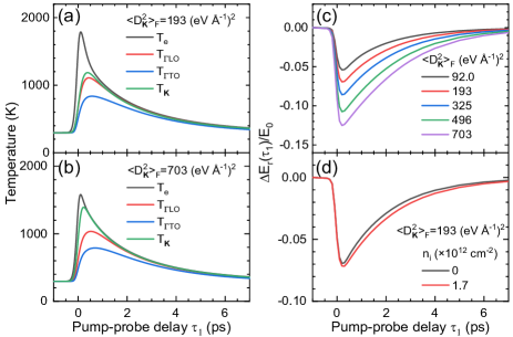
Figure 1: Simulation results of heavily doped graphene with $|\varepsilon_{F}|=0.43\,{\mathrm{eV}}$ for $F_{0}=100\,\mathrm{\mu J\,cm^{-2}}$. Temporal evolutions of $T_{\mathrm{e}}$ and $T_{\eta}$ for $\left\langle D_{\textbf{K}}^{2}\right\rangle_{\mathrm{F}}$=(a) 193 and (b) 703 $(\mathrm{eV\,\AA^{-1})^{2}}$. (c) $\left\langle D_{\textbf{K}}^{2}\right\rangle_{\mathrm{F}}$ dependence of $\Delta E_{\mathrm{r}}\left(\tau_{1}\right)/E_{0}$ of graphene calculated using temporal waveforms of THz probe pulse expressed by second derivative of Gaussian function, $\exp(-t^{2}/\tau_{\mathrm{pump}}^{2})$, with pulse durations of $2\tau_{\mathrm{pump}}=300\,\mathrm{fs}$. (d) $\Delta E_{\mathrm{r}}\left(\tau_{1}\right)/E_{0}$ at $\left\langle D_{\textbf{K}}^{2}\right\rangle_{\mathrm{F}}=193\,(\mathrm{eV\,\AA^{-1})^{2}}$ for $n_{\mathrm{i}}=0$ and $1.7\times 10^{12}\,\mathrm{cm}^{-2}$.

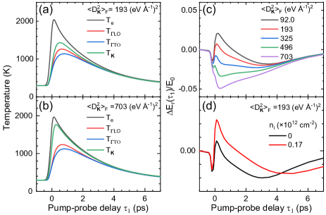
Figure 2: Simulation results of lightly doped graphene with $|\varepsilon_{F}|=0.15\,{\mathrm{eV}}$. Temporal evolutions of $T_{\mathrm{e}}$ and $T_{\eta}$ for $\left\langle D_{\textbf{K}}^{2}\right\rangle_{\mathrm{F}}$=(a) 92.0 and (b) 703 $(\mathrm{eV\,\AA^{-1})^{2}}$ for $F_{0}=100\,\mathrm{\mu J\,cm^{-2}}$. (c) $\left\langle D_{\textbf{K}}^{2}\right\rangle_{\mathrm{F}}$ dependence of $\Delta E_{\mathrm{r}}\left(\tau_{1}\right)/E_{0}$ of graphene. (d) $\Delta E_{\mathrm{r}}\left(\tau_{1}\right)/E_{0}$ at $\left\langle D_{\textbf{K}}^{2}\right\rangle_{\mathrm{F}}=193\,(\mathrm{eV\,\AA^{-1})^{2}}$ for $n_{\mathrm{i}}=0$ and $0.17\times 10^{12}\,\mathrm{cm}^{-2}$.

Figure 1(c) presents the $\left\langle D_{\textbf{K}}^{2}\right\rangle_{\mathrm{F}}$ dependence of the transient reflection change $\Delta E_{\mathrm{r}}(\tau_{1})/E_{0}$ calculated from the $\sigma(\omega,\tau_{1})$ using the THz probe pulse with $2\tau_{\mathrm{p}}=300\,\mathrm{fs}$. The sign of $\Delta E_{\mathrm{r}}(\tau_{1})/E_{0}$ remains negative indicating the negative photoconductivity as varying the $\left\langle D_{\textbf{K}}^{2}\right\rangle_{\mathrm{F}}$. The peak value of $\left|\Delta E_{\mathrm{r}}(\tau_{1})/E_{0}\right|$ increases monotonically as $\left\langle D_{\textbf{K}}^{2}\right\rangle_{\mathrm{F}}$ increases and effectively reflects the enhancement of $T_{\mathbf{K}}$.

Figure 2 depicts the simulation results on the lightly doped graphene with $|\varepsilon_{\mathrm{F}}|=0.15\,\mathrm{eV}$. Although the same phonon decay time $\tau_{\mathrm{ph}}=1\,\mathrm{ps}$ is used, the relaxation time of $T_{e}$ of the lightly doped graphene is longer than that of the heavily doped graphene owing to the weaker $R^{\mathrm{Net}}_{\eta}$ originated from the small density of state at the Fermi energy $\varepsilon_{\mathrm{F}}$. The sign of $\Delta E_{\mathrm{r}}(\tau_{1})/E_{0}$ indicated in Fig. 2(c) changes depending on $\left\langle D_{\textbf{K}}^{2}\right\rangle_{\mathrm{F}}$ in contrast with the heavily doped graphene. For a small $\left\langle D_{\textbf{K}}^{2}\right\rangle_{\mathrm{F}}=92.0\,(\mathrm{eV\AA^{-1})^{2}}$, $\Delta E_{\mathrm{r}}(\tau_{1})/E_{0}$ exhibits positive photoconductivity, which is transformed into negative photoconductivity as $\left\langle D_{\textbf{K}}^{2}\right\rangle_{\mathrm{F}}$ increases.

The different behaviors in $\Delta E_{\mathrm{r}}(\tau_{1})/E_{0}$ between the heavily and lightly doped graphene can be understood by considering the temperature dependence of the Drude weight $D\left(T_{\mathrm{e}}\right)$ of the graphene 2D MDF, which is the oscillator strength of free carrier absorption and plays a crucial role in carrier screening. As can be observed in Fig. 3(a), the chemical potential $\mu(T_{e})$ of graphene 2D MDF decreases with $T_{e}$, leading to the unique temperature dependence of $D\left(T_{\mathrm{e}}\right)$ according to $\varepsilon_{\mathrm{F}}$ Müller et al. (2009); Gusynin et al. (2009); Wagner et al. (2014); Frenzel et al. (2014); Yamashita and Otani (2021). In the case of a constant carrier relaxation rate, $D\left(T_{\mathrm{e}}\right)$ is expressed as

$$D\left(T_{e}\right)=\frac{2e^{2}}{\hbar^{2}}k_{\mathrm{B}}T_{e}\ln\left[2\cosh\left(\frac{\mu\left(T_{e}\right)}{2k_{\mathrm{B}}T_{e}}\right)\right].$$ (13)

The $D(T_{e})$ of the undoped graphene with $|\varepsilon_{\mathrm{F}}|=0.01\,\mathrm{eV}$ in Fig. 3(b) increases linearly with $T_{e}$, yielding positive photoconductivity. However, $D(T_{e})$ of the heavily doped graphene with $|\varepsilon_{\mathrm{F}}|=0.43\,\mathrm{eV}$ decreases slightly as $T_{e}$ increases and exhibits the minimum at around $T_{e}=2000\,\mathrm{K}$, contributing to the negative photoconductivity below $T_{e}=3000\,\mathrm{K}$. At temperatures below 3000 K, the maximum change in $D(T_{e})$ is only 13$\%$ and the temperature dependence of THz conductivity change is mainly dominated by of the carrier scattering with the SCOPs. In the lightly doped graphene, $D(T_{e})$ increases significantly above $T_{e}=1000\;\mathrm{K}$ and the contributions of $D(T_{e})$ and the carrier scattering with SCOPs to the photoconductivity compete with one another resulting in the positive and negative photoconductivity depending on $T_{e}$ and $\left\langle D_{\textbf{K}}^{2}\right\rangle_{\mathrm{F}}$.

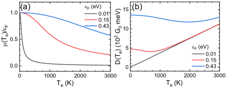
Figure 3: (a) $T_{e}$ dependence of chemical potential $\mu(T_{e})$ and Drude weight $D(T_{e})$ of graphene with $\varepsilon_{\mathrm{F}}=0.01,0.15,$ and $0.43\,\mathrm{eV}$.

We also investigated the effect of the charged impurity on the hot carrier dynamics in the heavily and lightly doped graphene because the charged impurity is one of the dominant scattering mechanism in graphene on substrate Tan et al. (2007); Chen et al. (2008b); Adam et al. (2007); Hwang et al. (2007). Figure 1(d) shows the $\Delta E_{\mathrm{r}}(\tau_{1})/E_{0}$ of the heavily doped graphene is almost unaffected by charged impurity scattering owing to the strong carrier screening effect. Here, the effective coupling constant $J_{a}$ of acoustic phonon is selected so that the DC conductivity is almost equal as shown in Table I. However, the $\Delta E_{\mathrm{r}}(\tau_{1})/E_{0}$ of the lightly doped graphene in Fig. 2(d) changes significantly by the presence of the low charged impurity concentration $n_{\mathrm{i}}=0.17\times 10^{12}\,\mathrm{cm^{-2}}$, indicating a crossover from the negative $\Delta E_{\mathrm{r}}(\tau_{1})/E_{0}$ to the positive one and the reduction of the carrier scattering due to the enhanced carrier screening effect. Therefore, the information of the accurate charged impurity concentration is required to derive the $\left\langle D_{\textbf{K}}^{2}\right\rangle_{\mathrm{F}}$ from $\Delta E_{\mathrm{r}}(\tau_{1})/E_{0}$ of lightly doped graphene. These findings indicate that heavily doped graphene is suitable for the determination of $\left\langle D_{\textbf{K}}^{2}\right\rangle_{\mathrm{F}}$ from $\Delta E_{\mathrm{r}}(\tau_{1})/E_{0}$.

III Experimental results

The graphene sample (Graphene Platform Corporation) that was examined in this study was prepared using chemical vapor deposition. The single-layer graphene (area: 10 mm$\times$10 mm) was transferred to a PET substrate. Raman scattering measurements confirmed the single-layer thickness of the sample and their low defect density.

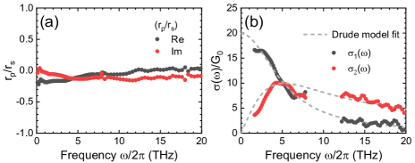
Figure 4: (a) $(r_{\mathrm{p}}/r_{\mathrm{s}})$ of graphene at equilibrium measured by THz-TDSE. (b) $\sigma(\omega)$ at equilibrium. The dotted line is the fitting curve of the simple Drude model.

The equilibrium THz conductivity of the sample at room temperature ($T_{0}=295\,{\mathrm{K}}$) was characterized by ultrabroadband THz time domain spectroscopic ellipsometry (THz-TDSE) (see Section I in the SM for details), which enabled the broad Drude peak to be captured directly by measuring the ratio of the reflection coefficient $r_{\mathrm{p}}(\omega)/r_{\mathrm{s}}(\omega)$ in the frequency range between 1.0 and 20 THz Yamashita et al. (2014), as illustrated in Fig. 4. The fitting of the THz conductivity spectrum obtained from $r_{\mathrm{p}}(\omega)/r_{\mathrm{s}}(\omega)$ by the Drude model allows us to determine the Drude weight $D_{0}$ and carrier relaxation rate $\Gamma_{0}$ for the equilibrium state at room temperature $T_{0}=295\,\mathrm{K}$ accurately. We estimated $D_{0}=1.36\times 10^{3}G_{0}$ and $\Gamma_{0}=21.4\,\mathrm{meV}$, respectively. Here, $G_{0}=2e^{2}/h$ is the quantum conductance. The corresponding Fermi energy is $|\varepsilon_{\mathrm{F}}|=0.43\,\mathrm{eV}$, indicating that the sample is heavily doped and suitable for estimating the EPC strength. The carrier concentration $n_{\mathrm{c}}$ at $T_{e}=0\,\mathrm{K}$ and the DC conductivity at $T_{0}$ were estimated as $n_{\mathrm{c}}=1.1\times 10^{13}\mathrm{cm^{-2}}$ and $\sigma_{\mathrm{DC}}=20G_{0}$, respectively, where we used $v_{\mathrm{F}}=1.1\times 10^{6}\,\mathrm{m\,s^{-1}}$ considering the carrier and dielectric screening effect in heavily doped graphene on PET substrateElias et al. (2011).

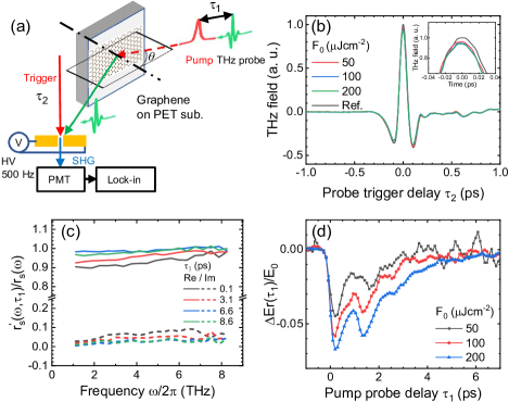
Figure 5: (a) Schematic of reflection-type OPTP setup. Pump: pump pulse, Trigger: trigger pulse, SHG: second harmonic generation, HV: high voltage, PMT: photomultiplier tube. (b) Temporal waveforms of THz probe pulse measured at $\tau_{1}=$ 0.1 ps. (c) Frequency dependence of $(r_{\mathrm{s}}^{\prime}(\omega,\tau_{1})/r_{\mathrm{s}}(\omega))$ at $\tau_{1}$ = 0.1, 3.1, 6.6, and 8.6 ps at $F_{0}=200\,\mu J\,cm^{-2}$. (d) Pump fluence dependence of $\Delta E(\tau_{1})/E_{0}$.

Figure 5(a) presents the optical setup of the reflection-type OPTP used in the experiment. Amplified femtosecond laser pulses (1kHz repetition rate, 785 nm center wavelength) are used to generate ultrabroadband THz probe pulses from laser-excited air plasmaXie et al. (2006). S-polarized pump pulses with a pulse duration of 220 fs are loosely focused and excited the graphene sample at an incident angle of $\theta=60^{\circ}$ and the created hot carrier state was probed by s-polarized THz pulses with a pump probe time delay $\tau_{1}$. The temporal waveforms of the reflected THz probe pulses are measured by air breakdown coherent detection, which detects the second harmonic generation of the trigger pulse induced by the THz electric fieldDai et al. (2006). Figure 5(b) depicts the temporal waveforms of the THz probe pulse reflected from the photoexcited graphene. When the pump fluence is increased, the peak amplitude of THz probe decreases slightly, indicating negative photoconductivity. The ratio of the reflection coefficient $r_{\mathrm{s}}^{\prime}(\omega,\tau_{1})/r_{\mathrm{s}}(\omega)$ of graphene with and without pump fluence $F_{0}=200\,\mathrm{\mu J\,cm^{-2}}$ calculated by Fourier transformation of the THz waveforms at different $\tau_{1}$ values, as plotted in Fig. 5(c), decreases and then recovers to the equilibrium reflecting the rise and subsequent relaxation process of the hot carrier dynamics, and this was used for the calculation of $\sigma(\omega,\tau_{1})$ (see Section II in the SM for details). Figure 5(d) presents the fluence dependence of $\Delta E_{\mathrm{r}}(\tau_{1})/E_{0}$, which exhibits multiple negative peaks around $\tau_{1}=0.2,1.4,2.3\,\mathrm{ps}$ owing to the multiple reflections inside the PET substrate. As $F_{0}$ increases, the peak height $\Delta E_{\mathrm{r}}(\tau_{1})/E_{0}$ increases but it exhibits saturation behavior with an increased relaxation time.

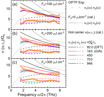
Figure 6: Pump fluence dependence of $\sigma(\omega,\tau_{1})$ (orange symbols) of heavily doped graphene obtained from for $F_{0}=$(a)100, (b)200 and (c)300$\,\mathrm{\mu J\,cm^{-2}}$. The gray solid and dashed lines correspond to the calculated $\sigma(\omega)$ at equilibrium. The black, red, purple, green and blue lines correspond to $\sigma(\omega,\tau_{1})$ at $\tau_{1}=0.1$ ps using $\left\langle D_{\textbf{K}}^{2}\right\rangle_{\mathrm{F}}=92.0,193,450,703$ and 946 $(\mathrm{eV\,\AA^{-1})^{2}}$, respectively.

Figures 6(a)-(c) present the pump fluence dependence of $\sigma(\omega,\tau_{1})$ measured at $\tau_{1}=0.1\,\mathrm{ps}$. We observe the reduction of the THz conductivity indicating the large negative photoconductivity with non-Drude behavior as $F_{0}$ increases and $\sigma(\omega,\tau_{1})$ for $F_{0}=200\,\mathrm{\mu J\,cm^{-2}}$ reaches less than half of that at the equilibrium (gray curve), indicating a significant increase in the carrier scattering by SCOPs at high temperatures. It is found that $\sigma(\omega,\tau_{1})$ for $\left\langle D_{\mathbf{\Gamma}}^{2}\right\rangle_{\mathrm{F}}$ by the DFT (black curve) and GW (blue curve) calculations can not reproduce the observed negative photoconductivity, even if the SA effect is not considered. On the other hand, $\sigma(\omega,\tau_{1})$ for $\left\langle D_{\mathbf{\Gamma}}^{2}\right\rangle_{\mathrm{F}}=703$ and $946\,(\mathrm{eV\,\AA^{-1})^{2}}$ show the larger deviation than that for $\left\langle D_{\mathbf{\Gamma}}^{2}\right\rangle_{\mathrm{F}}=450\,(\mathrm{eV\,\AA^{-1})^{2}}$.

Figures 7(a)-(c) depict the comparison of $\Delta E_{\mathrm{r}}(\tau_{1})/E_{0}$ between the experiment and calculations, which is significantly dependent on $\left\langle D_{\mathbf{K}}^{2}\right\rangle_{\mathrm{F}}$ and the pump fluence $F_{0}$. For $\left\langle D_{\mathbf{K}}^{2}\right\rangle_{\mathrm{F}}$ by the DFT and GW calculations, the peak height and temporal evolution of $\Delta E_{\mathrm{r}}(\tau_{1})/E_{0}$ differ significantly from the experimental values and the higher values $\left\langle D_{\mathbf{K}}^{2}\right\rangle_{\mathrm{F}}=450$–$946\,(\mathrm{eV\,\AA^{-1}})^{2}$ are required to reproduce the $\Delta E_{\mathrm{r}}(\tau_{1})/E_{0}$. By comparing $\sigma(\omega,\tau_{1})$ and $\Delta E_{\mathrm{r}}(\tau_{1})/E_{0}$ with the calculation in Figs. 6 and 7, we estimated $\left\langle D_{\mathbf{K}}^{2}\right\rangle_{\mathrm{F}}\approx 450\,(\mathrm{eV\,\AA^{-1}})^{2}$ and $\tau_{\mathrm{ie}}=116\,\mathrm{fs}$, at which the calculation (blue curves) best fits the experimental results.

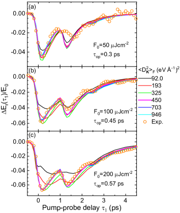
Figure 7: Comparison of $\Delta E_{\mathrm{r}}(\tau_{1})/E_{0}$ between experiment and calculations for different EPCs for pump fluence $F_{0}=$(a)50, (b)100 and (c)200$\,\mathrm{\mu Jcm^{-2}}$. The red open circles represent the experimental $\Delta E_{\mathrm{r}}(\tau_{1})/E_{0}$. The solid curves correspond to the $\Delta E_{\mathrm{r}}(\tau_{1})/E_{0}$ calculated using $\left\langle D_{\mathbf{\Gamma}}^{2}\right\rangle_{\mathrm{F}}=92.0\mathrm{\,(DFT,black)}$, $193\,(\mathrm{GW,red})$, $\mathrm{325\,(green)}$, $\mathrm{450\,(purple)}$, $\mathrm{703\,(blue)}$ and $\mathrm{946\,(light\,blue)}\,(\mathrm{eV\,\AA^{-1})^{2}}$, respectively.

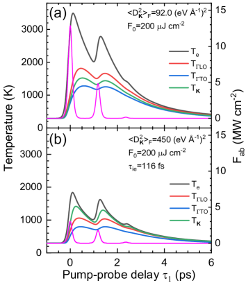
Figure 8: Temporal evolution of $T_{e}$ and $T_{\eta}$ calculated for $\left\langle D_{\mathbf{K}}^{2}\right\rangle_{\mathrm{F}}=$ (a) 92.0and (b) $450\,(\mathrm{eV\,\AA^{-1})^{2}}$. The red curve is the absorbed pump intensity $F_{\mathrm{ab}}$, calculated considering the SA effect.

In this case, the obtained $\tau_{\mathrm{ie}}=116\,\mathrm{fs}$ corresponds to the saturated pump intensity $I_{s}=1.0$ and $1.7\times 10^{8}\,\mathrm{W\,cm^{-2}}$ for $\alpha_{\mathrm{inter}}$ and $A^{\mathrm{s*}}_{12}$ respectively, which is slightly smaller than the reported value in Ref. Hyung et al. (2012); Marini et al. (2017).

Figure 8 presents the temporal evolution of $T_{e}$ and $T_{\eta}$ calculated for $\left\langle D_{\mathbf{K}}^{2}\right\rangle_{\mathrm{F}}=92.0$ and $450\,(\mathrm{eV\,\AA^{-1})^{2}}$ under the pump fluence $F_{0}=200\,\mathrm{\mu J\,cm^{-2}}$ indicating that hot carrier and phonon dynamics are significantly dependent on the EPC. For $\left\langle D_{\mathbf{K}}^{2}\right\rangle_{\mathrm{F}}=92.0\,(\mathrm{eV\,\AA^{-1})^{2}}$ as shown in Fig. 8(a), the hot carrier temperature increases beyond $T_{e}$=3000 K, and $T_{\mathbf{K}}$ followed $T_{e}$ slowly owing to the weak EPC and reaches up to $T_{\mathbf{K}}\approx 1500\,\mathrm{K}$. In this high temperature range, the carrier scattering by optical phonons is dominant and the Drude weight $D(T_{e})$ makes the positive contribution to $\sigma(\omega,\tau_{1})$ in contrast to the carrier scattering. The competition of these factors leads to broader peaks of $\Delta E_{\mathrm{r}}(\tau_{1})/E_{0}$ for DFT (black line) in Fig. 7(c) than those of $T_{\mathrm{\eta}}$ in Fig. 8(a). For $\left\langle D_{\mathbf{K}}^{2}\right\rangle_{\mathrm{F}}=450\,(\mathrm{eV}\mbox{\AA}^{-1})^{2}$ as seen in Fig. 8(b), the hot carrier temperature increases up to only $T_{e}\approx$2000 K and $T_{\mathbf{K}}$ follows $T_{e}$ rapidly and reaches up to $T_{\mathbf{K}}\approx 1400\,K$ owing to the SA effect and strong EPC. In this case, $D(T_{e})$ makes the same contribution to $\sigma(\omega,\tau_{1})$ as the optical phonon scattering, resulting in sharper peaks of $\Delta E_{\mathrm{r}}(\tau_{1})/E_{0}$ and a successful reproduction of the experimental results. Furthermore, the frequency dependence of $\sigma(\omega,\tau_{1})$ at $\tau_{1}$ = 0.1 ps in Fig. 6 deviates from the simple Drude model as $F_{0}$ increases. This originates from the rapid temporal variation in the carrier temperature and scattering rate during the THz probing time following the photoexcitation, and the calculation with $\left\langle D_{\mathbf{K}}^{2}\right\rangle_{\mathrm{F}}=450\,(\mathrm{eV\AA^{-1}})^{2}$ effectively reproduces the observed large negative photoconductivity with non-Drude behavior. This indicates that most photoexcited carriers are recombined and the quasi-equilibrium hot carrier state is almost established at $\tau_{1}=0.1\,\mathrm{ps}$ owing to the strong Auger recombination in the heavily doped graphene, as reported in Ref. Gierz et al. (2013). The parameters used in the calculation are displayed in Table II.

Table 2: Parameters used in calculation of $\sigma(\omega,\tau_{1})$ and $\Delta E_{\mathrm{r}}(\tau_{1})/E_{0}$ in Figs. 6, 7 and 8^a.

$\left\langle D_{\mathrm{K}}^{2}\right\rangle_{\mathrm{F}}$ $(\mathrm{eV}\mbox{\AA}^{-1})^{2}$	$\tau_{\mathrm{ie}}$ (fs)	$I_{\mathrm{s}}(\mathrm{W\,cm^{-2}})$	$n_{\mathrm{i}}\,(\mathrm{cm^{-2}})$	$\lambda_{\mathbf{K}}(\varepsilon_{\mathrm{F}})$
92.0	–	–	$1.15\times 10^{12}$	0.02
193	–	–	$1.13\times 10^{12}$	0.04
450	116	$1.72\times 10^{8}$	$1.09\times 10^{12}$	0.09
703	210	$0.53\times 10^{8}$	$1.05\times 10^{12}$	0.14
946	299	$0.26\times 10^{8}$	$1.01\times 10^{12}$	0.19

^a The values of $\left\langle D_{\bf{\Gamma}}^{2}\right\rangle_{\mathrm{F}}$, $J_{\mathrm{a}}$ and $\rho_{\mathrm{s}}$ are set to $\left\langle D_{\mathbf{\Gamma}}^{2}\right\rangle_{\mathrm{F}}=45.6\,(\mathrm{eV}\mbox{\AA}^{-1})^{2}$, $J_{\mathrm{a}}=30.0\,(\mathrm{eV})$ and $\rho_{\mathrm{s}}=40.0\,(\Omega)$, respectively. The charged impurity concentration $n_{\mathrm{i}}$ is selected to provide the same DC conductivity $\sigma_{\mathrm{DC}}=20.0G_{0}$ at equilibrium for $T_{0}=295\,\mathrm{K}$.

IV Discussion

Based on the fitting of $\Delta E_{\mathrm{r}}(\tau_{1})/E_{0}$ by the calculation considering the EPC, we estimated the phenomenological phonon decay time due to lattice anharmonicity as $\tau_{\mathrm{ph}}=0.3,0.45$ and $0.57\,\mathrm{ps}$ for $F_{0}=50,100$ and $200\,\mathrm{\mu J\,cm^{-2}}$, respectively. Refs. Kang et al. (2010); Gao et al. (2011) reported longer $\tau_{\mathrm{ph}}=0.8$–1.5$\,\mathrm{ps}$ for graphene on a $\mathrm{SiO_{2}}$ substrate. However, these values were determined from the simple fitting of transient absorption or anti-stokes Raman intensity by exponential function and do not consider the EPC. The simple fitting of $\Delta E_{\mathrm{r}}(\tau_{1})/E_{0}$ with exponential curve results in $\tau_{\mathrm{ph}}=$ 1.15–1.5 ps which are comparable to the reported values. The theoretical study reported the phonon decay time $\tau_{\mathrm{ph}}\approx$ 3.5 and 4.5 ps for $\mathbf{\Gamma}$ and $\mathbf{K}$ phonon by only considering the anharmonicity of lattice in graphene without substrate Bonini et al. (2007). Therefore, the obtained $\tau_{\mathrm{ph}}$ indicates the dominant contribution of substrate for the optical phonon decay channel.

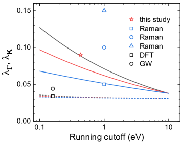
Figure 9: Flow of dimensionless coupling constants $\lambda_{\mathbf{\Gamma}}$ and $\lambda_{\mathbf{K}}$ (three dashed and solid curves, respectively) for three values of $\epsilon_{\mathrm{av}}$=1, 2, and 5. The red and blue symbols correspond to the $\lambda_{\mathbf{K}}$ determined in this study ($\epsilon_{\mathrm{av}}=2$) and by Raman studies ($\epsilon_{\mathrm{av}}=5$) from Ref. Basko et al. (2009) (blue open square and circle) and Ref. Froehlicher and Berciaud (2015) (blue open triangle). The black open circle and square correspond to $\lambda_{\mathbf{K}}$ by the DFT Piscanec et al. (2004); Basko et al. (2009) and GW Lazzeri et al. (2008); Grüneis et al. (2008); Basko et al. (2009) calculations ($\epsilon_{\mathrm{av}}=1$), respectively.

The dimensionless coupling constants $\lambda_{\mathbf{\Gamma}}$ and $\lambda_{\mathbf{K}}$ for the optical phonons near the $\mathbf{\Gamma}$ and $\mathbf{K}$ points, respectively, are useful for comparing the EPC strengths determined from various experiments and calculations, which are defined as Basko et al. (2009)

$$\lambda_{\mathbf{\Gamma},\mathbf{K}}=\frac{F^{2}_{\mathbf{\Gamma},\mathbf{K}}A_{\mathrm{u.c.}}}{2M\hbar\omega_{\mathbf{\Gamma},\mathbf{K}}v_{F}^{2}}.$$ (14)

In the above, $M\approx 2.00\times 10^{-26}\,\mathrm{kg}$ is the mass of the carbon atom and $A_{\mathrm{u.c.}}\approx 5.24\,\mbox{\AA}^{2}$ is the unit-cell area. $F^{2}_{\mathbf{\Gamma}}$ and $F^{2}_{\mathbf{K}}$ have the dimensionality of a force and are the proportionality coefficients between the change in the effective Hamiltonian and lattice displacement along the corresponding phonon mode. Subsequently, the matching rules are expresses as $F^{2}_{\mathbf{\Gamma}}=4\left\langle D_{\mathbf{\Gamma}}^{2}\right\rangle_{\mathrm{F}}$ and $F^{2}_{\mathbf{K}}=2\left\langle D_{\mathbf{K}}^{2}\right\rangle_{\mathrm{F}}$. Note that $\lambda_{\mathbf{K}}$ is subject to Coulomb renormalization, which implies that $\lambda_{\mathbf{K}}$ is dependent on the electronic energy scale, such as the electron energy, Fermi energy, or temperature T, whichever is larger: $\lambda_{\mathbf{K}}=\lambda_{\mathbf{K}}(\mathrm{max}\{|\varepsilon|,|\varepsilon_{\mathrm{F}}|,|T|\})$. From $\left\langle D_{\mathbf{K}}^{2}\right\rangle_{\mathrm{F}}\approx 450\,\mathrm{(eV\,A^{-1})^{2}}$, we estimated $\lambda_{\mathbf{K}}(\varepsilon_{\mathrm{F}})\approx 0.09$ using Eqs. (13) and (14). Figure 9 presents the flow of $\lambda_{\mathbf{\Gamma}}$ and $\lambda_{\mathbf{K}}$ for different background static dielectric constants $\epsilon_{\mathrm{av}}=(1+\epsilon_{\mathrm{s}})/2=1$, 2, and 5 calculated by solving the renormalization group equation in Ref. Basko and Aleiner (2008), which sum up the leading logarithmic corrections and go beyond the Hartree–Fock approximation. The bare values of the dimensionless EPCs $\lambda_{\mathbf{\Gamma}}=0.031$ and $\lambda_{\mathbf{K}}=0.038$ were selected to satisfy the relation $\lambda_{\mathbf{\Gamma}}/\lambda_{\mathbf{K}}=\omega_{\mathbf{K}}/\omega_{\mathbf{\Gamma}}$ and to reproduce the experimental value $\lambda_{\mathbf{\Gamma}}=0.031$ Froehlicher and Berciaud (2015). The renormalization group analysis demonstrated that, although $\lambda_{\mathbf{\Gamma}}$ was almost constant, $\lambda_{\mathbf{K}}$ was strongly dependent on the energy scale as well as $\epsilon_{\mathrm{av}}$. The obtained $\lambda_{\mathbf{K}}(\varepsilon_{\mathrm{F}})=0.09$ slightly larger than the calculated value of $\lambda_{\mathbf{K}}(\varepsilon_{\mathrm{F}})=0.073$. According to the ratio of the $\lambda({\omega_{\mathbf{K}}})/\lambda_{\mathbf{K}}(\varepsilon_{\mathrm{F}})=1.21$ for $\epsilon_{\mathrm{av}}=2$ in Fig. 9, we obtained $\lambda({\omega_{\mathbf{K}}})=0.11$, which is a factor of 3.2 larger than the DFT value $\lambda_{\mathbf{K}}({\omega_{\mathbf{K}}})=0.034$. Raman studies Ferrari et al. (2006b); Das et al. (2008, 2009); Berciaud et al. (2009b); Froehlicher and Berciaud (2015) using a field effect transistor based on the polymer electrolyte ($\epsilon_{\mathrm{av}}=5$) reported $\lambda_{\mathbf{\Gamma}}=$0.028 and 0.031 from the ratio of the area between G and the 2D peak, which were comparable to $\lambda_{\mathbf{\Gamma}}=0.028$ by the DFT calculation of $\left\langle g_{\mathbf{\Gamma}}^{2}\right\rangle_{\mathrm{F}}$ using Eq. (14). However, $\lambda_{\mathbf{K}}(E_{\mathrm{L}}/2)$ ranged between 0.05 and 0.15 as seen in Fig. 9, where $E_{L}$ is the laser excitation energy (for a typical Raman measurement $E_{\mathrm{L}}/2\sim 1\mathrm{eV}$). The corresponding $\lambda_{\mathbf{K}}(\omega_{\mathbf{K}})$ are estimated as 0.063 and 0.19. The lower limit value is comparable to the calculated $\lambda_{\mathbf{K}}(\omega_{\mathbf{K}})$ for $\epsilon_{\mathrm{av}}=5$. Although Raman spectroscopy is a powerful tool for the determination of $\lambda_{\mathbf{K}}(\omega_{\mathbf{K}})$ as well as $\lambda_{\mathbf{\Gamma}}(\omega_{\mathbf{K}})$, it requires the accurate estimation of the gate capacitance of FET device which are not required in OPTP experiments.

V Conclusion

In conclusion, we investigated the EPC of the optical phonons near the $\mathbf{K}$ point of heavily doped graphene on PET substrate and the hot carrier dynamics using a combination of the time-resolved THz spectroscopy and numerical simulations. The hot carrier dynamics in heavily doped graphene on PET substrate is less sensitive to the extrinsic charged impurity and surface polar phonons of the substrate and is dominated by the electron-optical phonon interactions. According to the quantitative analysis based on the BTE and comprehensive temperature model considering the SA effect on pump fluence, the $\Delta E(\tau_{1})/E_{0}$ value can be used for the determination of the EPC in graphene. The estimated $\left\langle D_{\mathbf{K}}^{2}\right\rangle_{\mathrm{F}}\approx 450\,\mathrm{(eV\AA^{-1})^{2}}$ indicates the strong renormalization by e-e interaction and the corresponding dimensionless coupling constant $\lambda_{\mathbf{K}}(E_{\mathrm{F}})\approx 0.09$ slightly larger than the calculation by the renormalization group theory. The extension of the simulation model for the undoped or lightly doped graphene on various substrate requires the accurate estimation of charged impurities and surface polar phonons of the substrate is a future issue that will be important to the development of graphene optoelectronic devices.