Integrability of the conformal loop ensemble

Abstract

We demonstrate that the conformal loop ensemble (CLE) has a rich integrable structure by establishing exact formulas for two CLE observables. The first describes the joint moments of the conformal radii of loops surrounding three points for CLE on the sphere. Up to normalization, our formula agrees with the imaginary DOZZ formula due to Zamolodchikov (2005) and Kostov-Petkova (2007), which is the three-point structure constant of certain conformal field theories that generalize the minimal models. This verifies the CLE interpretation of the imaginary DOZZ formula by Ikhlef, Jacobsen and Saleur (2015). Our second result is for the moments of the electrical thickness of CLE loops first considered by Kenyon and Wilson (2004). Our proofs rely on the conformal welding of random surfaces and two sources of integrability concerning CLE and Liouville quantum gravity (LQG). First, LQG surfaces decorated with CLE inherit a rich integrable structure from random planar maps decorated with the $O(n)$ loop model. Second, as the field theory describing LQG, Liouville conformal field theory is integrable. In particular, the DOZZ formula and the FZZ formula for its structure constants are crucial inputs to our results.

1 Introduction

The conformal loop ensemble ($\operatorname{CLE}$) is a canonical conformally invariant probability measure on infinite collections of non-crossing loops, where each loop looks like a Schramm-Loewner evolution (SLE). CLE has been proved or conjectured to be the scaling limit of many important loop models in two dimensional statistical physics, such as percolation, Ising model, the $O(n)$-loop model, and the random cluster model. There has been an extensive literature on CLE since the foundational work of Sheffield [She09] and Sheffield-Werner [SW12]; see e.g. [ALS20, BH19, CN08, GMQ18, KS16, KW16, Lup19, MSW14, MWW16, MWW15, MSW17, SSW09, WW13].

In this paper we demonstrate that CLE has a rich integrable structure by establishing exact formulas for two CLE observables. The first describes the joint moments of the conformal radii of loops surrounding three points for CLE on the sphere. Our formula agrees with the imaginary DOZZ formula [Zam05, KP07] up to normalization, which verifies the geometric interpretation of this formula proposed in [IJS16]. Our second formula is for the moments of the electrical thickness of CLE loops first considered by Kenyon and Wilson [KW04]. We will focus on the simple-loop regime $\kappa\in(8/3,4]$ and treat the non-simple loop regime $\kappa\in(4,8)$ in a subsequent paper. See Sections 1.1 and 1.3 for the precise statements of our results.

Our proofs rely on two sources of integrability concerning CLE and Liouville quantum gravity (LQG). First, LQG surfaces decorated with CLE inherit a rich integrable structure from random planar maps decorated with the $O(n)$ loop model, as exhibited in [BBCK18, CCM20, MSW20]. Second, as the field theory describing LQG, Liouville conformal field theory (LCFT) is integrable. In particular, the DOZZ formula [KRV17] and FZZ formula [ARS21] for its structure constants are crucial inputs to our results. See Section 1.2 for a summary of our method.

This paper is part of our program exploring the connections between the integrabilities of SLE, LQG and LCFT. In Section 1.4 we discuss future works and list some open questions.

1.1 Three-point correlation function for CLE and the imaginary DOZZ formula

For $\kappa\in(8/3,4]$, $\operatorname{CLE}_{\kappa}$ on a simply connected domain $D\subsetneq\mathbbm{C}$ can be characterized by the domain Markov property and conformal invariance [SW12]. In this case the loops are disjoint Jordan curves. The full-plane $\operatorname{CLE}_{\kappa}$ can be obtained by sending $D\to\mathbbm{C}$. Viewed as a loop ensemble living on the extended complex plane $\hat{\mathbbm{C}}=\mathbbm{C}\cup\{\infty\}$, the full-plane $\operatorname{CLE}_{\kappa}$ is invariant under conformal transformations on $\hat{\mathbbm{C}}$ [KW16]. Hence we also call a full-plane $\operatorname{CLE}_{\kappa}$ a $\operatorname{CLE}_{\kappa}$ on the sphere.

Suppose $\Gamma$ is a full-plane $\operatorname{CLE}_{\kappa}$. Fix three distinct points $z_{1},z_{2},z_{3}\in\mathbbm{C}$. There are infinitely many loops that separate $z_{1}$ and $\{z_{2},z_{3}\}$. For each such loop $\eta$, we let $D_{\eta}$ be the simply connected component of $\hat{\mathbbm{C}}\setminus\eta$ containing $z_{1}$. (The domain $D_{\eta}$ could contain $\infty$.) There exists a loop $\eta_{1}$ with the largest $D_{\eta}$, which we call the outermost loop separating $z_{1}$ and $z_{2},z_{3}$. For $i=2,3$, we similarly let $\eta_{i}$ be the outermost loop in $\Gamma$ separating $z_{i}$ and $\{z_{1},z_{2},z_{3}\}\setminus\{z_{i}\}$.

Given a simple loop $\eta$ on $\hat{\mathbbm{C}}$ surrounding a point $z\in\mathbbm{C}$ the conformal radius $\mathrm{CR}(\eta,z)$ of $\eta$ viewed from $z$ is defined as follows. Let $\mathbbm{D}$ be the unit disk. Let $D_{\eta}$ be the connected component of $\hat{\mathbbm{C}}\setminus\eta$ containing $z$ and let $\psi:\mathbbm{D}\rightarrow D_{\eta}$ be a conformal map such that $\psi(0)=z$. Then $\mathrm{CR}(\eta,z)$ is defined by $|\psi^{\prime}(0)|$. Given $\eta_{i}$ and $z_{i}$ defined above, we call the joint moment generating function $\mathbbm{E}[\prod_{i=1}^{3}\mathrm{CR}(\eta_{i},z_{i})^{\lambda_{i}}]$ the three-point correlation function for $\operatorname{CLE}_{\kappa}$ on the sphere.

Lemma 1.1.

There exists a function ${C^{\operatorname{CLE}}_{\kappa}(\lambda_{1},\lambda_{2},\lambda_{3})}\in(0,\infty]$ such that

$$\mathbbm{E}[\prod_{i=1}^{3}\mathrm{CR}(\eta_{i},z_{i})^{\lambda_{i}}]={C^{\operatorname{CLE}}_{\kappa}(\lambda_{1},\lambda_{2},\lambda_{3})}\prod_{i=1}^{3}|z_{i}-z_{i+1}|^{\lambda_{i}+\lambda_{i+1}-\lambda_{i+2}},$$ (1.1)

where we identify $z_{j}$ with $z_{j-3}$ and $\lambda_{j}$ with $\lambda_{j-3}$.

Proof.

This follows from the conformal invariance of full-plane $\operatorname{CLE}_{\kappa}$, the scaling property of conformal radius, and the fact that any triple of points on the plane are conformally equivalent. ∎

We call ${C^{\operatorname{CLE}}_{\kappa}(\lambda_{1},\lambda_{2},\lambda_{3})}$ the structure constant for $\operatorname{CLE}_{\kappa}$ on the sphere. This terminology and the three-point correlation function above are inspired by Liouville conformal field theory (LCFT), which is the quantum field theory with Liouville action introduced by Polyakov [Pol81]. It was recently made rigorous in [DKRV16] and follow-up works [HRV18, DRV16, GRV19, Rem18]; see Section 2.2 for more background. For LCFT, the three-point correlation function on the sphere, which depends on three points $z_{1},z_{2},z_{3}$ on $\mathbbm{C}$ and three parameters $\alpha_{1},\alpha_{2},\alpha_{3}\in\mathbbm{R}$, is also of the form (1.1) where the dependence on $(\alpha_{1},\alpha_{2},\alpha_{3})$ is encoded in its structure constant. It was first proposed in theoretical physics [DO94, ZZ96] and then rigorously proved in [KRV17] that the structure constant has the following remarkable expression known as the DOZZ formula. Suppose $\gamma\in(0,2)$ is the coupling parameter for LCFT and $Q=\frac{\gamma}{2}+\frac{2}{\gamma}$ is its background charge. The DOZZ formula (with cosmological constant being 1) is given by

$$C^{\mathrm{DOZZ}}_{\gamma}(\alpha_{1},\alpha_{2},\alpha_{3})=\mathopen{}\mathclose{{}\left(\frac{\pi(\frac{\gamma}{2})^{2-\gamma^{2}/2}\Gamma(\frac{\gamma^{2}}{4})}{\Gamma(1-\frac{\gamma^{2}}{4})}}\right)^{\frac{2Q-\overline{\alpha}}{\gamma}}\frac{\Upsilon_{\frac{\gamma}{2}}^{\prime}(0)\Upsilon_{\frac{\gamma}{2}}(\alpha_{1})\Upsilon_{\frac{\gamma}{2}}(\alpha_{2})\Upsilon_{\frac{\gamma}{2}}(\alpha_{3})}{\Upsilon_{\frac{\gamma}{2}}(\frac{\overline{\alpha}}{2}-Q)\Upsilon_{\frac{\gamma}{2}}(\frac{\overline{\alpha}}{2}-\alpha_{1})\Upsilon_{\frac{\gamma}{2}}(\frac{\overline{\alpha}}{2}-\alpha_{2})\Upsilon_{\frac{\gamma}{2}}(\frac{\overline{\alpha}}{2}-\alpha_{3})},$$ (1.2)

where $\overline{\alpha}=\sum\alpha_{j}$ and $\Upsilon_{\frac{\gamma}{2}}(z)$ is an explicit entire function. The function $\Upsilon_{\frac{\gamma}{2}}(z)$ is specified by

$$\log\Upsilon_{\frac{\gamma}{2}}(z)=\int_{0}^{\infty}\mathopen{}\mathclose{{}\left(\mathopen{}\mathclose{{}\left(\frac{Q}{2}-z}\right)^{2}e^{-t}-\frac{(\sinh((\frac{Q}{2}-z)\frac{t}{2}))^{2}}{\sinh(\frac{t\gamma}{4})\sinh(\frac{t}{\gamma})}}\right)\frac{dt}{t}\quad\text{ for }0<\operatorname{Re}(z)<Q.$$

Moreover $\Upsilon_{\frac{\gamma}{2}}$ satisfies the following shift relations:

$$\Upsilon_{\frac{\gamma}{2}}(z+\frac{\gamma}{2})=\frac{\Gamma(\frac{\gamma}{2}z)}{\Gamma(1-\frac{\gamma}{2}z)}(\frac{\gamma}{2})^{1-\gamma z}\Upsilon_{\frac{\gamma}{2}}(z)\quad\text{and}\quad\Upsilon_{\frac{\gamma}{2}}(z+\frac{2}{\gamma})=\frac{\Gamma(\frac{2}{\gamma}z)}{\Gamma(1-\frac{2}{\gamma}z)}(\frac{\gamma}{2})^{\frac{4}{\gamma}z-1}\Upsilon_{\frac{\gamma}{2}}(z).$$

Our first main result is an explicit formula for ${C^{\operatorname{CLE}}_{\kappa}(\lambda_{1},\lambda_{2},\lambda_{3})}$ which is closely related to the DOZZ formula. Indeed, under a certain parameter identification their product is factorized.

Theorem 1.2.

For $\kappa\in(\frac{8}{3},4]$, the structure constant ${C^{\operatorname{CLE}}_{\kappa}(\lambda_{1},\lambda_{2},\lambda_{3})}<\infty$ if and only if $\lambda_{1},\lambda_{2},\lambda_{3}>\frac{3\kappa}{32}-1+\frac{2}{\kappa}$. In this case, set $\gamma=\sqrt{\kappa}$ and $Q=\frac{\gamma}{2}+\frac{2}{\gamma}$. Let $\alpha_{i}$ be a root of $\alpha(Q-\frac{\alpha}{2})-2=\lambda_{i}$ for $i=1,2,3$. Then

$${C^{\operatorname{CLE}}_{\kappa}(\lambda_{1},\lambda_{2},\lambda_{3})}=\frac{\prod_{i=1}^{3}N_{\gamma}(\alpha_{i})}{C^{\mathrm{DOZZ}}_{\gamma}(\alpha_{1},\alpha_{2},\alpha_{3})},$$ (1.3)

where

$$N_{\gamma}(\alpha)=\mathopen{}\mathclose{{}\left(-\pi\cos(\frac{4\pi}{\gamma^{2}})\frac{\Gamma(\frac{4}{\gamma^{2}}-1)}{\Gamma(1-\frac{\gamma^{2}}{4})}C_{\gamma}^{\mathrm{DOZZ}}(\gamma,\gamma,\gamma)^{1/3}}\right)\frac{\Gamma(\frac{\gamma}{2}(\alpha-\frac{\gamma}{2}))}{\Gamma(\frac{2}{\gamma}(Q-\alpha))\cos(\frac{2\pi}{\gamma}(Q-\alpha))}\mathopen{}\mathclose{{}\left(\frac{\pi\Gamma(\frac{\gamma^{2}}{4})}{\Gamma(1-\frac{\gamma^{2}}{4})}}\right)^{-\frac{\alpha}{\gamma}}.$$ (1.4)

Let $\Delta_{\alpha}:=\frac{\alpha}{2}(Q-\frac{\alpha}{2})$ be the so-called conformal dimension in LCFT. The right hand side of (1.3) is a function of $(\Delta_{\alpha_{i}})_{1\leq i\leq 3}$, hence is indeed a function of $\lambda_{i}=2\Delta_{\alpha_{i}}-2$. This relation between $\lambda$ and $\alpha$ is an instance of the Knizhnik-Polyakov-Zamolodchikov (KPZ) relation for random fractals coupled with Liouville quantum gravity [KPZ88, DS11, DKRV16].

Modulo the choice of normalization $N_{\gamma}(\alpha)$, the right hand side of (1.3) is the so-called imaginary DOZZ formula proposed by Zamolodchikov [Zam05] and independently by Kostov and Petkova [KP07] with a different normalization. It is obtained by solving Teschner’s shift relations [Tes95] for the DOZZ formula with the shifts being imaginary. As observed in both [Zam05] and [KP07], the product of the imaginary DOZZ formula and the original one with parameters linked through the KPZ relation factorizes as shown in (1.3). The imaginary DOZZ formula, also known as the timelike DOZZ formula, is the structure constant of generalized minimal models and the $c\leq 1$ Liouville theory. The former is a family of conformal field theories that generalize the minimal models [BPZ84] and the latter analytically continue LCFT to the central charge $c\leq 1$ regime. Understanding these conformal field theories remains an active topic in theoretical physics; see [HMW11, RS15, BDE19] and references therein.

Ikhlef, Jacobsen and Saleur [IJS16] proposed that the imaginary DOZZ formula can be expressed as the partition function of a CLE reweighted by the nesting statistics around three points, which after renormalization is precisely the joint moments of the conformal radii in ${C^{\operatorname{CLE}}_{\kappa}(\lambda_{1},\lambda_{2},\lambda_{3})}$. (See [MWW15] on the relation between the nesting statistics and conformal radii for CLE.) Therefore, our Theorem 1.2 is a rigorous justification of the CLE interpretation of the imaginary DOZZ formula in [IJS16]. Prior to [IJS16], it was argued in [DV11, ZSK11, PSVD13] that a special value of the imaginary DOZZ formula is related to the three-point connectivity function in the random cluster model. See Section 1.4 for more discussion.

Theorem 1.2 immediately raises several questions such as the extension to the case when $\kappa\in(4,8)$, or when there are more than three points. These questions will be discussed in Section 1.4. Theorem 1.2 should be compared to the formula of Schramm, Sheffield and Wilson [SSW09] on the law of the conformal radius of a single outermost loop of the CLE on the disk, which we recall in Appendix A. The formula in [SSW09] was proved using stochastic differential equations associated to SLE. In contrast, our method for proving Theorem 1.2 is based on the coupling of CLE with Liouville quantum gravity and the integrability of LCFT, which we summarize below.

1.2 The proof method based on CLE coupled with Liouville quantum gravity

Liouville quantum gravity (LQG) is the two dimensional random geometry with a parameter $\gamma\in(0,2)$ induced by the exponential of various versions of Gaussian free field. See [DS11, DDDF20, GM21] for its construction. LQG describes the scaling limits of discrete random surfaces, namely random planar maps under conformal embeddings; see e.g. [HS19, GMS21]. We refer to the survey articles [Gwy20, GHS19] for more background on LQG and its relation to random planar maps. Our proof of Theorem 1.2 relies on the coupling between $\operatorname{CLE}$ and LQG.

We focus on explaining the proof idea of Theorem 1.2 for $\kappa\in(\frac{8}{3},4)$ as the case $\kappa=4$ follows from a limiting argument. Set $\gamma=\sqrt{\kappa}$. Then $\operatorname{CLE}_{\kappa}$ coupled with $\gamma$-LQG describes the scaling limit of random planar maps decorated by the $O(n)$-loop model for $n=-2\cos(\frac{4\pi}{\kappa})\in(0,2)$ in the dilute phase [CCM20, BBCK18, MSW20]. Suppose the planar map has the spherical topology with three marked points, and is sampled from the critical Boltzmann distribution, then the corresponding $\gamma$-LQG surface is the so-called (three-pointed) quantum sphere, which we denote by $\mathrm{QS}_{3}$.

Consider a full-plane $\operatorname{CLE}_{\kappa}$ on the three-pointed quantum sphere. The three outermost loops separating the three marked points cut the quantum sphere into four pieces: one non-simply-connected piece and three simply connected ones; see Figure 1. In Section 3, we prove that conditioning on the quantum lengths of these loops, these four pieces are conditionally independent $\gamma$-LQG surfaces. Moreover, the three simply connected surfaces, each of which contains a marked point, are quantum disks with an interior marked point. Here the quantum disk is the canonical $\gamma$-LQG surface that describes the scaling limit of random planar maps of the disk topology. This decomposition of the quantum sphere is an instance of a quantum zipper result, which was pioneered by Sheffield [She16]. We prove this particular instance based on other quantum zipper results we obtained in [AHS20, AHS21] with Holden.

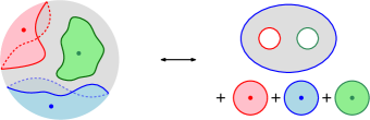
Figure 1: Cutting a quantum sphere and gluing a quantum pair of pants with quantum disks.

We call the non-simply connected surface obtained from cutting the quantum sphere a quantum pair of pants, since it is a natural LQG surface with the topology of a pair of pants. We also write the law of the quantum disk with one marked point as $\mathcal{M}_{1}^{\mathrm{disk}}(\gamma)$ where $\gamma$ represents the magnitude of the log singularity at the marked point. It is proved in [AHS17, Cer19, AHS21] that if we conformally embed a sample from $\mathrm{QS}_{3}$ on $\hat{\mathbbm{C}}=\mathbbm{C}\cup\infty$ with the three marked points located at $z_{1},z_{2},z_{3}$, then the corresponding variant of Gaussian free field is the so called Liouville field on the sphere [DKRV16, AHS21] with insertions of weight $\gamma$ at $z_{1},z_{2},z_{3}$. We set $(z_{1},z_{2},z_{3})=(0,1,e^{i\pi/3})$ and denote this field by $\mathrm{LF}_{\mathbbm{C}}^{\gamma,\gamma,\gamma}$. Similarly, if we embed $\mathcal{M}_{1}^{\mathrm{disk}}(\gamma)$ on $\mathbbm{H}$ with $i$ as the marked point and fix the remaining degree of freedom in the conformal embedding uniformly at random, then the resulting field is the Liouville field $\mathrm{LF}^{(\gamma,i)}_{\mathbbm{H}}$ on $\mathbbm{H}$ with a $\gamma$-insertion at $i$ [HRV18, ARS21]. (Here for the simplicity of presentation we have omitted a $\gamma$-dependent constant in front of $\mathrm{LF}$.)

Reversing the sphere-cutting procedure above, we conclude that if a quantum pair of pants and three quantum disks with interior marked points are glued together and conformally embedded to $(\mathbbm{C},0,1,e^{i\pi/3})$ (see Figure 1), then the law of the resulting field is $\mathrm{LF}_{\mathbbm{C}}^{\gamma,\gamma,\gamma}$. This gluing procedure is an example of conformal welding which we review in Section 2.4. In [ARS21], with Remy we considered a generalization $\mathcal{M}_{1}^{\mathrm{disk}}(\alpha)$ of $\mathcal{M}_{1}^{\mathrm{disk}}(\gamma)$ for generic $\alpha\in\mathbbm{R}$ such that if a sample from $\mathcal{M}_{1}^{\mathrm{disk}}(\alpha)$ is embedded to $(\mathbbm{H},i)$ as in the previous paragraph, then the law of the resulting random field is $\mathrm{LF}_{\mathbbm{H}}^{(\alpha,i)}$. Our key observation is that if we glue together the quantum pair of pants with three samples from $\mathcal{M}_{1}^{\mathrm{disk}}(\alpha_{i})$ with $i=1,2,3$, and conformally embed the spherical surface to $(\mathbbm{C},0,1,e^{i\pi/3})$, then the law of the resulting field is ${C^{\operatorname{CLE}}_{\kappa}(\lambda_{1},\lambda_{2},\lambda_{3})}\mathrm{LF}_{\mathbbm{C}}^{\alpha_{1},\alpha_{2},\alpha_{3}}$ where ${C^{\operatorname{CLE}}_{\kappa}(\lambda_{1},\lambda_{2},\lambda_{3})}$ is as in Theorem 1.2. Let $A$ be the total quantum area of the resulting sphere after gluing. Then using the relation between $\mathrm{LF}_{\mathbbm{C}}^{\alpha_{1},\alpha_{2},\alpha_{3}}$ and the DOZZ formula as we recall in Theorem 2.6, we can conclude that the average of $e^{-A}$ equals ${C^{\operatorname{CLE}}_{\kappa}(\lambda_{1},\lambda_{2},\lambda_{3})}\times\frac{1}{2}C^{\mathrm{DOZZ}}_{\gamma}(\alpha_{1},\alpha_{2},\alpha_{3})$.

In order to get ${C^{\operatorname{CLE}}_{\kappa}(\lambda_{1},\lambda_{2},\lambda_{3})}$, it suffices to compute the average of $e^{-A}$ in terms of the quantum pair of pants and $\mathcal{M}_{1}^{\mathrm{disk}}(\alpha_{i})$. The area and length distribution for $\mathcal{M}_{1}^{\mathrm{disk}}(\alpha)$ is encoded by the so-called FZZ formula for LCFT, which we proved in [ARS21] with Remy. A substantial effort of this paper is devoted to computing the joint area and length distribution for the quantum pair of pants. Two key ingredients of our computation are: 1. the LQG lengths of outermost loops of a CLE on a quantum disk can be described by the jump sizes of a stable Levy process; 2. the surfaces encircled by these outermost loops are independent quantum disks given their boundary lengths. These facts are consistent with the assertion that CLE coupled with LQG describes the scaling limit of $O(n)$-loop model decorated random planar maps, and are extracted from [MSW20, CCM20, BBCK18] as we summarize in Section 2.5. As an intermediate step towards solving the quantum pair of pants, we compute the joint length and area distribution of the quantum annulus, which is the LQG surface between the disk boundary and an outermost loop for CLE on a quantum disk.

The loop lengths distribution of $\operatorname{CLE}$ on quantum disk crucially relies on the mating of trees theory for LQG coupled with SLE and CLE, which was developed by Duplantier, Miller and Sheffield [DMS14]; see [GHS19] for a survey. The idea of using conformal welding, mating of trees, and LCFT to get integrable results is also applied to a variant of SLE called chordal $\operatorname{SLE}_{\kappa}(\rho_{-};\rho_{+})$ in our recent work with Holden [AHS21]. Moreover, conformal welding and mating of trees are used in our recent proof with Remy [ARS21] of the FZZ formula. In the next subsection we present yet another result based on these ideas.

1.3 SLE loop measure and the electrical thickness

For $\kappa\in(0,4]$, Kontsevich and Suhov [KS07] conjectured that up to a multiplicative constant there exists a unique measure on simple loops on $\hat{\mathbbm{C}}$ with conformal symmetry and a certain restriction property indexed by $\kappa$. This conjecture is inspired by Malliavin’s work [Mal99]. We call loop measures satisfying this conjecture a Malliavin-Kontsevich-Suhov (MKS) loop measure. For $\kappa=\frac{8}{3}$, the existence and uniqueness of the MKS loop measure was proved by Werner [Wer08] where the construction is via the Brownian loop measure.

Kemppainen and Werner [KW16] introduced the loop intensity measure of simple CLE, which gives an example of an MKS loop measure for $\kappa\in(\frac{8}{3},4]$. Let $\Gamma$ be a full-plane $\operatorname{CLE}_{\kappa}$ with $\kappa\in(\frac{8}{3},4]$. Let $\eta$ be a loop chosen from the counting measure over the set of loops in $\Gamma$. The loop intensity measure $\widetilde{\operatorname{SLE}}_{\kappa}^{\mathrm{loop}}$ for $\operatorname{CLE}_{\kappa}$ is the distribution of $\eta$, which is an infinite measure on simple loops. By the conformal invariance of $\operatorname{CLE}_{\kappa}$, the measure $\widetilde{\operatorname{SLE}}_{\kappa}^{\mathrm{loop}}$ is conformally invariant. Recently, for all $\kappa\in(0,4]$, Zhan [Zha21] constructed a MKS loop measure $\operatorname{SLE}^{\mathrm{loop}}_{\kappa}$, which we will recall in Section 2.4. As explained to us by Werner, the measures $\operatorname{SLE}^{\mathrm{loop}}_{\kappa}$ and $\widetilde{\operatorname{SLE}}_{\kappa}^{\mathrm{loop}}$ agree up to a multiplicative constant, namely, for each $\kappa\in(\frac{8}{3},4]$, there exists $C\in(0,\infty)$ such that $\widetilde{\operatorname{SLE}}_{\kappa}^{\mathrm{loop}}=C\operatorname{SLE}_{\kappa}^{\mathrm{loop}}$. We state this as Theorem 2.18 and include a proof that is essentially from [KW16].

Although the SLE loop measure is infinite, we can define a probability measure that describes the law of its shape modulo scaling. One way to express this shape measure is the following. Given a simple loop on $\mathbbm{C}$ that surrounds $0$, let $R_{\eta}=\inf\{|z|:z\in\eta\}$ and $\hat{\eta}=\{z:R_{\eta}z\in\eta\}$. Namely, $\hat{\eta}$ is the rescaling of $\eta$ such that $\hat{\eta}$ surrounds $\mathbbm{D}$ and touches $\partial\mathbbm{D}$. Now suppose $\eta$ is sampled from $\operatorname{SLE}_{\kappa}^{\mathrm{loop}}$ restricted to the event that $\eta$ surrounds $0$. By the conformal invariance of $\operatorname{SLE}_{\kappa}^{\mathrm{loop}}$, the law of $\log R_{\eta}$ is translation invariant on $\mathbbm{R}$, hence a constant multiple of the Lebesgue measure. Moreover, the conditional law of $\hat{\eta}$ conditioning on $R_{\eta}$ does not depend on the value of $R_{\eta}$, which gives a probability measure on loops that surround $\mathbbm{D}$ and touch $\partial\mathbbm{D}$. We denote this probability measure by $\mathcal{L}_{\kappa}$ and call it the shape measure of $\operatorname{SLE}_{\kappa}^{\mathrm{loop}}$.

Our next result is an exact formula for the so-called electrical thickness for a sample from $\mathcal{L}_{\kappa}$.

Theorem 1.3.

For $\kappa\in(0,4]$, let $\eta$ be sampled from $\mathcal{L}_{\kappa}$. Let $\bar{\eta}$ be the image of $\eta$ under the inversion map $z\mapsto z^{-1}$. Let $\vartheta(\eta)=-\log\mathrm{CR}(\eta,0)-\log\mathrm{CR}(\bar{\eta},0)$. Then $\mathbbm{E}[e^{\lambda\vartheta(\eta)}]<\infty$ if and only if $\lambda<1-\frac{\kappa}{8}$. Moreover,

$$\mathbbm{E}[e^{\lambda\vartheta(\eta)}]=\frac{\sin(\pi(1-\kappa/4))}{\pi(1-\kappa/4)}\frac{\pi\sqrt{(1-\kappa/4)^{2}+\lambda\kappa/2}}{\sin(\pi\sqrt{(1-\kappa/4)^{2}+\lambda\kappa/2})}\quad\text{ for }\lambda<1-\frac{\kappa}{8}.$$ (1.5)

We call $\theta(\eta)$ the electrical thickness of $\eta$. It only depends on the shape of $\eta$. It is non-negative and equals $0$ if and only if the loop is a circle around $0$. This quantity was introduced by Kenyon and Wilson [KW04] as a way of describing how much the shape of a loop differs from a circle. Viewing the complex plane as a homogeneous electrical material, the electrical thickness measures the net change in the effective resistance between $0$ and $\infty$ when the loop $\eta$ becomes a perfect conductor.

Theorem 1.3 settles a conjecture of Kenyon and Wilson on the electrical thickness of CLE loops for $\kappa\in(\frac{8}{3},4]$. Consider the shape measure $\widetilde{\mathcal{L}}_{\kappa}$ of $\widetilde{\operatorname{SLE}}_{\kappa}^{\mathrm{loop}}$ defined in the same way as $\mathcal{L}_{\kappa}$. Then we must have $\mathcal{L}_{\kappa}=\widetilde{\mathcal{L}}_{\kappa}$. Let $(\eta_{n})_{n\geq 1}$ be the sequence of loops of a $\operatorname{CLE}_{\kappa}$ on the unit disk surrounding the origin, ordered such that $\eta_{n}$ surrounds $\eta_{n+1}$. It is proved in [KW16] that the law of the rescaled loop $\hat{\eta}_{n}$ converges weakly to $\widetilde{\mathcal{L}}_{\kappa}$. Since $\vartheta(\eta_{n})=\vartheta(\hat{\eta}_{n})$, we see that $\lim_{n\to\infty}\mathbbm{E}[e^{\lambda\vartheta(\eta_{n})}]$ equals $\mathbbm{E}[e^{\lambda\vartheta(\eta)}]$ in Theorem 1.3. Kenyon and Wilson [KW04] conjectured a formula for $\lim_{n\to\infty}\mathbbm{E}[e^{\lambda\vartheta(\eta_{n})}]$, as recorded in [SSW09, Eq (14)]. Their formula agrees with the right hand of (1.5) after $\kappa$ is replaced by $16/\kappa$. Thus our Theorem 1.3 shows that the conjectural formula is false but only off by this flip. The conjecture was made for the entire CLE range $\kappa\in(\frac{8}{3},8)$. In a subsequent paper we will prove that $\lim_{n\to\infty}\mathbbm{E}[e^{\lambda\vartheta(\eta_{n})}]$ converges to the right hand side of (1.5) for $\kappa\in(4,8)$ as well.

Our proof of Theorem 1.3 also relies on the conformal welding of LQG surfaces and the integrability of LCFT. This time we glue together two quantum disks, each of which has an interior point, to obtain a two-pointed quantum sphere with a loop separating them. It was shown by us and Holden in [AHS21] that the law of the resulting loop is $\operatorname{SLE}_{\kappa}^{\mathrm{loop}}$. Using this conformal welding result and a similar strategy as outlined in Section 1.2, we can express $\mathbbm{E}[e^{\lambda\vartheta(\eta)}]$ in Theorem 1.3 using the FZZ formula and the reflection coefficient for LCFT on the sphere [KRV17, RV19]. A new difficulty arises as the measure $\operatorname{SLE}_{\kappa}^{\mathrm{loop}}$ is infinite, even after restricting to loops that separate $0$ and $\infty$. Overcoming this is the technical bulk of our proof of Theorem 1.3 in Section 6.

1.4 Outlook and perspectives

One natural direction to explore after Theorem 1.2 is to compute higher order correlators in two dimensional random cluster and loop models using the so-called conformal bootstrap method in conformal field theory (CFT) [BPZ84]. With the DOZZ formula established in [KRV17] as an input, the conformal bootstrap for the LCFT was recently carried out in [GKRV20]. However, the CFTs corresponding to random cluster and loop models are less understood than LCFT, and remain an active topic in physics; see e.g. [PRS16, LJS19, HJS20]. Another natural direction to explore is to use the interplay between different types of integrability of SLE, CLE, LQG, LCFT to obtain results that are inaccessible within a single framework. The potential of this program was also demonstrated in our recent papers [AHS21] with Holden and [ARS21] with Remy. We refer to the introductions of those papers for more results and problems in this direction.

We conclude the introduction with three problems that we will pursue in subsequent works and three concrete open questions.

1. In a forthcoming paper we will extend our method to prove Theorems 1.2 and 1.3 for $\kappa\in(4,8)$ using the coupling of $\operatorname{CLE}_{\kappa}$ with $\sqrt{16/\kappa}$-LQG from [MSW21].

2. In the random cluster models, the connectivity functions $P_{n}(x_{1},\cdots,x_{n})$ are given by the probabilities that $n$ points belong to the same cluster [KSZ06]. Delfino and Vici [DV11] conjectured that at criticality in the continuum limit, the ratio $P_{3}(x_{1},x_{2},x_{3})/\sqrt{P_{2}(x_{1},x_{2})P_{2}(x_{1},x_{3})P_{2}(x_{2},x_{3})}$ converges to a universal constant only depending on $\operatorname{CLE}_{\kappa}$, which can be expressed by the imaginary DOZZ formula at a special value. In particular, for percolation this constant is $\approx 1.022$. See[ZSK11, PSVD13] for numercial verifications of this conjecture. We plan to prove the conjectural formula for CLE based on results and methods in our paper.

3. LQG surfaces with non-simply connected topology such as the quantum pair of pants and quantum annulus mentioned in Section 1.2 are crucial to our proof of Theorem 1.2. We plan to establish two general facts on non-simply connected LQG surfaces which are supposed to be the scaling limit of natural decorated random planar maps with the same topology. First, conditioned on their conformal structure, their random fields are Liouville fields. Second, they behave nicely under conformal welding. Beyond their intrinsic interests, we believe that proving these results will be instrumental to answering Questions 1.5 and 1.6 below.

Question 1.4.

Can one prove Theorem 1.2 without relying on LQG? The imaginary DOZZ formula can be characterized by Teschner’s shift relations for DOZZ formula [Tes95] with imaginary shifts. One natural idea is to use the strategy in [KRV17] for the proof of the DOZZ formula for LCFT, which is based on CFT ideas including the BPZ equation and operator product expansion. Carrying this out for CLE would represent a big step towards computing higher order correlation functions.

Question 1.5.

What is the law of the random modulus for our quantum annulus conditioning on its two boundary lengths? This question is naturally related to the extremal distance between CLE loops, which is well understood for $\operatorname{CLE}_{4}$ [ALS20] using the level line coupling with Gaussian free field, but not known for $\kappa\neq 4$.

Question 1.6.

Can the imaginary DOZZ formula in (1.3) for $\kappa\in(0,8/3]$ be realized as an $\operatorname{SLE}_{\kappa}$ observable? For Theorem 1.3, although it was originally only considered for $\operatorname{CLE}_{\kappa}$ [SSW09], we have shown that it holds for the $\operatorname{SLE}_{\kappa}$ loop when $\kappa\in(0,8/3]$. Thus one natural idea is to construct a measure on triples of loop defined via the $\operatorname{SLE}_{\kappa}$ loop and consider their conformal radii.

Organization of the paper. In Section 2, we provide background on LQG, LCFT and their coupling with SLE and CLE. In Section 3 we introduce the quantum annulus and pair of pants, and prove the needed conformal welding results. In Section 4 we compute their area and length distributions. In Section 5 we carry out the outline in Section 1.2 to prove Theorem 1.2. In Section 6 we prove Theorem 1.3.

Acknowledgements. We are grateful to Wendelin Werner for explaining to us that Theorem 2.18 was implicitly proved in [KW16]. We thank Nicolas Curien, Nina Holden, Rick Kenyon, Matthis Lehmkuehler, and Scott Sheffield for helpful discussions. We also thank Ewain Gwynne and Dapeng Zhan for helpful comments on an earlier version of this paper. M.A. was partially supported by NSF grant DMS-1712862. X.S. was supported by the NSF grant DMS-2027986 and the NSF Career grant DMS-2046514.

2 Preliminaries

We assume basic familiarity with SLE and CLE in the simple curve regime and refer to [SW12] for more background. In this section, we review the inputs for our proofs from Liouville quantum gravity, Liouville conformal field theory, and their interplay with SLE and CLE.

2.1 Measure theoretic background

We will frequently consider infinite measures and extend the probability terminology to this setting. In particular, suppose $M$ is a $\sigma$-finite measure on a measurable space $(\Omega,\mathcal{F})$. Suppose $X:(\Omega,\mathcal{F})\rightarrow(E,\mathcal{E})$ is an $\mathcal{F}$-measurable function taking values in $(E,\mathcal{E})$. Then we say that $X$ is a random variable on $(\Omega,\mathcal{F})$ and call the pushforward measure $M_{X}=X_{*}M$ on $(E,\sigma(X))$ the law of $X$. We say that $X$ is sampled from $M_{X}$. We also write the integral $\int f(x)M_{X}(dx)$ as $M_{X}[f]$ for simplicity. For a finite measure $M$, we write $|M|$ as its total mass and write $M^{\#}=|M|^{-1}M$ as the probability measure proportional to $M$.

Given $(\Omega,\mathcal{F},M)$ as above, let $X:(\Omega,\mathcal{F})\rightarrow(E,\mathcal{E})$ and $Y:(\Omega,\mathcal{F})\rightarrow(E^{\prime},\mathcal{E}^{\prime})$ be two random variables. A family of probability measures $\{\mathbbm{P}(\cdot|e):e\in E\}$ on $(E^{\prime},\mathcal{E}^{\prime})$ is called the (regular) conditional law of $Y$ given $X$ if for each $A\in\sigma(Y)$, $\mathbbm{P}(A|\cdot)$ is measurable on $(E,\mathcal{E})$ and

$$M[Y\in A,X\in B]=\int_{B}\mathbbm{P}(A|e)\,dM_{X}\textrm{ for each }A\in\mathcal{E}^{\prime}\textrm{ and }B\in\mathcal{E}.$$

We also need the concept of disintegration in the case $(E,\mathcal{E})=\mathbbm{R}^{n}$ for a positive integer $n$.

Definition 2.1 (Disintegration).

Let $M$ be a measure on a measurable space $(\Omega,\mathcal{F})$. Let $X:\Omega\rightarrow\mathbbm{R}^{n}$ be a measurable function with respect to $\mathcal{F}$, where $\mathbbm{R}^{n}$ is endowed with the Borel $\sigma$-algebra. A family of measures $\{M_{x}:x\in\mathbbm{R}^{n}\}$ on $(\Omega,\mathcal{F})$ is called a disintegration of $M$ over $X$ if for each set $A\in\mathcal{F}$, the function $x\mapsto M_{x}(A)$ is Borel measurable, and

$$\int_{A}f(X)\,dM=\int_{\mathbbm{R}^{n}}f(x)M_{x}(A)\,d^{n}x\textrm{ for each non-negative measurable function }f\textrm{on }\mathbbm{R}^{n}.$$ (2.1)

When (2.1) holds, we simply write $M=\int_{\mathbbm{R}^{n}}M_{x}\,d^{n}x$.

Lemma 2.2 (Existence and uniqueness of disintegration).

In the setting of Definition 2.1, suppose $M$ is $\sigma$-finite and $X$ satisfies $M[X\in B]=0$ for each Borel set $B\subset\mathbbm{R}^{n}$ with zero Lebesgue measure. Then the disintegration of $M$ over $X$ exists. Moreover if $\{M_{x}:x\in\mathbbm{R}^{n}\}$ and $\{M^{\prime}_{x}:x\in\mathbbm{R}^{n}\}$ are two disintegrations of $M$ over $X$, then $M_{x}=M^{\prime}_{x}$ for almost every $x$.

Proof.

When $M$ is a probability measure, since the law $M_{X}$ of $X$ is absolutely continuous with respect to the Lebesgue measure, we can and must set $|M_{x}|$ to be the Radon-Nykodim derivative between the two measures. Since $\mathbbm{R}^{n}$ is complete and separable, we can and must set $\{M_{x}^{\#}\}$ to be the regular conditional probability of $M$ given $X$; see e.g. [Dur10, Chapter 4.1.3] for more detail on regular conditional probability. This gives the desired existence and uniqueness of $M_{x}=|M_{x}|M_{x}^{\#}$. By scaling this gives Lemma 2.2 when $M$ is finite. If $M$ is infinite, consider $\Omega_{n}\uparrow\Omega$ with $M(\Omega_{n})<\infty$. Applying Lemma 2.2 to $M|_{\Omega_{n}}$ and then sending $n\to\infty$ give the general result. ∎

2.2 Liouville quantum gravity and Liouville conformal field theory

In this section we review the precise definitions of some $\gamma$-LQG surfaces and Liouville fields mentioned in Section 1.2. For more background, we refer to [GHS19, Var17] and references therein, as well as the preliminary sections in [AHS21, ARS21].

2.2.1 Gaussian free field, Liouville field, and the DOZZ formula

Let $\mathcal{X}$ be the complex plane $\mathbbm{C}$ or the upper half plane $\mathbbm{H}$. Suppose $\mathcal{X}$ is endowed with a smooth metric $g$ such that the metric completion of $(\mathcal{X},g)$ is a compact Riemannian manifold. (We will not distinguish $\mathcal{X}$ with its compactification for notional simplicity.) Let $H^{1}(\mathcal{X})$ be the Sobolev space whose norm is the sum of the $L^{2}$-norm with respect to $(\mathcal{X},g)$ and the Dirichlet energy. Let $H^{-1}(\mathcal{X})$ be the dual space of $H^{1}(\mathcal{X})$.

We now recall two basic variants of the Gaussian free field (GFF). Consider the two functions

$$G_{\mathbbm{H}}(z,w) =-\log|z-w|-\log|z-\overline{w}|+2\log|z|_{+}+2\log|w|_{+}\quad z,w\in\mathbbm{H},$$

$$G_{\mathbbm{C}}(z,w) =-\log|z-w|+\log|z|_{+}+\log|w|_{+}\quad z,w\in\mathbbm{C}.$$

Here $|z|_{+}:=\max\{|z|,1\}$ so that $\log|z|_{+}=\max\{\log|z|,0\}$. Let $h_{\mathcal{X}}$ be a random element in $H^{-1}(\mathcal{X})$ such that $(h_{\mathcal{X}},f)$ is a centered Gaussian with variance $\int f(z)G_{\mathcal{X}}(z,w)f(w)\,d^{2}z\,d^{2}w$ for each $f\in H^{1}(\mathcal{X})$. Then $h_{\mathbbm{C}}$ is a whole plane GFF and $h_{\mathbbm{H}}$ is a free-boundary GFF on $\mathbbm{H}$, both of which are normalized to have mean zero along $\{z\in\mathcal{X}:|z|=1\}$. We denote the law of $h_{\mathcal{X}}$ by $P_{\mathcal{X}}$.

We now review the Liouville fields on $\mathbbm{C}$ and $\mathbbm{H}$ following [AHS21, Section 2.2].

Definition 2.3.

Suppose $(h,\mathbf{c})$ is sampled from $P_{\mathbbm{C}}\times[e^{-2Qc}dc]$ and set $\phi=h(z)-2Q\log|z|_{+}+\mathbf{c}$. Then we write $\mathrm{LF}_{\mathbbm{C}}$ as the law of $\phi$ and call a sample from $\mathrm{LF}_{\mathbbm{C}}$ a Liouville field on $\mathbbm{C}$.

Suppose $(h,\mathbf{c})$ is sampled from $P_{\mathbbm{H}}\times[e^{-Qc}dc]$ and set $\phi=h(z)-2Q\log|z|_{+}+\mathbf{c}$. Then we write $\mathrm{LF}_{\mathbbm{H}}$ as the law of $\phi$ and call a sample from $\mathrm{LF}_{\mathbbm{H}}$ a Liouville field on $\mathbbm{H}$.

We also need the following Liouville fields with insertions.

Definition 2.4.

Let $(\alpha_{i},z_{i})\in\mathbbm{R}\times\mathbbm{C}$ for $i=1,\dots,m$, where $m\geq 1$ and the $z_{i}$’s are distinct. Let $(h,\mathbf{c})$ be sampled from $C_{\mathbbm{C}}^{(\alpha_{i},z_{i})_{i}}P_{\mathbbm{C}}\times[e^{(\sum_{i}\alpha_{i}-2Q)c}dc]$ where

$$C_{\mathbbm{C}}^{(\alpha_{i},z_{i})_{i}}=\prod_{i=1}^{m}|z_{i}|_{+}^{-\alpha_{i}(2Q-\alpha_{i})}e^{\sum_{i<j}\alpha_{i}\alpha_{j}G_{\mathbbm{C}}(z_{i},z_{j})}.$$

Let $\phi(z)=h(z)-2Q\log|z|_{+}+\sum_{i=1}^{m}\alpha_{i}G_{\mathbbm{C}}(z,z_{i})+\mathbf{c}$. We write $\mathrm{LF}_{\mathbbm{C}}^{(\alpha_{i},z_{i})_{i}}$ for the law of $\phi$ and call a sample from $\mathrm{LF}_{\mathbbm{C}}^{(\alpha_{i},z_{i})_{i}}$ a Liouville field on $\mathbbm{C}$ with insertions $(\alpha_{i},z_{i})_{1\leq i\leq m}$.

Definition 2.5.

For $\alpha\in\mathbbm{R}$ and $z_{0}\in\mathbbm{H}$, let $(h,\mathbf{c})$ be sampled from $(2\operatorname{Im}z_{0})^{-\alpha^{2}/2}|z_{0}|_{+}^{-2\alpha(Q-\alpha)}P_{\mathbbm{H}}\times[e^{(\alpha-Q)c}dc]$. Let $\phi(z)=h(z)-2Q\log|z|_{+}+\alpha G_{\mathbbm{H}}(z,z_{0})+\mathbf{c}$. We write $\mathrm{LF}_{\mathbbm{H}}^{(\alpha,z_{0})}$ for the law of $\phi$ and call a sample from $\mathrm{LF}_{\mathbbm{H}}^{(\alpha,z_{0})}$ a Liouville field on $\mathbbm{H}$ with insertion $(\alpha,z_{0})$.

The measure $\mathrm{LF}_{\mathbbm{C}}^{(\alpha_{i},z_{i})_{i}}$ from Definition 2.4 formally equals $\prod_{i=1}^{m}e^{\alpha_{i}\phi(z_{i})}\mathrm{LF}_{\mathbbm{C}}$. This can be made rigorous by a regularization and limiting procedure; see [AHS21, Lemma 2.8]. In the same manner we have $\mathrm{LF}_{\mathbbm{H}}^{(\alpha,z_{0})}=e^{\alpha\phi(z_{0})}\mathrm{LF}_{\mathbbm{H}}$; see [ARS21, Lemma 2.2].

Fix $\gamma\in(0,2)$, we now recall the quantum area and quantum length measures in $\gamma$-LQG. Suppose $h$ is a GFF sampled from $P_{\mathcal{X}}$ for $\mathcal{X}=\mathbbm{C}$ or $\mathbbm{H}$. For $\varepsilon>0$ and $z\in\mathcal{X}\cup\partial\mathcal{X}$, we write $h_{\varepsilon}(z)$ for the average of $h$ on $\{w\in\mathcal{X}\>:\>|w-z|=\varepsilon\}$, and define the random measure $\mu_{h}^{\varepsilon}:=\varepsilon^{\gamma^{2}/2}e^{\gamma h_{\varepsilon}(z)}d^{2}z$ on $\mathcal{X}$, where $d^{2}z$ is Lebesgue measure on $\mathcal{X}$. Almost surely, as $\varepsilon\to 0$, the measures $\mu_{h}^{\varepsilon}$ converge weakly to a limiting measure $\mu_{h}$ called the quantum area measure [DS11, SW16]. For $\mathcal{X}=\mathbbm{H}$, we define the quantum boundary length measure $\nu_{h}:=\lim_{\varepsilon\to 0}\varepsilon^{\gamma^{2}/4}e^{\frac{\gamma}{2}h_{\varepsilon}(x)}dx$. The definition of quantum area and boundary length can clearly be extended to other variants of GFF such as the Liouville fields, possibly with insertions.

We now review the DOZZ formula for the structure constant of LCFT.

Theorem 2.6 ([KRV17]).

Suppose $\alpha_{1},\alpha_{2},\alpha_{3}$ satisfy the Seiberg bounds

$$\sum_{i=1}^{3}\alpha_{i}>2Q,\qquad\textrm{and}\qquad\alpha_{i}<Q\text{ for }i=1,2,3.$$ (2.2)

Let $(z_{1},z_{2},z_{3})=(0,1,e^{i\pi/3})$. Then with $\mu>0$ and $C^{\mathrm{DOZZ}}_{\gamma}(\alpha_{1},\alpha_{2},\alpha_{3})$ defined in (1.2), we have

$$\mathrm{LF}_{\mathbbm{C}}^{(\alpha_{i},z_{i})_{i}}[e^{-\mu\mu_{\phi}(\mathbbm{C})}]=\frac{1}{2}C^{\mathrm{DOZZ}}_{\gamma}(\alpha_{1},\alpha_{2},\alpha_{3})\mu^{\frac{2Q-\alpha_{1}-\alpha_{2}-\alpha_{3}}{\gamma}}.$$

Here, the Seiberg bounds ensure that $\mathrm{LF}_{\mathbbm{C}}^{(\alpha_{i},z_{i})_{i}}[e^{-\mu\mu_{\phi}(\mathbbm{C})}]$ is finite, and the points $z_{1},z_{2},z_{3}$ are chosen such that $|z_{1}-z_{2}|=|z_{2}-z_{3}|=|z_{3}-z_{1}|=1$ for convenience. Moreover, as remarked in  [KRV17, Footnote 6], the factor $\frac{1}{2}$ is included to match with the convention from physics.

2.2.2 Quantum sphere

A quantum surface is an equivalence class of pairs $(D,h)$ where $D$ is a planar domain and $h$ is a generalized function on $D$. For $\gamma\in(0,2)$, we say that $(D,h)\sim_{\gamma}(\widetilde{D},\widetilde{h})$ if there is a conformal map $\psi:\widetilde{D}\to D$ such that

$$\widetilde{h}=h\circ\psi+Q\log|\psi^{\prime}|.$$ (2.3)

We write $(D,h)/{\sim_{\gamma}}$ as the quantum surface corresponding to $(D,h)$. An embedding of a quantum surface is a choice of its representative. Both the notions of quantum area and quantum length measures are intrinsic to the quantum surface [DS11, SW16].

We can also consider quantum surfaces decorated with other structures. For example, let $n\in\mathbbm{N}$ and $\mathcal{I}$ be an at most countable index set, consider tuples $(D,h,(\eta_{i})_{i\in\mathcal{I}},z_{1},\cdots,z_{n})$ such that $D$ is a domain, $h$ is a distribution on $D$, $\eta_{i}$ are loops on $D$ and $z_{i}\in D\cup\partial D$. We say that

$$(D,h,(\eta_{i})_{i\in\mathcal{I}},z_{1},\cdots,z_{n})\sim_{\gamma}(\widetilde{D},\widetilde{h},(\widetilde{\eta}_{i})_{i\in\mathcal{I}},\widetilde{z}_{1},\cdots,\widetilde{z}_{n})$$

if there is a conformal map $\psi:\widetilde{D}\to D$ such that (2.3) holds, $\psi(\widetilde{z}_{i})=z_{i}$ for all $1\leq i\leq n$, and $\psi\circ\widetilde{\eta}_{i}=\eta_{i}$ for all $i\in\mathcal{I}$. We call an equivalence class defined through ${\sim_{\gamma}}$ a decorated quantum surface, and call a choice of its representative an embedding.

We now recall the two-pointed quantum sphere defined in [DMS14] following the presentation of [AHS20, AHS21]. Consider the horizontal cylinder $\mathcal{C}$ obtained from $\mathbbm{R}\times[0,2\pi]$ by identifying $(x,0)\sim(x,2\pi)$. Let $h_{\mathcal{C}}(z)=h_{\mathbbm{C}}(e^{z})$ for $z\in\mathcal{C}$ where $h_{\mathbbm{C}}$ is sampled from $P_{\mathbbm{C}}$. We call $h_{\mathcal{C}}$ the GFF on $\mathcal{C}$ normalized to have mean zero on the circle $\{\operatorname{Re}z=0\}\cap\mathcal{C}$. The field $h_{\mathcal{C}}$ can be written as $h_{\mathcal{C}}=h^{\operatorname{1}}_{\mathcal{C}}+h^{2}_{\mathcal{C}}$, where $h^{\operatorname{1}}_{\mathcal{C}}$ is constant on vertical circles $\{\operatorname{Re}z=u\}\cap\mathcal{C}$ for each $u\in\mathbbm{R}$, and $h^{2}_{\mathcal{C}}$ has mean zero on all such circles. We call $h^{2}_{\mathcal{C}}$ the lateral component of the GFF on $\mathcal{C}$.

Definition 2.7.

For $\gamma\in(0,2)$, let $(B_{s})_{s\geq 0}$ be a standard Brownian motion conditioned on $B_{s}-(Q-\gamma)s<0$ for all $s>0$, and let $(\widetilde{B}_{s})_{s\geq 0}$ be an independent copy of $(B_{s})_{s\geq 0}$. Let

$$Y_{t}=\mathopen{}\mathclose{{}\left\{\begin{array}[]{ll}B_{t}-(Q-\gamma)t&\mbox{if }t\geq 0\\ \widetilde{B}_{-t}+(Q-\gamma)t&\mbox{if }t<0\end{array}}\right..$$

Let $h^{1}(z)=Y_{\operatorname{Re}z}$ for each $z\in\mathcal{C}$. Let $h^{2}_{\mathcal{C}}$ be independent of $h^{1}$ and have the law of the lateral component of the GFF on $\mathcal{C}$. Let $\hat{h}=h^{1}+h^{2}_{\mathcal{C}}$. Let $\mathbf{c}\in\mathbbm{R}$ be sampled from $\frac{\gamma}{2}e^{2(\gamma-Q)c}dc$ independently of $\hat{h}$ and set $h=\hat{h}+\mathbf{c}$. Let $\mathrm{QS}_{2}$ be the infinite measure describing the law of the decorated quantum surface $(\mathcal{C},h,-\infty,+\infty)/{\sim_{\gamma}}$. We call a sample from $\mathrm{QS}_{2}$ a two-pointed quantum sphere.

The un-pointed and three-pointed quantum spheres are defined from $\mathrm{QS}_{2}$ as follows.

Definition 2.8.

Suppose the decorated quantum surface $(\mathcal{C},h,-\infty,+\infty)/{\sim_{\gamma}}$ is sampled from $\mu_{h}(\mathcal{C})^{-2}\mathrm{QS}_{2}$. We let $\mathrm{QS}$ be the law of the quantum surface $(\mathcal{C},h)/{\sim_{\gamma}}$. Suppose $(\mathcal{C},h,-\infty,+\infty)/{\sim_{\gamma}}$ is sampled from $\mu_{h}(\mathcal{C})\mathrm{QS}_{2}$. Let $z$ be sampled from the probability measure proportional to $\mu_{h}$. Then we let $\mathrm{QS}_{3}$ be the law of $(\mathcal{C},h,z,-\infty,+\infty)/{\sim_{\gamma}}$.

It is proved in [DMS14] that $\mathrm{QS}_{2}$ can be obtained from $\mathrm{QS}$ by adding two marked points according to the quantum area measure. Namely $\mathrm{QS}_{2}$ is invariant under re-sampling of its two marked points according to the quantum area. We can similarly define $\mathrm{QS}_{n}$ for $n\in\mathbbm{N}$ by adding quantum typical points to $\mathrm{QS}$ but we only need $\mathrm{QS}_{2}$ and $\mathrm{QS}_{3}$ in this paper.

It is shown in [AHS17, AHS21] that the embedding of $\mathrm{QS}_{3}$ in $\mathbbm{C}$ gives a Liouville field on $\mathbbm{C}$ with three $\gamma$-insertions modulo an explicit multiplicative constant.

Theorem 2.9 ([AHS21, Remark 2.30]).

Let $\phi$ be sampled from $\mathrm{LF}_{\mathbbm{C}}^{(\gamma,z_{1}),(\gamma,z_{2}),(\gamma,z_{3})}$ where $(z_{1},z_{2},z_{3})=(0,1,e^{i\pi/3})$. Then the law of the decorated quantum surface $(\mathbbm{C},\phi,z_{1},z_{2},z_{3})/{\sim_{\gamma}}$ is $\frac{2(Q-\gamma)^{2}}{\pi\gamma}\mathrm{QS}_{3}$.

2.2.3 Quantum disk and the FZZ formula

We first recall the law of the quantum boundary length under $\mathrm{LF}_{\mathbbm{H}}^{(\alpha,i)}$ obtained in [Rem20], following the presentation of [ARS21, Proposition 2.8].

Proposition 2.10 ([Rem20]).

For $\alpha>\frac{\gamma}{2}$, the law of the quantum length $\nu_{\phi}(\mathbbm{R})$ under $\mathrm{LF}_{\mathbbm{H}}^{(\alpha,i)}$ is

$$1_{\ell>0}\frac{2}{\gamma}2^{-\frac{\alpha^{2}}{2}}\overline{U}(\alpha)\ell^{\frac{2}{\gamma}(\alpha-Q)-1}\,d\ell$$

where

$$\overline{U}(\alpha)=\mathopen{}\mathclose{{}\left(\frac{2^{-\frac{\gamma\alpha}{2}}2\pi}{\Gamma(1-\frac{\gamma^{2}}{4})}}\right)^{\frac{2}{\gamma}(Q-\alpha)}\Gamma(\frac{\gamma\alpha}{2}-\frac{\gamma^{2}}{4}).$$ (2.4)

Let $\{\mathrm{LF}_{\mathbbm{H}}^{(\alpha,i)}(\ell):\ell\}$ be the disintegration of $\mathrm{LF}_{\mathbbm{H}}^{(\alpha,i)}$ over $\nu_{\phi}(\mathbbm{R})$. Namely for each non-negative measurable function $f$ on $(0,\infty)$ and $g$ on $H^{-1}(\mathbbm{H})$,

$$\mathrm{LF}_{\mathbbm{H}}^{(\alpha,i)}[f(\nu_{\phi}(\mathbbm{R}))g(\phi)]=\int_{0}^{\infty}f(\ell)\mathrm{LF}_{\mathbbm{H}}^{(\alpha,i)}(\ell)[g(\phi)]\,d\ell.$$ (2.5)

Although the general theory of disintegration only defines $\mathrm{LF}_{\mathbbm{H}}^{(\alpha,i)}(\ell)$ for almost every $\ell\in(0,\infty)$, the following lemma describes a canonical version of $\mathrm{LF}_{\mathbbm{H}}^{(\alpha,i)}(\ell)$ for every $\ell>0$.

Lemma 2.11 ([ARS21, Lemma 4.3]).

Let $h$ be a sample from $P_{\mathbbm{H}}$ and $\hat{h}(\cdot)=h(\cdot)-2Q\log\mathopen{}\mathclose{{}\left|\cdot}\right|_{+}+\alpha G_{\mathbbm{H}}(\cdot,i)$. Then the law of $\hat{h}+\frac{2}{\gamma}\log\frac{\ell}{\nu_{\widehat{h}}(\mathbbm{R})}$ under the reweighted measure $2^{-\alpha^{2}/2}\frac{2}{\gamma}\ell^{-1}\mathopen{}\mathclose{{}\left(\frac{\ell}{\nu_{\widehat{h}}(\mathbbm{R})}}\right)^{\frac{2}{\gamma}(\alpha-Q)}P_{\mathbbm{H}}$ is a version of the disintegration $\{\mathrm{LF}_{\mathbbm{H}}^{(\alpha,i)}(\ell):\ell>0\}$.

We now recall the quantum disk with one generic bulk insertion mentioned in Section 1.2.

Definition 2.12 ([ARS21]).

For $\ell>0$, we let $\mathcal{M}_{1}^{\mathrm{disk}}(\alpha;\ell)$ be the law of $(\mathbbm{H},\phi,i)/{\sim_{\gamma}}$ where $\phi$ is sampled from $\mathrm{LF}_{\mathbbm{H}}^{(\alpha,i)}(\ell)$.

The quantum disk with quantum typical marked points introduced in [DMS14] is defined similarly as $\mathrm{QS}_{n}$ in Definitions 2.7 and 2.8. We will not recall the definition from [DMS14] but recall that up to an explicit factor $\mathcal{M}_{1}^{\mathrm{disk}}(\gamma;\ell)$ is the law of the quantum disk with one-bulk typical point.

Theorem 2.13 ([ARS21, Theorem 3.4]).

Fix $\ell>0$. Let $\mathrm{QD}_{1,0}(\ell)$ be the law of the quantum disk with boundary length $\ell$ and with one interior marked point defined in [DMS14]. Then

$$\mathrm{QD}_{1,0}(\ell)=\frac{\gamma}{2\pi(Q-\gamma)^{2}}\mathcal{M}_{1}^{\mathrm{disk}}(\gamma;\ell).$$

Similarly as in the sphere case, other variants of quantum disks can be defined by adding or removing points from $\mathrm{QD}_{1,0}(\ell)$. We will need the following two variants.

Definition 2.14.

For $\ell>0$. Let $(D,h,z)/{\sim_{\gamma}}$ be sampled from $\mathrm{QD}_{1,0}(\ell)$. Then we let $\mathrm{QD}(\ell)$ be the law of $(D,h)/{\sim_{\gamma}}$ under $\mu_{h}(D)^{-1}\mathrm{QD}(\ell)$, Let $(D,h,z)/{\sim_{\gamma}}$ be sampled from $\ell\mathrm{QD}_{1,0}(\ell)$ and sample $p\in\partial D$ from the probability measure proportional to quantum boundary length measure. Then we define $\mathrm{QD}_{1,1}(\ell)$ to be the law of $(D,h,z,p)/{\sim_{\gamma}}$.

Remark 2.15.

By Proposition 2.10 and Theorem 2.13, the law of the quantum boundary length of $\mathrm{QD}_{1,0}$ (resp. $\mathrm{QD}$) is $C1_{\ell>0}\ell^{-\frac{4}{\gamma^{2}}}\,d\ell$ (resp. $C1_{\ell>0}\ell^{-\frac{4}{\gamma^{2}}-2}\,d\ell$) for some explicit constant $C$.

The FZZ formula is the analog of the DOZZ formula for $\mathrm{LF}^{(\alpha,i)}_{\mathbbm{H}}$ proposed in [FZZ00] and proved in [ARS21]. We record the most convenient form for our purpose, which uses the modified Bessel function of the second kind $K_{\nu}(x)$ [DLMF, Section 10.25]. One concrete representation of $K_{\nu}(x)$ in the range of our interest is the following [DLMF, (10.32.9)]:

$$K_{\nu}(x):=\int_{0}^{\infty}e^{-x\cosh t}\cosh(\nu t)\,dt\quad\text{ for }x>0\text{ and }\nu\in\mathbbm{R}.$$ (2.6)

Theorem 2.16 ([ARS21, Theorem 1.2, Proposition 4.19]).

For $\alpha\in(\frac{\gamma}{2},Q)$ and $\ell>0$, let $A$ be the quantum area of a sample from $\mathcal{M}_{1}^{\mathrm{disk}}(\alpha;\ell)$. The law of $A$ under $\mathcal{M}_{1}^{\mathrm{disk}}(\alpha;1)^{\#}$ (i.e. the probability measure proportional to $\mathcal{M}_{1}^{\mathrm{disk}}(\alpha;1)$) is the inverse gamma distribution with density

$$1_{x>0}\frac{(4\sin\frac{\pi\gamma^{2}}{4})^{-\frac{2}{\gamma}(Q-\alpha)}}{\Gamma(\frac{2}{\gamma}(Q-\alpha))}x^{-\frac{2}{\gamma}(Q-\alpha)-1}\exp\mathopen{}\mathclose{{}\left(-\frac{1}{4x\sin\frac{\pi\gamma^{2}}{4}}}\right)\,dx.$$

Moreover, recall $\overline{U}(\alpha)$ from in Proposition 2.10. Then for $\mu>0$ we have

$$\mathcal{M}_{1}^{\mathrm{disk}}(\alpha;\ell)[e^{-\mu A}]=\frac{2}{\gamma}2^{-\frac{\alpha^{2}}{2}}\overline{U}(\alpha)\ell^{-1}\frac{2}{\Gamma(\frac{2}{\gamma}(Q-\alpha))}\mathopen{}\mathclose{{}\left(\frac{1}{2}\sqrt{\frac{\mu}{\sin(\pi\gamma^{2}/4)}}}\right)^{\frac{2}{\gamma}(Q-\alpha)}K_{\frac{2}{\gamma}(Q-\alpha)}\mathopen{}\mathclose{{}\left(\ell\sqrt{\frac{\mu}{\sin(\pi\gamma^{2}/4)}}}\right).$$

We conclude with two integral identities on $K_{\nu}(x)$ that are used in our computation of ${C^{\operatorname{CLE}}_{\kappa}(\lambda_{1},\lambda_{2},\lambda_{3})}$. We provide their proofs in Appendix B.

$$\int_{0}^{\infty}\frac{1}{\sqrt{x}}e^{-cx}K_{\nu}(cx)\,dx=\frac{\pi^{3/2}}{\sqrt{2c}\cos(\pi\nu)}\quad\textrm{for }c>0\textrm{ and }\nu\in(-\frac{1}{2},\frac{1}{2}).$$ (2.7)

$$\iint_{0}^{\infty}\frac{1}{\sqrt{b}(b+1)}e^{-(b+1)x}K_{\nu}(bx)\,db\,dx=\frac{\pi^{2}}{2\cos(\pi\nu)\cos(\frac{1}{2}\pi\nu)}\quad\textrm{for }\nu\in(-\frac{1}{2},\frac{1}{2}).$$ (2.8)

2.3 Zhan’s SLE loop measure and the loop intensity measure of CLE

We first recall Zhan’s SLE loop measure $\operatorname{SLE}_{\kappa}^{\mathrm{loop}}$ from [Zha21] (see Theorem 4.2 there). It is a conformally invariant infinite measure on unrooted simple loops defined as follows. Given two distinct points $p,q\in\mathbbm{C}$ and $\kappa\in(0,4]$, the two-sided whole plane $\operatorname{SLE}_{\kappa}$, which we denote by $\operatorname{SLE}^{p\rightleftharpoons q}_{\kappa}$, is the probability measure on pairs of curves $(\eta_{1},\eta_{2})$ on $\mathbbm{C}$ connecting $p$ and $q$ where $\eta_{1}$ is a so-called whole-plane $\operatorname{SLE}_{\kappa}(2)$ from $p$ to $q$ and $\eta_{2}$ conditioned on $\eta_{1}$ is a chordal $\operatorname{SLE}_{\kappa}$ in $\widehat{\mathbbm{C}}\backslash\eta_{1}$. Forgetting $p$ and $q$, $\operatorname{SLE}^{p\rightleftharpoons q}_{\kappa}$ can be viewed as a measure on loops on $\mathbbm{C}$. Given a loop $\eta$ sampled from $\operatorname{SLE}^{p\rightleftharpoons q}_{\kappa}$, let $\operatorname{Cont}(\eta)$ be the $(1+\frac{\kappa}{8})$-dimensional Minkowski content, which exists a.s. by [LR15].

Definition 2.17.

Zhan’s SLE loop measure $\operatorname{SLE}^{\mathrm{loop}}_{\kappa}$ is the infinite measure on loops on $\mathbbm{C}$ given by

$$\operatorname{SLE}_{\kappa}^{\mathrm{loop}}:=\operatorname{Cont}(\eta)^{-2}\iint_{\mathbbm{C}\times\mathbbm{C}}|p-q|^{-2(1-\frac{\kappa}{8})}\operatorname{SLE}^{p\rightleftharpoons q}_{\kappa}(d\eta)\,d^{2}p\,d^{2}q.$$ (2.9)

We now recall the loop intensity measure of simple CLE introduced by Kemppainen and Werner [KW16]. Let $\Gamma$ be a full-plane $\operatorname{CLE}_{\kappa}$ with $\kappa\in(\frac{8}{3},4]$. Let $\eta$ be a loop chosen from the counting measure on the set of loops in $\Gamma$. The loop intensity measure $\widetilde{\operatorname{SLE}}_{\kappa}^{\mathrm{loop}}$ for $\operatorname{CLE}_{\kappa}$ is the distribution of $\eta$, which is an infinite measure on simple loops. By the conformal invariance of $\operatorname{CLE}_{\kappa}$, the measure $\widetilde{\operatorname{SLE}}_{\kappa}^{\mathrm{loop}}$ is conformally invariant.

As asserted in [Zha21, Footnote 1], for $\kappa\in(\frac{8}{3},4]$, the measures $\operatorname{SLE}^{\mathrm{loop}}_{\kappa}$ and $\widetilde{\operatorname{SLE}}_{\kappa}^{\mathrm{loop}}$ agree up to a multiplicative constant, which is consistent with the uniqueness conjecture on the MKS loop measure. Here we include a proof communicated to us by Werner, which is implicitly contained in [KW16]. Another proof was given in Section 4 of the first version of this paper on the arXiv.

Theorem 2.18.

For each $\kappa\in(\frac{8}{3},4]$, there exists $C\in(0,\infty)$ such that $\widetilde{\operatorname{SLE}}_{\kappa}^{\mathrm{loop}}=C\operatorname{SLE}_{\kappa}^{\mathrm{loop}}$.

Proof.

Let $\mu$ be the $\operatorname{SLE}_{\kappa}$ bubble measure on the upper half plane $\mathbbm{H}$ rooted at 0. This is an infinite measure supported on the space of loops in $\mathbbm{H}$ rooted at $0$; see [SW12, Theorem 1.2] for a definition. Let ${\mathrm{C}}$ be a circle on the plane. As proved in [KW16, Lemma 2], there exists a measure $\rho_{\mathrm{C}}$ on the space of triples $(D,p,\varphi)$ with $D\subset\widehat{\mathbbm{C}}$ simply-connected, $p\subset\partial D$, and $\varphi:\mathbbm{H}\to D$ a conformal map with $\varphi(0)=p$, such that the following holds. Let $(\rho_{\mathrm{C}}\otimes\mu)_{*}(d\eta)$ be the law of the loop $\eta=\varphi(\eta_{0})$ where $(D,p,\varphi,\eta_{0})$ is a tuple sampled from $\rho_{\mathrm{C}}\times\mu$. Then

$$1_{\eta\cap C\neq\emptyset}\widetilde{\operatorname{SLE}}_{\kappa}^{\mathrm{loop}}(d\eta)=1_{\eta\cap C\neq 0}(\rho_{\mathrm{C}}\otimes\mu)_{*}(d\eta).$$ (2.10)

Eq. (2.10) was proved below [KW16, Lemma 2], where the measure $\rho_{\mathrm{C}}$ is denoted by $\widetilde{\rho}^{z_{0},\varepsilon}$ while the center and radius of $\mathrm{C}$ are $z_{0}\cosh\varepsilon$ and $|z_{0}|\sinh\varepsilon$, respectively.

For $\varepsilon>0$ let $B_{\varepsilon}(z)=\{w:|w-z|<\varepsilon\}$ and $E_{\varepsilon}(z,\eta):=\{\eta\cap\partial B_{\varepsilon}(z)\neq\emptyset\}$. Let $d=1+\frac{\kappa}{8}$. Applying (2.10) with the circle $\mathrm{C}=\partial B_{\varepsilon}(z)$, we get

$$1_{E_{\varepsilon}(z,\eta)}\varepsilon^{d-2}\,\widetilde{\operatorname{SLE}}_{\kappa}^{\mathrm{loop}}(d\eta)\,dz=1_{E_{\varepsilon}(z,\eta)}\varepsilon^{d-2}\,(\rho_{\partial B_{\varepsilon}(z)}\otimes\mu)_{*}(d\eta)\,dz.$$ (2.11)

Since the $d$-dimensional Minkowski content measure $\mathrm{Cont}_{\eta}(dz)$ on $\eta$ is defined by $\lim_{\varepsilon\to 0}1_{E_{\varepsilon}(z,\eta)}\varepsilon^{d-2}\,dz$ [LR15], the $\varepsilon\to 0$ limit of the left hand side of (2.11) equals $\mathrm{Cont}_{\eta}(dz)\,\widetilde{\operatorname{SLE}}^{\mathrm{loop}}_{\kappa}(d\eta)$. By the coupling described above Figure 7 in [KW16] and the domain Markov property of the $\operatorname{SLE}_{\kappa}$ bubble measure, the $\varepsilon\to 0$ limit of $1_{E_{\varepsilon}(z,\eta)}\varepsilon^{d-2}\,(\rho_{\partial B_{\varepsilon}(z)}\otimes\mu)_{*}(d\eta)$ on the right hand side of (2.11) is a rooted loop measure satisfying the domain Markov property specified in [Zha21, Theorem 4.1(ii)]. By the uniqueness in [Zha21, Theorem 4.1 (vii)], this limit must equal a constant multiple of the loop measure $\operatorname{SLE}^{z}_{\kappa}$ rooted at $z$ defined in [Zha21, Theorem 4.1]. Therefore $C\operatorname{SLE}^{z}_{\kappa}dz=\mathrm{Cont}_{\eta}(dz)\,\widetilde{\operatorname{SLE}}^{\mathrm{loop}}_{\kappa}(d\eta)$. By [Zha21, Theorem 4.2(i)], $\operatorname{SLE}^{z}_{\kappa}dz=\mathrm{Cont}_{\eta}(dz)\,\operatorname{SLE}^{\mathrm{loop}}_{\kappa}(d\eta)$. This concludes the proof. ∎

2.4 SLE loop measure and the conformal welding of quantum disks

In this section we review the conformal welding result established in [AHS21, Theorem 1.3] for $\operatorname{SLE}^{\mathrm{loop}}_{\kappa}$. We first recall the notion of conformal welding. For concreteness, suppose $S_{1}$ and $S_{2}$ are two oriented Riemann surfaces, both of which are conformally equivalent to a planar domain whose boundary consists of finitely many disjoint circles. For $i=1,2$, suppose $B_{i}$ is a boundary component of $S_{i}$ and $\nu_{i}$ is a finite length measure on $B_{i}$ with the same total length. Given an oriented Riemann surface $S$ and a simple loop $\eta$ on $S$ with a length measure $\nu$, we call $(S,\eta,\nu)$ a conformal welding of $(S_{1},\nu_{1})$ and $(S_{2},\nu_{2})$ if the two connected components of $S\setminus\eta$ with their orientations inherited from $S$ are conformally equivalent to $S_{1}$ and $S_{2}$, and moreover, both $\nu_{1}$ and $\nu_{2}$ agree with $\nu$.

We now introduce uniform conformal welding. Suppose $(S_{1},\nu_{1})$ and $(S_{2},\nu_{2})$ from the previous paragraph are such that for each $p_{1}\in B_{1}$ and $p_{2}\in B_{2}$, modulo conformal automorphism there exists a unique conformal welding identifying $p_{1}$ and $p_{2}$. Now let $\mathbf{p}_{1}\in B_{1}$ and $\mathbf{p}_{2}\in B_{1}$ be independently sampled from the probability measures proportional to $\nu_{1}$ and $\nu_{2}$, respectively. We call the conformal welding of $(S_{1},\nu_{1})$ and $(S_{2},\nu_{2})$ with $\mathbf{p}_{1}$ identified with $\mathbf{p}_{2}$ their uniform conformal welding.

Fix $\kappa\in(0,4)$ and $\gamma=\sqrt{\kappa}\in(0,2)$. Recall the quantum sphere and disk measures $\mathrm{QS}$ and $\mathrm{QD}(\ell)$ from Section 2.2. For $\ell>0$, let $\mathcal{D}_{1}$ and $\mathcal{D}_{2}$ be quantum surfaces sampled from $\mathrm{QD}(\ell)\times\mathrm{QD}(\ell)$. By Sheffield’s work [She16], viewed as oriented Riemann surfaces with the quantum length measure, almost surely the conformal welding of $\mathcal{D}_{1}$ and $\mathcal{D}_{2}$ is unique after specifying a boundary point on each surface. We write $\mathrm{Weld}(\mathrm{QD}(\ell),\mathrm{QD}(\ell))$ as the law of the loop-decorated quantum surface obtained from the uniform conformal welding of $\mathcal{D}_{1}$ and $\mathcal{D}_{2}$.

Theorem 2.19 ([AHS21, Theorem 1.3]).

Fix $\kappa\in(0,4)$ and $\gamma=\sqrt{\kappa}\in(0,2)$. Let $\mathbb{F}$ be a measure on $H^{-1}(\mathbbm{C})$ such that the law of $(\mathbbm{C},h)/{\sim_{\gamma}}$ is $\mathrm{QS}$ when $h$ is sampled from $\mathbb{F}$. Let $\mathrm{QS}\otimes\operatorname{SLE}^{\mathrm{loop}}_{\kappa}$ be the law of the decorated quantum surface $(\mathbbm{C},h,\eta)/{\sim_{\gamma}}$ when $(h,\eta)$ is sampled from $\mathbb{F}\times\operatorname{SLE}^{\mathrm{loop}}_{\kappa}$. Then

$$\mathrm{QS}\otimes\operatorname{SLE}^{\mathrm{loop}}_{\kappa}=C\int_{0}^{\infty}\ell\cdot\mathrm{Weld}(\mathrm{QD}(\ell),\mathrm{QD}(\ell))\,d\ell\quad\textrm{ for some }C>0.$$

In other words, Theorem 2.19 says that the law of the quantum length $L$ of the loop in $\mathrm{QS}\otimes\operatorname{SLE}_{\kappa}^{\mathrm{loop}}$ is $C\ell|\mathrm{QD}(\ell)|^{2}\,d\ell$, and conditioned on $L$ the two quantum surfaces cut out by the loop are independent samples from $\mathrm{QD}(L)^{\#}$. Moreover, they are welded uniformly to form the sphere.

We will need the following two-pointed version of Theorem 2.19. Similarly as in $\mathrm{Weld}(\mathrm{QD}(\ell),\mathrm{QD}(\ell))$, given a pair of independent samples from $\mathrm{QD}_{1,0}(\ell)$, we can uniformly conformally weld them to get a loop-decorated quantum surface with two marked points, where the loop separates the two points. We write $\mathrm{Weld}(\mathrm{QD}_{1,0}(\ell),\mathrm{QD}_{1,0}(\ell))$ as the law of the resulting decorated quantum surface.

Proposition 2.20.

Fix $\kappa\in(0,4)$ and $\gamma=\sqrt{\kappa}\in(0,2)$. Let $\operatorname{SLE}_{\kappa}^{\operatorname{sep}}$ be the restriction of $\operatorname{SLE}_{\kappa}^{\mathrm{loop}}$ to the set of loops separating $0$ and $\infty$. Let $\mathbb{F}$ be a measure on $H^{-1}(\mathbbm{C})$ such that the law of $(\mathbbm{C},h,0,\infty)/{\sim_{\gamma}}$ is $\mathrm{QS}_{2}$ when $h$ is sampled from $\mathbb{F}$. Let $\mathrm{QS}_{2}\otimes\operatorname{SLE}^{\mathrm{sep}}_{\kappa}$ be the law of the decorated quantum surface $(\mathbbm{C},h,\eta,0,\infty)/{\sim_{\gamma}}$ when $(h,\eta)$ is sampled from $\mathbb{F}\times\operatorname{SLE}^{\mathrm{sep}}_{\kappa}$. Then

$$\mathrm{QS}_{2}\otimes\operatorname{SLE}_{\kappa}^{\operatorname{sep}}=C\int_{0}^{\infty}\ell\cdot\mathrm{Weld}(\mathrm{QD}_{1,0}(\ell),\mathrm{QD}_{1,0}(\ell))\,d\ell\quad\textrm{ for some }C>0.$$ (2.12)

Proof.

Let $\mathbb{F}_{0}$ be a measure on $H^{-1}(\mathbbm{C})$ such that the law of $(\mathbbm{C},h)/{\sim_{\gamma}}$ is the unmarked quantum sphere $\mathrm{QS}$ if $h$ is a sample from $\mathbb{F}_{0}$. Let $(h,\eta,z,w)$ be sampled from $\mu_{h}(dz)\,\mu_{h}(dw)\,\mathbb{F}_{0}(dh)\operatorname{SLE}^{\mathrm{loop}}_{\kappa}(d\eta)$. Let $E_{\operatorname{sep}}$ be the event that $\eta$ separates $z,w$. Then the law of $(h,\eta,z,w)$ restricted to $E_{\operatorname{sep}}$ can be obtained in two ways:

1. Sample $(h,z,w)$ from $\mu_{h}(dz)\,\mu_{h}(dw)\,\mathbb{F}_{0}(dh)$; then sample $\eta$ from $\operatorname{SLE}^{\mathrm{loop}}_{\kappa}$ on $\mathbbm{C}$ and restrict to the event that $\eta$ separates $z,w$.

2. Sample $(h,\eta)$ from $2\mu_{h}(D_{\eta})\mu_{h}(D^{\prime}_{\eta})\,\mathbb{F}_{0}(dh)\operatorname{SLE}^{\mathrm{loop}}_{\kappa}(d\eta)$, where $D_{\eta},D_{\eta}^{\prime}$ are the connected components of $\mathbbm{C}\backslash\eta$; then sample $(z,w)$ from the probability measure proportional to

   $$\mu_{h}|_{D_{\eta}}(dz)\mu_{h}|_{D^{\prime}_{\eta}}(dw)+\mu_{h}|_{D^{\prime}_{\eta}}(dz)\mu_{h}|_{D_{\eta}}(dw).$$

Recall Theorem 2.19 and the definitions of $\mathrm{QS}_{2}$ and $\mathrm{QD}_{1,0}$ from Section 2.2.2. From the first sampling, the law of $(h,\eta,z,w)/{\sim_{\gamma}}$ restricted to $E_{\operatorname{sep}}$ equals $\mathrm{QS}_{2}\otimes\operatorname{SLE}_{\kappa}^{\operatorname{sep}}$. From the second sampling, the same law equals $C\int_{0}^{\infty}\ell\cdot\mathrm{Weld}(\mathrm{QD}_{1,0}(\ell),\mathrm{QD}_{1,0}(\ell))\,d\ell$ for some $C\in(0,\infty)$. ∎

2.5 The independent coupling of CLE and LQG on the disk

We now review some recent results on CLE_κ coupled with $\gamma$-LQG disks, where $\kappa\in(\frac{8}{3},4)$ and $\gamma=\sqrt{\kappa}$. Suppose $(D,h)$ is an embedding of a sample from $\mathrm{QD}$. Let $\Gamma$ be a $\operatorname{CLE}_{\kappa}$ on $D$ which is independent of $h$. Then we call the decorated quantum surface $(D,h,\Gamma)/{\sim_{\gamma}}$ a $\operatorname{CLE}_{\kappa}$ decorated quantum disk and denote its law by $\mathrm{QD}\otimes\operatorname{CLE}_{\kappa}$. By the conformal invariance of $\operatorname{CLE}_{\kappa}$, the measure $\mathrm{QD}\otimes\operatorname{CLE}_{\kappa}$ does not depend on the choice of the embedding of $(D,h)/{\sim_{\gamma}}$.

Fix $a>0$. Recall the probability measure $\mathrm{QD}(a)^{\#}=|\mathrm{QD}(a)|^{-1}\mathrm{QD}(a)$ that corresponds to the quantum disk with boundary length $a$. We define the probability measure $\mathrm{QD}(a)^{\#}\otimes\operatorname{CLE}_{\kappa}$ in the same way as $\mathrm{QD}\otimes\operatorname{CLE}_{\kappa}$ with $\mathrm{QD}(a)^{\#}$ in place of $\mathrm{QD}$. We similarly define measures such as $\mathrm{QD}_{1,0}\otimes\operatorname{CLE}_{\kappa}$ and $\mathrm{QD}_{1,0}(a)^{\#}\otimes\operatorname{CLE}_{\kappa}$.

Let $(D,h,\Gamma)$ be an embedding of a sample from $\mathrm{QD}(a)^{\#}\otimes\operatorname{CLE}_{\kappa}$. Given a loop $\eta$ in $\Gamma$, let $D_{\eta}$ be the bounded component of $\mathbbm{C}\setminus\eta$, namely the region encircled by $\eta$. A loop $\eta\in\Gamma$ is called outermost if it is not contained in any $D_{\eta^{\prime}}$ for $\eta^{\prime}\in\Gamma$. Let $(\ell_{i})_{i\geq 1}$ be the collection of the quantum lengths of the outermost loops of $\Gamma$ listed in non-increasing order. Two crucial inputs to our proof of Theorem 1.2 are the law of $(\ell_{i})_{i\geq 1}$ and the conditional law of the quantum surfaces encircled by the outermost loops conditioned on $(\ell_{i})_{i\geq 1}$. We summarize them as the two propositions below.

Proposition 2.21 ([MSW20, BBCK18, CCM20]).

Set ${\beta}:=\frac{4}{\kappa}+\frac{1}{2}\in(\frac{3}{2},2)$. Let $(\zeta_{t})_{t\geq 0}$ be a ${\beta}$-stable Lévy process whose Lévy measure is $1_{x>0}x^{-\beta-1}\,dx$, so that it has no downward jumps. We denote its law by $\mathbbm{P}^{\beta}$. Let $\tau_{-a}=\inf\{t:\zeta_{t}=-a\}$. Let $(x_{i})_{i\geq 1}$ be the sequence of the sizes of the upward jumps of $\zeta$ on $[0,\tau_{-a}]$ sorted in decreasing order. Then the law of $(\ell_{i})_{i\geq 1}$ defined right above equals that of $(x_{i})_{i\geq 1}$ under the reweighted probability $\frac{\tau_{-a}^{-1}\mathbbm{P}^{\beta}}{\mathbbm{E}[\tau_{-a}^{-1}]}$.

Proposition 2.22 ([MSW20]).

Conditioning on $(\ell_{i})_{i\geq 1}$, the conditional law of $\{(D_{\eta},h)/{\sim_{\gamma}}:\eta\textrm{ is an outermost loop of }\Gamma\}$ is given by independent samples from $\mathrm{QD}(\ell_{i})^{\#}$. Here for each domain $U\subset D$, we write $(U,h|_{U})/{\sim_{\gamma}}$ as $(U,h)/{\sim_{\gamma}}$ for simplicity.

Proposition 2.22 is precisely Theorem 1.1 in [MSW20]. Proposition 2.21 was stated at the end of [CCM20, Section 1], and was extracted from [MSW20, BBCK18, CCM20]. In fact, $(\ell_{i})_{i\geq 1}$ and $(x_{i})_{i\geq 1}$ are two ways of describing the scaling limit of the outermost loop lengths of an $O(n)$-loop-decorated planar map model considered in both [BBCK18] and [CCM20]. The former follows from [BBCK18, MSW20] via a growth-fragmentation process, and the latter follows from [CCM20]. As communicated to us by Curien, so far there is no proof of Proposition 2.21 without going through these scaling limit results. The reason is that [BBCK18] and [CCM20] rely on drastically different discrete mechanisms.

3 Quantum annulus and quantum pair of pants

In this section we first define the quantum annulus and quantum pair of pants in Section 3.1 and state the conformal welding results for them. Then in Section 3.2, we prove the conformal welding results. The quantum annulus will be used to understand the joint area and length law of the quantum pair of pants in Section 4, which in turn will be used to prove Theorem 1.2 in Section 5.

3.1 Definitions and the statements of conformal welding results

We assume $\kappa\in(\frac{8}{3},4)$ and $\gamma=\sqrt{\kappa}$ throughout this section. Fix $a>0$. Suppose $(D,h,z)$ is an embedding of a sample from $\mathrm{QD}_{1,0}(a)$. Let $\Gamma$ be a $\operatorname{CLE}_{\kappa}$ on $D$ independent of $h$. Recall from Section 2.5 that $\mathrm{QD}_{1,0}\otimes\operatorname{CLE}_{\kappa}$ is the law of the decorated quantum surface $(D,h,\Gamma,z)/{\sim_{\gamma}}$. Let $\eta$ be the outermost loop of $\Gamma$ surrounding $z$ and let $\mathfrak{l}_{\eta}$ be the quantum length of $\eta$. To ensure the existence of the disintegration of $\mathrm{QD}_{1,0}(a)\otimes\operatorname{CLE}_{\kappa}$ over $\mathfrak{l}_{\eta}$, we check the following fact.

Lemma 3.1.

For a Borel set $E\subset\mathbbm{R}$ with zero Lebesgue measure, $\mathrm{QD}_{1,0}(a)\otimes\operatorname{CLE}_{\kappa}[\mathfrak{l}_{\eta}\in E]=0$.

Proof.

Let $(\ell_{i})_{i\geq 1}$ be the quantum lengths of outermost loops in a sample from $\mathrm{QD}_{1,0}(a)\otimes\operatorname{CLE}_{\kappa}$, ordered such that $\ell_{1}>\ell_{2}>\cdots$. By the explicit law of $(\ell_{i})_{i\geq 1}$ from Proposition 2.21, for each $i>0$ we have $\mathrm{QD}_{1,0}(a)\otimes\operatorname{CLE}_{\kappa}[\ell_{i}\in E]=0$. Since $\{\mathfrak{l}_{\eta}\in E\}\subset\bigcup_{i}\{\ell_{i}\in E\}$, we conclude the proof. ∎

Given Lemma 3.1, the disintegration of $\mathrm{QD}_{1,0}(a)\otimes\operatorname{CLE}_{\kappa}$ over $\mathfrak{l}_{\eta}$ exists, which we denote by $\{\mathrm{QD}_{1,0}(a)\otimes\operatorname{CLE}_{\kappa}(\ell):\ell\in(0,\infty)\}$. We now define the quantum annulus.

Definition 3.2 (Quantum annulus).

Given $a>0$ and $(D,h,\Gamma,\eta,z)$ defined right above, let $A_{\eta}$ be the non-simply-connected component of $D\setminus\eta$. For $b>0$, let $\widetilde{\mathrm{QA}}(a,b)$ be the law of the quantum surface $(A_{\eta},h)/{\sim_{\gamma}}$ under the measure $\mathrm{QD}_{1,0}(a)\otimes\operatorname{CLE}_{\kappa}(b)$. Let $\mathrm{QA}(a,b)$ be such that

$$b|\mathrm{QD}_{1,0}(b)|\mathrm{QA}(a,b)=\widetilde{\mathrm{QA}}(a,b).$$ (3.1)

We call a sample from $\mathrm{QA}(a,b)$ a quantum annulus.

Remark 3.3 (No need to say “for almost every $b$”).

Using the general theory of regular conditional probability, for each $a>0$ the measure $\mathrm{QA}(a,b)$ is only well defined for almost every $b>0$. The ambiguity does not affect any application of this concept in this paper because we will take integrations over $b$; see e.g. Proposition 3.4 below. Therefore we omit the phrase “for almost every $b$” in statements concerning $\mathrm{QA}(a,b)$. (Using [MSW20] it is possible to construct a canonical version of $\mathrm{QA}(a,b)$ that is continuous in $(a,b)$ in an appropriate topology, but we will not pursue this.)

Similarly as in $\mathrm{Weld}(\mathrm{QD}(a),\mathrm{QD}(a))$ from Theorem 2.19, given a pair of independent samples from $\mathrm{QA}(a,b)$ and $\mathrm{QD}_{1,0}(b)$, we can uniformly conformally weld them along the boundary component with length $b$ to get a loop-decorated quantum surface with one marked point. We write $\mathrm{Weld}(\mathrm{QA}(a,b),\mathrm{QD}_{1,0}(b))$ for the law of the resulting decorated quantum surface. In Section 3.2 we will prove the following conformal welding result.

Proposition 3.4.

For $a>0$, let $(D,h,\Gamma,z)$ be an embedding of a sample from $\mathrm{QD}_{1,0}(a)\otimes\operatorname{CLE}_{\kappa}$. Let $\eta$ be the outermost loop of $\Gamma$ surrounding $z$. Then the law of the decorated quantum surface $(D,h,\eta,z)/{\sim_{\gamma}}$ equals $\int_{0}^{\infty}b\mathrm{Weld}(\mathrm{QA}(a,b),\mathrm{QD}_{1,0}(b))\,db$.

The measure $\mathrm{QA}$ is more natural than $\widetilde{\mathrm{QA}}$ in several ways. First, by considering $\mathrm{QA}$, we obtain a conformal welding result, Proposition 3.4, that closely resembles Theorem 2.19. Moreover, $\mathrm{QA}(a,b)=\mathrm{QA}(b,a)$ when the two boundary components are not ordered; see Remark 3.12.

We now introduce the quantum pair of pants. Suppose $(\mathbbm{C},h,z_{1},z_{2},z_{3})$ is an embedding of a sample from $\mathrm{QS}_{3}$. Let $\Gamma$ be the whole-plane $\operatorname{CLE}_{\kappa}$ on $\mathbbm{C}$ independent of $h$. We write $\mathrm{QS}_{3}\otimes\operatorname{CLE}_{\kappa}$ as the law of the decorated quantum surface $(\mathbbm{C},h,\Gamma,z_{1},z_{2},z_{3})/{\sim_{\gamma}}$. For $1\leq i\leq 3$, let $\eta_{i}$ be the outermost loop separating $z_{i}$ from the other two points as defined in Theorem 1.2. Let $\mathfrak{l}_{i}$ be the quantum boundary length of $\eta_{i}$. In light of Lemma 2.2, the following lemma ensures the existence of the disintegration over $\mathfrak{l}_{1},\mathfrak{l}_{2},\mathfrak{l}_{3}$.

Lemma 3.5.

For a Borel set $E\subset\mathbbm{R}^{3}$ with zero Lebesgue measure, $\mathrm{QS}_{3}\otimes\operatorname{CLE}_{\kappa}[(\mathfrak{l}_{1},\mathfrak{l}_{2},\mathfrak{l}_{3})\in E]=0$.

Proof.

This follows from Theorems 2.18 and 2.19, and the same argument as in Lemma 3.1. ∎

We now define the quantum pair of pants in the same way as we defined the quantum annulus.

Definition 3.6.

Let $\{\mathrm{QS}_{3}\otimes\operatorname{CLE}_{\kappa}(\ell_{1},\ell_{2},\ell_{3}):(\ell_{1},\ell_{2},\ell_{3})\in(0,\infty)^{3}\}$ be the disintegration of $\mathrm{QS}_{3}\otimes\operatorname{CLE}_{\kappa}$ over $(\mathfrak{l}_{1},\mathfrak{l}_{2},\mathfrak{l}_{3})$. Let $P_{\eta_{1},\eta_{2},\eta_{3}}$ be the non-simply-connected component of $\hat{\mathbbm{C}}\setminus(\cup_{i=1}^{3}\eta_{i})$. For $\ell_{1},\ell_{2},\ell_{3}>0$, let $\widetilde{\mathrm{QP}}(\ell_{1},\ell_{2},\ell_{3})$ be the law of the quantum surface $(P_{\eta_{1},\eta_{2},\eta_{3}},h)/{\sim_{\gamma}}$ under $\mathrm{QS}_{3}\otimes\operatorname{CLE}_{\kappa}(\ell_{1},\ell_{2},\ell_{3})$. Let

$$\mathrm{QP}(\ell_{1},\ell_{2},\ell_{3})=\mathopen{}\mathclose{{}\left(\prod_{i=1}^{3}\ell_{i}|\mathrm{QD}_{1,0}(\ell_{i})|}\right)^{-1}\widetilde{\mathrm{QP}}(\ell_{1},\ell_{2},\ell_{3}).$$

We call a sample from $\mathrm{QP}(\ell_{1},\ell_{2},\ell_{3})$ a quantum pair of pants.

For $\ell_{1},\ell_{2},\ell_{3}$ all distinct, given quantum surfaces sampled from $\mathrm{QD}_{1,0}(\ell_{1})\times\mathrm{QD}_{1,0}(\ell_{2})\times\mathrm{QD}_{1,0}(\ell_{3})\times\mathrm{QP}(\ell_{1},\ell_{2},\ell_{3})$, we can uniformly conformal weld them, by identifying cycles with the same length, to produce a quantum surface decorated with three loops and three points. We write its law as

$$\mathrm{Weld}\Big{(}\mathrm{QD}_{1,0}(\ell_{1}),\mathrm{QD}_{1,0}(\ell_{2}),\mathrm{QD}_{1,0}(\ell_{3}),\mathrm{QP}(\ell_{1},\ell_{2},\ell_{3})\Big{)}$$ (3.2)

Similarly as in the case of $\mathrm{QA}(a,b)$, although $\mathrm{QP}(\ell_{1},\ell_{2},\ell_{3})$ is only well-defined modulo a measure zero set, we will only integrate it over $\mathbbm{R}_{+}^{3}$ in applications, where $\mathbbm{R}_{+}:=(0,\infty)$. So we can consider it as canonically defined and omit saying “for almost every $\ell_{1},\ell_{2},\ell_{3}$” every time. Likewise, although we only specify the meaning of (3.2) for distinct $\ell_{1},\ell_{2},\ell_{3}$, this is sufficient for our applications.

We are now ready to state the conformal welding result for the quantum pair of pants.

Theorem 3.7.

Sample $(\mathbbm{C},h,\Gamma,z_{1},z_{2},z_{3})/{\sim_{\gamma}}$ from $\mathrm{QS}_{3}\otimes\operatorname{CLE}_{\kappa}$. For $i=1,2,3$, let $\eta_{i}$ be the outermost loop of $\Gamma$ around $z_{i}$ separating it from the other two points. Then the law of the decorated quantum surface $(\mathbbm{C},h,\eta_{1},\eta_{2},\eta_{3},z_{1},z_{2},z_{3})/{\sim_{\gamma}}$ is

$$\iiint_{\mathbbm{R}^{3}_{+}}\ell_{1}\ell_{2}\ell_{3}\mathrm{Weld}\Big{(}\mathrm{QD}_{1,0}(\ell_{1}),\mathrm{QD}_{1,0}(\ell_{2}),\mathrm{QD}_{1,0}(\ell_{3}),\mathrm{QP}(\ell_{1},\ell_{2},\ell_{3})\Big{)}\,d\ell_{1}\,d\ell_{2}\,d\ell_{3}.$$ (3.3)

We now proceed to prove Proposition 3.4 and Theorem 3.7 in Section 3.2.

3.2 Proofs of the conformal welding results

We first prove Theorem 3.7 and then use it to prove Proposition 3.4. We will write $\operatorname{CLE}_{\kappa}^{\mathbbm{C}}(d\Gamma)$ as the probability measure for the full-plane $\operatorname{CLE}_{\kappa}$. Given a sample $\Gamma$ from $\operatorname{CLE}_{\kappa}^{\mathbbm{C}}(d\Gamma)$, we write $\mathrm{Count}_{\Gamma}(d\eta)$ as the counting measure on loops in $\Gamma$. This way, the law of $\eta$ under $\mathrm{Count}_{\Gamma}(d\eta)\operatorname{CLE}_{\kappa}^{\mathbbm{C}}(d\Gamma)$ is the loop intensity measure $\widetilde{\operatorname{SLE}}^{\mathrm{loop}}_{\kappa}$. The following result is an immediate consequence of the domain Markov property and the reversal symmetry of CLE proved in [KW16].

Proposition 3.8 ([KW16]).

Sample $(\Gamma,\eta)$ from $\mathrm{Count}_{\Gamma}(d\eta)\operatorname{CLE}_{\kappa}^{\mathbbm{C}}(d\Gamma)$. Then conditioning on $\eta$, the conditional law of $\Gamma\setminus\{\eta\}$ is given by two independent $\operatorname{CLE}_{\kappa}$’s on the two components of $\hat{\mathbbm{C}}\backslash\eta$.

Our proof of Theorem 3.7 is based on Proposition 3.8, the equivalence of $\operatorname{SLE}^{\mathrm{loop}}_{\kappa}$ and $\widetilde{\operatorname{SLE}}^{\mathrm{loop}}_{\kappa}$ in Theorem 2.18, and the conformal welding result for the SLE loop measure in Proposition 2.20.

We start by proving a variant of Proposition 2.20 involving $\operatorname{CLE}_{\kappa}$. Set $z_{1}=0$ and $z_{3}=\infty$. Let $\mathbb{F}$ be a measure on $H^{-1}(\mathbbm{C})$ such that the law of $(\mathbbm{C},h,z_{1},z_{3})/{\sim_{\gamma}}$ is $\mathrm{QS}_{2}$ when $h$ is sampled from $\mathbb{F}$, as in Proposition 2.20. Now sample $(h,\Gamma,\eta)$ from the measure

$$1_{E}\mathbb{F}(dh)\,\mathrm{Count}_{\Gamma}(d\eta)\operatorname{CLE}_{\kappa}^{\mathbbm{C}}(d\Gamma)$$ (3.4)

where $E$ is the event that $\eta$ separates $z_{1}$ and $z_{3}$.

Proposition 3.9.

The law of $(\mathbbm{C},h,\Gamma,\eta,z_{1},z_{3})/{\sim_{\gamma}}$ under the measure (3.4) is

$$C\int_{0}^{\infty}\ell\cdot\mathrm{Weld}\big{(}\mathrm{QD}_{1,0}(\ell)\otimes\operatorname{CLE}_{\kappa},\mathrm{QD}_{1,0}(\ell)\otimes{\operatorname{CLE}_{\kappa}}\big{)}\,d\ell\quad\textrm{for some }C\in(0,\infty).$$

where $\mathrm{Weld}(\mathrm{QD}_{1,0}(\ell)\otimes\operatorname{CLE}_{\kappa},\mathrm{QD}_{1,0}(\ell)\otimes\operatorname{CLE}_{\kappa})$ is the quantum surface decorated by a loop ensemble and a distinguished loop obtained from the uniform conformal welding of a pair of CLE-decorated quantum disks sampled from $[\mathrm{QD}_{1,0}(\ell)\otimes\operatorname{CLE}_{\kappa}]\times[\mathrm{QD}_{1,0}(\ell)\otimes\operatorname{CLE}_{\kappa}]$.

Proof.

This follows from Theorems 2.18, Proposition 2.20 and Proposition 3.8. ∎

We now sample $\mathrm{QS}_{3}\otimes\operatorname{CLE}_{\kappa}$ in such a way that Proposition 3.9 can be used. Given a sample $(\Gamma,\eta)$ from $1_{E}\mathrm{Count}_{\Gamma}(d\eta)\operatorname{CLE}_{\kappa}^{\mathbbm{C}}(d\Gamma)$ such that $\eta$ separates $z_{1}=0$ and $z_{3}=\infty$, let $D_{\eta}$ and $D^{c}_{\eta}$ be the two components of $\hat{\mathbbm{C}}\setminus\eta$ where $D_{\eta}$ contains $z_{1}$. Let $\Gamma|_{D_{\eta}}$ (resp. $\Gamma|_{D^{c}_{\eta}}$) be the subset of $\Gamma$ comprising loops contained in $D_{\eta}$ (resp. $D^{c}_{\eta}$). Let $\eta^{\prime}$ be the outermost loop in $\Gamma|_{D_{\eta}}$ surrounding $z_{1}$. Let $A_{\eta,\eta^{\prime}}\subset\mathbbm{C}$ be the annulus bounded by $\eta$ and $\eta^{\prime}$.

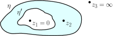
Figure 2: Illustration for Lemma 3.10. The blue region is $A_{\eta,\eta^{\prime}}$.

Lemma 3.10.

Let $G$ be the event that $\eta$ separates $z_{1}$ and $z_{3}$, and $\{z_{2}\in A_{\eta,\eta^{\prime}}\}$. Under the measure

$$1_{G}\mu_{h}(dz_{2})\,\mathbb{F}(dh)\,\mathrm{Count}_{\Gamma}(d\eta)\operatorname{CLE}_{\kappa}^{\mathbbm{C}}(d\Gamma),$$ (3.5)

the law of the decorated quantum surface $(h,\Gamma,z_{1},z_{2},z_{3})/{\sim_{\gamma}}$ is $\mathrm{QS}_{3}\otimes\operatorname{CLE}_{\kappa}$.

Proof.

Given $(h,\Gamma,z_{1},z_{2},z_{3})$ sampled from $\mu_{h}(dz_{2})\,\mathbb{F}(dh)\,\mathrm{Count}_{\Gamma}(d\eta)\operatorname{CLE}_{\kappa}^{\mathbbm{C}}(d\Gamma)$, for $i=1,2,3$, let $\eta_{i}$ be the outermost loop separating $z_{i}$ and $\{z_{1},z_{2},z_{3}\}\setminus\{z_{i}\}$. Then the event $G$ is the same as $\{\eta=\eta_{3}\}$. Since $\mathrm{Count}_{\Gamma}(d\eta)$ is simply the counting measure, the law of $(h,\Gamma,z_{1},z_{2},z_{3})$ under (3.5) is $\mu_{h}(dz_{2})\mathbb{F}(dh)\operatorname{CLE}_{\kappa}^{\mathbbm{C}}(d\Gamma)$. Now Lemma 3.10 follows from the definition of $\mathrm{QS}_{3}$. ∎

Let $p$ be sampled on $\eta$ from the probability measure proportional to the quantum length of $\eta$. By Proposition 3.9 and the definition of the uniform conformal welding, under the measure (3.5), conditioned on $(D_{\eta},h,\Gamma|_{D_{\eta}},z_{1},z_{2},p)/{\sim_{\gamma}}$, the conditional law of $(D_{\eta}^{c},h,z_{3},p)/{\sim_{\gamma}}$ is $\mathrm{QD}_{1,1}(\mathfrak{l})^{\#}$, where $\mathfrak{l}$ is the quantum length of $\eta$. From the proof of Lemma 3.10, on the event $G$, we have $\eta=\eta_{3}$ where $\eta_{3}$ is the outermost loop separating $z_{3}$ and $\{z_{1},z_{2}\}$. Therefore $D_{\eta}^{c}$ is the component of $\hat{\mathbbm{C}}\setminus\eta_{3}$ containing $z_{3}$. This yields the following proposition, which we immediately use to prove Theorem 3.7.

Proposition 3.11.

Suppose we are in the setting of Theorem 3.7. For $i=1,2,3$, let $D_{\eta_{i}}$ and $D^{c}_{\eta_{i}}$ be the two components of $\hat{\mathbbm{C}}\setminus\eta_{i}$ where $D_{\eta_{i}}$ contains $z_{i}$. Let $\mathfrak{l}_{i}$ be the quantum length of $\eta_{i}$. Let $p$ be a point sampled from the probability measure proportional to the quantum length measure of $\eta_{3}$. Then conditioned on $(D^{c}_{\eta_{3}},h,\eta_{1},\eta_{2},z_{1},z_{2},p)/{\sim_{\gamma}}$, the conditional law of $(D_{\eta_{3}},h,z_{3},p)/{\sim_{\gamma}}$ is $\mathrm{QD}_{1,1}(\mathfrak{l}_{3})^{\#}$.

Proof of Theorem 3.7.

Recall $P_{\eta_{1},\eta_{2},\eta_{3}}$ and $\widetilde{\mathrm{QP}}$ from Definition 3.6 . By symmetry, Proposition 3.11 still holds if $D_{\eta_{3}}$ is replaced by $D_{\eta_{1}}$ or $D_{\eta_{2}}$. Applying Proposition 3.11 to $D_{\eta_{1}}$, $D_{\eta_{2}}$, $D_{\eta_{3}}$, we see that conditioned on $(P_{\eta_{1},\eta_{2},\eta_{3}},h)/{\sim}$, the conditional law of $(D_{\eta_{i}},h,z_{i})/{\sim_{\gamma}}$ is $\mathrm{QD}_{1,0}(\mathfrak{l}_{i})^{\#}$ for $i=1,2,3$, and these three quantum disks are conditionally independent. Moreover the way they are welded to $P_{\eta_{1},\eta_{2},\eta_{3}}$ is according to the uniform conformal welding. Therefore, the law of $(\mathbbm{C},\phi,\eta_{1},\eta_{2},\eta_{3},z_{1},z_{2},z_{3})/{\sim_{\gamma}}$ is

$$\iiint_{\mathbbm{R}^{3}_{+}}\mathrm{Weld}\Big{(}\mathrm{QD}_{1,0}(\ell_{1})^{\#},\mathrm{QD}_{1,0}(\ell_{2})^{\#},\mathrm{QD}_{1,0}(\ell_{3})^{\#},\widetilde{\mathrm{QP}}(\ell_{1},\ell_{2},\ell_{3})\Big{)}\,d\ell_{1}\,d\ell_{2}\,d\ell_{3}.$$

Now Theorem 3.7 follows from $\mathrm{QD}_{1,0}(\ell)=|\mathrm{QD}_{1,0}(\ell)|\mathrm{QD}_{1,0}(\ell)^{\#}$ and the definition of $\mathrm{QP}$. ∎

We now prove Proposition 3.4 based on Theorem 3.7. We will use the following measures on decorated quantum surfaces. For $a>0$, let $(D,h,\Gamma,z)$ be an embedding of a sample from $\mathrm{QD}_{1,0}(a)\otimes\operatorname{CLE}_{\kappa}$. Let $\eta$ be the outermost loop of $\Gamma$ surrounding $z$. Let $\hat{\mathrm{QD}}_{1,0}(a)$ be the law of the decorated quantum surface $(D,h,\eta,z)/{\sim_{\gamma}}$. With these notations Proposition 3.4 is equivalent to

$$\hat{\mathrm{QD}}_{1,0}(a)=\int_{0}^{\infty}b\mathrm{Weld}(\mathrm{QA}(a,b),\mathrm{QD}_{1,0}(b))\,db.$$ (3.6)

Proof of Proposition 3.4 .

We retain the setting of Lemma 3.10 and use the notations there, with $(\eta^{\prime},\eta)$ there identified with $(\eta_{1},\eta_{3})$ as in Proposition 3.11. Let $\hat{\mathrm{QD}}_{1,0}^{\bullet}(a)=\mathcal{A}\hat{\mathrm{QD}}_{1,0}(a)$ where $\mathcal{A}$ is the quantum area of the annulus bounded by $\eta$ and $\partial D$. By Proposition 3.9, the law of $(h,\Gamma,\eta_{1},\eta_{3},z_{1},z_{3})/{\sim_{\gamma}}$ under the measure (3.5) is

$$C\int_{0}^{\infty}\ell_{3}\mathrm{Weld}(\hat{\mathrm{QD}}_{1,0}^{\bullet}(\ell_{3}),\mathrm{QD}_{1,0}(\ell_{3}))\,d\ell_{3}\quad\textrm{with $C$ the constant in Proposition~{}\ref{thm-loop3}.}$$ (3.7)

On the other hand, recall from Lemma 3.10 that the law of $(h,\Gamma,z_{1},z_{2},z_{3})$ under the measure (3.5) is $\mathrm{QS}_{3}\otimes\operatorname{CLE}_{\kappa}$. Let $\hat{\mathrm{QA}}^{\bullet}(\ell_{1},\ell_{3})$ be the law of a sample from

$$\int_{0}^{\infty}\ell_{2}\mathrm{Weld}\Big{(}\mathrm{QD}_{1,0}(\ell_{2}),\mathrm{QP}(\ell_{1},\ell_{2},\ell_{3})\Big{)}\,d\ell_{2}\quad\textrm{after forgetting the interior marked point and loop}.$$

Then by Theorem 3.7, the law of $(h,\Gamma,\eta_{1},\eta_{3},z_{1},z_{3})/{\sim_{\gamma}}$ is

$$\iint_{\mathbbm{R}^{2}_{+}}\ell_{1}\ell_{3}\mathrm{Weld}\Big{(}\mathrm{QD}_{1,0}(\ell_{1}),\hat{\mathrm{QA}}^{\bullet}(\ell_{1},\ell_{3}),\mathrm{QD}_{1,0}(\ell_{3})\Big{)}\,d\ell_{1}\,d\ell_{3}.$$

Therefore, for almost every $\ell_{3}\in(0,\infty)$ we have

$$C\mathrm{Weld}(\hat{\mathrm{QD}}_{1,0}^{\bullet}(\ell_{3}),\mathrm{QD}_{1,0}(\ell_{3}))=\int_{0}^{\infty}\ell_{1}\mathrm{Weld}\Big{(}\mathrm{QD}_{1,0}(\ell_{1}),\hat{\mathrm{QA}}^{\bullet}(\ell_{1},\ell_{3}),\mathrm{QD}_{1,0}(\ell_{3})\Big{)}\,d\ell_{1},$$

and hence

$$C\hat{\mathrm{QD}}_{1,0}^{\bullet}(\ell_{3})=\int_{0}^{\infty}\ell_{1}\mathrm{Weld}\Big{(}\mathrm{QD}_{1,0}(\ell_{1}),\hat{\mathrm{QA}}^{\bullet}(\ell_{1},\ell_{3})\Big{)}\,d\ell_{1}\quad\textrm{for a.e. }\ell_{3}>0.$$ (3.8)

Let $\hat{\mathrm{QA}}(\ell_{1},\ell_{3})=\mathcal{A}^{-1}\hat{\mathrm{QA}}^{\bullet}(\ell_{1},\ell_{3})$ where $\mathcal{A}$ is the quantum area of a sample from $\hat{\mathrm{QA}}^{\bullet}(\ell_{1},\ell_{3})$. Then

$$C\hat{\mathrm{QD}}_{1,0}(\ell_{3})=\int_{0}^{\infty}\mathrm{Weld}\Big{(}\mathrm{QD}_{1,0}(\ell_{1}),\hat{\mathrm{QA}}(\ell_{1},\ell_{3})\Big{)}\,d\ell_{1}\quad\textrm{for a.e. }\ell_{3}>0.$$ (3.9)

By scaling the quantum boundary length, we see that (3.9) holds for all $\ell_{3}>0$. Therefore, for a sample $(D,h,\eta,z)/{\sim_{\gamma}}$ from $\hat{\mathrm{QD}}_{1,0}(\ell_{3})$, the law of the annulus bounded by $\eta$ and $\partial D$ as a quantum surface is $C^{-1}\int_{0}^{\infty}|\mathrm{QD}_{1,0}(\ell_{1})|\hat{\mathrm{QA}}(\ell_{1},\ell_{3})\,d\ell_{1}$. By the definition of $\widetilde{\mathrm{QA}}$ and $\mathrm{QA}$ from Definition 3.2,

$$|\mathrm{QD}_{1,0}(\ell_{1})|\mathrm{QA}(\ell_{3},\ell_{1})=\widetilde{\mathrm{QA}}(\ell_{3},\ell_{1})=C^{-1}|\mathrm{QD}_{1,0}(\ell_{1})|\hat{\mathrm{QA}}(\ell_{1},\ell_{3})\quad\textrm{for all }\ell_{3}>0\textrm{ and a.e. }\ell_{1}>0.$$

Now (3.9) becomes $\hat{\mathrm{QD}}_{1,0}(\ell_{3})=\int_{0}^{\infty}\mathrm{Weld}\Big{(}\mathrm{QD}_{1,0}(\ell_{1}),\mathrm{QA}(\ell_{3},\ell_{1})\Big{)}\,d\ell_{1}$, which is equivalent to (3.6). ∎

Remark 3.12 (Symmetry of the quantum annulus).

Note that $\mathrm{QP}(\ell_{1},\ell_{2},\ell_{3})=\mathrm{QP}(\ell_{3},\ell_{2},\ell_{1})$ as measures on quantum surfaces with unlabeled boundary components. In the proof of Proposition 3.4, we have $\hat{\mathrm{QA}}^{\bullet}(\ell_{1},\ell_{3})=\int_{0}^{\infty}\ell_{2}\mathrm{Weld}\Big{(}\mathrm{QD}_{1,0}(\ell_{2}),\mathrm{QP}(\ell_{1},\ell_{2},\ell_{3})\Big{)}\,d\ell_{2}$ after forgetting the interior marked point and interface on the right hand side. Therefore $\hat{\mathrm{QA}}^{\bullet}(\ell_{1},\ell_{3})=\hat{\mathrm{QA}}^{\bullet}(\ell_{3},\ell_{1})$ hence $\mathrm{QA}(\ell_{1},\ell_{3})=\mathrm{QA}(\ell_{3},\ell_{1})$, as measures on quantum surfaces with unlabeled boundary components.

As a consequence of the proof of Proposition 3.4, we have the following lemma.

Lemma 3.13.

Suppose the law of $(D,h,\Gamma)/{\sim_{\gamma}}$ is $\mathcal{A}^{2}\mathrm{QD}(a)\times\operatorname{CLE}_{\kappa}$ where $\mathcal{A}$ is the total quantum area of the disk. Now independently sample $z,w\in D$ from the probability measure proportional to the quantum area measure. Let $\eta_{z}$ and $\eta_{w}$ be the outermost loops of $\Gamma$ surrounding $z$ and $w$, respectively. Let $F=\{\eta_{z}\neq\eta_{w}\}$. Then restricted to the event $F$, the law of $(D,h,\eta_{z},\eta_{w},z,w)/{\sim_{\gamma}}$ is $C\iint_{\mathbbm{R}_{+}^{2}}bc\mathrm{Weld}\mathopen{}\mathclose{{}\left(\mathrm{QD}_{1,0}(b),\mathrm{QD}_{1,0}(c),\mathrm{QP}(a,b,c)}\right)\,db\,dc$ for some $C\in(0,\infty)$.

Proof.

From the proof of Proposition 3.4, we see that the law of $(D,h,\eta_{z},z)/{\sim_{\gamma}}$ is $\hat{\mathrm{QD}}_{1,0}^{\bullet}(a)$. By (3.8) and the fact that $\hat{\mathrm{QA}}^{\bullet}(\ell_{1},\ell_{3})$ is obtained from $\int_{0}^{\infty}\ell_{2}\mathrm{Weld}\Big{(}\mathrm{QD}_{1,0}(\ell_{2}),\mathrm{QP}(\ell_{1},\ell_{2},\ell_{3})\Big{)}\,d\ell_{2}$ after forgetting the interior marked point and interface, we get the desired welding result. ∎

We conclude this section with the following lemma needed in Section 4.

Lemma 3.14.

For $a>0$, sample $(D,h,\Gamma,z)/{\sim_{\gamma}}$ from $\mathrm{QD}_{1,0}(a)\otimes\operatorname{CLE}_{\kappa}$ and sample $\hat{\eta}$ from the counting measure on the outermost loops of $\Gamma$ except the loop $\eta$ surrounding $z$. Then the law of $(D,h,\eta,\hat{\eta},z)/{\sim_{\gamma}}$ is $C\iint_{\mathbbm{R}^{2}_{+}}bc\mathrm{Weld}\mathopen{}\mathclose{{}\left(\mathrm{QD}_{1,0}(b),\mathrm{QD}(c),\mathrm{QP}(a,b,c)}\right)\,db\,dc$ for some constant $C\in(0,\infty)$.

Proof.

Let $D_{\hat{\eta}}$ be the region encircled by $\hat{\eta}$. Now reweight the law of $(D,h,\eta,\hat{\eta},z)/{\sim_{\gamma}}$ by $\mu_{h}(D_{\hat{\eta}})$ and sample $w\in D_{\hat{\eta}}$ according to the probability measure proportional to the area measure $\mu_{h}|_{D_{\hat{\eta}}}$. Then the law of $(D,h,\eta,\hat{\eta},z,w)/{\sim_{\gamma}}$ under the reweighted measure is the same as the law of $(D,h,\eta_{z},\eta_{w},z,w)/{\sim_{\gamma}}$ in Lemma 3.13, which equals $C\iint_{\mathbbm{R}_{+}^{2}}bc\mathrm{Weld}\mathopen{}\mathclose{{}\left(\mathrm{QD}_{1,0}(b),\mathrm{QD}_{1,0}(c),\mathrm{QP}(a,b,c)}\right)\,db\,dc$. Unweighting by $\mu_{h}(D_{\hat{\eta}})$ and forgetting $w$, we obtain the desired law of $(D,h,\eta,\hat{\eta},z)/{\sim_{\gamma}}$. ∎

4 Area and length distributions of $\mathrm{QA}$ and $\mathrm{QP}$

In this section we prove the analog of the FZZ formula (Theorem 2.16) for the quantum annulus $\mathrm{QA}(a,b)$ from Definition 3.2 and for the quantum pair of pants $\mathrm{QP}(a,b,c)$ from Definition 3.6. We assume $\kappa\in(\frac{8}{3},4)$ and $\gamma=\sqrt{\kappa}$ throughout this section.

Theorem 4.1.

For $a>0,b>0$, let $A$ be the quantum area of a sample from $\mathrm{QA}(a,b)$. Then

$$\mathrm{QA}(a,b)[e^{-\mu A}]=\frac{\cos(\pi(\frac{4}{\gamma^{2}}-1))}{\pi}\cdot\frac{e^{-(a+b)\sqrt{\mu/\sin(\pi\gamma^{2}/4)}}}{\sqrt{ab}(a+b)}\quad\textrm{for }\mu\geq 0.$$

Theorem 4.2.

For $\ell_{1},\ell_{2},\ell_{3}>0$. let $A$ be the total quantum area of a sample from $\mathrm{QP}(\ell_{1},\ell_{2},\ell_{3})$. Then there is a constant $C\in(0,\infty)$ only depending on $\gamma$ such that

$$\mathrm{QP}(\ell_{1},\ell_{2},\ell_{3})[e^{-\mu A}]=C\mu^{\frac{1}{4}-\frac{2}{\gamma^{2}}}\frac{1}{\sqrt{\ell_{1}\ell_{2}\ell_{3}}}e^{-(\ell_{1}+\ell_{2}+\ell_{3})\sqrt{\mu/\sin(\pi\gamma^{2}/4)}}\quad\textrm{for }\mu>0.$$

Setting $\mu=0$ in Theorem 4.1, we see that $\mathrm{QA}(a,b)$ is a finite measure. Sending $\mu$ to $0$ in Theorem 4.2, we see that $\mathrm{QP}(\ell_{1},\ell_{2},\ell_{3})$ is infinite. However, since $\mathrm{QP}(\ell_{1},\ell_{2},\ell_{3})[A<x]<\infty$ for $x>0$, it is still $\sigma$-finite.

In the rest of this section, we first compute $|\mathrm{QA}(a,b)|$ up to a multiplicative constant in Sections 4.1 and 4.2. Then we prove Theorem 4.1 and 4.2 in Sections 4.3 and 4.4, respectively. Although not needed, we evaluate the constant $C$ in Theorem 4.2 at the end of Section 4.4.

4.1 Length distribution for the quantum annulus: the first reduction

In this and the next subsection, we prove Proposition 4.3, which is the $\mu=0$ case of Theorem 4.1.

Proposition 4.3.

For $a>0,b>0$, the total mass $\mathopen{}\mathclose{{}\left|\mathrm{QA}(a,b)}\right|$ of $\mathrm{QA}(a,b)$ is given by

$$\mathopen{}\mathclose{{}\left|\mathrm{QA}(a,b)}\right|=\frac{\cos(\pi(\frac{4}{\gamma^{2}}-1))}{\pi\sqrt{ab}(a+b)}.$$

In this subsection we reduce Proposition 4.3 to the setting of Proposition 2.21 in order to use the Levy process defined there. Recall that setting where $(D,h,\Gamma)$ is an embedding from a sample of $\mathrm{QD}(a)^{\#}\otimes\operatorname{CLE}_{\kappa}$ for some $a>0$. Sample a loop $\eta$ from the counting measure on $\Gamma$, and let $\mathbb{M}_{a}$ be the law of the decorated quantum surface $(D,h,\Gamma,\eta)$. In other words, consider $((D,h,\Gamma)/{\sim_{\gamma}},\mathbf{n})$ sampled from the product measure $(\mathrm{QD}(a)^{\#}\otimes\operatorname{CLE}_{\kappa})\times\mathrm{Count}_{\mathbb{N}}$ where $\mathrm{Count}_{\mathbb{N}}$ is the counting measure on $\mathbb{N}$. Let $\eta\in\Gamma$ be the outermost loop with the ${\mathbf{n}}$th largest quantum length. Then $\mathbb{M}_{a}$ is the law of $(D,h,\Gamma,\eta)/{\sim_{\gamma}}$. The following proposition is the analog of Proposition 3.4 for $\mathbb{M}_{a}$.

Proposition 4.4.

Under $\mathbb{M}_{a}$, the law of $(D,h,\eta)/{\sim_{\gamma}}$ is

$$\frac{1}{|\mathrm{QD}(a)|}\int_{0}^{\infty}b\mathrm{Weld}(\mathrm{QA}(a,b),\mathrm{QD}(b))\,db.$$

Proof.

Let $\mathbb{F}$ be a measure on $H^{-1}(\mathbbm{D})$ such that the law of $(\mathbbm{D},h)/{\sim_{\gamma}}$ is $\mathrm{QD}(a)$ if $h$ is a sample from $\mathbb{F}$. We write $\operatorname{CLE}_{\kappa}(d\Gamma)$ as the probability measure for $\operatorname{CLE}_{\kappa}$ on $\mathbbm{D}$. Write $\mathrm{Count}_{\Gamma^{o}}(d\eta)$ as the counting measure on the set of outermost loops in $\Gamma$. By the definition of $\mathbb{M}_{a}$, under the measure $\mathrm{Count}_{\Gamma^{o}}(d\eta)\,\mathbb{F}(dh)\operatorname{CLE}_{\kappa}(d\Gamma)$, the law of $(h,\Gamma,\eta)/{\sim_{\gamma}}$ is $|\mathrm{QD}(a)|\cdot\mathbb{M}_{a}$.

On the other hand, under the measure $\mu_{h}|_{D_{\eta}}(dz)\mathrm{Count}_{\Gamma^{o}}(d\eta)\,\mathbb{F}(dh)\operatorname{CLE}_{\kappa}(d\Gamma)$, the law of $(\mathbbm{D},h,\Gamma,z)/{\sim_{\gamma}}$ is $\mathrm{QD}_{1,0}(a)\otimes\operatorname{CLE}_{\kappa}$ and $\eta$ is the outermost loop around $z$. By Proposition 3.4 the law of $(\mathbbm{D},h,\eta,z)/{\sim_{\gamma}}$ is $\int_{0}^{\infty}b\mathrm{Weld}(\mathrm{QA}(a,b),\mathrm{QD}_{1,0}(b))\,db$. Unweighting by $\mu_{h}(D_{\eta})$ and forgetting $z$, the law of $(D,h,\eta)/{\sim_{\gamma}}$ under $\mathrm{Count}_{\Gamma^{o}}(d\eta)\,\mathbb{F}(dh)\operatorname{CLE}_{\kappa}(d\Gamma)$ is $\int_{0}^{\infty}b\mathrm{Weld}(\mathrm{QA}(a,b),\mathrm{QD}(b))\,db$. ∎

Proposition 4.3 immediately follows from its counterpart Proposition 4.5 under $\mathbb{M}_{a}$.

Proposition 4.5.

The law of the quantum length of $\eta$ under $\mathbb{M}_{a}$ is

$$\frac{C1_{b>0}b|\mathrm{QD}(b)|db}{\sqrt{ab}(a+b)|\mathrm{QD}(a)|}\quad\textrm{where}\quad C=\frac{\cos(\pi(\frac{4}{\gamma^{2}}-1))}{\pi}.$$ (4.1)

Proof of Proposition 4.3 assuming Proposition 4.5.

By Proposition 4.4, the law of $\ell_{h}(\eta)$ under $\mathbb{M}_{a}$ is $1_{b>0}\frac{1}{|\mathrm{QD}(a)|}b|\mathrm{QA}(a,b)||\mathrm{QD}(b)|\,db$. Comparing this to Proposition 4.5 yields $|\mathrm{QA}(a,b)|=\frac{C}{\sqrt{ab}(a+b)}$. ∎

4.2 Length distribution for the quantum annulus: proof of Proposition 4.5

We now reduce Proposition 4.5 to a problem on the Levy process in Proposition 2.21. Let

$${\beta}=\frac{4}{\kappa}+\frac{1}{2}=\frac{4}{\gamma^{2}}+\frac{1}{2}\in(\frac{3}{2},2).$$ (4.2)

Let $\mathbbm{P}^{\beta}$ be the probability measure on càdlàg processes on $[0,\infty)$ describing the law of a ${\beta}$-stable Lévy process with Lévy measure $1_{x>0}x^{-\beta-1}\,dx$. Let $(\zeta_{t})_{t\geq 0}$ be a sample from $\mathbbm{P}^{\beta}$. Let $J:=\{(x,t):t\geq 0\textrm{ and }\zeta_{t}-\zeta_{t^{-}}=x>0\}$ be the set of jumps of $\zeta$. Given $J$, let $({\mathbf{b}},{\mathbf{t}})\in J$ be sampled from the counting measure on $J$. Let $M^{\beta}$ be the law of $(\zeta,{\mathbf{b}},{\mathbf{t}})$. Namely, $M^{\beta}$ is the infinite measure such that for non-negative measurable functions $f,g$ we have

$$M^{\beta}[f(\zeta)g({\mathbf{b}},{\mathbf{t}})]=\int\big{(}f(\zeta)\sum_{(x,t)\in J}g(x,t)\big{)}d\mathbbm{P}^{\beta}.$$

For each $a>0$, let $\tau_{-a}=\inf\{t:\zeta_{t}=-a\}$ and $J_{a}=\{(x,t)\in J:t\leq\tau_{-a}\}$. Let $M^{\beta}_{a}$ be the restriction of the measure $M^{\beta}$ to the event $\{{\mathbf{t}}\leq\tau_{-a}\}$. Let $\widetilde{M}^{\beta}_{a}=\frac{\tau_{-a}^{-1}}{\mathbbm{E}^{\beta}[\tau_{-a}^{-1}]}M^{\beta}_{a}$, where $\mathbbm{E}^{\beta}$ is the expectation with respect to $\mathbbm{P}^{\beta}$. Then by Proposition 2.21 we have the following.

Lemma 4.6.

Suppose $(D,h,\Gamma,\eta)$ and $\mathbb{M}_{a}$ are as in Proposition 4.4. Let $\ell_{1}>\ell_{2}>\dots$ be the quantum lengths of the outermost loops in $\Gamma$ and $\ell_{h}(\eta)$ be the quantum length of the distinguished loop $\eta$. Then the joint law of $\{\ell_{i}:i\geq 1\}$ and $\ell_{h}(\eta)$ under $\mathbb{M}_{a}$ equals the joint law of $\{x:(x,t)\in J\}$ and ${\mathbf{b}}$ under the measure $\widetilde{M}^{\beta}_{a}$ defined right above.

Proof.

Under the measure $\widetilde{M}_{a}^{\beta}$, the jump $({\mathbf{b}},{\mathbf{t}})$ is chosen from the counting measure of $J_{a}$. Since $\eta$ is chosen from the counting measure of outermost loops, Proposition 2.21 yields Lemma 4.6. ∎

Given Lemma 4.6, Proposition 4.5 immediately follows from the proposition below.

Proposition 4.7.

The law of ${\mathbf{b}}$ under $\widetilde{M}^{\beta}_{a}$ is

$$\frac{C1_{b>0}}{(a+b)}\mathopen{}\mathclose{{}\left(\frac{a}{b}}\right)^{{\beta}+1}db\quad\textrm{where}\quad C=\frac{\cos(\pi(\frac{4}{\gamma^{2}}-1))}{\pi}.$$ (4.3)

Proof of Proposition 4.5 given Proposition 4.7.

By Remark 2.15 we have $|\mathrm{QD}(b)|/|\mathrm{QD}(a)|=(a/b)^{{\beta}+\frac{3}{2}}$. By Lemma 4.6 and Proposition 4.7, the $\mathbb{M}_{a}$-law of the quantum length of $\eta$ is

$$\frac{C1_{b>0}}{(a+b)}\mathopen{}\mathclose{{}\left(\frac{a}{b}}\right)^{{\beta}+1}db=\frac{C1_{b>0}b|\mathrm{QD}(b)|db}{\sqrt{ab}(a+b)|\mathrm{QD}(a)|}.\qed$$

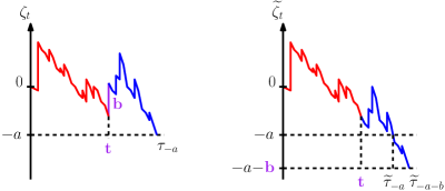
Figure 3: Illustration for Lemmas 4.8 and 4.9. The measure $M^{\beta}$ is $\mathbbm{P}^{\beta}$ with a uniformly chosen jump $(\mathbf{b},\mathbf{t})$ shown in purple. Concatenating the two pieces of $(\zeta_{t})$ (shown in red and blue)

before and after ${\mathbf{t}}$ gives a sample $(\widetilde{\zeta}_{t})_{t\geq 0}$ of $\mathbbm{P}^{\beta}$. The event $\{{\mathbf{t}}<\tau_{-a}\}$ for $\zeta$ becomes $\{{\mathbf{t}}<\widetilde{\tau}_{-a}\}$ for $\widetilde{\zeta}$.

To prove Proposition 4.7, we first use Palm’s Theorem for Poisson point processes to give an alternative description of the measure $M^{\beta}$. See Figure 3 for an illustration.

Lemma 4.8.

Let $\widetilde{\zeta}_{t}=\zeta_{t}-1_{t\geq{\mathbf{t}}}{\mathbf{b}}$. Then the $M^{\beta}$-law of $({\mathbf{b}},{\mathbf{t}})$ is $1_{b>0,t>0}b^{-\beta-1}\,db\,dt$, and conditioning on $({\mathbf{b}},{\mathbf{t}})$, the conditional law of $\widetilde{\zeta}_{t}$ under $M^{\beta}$ is $\mathbbm{P}^{\beta}$. Equivalently, the joint law of $({\mathbf{b}},{\mathbf{t}})$ and $(\widetilde{\zeta}_{t})_{t\geq 0}$ under $M^{\beta}$ is the product measure $(1_{b>0,t>0}b^{-\beta-1}\,db\,dt)\times\mathbbm{P}^{\beta}$.

Proof.

By the definition of Levy measure, the jump set $J$ of $\zeta$ is a Poisson point process on $(0,\infty)^{2}$ with intensity measure $1_{x>0,t>0}x^{-\beta-1}\,dx\,dt$. Since $({\mathbf{b}},{\mathbf{t}})$ is chosen from the counting measure on $J$, by Palm’s theorem (see e.g. [Kal17, Page 5]), the $M^{\beta}$-law of $({\mathbf{b}},{\mathbf{t}})$ is the same as the intensity measure of $J$, which is $1_{b>0,t>0}b^{-\beta-1}\,db\,dt$. Moreover, conditioning on $({\mathbf{b}},{\mathbf{t}})$, the conditional law of $J\setminus\{({\mathbf{b}},{\mathbf{t}})\}$ is given by the original Poisson point process, which is the $\mathbbm{P}^{\beta}$-law of $J$. Note that $(\widetilde{\zeta}_{t})_{0\leq t<{\mathbf{t}}}=(\zeta_{t})_{0\leq t<{\mathbf{t}}}$ is measurable with respect to the jump set $\{(x,t)\in J:t<{\mathbf{t}}\}$. Therefore, the conditional law of $(\widetilde{\zeta}_{t})_{0\leq t<{\mathbf{t}}}$ conditioning on $({\mathbf{b}},{\mathbf{t}})$ is the $\mathbbm{P}^{\beta}$-law of $(\zeta_{t})_{0\leq t<{\mathbf{t}}}$. Similarly, conditioning on $({\mathbf{b}},{\mathbf{t}})$ and $(\widetilde{\zeta}_{t})_{0\leq t<{\mathbf{t}}}$, the conditional law of $(\widetilde{\zeta}_{t+{\mathbf{t}}}-\widetilde{\zeta}_{{\mathbf{t}}})_{t\geq 0}$ under $M^{\beta}$ is $\mathbbm{P}^{\beta}$. Concatenating $(\widetilde{\zeta}_{t})_{0\leq t<{\mathbf{t}}}$ and $(\widetilde{\zeta}_{t+{\mathbf{t}}}-\widetilde{\zeta}_{{\mathbf{t}}})_{t\geq 0}$ we see that the conditional law of $\widetilde{\zeta}_{t}$ under $M^{\beta}$ is $\mathbbm{P}^{\beta}$. ∎

Now Proposition 4.7 is an immediate consequence of the following two lemmas.

Lemma 4.9.

Let $(\zeta_{t})_{t\geq 0}$ be sampled from $\mathbbm{P}^{\beta}$ and $\tau_{-a}=\inf\{t:\zeta_{t}=-a\}$ for each $a>0$. Let $\mathbbm{E}^{\beta}$ be the expectation for $\mathbbm{P}^{\beta}$. Then the law of ${\mathbf{b}}$ under $\widetilde{M}^{\beta}_{a}$ in Proposition 4.7 is

$$\frac{\mathbbm{E}^{\beta}\mathopen{}\mathclose{{}\left[{\tau_{-a}}/{\tau_{-a-b}}}\right]}{\mathbbm{E}^{\beta}[\tau^{-1}_{-a}]}b^{-{\beta}-1}1_{b>0}db.$$

Proof.

We start from $(\zeta_{t})_{t\geq 0}$ and $({\mathbf{b}},{\mathbf{t}})$ under $M^{\beta}$. Let $\widetilde{\zeta}_{t}=\zeta_{t}-1_{t\geq{\mathbf{t}}}{\mathbf{b}}$ as in Lemma 4.8. Let $\widetilde{\tau}_{-\ell}=\inf\{t:\widetilde{\zeta}_{t}=-\ell\}$ for each $\ell>0$. Both the events $\{{\mathbf{t}}<\tau_{-a}\}$ and $\{{\mathbf{t}}<\widetilde{\tau}_{-a}\}$ are the same as $\inf\{\zeta_{t}:t\in(0,{\mathbf{t}})\}>-a$, hence are equal. Moreover, on $\{{\mathbf{t}}<\tau_{-a}\}$ we have $\tau_{-a}=\widetilde{\tau}_{-a-{\mathbf{b}}}$. Now the measure $\widetilde{M}^{\beta}_{a}$ can be described as

$$\frac{\tau^{-1}_{-a}}{\mathbbm{E}^{\beta}[\tau^{-1}_{-a}]}M^{\beta}_{a}=\frac{\tau^{-1}_{-a}1_{{\mathbf{t}}<\tau_{-a}}}{\mathbbm{E}^{\beta}[\tau^{-1}_{-a}]}M^{\beta}=\frac{\widetilde{\tau}^{-1}_{-a-{\mathbf{b}}}1_{{\mathbf{t}}<\widetilde{\tau}_{-a}}}{\mathbbm{E}^{\beta}[\tau^{-1}_{-a}]}M^{\beta}.$$ (4.4)

Integrating out ${\mathbf{t}}$ and $(\widetilde{\zeta}_{t})_{t\geq 0}$ on the right side of (4.4) and using the joint law of $({\mathbf{b}},{\mathbf{t}})$ and $(\widetilde{\zeta}_{t})_{t\geq 0}$ from Lemma 4.8, we see that the $\widetilde{M}^{\beta}_{a}$-law of ${\mathbf{b}}$ is $\frac{\mathbbm{E}^{\beta}\mathopen{}\mathclose{{}\left[{\tau_{-a}}/{\tau_{-a-b}}}\right]}{\mathbbm{E}^{\beta}[\tau^{-1}_{-a}]}b^{-{\beta}-1}1_{b>0}db$ as desired. ∎

Lemma 4.10.

We have $\mathbbm{E}^{\beta}\mathopen{}\mathclose{{}\left[{\tau_{-a}}/{\tau_{-a-b}}}\right]=\frac{a}{a+b}$ for each $a,b>0$. Moreover, $\mathbbm{E}[\tau_{-1}^{-1}]=\frac{\pi}{\sin(-\pi\beta)}$.

Proof.

The process $(\tau_{-s})_{s\geq 0}$ is a stable subordinator of index $1/\beta$. Since $(\tau_{-a},\tau_{-2a})$ has the distribution as $(\tau_{-2a}-\tau_{-a},\tau_{-2a})$, we have $\mathbbm{E}^{\beta}\mathopen{}\mathclose{{}\left[{\tau_{-a}}/{\tau_{-2a}}}\right]=\frac{1}{2}$. Similary, we have $\mathbbm{E}^{\beta}\mathopen{}\mathclose{{}\left[{\tau_{-a}}/{\tau_{-b}}}\right]=\frac{a}{a+b}$ if $\frac{a}{b}$ is rational. By continuity we can extend this to all $a,b>0$. For the second equality, let $(Y_{t})_{t\geq 0}$ be the Levy process with Levy measure $\Pi(dx)=\Gamma(-\beta)^{-1}1_{x>0}x^{-\beta-1}dx$ so that $\mathbbm{E}[e^{-\lambda Y_{t}}]=e^{t\lambda^{\beta}}$. Let $\sigma_{-s}=\inf\{t\geq 0:Y_{t}=-s\}$ for $s>0$. Then $\mathbbm{E}[e^{-\lambda\sigma_{-s}}]=e^{s\lambda^{1/\beta}}$ and $\mathbbm{E}[\sigma_{-1}^{-1}]=\int_{0}^{\infty}\mathbbm{E}[e^{-\lambda\sigma_{-1}}]d\lambda=\Gamma(1+\beta)$. By scaling, we have $\mathbbm{E}[\tau_{-1}^{-1}]=\Gamma(-\beta)\mathbbm{E}[\sigma^{-1}_{-1}]=\Gamma(-\beta)\Gamma(1+\beta)=\frac{\pi}{\sin(-\pi\beta)}$. ∎

Proof of Proposition 4.7.

With respect to $\mathbbm{P}^{\beta}$, we have $\tau_{-a}\stackrel{{\scriptstyle d}}{{=}}a^{\beta}\tau_{-1}$ by the scaling property of ${\beta}$-stable Lévy processes. Therefore $\mathbbm{E}^{\beta}[\tau^{-1}_{-a}]=\mathbbm{E}^{\beta}[\tau^{-1}_{-1}]a^{-{\beta}}$. Combined with Lemmas 4.9 and 4.10 we get (4.3) with $C=1/\mathbbm{E}^{{\beta}}[\tau^{-1}_{-1}]=(\pi)^{-1}\sin(-\pi\beta)=(\pi)^{-1}\cos(\pi(\frac{4}{\gamma^{2}}-1))$. ∎

We conclude this section with two by-products of our proof of Proposition 4.5. They will be needed in Sections 4.3 and 4.4. The first one is a description of the quantum lengths of all the outermost loops in $\Gamma$ except $\eta$ and the laws of the quantum surfaces encircled by these loops.

Proposition 4.11.

For $a>0$, let $(D,h,\Gamma,z)/{\sim_{\gamma}}$ be a sample from $\mathrm{QD}_{1,0}(a)\otimes\operatorname{CLE}_{\kappa}$. Let $(\ell_{i})_{i\geq 1}$ be the quantum lengths of the outermost loops in $\Gamma$ and $\ell_{h}(\eta)$ the quantum length of the loop $\eta$ surrounding $z$. Then conditioned on $\ell_{h}(\eta)$, the conditional law of $\{\ell_{i}:\ell_{i}\neq\ell_{h}(\eta),i\geq 1\}$ equals the $\mathbbm{P}^{\beta}$-law of $\{x:(x,t)\in J_{a+\ell_{h}(\eta)}\textrm{ for some }t\}$. Moreover, conditioned on $(\ell_{i})_{i\geq 1}$, the quantum surfaces encircled by these outermost loops apart from $\eta$ are independent quantum disks with boundary lengths $\{\ell_{i}:\ell_{i}\neq\ell_{h}(\eta),i\geq 1\}$.

Proof.

By Propositions 3.4 and 4.4, the conditional law of $\{\ell_{i}:i\geq 1,\ell_{i}\neq\ell_{h}(\eta)\}$ given $\ell_{h}(\eta)=b$ under $\mathbb{M}_{a}$ in Lemma 4.6 is the same as under $\mathrm{QD}_{1,0}(a)\otimes\operatorname{CLE}_{\kappa}$ in the current proposition. By Lemma 4.6, it is the same as the conditional law of $\{x:(x,t)\in J,x\neq b\}$ given ${\mathbf{b}}=b$ under the measure $\widetilde{M}^{\beta}_{a}$. By Lemma 4.8, it equals the $\mathbbm{P}^{\beta}$-law of $\{x:(x,t)\in J_{a+b}\textrm{ for some }t\}$. The second statement on the law of quantum surfaces encircled by these outermost loops follows from Proposition 2.22. ∎

The second fact is a simple corollary of Proposition 4.11 and Lemma 4.8.

Lemma 4.12.

For $a>0$, let $(D,h,\Gamma,z)/{\sim_{\gamma}}$ be a sample from $\mathrm{QD}_{1,0}(a)\otimes\operatorname{CLE}_{\kappa}$ and $\eta$ be the outermost loop surrouding $z$. Let $\hat{\eta}$ be chosen from the counting measure on the outermost loops of $\Gamma$ except $\eta$. Let $(\ell_{i})_{i\geq 1}$ be the lengths of the outermost loops of $\Gamma$ except $\eta$ and $\hat{\eta}$, ranked in decreasing order. Then for $b,c>0$, the disintegration of the law of $\{\ell_{i}:i\geq 1\}$ over $\{\ell_{h}(\eta)=b,\ell_{h}(\hat{\eta})=c\}$ is the law of $\{x:(x,t)\in J_{a+b+c}\textrm{ for some }t\}$ under

$$b|\mathrm{QA}(a,b)||\mathrm{QD}_{1,0}(b)|c^{-\beta-1}\tau_{-a-b}\mathbbm{P}^{\beta}(d\zeta).$$

Proof.

By Propositions 3.4 and 4.11, the disintegration of the law of $\{\ell_{i}:\ell_{i}\neq\ell_{h}(\eta),i\geq 1\}$ over $\{\ell_{h}(\eta)=b\}$ is the law of $\{x:(x,t)\in J_{a+b}\textrm{ for some }t\}$ under

$$b|\mathrm{QA}(a,b)||\mathrm{QD}_{1,0}(b)|\mathbbm{P}^{\beta}(d\zeta).$$

Since we further remove the loop $\hat{\eta}$ chosen from counting measure, by Lemma 4.8, we get the additional factor $c^{-\beta-1}\tau_{-a-b}$ and the change from $J_{a+b}$ to $J_{a+b+c}$ for the jump set. ∎

4.3 Area distribution for the quantum annulus

In this section we prove Theorem 4.1 using the conformal welding result Proposition 3.4 for the quantum annulus and the FZZ formula Theorem 2.16. Since $\mathrm{QA}(a,b)=|\mathrm{QA}(a,b)|\mathrm{QA}(a,b)^{\#}$, it remains to compute $\mathrm{QA}^{\#}(a,b)[e^{-\mu A}]$. Recall $\mathbbm{P}^{\beta}$ from Proposition 2.21 with $\beta=\frac{4}{\gamma^{2}}+\frac{1}{2}$. Let $(\zeta_{t})_{t\geq 0}$ be a stable Lévy process with index ${\beta}$ sampled from $\mathbbm{P}^{\beta}$. For $L>0$, let $\tau_{-L}=\inf\{t\>:\>\zeta_{t}\leq-L\}$. Our starting point is the following lemma.

Lemma 4.13.

For $a,b>0$, let $(x_{i})_{i\geq 1}$ be the collection of sizes of the jumps of $\zeta$ on $[0,\tau_{-a-b}]$ sorted in decreasing order. Let $(A_{i})_{i\geq 1}$ be independent copies of the quantum area of a sample from $\mathrm{QD}(1)^{\#}$ which are also independent of $(x_{i})_{i\geq 1}$. Then the quantum area of a sample from $\mathrm{QA}(a,b)^{\#}$ has the law of $\sum x_{i}^{2}A_{i}$.

Proof.

This follows from Proposition 4.11 and the scaling relation of quantum area and length. ∎

To compute $\mathbbm{E}[e^{-\mu\sum x_{i}^{2}A_{i}}]$ in Lemma 4.13, we need the following fact about the processes $\zeta$.

Lemma 4.14.

Fix $L>0$. Let $(x_{i})_{i\geq 1}$ be the collection of sizes of the jumps of $\zeta$ on $[0,\tau_{-L}]$ sorted in decreasing order. Let $(A_{i})_{i\geq 1}$ be independent and identically distributed positive random variables independent of $(x_{i})_{i\geq 1}$. Then for a constant $\lambda\in(0,\infty]$ not depending on $L$ we have

$$\mathbbm{E}[e^{-\mu\sum x_{i}^{2}A_{i}}]=e^{-L\lambda\sqrt{\mu}}\quad\text{for }\mu\geq 0,$$ (4.5)

where we use the convention $e^{-\infty}:=0$.

Proof.

Let $f(L)=\mathbbm{E}[e^{-\sum x_{i}^{2}A_{i}}]\in[0,1)$. By the Markov property of the stable Lévy process $\zeta$ and the independence of the $(A_{i})_{i\geq 1}$, we have $f(a+b)=f(a)f(b)$ for all $a,b>0$. Therefore there exists $\lambda\in(0,\infty]$ such that $f(L)=e^{-\lambda L}$ for all $L>0$. For $\mu>0$, by the scaling property of stable Lévy processes, the set of jumps $(x_{i})_{i\geq 1}$ of $\zeta$ on $[0,\tau_{-L}]$ agrees in law with $(\mu^{-1/2}y_{i})_{i\geq 1}$, where $(y_{i})_{i\geq 1}$ are the jumps of $\zeta$ on $[0,\tau_{-\mu^{1/2}L}]$. Therefore $\mathbbm{E}[e^{-\mu\sum x_{i}^{2}A_{i}}]=f(\mu^{1/2}L)=e^{-L\sqrt{\mu}\lambda}$ as desired. ∎

Proof of Theorem 4.1.

By Proposition 4.3, Lemmas 4.13 and 4.14, there exists $\lambda\in(0,\infty]$ such that

$$\mathrm{QA}(a,b)[e^{\mu A}]=\frac{\cos(\pi(\frac{4}{\gamma^{2}}-1))}{\pi}\cdot\frac{e^{-(a+b)\lambda\sqrt{\mu}}}{\sqrt{ab}(a+b)}.$$ (4.6)

It remains to prove that $\lambda=\sqrt{\frac{1}{\sin(\pi\gamma^{2}/4)}}$. By the conformal welding result Proposition 3.4 and the additivity of quantum areas, we have

$$\mathrm{QD}_{1,0}(a)[e^{-\mu A_{1}}]=\int_{0}^{\infty}b\mathrm{QA}(a,b)[e^{-\mu A_{2}}]\mathrm{QD}_{1,0}(b)[e^{-\mu A_{3}}]\,db$$

where $A_{1},A_{2},A_{3}$ represent the quantum areas of the respective quantum surfaces.

Set $\nu=\frac{2}{\gamma}(Q-\gamma)\in(0,\frac{1}{2})$. By (4.6) and the FZZ formula Theorem 2.16, we have

$$a^{-1}K_{\nu}(a\sqrt{\frac{\mu}{\sin(\pi\gamma^{2}/4)}})=\int_{0}^{\infty}b\frac{\cos(\pi\nu)}{\pi}\cdot\frac{e^{-(a+b)\lambda\sqrt{\mu}}}{\sqrt{ab}(a+b)}b^{-1}K_{\nu}(b\sqrt{\frac{\mu}{\sin(\pi\gamma^{2}/4)}})\,db.$$

Setting $a=1$, $x=\sqrt{\mu/\sin(\pi\gamma^{2}/4)}$ and $\lambda^{\prime}=\lambda\sqrt{\sin(\pi\gamma^{2}/4)}$, and integrating over $x$, we get

$$\int_{0}^{\infty}K_{\nu}(x)\,dx=\frac{\cos(\pi\nu)}{\pi}\iint_{0}^{\infty}\frac{1}{\sqrt{b}(b+1)}e^{-x(b+1)\lambda^{\prime}}K_{\nu}(xb)\,db\,dx.$$ (4.7)

Since $K_{\nu}(xb)>0$ for $xb>0$, the right hand side of (4.7) is decreasing in $\lambda^{\prime}$. Therefore there is a unique $\lambda^{\prime}$ for which (4.7) holds. By [DLMF, (10.43.18)], the left hand side of (4.7) equals $\frac{\pi}{2\cos(\frac{1}{2}\pi\nu)}$. By (2.8), the right hand side of (4.7) equals $\frac{\pi}{2\cos(\frac{1}{2}\pi\nu)}$ if $\lambda^{\prime}=1$. Therefore $\lambda^{\prime}=1$ as desired. ∎

As a corollary of the proof of Theorem 4.1, we have the following fact on the Levy process $\zeta$.

Proposition 4.15.

The constant $\lambda$ in Lemma 4.14 equals $\sqrt{\frac{1}{\sin(\pi\gamma^{2}/4)}}$ if $A_{i}$ there has the law of the quantum area of a sample from $\mathrm{QD}(1)^{\#}$.

4.4 Area and length distributions for the quantum pair of pants

In this section we prove Theorem 4.2. Our proof is based on the Levy process as in Section 4.2 and the conformal welding result Lemma 3.14. Recall $\mathbbm{P}^{\beta}$ from Proposition 2.21 with $\beta=\frac{4}{\gamma^{2}}+\frac{1}{2}$. Let $(\zeta_{t})_{t\geq 0}$ be a stable Lévy process with index ${\beta}$ sampled from $\mathbbm{P}^{\beta}$. For $L>0$, let $\tau_{-L}=\inf\{t\>:\>\zeta_{t}\leq-L\}$.

Lemma 4.16.

For $\mu>0$, $x>0$, let $g(x)=\mathbbm{E}[e^{-\mu x^{2}A_{1}}]$ where $A_{1}$ is the quantum area of a sample from $\mathrm{QD}(1)^{\#}$. Then there is a constant $C\in(0,\infty)$ such that for $a,b,c>0$, we have

$$\mathrm{QP}(a,b,c)[e^{-\mu A}]=C|\mathrm{QA}(a,b)|c^{-1/2}\mathbbm{E}^{\beta}[\tau_{-a-b}\prod_{i\geq 1}g(x_{i})],$$ (4.8)

where the expectation $\mathbbm{E}^{\beta}$ is with respect to $\mathbbm{P}^{\beta}$ and $(x_{i})_{i\geq 1}$ is the set of jumps until $\tau_{-a-b-c}$.

Proof.

Sample $(D,h,\Gamma,z)/{\sim_{\gamma}}$ from $\mathrm{QD}_{1,0}(a)\otimes\operatorname{CLE}_{\kappa}$ and sample $\hat{\eta}$ from the counting measure on the outermost loops of $\Gamma$ except the loop $\eta$ surrounding $z$. Let $A_{\eta,\hat{\eta}}$ be the quantum area of the region bounded by $\eta,\eta^{\prime}$ and $\partial D$. Lemma 4.12 gives the law of the quantum lengths of the outermost loops. By Proposition 4.11, conditioning on the lengths, the quantum surfaces surrounded by the outermost loops are independent quantum disks. Therefore the integral of $e^{-\mu A_{\eta,\hat{\eta}}}$ over this sample space is

$$\iint_{\mathbbm{R}_{+}^{2}}b|\mathrm{QA}(a,b)||\mathrm{QD}_{1,0}(b)|c^{-\beta-1}\mathbbm{E}[\tau_{-a-b}\prod_{i\geq 1}g(x_{i})]\,db\,dc.$$ (4.9)

By the conformal welding result Lemma 3.14, with the constant $C$ in Lemma 3.14 we have

$$\eqref{eq:cal1}=C\iint_{\mathbbm{R}_{+}^{2}}bc|\mathrm{QD}_{1,0}(b)||\mathrm{QD}(c)|\mathrm{QP}(a,b,c)[e^{-\mu A}]\,db\,dc$$

Since $|\mathrm{QD}(c)|\propto c^{-\beta-\frac{3}{2}}$ by Remark 2.15, we get (4.8) after disintegrating over $b,c$. ∎

We now compute $\mathbbm{E}^{\beta}[\tau_{-a-b}\prod_{i\geq 1}g(x_{i})]$ using the excursion theory for the Levy process $\zeta$. Let $I_{t}=\inf\{\zeta_{t}:s\in[0,t]\}$. It is well-known that $(\zeta_{t}-I_{t})_{t\geq 0}$ is a Markov process and we can consider its excursions away from 0. See e.g. [DLG02, Section 1]. We write $\underline{N}$ for the excursion measure, which is a measure on non-negative functions of the form $e:[0,T]\rightarrow[0,\infty)$ with $e(0)=e(T)=0$.

Lemma 4.17.

Given $\mathbbm{E}^{\beta}$, $\tau$, $\mu$, and $g$ in Lemma 4.16, let $C(\mu)=\int T(e)\prod_{x\in J_{e}}g(x)\underline{N}(de)$. Then

$$\mathbbm{E}^{\beta}[\tau_{-a-b}\prod_{i\geq 1}g(x_{i})]=C(\mu)(a+b)e^{-(a+b+c)\sqrt{\mu/\sin(\pi\gamma^{2}/4)}}.$$

Proof.

Recall that $\{x_{i}:i\geq 1\}$ is the set of jumps in $\zeta$ before $\tau_{-a-b-c}$. The excursions of $(\zeta_{t}-I_{t})_{t\in[0,\tau_{-a-b-c}]}$ can be viewed as a Poisson point process $\mathrm{Exc}_{a+b+c}=\{(e,s):s\leq a+b+c\}$ with intensity measure $\underline{N}\times 1_{s\in[0,a+b+c]}ds$. For $(e,s)\in\mathrm{Exc}_{a+b+c}$, let $\sigma$ be the time when $(\zeta_{t}-I_{t})_{t\geq 0}$ starts the excursion corresponding to $e$. Then $s=-I_{\sigma}$. Let $T(e)$ be the duration $T$ of $e$. Then $\tau_{-a-b-c}=\sum_{(e,s)\in\mathrm{Exc}_{a+b+c}}T(e)$ and $\tau_{-a-b}=\sum_{(e,s)\in\mathrm{Exc}_{a+b+c}}T(e)1_{s\leq a+b}$.

As a general property of Poisson point processes, conditioning on $\{e:(e,s)\in\mathrm{Exc}_{a+b+c}\}$, the conditional law of the time set $\{s:(e,s)\in\mathrm{Exc}_{a+b+c}\}$ is given by a collection of independent uniform random variables in $(0,a+b+c)$. Let $\mathcal{F}_{a+b+c}$ be the sigma algebra generated by $\{e:(e,s)\in\mathrm{Exc}_{a+b+c}\}$ and denote the conditional expectation over $\mathcal{F}_{a+b+c}$ by $\mathbbm{E}_{a+b+c}$. Then

$$\mathbbm{E}_{a+b+c}[\tau_{-a-b}]=\sum_{(e,s)\in\mathrm{Exc}_{a+b+c}}T(e)\mathbbm{E}_{a+b+c}[1_{s\leq a+b}]=\frac{a+b}{a+b+c}\tau_{-a-b-c}.$$ (4.10)

Let $F(e)=\prod_{x\in J_{e}}g(x)$ so that $\prod_{i\geq 1}g(x_{i})=\prod_{e\in\mathrm{Exc}_{a+b+c}}F(e)$. Since $\prod_{i\geq 1}g(x_{i})$ is measurable with respect to $\mathcal{F}_{a+b+c}$, we have

$$\mathbbm{E}_{a+b+c}\big{[}\tau_{-a-b}\prod_{i\geq 1}g(x_{i})\big{]}=\mathbbm{E}_{a+b+c}\big{[}\tau_{-a-b}\prod_{e\in\mathrm{Exc}_{a+b+c}}F(e)\big{]}=\frac{a+b}{a+b+c}\tau_{-a-b-c}\prod_{e\in\mathrm{Exc}_{a+b+c}}F(e).$$

Further taking the expectation over $\mathcal{F}_{a+b+c}$ we have

$$\mathbbm{E}^{\beta}\big{[}\tau_{-a-b}\prod_{i\geq 1}g(x_{i})\big{]}=\frac{a+b}{a+b+c}\mathbbm{E}^{\beta}\big{[}\tau_{-a-b-c}\prod_{e\in\mathrm{Exc}_{a+b+c}}F(e)\big{]}.$$

Since $\tau_{-a-b-c}=\sum_{e\in\mathrm{Exc}_{a+b+c}}T(e)$ we have

$$\mathbbm{E}^{\beta}\big{[}\tau_{-a-b-c}\prod_{e\in\mathrm{Exc}_{a+b+c}}F(e)\big{]}=\mathbbm{E}^{\beta}\big{[}\big{(}\sum_{e\in\mathrm{Exc}_{a+b+c}}T(e)\big{)}\prod_{e\in\mathrm{Exc}_{a+b+c}}F(e)\big{]}.$$

By Palm’s Theorem for Poisson point process (see e.g. [Kal17, Page 5]), we have

$$\mathbbm{E}^{\beta}\big{[}\big{(}\sum_{e\in\mathrm{Exc}_{a+b+c}}T(e)\big{)}\prod_{e\in\mathrm{Exc}_{a+b+c}}F(e)\big{]}=(a+b+c)\mathbbm{E}^{\beta}\big{[}\prod_{e\in\mathrm{Exc}_{a+b+c}}F(e)\big{]}\int T(e)F(e)\underline{N}(de).$$

Therefore $\mathbbm{E}^{\beta}[\tau_{-a-b}\prod_{i\geq 1}g(x_{i})]=C(\mu)(a+b)\mathbbm{E}^{\beta}\big{[}\prod_{i\geq 1}g(x_{i})\big{]}$. By Proposition 4.15, we have $\mathbbm{E}^{\beta}\big{[}\prod_{i\geq 1}g(x_{i})\big{]}=e^{-(a+b+c)\sqrt{\mu/\sin(\pi\gamma^{2}/4)}}$, which concludes the proof. ∎

Proof of Theorem 4.2.

We write $X\propto_{\gamma}Y$ if $X=C_{\gamma}Y$ for some $\gamma$-dependent constant $C_{\gamma}\in(0,\infty)$. By Lemmas 4.16 and 4.17, and expression for $|\mathrm{QA}(a,b)|$ in Proposition 4.3, we have

$$\mathrm{QP}(\ell_{1},\ell_{2},\ell_{3})[e^{-\mu A}]\propto_{\gamma}\frac{C(\mu)}{\sqrt{\ell_{1}\ell_{2}\ell_{3}}}e^{-(\ell_{1}+\ell_{2}+\ell_{3})\sqrt{\mu/\sin(\pi\gamma^{2}/4)}}$$ (4.11)

It remains to show that $C(\mu)\propto_{\gamma}\mu^{\frac{1}{4}-\frac{2}{\gamma^{2}}}$. Recall the setting of Theorem 3.7, where $(\mathbbm{C},h,\Gamma,z_{1},z_{2},z_{3})/{\sim_{\gamma}}$ has the law of $\mathrm{QS}_{3}\otimes\operatorname{CLE}_{\kappa}$. By the welding equation (3.3), the expression for $\mathrm{QP}(\ell_{1},\ell_{2},\ell_{3})[e^{-\mu A}]$ in (4.11), and the FZZ formula in Theorem 2.16 for the areas of quantum disks, we have

$$\mathrm{QS}_{3}[e^{-\mu\mu_{h}(\mathbbm{C})}]\propto_{\gamma}C(\mu)\prod_{i=1}^{3}\int_{0}^{\infty}\mu^{\frac{1}{\gamma}(Q-\gamma)}K_{\frac{2}{\gamma}(Q-\gamma)}\mathopen{}\mathclose{{}\left(\ell_{i}\sqrt{\frac{\mu}{\sin(\pi\gamma^{2}/4)}}}\right)\cdot\frac{e^{-\ell_{i}\sqrt{\mu/\sin(\pi\gamma^{2}/4)}}}{\sqrt{\ell_{i}}}\,d\ell_{i}.$$

By (2.7) we have $\int_{0}^{\infty}y^{-\frac{1}{2}}e^{-cy}K_{\nu}(cy)\,dy\propto_{\gamma}c^{-\frac{1}{2}}$ for $c=\sqrt{\frac{\mu}{\sin(\pi\gamma^{2}/4)}}$ and $\nu=\frac{2}{\gamma}(Q-\gamma)$. Therefore $\mathrm{QS}_{3}[e^{-\mu\mu_{h}(\mathbbm{C})}]\propto_{\gamma}C(\mu)\mathopen{}\mathclose{{}\left(\mu^{\frac{1}{\gamma}(Q-\gamma)-\frac{1}{4}}}\right)^{3}$. By Theorems 2.6 and 2.9, $\mathrm{QS}_{3}[e^{-\mu\mu_{h}(\mathbbm{C})}]\propto_{\gamma}\mu^{\frac{2Q-3\gamma}{\gamma}}$. Since $\frac{2Q-3\gamma}{\gamma}-3(\frac{1}{\gamma}(Q-\gamma)-\frac{1}{4})=\frac{1}{4}-\frac{2}{\gamma^{2}}$, we have $C(\mu)\propto_{\gamma}\mu^{\frac{1}{4}-\frac{2}{\gamma^{2}}}$. ∎

Remark 4.18.

By Theorems 2.6 and 2.9, $\mathrm{QS}_{3}[e^{-\mu_{h}(\mathbbm{C})}]$ is an explicit constant times $C^{\mathrm{DOZZ}}(\gamma,\gamma,\gamma)$. Thus keeping track of the constants in the argument above, we can evaluate $C$ in Theorem 4.2:

$$C=\frac{\gamma(Q-\gamma)^{4}}{\sqrt{2\pi}}C^{\mathrm{DOZZ}}_{\gamma}(\gamma,\gamma,\gamma)\mathopen{}\mathclose{{}\left(2^{\frac{\gamma^{2}}{2}+\frac{4}{\gamma^{2}}-2}\Gamma(\frac{4}{\gamma^{2}}-1)\cos(\pi(\frac{4}{\gamma^{2}}-1))\sin(\frac{\pi\gamma^{2}}{4})^{\frac{2}{\gamma^{2}}-\frac{3}{4}}\overline{U}(\gamma)^{-1}}\right)^{3}.$$

5 The three-point correlation function via conformal welding

In this section we finish our proof of Theorem 1.2 based on the outline from Section 1.2. Let $\Gamma$ be a whole plane $\operatorname{CLE}_{\kappa}$ with $\kappa\in(\frac{8}{3},4)$. We fix $(z_{1},z_{2},z_{3})=(0,1,e^{i\pi/3})$ for the convenience of using our formulation of the DOZZ formula (Theorem 2.6). Let $\eta_{i}$ be the outermost loop of $\Gamma$ separating $z_{i}$ from the other two points, as defined in Section 1.1.

We write $\mathsf{m}_{3}$ for the law of the triples of loops $(\eta_{1},\eta_{2},\eta_{3})$ and let $\alpha_{i}\in\mathbbm{R}$ for $i=1,2,3$. Let $\lambda_{i}=-\frac{\alpha_{i}^{2}}{2}+Q\alpha_{i}-2$. Let $\mathsf{m}_{3}^{\alpha_{1},\alpha_{2},\alpha_{3}}$ be the following reweighting of $\mathsf{m}_{3}$:

$$\frac{d\mathsf{m}_{3}^{\alpha_{1},\alpha_{2},\alpha_{3}}}{d\mathsf{m}_{3}}(\eta_{1},\eta_{2},\eta_{3})=\prod_{i=1}^{3}\mathopen{}\mathclose{{}\left(\frac{1}{2}\mathrm{CR}(\eta_{i},z_{i})}\right)^{\lambda_{i}}.$$ (5.1)

By definition, the total mass of $\mathsf{m}_{3}^{\alpha_{1},\alpha_{2},\alpha_{3}}$ is

$$|\mathsf{m}_{3}^{\alpha_{1},\alpha_{2},\alpha_{3}}|=\mathbbm{E}\mathopen{}\mathclose{{}\left[\prod_{i=1}^{3}\mathopen{}\mathclose{{}\left(\frac{1}{2}\mathrm{CR}(\eta_{i},z_{i})}\right)^{\lambda_{i}}}\right]=\frac{{C^{\operatorname{CLE}}_{\kappa}(\lambda_{1},\lambda_{2},\lambda_{3})}}{2^{\lambda_{1}+\lambda_{2}+\lambda_{3}}}.$$ (5.2)

As outlined in Section 1.2, we set $\gamma=\sqrt{\kappa}$ and consider the Liouville field on the sphere with three insertions $\mathrm{LF}_{\mathbbm{C}}^{(\alpha_{i},z_{i})_{i}}$. Then by (5.2) we have

Lemma 5.1.

For $\alpha_{1},\alpha_{2},\alpha_{3}$ satisfying the Seiberg bound (2.2) in Theorem 2.6, we have

$$\mathopen{}\mathclose{{}\left(\mathrm{LF}_{\mathbbm{C}}^{(\alpha_{i},z_{i})_{i}}\times\mathsf{m}_{3}^{\alpha_{1},\alpha_{2},\alpha_{3}}}\right)[e^{-\mu_{\phi}(\mathbbm{C})}]=2^{-\lambda_{1}-\lambda_{2}-\lambda_{3}-1}C^{\mathrm{DOZZ}}_{\gamma}(\alpha_{1},\alpha_{2},\alpha_{3}){C^{\operatorname{CLE}}_{\kappa}(\lambda_{1},\lambda_{2},\lambda_{3})}.$$ (5.3)

Proof.

Theorem 2.6 yields $\mathrm{LF}_{\mathbbm{C}}^{(\alpha_{i},z_{i})_{i}}[e^{-\mu_{\phi}(\mathbbm{C})}]=\frac{1}{2}C^{\mathrm{DOZZ}}_{\gamma}(\alpha_{1},\alpha_{2},\alpha_{3})$. Now (5.2) gives (5.3). ∎

In Section 5.1, we will show that the product measure $\mathrm{LF}_{\mathbbm{C}}^{(\alpha_{i},z_{i})_{i}}\times\mathsf{m}_{3}^{\alpha_{1},\alpha_{2},\alpha_{3}}$ can be obtained from conformally welding the quantum pair of pants $\mathrm{QP}(\ell_{1},\ell_{2},\ell_{3})$ and $\mathcal{M}_{1}^{\mathrm{disk}}(\alpha_{i};\ell_{i})$ as in Theorem 3.7. In Section 5.2, we compute the right side of (5.3) using the area distributions of $\mathrm{QP}(\ell_{1},\ell_{2},\ell_{3})$ and $\mathcal{M}_{1}^{\mathrm{disk}}(\alpha_{i};\ell_{i})$ from Theorem 4.2 and the FZZ formula. This gives ${C^{\operatorname{CLE}}_{\kappa}(\lambda_{1},\lambda_{2},\lambda_{3})}$ for $\kappa\in(8/3,4)$. The $\kappa=4$ case is then treated via a limiting argument.

5.1 Conformal welding with generic insertions

In this section we prove the following conformal welding result. Recall $(z_{1},z_{2},z_{3})=(0,1,e^{i\pi/3})$.

Theorem 5.2.

Let $\alpha_{i}\in(Q-\frac{\gamma}{4},Q)$ for $i=1,2,3$. Let $(\phi,\eta_{1},\eta_{2},\eta_{3})$ be sampled from $\mathrm{LF}_{\mathbbm{C}}^{(\alpha_{i},z_{i})_{i}}\times\mathsf{m}_{3}^{\alpha_{1},\alpha_{2},\alpha_{3}}$. Then the law of the decorated quantum surface $(\mathbbm{C},\phi,\eta_{1},\eta_{2},\eta_{3},z_{1},z_{2},z_{3})/{\sim_{\gamma}}$ is

$$\frac{\gamma^{2}}{4\pi^{4}(Q-\gamma)^{4}}\iiint_{0}^{\infty}\ell_{1}\ell_{2}\ell_{3}\mathrm{Weld}\Big{(}\mathcal{M}_{1}^{\mathrm{disk}}(\alpha_{1};\ell_{1}),\mathcal{M}_{1}^{\mathrm{disk}}(\alpha_{2};\ell_{2}),\mathcal{M}_{1}^{\mathrm{disk}}(\alpha_{3};\ell_{3}),\mathrm{QP}(\ell_{1},\ell_{2},\ell_{3})\Big{)}\,d\ell_{1}\,d\ell_{2}\,d\ell_{3}.$$

Here $\mathrm{Weld}$ means uniform conformal welding in the same sense as in Theorem 3.7.

We fix the range $(Q-\frac{\gamma}{4},Q)$ in Theorem 5.2 for concreteness since this is the range we will use to prove Theorem 1.2. Since $\gamma=\sqrt{\kappa}\in(\sqrt{8/3},2)$, we have $\gamma\in(Q-\frac{\gamma}{4},Q)$. We first observe that Theorem 3.7 is the special case of Theorem 5.2 where $\alpha_{1}=\alpha_{2}=\alpha_{3}=\gamma$.

Lemma 5.3.

Theorem 5.2 holds for $\alpha_{1}=\alpha_{2}=\alpha_{3}=\gamma$.

Proof.

By the relation between $\mathrm{LF}_{\mathbbm{C}}^{(\gamma,z_{i})_{i}}$ and $\mathrm{QS}_{3}$ from Theorem 2.9 and the relation between $\mathrm{QD}_{1,0}(\ell)$ and $\mathcal{M}_{1}^{\mathrm{disk}}(\gamma;\ell)$ from Theorem 2.13, we see that Lemma 5.3 follows from Theorem 3.7. ∎

We first explain how to go from $\alpha_{1}=\alpha_{2}=\alpha_{3}=\gamma$ to the following case.

Proposition 5.4.

Theorem 5.2 holds for $\alpha_{1}=\alpha\in(Q-\frac{\gamma}{4},Q)$ and $\alpha_{2}=\alpha_{3}=\gamma$.

We will prove Proposition 5.4 from Lemma 5.3 by a reweighting procedure. By the definition of $\mathcal{M}^{\mathrm{disk}}_{1}(\alpha;\ell)$, if we sample a field $X$ from $\mathrm{LF}_{\mathbbm{H}}^{(\alpha,i)}(\ell)$, then the law of $(\mathbbm{H},X,i)/{\sim_{\gamma}}$ is $\mathcal{M}^{\mathrm{disk}}_{1}(\alpha;\ell)$. We now recall a fact from [ARS21] about the reweighting of $\mathrm{LF}_{\mathbbm{H}}^{(\alpha,i)}(\ell)$ by “$e^{(\alpha-\gamma)X}$”.

Lemma 5.5 ([ARS21, Lemma 4.6]).

For any $\ell>0,\varepsilon\in(0,1)$ and for any nonnegative measurable function $f$ of $X$ that depends only on $X|_{\mathbbm{H}\setminus B_{\varepsilon}(i)}$, we have

$$\int f(X|_{\mathbbm{H}\setminus B_{\varepsilon}(i)})\times\varepsilon^{\frac{1}{2}(\alpha^{2}-\gamma^{2})}e^{(\alpha-\gamma)X_{\varepsilon}(i)}\,d{\mathrm{LF}_{\mathbbm{H}}^{(\gamma,i)}(\ell)}=\int f(X|_{\mathbbm{H}\setminus B_{\varepsilon}(i)})\,d\mathrm{LF}_{\mathbbm{H}}^{(\alpha,i)}(\ell),$$

where $X$ is a sample in $H^{-1}(\mathbbm{H})$ and $X_{\varepsilon}(i)$ means the average of $X$ on the boundary of the ball $B_{\varepsilon}(i)=\{z:|z-i|<\varepsilon\}$.

The key to the proof of Proposition 5.4 is the following reweighting result on $\mathrm{LF}_{\mathbbm{C}}^{(\gamma,z_{i})_{i}}$.

Lemma 5.6.

Let $\eta_{1}$ be a simple loop separating $z_{1}$ from $z_{2}$ and $z_{3}$. Let $D_{\eta_{1}}$ be the connected component of $\mathbbm{C}\setminus\eta_{1}$ containing $z_{1}=0$. Let $p$ be a point on $\eta_{1}$ and let $\psi:\mathbbm{H}\to D_{\eta_{1}}$ be the conformal map with $\psi(i)=z_{1}$ and $\psi(0)=p$. For $\varepsilon\in(0,\frac{1}{4})$, let $\mathbbm{C}_{\eta_{1},p,\varepsilon}=\mathbbm{C}\setminus\psi(B_{\varepsilon}(i))$. For $\phi$ sampled from $\mathrm{LF}_{\mathbbm{C}}^{(\gamma,z_{1}),(\gamma,z_{2}),(\gamma,z_{3})}$, let $X=\phi\circ\psi+Q\log|\psi^{\prime}|$ so that $(\mathbbm{H},X,i,0)/{\sim_{\gamma}}=(D_{\eta_{1}},\phi,z_{1},p)/{\sim_{\gamma}}$. Then for a fixed $\alpha\in(Q-\frac{\gamma}{4},Q)$ and for any nonnegative measurable function $f$ of $\phi$ that depends only on $\phi|_{\mathbbm{C}_{\eta_{1},p,\varepsilon}}$ we have

$$\int f(\phi)\times\varepsilon^{\frac{1}{2}(\alpha^{2}-\gamma^{2})}e^{(\alpha-\gamma)X_{\varepsilon}(i)}\,d\mathrm{LF}_{\mathbbm{C}}^{(\gamma,z_{1}),(\gamma,z_{2}),(\gamma,z_{3})}=\int f(\phi)\mathopen{}\mathclose{{}\left(\frac{\mathrm{CR}(\eta_{1},z_{1})}{2}}\right)^{-\frac{\alpha^{2}}{2}+Q\alpha-2}d\mathrm{LF}_{\mathbbm{C}}^{(\alpha,z_{1}),(\gamma,z_{2}),(\gamma,z_{3})}.$$

Proof.

Let $\theta_{\varepsilon}$ be the uniform probability measure on $\partial B_{\varepsilon}(i)$ and $\widehat{\theta}_{\varepsilon}:=\psi_{*}\theta_{\varepsilon}$. Recall notations in Section 2.2.1, where $\mathbbm{P}_{\mathbbm{C}}$ is the probability measure for the GFF on $\mathbbm{C}$. Let $\mathbbm{E}$ be the expectation for $\mathbbm{P}_{\mathbbm{C}}$, then $G_{\mathbbm{C}}(z,w)=\mathbbm{E}[h(x)h(y)]=-\log|z-w|+\log|z|_{+}+\log|w|_{+}$. For a sample $h$ from $\mathbbm{P}_{\mathbbm{C}}$, we set $\widetilde{h}:=h-2Q\log|\cdot|_{+}+\sum_{j=1}^{3}\gamma G_{\mathbbm{C}}(\cdot,z_{j})$. Lemma 5.6 will follow from three identities.

$$e^{(\alpha-\gamma)X_{\varepsilon}(i)}=\mathopen{}\mathclose{{}\left(\frac{\mathrm{CR}(\eta_{1},0)}{2}}\right)^{(\alpha-\gamma)Q}e^{(\alpha-\gamma)(\phi,\widehat{\theta}_{\varepsilon})}.$$ (5.4)

$$\int f(\phi)\times e^{(\alpha-\gamma)(\phi,\widehat{\theta}_{\varepsilon})}\,d\mathrm{LF}_{\mathbbm{C}}^{(\gamma,z_{1}),(\gamma,z_{2}),(\gamma,z_{3})}=\mathopen{}\mathclose{{}\left(\frac{\varepsilon\mathrm{CR}(\eta_{1},0)}{2}}\right)^{-(\alpha-\gamma)\gamma}\int\mathbbm{E}[e^{(\alpha-\gamma)(h,\widehat{\theta}_{\varepsilon})}f(\widetilde{h}+c)]e^{(\alpha+2\gamma-2Q)c}\,dc.$$ (5.5)

$$\int\mathbbm{E}[e^{(\alpha-\gamma)(h,\widehat{\theta}_{\varepsilon})}f(\widetilde{h}+c)]e^{(\alpha+2\gamma-2Q)c}\,dc=\mathopen{}\mathclose{{}\left(\frac{\varepsilon\mathrm{CR}(\eta_{1},0)}{2}}\right)^{-\frac{1}{2}(\alpha-\gamma)^{2}}\int f(\phi)\mathrm{LF}_{\mathbbm{C}}^{(\alpha,z_{1}),(\gamma,z_{2}),(\gamma,z_{3})}.$$ (5.6)

To prove (5.4), note that $X_{\varepsilon}(i)=(X,\theta_{\varepsilon})=(\phi\circ\psi+Q\log|\psi^{\prime}|,\theta_{\varepsilon})$. Since $\psi^{\prime}$ is holomorphic and $\log|\psi^{\prime}|$ is harmonic, we have $(\log|\psi^{\prime}|,\theta_{\varepsilon})=\log|\psi^{\prime}(i)|$ hence $(X,\theta_{\varepsilon})=(\phi,\widehat{\theta}_{\varepsilon})+Q\log|\psi^{\prime}(i)|$. Since $|\psi^{\prime}(i)|=\frac{1}{2}\mathrm{CR}(\eta_{1},0)$, we get (5.4). To prove (5.5), let $\eta^{\varepsilon}:=\psi(\partial B_{\varepsilon}(i))$. Since $\widehat{\theta}_{\varepsilon}$ is the harmonic measure on $\eta^{\varepsilon}$ viewed from $0$, we have $(\log|\cdot|,\widehat{\theta}_{\varepsilon})=\log\mathrm{CR}(\eta^{\varepsilon},0)=\log\frac{\varepsilon\mathrm{CR}(\eta_{1},0)}{2}$. Since $\varepsilon<\frac{1}{4}$, the curve $\eta^{\varepsilon}$ is contained in the unit disk hence $(\log|\cdot|_{+},\widehat{\theta}_{\varepsilon})=0$. Let $G_{\mathbbm{C}}^{\varepsilon}(0,z):=(G_{\mathbbm{C}}(\cdot,z),\widehat{\theta}_{\varepsilon})$. Then $G_{\mathbbm{C}}^{\varepsilon}(0,z)=G_{\mathbbm{C}}(0,z)$ for $z\in\mathbbm{C}_{\eta_{1},p,\varepsilon}$ and $G_{\mathbbm{C}}^{\varepsilon}(0,0)=-\log\frac{\varepsilon\mathrm{CR}(\eta_{1},0)}{2}$. Since $(z_{1},z_{2},z_{3})=(0,1,e^{i\pi/3})$, we have $(-2Q\log|\cdot|_{+}+\sum_{j}\gamma G_{\mathbbm{C}}(\cdot,z_{j}),\widehat{\theta}_{\varepsilon})=-\gamma\log\frac{\varepsilon\mathrm{CR}(\eta_{1},0)}{2}$. Therefore $(\widetilde{h}+c,\widehat{\theta}_{\varepsilon})=(h,\widehat{\theta}_{\varepsilon})-\gamma\log\frac{\varepsilon\mathrm{CR}(\eta_{1},0)}{2}+c$. Recall from Definition 2.4 that $\mathrm{LF}_{\mathbbm{C}}^{(\gamma,z_{1}),(\gamma,z_{2}),(\gamma,z_{3})}$ is the law of $\widetilde{h}+c$ under $e^{(3\gamma-2Q)c}dc\mathbbm{P}_{\mathbbm{C}}(dh)$. This gives (5.5).

To prove (5.6), note that $\mathbbm{E}[h(z)(h,\widehat{\theta}_{\varepsilon})]=(G_{\mathbbm{C}}(\cdot,z),\widehat{\theta}_{\varepsilon})=G_{\mathbbm{C}}^{\varepsilon}(0,z)$, which equals $G_{\mathbbm{C}}(z,0)$ for $z\in\mathbbm{C}_{\eta_{1},p,\varepsilon}$. By Girsanov’s theorem and the fact that $f(\phi)$ depends only on $\phi|_{\mathbbm{C}_{\eta,p,\varepsilon}}$, we have

$$\int\mathbbm{E}[e^{(\alpha-\gamma)(h,\widehat{\theta}_{\varepsilon})}f(\widetilde{h}+c)]e^{(\alpha+2\gamma-2Q)c}\,dc =\mathbbm{E}[e^{(\alpha-\gamma)(h,\widehat{\theta}_{\varepsilon})}]\int\mathbbm{E}[f(\widetilde{h}+(\alpha-\gamma)G^{\varepsilon}_{\mathbbm{C}}(\cdot,0)+c)]e^{(\alpha+2\gamma-2Q)c}\,dc$$

$$=\mathbbm{E}[e^{(\alpha-\gamma)(h,\widehat{\theta}_{\varepsilon})}]\int\mathbbm{E}[f(\widetilde{h}+(\alpha-\gamma)G_{\mathbbm{C}}(\cdot,0)+c)]e^{(\alpha+2\gamma-2Q)c}\,dc.$$

Since $\operatorname{Var}((h,\widehat{\theta}_{\varepsilon}))=(G_{\mathbbm{C}}^{\varepsilon}(\cdot,0),\widehat{\theta}_{\varepsilon})=-\log\frac{\varepsilon\mathrm{CR}(\eta_{1},0)}{2}$, we have $\mathbbm{E}[e^{(\alpha-\gamma)(h,\widehat{\theta}_{\varepsilon})}]=\mathopen{}\mathclose{{}\left(\frac{\varepsilon\mathrm{CR}(\eta_{1},0)}{2}}\right)^{-\frac{1}{2}(\alpha-\gamma)^{2}}$. Since the law of $\widetilde{h}+c$ under $e^{(\alpha+2\gamma-2Q)c}dc\mathbbm{P}_{\mathbbm{C}}(dh)$ is $\mathrm{LF}_{\mathbbm{C}}^{(\alpha,z_{1}),(\gamma,z_{2}),(\gamma,z_{3})}$, we get (5.6).

Combining (5.4), (5.5) and (5.6), and collecting the prefactors via

$$\mathopen{}\mathclose{{}\left(\frac{\mathrm{CR}(\eta_{1},0)}{2}}\right)^{(\alpha-\gamma)Q}\mathopen{}\mathclose{{}\left(\frac{\varepsilon\mathrm{CR}(\eta_{1},0)}{2}}\right)^{-(\alpha-\gamma)\gamma}\mathopen{}\mathclose{{}\left(\frac{\varepsilon\mathrm{CR}(\eta_{1},0)}{2}}\right)^{-\frac{1}{2}(\alpha-\gamma)^{2}}=\varepsilon^{-\frac{1}{2}(\alpha^{2}-\gamma^{2})}\mathopen{}\mathclose{{}\left(\frac{\mathrm{CR}(\eta_{1},0)}{2}}\right)^{-\frac{\alpha^{2}}{2}+Q\alpha-2},$$

we conclude the proof of Lemma 5.6. ∎

We also need the following fact when dealing with uniform weldings that involve $\mathcal{M}^{\mathrm{disk}}_{1}(\alpha;\ell)$.

Lemma 5.7.

For $\alpha>\frac{\gamma}{2}$ and $\ell>0$, let $(D,h,z)$ be an embedding of a sample from $\mathcal{M}^{\mathrm{disk}}_{1}(\alpha;\ell)$. Given $(D,h,z)$, let $p$ be a point sampled from the harmonic measure on $\partial D$ viewed from $z$, then the law of $(D,h,z,p)/{\sim_{\gamma}}$ equals that of $(\mathbbm{H},X,i,0)/{\sim_{\gamma}}$ where $X$ is sampled from $\mathrm{LF}_{\mathbbm{H}}^{(\alpha,i)}(\ell)$.

Proof.

We assume that $(D,h,z)=(\mathbbm{H},h,i)$ where $h$ is a sample from $\mathrm{LF}_{\mathbbm{H}}^{(\alpha,i)}(\ell)$. Let $\psi_{p}:\mathbbm{H}\to\mathbbm{H}$ be the conformal map with $\psi_{p}(i)=i$ and $\psi_{p}(p)=0$ and set $X=h\circ\psi_{p}^{-1}+Q\log|(\psi_{p}^{-1})^{\prime}|$. Then by the coordinate change for Liouville fields on $\mathbbm{H}$ (see e.g. [ARS21, Lemma 2.4]), the law of $X$ is also $\mathrm{LF}_{\mathbbm{H}}^{(\gamma,i)}(\ell)$. Since $(D,h,z,p)/{\sim_{\gamma}}=(\mathbbm{H},X,i,0)/{\sim_{\gamma}}$ we are done. ∎

We are now ready to prove Proposition 5.4. For notational simplicity for $\ell>0$ we let $\mathfrak{M}_{\ell}$ be the measure on decorated quantum surfaces corresponding to

$$\frac{\gamma^{2}}{4\pi^{4}(Q-\gamma)^{4}}\iint_{0}^{\infty}\ell_{2}\ell_{3}\mathrm{Weld}(\mathcal{M}_{1}^{\mathrm{disk}}(\gamma;\ell_{2}),\mathcal{M}_{1}^{\mathrm{disk}}(\gamma;\ell_{3}),\mathrm{QP}(\ell,\ell_{2},\ell_{3}))\,d\ell_{2}\,d\ell_{3},$$

so that the relevant integral for Proposition 5.4 is $\int_{0}^{\infty}\ell\mathrm{Weld}(\mathcal{M}_{1}^{\mathrm{disk}}(\alpha;\ell),\mathfrak{M}_{\ell})\,d\ell$. We sample a decorated quantum surface from

$$\int_{0}^{\infty}\ell\mathrm{Weld}(\mathcal{M}_{1}^{\mathrm{disk}}(\alpha;\ell),\mathfrak{M}_{\ell})\,d\ell$$ (5.7)

and let $(\mathbbm{C},\phi,\eta_{1},\eta_{2},\eta_{3},z_{1},z_{2},z_{3})$ be its embedding; since we specify the locations of the three marked points, the tuple $(\phi,\eta_{1},\eta_{2},\eta_{3})$ is uniquely specified by the decorated quantum surface. Let $D_{\eta_{1}}$ and $D^{c}_{\eta_{1}}$ be the connected components of $\mathbbm{C}\backslash\eta_{1}$ such that $D_{\eta_{1}}$ contains $z_{1}$. Let $p\in\eta_{1}$ be a point sampled from the harmonic measure of $\partial D_{\eta_{1}}$ viewed from $z_{1}$ and set $\mathcal{D}_{1}=(D_{\eta_{1}},\phi,z_{1},p)/{\sim_{\gamma}}$. Let $\psi:\mathbbm{H}\to D_{\eta_{1}}$ be the conformal map with $\psi(i)=z_{1}$ and $\psi(0)=p$. Let $X=\phi\circ\psi+Q\log|\psi^{\prime}|$ so that $\mathcal{D}_{1}=(\mathbbm{H},X,i,0)/{\sim_{\gamma}}$. Let $\mathcal{D}^{c}_{1}$ be the decorated quantum surface $(D^{c}_{\eta_{1}},\phi,\eta_{2},\eta_{3},z_{2},z_{3},p)/{\sim_{\gamma}}$. See Figure 4 for an illustration. The next lemma describes the law of $(X,\mathcal{D}^{c}_{1})$.

Lemma 5.8.

Given a decorated quantum surface $\mathcal{S}$ sampled from $\mathfrak{M}_{\ell}$, we write $\mathcal{S}^{\bullet}$ as the decorated quantum surface obtained by further sampling a point on the boundary of $\mathcal{S}$ according to the probability measure proportional to its quantum boundary length measure. Let $\mathfrak{M}_{\ell}^{\bullet}$ be the law of $\mathcal{S}^{\bullet}$. Then the law of $(X,\mathcal{D}^{c}_{1})$ defined right above is $\int_{0}^{\infty}\ell\mathrm{LF}_{\mathbbm{H}}^{(\alpha,i)}(\ell)\times\mathfrak{M}_{\ell}^{\bullet}d\ell$.

Proof.

By the definition of uniform welding, conditioning on $\mathcal{D}_{1}$, the conditional law of $\mathcal{D}^{c}_{1}$ is the probability measure proportional to $\mathfrak{M}_{\ell}^{\bullet}$ with $\ell$ being the boundary length of $\mathcal{D}_{1}$. Since the marked boundary point of $\mathcal{D}_{1}$ is sampled from the harmonic measure, Lemma 5.7 now yields Lemma 5.8. ∎

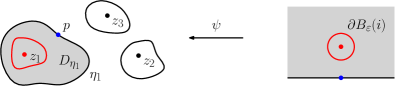
Figure 4: Illustration for Lemma 5.8 and the proof of Proposition 5.4. The region $D_{\eta_{1}}$ surrounded by $\eta_{1}$ is colored grey. Both $(D_{\eta_{1}},\phi,z_{1},p)$ and $(\mathbbm{H},X,0,i)$ are embeddings of $\mathcal{D}_{1}$, which are related by $\psi$. The domain $\mathbbm{C}_{\eta_{1},p,\varepsilon}$ equals $\mathbbm{C}\setminus\psi(B_{\varepsilon}(i))$, the region outside the red curve on the left.

Proof of Proposition 5.4.

In the setting of Lemma 5.8 with $\alpha=\gamma$, by Lemma 5.3 the law of $(\phi,\eta_{1},\eta_{2},\eta_{3},p)$ is $\mathrm{Harm_{z_{1},\eta_{1}}}(dp)\,\mathrm{LF}_{\mathbbm{C}}^{(\gamma,z_{1}),(\gamma,z_{2}),(\gamma,z_{3})}(d\phi)\,\mathsf{m}_{3}(d\eta_{1},d\eta_{2},d\eta_{3})$, where $\mathrm{Harm}_{z_{1},\eta_{1}}$ means the harmonic measure on $\eta_{1}$ viewed from $z_{1}$. Therefore Lemma 5.8 with $\alpha=\gamma$ can be written as

$$\mathrm{LF}_{\mathbbm{C}}^{(\gamma,z_{1}),(\gamma,z_{2}),(\gamma,z_{3})}(d\phi)\,\mathrm{Harm_{z_{1},\eta_{1}}}(dp)\,\mathsf{m}_{3}(d\eta_{1},d\eta_{2},d\eta_{3})=\int_{0}^{\infty}\ell\mathrm{LF}_{\mathbbm{H}}^{(\gamma,i)}(\ell)\times\mathfrak{M}_{\ell}^{\bullet}d\ell,$$ (5.8)

in the sense that $(\phi,\eta_{1},\eta_{2},\eta_{3},p)$ and $(X,\mathcal{D}^{c}_{1})$ determine each other, and the two sides of (5.8) give the laws of $(\phi,\eta_{1},\eta_{2},\eta_{3},p)$ and $(X,\mathcal{D}^{c}_{1})$, respectively.

Recall the notations in Lemma 5.6. For $\varepsilon\in(0,\frac{1}{4})$, for any nonnegative measurable function $f$ of $\phi|_{\mathbbm{C}_{\eta_{1},p,\varepsilon}}$, and any nonnegative measure function $g$ of $(\eta_{1},\eta_{2},\eta_{3})$, we get from (5.8) that

$$\int f(\phi|_{\mathbbm{C}_{\eta_{1},p,\varepsilon}})g(\eta_{1},\eta_{2},\eta_{3})\varepsilon^{\frac{1}{2}(\alpha^{2}-\gamma^{2})}e^{(\alpha-\gamma)X_{\varepsilon}(i)}\mathrm{LF}_{\mathbbm{C}}^{(\gamma,z_{1}),(\gamma,z_{2}),(\gamma,z_{3})}(d\phi)\,\mathrm{Harm_{z_{1},\eta_{1}}}(dp)\,\mathsf{m}_{3}(d\eta_{1},d\eta_{2},d\eta_{3})$$

$$=\int_{0}^{\infty}\mathopen{}\mathclose{{}\left(\int f(\phi|_{\mathbbm{C}_{\eta_{1},p,\varepsilon}})g(\eta_{1},\eta_{2},\eta_{3})\varepsilon^{\frac{1}{2}(\alpha^{2}-\gamma^{2})}e^{(\alpha-\gamma)X_{\varepsilon}(i)}\ell\mathrm{LF}_{\mathbbm{H}}^{(\gamma,i)}(\ell)\times\mathfrak{M}_{\ell}^{\bullet}}\right)d\ell.$$ (5.9)

Recall that $\mathsf{m}_{3}^{\alpha,\gamma,\gamma}=\mathopen{}\mathclose{{}\left(\frac{1}{2}\mathrm{CR}(\eta_{1},z_{1})}\right)^{-\frac{\alpha^{2}}{2}+Q\alpha-2}\mathsf{m}_{3}$. By Lemma 5.6, the left side of (5.9) equals

$$\int fg\mathopen{}\mathclose{{}\left(\frac{1}{2}\mathrm{CR}(\eta_{1},z_{1})}\right)^{-\frac{\alpha^{2}}{2}+Q\alpha-2}\mathrm{LF}_{\mathbbm{C}}^{(\alpha,z_{1}),(\gamma,z_{2}),(\gamma,z_{3})}(d\phi)\,\mathrm{Harm_{z_{1},\eta_{1}}}(dp)\,\mathsf{m}_{3}(d\eta_{1},d\eta_{2},d\eta_{3})$$

$$= \int fg\mathrm{LF}_{\mathbbm{C}}^{(\alpha,z_{1}),(\gamma,z_{2}),(\gamma,z_{3})}(d\phi)\mathrm{Harm_{z_{1},\eta_{1}}}(dp)\,\mathsf{m}_{3}^{\alpha,\gamma,\gamma}\,(d\eta_{1},d\eta_{2},d\eta_{3}).$$ (5.10)

Here we write $f=f(\phi|_{\mathbbm{C}_{\eta_{1},p,\varepsilon}})$ and $g=g(\eta_{1},\eta_{2},\eta_{3})$ to ease the notation.

By Lemma 5.5, the right side of (5.9) equals

$$\int_{0}^{\infty}\mathopen{}\mathclose{{}\left(\int fg\ell\mathrm{LF}_{\mathbbm{H}}^{(\alpha,i)}(\ell)\times\mathfrak{M}_{\ell}^{\bullet}}\right)d\ell.$$ (5.11)

Since $\varepsilon,f,g$ are arbitrary, comparing (5.10) and (5.11) we get in the same sense as in (5.8) that

$$\mathrm{LF}_{\mathbbm{C}}^{(\alpha,z_{1}),(\gamma,z_{2}),(\gamma,z_{3})}(d\phi)\mathrm{Harm_{z_{1},\eta_{1}}}(dp)\,\mathsf{m}_{3}^{\alpha,\gamma,\gamma}(d\eta_{1},d\eta_{2},d\eta_{3})=\int_{0}^{\infty}\ell\mathrm{LF}_{\mathbbm{H}}^{(\alpha,i)}(\ell)\times\mathfrak{M}_{\ell}^{\bullet}d\ell.$$

Forgetting about the point $p$ we get Proposition 5.4. ∎

Proof of Theorem 5.2.

The case $(\alpha_{1},\alpha_{2},\alpha_{3})=(\alpha,\gamma,\gamma)$ was proved in Proposition 5.4 by reweighting from the $(\gamma,\gamma,\gamma)$ case. The exact same argument in Lemma 5.6 gives the following extension:

$$\int f(\phi|_{\mathbbm{C}_{\eta_{1},p,\varepsilon}})\times\varepsilon^{\frac{1}{2}(\alpha^{2}-\alpha_{1}^{2})}e^{(\alpha-\alpha_{1})X_{\varepsilon}(i)}\,d\mathrm{LF}_{\mathbbm{C}}^{(\alpha_{1},z_{1}),(\alpha_{2},z_{2}),(\alpha_{3},z_{3})}$$

$$= \int f(\phi|_{\mathbbm{C}_{\eta_{1},p,\varepsilon}})\mathopen{}\mathclose{{}\left(\frac{1}{2}\mathrm{CR}(\eta_{1},z_{1})}\right)^{-\frac{\alpha_{1}^{2}}{2}+Q\alpha_{1}-2}\mathrm{LF}_{\mathbbm{C}}^{(\alpha,z_{1}),(\alpha_{2},z_{2}),(\alpha_{3},z_{3})}.$$ (5.12)

By symmetry (5.12) holds if the roles of $z_{1},z_{2},z_{3}$ are permutated. This allows us to obtain the general $(\alpha_{1},\alpha_{2},\alpha_{3})$ case from the $(\gamma,\gamma,\gamma)$ case by reweighing around the three points sequentially. ∎

5.2 Matching the quantum area: proof of Theorem 1.2

Theorem 1.2 is an immediate consequence of Lemma 5.1 and the following proposition.

Proposition 5.9.

Fix $(z_{1},z_{2},z_{3})=(0,1,e^{i\pi/3})$. There is a constant $C=C(\gamma)\in(0,\infty)$ such that for $\alpha_{1},\alpha_{2},\alpha_{3}\in(Q-\frac{\gamma}{4},Q)$, and $\mathsf{m}_{3}^{\alpha_{1},\alpha_{2},\alpha_{3}}$ as defined in (5.1) we have

$$\mathopen{}\mathclose{{}\left(\mathrm{LF}_{\mathbbm{C}}^{(\alpha_{i},z_{i})_{3}}\times\mathsf{m}_{3}^{\alpha_{1},\alpha_{2},\alpha_{3}}}\right)[e^{-\mu_{\phi}(\mathbbm{C})}]=C\prod_{i=1}^{3}\frac{2^{\alpha_{i}^{2}/2-Q\alpha_{i}}\Gamma(\frac{\gamma\alpha_{i}}{2}-\frac{\gamma^{2}}{4})}{\Gamma(\frac{2}{\gamma}(Q-\alpha_{i}))\cos(\frac{2\pi}{\gamma}(Q-\alpha_{i}))}\mathopen{}\mathclose{{}\left(\frac{\pi\Gamma(\frac{\gamma^{2}}{4})}{\Gamma(1-\frac{\gamma^{2}}{4})}}\right)^{-\frac{\alpha_{i}}{\gamma}}.$$ (5.13)

Proof.

Recall $\mathrm{QP}_{3}(\ell_{1},\ell_{2},\ell_{3})[e^{-A}]$ from Theorem 4.2. Recall $\mathcal{M}_{1}^{\mathrm{disk}}(\alpha_{i};\ell_{i})[e^{-A_{i}}]$ from Theorem 2.16, where $A_{i}$ is the quantum area of a sample from $\mathcal{M}_{1}^{\mathrm{disk}}(\alpha_{i};\ell_{i})$. By Theorem 5.2, for some $\gamma$-dependent constants $C_{1},C_{2},C_{3}$, we have that $\mathopen{}\mathclose{{}\left(\mathrm{LF}_{\mathbbm{C}}^{(\alpha_{i},z_{i})_{3}}\times\mathsf{m}_{3}^{\alpha_{1},\alpha_{2},\alpha_{3}}}\right)[e^{-\mu_{\phi}(\mathbbm{C})}]$ equals

$$C_{1} \iiint_{0}^{\infty}\ell_{1}\ell_{2}\ell_{3}\mathrm{QP}_{3}(\ell_{1},\ell_{2},\ell_{3})[e^{-A}]\prod_{i=1}^{3}\mathcal{M}_{1}^{\mathrm{disk}}(\alpha_{i};\ell_{i})[e^{-A_{i}}]\,d\ell_{1}\,d\ell_{2}\,d\ell_{3}$$

$$=C_{2}\prod_{i=1}^{3}\frac{\overline{U}(\alpha_{i})(4\sin(\frac{\pi\gamma^{2}}{4}))^{\alpha_{i}/\gamma}}{2^{\alpha_{i}^{2}/2}\Gamma(\frac{2}{\gamma}(Q-\alpha_{i}))}\int_{0}^{\infty}\frac{1}{\sqrt{\ell_{i}}}e^{-\ell_{i}\sqrt{\frac{1}{\sin(\pi\gamma^{2}/4)}}}K_{\frac{2}{\gamma}(Q-\alpha_{i})}\mathopen{}\mathclose{{}\left(\ell_{i}\sqrt{\frac{1}{\sin(\pi\gamma^{2}/4)}}}\right)\,d\ell_{i}$$

$$=C_{3}\prod_{i=1}^{3}\frac{\overline{U}(\alpha_{i})(4\sin(\frac{\pi\gamma^{2}}{4}))^{\alpha_{i}/\gamma}}{2^{\alpha_{i}^{2}/2}\Gamma(\frac{2}{\gamma}(Q-\alpha_{i}))\cos(\frac{2\pi}{\gamma}(Q-\alpha_{i}))},$$

where $\overline{U}$ is as in (2.4) and (2.7) is used to evaluate the integral on the second line. Expanding $\overline{U}(\alpha_{i})$ from (2.4) and substituting $\sin(\frac{\pi\gamma^{2}}{4})$ by $\frac{\pi}{\Gamma(\frac{\gamma^{2}}{4})\Gamma(1-\frac{\gamma^{2}}{4})}$, we get (5.13). ∎

Proof of Theorem 1.2.

We divide the proof into four cases depending on the parameter range.

Case I: $\kappa<4$ and $\lambda_{i}\in(\frac{3\kappa}{32}-1+\frac{2}{\kappa},\frac{\kappa}{8}-1+\frac{2}{\kappa})$ for all $i=1,2,3$. In this case we can find $\alpha_{i}\in(Q-\frac{\gamma}{4},Q)$ satisfying $\lambda_{i}=-\frac{\alpha_{i}^{2}}{2}+Q\alpha_{i}-2$ for each $i$. Comparing Lemma 5.1 and Proposition 5.9 yields that for some $\gamma$-dependent constant $C(\gamma)$ we have

$${C^{\operatorname{CLE}}_{\kappa}(\lambda_{1},\lambda_{2},\lambda_{3})}=\frac{C(\gamma)}{C_{\gamma}^{\mathrm{DOZZ}}(\alpha_{1},\alpha_{2},\alpha_{3})}\prod_{i=1}^{3}\frac{\Gamma(\frac{\gamma\alpha_{i}}{2}-\frac{\gamma^{2}}{4})}{\Gamma(\frac{2}{\gamma}(Q-\alpha_{i}))\cos(\frac{2\pi}{\gamma}(Q-\alpha_{i}))}\mathopen{}\mathclose{{}\left(\frac{\pi\Gamma(\frac{\gamma^{2}}{4})}{\Gamma(1-\frac{\gamma^{2}}{4})}}\right)^{-\frac{\alpha_{i}}{\gamma}}.$$

Now we can evaluate $C(\gamma)$ by setting $\alpha_{1}=\alpha_{2}=\alpha_{3}=\gamma$, in which case $\lambda_{i}=0$ and $C_{\kappa}^{\operatorname{CLE}}(0,0,0)=1$. This gives (1.3) for ${C^{\operatorname{CLE}}_{\kappa}(\lambda_{1},\lambda_{2},\lambda_{3})}$ and (1.4) for the factor $N_{\gamma}(\alpha)$.

For the next two cases set $(z_{1},z_{2},z_{3})=(0,1,e^{i\pi/3})$ so that $C_{\kappa}^{\operatorname{CLE}}(\lambda_{1},\lambda_{2},\lambda_{3})=\mathbbm{E}[\prod_{i=1}^{3}(\mathrm{CR}(\eta_{i},z_{i}))^{\lambda_{i}}]$. Since the distance between $z_{i}$ and $\eta_{i}$ is less than $1$, Koebe 1/4 theorem yields $\frac{1}{4}\mathrm{CR}(\eta_{i},z_{i})\leq 1$. Thus $\mathbbm{E}[\prod_{i=1}^{3}(\frac{1}{4}\mathrm{CR}(\eta_{i},z_{i}))^{\lambda_{i}}]\leq\mathbbm{E}[\prod_{i=1}^{3}(\frac{1}{4}\mathrm{CR}(\eta_{i},z_{i}))^{\widetilde{\lambda}_{i}}]$ for any real $\lambda_{i},\widetilde{\lambda}_{i}$ such that $\lambda_{i}\geq\widetilde{\lambda}_{i}$. Namely

$$4^{-\lambda_{1}-\lambda_{2}-\lambda_{3}}C_{\kappa}^{\operatorname{CLE}}(\lambda_{1},\lambda_{2},\lambda_{3})\leq 4^{-\widetilde{\lambda}_{1}-\widetilde{\lambda}_{2}-\widetilde{\lambda}_{3}}C_{\kappa}^{\operatorname{CLE}}(\widetilde{\lambda}_{1},\widetilde{\lambda}_{2},\widetilde{\lambda}_{3}).$$ (5.14)

Case II: $\kappa<4$ and all $\lambda_{i}>\frac{3\kappa}{32}-1+\frac{2}{\kappa}$. By (5.14) on $\{(\lambda_{1},\lambda_{2},\lambda_{3})\in\mathbbm{C}^{3}:\operatorname{Re}\lambda_{i}>\frac{3\kappa}{32}-1+\frac{2}{\kappa}\}$, the function ${C^{\operatorname{CLE}}_{\kappa}(\lambda_{1},\lambda_{2},\lambda_{3})}$ is finite, hence analytic. On the other hand, the right hand side of (1.3) is an explicit meromorphic function in $(\alpha_{1},\alpha_{2},\alpha_{3})$. Now Case II follows from Case I.

Case III: $\kappa<4$ and $\lambda_{i}\leq\frac{3\kappa}{32}-1+\frac{2}{\kappa}$ for some $i$. We will show that ${C^{\operatorname{CLE}}_{\kappa}(\lambda_{1},\lambda_{2},\lambda_{3})}=\infty$ in this case. By the monotonicity (5.14) and symmetry, it suffices to prove $C_{\kappa}^{\operatorname{CLE}}(\lambda_{1},\lambda_{2},\lambda_{3})=\infty$ for $\lambda_{1}\leq\frac{3\kappa}{32}-1+\frac{2}{\kappa}$ and $\lambda_{2},\lambda_{3}>\frac{3\kappa}{32}-1+\frac{2}{\kappa}$. For $\lambda>\frac{3\kappa}{32}-1+\frac{2}{\kappa}$ we have

$$4^{-\lambda_{1}-\lambda_{2}-\lambda_{3}}C_{\kappa}^{\operatorname{CLE}}(\lambda_{1},\lambda_{2},\lambda_{3})>4^{-\lambda-\lambda_{2}-\lambda_{3}}C_{\kappa}^{\operatorname{CLE}}(\lambda,\lambda_{2},\lambda_{3}),$$

Suppose $(\alpha,\alpha_{2},\alpha_{3})\in(Q-\frac{\gamma}{4},Q)^{3}$ correspond to $(\lambda,\lambda_{2},\lambda_{3})$. Then $\lambda\downarrow\frac{3\kappa}{32}-1+\frac{2}{\kappa}$ means $\alpha\downarrow Q-\frac{\gamma}{4}$. Recall the explicit formula for $C_{\kappa}^{\operatorname{CLE}}(\lambda,\lambda_{2},\lambda_{3})$ in (1.3) proven in Case II. Since $\lim_{\alpha\downarrow Q-\frac{\gamma}{4}}N_{\gamma}(\alpha)=\infty$ and $C_{\gamma}^{\mathrm{DOZZ}}(\alpha,\alpha_{2},\alpha_{3})\in(0,\infty)$ as $(\alpha,\alpha_{2},\alpha_{3})$ satisfies the Seiberg bounds (2.2), we must have $C_{\kappa}^{\operatorname{CLE}}(\lambda,\lambda_{2},\lambda_{3})\rightarrow\infty$ as $\lambda\downarrow\frac{3\kappa}{32}-1+\frac{2}{\kappa}$. Therefore $C_{\kappa}^{\operatorname{CLE}}(\lambda_{1},\lambda_{2},\lambda_{3})=\infty$ as desired.

Case IV: $\kappa=4$. This follows from Lemma A.5 via the continuity as $\kappa\uparrow 4$. ∎

6 Electrical thickness of the SLE loop via conformal welding

In this section we prove Theorem 1.3. We will work on the horizontal cylinder $\mathcal{C}=\mathbbm{R}\times[0,2\pi]/{\sim}$ with $x\sim x+2\pi i$ for $x\in\mathbbm{R}$. Recall the shape measure $\mathcal{L}_{\kappa}$ of $\operatorname{SLE}^{\mathrm{loop}}_{\kappa}$. Let $\mathcal{L}_{\kappa}(\mathcal{C})$ be the pullback of $\mathcal{L}_{\kappa}$ under the map $z\mapsto e^{-z}$, which is a probability measure on loops $\eta$ in $\mathcal{C}$ separating $\pm\infty$ and satisfying $\max_{z\in\eta}\operatorname{Re}z=0$. For a loop $\eta$ sampled from $\mathcal{L}_{\kappa}(\mathcal{C})$, we write $\vartheta(\eta)$ for the electrical thickness of $\exp(\eta)$, namely $-\log\mathrm{CR}(\exp(\eta),0)-\log\mathrm{CR}(\exp(-\eta),0)$. Then Theorem 1.3 is equivalent to

$$\mathbbm{E}[e^{\lambda\vartheta(\eta)}]=\mathopen{}\mathclose{{}\left\{\begin{array}[]{ll}\frac{\sin(\pi(1-\kappa/4))}{\pi(1-\kappa/4)}\frac{\pi\sqrt{(1-\kappa/4)^{2}+\lambda\kappa/2}}{\sin(\pi\sqrt{(1-\kappa/4)^{2}+\lambda\kappa/2})}&\mbox{if }\lambda<1-\frac{\kappa}{8}.\\ \infty&\mbox{if }\lambda\geq 1-\frac{\kappa}{8}\end{array}}\right.$$ (6.1)

Consider $\alpha<Q$ and set $\lambda=\frac{\alpha^{2}}{2}-Q\alpha+2$. Let $\mathcal{L}_{\kappa}^{\alpha}$ be defined by the following reweighting of $\mathcal{L}_{\kappa}(\mathcal{C})$:

$$\frac{d\mathcal{L}_{\kappa}^{\alpha}}{d\mathcal{L}_{\kappa}(\mathcal{C})}(\eta)=(\frac{1}{4}\mathrm{CR}(\exp(\eta),0)\mathrm{CR}(\exp(-\eta),0))^{-\frac{\alpha^{2}}{2}+Q\alpha-2}=2^{2\lambda}e^{\lambda\vartheta(\eta)}.$$ (6.2)

Then proving Theorem 1.3 amounts to computing the total mass $|\mathcal{L}_{\kappa}^{\alpha}|$. Similarly as in the proof of Theorem 1.2 in Section 5, we need a conformal welding result, Proposition 6.2, which involves $\mathcal{L}_{\kappa}^{\alpha}$. It is a generalization of Proposition 2.20 where marked points have $\alpha$-singularities. To state it we first recall the $\alpha$-generalization of the two-pointed quantum sphere; see e.g. [AHS20, Section 2].

Definition 6.1.

For $\gamma\in(0,2)$, let $(B_{s})_{s\geq 0}$ be a standard Brownian motion conditioned on $B_{s}-(Q-\alpha)s<0$ for all $s>0$, and $(\widetilde{B}_{s})_{s\geq 0}$ an independent copy of $(B_{s})_{s\geq 0}$. Let

$$Y_{t}=\mathopen{}\mathclose{{}\left\{\begin{array}[]{ll}B_{t}-(Q-\alpha)t&\mbox{if }t\geq 0\\ \widetilde{B}_{-t}+(Q-\alpha)t&\mbox{if }t<0\end{array}}\right.$$

Let $h^{1}(z)=Y_{\operatorname{Re}z}$ for each $z\in\mathcal{C}$. Let $h^{2}_{\mathcal{C}}$ be independent of $h^{1}$ and have the law of the lateral component of the GFF on $\mathcal{C}$. Let $\hat{h}=h^{1}+h^{2}_{\mathcal{C}}$. Let $\mathbf{c}\in\mathbbm{R}$ be sampled from $\frac{\gamma}{2}e^{2(\alpha-Q)c}dc$ independent of $\hat{h}$. Let $\mathcal{M}_{2}^{\mathrm{sph}}(\alpha)$ be the infinite measure describing the law of the decorated quantum surface $(\mathcal{C},\hat{h}+\mathbf{c},-\infty,+\infty)/{\sim_{\gamma}}$.

Consider $\kappa\in(0,4)$ and $\gamma=\sqrt{\kappa}$. Sample a pair $(\eta,\mathbf{t})$ from $\mathcal{L}_{\kappa}^{\alpha}\times dt$ where $dt$ is the Lebesgue measure on $\mathbbm{R}$. Let $\operatorname{SLE}_{\kappa}^{\mathrm{sep},\alpha}$ be the law of the translated loop $\eta+\mathbf{t}$. Let $\mathbb{F}$ be the law of $\hat{h}+\mathbf{c}$ as in Definition 6.1, so that the law of $(\mathcal{C},\hat{h}+\mathbf{c},-\infty,+\infty)/{\sim_{\gamma}}$ is $\mathcal{M}_{2}^{\mathrm{sph}}(\alpha)$. Now sample $(h,\eta)$ from $\mathbb{F}\times\operatorname{SLE}_{\kappa}^{\mathrm{sep},\alpha}$ and write $\mathcal{M}_{2}^{\mathrm{sph}}(\alpha)\otimes\operatorname{SLE}_{\kappa}^{\mathrm{sep,\alpha}}$ as the law of $(\mathcal{C},h,\eta,-\infty,+\infty)/{\sim_{\gamma}}$. We are now ready to state the conformal welding result needed for the proof of Theorem 1.3.

Proposition 6.2.

For $\alpha\in(\frac{\gamma}{2},Q)$ and some $\gamma$-dependent constant $C\in(0,\infty)$ we have

$$C(Q-\alpha)^{2}\mathcal{M}_{2}^{\mathrm{sph}}(\alpha)\otimes\operatorname{SLE}_{\kappa}^{\mathrm{sep},\alpha}=\int_{0}^{\infty}\ell\cdot\mathrm{Weld}(\mathcal{M}_{1}^{\mathrm{disk}}(\alpha;\ell),\mathcal{M}_{1}^{\mathrm{disk}}(\alpha;\ell))\,d\ell,$$ (6.3)

where $\mathrm{Weld}(\mathcal{M}_{1}^{\mathrm{disk}}(\alpha;\ell),\mathcal{M}_{1}^{\mathrm{disk}}(\alpha;\ell))$ is defined as $\mathrm{Weld}(\mathrm{QD}_{1,0}(\ell),\mathrm{QD}_{1,0}(\ell))$ in Proposition 2.20.

We postpone the proof of Proposition 6.2 to Section 6.1 and proceed to the proof of Theorem 1.3. Similarly as in the proof of Theorem 1.2, we would like to evaluate the average of $e^{-A}$ on both sides of (6.3) and compare the expressions to obtain $|\mathcal{L}^{\alpha}_{\kappa}|$. However, since $\mathcal{M}_{2}^{\mathrm{sph}}(\alpha)\otimes\operatorname{SLE}_{\kappa}^{\mathrm{sep},\alpha}[e^{-A}]=\infty$, we have to consider an alternative observable. Note that $\mathcal{M}_{2}^{\mathrm{sph}}(\alpha)\otimes\operatorname{SLE}_{\kappa}^{\mathrm{sep},\alpha}$ is a measure on quantum surfaces decorated by two (ordered) marked points and a loop separating them. The loop separates the quantum surface into two connected components. For $0<\varepsilon<\delta$, let $E_{\delta,\varepsilon}$ be the event that the connected component containing the first marked point has quantum area at least 1 and the loop has quantum length in $(\varepsilon,\delta)$. We use the size of $E_{\delta,\varepsilon}$ as our obervable, whose asymptotic is easy to obtain using Proposition 6.2.

Lemma 6.3.

Let $\alpha\in(\frac{\gamma}{2},Q)$. Recall $\overline{U}(\alpha)$ from Proposition 2.10. With $C$ from Proposition 6.2 and an error term $o_{\delta,\varepsilon}(1)$ satisfying $\lim_{\delta\to 0}\limsup_{\varepsilon\to 0}|o_{\delta,\varepsilon}(1)|=0$, we have

$$\mathcal{M}_{2}^{\mathrm{sph}}(\alpha)\otimes\operatorname{SLE}_{\kappa}^{\mathrm{sep},\alpha}[E_{\delta,\varepsilon}]=\frac{1}{C(Q-\alpha)^{2}}\times\frac{(1+o_{\delta,\varepsilon}(1))\log\varepsilon^{-1}}{\frac{2}{\gamma}(Q-\alpha)\Gamma(\frac{2}{\gamma}(Q-\alpha))}\mathopen{}\mathclose{{}\left(\frac{2}{\gamma}2^{-\frac{\alpha^{2}}{2}}\overline{U}(\alpha)}\right)^{2}\mathopen{}\mathclose{{}\left(4\sin\frac{\pi\gamma^{2}}{4}}\right)^{-\frac{2}{\gamma}(Q-\alpha)}.$$

Proof.

By Proposition 6.2, $C(Q-\alpha)^{2}\mathcal{M}_{2}^{\mathrm{sph}}(\alpha)\otimes\operatorname{SLE}_{\kappa}^{\mathrm{sep},\alpha}[E_{\delta,\varepsilon}]$ equals the mass of $E_{\delta,\varepsilon}$ under the measure $\int_{0}^{\infty}\ell\cdot\mathrm{Weld}(\mathcal{M}_{1}^{\mathrm{disk}}(\alpha;\ell),\mathcal{M}_{1}^{\mathrm{disk}}(\alpha;\ell))\,d\ell$. This mass can be expressed as

$$\int_{\varepsilon}^{\delta}\ell\cdot\mathopen{}\mathclose{{}\left|\mathcal{M}_{1}^{\mathrm{disk}}(\alpha;\ell)}\right|\mathcal{M}_{1}^{\mathrm{disk}}(\alpha;\ell)[A>1]\,d\ell=\int_{\varepsilon}^{\delta}\ell\mathopen{}\mathclose{{}\left|\mathcal{M}_{1}^{\mathrm{disk}}(\alpha;\ell)}\right|^{2}\mathcal{M}_{1}^{\mathrm{disk}}(\alpha;\ell)^{\#}[A>1]\;d\ell,$$ (6.4)

where $A$ is the quantum area of a sample from $\mathcal{M}_{1}^{\mathrm{disk}}(\alpha;\ell)$. From the scaling relation between quantum area and length, and the explicit density of $A$ under $\mathcal{M}_{1}^{\mathrm{disk}}(\alpha;1)^{\#}$ given by the FZZ formula Theorem 2.16, we see that

$$\mathcal{M}_{1}^{\mathrm{disk}}(\alpha;\ell)^{\#}[A>1]=\mathcal{M}_{1}^{\mathrm{disk}}(\alpha;1)^{\#}[A>\ell^{-2}]=\frac{1+o_{\ell}(1)}{\frac{2}{\gamma}(Q-\alpha)\Gamma(\frac{2}{\gamma}(Q-\alpha))}\mathopen{}\mathclose{{}\left(\frac{\ell^{2}}{4\sin\frac{\pi\gamma^{2}}{4}}}\right)^{\frac{2}{\gamma}(Q-\alpha)}\textrm{ as }\ell\to 0.$$

By Proposition 2.10, $|\mathcal{M}_{1}^{\mathrm{disk}}(\alpha;\ell)|=\frac{2}{\gamma}2^{-\frac{\alpha^{2}}{2}}\overline{U}(\alpha)\ell^{\frac{2}{\gamma}(\alpha-Q)-1}$. Therefore the right side of (6.4) equals

$$\frac{1}{\frac{2}{\gamma}(Q-\alpha)\Gamma(\frac{2}{\gamma}(Q-\alpha))}\mathopen{}\mathclose{{}\left(\frac{2}{\gamma}2^{-\frac{\alpha^{2}}{2}}\overline{U}(\alpha)}\right)^{2}\mathopen{}\mathclose{{}\left(4\sin\frac{\pi\gamma^{2}}{4}}\right)^{-\frac{2}{\gamma}(Q-\alpha)}\int_{\varepsilon}^{\delta}\ell^{-1}(1+o_{\ell}(1))\,d\ell.$$

Writing $\int_{\varepsilon}^{\delta}\ell^{-1}(1+o_{\ell}(1))\,d\ell$ as $(1+o_{\delta,\varepsilon}(1))\log\varepsilon^{-1}$, we have $\lim_{\delta\to 0}\limsup_{\varepsilon\to 0}|o_{\delta,\varepsilon}(1)|=0$ as desired. ∎

Given Lemma 6.3, the following proposition is the key to our proof of Theorem 1.3. It gives the size of $E_{\delta,\varepsilon}$ in terms of $|\mathcal{L}_{\kappa}^{\alpha}|$ and the reflection coefficient for LCFT.

Proposition 6.4.

Let $\alpha\in(\frac{\gamma}{2},Q)$. With an error term $o_{\delta,\varepsilon}(1)$ satisfying $\lim_{\delta\to 0}\limsup_{\varepsilon\to 0}|o_{\delta,\varepsilon}(1)|=0$, we have

$$(\mathcal{M}_{2}^{\mathrm{sph}}(\alpha)\otimes\operatorname{SLE}_{\kappa}^{\mathrm{sep},\alpha})[E_{\delta,\varepsilon}]=(1+o_{\delta,\varepsilon}(1))\frac{\overline{R}(\alpha)}{2(Q-\alpha)^{2}}|\mathcal{L}_{\kappa}^{\alpha}|\log\varepsilon^{-1},$$

where $\overline{R}(\alpha)$ is the unit-volume reflection coefficient for LCFT on the sphere [KRV17, RV19]:

$$\overline{R}(\alpha)=-\mathopen{}\mathclose{{}\left(\frac{\pi\Gamma(\frac{\gamma^{2}}{4})}{\Gamma(1-\frac{\gamma^{2}}{4})}}\right)^{\frac{2}{\gamma}(Q-\alpha)}\frac{1}{\frac{2}{\gamma}(Q-\alpha)}\frac{\Gamma(-\frac{\gamma}{2}(Q-\alpha))}{\Gamma(\frac{\gamma}{2}(Q-\alpha))\Gamma(\frac{2}{\gamma}(Q-\alpha))}.$$ (6.5)

We postpone the proof of Proposition 6.4 to Section 6.2 and proceed to prove Theorem 1.3.

Proposition 6.5.

There exists a $\gamma$-dependent constant $C\in(0,\infty)$ such that

$$2^{-\alpha^{2}+2Q\alpha}|\mathcal{L}_{\kappa}^{\alpha}|=C\frac{\frac{\gamma}{2}(Q-\alpha)}{\sin(\frac{\gamma\pi}{2}(Q-\alpha))}\quad\textrm{for all }\alpha\in(\frac{\gamma}{2},Q).$$ (6.6)

Proof.

By Lemma 6.3 and Proposition 6.4, we get

$$\overline{R}(\alpha)|\mathcal{L}_{\kappa}^{\alpha}|=\frac{C^{\prime}}{(Q-\alpha)\Gamma(\frac{2}{\gamma}(Q-\alpha))}\mathopen{}\mathclose{{}\left(2^{-\frac{\alpha^{2}}{2}}\overline{U}(\alpha)}\right)^{2}\mathopen{}\mathclose{{}\left(4\sin\frac{\pi\gamma^{2}}{4}}\right)^{-\frac{2}{\gamma}(Q-\alpha)}$$

for some $\gamma$-dependent constant $C^{\prime}$. Plugging in $\overline{R}(\alpha)$ and $\overline{U}(\alpha)$ from (6.5) and (2.4), and simplifying via the identities $\Gamma(z+1)=z\Gamma(z)$ and $\Gamma(1-z)\Gamma(z)=\frac{\pi}{\sin(\pi z)}$, we arrive at (6.6). ∎

Proof of Theorem 1.3.

We break the proof of (6.1) hence Theorem 1.3, into three cases.

Case I: $\kappa<4$ and $\lambda\in(1-\frac{\kappa}{8}-\frac{2}{\kappa},1-\frac{\kappa}{8})$. Set $\alpha=Q-\sqrt{Q^{2}-4+2\lambda}$. Then $\alpha\in(\frac{\gamma}{2},Q)$ in this case. Since $\lambda=\frac{\alpha^{2}}{2}-Q\alpha+2$, by (6.2) and Proposition 6.5 we have

$$\mathbbm{E}[e^{\lambda\vartheta(\eta)}]=2^{-2\lambda}|\mathcal{L}_{\kappa}^{\alpha}|=C\frac{\frac{\gamma}{2}(Q-\alpha)}{\sin(\frac{\gamma\pi}{2}(Q-\alpha))}=C\frac{\sqrt{(1-\frac{\kappa}{4})^{2}+\frac{\lambda\kappa}{2}}}{\sin(\pi\sqrt{(1-\frac{\kappa}{4})^{2}+\frac{\lambda\kappa}{2}})}$$

for some $\gamma$-dependent constant $C$. Since $\kappa\in(0,4)$, we have $0\in(1-\frac{\kappa}{8}-\frac{2}{\kappa},1-\frac{\kappa}{8})$. Thus we can obtain the value of $C$ by considering $1=\mathbbm{E}[e^{0}]=\frac{C(1-\kappa/4)}{\sin(\pi(1-\kappa/4))}$. This yields (6.1) in this case.

Case II: $\kappa<4$ and $\lambda\in\mathbbm{R}$. Since $\vartheta(\eta)\geq 0$, the function $\lambda\mapsto\mathbbm{E}[e^{\lambda\vartheta(\eta)}]$ is increasing. Thus for $\lambda<0$ we have $\mathbbm{E}[e^{\lambda\vartheta(\eta)}]\leq\mathbbm{E}[e^{0\cdot\vartheta(\eta)}]=1$. Since $1-\frac{\kappa}{8}-\frac{2}{\kappa}<0$ we can use analytic continuation to extend (6.1) from $\lambda\in(1-\frac{\kappa}{8}-\frac{2}{\kappa},1-\frac{\kappa}{8})$ to $\lambda\in(-\infty,1-\frac{\kappa}{8})$. On the other hand, for any $\lambda\geq 1-\frac{\kappa}{8}$ we have $\mathbbm{E}[e^{\lambda\vartheta(\eta)}]\geq\lim_{\lambda^{\prime}\uparrow 1-\frac{\kappa}{8}}\mathbbm{E}[e^{\lambda^{\prime}\vartheta(\eta)}]$, which equals $\infty$ using the explicit formula of $\mathbbm{E}[e^{\lambda^{\prime}\vartheta(\eta)}]$.

Case III: $\kappa=4$. By Lemma A.4, $\vartheta(\eta_{\kappa})\to\vartheta(\eta_{4})$ in law as $\kappa\uparrow 4$, where $\eta_{\kappa}$ is a sample from $\mathcal{L}_{\kappa}$. Fix $\lambda<\frac{1}{2}$ and $\lambda^{\prime}\in(\lambda,\frac{1}{2})$. Since $\mathbbm{E}[e^{\lambda\vartheta(\eta_{\kappa})}]\leq\mathbbm{E}[e^{\lambda^{\prime}\vartheta(\eta_{\kappa})}]$ and $\mathbbm{E}[e^{\lambda^{\prime}\vartheta(\eta_{\kappa})}]$ is uniformly bounded in $\kappa\in[3,4)$, the family $\{e^{\lambda\vartheta(\eta_{\kappa})}:\kappa\in[3,4)\}$ is uniformly integrable. Therefore $\lim_{\kappa\uparrow 4}\mathbbm{E}[e^{\lambda\vartheta(\eta_{\kappa})}]=\mathbbm{E}[e^{\lambda\vartheta(\eta_{4})}]$ as desired. For $\lambda\geq\frac{1}{2}$, the same argument as in Case II gives $\mathbbm{E}[e^{\lambda\vartheta(\eta)}]=\infty$. ∎

It remains to prove Propositions 6.2 and 6.4. The common starting point of the proofs is the relation between $\mathcal{M}_{2}^{\mathrm{sph}}(\alpha)$ and the Liouville field on $\mathcal{C}$ that we now recall from [AHS21].

Definition 6.6.

Let $P_{\mathcal{C}}$ be the law of the GFF on the cylinder $\mathcal{C}$ defined above Definition 2.7. Let $\alpha\in\mathbbm{R}$. Sample $(h,\mathbf{c})$ from $P_{\mathcal{C}}\times[e^{(2\alpha-2Q)c}\,dc]$ and let $\phi(z)=h(z)-(Q-\alpha)\mathopen{}\mathclose{{}\left|\operatorname{Re}z}\right|+\mathbf{c}$. We write $\mathrm{LF}_{\mathcal{C}}^{(\alpha,\pm\infty)}$ as the law of $\phi$.

We have the following description of $\mathcal{M}_{2}^{\mathrm{sph}}(\alpha)\otimes\operatorname{SLE}_{\kappa}^{\mathrm{sep,\alpha}}$ in terms of $\mathrm{LF}_{\mathcal{C}}^{(\alpha,\pm\infty)}$ and $\mathcal{L}_{\kappa}^{\alpha}$.

Proposition 6.7.

For $(\phi,\eta)$ sampled from $\mathrm{LF}_{\mathcal{C}}^{(\alpha,\pm\infty)}\times\mathcal{L}_{\kappa}^{\alpha}$, the law of $(\mathcal{C},\phi,\eta,-\infty,+\infty)/{\sim_{\gamma}}$ is

$$C(Q-\alpha)^{2}\mathcal{M}_{2}^{\mathrm{sph}}(\alpha)\otimes\operatorname{SLE}_{\kappa}^{\mathrm{sep},\alpha}\quad\text{for some $\gamma$-dependent constant }C\in(0,\infty).$$ (6.7)

Proof.

This is an immediate consequence of the definition of $\operatorname{SLE}_{\kappa}^{\mathrm{sep},\alpha}$ and [AHS21, Theorem 2.11], which says the following: let $h$ be the field $\hat{h}+\mathbf{c}$ in Definition 6.1, let $T\in\mathbbm{R}$ be sampled from Lebesgue measure independently of $h$, and set $\phi:=h(\cdot+T)$. Then $\phi$ has law $\frac{\gamma}{4(Q-\alpha)^{2}}\mathrm{LF}_{\mathcal{C}}^{(\alpha,\pm\infty)}$. ∎

We now proceed to prove Propositions 6.2 and 6.4 in the next two subsections.

6.1 Conformal welding with two generic insertions: proof of Proposition 6.2

Our proof of Proposition 6.2 closely follows that of Theorem 5.2. We start from the case $\alpha=\gamma$.

Lemma 6.8.

If $(\phi,\eta)$ is sampled from $\mathrm{LF}_{\mathcal{C}}^{(\gamma,\pm\infty)}\times\mathcal{L}_{\kappa}(\mathcal{C})$, then the law of $(\mathcal{C},\phi,\eta,-\infty,+\infty)/{\sim_{\gamma}}$ is $C\int_{0}^{\infty}\ell\cdot\mathrm{Weld}(\mathcal{M}_{1}^{\mathrm{disk}}(\gamma;\ell),\mathcal{M}_{1}^{\mathrm{disk}}(\gamma;\ell))\,d\ell$ some $\gamma$-dependent constant $C\in(0,\infty)$.

Proof.

Recall $\operatorname{SLE}_{\kappa}^{\mathrm{sep}}$ from Proposition 2.20, which is $\operatorname{SLE}_{\kappa}^{\mathrm{loop}}$ restricted to loops separating $0$ and $\infty$. By the definition of $\mathcal{L}_{\kappa}$, for some $\gamma$-dependent constant $C^{\prime}\in(0,\infty)$, the pull back of $\operatorname{SLE}_{\kappa}^{\mathrm{sep}}$ via the map $z\mapsto e^{-z}$ is $C^{\prime}\operatorname{SLE}_{\kappa}^{\mathrm{sep},\gamma}$. Therefore, $\mathrm{QS}_{2}\otimes\operatorname{SLE}_{\kappa}^{\mathrm{sep}}=C^{\prime}\mathcal{M}_{2}^{\mathrm{sph}}(\gamma)\otimes\operatorname{SLE}_{\kappa}^{\mathrm{sep,\gamma}}$. Now Propositions 6.7 and 2.20 yield Lemma 6.8. ∎

Suppose $\eta$ is a simple curve in $\mathcal{C}$ separating $+\infty$ and $-\infty$ with two marked points $p^{-},p^{+}\in\eta$. Let $D^{\pm}_{\eta}$ be the connected component of $\mathcal{C}\backslash\eta$ containing $\pm\infty$, and let $\psi^{\pm}_{\eta}:\mathbbm{H}\to D^{\pm}_{\eta}$ be the conformal maps sending $(i,0)$ to $(\pm\infty,p^{\pm})$. We need the following variant of Lemma 5.6.

Lemma 6.9.

Fix $\alpha\in(\frac{\gamma}{2},Q)$ and $\varepsilon\in(0,\frac{1}{4})$. Let $\eta$ be a simple curve in $\mathcal{C}$ separating $\pm\infty$ with two marked points $p^{-},p^{+}\in\eta$. Let $\mathcal{C}_{\eta,p^{\pm},\varepsilon}=\mathcal{C}\setminus(\psi^{-}_{\eta}(B_{\varepsilon}(i))\cup\psi^{+}_{\eta}(B_{\varepsilon}(i)))$. For $\phi$ sampled from $\mathrm{LF}_{\mathcal{C}}^{(\gamma,\pm\infty)}$, let $X^{+}=\phi\circ\psi^{+}_{\eta}+Q\log|(\psi^{+}_{\eta})^{\prime}|$ and $X^{-}=\phi\circ\psi^{-}_{\eta}+Q\log|(\psi^{-}_{\eta})^{\prime}|$. Then for any nonnegative measurable function $f$ of $\phi$ that depends only on $\phi|_{\mathcal{C}_{\eta,p^{\pm},\varepsilon}}$, we have

$$\int f(\phi)\times\varepsilon^{\alpha^{2}-\gamma^{2}}e^{(\alpha-\gamma)(X^{-}_{\varepsilon}(i)+X^{+}_{\varepsilon}(i))}\,d\mathrm{LF}_{\mathcal{C}}^{(\gamma,\pm\infty)}$$

$$=\int f(\phi)\mathopen{}\mathclose{{}\left(\frac{1}{4}\mathrm{CR}(\exp(\eta),0)\mathrm{CR}(\exp(-\eta),0)}\right)^{-\frac{\alpha^{2}}{2}+Q\alpha-2}\,d\mathrm{LF}_{\mathcal{C}}^{(\alpha,\pm\infty)}.$$

Proof.

Let $g:\mathbbm{C}\to\mathbbm{C}$ be given by $g(z)=\frac{z}{z-1}$ and let $G:\mathcal{C}\to\mathbbm{C}$ be given by $G=g\circ\exp$. By [AHS21, Lemma 2.13], if $\phi$ is sampled from $\mathrm{LF}_{\mathcal{C}}^{(\gamma,\pm\infty)}$ then $\hat{\phi}:=\phi\circ G^{-1}+Q\log|(G^{-1})^{\prime}|$ has law $\mathrm{LF}_{\mathbbm{C}}^{(\gamma,0),(\gamma,-1)}$, and the same is true when $\gamma$ is replaced by $\alpha$. Let $(\hat{\eta},\hat{p}^{-},\hat{p}^{+})=(G(\eta),G(p^{-}),G(p^{+}))$. Since $g^{\prime}(0)=-1$ and $\frac{d}{dz}(g(\frac{1}{z}))|_{z=0}=1$, we see that $\mathrm{CR}(\exp(\eta),0)=\mathrm{CR}(\hat{\eta},0)$ and $\mathrm{CR}(\exp(-\eta),0)=\mathrm{CR}(\hat{\eta},-1)$. Let $\mathbbm{C}_{\hat{\eta},\hat{p}^{\pm},\varepsilon}:=\mathbbm{C}\backslash(G(\psi^{-}(B_{\varepsilon}(i)))\cup G(\psi^{+}(B_{\varepsilon}(i))))$. Then Lemma 6.9 is equivalent to the following: for any nonnegative measurable function $\hat{f}$ of $\hat{\phi}$ that depends only on $\hat{\phi}|_{\mathbbm{C}_{\hat{\eta},\hat{p}^{\pm},\varepsilon}}$, we have

$$\int\hat{f}(\hat{\phi})\times\varepsilon^{\alpha^{2}-\gamma^{2}}e^{(\alpha-\gamma)(X^{-}_{\varepsilon}(i)+X^{+}_{\varepsilon}(i))}\,d\mathrm{LF}_{\mathbbm{C}}^{(\gamma,0),(\gamma,-1)}$$

$$=\int\hat{f}(\hat{\phi})\mathopen{}\mathclose{{}\left(\frac{1}{4}\mathrm{CR}(\hat{\eta},0)\mathrm{CR}(\hat{\eta},-1)}\right)^{-\frac{\alpha^{2}}{2}+Q\alpha-2}d\mathrm{LF}_{\mathbbm{C}}^{(\alpha,0),(\alpha,-1)}.$$ (6.8)

Indeed, by the exact same argument, Lemma 5.6 holds with $\mathrm{LF}_{\mathbbm{C}}^{(\alpha,u_{1}),(\gamma,u_{2}),(\gamma,u_{3})}$ replaced by $\mathrm{LF}_{\mathbbm{C}}^{(\gamma,0),(\gamma,-1)}$, namely

$$\int\hat{f}(\hat{\phi})\times\varepsilon^{\frac{1}{2}(\alpha^{2}-\gamma^{2})}e^{(\alpha-\gamma)X^{-}_{\varepsilon}(i)}\,d\mathrm{LF}_{\mathbbm{C}}^{(\gamma,0),(\gamma,-1)}=\int\hat{f}(\hat{\phi})\mathopen{}\mathclose{{}\left(\frac{1}{2}\mathrm{CR}(\hat{\eta},0)}\right)^{-\frac{\alpha^{2}}{2}+Q\alpha-2}d\mathrm{LF}_{\mathbbm{C}}^{(\alpha,0),(\gamma,-1)}.$$

Applying the argument of Lemma 5.6 again to change the insertion at $-1$, we get (6.8). ∎

Similarly as in the proof of Proposition 5.4, for a curve $\eta$ in $\mathcal{C}$ separating $\pm\infty$, we let $\mathrm{Harm}_{-\infty,\eta}$ (resp. $\mathrm{Harm}_{+\infty,\eta}$) be the harmonic measure on $\eta$ viewed from $-\infty$ (resp., $+\infty$).

Lemma 6.10.

There is a $\gamma$-dependent constant $C\in(0,\infty)$ such that the following holds. Suppose $\alpha\in(\frac{\gamma}{2},Q)$. Sample $(\phi,\eta,p^{-},p^{+})$ from the measure

$$C\cdot\mathrm{LF}_{\mathcal{C}}^{(\alpha,\pm\infty)}(d\phi)\,\mathcal{L}_{\kappa}^{\alpha}(d\eta)\,\mathrm{Harm}_{-\infty,\eta}(dp^{-})\,\mathrm{Harm}_{+\infty,\eta}(dp^{+}).$$

Let $X^{+}=\phi\circ\psi^{+}_{\eta}+Q\log|(\psi^{+}_{\eta})^{\prime}|$ and $X^{-}=\phi\circ\psi^{-}_{\eta}+Q\log|(\psi^{-}_{\eta})^{\prime}|$. Let $\tau$ be the quantum length of the clockwise arc from $p^{-}$ to $p^{+}$ in $D^{+}_{\eta}$. Then the law of $(X^{-},X^{+},\tau)$ is

$$\int_{0}^{\infty}\mathrm{LF}_{\mathbbm{H}}^{(\alpha,i)}(\ell)\times\mathrm{LF}_{\mathbbm{H}}^{(\alpha,i)}(\ell)\times[1_{\tau\in(0,\ell)}d\tau]\,d\ell.$$

Proof.

We first prove the case $\alpha=\gamma$, namely there is a $\gamma$-dependent constant $C$ such that

$$C\cdot\mathrm{LF}_{\mathcal{C}}^{(\gamma,\pm\infty)}(d\phi)\,\mathcal{L}^{\gamma}_{\kappa}(d\eta)\,\mathrm{Harm}_{-\infty,\eta}(dp^{-})\,\mathrm{Harm}_{+\infty,\eta}(dp^{+})=\int_{0}^{\infty}\mathrm{LF}_{\mathbbm{H}}^{(\gamma,i)}(\ell)\times\mathrm{LF}_{\mathbbm{H}}^{(\gamma,i)}(\ell)\times[1_{\tau\in(0,\ell)}d\tau]\,d\ell,$$ (6.9)

where we identify the left hand side as the measure on $H^{-1}(\mathbbm{H})\times H^{-1}(\mathbbm{H})\times[0,\infty)$ describing the law of $(X^{-},X^{+},\tau)$. Indeed, (6.9) is an immediate consequence of Lemma 6.8 and 5.7.

Now, let $\varepsilon\in(0,\frac{1}{4})$ and $\mathbbm{H}_{\varepsilon}:=\mathbbm{H}\backslash B_{\varepsilon}(i)$. Let $g$ be a nonnegative measurable function of $(X^{-}|_{\mathbbm{H}_{\varepsilon}},X^{+}|_{\mathbbm{H}_{\varepsilon}},\tau)$. Similarly as in the proof of Proposition 5.4, reweighting (6.9) gives

$$C\int g(X^{-}|_{\mathbbm{H}_{\varepsilon}},X^{+}|_{\mathbbm{H}_{\varepsilon}},\tau)\varepsilon^{\alpha^{2}-\gamma^{2}}e^{(\alpha-\gamma)(X^{-}_{\varepsilon}(i)+X^{+}_{\varepsilon}(i))}\mathrm{LF}_{\mathcal{C}}^{(\gamma,\pm\infty)}(d\phi)\mathcal{L}^{\gamma}_{\kappa}(d\eta)\mathrm{Harm}_{-\infty,\eta}(dp^{+})\mathrm{Harm}_{-\infty,\eta}(dp^{+})$$

$$=\int_{0}^{\infty}\mathopen{}\mathclose{{}\left(\int g(X^{-}|_{\mathbbm{H}_{\varepsilon}},X^{+}|_{\mathbbm{H}_{\varepsilon}},\tau)\varepsilon^{\alpha^{2}-\gamma^{2}}e^{(\alpha-\gamma)(X^{-}_{\varepsilon}(i)+X^{+}_{\varepsilon}(i))}\mathrm{LF}_{\mathbbm{H}}^{(\gamma,i)}(\ell)\times\mathrm{LF}_{\mathbbm{H}}^{(\gamma,i)}(\ell)\times[1_{\tau\in(0,\ell)}d\tau]}\right)\,d\ell.$$ (6.10)

By Lemma 6.9 and the reweighting definition of $\mathcal{L}_{\kappa}^{\alpha}$ in (6.1), the left hand side of (6.10) equals

$$C\int g(X^{-}|_{\mathbbm{H}_{\varepsilon}},X^{+}|_{\mathbbm{H}_{\varepsilon}},\tau)\mathrm{LF}_{\mathcal{C}}^{(\alpha,\pm\infty)}(d\phi)\mathcal{L}_{\kappa}^{\alpha}(d\eta)\mathrm{Harm}_{-\infty,\eta}(dp^{-})\mathrm{Harm}_{+\infty,\eta}(dp^{+}).$$

By Lemma 5.5, the right hand side equals

$$\int_{0}^{\infty}\mathopen{}\mathclose{{}\left(\int g(X^{-}|_{\mathbbm{H}_{\varepsilon}},X^{+}|_{\mathbbm{H}_{\varepsilon}},\tau)\mathrm{LF}_{\mathbbm{H}}^{(\alpha,i)}(\ell)\times\mathrm{LF}_{\mathbbm{H}}^{(\alpha,i)}(\ell)\times[1_{\tau\in(0,\ell)}d\tau]}\right)\,d\ell.$$

Since the above two expressions agree for every $\varepsilon$ and $g$, we obtain the result. ∎

Proof of Proposition 6.2.

By Proposition 6.7, the law of $(\mathcal{C},\phi,\eta,\pm\infty)/{\sim_{\gamma}}$ from Lemma 6.10 equals $C(Q-\alpha)^{2}\mathcal{M}_{2}^{\mathrm{sph}}(\alpha)\otimes\operatorname{SLE}_{\kappa}^{\mathrm{sep},\alpha}$ . On the other hand, Lemma 6.10 implies that the joint law of $((\mathbbm{H},X^{-},i)/{\sim_{\gamma}},(\mathbbm{H},X^{+},i)/{\sim_{\gamma}},\tau)$ is $\int_{0}^{\infty}\ell\mathcal{M}_{1}^{\mathrm{disk}}(\alpha;\ell)\times\mathcal{M}_{1}^{\mathrm{disk}}(\alpha;\ell)\times[1_{\tau\in(0,\ell)}\ell^{-1}d\tau]\,d\ell$. The uniform distribution $[1_{\tau\in(0,\ell)}\ell^{-1}d\tau]$ means that the two surfaces are uniformly welded. Therefore the law of $(\mathcal{C},\phi,\eta,\pm\infty)/{\sim_{\gamma}}$ is $\int_{0}^{\infty}\ell\mathrm{Weld}(\mathcal{M}_{1}^{\mathrm{disk}}(\alpha;\ell),\mathcal{M}_{1}^{\mathrm{disk}}(\alpha;\ell))\,d\ell$ as desired. ∎

6.2 The appearance of $\overline{R}(\alpha)$ and $|\mathcal{L}_{\kappa}^{\alpha}|$: proof of Proposition 6.4

We will prove Proposition 6.4 via a particular embedding of $\mathcal{M}_{2}^{\mathrm{sph}}(\alpha)$. Let $h$ be the field $\hat{h}+\mathbf{c}$ in Definition 6.1 so that the law of $(\mathcal{C},h,-\infty,+\infty)/{\sim_{\gamma}}$ is $\mathcal{M}_{2}^{\mathrm{sph}}(\alpha)$. Now we restrict to the event $\{\mu_{h}(\mathcal{C})>1\}$ and set $\phi:=h(\cdot-a)$, where $a\in\mathbbm{R}$ is such that $\mu_{h}((-\infty,a)\times[0,2\pi])=1$. Namely, we shift $h$ horizontally such that $\mu_{\phi}(\{z\in\mathcal{C}:\operatorname{Re}z\leq 0\})=1$. Let $M$ be the law of $\phi$ under this restriction. Then we can represent $\mathcal{M}_{2}^{\mathrm{sph}}(\alpha)\otimes\operatorname{SLE}_{\kappa}^{\mathrm{sep},\alpha}[E_{\delta,\varepsilon}]$ in Proposition 6.4 as follows.

Lemma 6.11.

Given a simple closed curve $\eta$ on $\mathcal{C}$ separating $\pm\infty$, let $D_{\eta}^{+}$ (resp. $D_{\eta}^{-}$) be the connected component of $\mathcal{C}\backslash\eta$ containing $+\infty$ (resp. $-\infty$). For $t\in\mathbbm{R}$, let $\eta+t$ be the curve on $\mathcal{C}$ obtained by shifting $\eta$ by $t$. Now sample $(\phi,\mathbf{t},\eta^{0})$ from $M\times dt\times\mathcal{L}_{\kappa}^{\alpha}$ and set $\eta=\eta^{0}+\mathbf{t}$. Let

$$E^{\prime}_{\delta,\varepsilon}:=\{(\phi,\eta):\varepsilon<\ell_{\phi}(\eta)<\delta\}\text{ and }\mu_{\phi}(D_{\eta}^{-})>1\}$$ (6.11)

where $\ell_{\phi}(\eta)$ is the quantum length of $\eta$. Then $\mathcal{M}_{2}^{\mathrm{sph}}(\alpha)\otimes\operatorname{SLE}_{\kappa}^{\mathrm{sep},\alpha}[E_{\delta,\varepsilon}]=(M\times dt\times\mathcal{L}_{\kappa}^{\alpha})[E^{\prime}_{\delta,\varepsilon}].$

Proof.

Since the measure $\operatorname{SLE}_{\kappa}^{\mathrm{sep},\alpha}$ is invariant under translations along the cylinder, the law of $(\mathcal{C},\phi,\eta,+\infty,-\infty)/{\sim_{\gamma}}$ is the restriction of $\mathcal{M}_{2}^{\mathrm{sph}}(\alpha)\otimes\operatorname{SLE}_{\kappa}^{\mathrm{sep},\alpha}$ to the event that the total quantum area is larger than $1$. Now Lemma 6.11 follows from the definition of $E_{\delta,\varepsilon}$. ∎

The next lemma explains how the reflection coefficient $\overline{R}(\alpha)$ shows up in Proposition 6.4.

Lemma 6.12.

The law of the quantum area of a sample from $\mathcal{M}_{2}^{\mathrm{sph}}(\alpha)$ is $1_{a>0}\frac{1}{2}\overline{R}(\alpha)a^{\frac{2}{\gamma}(\alpha-Q)-1}\,da.$ As a corollary, $|M|=\int_{1}^{\infty}\frac{1}{2}\overline{R}(\alpha)a^{\frac{2}{\gamma}(\alpha-Q)-1}\,da=\frac{\gamma\overline{R}(\alpha)}{4(Q-\alpha)}$.

Proof.

For $0<a<a^{\prime}$, with $\widehat{h}$ as in Definition 6.1, we have

$$\mathcal{M}_{2}^{\mathrm{sph}}(\alpha)[\mu_{\widehat{h}+c}(\mathcal{C})\in(a,a^{\prime})]=\mathbbm{E}\mathopen{}\mathclose{{}\left[\int_{-\infty}^{\infty}\mathbf{1}_{e^{\gamma c}\mu_{\widehat{h}}(\mathcal{C})\in(a,a^{\prime})}\frac{\gamma}{2}e^{2(\alpha-Q)c}\,dc}\right]=\mathbbm{E}\mathopen{}\mathclose{{}\left[\int_{a}^{a^{\prime}}\frac{\gamma}{2}\mathopen{}\mathclose{{}\left(\frac{y}{\mu_{\widehat{h}}(\mathcal{C})}}\right)^{\frac{2}{\gamma}(\alpha-Q)}\frac{1}{\gamma y}\,dy}\right]$$

where we have used the change of variables $y=e^{\gamma c}\mu_{\widehat{h}}(\mathcal{C})$. By [KRV17, Theorem 3.5] and [RV19, (1.10)–(1.12)], for $\alpha\in(\frac{\gamma}{2},Q)$ we have $\mathbbm{E}[\mu_{\widehat{h}}(\mathcal{C})^{\frac{2}{\gamma}(Q-\alpha)}]=\overline{R}(\alpha)$. Interchanging the expectation and integral gives the result. ∎

By Lemmas 6.11 and 6.12, Proposition 6.4 is reduced to the following proposition.

Proposition 6.13.

Let $\alpha\in(\frac{\gamma}{2},Q)$. With an error term $o_{\delta,\varepsilon}(1)$ satisfying $\lim_{\delta\to 0}\limsup_{\varepsilon\to 0}|o_{\delta,\varepsilon}(1)|=0$, we have

$$(M\times dt\times\mathcal{L}_{\kappa}^{\alpha})[E^{\prime}_{\delta,\varepsilon}]=(1+o_{\delta,\varepsilon}(1))|M||\mathcal{L}_{\kappa}^{\alpha}|\frac{2\log\varepsilon^{-1}}{\gamma(Q-\alpha)}.$$ (6.12)

Proof of Proposition 6.4 given Proposition 6.13.

By Lemma 6.11 and 6.12, we have

$$(\mathcal{M}_{2}^{\mathrm{sph}}(\alpha)\otimes\operatorname{SLE}_{\kappa}^{\mathrm{sep},\alpha})[E_{\delta,\varepsilon}]=(1+o_{\delta,\varepsilon}(1))|M||\mathcal{L}_{\kappa}^{\alpha}|\frac{2\log\varepsilon^{-1}}{\gamma(Q-\alpha)}=(1+o_{\delta,\varepsilon}(1))\frac{\overline{R}(\alpha)}{2(Q-\alpha)^{2}}|\mathcal{L}_{\kappa}^{\alpha}|\log\varepsilon^{-1}.\qed$$

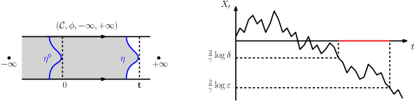
Figure 5: Illustration of the proof of Proposition 6.13. On the left $(\phi,\mathbf{t},\eta^{0})$ is sampled from $M\times dt\times\mathcal{L}^{\alpha}_{\kappa}$ and $\eta=\eta^{0}+\mathbf{t}$. The curve $\eta^{0}$ satisfies $\sup_{z\in\eta_{0}}\operatorname{Re}z=0$ and the field $\phi$ satisfies $\mu_{\phi}(\{z\in\mathcal{C}:\operatorname{Re}z\leq 0\})=1$. The domain $D^{-}_{\eta}$ is colored grey. The event $E^{\prime}_{\delta,\varepsilon}$ is $\{\ell_{\phi}(\eta)\in(\varepsilon,\delta)\textrm{ and }\mu_{\phi}(D_{\eta}^{-})>1\}$. If $E^{\prime}_{\delta,\varepsilon}$ occurs, we have $\ell_{\phi}(\eta)\approx e^{\frac{\gamma}{2}X_{\bf t}}$. Therefore $\mathbf{t}$ is in an interval close to the red one on the right figure, which is approxiately $(\frac{2}{\gamma(Q-\alpha)}\log\delta^{-1},\frac{2}{\gamma(Q-\alpha)}\log\varepsilon^{-1})$. The proofs of Lemmas 6.17 and 6.19 are done by quantifying this statement in two directions.

The high level idea for proving Proposition 6.13 is the following. Suppose $(\phi,\mathbf{t},\eta^{0})$ is sampled from $M\times dt\times\mathcal{L}_{\kappa}^{\alpha}$. For $s\geq 0$, let $X_{s}$ be the average of $\phi$ on $[s,s+2\pi i]/{\sim}$. For most realizations of $(\phi,\eta^{0})$, the occurrence of $E^{\prime}_{\delta,\varepsilon}$ is equivalent to the event that $\mathbf{t}$ lies in some interval of length $(1+o_{\delta,\varepsilon}(1))\frac{2\log\varepsilon^{-1}}{\gamma(Q-\alpha)}$ determined by $X$. (See Figure 5.) Hence the mass of $E^{\prime}_{\delta,\varepsilon}$ is this length times $|M||\mathcal{L}_{\kappa}^{\alpha}|$. In the rest of this section, we first prove a few properties for $X$ in Section 6.2.1 and then prove Proposition 6.13 in Section 6.2.2.

6.2.1 The field average process

We need the following description of the law of $\phi|_{\mathcal{C}_{+}}$ and $(X_{s})_{s\geq 0}$, where $\mathcal{C}_{+}:=\{z\in\mathcal{C}\>:\>\operatorname{Re}z>0\}$ is the right half cylinder.

Lemma 6.14.

Let $\phi$ be a sample from $M$. Conditioned on $\phi|_{\mathcal{C}_{-}}$, the conditional law of $\phi|_{\mathcal{C}_{+}}$ is the law of $\phi_{0}+\hat{\mathfrak{h}}-(Q-\alpha)\operatorname{Re}(\cdot)$, where $\phi_{0}$ is a zero boundary GFF on $\mathcal{C}_{+}$, and $\hat{\mathfrak{h}}$ is a harmonic function determined by $\phi|_{\mathcal{C}_{-}}$ whose average on the circle $[s,s+2\pi i]/{\sim}$ does not depend on $s$. Moreover, let $X_{s}$ be the average of $\phi$ on $[s,s+2\pi i]/{\sim}$. Conditioned on $X_{0}$, the conditional law of $(X_{s}-X_{0})_{s\geq 0}$ is the law of $(B_{s}-(Q-\alpha)s)_{s\geq 0}$ where $B_{s}$ is a Brownian motion.

Proof.

The first statement is the sphere analog of [AG21, Lemmas 2.10 and 2.11] based on the domain Markov property of Gaussian free field. The proof is identical so we omit it. The second statement on $(X_{s})_{s\geq 0}$ follows from the first statement. ∎

Proposition 6.13 essentially follows from the fact that the field average process $(X_{s})_{s\geq 0}$ looks like a line of slope $-(Q-\alpha)$. We now introduce two random times to quantify this. For $y>0$, let

$$\sigma_{y}=\inf\{s>0\>:\>X_{s}<\frac{2}{\gamma}\log y\}\quad\textrm{and}\quad\tau_{y}=\sup\{s>0\>:\>X_{s}>\frac{2}{\gamma}\log y\}.$$ (6.13)

Lemma 6.15.

$M$-a.e. the field $\phi$ satisfies $\lim_{y\to 0}\frac{\sigma_{y}}{\log y^{-1}}=\lim_{y\to 0}\frac{\tau_{y}}{\log y^{-1}}=\frac{2}{\gamma(Q-\alpha)}$.

Proof.

Given Lemma 6.14, this is a straightforward fact about drifted Brownian motion. ∎

The proof of the upper bound in Proposition 6.13 will rely on the following lemma.

Lemma 6.16.

Sample $(\phi,\mathbf{t},\eta^{0})$ from $M\times dt\times\mathcal{L}_{\kappa}^{\alpha}$ and set $\eta=\eta^{0}+\mathbf{t}$. Let $\mathfrak{l}=\ell_{\phi}(\eta)$, which is the boundary length of the quantum surface $(D_{\eta}^{-},\phi)/{\sim_{\gamma}}$. Fix $\zeta\in(0,1)$. Then there exists a constant $C>0$ and a function $\mathrm{err}(\ell)$ such that $\lim_{\ell\downarrow 0}\mathrm{err}(\ell)=0$, and conditioned on $(D_{\eta}^{-},\phi)/{\sim_{\gamma}}$, the conditional probability of $\{\mathbf{t}\in(\sigma_{{\mathfrak{l}}^{1-\zeta}}-C,\tau_{{\mathfrak{l}}^{1+\zeta}})\}$ is at least $1-\mathrm{err}(\mathfrak{l})$.

Proof.

We first introduce $C$ and $\mathrm{err},$ and then show that they satisfy Lemma 6.16. Recall that $\eta^{0}$ is a loop in $\mathcal{C}$ separating $\pm\infty$ and with $\sup_{z\in\eta^{0}}\operatorname{Re}z=0$. Let $D_{\eta^{0}}^{+}$ be the connected component of $\mathcal{C}\backslash\eta^{0}$ containing $+\infty$. Let $f:\mathcal{C}_{+}\to D_{\eta^{0}}^{+}$ be the unique conformal map such that $f(+\infty)=+\infty$ and $\lim_{z\to+\infty}(f(z)-z)\in\mathbbm{R}$. By standard conformal distortion estimates (e.g. [MS19, Lemma 2.4]), for $C=e^{10}$ we have

$$|f(z)-z|<\frac{C}{3}\quad\textrm{and}\quad|f^{\prime\prime}(z)|<\frac{1}{2}<|f^{\prime}(z)|<2\quad\textrm{for }\operatorname{Re}z>\frac{C}{3}.$$ (6.14)

Let $g$ be a fixed smooth function on $\mathcal{C}$ supported on $\{\operatorname{Re}z\in(C-1,C)\}$ such that $\int g(z)\,dz=1$ and $g$ is invariant under rotations against the axis of $\mathcal{C}$. Let $S$ be the collection of smooth functions $\xi$ that are supported on $\{\operatorname{Re}z\in[\frac{2}{3}C-1,\frac{4}{3}C]\}\subset\mathcal{C}_{+}$ and satisfy $\|\xi\|_{\infty}\leq 4\|g\|_{\infty}$ and $\|\nabla\xi\|_{\infty}\leq 8(\|g\|_{\infty}+\|\nabla g\|_{\infty})$. Let

$$\mathrm{err}(\ell):=\mathcal{M}_{1}^{\mathrm{disk}}(\alpha;1)^{\#}\Big{[}\sup_{\xi\in S}|(h,\xi)|+Q\log 2\geq-\frac{2\zeta}{\gamma}\log\ell\Big{]}$$ (6.15)

where $(\mathcal{C}_{+},h,+\infty)$ is an embedding of a sample from $\mathcal{M}_{1}^{\mathrm{disk}}(\alpha;1)^{\#}$, the probablity measure proportional to $\mathcal{M}_{1}^{\mathrm{disk}}(\alpha;1)$. Since the space $S$ is invariant under rotations against the axis of $\mathcal{C}$, the probability in (6.15) does not depend on the choice of the embedding. Moreover, since $h$ is a.s. in the Sobolev space of index $-1$, we see that $\sup_{\xi\in S}|(h,\xi)|<\infty$ a.s. hence $\lim_{\ell\to 0}\mathrm{err}(\ell)=0$.

We now show that $C$ and $\mathrm{err}$ satisfy Lemma 6.16. Set $\phi^{0}(\cdot)=\phi(\cdot+\mathbf{t})$ and $\hat{\phi}=\phi^{0}\circ f+Q\log|f^{\prime}|-\frac{2}{\gamma}\log\mathfrak{l}$. Then $(D_{\eta}^{+},\phi,+\infty)/{\sim_{\gamma}}=(D_{\eta_{0}}^{+},\phi^{0},+\infty)/{\sim_{\gamma}}$ hence $(\mathcal{C}_{+},\hat{\phi},+\infty)/{\sim_{\gamma}}=(D_{\eta}^{+},\phi-\frac{2}{\gamma}\log\mathfrak{l},+\infty)/{\sim_{\gamma}}$. Moreover,

$$(\phi^{0},g)-\frac{2}{\gamma}\log\mathfrak{l}=(\hat{\phi}\circ f^{-1}+Q\log|(f^{-1})^{\prime}|,g)=(\hat{\phi},|f^{\prime}|^{2}g\circ f)+(Q\log|(f^{-1})^{\prime}|,g).$$ (6.16)

By (6.14) and the definition of $S$, we have $|f^{\prime}|^{2}g\circ f\in S$. Then by (6.14) and (6.16), we have

$$\big{|}(\phi^{0},g)-\frac{2}{\gamma}\log\mathfrak{l}\big{|}\leq|(\hat{\phi},|f^{\prime}|^{2}g\circ f)|+|(Q\log|(f^{-1})^{\prime}|,g)|\leq\sup_{\xi\in S}|(\hat{\phi},\xi)|+Q\log 2.$$

Recall from the proof of Lemma 6.11 that the law of $(\mathcal{C},\phi,\eta,+\infty,-\infty)/{\sim_{\gamma}}$ is the restriction of $\mathcal{M}_{2}^{\mathrm{sph}}(\alpha)\otimes\operatorname{SLE}_{\kappa}^{\mathrm{sep},\alpha}$ to the event that the total quantum area is larger than $1$. By Proposition 6.2, conditioning on $(D_{\eta}^{-},\phi)/{\sim_{\gamma}}$, the conditional law of $(D_{\eta}^{+},\phi,+\infty)/{\sim_{\gamma}}$ is $\mathcal{M}_{1}^{\mathrm{disk}}(\alpha;\mathfrak{l})^{\#}$, hence the conditional law of $(\mathcal{C}_{+},\hat{\phi},+\infty)/{\sim_{\gamma}}$ is $\mathcal{M}_{1}^{\mathrm{disk}}(\alpha;1)^{\#}$. Therefore, by (6.15) and (6.16), conditioning on $(D_{\eta}^{-},\phi)/{\sim_{\gamma}}$, the conditional probability of the event $\mathopen{}\mathclose{{}\left|(\phi^{0},g)-\frac{2}{\gamma}\log\mathfrak{l}}\right|<-\frac{2\zeta}{\gamma}\log\mathfrak{l}$ is at least $1-\mathrm{err}(\mathfrak{l})$. Since $g$ is supported on $\{\operatorname{Re}z\in(C-1,C)\}$, if $\mathopen{}\mathclose{{}\left|(\phi^{0},g)-\frac{2}{\gamma}\log\mathfrak{l}}\right|<-\frac{2\zeta}{\gamma}\log\mathfrak{l}$, then there exists $s\in[C-1,C]$ such that the average of $\phi^{0}$ on $[s,s+2\pi i]$ lies in $((1+\zeta)\frac{2}{\gamma}\log\mathfrak{l},(1-\zeta)\frac{2}{\gamma}\log\mathfrak{l})$. This gives $X_{\mathbf{t}+s}\in((1+\zeta)\frac{2}{\gamma}\log\mathfrak{l},(1-\zeta)\frac{2}{\gamma}\log\mathfrak{l})$ hence $\mathbf{t}+s\in(\sigma_{{\mathfrak{l}}^{1-\zeta}},\tau_{{\mathfrak{l}}^{1+\zeta}})$ for some $s\in[C-1,C]$. Therefore $\mathbf{t}\in(\sigma_{{\mathfrak{l}}^{1-\zeta}}-C,\tau_{{\mathfrak{l}}^{1+\zeta}})$, which gives Lemma 6.16 with our choice of $C$ and $\mathrm{err}$. ∎

6.2.2 Proof of Proposition 6.13

We refer to Figure 5 and the paragraph above Section 6.2.1 for an illustration of our proof ideas. We will write $o_{\delta,\varepsilon}(1)$ as an error term satisfying $\lim_{\delta\to 0}\limsup_{\varepsilon\to 0}|o_{\delta,\varepsilon}(1)|=0$ which can change from place to place. We first prove the lower bound for $(M\times dt\times\mathcal{L}_{\kappa}^{\alpha})[E^{\prime}_{\delta,\varepsilon}]$.

Lemma 6.17.

We have $(M\times dt\times\mathcal{L}_{\kappa}^{\alpha})[E^{\prime}_{\delta,\varepsilon}]\geq(1+o_{\delta,\varepsilon}(1))|M||\mathcal{L}_{\kappa}^{\alpha}|\frac{2\log\varepsilon^{-1}}{\gamma(Q-\alpha)}.$

We will prove Lemma 6.17 by a coupling of the probability measure $M^{\#}=M/|M|$ and cylindrical GFF measure $P_{\mathcal{C}}$. Recall that for a sample $h$ from $P_{\mathcal{C}}$, it can be written as $h=h_{1}+h_{2}$, where $h_{1}$ is constant on vertical circles and $h_{2}$ is the lateral component that has mean zero on all such circles.

Lemma 6.18.

There exists a coupling of $h$ sampled from $P_{\mathcal{C}}$ and $\phi$ sampled from $M^{\#}$ such that $h_{2}$ is independent of $(X_{s})_{s\geq 0}$, and moreover, $\sup_{\operatorname{Re}z>1}|{\mathfrak{h}}(z)|<\infty$ where $\mathfrak{h}(z)=\phi(z)-h_{2}(z)-X_{\operatorname{Re}z}$.

Proof.

By [MS17, Proposition 2.8], on $\mathcal{C}_{+}$ the field $h$ can be written as $h_{0}+\tilde{\mathfrak{h}}$ where $h_{0}$ is a zero boundary GFF on $\mathcal{C}_{+}$ and $\tilde{\mathfrak{h}}$ is an independent harmonic function on $\mathcal{C}_{+}$ such that $\sup_{\operatorname{Re}z>1}|\tilde{\mathfrak{h}}(z)|<\infty$. Similarly, by Lemma 6.14, $\phi(z)+(Q-\alpha)\operatorname{Re}z$ on $\mathcal{C}_{+}$ can be written as $\phi_{0}+\hat{\mathfrak{h}}$ with the same properties. Coupling $h$ and $\phi$ such that $h_{0}=\phi_{0}$ and $\tilde{\mathfrak{h}}$ is independent of $\phi$, we are done. ∎

Proof of Lemma 6.17.

Let $\mathbbm{P}$ be the probability measure corresponding to the law of $(\phi,h)$ as coupled in Lemma 6.18. Let $(\phi,h,\mathbf{t},\eta^{0})$ be a sample from $\mathbbm{P}\times dt\times\mathcal{L}_{\kappa}^{\alpha}$. Then the law of $(\phi,\mathbf{t},\eta^{0})$ is $M^{\#}\times dt\times\mathcal{L}_{\kappa}^{\alpha}$, where $M^{\#}=M/|M|$. Let $h_{2}$ and $\mathfrak{h}$ be defined as in Lemma 6.18 so that $\phi=h_{2}+X_{\operatorname{Re}\cdot}+\mathfrak{h}$. Fix $\zeta\in(0,0.1)$ which will be sent to zero later. Let $I_{\delta,\varepsilon}$ be the interval $((1+3\zeta)\frac{2}{\gamma(Q-\alpha)}\log\delta^{-1}+\delta^{-1},(1-3\zeta)\frac{2}{\gamma(Q-\alpha)}\log\varepsilon^{-1})$. Let

$$G_{\delta,\varepsilon}:=\{I_{\delta,\varepsilon}\subset(\tau_{\delta^{1+2\zeta}}+\delta^{-1},\sigma_{\varepsilon^{1-2\zeta}})\quad\textrm{and}\quad\sup_{\operatorname{Re}z>1}|{\mathfrak{h}}(z)|<\zeta\cdot\frac{2}{\gamma}\log\delta^{-1}\},$$

where the random times $\sigma_{y},\tau_{y}$ are as in (6.13). By Lemma 6.15 we have $\mathbbm{P}[I_{\delta,\varepsilon}\subset(\tau_{\delta^{1+2\zeta}}+\delta^{-1},\sigma_{\varepsilon^{1-2\zeta}})]=1-o_{\delta,\varepsilon}(1)$. Since $\sup_{\operatorname{Re}z>1}|{\mathfrak{h}}(z)|<\infty$ almost surely, we have $\mathbbm{P}[G_{\delta,\varepsilon}]=1-o_{\delta,\varepsilon}(1)$.

Fix $n>0$. Let $A_{n}=\{\inf_{z\in\eta^{0}}\operatorname{Re}z>-n\}$. Then $\mathcal{L}^{\alpha}_{\kappa}[A_{n}]<\infty$. Let $\eta=\eta^{0}+\mathbf{t}$ and $\ell_{h_{2}}(\eta)$ be the quantum length of $\eta$ with respect to $h_{2}$. Define the event

$$E^{\prime}_{\delta,\varepsilon}(n):=\{A_{n}\textrm{ occurs},\quad\mathbf{t}\in I_{\delta,\varepsilon},\quad\textrm{and}\quad\ell_{h_{2}}(\eta)\in(\varepsilon^{\zeta},\delta^{-\zeta})\}.$$

Suppose $n<\delta^{-1}<\frac{2\zeta}{\gamma(Q-\alpha)}\log\varepsilon^{-1}$ and the event $E^{\prime}_{\delta,\varepsilon}(n)\cap G_{\delta,\varepsilon}$ occurs. Since $\mathbf{t}\in I_{\delta,\varepsilon}$ and $G_{\delta,\varepsilon}\cap A_{n}$ occurs, we have $\operatorname{Re}z\in(\tau_{\delta^{1+2\zeta}},\sigma_{\varepsilon^{1-2\zeta}})$ for each $z\in\eta$, hence $\mathcal{C}_{-}:=\{z\in\mathcal{C}:\operatorname{Re}z\leq 0\}\subset D^{-}_{\eta}$. By the definition of $\phi$ we have $\mu_{\phi}(D_{\eta}^{-})\geq\mu_{\phi}(\mathcal{C}_{-})\geq 1$. Moreover, from the bound on $\sup_{\operatorname{Re}z>1}|{\mathfrak{h}}(z)|$ we have $\frac{\gamma}{2}(X_{\operatorname{Re}z}+\mathfrak{h}(z))\in((1-\zeta)\log\varepsilon,(1+\zeta)\log\delta)$ for each $z\in\eta$. Now $\ell_{h_{2}}(\eta)\in(\varepsilon^{\zeta},\delta^{-\zeta})$ yields $\ell_{\phi}(\eta)\in(\varepsilon,\delta)$. This gives $E^{\prime}_{\delta,\varepsilon}(n)\cap G_{\delta,\varepsilon}\subset E^{\prime}_{\delta,\varepsilon}=\{\mu_{\phi}(D_{\eta}^{-})\geq 1,\ell_{\phi}(\eta)\in(\varepsilon,\delta)\}$. Therefore

$$(\mathbbm{P}\times dt\times\mathcal{L}_{\kappa}^{\alpha})[E^{\prime}_{\delta,\varepsilon}]\geq(\mathbbm{P}\times dt\times\mathcal{L}_{\kappa}^{\alpha})[E^{\prime}_{\delta,\varepsilon}(n)]-(\mathbbm{P}\times dt\times\mathcal{L}_{\kappa}^{\alpha})[E^{\prime}_{\delta,\varepsilon}(n)\setminus G_{\delta,\varepsilon}].$$ (6.17)

We claim that

$$(\mathbbm{P}\times dt\times\mathcal{L}_{\kappa}^{\alpha})[E^{\prime}_{\delta,\varepsilon}(n)]=(1-o_{\delta,\varepsilon}(1))|I_{\delta,\varepsilon}|\mathcal{L}^{\alpha}_{\kappa}[A_{n}]\textrm{ and }(\mathbbm{P}\times dt\times\mathcal{L}_{\kappa}^{\alpha})[E^{\prime}_{\delta,\varepsilon}(n)\setminus G_{\delta,\varepsilon}]=o_{\delta,\varepsilon}(1)|I_{\delta,\varepsilon}|.$$ (6.18)

Since the law of $h_{2}$ is translation invariant, namely $h_{2}\stackrel{{\scriptstyle d}}{{=}}h_{2}(\cdot-t)$ for each $t\in\mathbbm{R}$, we have

$$(\mathbbm{P}\times dt\times\mathcal{L}_{\kappa}^{\alpha})[E^{\prime}_{\delta,\varepsilon}(n)]=|I_{\delta,\varepsilon}|(\mathbbm{P}\times\mathcal{L}^{\alpha}_{\kappa})[\ell_{h_{2}}(\eta^{0})\in(\varepsilon^{\zeta},\delta^{-\zeta}),A_{n}]$$

$$=|I_{\delta,\varepsilon}|(\mathbbm{P}\times\mathcal{L}^{\alpha}_{\kappa})[A_{n}]-|I_{\delta,\varepsilon}|(\mathbbm{P}\times\mathcal{L}^{\alpha}_{\kappa})[\ell_{h_{2}}(\eta^{0})\notin(\varepsilon^{\zeta},\delta^{-\zeta}),A_{n}]=(1-o_{\delta,\varepsilon}(1))|I_{\delta,\varepsilon}|\mathcal{L}^{\alpha}_{\kappa}[A_{n}].$$

In the last line we used $(\mathbbm{P}\times\mathcal{L}^{\alpha}_{\kappa})[A_{n}]=\mathcal{L}^{\alpha}_{\kappa}[A_{n}]<\infty$ and $(\mathbbm{P}\times\mathcal{L}^{\alpha}_{\kappa})[\ell_{h_{2}}(\eta^{0})\notin(\varepsilon^{\zeta},\delta^{-\zeta})|A_{n}]=o_{\delta,\varepsilon}(1)$, the latter of which holds because $\ell_{h_{2}}(\eta^{0})<\infty$ a.e.  in $\mathbbm{P}\times\mathcal{L}^{\alpha}_{\kappa}$. This gives the first identity in (6.18).

The second identity in (6.18) is proved by as follows:

$$(\mathbbm{P}\times dt\times\mathcal{L}_{\kappa}^{\alpha})[E^{\prime}_{\delta,\varepsilon}(n)\setminus G_{\delta,\varepsilon}]\leq(\mathbbm{P}\times dt\times\mathcal{L}_{\kappa}^{\alpha})[A_{n}\setminus G_{\delta,\varepsilon}\textrm{ and }\mathbf{t}\in I_{\delta,\varepsilon}]$$

$$=\mathbbm{P}[G_{\delta,\varepsilon}\textrm{ does not occur}]\times|I_{\delta,\varepsilon}|\times\mathcal{L}^{\alpha}_{\kappa}[A_{n}]=o_{\delta,\varepsilon}(1)|I_{\delta,\varepsilon}|\mathcal{L}^{\alpha}_{\kappa}[A_{n}].$$

By (6.17) and (6.18), for a fixed $n$, we have $(\mathbbm{P}\times dt\times\mathcal{L}_{\kappa}^{\alpha})[E^{\prime}_{\delta,\varepsilon}]\geq(1-o_{\delta,\varepsilon}(1))|I_{\delta,\varepsilon}||\mathcal{L}^{\alpha}_{\kappa}[A_{n}]$ hence

$$\frac{1}{|M|}(M\times dt\times\mathcal{L}_{\kappa}^{\alpha})[E^{\prime}_{\delta,\varepsilon}]\geq(1-o_{\delta,\varepsilon}(1))|I_{\delta,\varepsilon}|\mathcal{L}^{\alpha}_{\kappa}[A_{n}]\geq(1-o_{\delta,\varepsilon}(1))\mathcal{L}^{\alpha}_{\kappa}[A_{n}](1-4\zeta)\frac{2\log\varepsilon^{-1}}{\gamma(Q-\alpha)}.$$

Sending $\varepsilon\to 0$, $\delta\to 0$, and $\zeta\to 0$ in order, we see that

$$\lim_{\delta\to 0}\liminf_{\varepsilon\to 0}\frac{(M\times dt\times\mathcal{L}_{\kappa}^{\alpha})[E^{\prime}_{\delta,\varepsilon}]\times\gamma(Q-\alpha)}{2\log\varepsilon^{-1}}\geq|M|\mathcal{L}^{\alpha}_{\kappa}[A_{n}].$$

Since $\mathcal{L}^{\alpha}_{\kappa}[A_{n}]\rightarrow|\mathcal{L}^{\alpha}_{\kappa}|$, sending $n\to\infty$ we conclude the proof. ∎

It remains to prove the upper bound for $(M\times dt\times\mathcal{L}_{\kappa}^{\alpha})[E^{\prime}_{\delta,\varepsilon}]$.

Lemma 6.19.

We have $(M\times dt\times\mathcal{L}_{\kappa}^{\alpha})[E^{\prime}_{\delta,\varepsilon}]\leq(1+o_{\delta,\varepsilon}(1))|M||\mathcal{L}_{\kappa}^{\alpha}|\frac{2\log\varepsilon^{-1}}{\gamma(Q-\alpha)}.$

Proof.

Recall $\sigma$ and $\tau$ defined in (6.13). For $C>0$, consider the event

$$F_{x,y,C}=\{(\phi,\mathbf{t},\eta^{0})\>:\>\mathbf{t}\in(\sigma_{x}-C,\tau_{y})\}.$$ (6.19)

We will prove Lemma 6.19 by first bounding $(M\times dt\times\mathcal{L}_{\kappa}^{\alpha})[F_{x,y,C}]$ and then comparing $E^{\prime}_{\delta,\varepsilon}$ to $F_{\delta^{1-\zeta},\varepsilon^{1+\zeta},C}$. More precisely, we will prove two estimates. First, for each $x>0$, we have

$$(M\times dt\times\mathcal{L}_{\kappa}^{\alpha})[F_{x,y,C}]\leq(1+o_{y}(1))|M||\mathcal{L}_{\kappa}^{\alpha}|(\frac{2\log y^{-1}}{\gamma(Q-\alpha)}+C)\quad\textrm{as }y\to 0,$$ (6.20)

where $o_{y}(1)\to 0$ uniformly in $C$. Moreover, for a fixed $\zeta\in(0,1)$ there exists some $C>0$ such that

$$(M\times dt\times\mathcal{L}_{\kappa}^{\alpha})[F_{\delta^{1-\zeta},\varepsilon^{1+\zeta},C}\mid E^{\prime}_{\delta,\varepsilon}]=1-o_{\delta,\varepsilon}(1).$$ (6.21)

Given (6.20) and (6.21), we see that for any fixed $\zeta>0$ there exists some $C>0$ such that

$$(M\times dt\times\mathcal{L}_{\kappa}^{\alpha})[E^{\prime}_{\delta,\varepsilon}]\leq(1+o_{\delta,\varepsilon}(1))(M\times dt\times\mathcal{L}_{\kappa}^{\alpha})[F_{\delta^{1-\zeta},\varepsilon^{1+\zeta},C}]\leq(1+o_{\delta,\varepsilon}(1))|M||\mathcal{L}_{\kappa}^{\alpha}|\frac{(1+\zeta)2\log\varepsilon^{-1}}{\gamma(Q-\alpha)},$$

Sending $\zeta\to 0$ we will get Lemma 6.19.

We first prove (6.20). Note that $(M\times dt\times\mathcal{L}_{\kappa}^{\alpha})[F_{x,y,C}]=M^{\#}[\tau_{y}-\sigma_{x}+C]|M||\mathcal{L}^{\alpha}_{\kappa}|$ from the definition of $F_{x,y,C}$. Hence (6.20) is equivalent to $M^{\#}[\tau_{y}-\sigma_{x}]\leq(1+o_{y}(1))\frac{2\log y^{-1}}{\gamma(Q-\alpha)}$. By Lemma 6.14, the process $X_{s}$ evolves as Brownian motion with drift $-(Q-\alpha)$. Let $T=\inf\{s\geq 0:B^{x}_{s}-(Q-\alpha)s=\frac{2}{\gamma}\log y\}$ where $(B^{x}_{s})_{s\geq 0}$ is a Brownian motion starting from $\frac{2}{\gamma}\log x$. Then $M^{\#}[\tau_{y}-\sigma_{x}]\leq\mathbbm{E}[T]$. Since $\mathbbm{E}[T]=(1+o_{y}(1))\frac{2\log y^{-1}}{\gamma(Q-\alpha)}$, we get (6.20).

Since the event $E^{\prime}_{\delta,\varepsilon}$ is determined by $(D_{\eta}^{-},\phi)/{\sim_{\gamma}}$, and $\ell_{\phi}(\eta)\in(\varepsilon,\delta)$ on $E^{\prime}_{\delta,\varepsilon}$, Lemma 6.16 yields (6.21) with the constant $C$ from Lemma 6.16. This concludes the proof. ∎

Appendix A Continuity of $\operatorname{CLE}_{\kappa}$ as $\kappa\uparrow 4$

In this appendix we supply the continuity in $\kappa$ needed to extend Theorems 1.2 and 1.3 from $\kappa<4$ to $\kappa=4$. We start with a monotonicity statement for $\operatorname{CLE}_{\kappa}$ proved in [SW12].

Lemma A.1 ([SW12]).

There exists a coupling of $\operatorname{CLE}_{\kappa}$ on the unit disk $\mathbbm{D}$ for $\kappa\in(\frac{8}{3},4]$ such that a.s.  each outermost loop of $\operatorname{CLE}_{\kappa_{1}}$ is surrounded by an outermost loop of $\operatorname{CLE}_{\kappa_{2}}$ if $\kappa_{1}<\kappa_{2}\leq 4$.

Proof.

By [SW12, Theorems 1.5, 1.6], the law of the boundaries of outermost loop clusters in a Brownian loop soup with intensity $c_{\kappa}=(3\kappa-8)(6-\kappa)/2\kappa$ is given by the outermost loops of $\operatorname{CLE}_{\kappa}$. Now the monotonicity of $c_{\kappa}$ in $\kappa\in(\frac{8}{3},4]$ yields the desired monotonicity in Lemma A.1. ∎

We recall the formula from [SSW09] for the conformal radii of CLE.

Theorem A.2 ([SSW09]).

For $\kappa\in(8/3,8)$, let $\eta_{\kappa}$ be the outermost loop surrounding $0$ of a $\operatorname{CLE}_{\kappa}$ on $\mathbbm{D}$. Let $\mathrm{CR}(\eta_{\kappa},0)$ be the conformal radius of the region surrounded by $\eta_{\kappa}$ viewed from 0. Then

$$\mathbbm{E}[\mathrm{CR}(\eta_{\kappa},0)^{\lambda}]=\frac{-\cos(\frac{4\pi}{\kappa})}{\cos\mathopen{}\mathclose{{}\left(\pi\sqrt{(1-\frac{4}{\kappa})^{2}-\frac{8\lambda}{\kappa}}}\right)}\quad\textrm{for }\lambda>\frac{3\kappa}{32}+\frac{2}{\kappa}-1.$$

Recall that the Hausdorff distance between two closed sets $E_{1},E_{2}$ on a metric space $(X,d)$ is given by $\max\{\sup_{x\in E_{1}}\{d(x,E_{2})\},\sup_{x\in E_{2}}\{d(x,E_{1})\}\}$. Lemma A.1 and Theorem A.2 yield the following continuity result.

Lemma A.3.

Suppose we are in the coupling in Lemma A.1. For each $z\in\mathbbm{D}$, let $\eta_{\kappa}(z)$ be the outermost loop around $z$ of the $\operatorname{CLE}_{\kappa}$. For any fixed $z$, viewed as closed sets, $\eta_{\kappa}(z)$ converges almost surely to $\eta_{4}(z)$ in the Hausdorff metric as $\kappa\uparrow 4$.

Proof.

By the conformal invariance of $\operatorname{CLE}_{\kappa}$ we assume $z=0$ because the same argument will work for a general $z$. In this case we simply write $\eta_{\kappa}(0)$ as $\eta_{\kappa}$. Since $\eta_{\kappa_{1}}$ is surrounded by $\eta_{\kappa_{2}}$ if $\kappa_{1}<\kappa_{2}\leq 4$. we see that $\mathrm{CR}(\eta_{\kappa},0)$ is increasing in $\kappa$. By the explicit formula in Theorem A.2, we have $\lim_{\kappa\uparrow 4}\mathbbm{E}[\mathrm{CR}(\eta_{\kappa},0)]=\mathbbm{E}[\mathrm{CR}(\eta_{\kappa},0)]$. Thus we must have $\lim_{\kappa\uparrow 4}\mathrm{CR}(\eta_{\kappa},0)=\mathrm{CR}(\eta_{4},0)$ a.s.

Let $D_{\kappa}$ be the region surrounded by $\eta_{\kappa}$ and $D_{4^{-}}=\cup_{\kappa<4}D_{\kappa}$. The conformal radius of $D_{4^{-}}$ must be between $\lim_{\kappa\uparrow 4}\mathrm{CR}(\eta_{\kappa},0)$ and $\mathrm{CR}(\eta_{4},0)$, hence equals $\mathrm{CR}(\eta_{4},0)$ a.s. This means that $D_{\kappa}\uparrow D_{4}$ a.s. hence $\eta_{\kappa}\to\eta_{4}$ a.s. in the Hausdorff metric in the coupling in Lemma A.1. ∎

We now prove the continuity of the shape measure $\mathcal{L}_{\kappa}$ of the SLE loop in Theorem 1.3.

Lemma A.4.

We have $\lim_{\kappa\uparrow 4}\mathcal{L}_{\kappa}=\mathcal{L}_{4}$ weakly with respect to the Hausdorff metric.

Proof.

We only explain that under the natural parameterization, chordal $\operatorname{SLE}_{\kappa}$ converges to $\operatorname{SLE}_{4}$ as $\kappa\uparrow 4$. Once this is done we get that the two-sided whole plane $\operatorname{SLE}_{\kappa}$ curve $\operatorname{SLE}_{\kappa}^{p\rightleftharpoons q}$ converges to $\operatorname{SLE}_{4}^{p\rightleftharpoons q}$ under natural parametrization as well, since the two-sided curve is characterized by its re-sampling property: conditioned on one of the curve segments between $p$ and $q$, the conditional law of the other is a chordal $\operatorname{SLE}_{\kappa}$ in the complementary domain. From this and the definition of $\operatorname{SLE}_{\kappa}^{\mathrm{loop}}$ we reviewed in Section 2.4, we get the convergence of $\mathcal{L}_{\kappa}$.

We now show that the law of chordal $\operatorname{SLE}_{\kappa}$ on $\mathbbm{H}$ from $0$ to $\infty$ under natural parametrization is continuous as $\kappa\uparrow 4$. We first recall that this family of measures is tight in the local uniform topology of parametrized curves thanks to their Hölder regularity established by Zhan [Zha19]. On the other hand the natural parametrization of $\operatorname{SLE}_{\kappa}$ is characterized by a conformal invariance and domain Markov property considered by Lawler and Sheffield [LS11]. Therefore all subsequential limits of the chordal $\operatorname{SLE}_{\kappa}$ measure agree with $\operatorname{SLE}_{4}$. ∎

Lemma A.5.

Suppose Theorem 1.2 holds for $\kappa\in(8/3,4)$. Then it holds for $\kappa=4$ as well.

Proof.

The right hand side of (1.3) is continuous as $\kappa\uparrow 4$. Therefore $\{\mathrm{CR}(z_{i},\eta_{i})\}_{1\leq i\leq 3}$ for $\kappa<4$ converges in law as $\kappa\uparrow 4$ and the moment generating function of the limit is given by ${C^{\operatorname{CLE}}_{\kappa}(\lambda_{1},\lambda_{2},\lambda_{3})}$ with $\kappa=4$. It remains to show that the limit is given by $\{\mathrm{CR}(z_{i},\eta_{i})\}_{1\leq i\leq 3}$ with $\kappa=4$.

Fix a small $\varepsilon>0$. Let $S$ be the set of simple loops in $\widehat{\mathbbm{C}}$ separating $z_{1}$ from $\{z_{2},z_{3}\}$. Let $S_{\varepsilon}=\{\eta\in S:\mathrm{CR}(z_{1},\eta)>\varepsilon\}$. For $\eta\in S$, let $D_{\eta}$ be the connected component of $\widehat{\mathbbm{C}}\backslash\eta$ containing $z_{2},z_{3}$. For $\kappa\in(8/3,4]$, the law of $(\eta_{1},\Gamma)$ restricted to the event $\eta_{1}\in S_{\varepsilon}$ is the same as that of $(\eta,\Gamma)$ under $1_{\eta=\eta_{1}}\mathrm{Count}_{S_{\varepsilon}\cap\Gamma}(d\eta)\operatorname{CLE}_{\kappa}(d\Gamma)$, where $\mathrm{Count}_{S_{\varepsilon}\cap\Gamma}(d\eta)$ is the counting measure on $S_{\varepsilon}\cap\Gamma$. Given a sample of $(\eta,\Gamma)$ of $\mathrm{Count}_{S_{\varepsilon}\cap\Gamma}(d\eta)\operatorname{CLE}_{\kappa}(d\Gamma)$, let $\Gamma_{+}$ be the subset of $\Gamma$ in $D_{\eta}$ and $F_{\Gamma_{+}}$ be the event that no loop in $\Gamma_{+}$ surrounds both $z_{2}$ and $z_{3}$. Then the event $\eta=\eta_{1}$ is the same as $F_{\Gamma_{+}}$. By Proposition 3.8, for $\kappa\in(8/3,4]$, the law of $\eta$ under $1_{\eta=\eta_{1}}\mathrm{Count}_{S_{\varepsilon}\cap\Gamma}(d\eta)\operatorname{CLE}_{\kappa}(d\Gamma)$ is $\operatorname{CLE}_{\kappa}^{D_{\eta}}[F_{\Gamma_{+}}]1_{\eta\in S_{\varepsilon}}\cdot\operatorname{SLE}_{\kappa}^{\mathrm{loop}}(d\eta)$, where $\operatorname{CLE}_{\kappa}^{D_{\eta}}$ is the law of a $\operatorname{CLE}_{\kappa}$ in $D_{\eta}$.

By Lemmas A.4 and A.3, as $\kappa\uparrow 4$, the measure $\operatorname{CLE}_{\kappa}^{D_{\eta}}[F_{\Gamma_{+}}]1_{\eta\in S_{\varepsilon}}\cdot\operatorname{SLE}_{\kappa}^{\mathrm{loop}}(d\eta)$ on loops converges weakly with respect to the Hausdorff metric to $\operatorname{CLE}_{4}^{D_{\eta}}[F_{\Gamma_{+}}]1_{\eta\in S_{\varepsilon}}\cdot\operatorname{SLE}_{4}^{\mathrm{loop}}(d\eta)$. Therefore the law of $\eta_{1}$ conditioned on the event $\eta_{1}\in S_{\varepsilon}$ as $\kappa\uparrow 4$ converges weakly to the same law with $\kappa=4$. Since $\lim_{\varepsilon\to 0}\mathbbm{P}[\Gamma\cap S_{\varepsilon}\neq\emptyset]=\lim_{\varepsilon\to 0}\mathbbm{P}[\mathrm{CR}(z_{1},\eta_{1})>\varepsilon]=1$ uniformly for $\kappa\in(\kappa_{0},4]$ for a fixed $\kappa_{0}\in(8/3,4)$, we can remove the restriction $\eta_{1}\in S_{\varepsilon}$ and conclude that as $\kappa\uparrow 4$ the law of $\eta_{1}$ converges weakly to the same law when $\kappa=4$.

The conditional law of $(\eta_{2},\eta_{3})$ given $\eta_{1}$ is the law of the two outermost loops surrounding $z_{2},z_{3}$ under the CLE measure $\operatorname{CLE}_{\kappa}^{D_{\eta_{1}}}$ conditioned on these two loops being distinct. By Lemma A.3, the joint law of $(\eta_{1},\eta_{2},\eta_{3})$ has the desired continuity as $\kappa\uparrow 4$. ∎

Appendix B Identities for the modified Bessel function of the second kind

Proof of Equation (2.7).

We will prove the $c=1$ case; the general case then follows from a change of variables. Recall the integral definition of $K_{\nu}(x)$ in (2.6). Using $1+\cosh t=2(\cosh\frac{t}{2})^{2}$ and the fact that $\cosh$ is even, we can express $\int_{0}^{\infty}\frac{1}{\sqrt{x}}e^{-x}K_{\nu}(x)\,dx$ as

$$\iint_{0}^{\infty}\frac{1}{\sqrt{x}}e^{-x(1+\cosh t)}\cosh(\nu t)\,dx\,dt=\sqrt{\pi}\int_{0}^{\infty}\frac{\cosh(\nu t)}{\sqrt{1+\cosh t}}\,dt=\frac{1}{2}\sqrt{\pi/2}\int_{-\infty}^{\infty}\frac{\cosh(\nu t)}{\cosh(t/2)}\,dt.$$

Since $\int\frac{e^{\nu t}}{\cosh(t/2)}\,dt=\int\frac{e^{-\nu t}}{\cosh(t/2)}\,dt$, we have $\int\frac{\cosh(\nu t)}{\cosh(t/2)}\,dt=\int\frac{e^{\nu t}}{\cosh(t/2)}\,dt$. For a random variable $X$ following the hyperbolic secant distribution $\frac{dx}{\pi\cosh x}$, it is known that $\mathbbm{E}[e^{tX}]=\frac{1}{\cos(\pi t/2)}$ for $|t|<1$; see e.g. [Fis14, Section 1.3]. Therefore $\int_{-\infty}^{\infty}\frac{e^{\nu t}}{\cosh(t/2)}\,dt=\frac{2\pi}{\cos(\pi\nu)}.$ This concludes the proof. ∎

Proof of Equation (2.8).

For $r>0$, using the change of coordinates $s=\sqrt{b}$, we get

$$\int_{0}^{\infty}\frac{1}{\sqrt{b}(1+b)(1+b+br)}\,db=\int_{0}^{\infty}\frac{1}{s(1+s^{2})(1+s^{2}(1+r))}2s\,ds=\int_{-\infty}^{\infty}\frac{1}{(1+s^{2})(1+s^{2}(1+r))}\,ds$$

$$=\frac{1}{r}\int_{-\infty}^{\infty}\frac{1+r}{1+s^{2}(1+r)}-\frac{1}{1+s^{2}}\,ds=\pi\frac{\sqrt{1+r}-1}{r}=\frac{\pi}{\sqrt{1+r}+1}.$$

Therefore, using (2.6) and the identity $1+\cosh t=2(\cosh\frac{t}{2})^{2}$, the integral we must evaluate is

$$\iiint_{0}^{\infty}\frac{1}{\sqrt{b}(b+1)}e^{-x(b+1+b\cosh t)}\cosh(\nu t)\,dt\,db\,dx=\iint_{0}^{\infty}\frac{1}{\sqrt{b}(1+b)(1+b+b\cosh t)}\cosh(\nu t)\,db\,dt$$

$$=\pi\int_{0}^{\infty}\frac{\cosh(\nu t)}{\sqrt{1+\cosh t}+1}\,dt=\frac{\pi}{2}\int_{-\infty}^{\infty}\frac{\cosh(\nu t)}{\sqrt{2}\cosh\frac{t}{2}+1}\,dt=\frac{\pi}{2}\int_{-\infty}^{\infty}\frac{e^{\nu t}}{\sqrt{2}\cosh\frac{t}{2}+1}\,dt.$$

For a random variable $X$ following the Perk’s distribution whose density is $\frac{\sin\lambda}{2\lambda}\frac{dx}{\cosh x+\cos(\lambda)}$ with $\lambda\in[0,\pi)$, it is known that $\mathbbm{E}[e^{itX}]=\frac{\pi\sinh(\lambda t)}{\lambda\sinh(\pi t)}$ for $t\in\mathbbm{R}$; see e.g. [Fis14, Section 2.1]. Taking $\lambda=\frac{\pi}{4}$, we have $\int_{-\infty}^{\infty}\frac{e^{\nu t}}{\sqrt{2}\cosh\frac{t}{2}+1}\,dt=\frac{\pi}{\cos(\pi\nu)\cos(\frac{1}{2}\pi\nu)}.$ This concludes the proof. ∎

References

- [AG21] M. Ang and E. Gwynne. Liouville quantum gravity surfaces with boundary as matings of trees. Annales de l’Institut Henri Poincaré, Probabilités et Statistiques, 57(1):1 – 53, 2021.
- [AHS17] J. Aru, Y. Huang, and X. Sun. Two perspectives of the 2D unit area quantum sphere and their equivalence. Comm. Math. Phys., 356(1):261–283, 2017, 1512.06190. MR3694028
- [AHS20] M. Ang, N. Holden, and X. Sun. Conformal welding of quantum disks. arXiv preprint arXiv:2009.08389, 2020.
- [AHS21] M. Ang, N. Holden, and X. Sun. Integrability of SLE via conformal welding of random surfaces. ArXiv e-prints, Apr 2021, 2104.09477.
- [ALS20] J. Aru, T. Lupu, and A. Sepúlveda. Extremal distance and conformal radius of a CLE_4 loop. arXiv e-prints, page arXiv:2004.13570, April 2020, 2004.13570.
- [ARS21] M. Ang, G. Remy, and X. Sun. FZZ formula of boundary Liouville CFT via conformal welding. ArXiv e-prints, Apr 2021, 2104.09478.
- [BBCK18] J. Bertoin, T. Budd, N. Curien, and I. Kortchemski. Martingales in self-similar growth-fragmentations and their connections with random planar maps. Probab. Theory Related Fields, 172(3-4):663–724, 2018. MR3877545
- [BDE19] T. Bautista, A. Dabholkar, and H. Erbin. Quantum Gravity from Timelike Liouville theory. JHEP, 10:284, 2019, 1905.12689.
- [BH19] S. Benoist and C. Hongler. The scaling limit of critical Ising interfaces is CLE3. Ann. Probab., 47(4):2049–2086, 2019, 1604.06975. MR3980915
- [BPZ84] A. A. Belavin, A. M. Polyakov, and A. B. Zamolodchikov. Infinite Conformal Symmetry in Two-Dimensional Quantum Field Theory. Nucl. Phys., B241:333–380, 1984. [,605(1984)].
- [CCM20] L. Chen, N. Curien, and P. Maillard. The perimeter cascade in critical Boltzmann quadrangulations decorated by an loop model. Ann. Inst. Henri Poincaré D, 7(4):535–584, 2020. MR4182775
- [Cer19] B. Cerclé. Unit boundary length quantum disk: a study of two different perspectives and their equivalence. ArXiv e-prints, Dec 2019, 1912.08012.
- [CN08] F. Camia and C. M. Newman. and from critical percolation. In Probability, geometry and integrable systems, volume 55 of Math. Sci. Res. Inst. Publ., pages 103–130. Cambridge Univ. Press, Cambridge, 2008, math/0611116. MR2407594 (2009h:82032)
- [DDDF20] J. Ding, J. Dubédat, A. Dunlap, and H. Falconet. Tightness of Liouville first passage percolation for . Publ. Math. Inst. Hautes Études Sci., 132:353–403, 2020. MR4179836
- [DKRV16] F. David, A. Kupiainen, R. Rhodes, and V. Vargas. Liouville quantum gravity on the Riemann sphere. Comm. Math. Phys., 342(3):869–907, 2016, 1410.7318. MR3465434
- [DLG02] T. Duquesne and J.-F. Le Gall. Random trees, Lévy processes and spatial branching processes. Astérisque, (281):vi+147, 2002. MR1954248
- [DLMF] NIST Digital Library of Mathematical Functions. http://dlmf.nist.gov/, Release 1.1.0 of 2020-12-15. F. W. J. Olver, A. B. Olde Daalhuis, D. W. Lozier, B. I. Schneider, R. F. Boisvert, C. W. Clark, B. R. Miller, B. V. Saunders, H. S. Cohl, and M. A. McClain, eds.
- [DMS14] B. Duplantier, J. Miller, and S. Sheffield. Liouville quantum gravity as a mating of trees. ArXiv e-prints, September 2014, 1409.7055.
- [DO94] H. Dorn and H.-J. Otto. Two- and three-point functions in Liouville theory. Nuclear Physics B, 429:375–388, October 1994, hep-th/9403141.
- [DRV16] F. David, R. Rhodes, and V. Vargas. Liouville quantum gravity on complex tori. J. Math. Phys., 57(2):022302, 25, 2016, 1504.00625. MR3450564
- [DS11] B. Duplantier and S. Sheffield. Liouville quantum gravity and KPZ. Invent. Math., 185(2):333–393, 2011, 1206.0212. MR2819163 (2012f:81251)
- [Dur10] R. Durrett. Probability: theory and examples. Cambridge Series in Statistical and Probabilistic Mathematics. Cambridge University Press, Cambridge, fourth edition, 2010. MR2722836 (2011e:60001)
- [DV11] G. Delfino and J. Viti. On three-point connectivity in two-dimensional percolation. J. Phys. A, 44:032001, 2011, 1009.1314.
- [Fis14] M. J. Fischer. Generalized hyperbolic secant distributions. SpringerBriefs in Statistics. Springer, Heidelberg, 2014. With applications to finance. MR3157090
- [FZZ00] V. Fateev, A. B. Zamolodchikov, and A. B. Zamolodchikov. Boundary Liouville field theory. 1. Boundary state and boundary two point function. 1 2000, hep-th/0001012.
- [GHS19] E. Gwynne, N. Holden, and X. Sun. Mating of trees for random planar maps and Liouville quantum gravity: a survey. ArXiv e-prints, Oct 2019, 1910.04713.
- [GKRV20] C. Guillarmou, A. Kupiainen, R. Rhodes, and V. Vargas. Conformal bootstrap in Liouville Theory. arXiv e-prints, page arXiv:2005.11530, May 2020, 2005.11530.
- [GM21] E. Gwynne and J. Miller. Existence and uniqueness of the Liouville quantum gravity metric for . Invent. Math., 223(1):213–333, 2021. MR4199443
- [GMQ18] E. Gwynne, J. Miller, and W. Qian. Conformal invariance of CLE on the Riemann sphere for . International Math Research Notices, to appear, 2018, 1811.00514.
- [GMS21] E. Gwynne, J. Miller, and S. Sheffield. The Tutte embedding of the mated-CRT map converges to Liouville quantum gravity. The Annals of Probability, 49(4):1677–1717, 2021.
- [GRV19] C. Guillarmou, R. Rhodes, and V. Vargas. Polyakov’s formulation of bosonic string theory. Publ. Math. Inst. Hautes Études Sci., 130:111–185, 2019. MR4028515
- [Gwy20] E. Gwynne. Random surfaces and Liouville quantum gravity. Notices Amer. Math. Soc., 67(4):484–491, 2020. MR4186266
- [HJS20] Y. He, J. L. Jacobsen, and H. Saleur. Geometrical four-point functions in the two-dimensional critical -state Potts model: The interchiral conformal bootstrap. JHEP, 12:019, 2020, 2005.07258.
- [HMW11] D. Harlow, J. Maltz, and E. Witten. Analytic Continuation of Liouville Theory. JHEP, 12:071, 2011, 1108.4417.
- [HRV18] Y. Huang, R. Rhodes, and V. Vargas. Liouville quantum gravity on the unit disk. Ann. Inst. Henri Poincaré Probab. Stat., 54(3):1694–1730, 2018, 1502.04343. MR3825895
- [HS19] N. Holden and X. Sun. Convergence of uniform triangulations under the Cardy embedding. ArXiv e-prints, May 2019, 1905.13207.
- [IJS16] Y. Ikhlef, J. L. Jacobsen, and H. Saleur. Three-point functions in liouville theory and conformal loop ensembles. Physical review letters, 116(13):130601, 2016.
- [Kal17] O. Kallenberg. Random measures, theory and applications, volume 77 of Probability Theory and Stochastic Modelling. Springer, Cham, 2017. MR3642325
- [KP07] I. K. Kostov and V. B. Petkova. Non-rational 2-D quantum gravity. I. World sheet CFT. Nucl. Phys. B, 770:273–331, 2007, hep-th/0512346.
- [KPZ88] V. Knizhnik, A. Polyakov, and A. Zamolodchikov. Fractal structure of 2D-quantum gravity. Modern Phys. Lett A, 3(8):819–826, 1988.
- [KRV17] A. Kupiainen, R. Rhodes, and V. Vargas. Integrability of Liouville theory: proof of the DOZZ Formula. Annals of Mathematics, to appear, 2017, 1707.08785.
- [KS07] M. Kontsevich and Y. Suhov. On Malliavin measures, SLE, and CFT. Tr. Mat. Inst. Steklova, 258(Anal. i Osob. Ch. 1):107–153, 2007. MR2400527
- [KS16] A. Kemppainen and S. Smirnov. Conformal invariance in random cluster models II: Full scaling limit as a branching SLE. arXiv preprint arXiv:1609.08527, 2016.
- [KSZ06] P. Kleban, J. J. H. Simmons, and R. M. Ziff. Anchored Critical Percolation Clusters and 2-D Electrostatics. Phys. Rev. Lett., 97:115702, 2006, cond-mat/0605120.
- [KW04] R. Kenyon and D. B. Wilson. Conformal radii of loop models. 2004. Manuscript.
- [KW16] A. Kemppainen and W. Werner. The nested simple conformal loop ensembles in the Riemann sphere. Probab. Theory Related Fields, 165(3-4):835–866, 2016, 1402.2433. MR3520020
- [LJS19] J. Lykke Jacobsen and H. Saleur. Bootstrap approach to geometrical four-point functions in the two-dimensional critical -state Potts model: A study of the -channel spectra. JHEP, 01:084, 2019, 1809.02191.
- [LR15] G. F. Lawler and M. A. Rezaei. Minkowski content and natural parameterization for the Schramm-Loewner evolution. Ann. Probab., 43(3):1082–1120, 2015, 1211.4146. MR3342659
- [LS11] G. F. Lawler and S. Sheffield. A natural parametrization for the Schramm-Loewner evolution. Ann. Probab., 39(5):1896–1937, 2011. MR2884877
- [Lup19] T. Lupu. Convergence of the two-dimensional random walk loop-soup clusters to CLE. J. Eur. Math. Soc. (JEMS), 21(4):1201–1227, 2019. MR3941462
- [Mal99] P. Malliavin. The canonic diffusion above the diffeomorphism group of the circle. C. R. Acad. Sci. Paris Sér. I Math., 329(4):325–329, 1999. MR1713340
- [MS17] J. Miller and S. Sheffield. Imaginary geometry IV: interior rays, whole-plane reversibility, and space-filling trees. Probab. Theory Related Fields, 169(3-4):729–869, 2017, 1302.4738. MR3719057
- [MS19] J. Miller and S. Sheffield. Liouville quantum gravity spheres as matings of finite-diameter trees. Ann. Inst. Henri Poincaré Probab. Stat., 55(3):1712–1750, 2019, 1506.03804. MR4010949
- [MSW14] J. Miller, N. Sun, and D. B. Wilson. The Hausdorff dimension of the CLE gasket. Ann. Probab., 42(4):1644–1665, 2014, 1403.6076. MR3262488
- [MSW17] J. Miller, S. Sheffield, and W. Werner. CLE Percolations. Forum Math. Pi, 5:e4, 102, 2017, 1602.03884. MR3708206
- [MSW20] J. Miller, S. Sheffield, and W. Werner. Simple Conformal Loop Ensembles on Liouville Quantum Gravity. arXiv preprint arXiv:2002.05698, 2020.
- [MSW21] J. Miller, S. Sheffield, and W. Werner. Non-simple conformal loop ensembles on Liouville quantum gravity and the law of CLE percolation interfaces. Probability Theory and Related Fields, pages 1–42, 2021.
- [MWW15] J. Miller, S. S. Watson, and D. B. Wilson. The conformal loop ensemble nesting field. Probab. Theory Related Fields, 163(3-4):769–801, 2015, 1401.0217. MR3418755
- [MWW16] J. Miller, S. S. Watson, and D. B. Wilson. Extreme nesting in the conformal loop ensemble. Ann. Probab., 44(2):1013–1052, 2016, 1401.0218. MR3474466
- [Pol81] A. M. Polyakov. Quantum geometry of bosonic strings. Phys. Lett. B, 103(3):207–210, 1981. MR623209 (84h:81093a)
- [PRS16] M. Picco, S. Ribault, and R. Santachiara. A conformal bootstrap approach to critical percolation in two dimensions. SciPost Phys., 1(1):009, 2016, 1607.07224.
- [PSVD13] M. Picco, R. Santachiara, J. Viti, and G. Delfino. Connectivities of Potts Fortuin-Kasteleyn clusters and time-like Liouville correlator. Nucl. Phys. B, 875:719–737, 2013, 1304.6511.
- [Rem18] G. Remy. Liouville quantum gravity on the annulus. J. Math. Phys., 59(8):082303, 26, 2018, 1711.06547. MR3843631
- [Rem20] G. Remy. The Fyodorov-Bouchaud formula and Liouville conformal field theory. Duke Math. J., 169(1):177–211, 2020. MR4047550
- [RS15] S. Ribault and R. Santachiara. Liouville theory with a central charge less than one. JHEP, 08:109, 2015, 1503.02067.
- [RV19] R. Rhodes and V. Vargas. The tail expansion of Gaussian multiplicative chaos and the Liouville reflection coefficient. Ann. Probab., 47(5):3082–3107, 2019. MR4021245
- [She09] S. Sheffield. Exploration trees and conformal loop ensembles. Duke Math. J., 147(1):79–129, 2009, math/0609167. MR2494457 (2010g:60184)
- [She16] S. Sheffield. Conformal weldings of random surfaces: SLE and the quantum gravity zipper. Ann. Probab., 44(5):3474–3545, 2016, 1012.4797. MR3551203
- [SSW09] O. Schramm, S. Sheffield, and D. B. Wilson. Conformal radii for conformal loop ensembles. Comm. Math. Phys., 288(1):43–53, 2009, math/0611687. MR2491617 (2010g:60218)
- [SW12] S. Sheffield and W. Werner. Conformal loop ensembles: the Markovian characterization and the loop-soup construction. Ann. of Math. (2), 176(3):1827–1917, 2012, 1006.2374. MR2979861
- [SW16] S. Sheffield and M. Wang. Field-measure correspondence in Liouville quantum gravity almost surely commutes with all conformal maps simultaneously. ArXiv e-prints, May 2016, 1605.06171.
- [Tes95] J. Teschner. On the Liouville three point function. Phys. Lett. B, 363:65–70, 1995, hep-th/9507109.
- [Var17] V. Vargas. Lecture notes on Liouville theory and the DOZZ formula. ArXiv e-prints, Dec 2017, 1712.00829.
- [Wer08] W. Werner. The conformally invariant measure on self-avoiding loops. J. Amer. Math. Soc., 21(1):137–169, 2008. MR2350053
- [WW13] W. Werner and H. Wu. On conformally invariant CLE explorations. Comm. Math. Phys., 320(3):637–661, 2013, 1112.1211. MR3057185
- [Zam05] A. B. Zamolodchikov. Three-point function in the minimal liouville gravity. Theoretical and mathematical physics, 142(2):183–196, 2005.
- [Zha19] D. Zhan. Optimal Hölder continuity and dimension properties for SLE with Minkowski content parametrization. Probab. Theory Related Fields, 175(1-2):447–466, 2019. MR4009713
- [Zha21] D. Zhan. SLE loop measures. Probab. Theory Related Fields, 179(1-2):345–406, 2021. MR4221661
- [ZSK11] R. M. Ziff, J. J. H. Simmons, and P. Kleban. Factorization of correlations in two-dimensional percolation on the plane and torus. J. Phys. A, 44:065002, 2011, 1011.1101.
- [ZZ96] A. Zamolodchikov and A. Zamolodchikov. Conformal bootstrap in Liouville field theory. Nuclear Physics B, 477:577–605, February 1996, hep-th/9506136.