Depth Quality-Inspired Feature Manipulation
for Efficient RGB-D Salient Object Detection

Abstract.

RGB-D salient object detection (SOD) recently has attracted increasing research interest by benefiting conventional RGB SOD with extra depth information. However, existing RGB-D SOD models often fail to perform well in terms of both efficiency and accuracy, which hinders their potential applications on mobile devices and real-world problems. An underlying challenge is that the model accuracy usually degrades when the model is simplified to have few parameters. To tackle this dilemma and also inspired by the fact that depth quality is a key factor influencing the accuracy, we propose a novel depth quality-inspired feature manipulation (DQFM) process, which is efficient itself and can serve as a gating mechanism for filtering depth features to greatly boost the accuracy. DQFM resorts to the alignment of low-level RGB and depth features, as well as holistic attention of the depth stream to explicitly control and enhance cross-modal fusion. We embed DQFM to obtain an efficient light-weight model called DFM-Net, where we also design a tailored depth backbone and a two-stage decoder for further efficiency consideration. Extensive experimental results demonstrate that our DFM-Net achieves state-of-the-art accuracy when comparing to existing non-efficient models, and meanwhile runs at 140ms on CPU (2.2$\times$ faster than the prior fastest efficient model) with only $\sim$8.5Mb model size (14.9% of the prior lightest). Our code will be available at https://github.com/zwbx/DFM-Net.

1. Introduction

Salient object detection (SOD) aims to locate image regions that attract master human visual attention. It is useful in many down-stream tasks , e.g., object segmentation (Wang et al., 2018), medical segmentation (Fan et al., 2020a; Ji et al., 2021), tracking (Zhang et al., 2019), image/video compression (Guo and Zhang, 2010). Owing to the powerful representation ability of deep learning, great progresses have been made in SOD in recent years, but most of them use only RGB images as input to detect salient objects (Wang et al., 2021; Fan et al., 2021b; Jiang et al., 2020). This is unavoidable to encounter challenges in complex scenarios, such as cluttered or low-contrast background.

With the popularity of depth sensors/devices, RGB-D SOD has become a hot research topic (Fan et al., 2020c; Fu et al., 2021; Zhang et al., 2021a; Pang et al., 2020; Zhang et al., 2021b; Zhai et al., 2020), because additional useful spatial information embedded in depth maps could serve as a complementary cue for more robust detection (Zhou et al., 2020). Meanwhile, depth data is already widely available on many mobile devices (Fan et al., 2020b), e.g., modern smartphones like Huawei Mate 40 Pro, iPhone 12 Pro, Samsung Galaxy S20+. This has opened up a new range of applications for the RGB-D SOD task. Unfortunately, the time-space consumption of existing approaches (Fu et al., 2020; Fan et al., 2020b; et al., 2020a; Zhang et al., 2020a; Zhang et al., 2020c; Li et al., 2020a; Chen et al., 2020; Zhao et al., 2019; Piao et al., 2019) is still too high, hindering their further applications on mobile devices and real-world problems. Therefore, an efficient and accurate RGB-D SOD model is highly desirable.

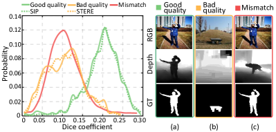
Figure 1. Average probability distributions (solid curves) of edge Dice coefficients computed from “Good quality”, “Bad quality”, and “Mismatch” subsets (10 times random sampling), as well as the probability distributions (dash curves) of the whole STERE and SIP datasets. The right images show three examples from the three subsets, respectively.

An efficiency-oriented model should aim to significantly decrease the number of operations and memory needed while retaining decent accuracy (Sandler et al., 2018). In light of this, several efficiency-oriented RGB-D SOD models have emerged with specific considerations. For example, (Piao et al., 2020; Ji et al., 2020) adopt a depth-free inference strategy for fast speed, while depth cues are only utilized in the training phase. (Zhao et al., 2020; et al., 2020b; Zhang et al., 2020b) choose to design efficient cross-modal fusion modules (Zhao et al., 2020) or light depth backbones (et al., 2020b; Zhang et al., 2020b). However, these methods achieve high efficiency at the sacrifice of state-of-the-art accuracy. One underlying challenge is that their accuracy is likely to degrade when the corresponding models are simplified or reduced.

Motivation. We notice that unstable quality of depth is one key factor which largely influences the accuracy, as mentioned in (Chen et al., 2020; Fan et al., 2020b; Cong et al., 2016). However, very few existing models explicitly take this issue into consideration. We also argue that depth quality is difficult to determine solely according to a depth map (Cong et al., 2016; Chen et al., 2020), because it is tough to judge whether a salient region in the depth map belongs to noise or a target object, as exemplified in Fig. 1 (b). Since RGB-D SOD concerns two paired images as input, i.e., an RGB image and a depth map, our observation is that a high-quality depth map usually has some boundaries well-aligned to the corresponding RGB image. We call this observation “boundary alignment” (BA). To validate such a BA observation, we randomly choose 50 paired samples (tagged as “Good quality” as shown in Fig. 1) from SIP (Fan et al., 2020b) dataset, and also 50 “Bad quality” samples from STERE (Niu et al., 2012) dataset. Choosing such two datasets is based on the general observations of previous works (Fan et al., 2020b; Fu et al., 2020). Additionally, we construct a new set of samples from the “Good quality” set, tagged as “Mismatch”, by randomly mismatching the RGB and depth images of the “Good quality” set, to see if this behavior can be reflected by BA. Note that this behavior actually causes no changes to individual RGB or depth images, therefore having no impact to a depth quality measurement (e.g., (Cong et al., 2016)) that is dependant only on depth itself (often called no-reference metric (Mittal et al., 2012)). To determine boundary alignment, an off-the-shelf edge detector (He et al., 2019) is used to obtain two edge maps from RGB and depth, respectively. We calculate their Dice coefficients (Milletari et al., 2016) as a measure of BA. The probability distributions (average of 10 times random sampling) of Dice coefficients are shown in Fig. 1, where the three sets of samples correspond to different colors. We can see that BA seems a strong evidence for the depth quality issue, and meanwhile for the “Mismatch” set, its Dice coefficients are generally lower than those of the “Good quality” set.

Inspired by the above fact that the alignment of low-level RGB and depth features can somewhat reflect depth quality, we propose a new depth quality-inspired feature manipulation (DQFM) process. The intuition behind DQFM is to assign lower weights to depth features if the quality of depth is bad, effectively avoiding injecting noisy or misleading depth features to improve detection accuracy for efficient models. We also augment DQFM with depth holistic attention, in order to enhance depth features when the depth quality is judged to be good. With the help of DQFM, we explicitly control and enhance the role of depth features during cross-modal fusion. Further in this paper, we embed DQFM into an encoder-decoder framework to obtain an efficient light-weight model called DFM-Net (Depth Feature Manipulation Network), where a tailored depth backbone and a two-stage decoder are designed for efficiency consideration. The main contributions are summarized as follows:

• We propose an efficient depth quality-inspired feature manipulation (DQFM) process, to explicitly control and enhance depth features during cross-modal fusion. DQFM avoids injecting noisy or misleading depth features, and can effectively improve detection accuracy for efficient models.

• Benefited from DQFM, we propose an efficient light-weight model DFM-Net (Depth Feature Manipulation Network), which has a tailored depth backbone and a two-stage decoder.

• Compared to 15 state-of-the-art (SOTA) models, DFM-Net is able to achieve superior accuracy, meanwhile running at 7 FPS on CPU (2.2$\times$ faster than the prior fastest model) with only $\sim$8.5Mb model size (14.9% of the prior smallest).

2. Related Work

The utilization of RGB-D data for SOD has been extensively explored for years. Based on the goal of this paper, in this section, we review general RGB-D SOD methods, as well as previous works on efficient models and depth quality analyses.

2.1. General RGB-D SOD Methods

Traditional methods mainly rely on hand-crafted features (Cheng et al., 2014; et al., 2013; Goferman et al., 2012; Ren et al., 2015). Lately, deep learning-based methods have made great progress and gradually become a mainstream (et al., 2018; Pang et al., 2020; Zhang et al., 2020a; Piao et al., 2019; Fu et al., 2020; Zhang et al., 2020c; Li et al., 2020a; Zhu et al., 2019; Zhao et al., 2019; Fan et al., 2020c; Chen et al., 2019; Ji et al., 2020; Fan et al., 2020b; Zhao et al., 2020). Qu et al. (Qu et al., 2017) first introduced CNNs to infer object saliency from RGB-D data. Zhu et al. (Zhu et al., 2019) designed a master network to process RGB data, together with a sub-network for depth data, and then incorporated depth features into the master network. Fu  et al. (Fu et al., 2020) utilized a Siamese network for simultaneous RGB and depth feature extraction, which discovers the commonality between these two views from a model-based perspective. Zhang  et al. (Zhang et al., 2020a) proposed a probabilistic network via conditional variational auto-encoders to model human annotation uncertainty. Zhang  et al. (Zhang et al., 2020c) proposed a complementary interaction fusion framework to locate salient objects with fine edge details. Liu  et al. (et al., 2020a) introduced a selective self-mutual attention mechanism that can fuse attention learned from both modalities. Li  et al. (Li et al., 2020b) designed a cross-modal weighting network to encourage cross-modal and cross-scale information fusion from low-, middle- and high-level features. Fan  et al. (Fan et al., 2020c) adopted a bifurcated backbone strategy to split multi-level features into student and teacher ones, in order to suppress distractors within low-level layers. Pang  et al. (Pang et al., 2020) provided a new perspective to utilize depth information, in which the depth and RGB features are combined to generate region-aware dynamic filters to guide the decoding in the RGB stream. Li  et al. (Li et al., 2020a) proposed a cross-modality feature modulation module that enhances feature representations by taking depth features as prior. Luo  et al. (Luo et al., 2020) utilized graph-based techniques to design a network architecture for RGB-D SOD. Ji  et al. (Ji et al., 2020) proposed a novel collaborative learning framework, where multiple supervision signals are employed, yielding a depth-free inference method. Zhao  et al. (Zhao et al., 2020) designed a single stream network to directly take a depth map as the fourth channel of an RGB image, and proposed a depth-enhanced dual attention module. A relatively complete survey on RGB-D SOD can be found in (Zhou et al., 2020).

Despite that encouraging detection accuracy has been obtained by the above RGB-D SOD methods, most of them have heavy models and are computationally expensive.

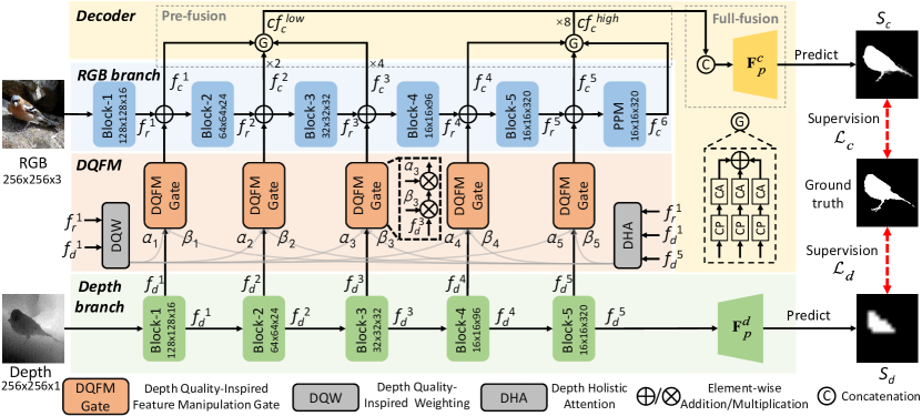
Figure 2. Block diagram of the proposed DFM-Net. Best view in color.

2.2. Efficient RGB-D SOD Methods

Besides the above-mentioned methods, several recent methods attempt to take model efficiency into consideration. Specific techniques are used to reduce high computation brought by multi-modal feature extraction and fusion. Piao  et al. (Piao et al., 2020) employed knowledge distillation for a depth distiller, which aims at transferring depth knowledge obtained from the depth stream to the RGB stream, thus allowing a depth-free inference framework. Chen  et al. (et al., 2020b) constructed a tailored depth backbone to extract complementary features. Such a backbone is much more compact and efficient than classic backbones, e.g., ResNet (He et al., 2016) and VGGNet (Simonyan and Zisserman, 2015). Besides, the method adopts a coarse-to-fine prediction strategy that simplifies the top-down refinement process. The utilized refinement module is in a recurrent manner, further reducing model parameters.

2.3. Depth Quality Analyses in RGB-D SOD

Since the quality of depth often affects model performance, a few researchers have considered the depth quality issue in RGB-D SOD, so as to alleviate the impact of low-quality depth. As early attempts, some works proposed to conduct depth quality assessment from a global perspective and obtained a quality score. Cong et al.  (Cong et al., 2016) first proposed a no-reference depth quality metric (Mittal et al., 2012) to alleviate the contamination of low-quality depth. Later, Fan et al.  (Fan et al., 2020b) used two networks sharing the same structure to process RGB-D input and depth input individually. Depth quality is then evaluated by comparing between the results from the two networks. Cong et al.  (Chen et al., 2020) proposed to predict the depth quality score via a perceptron with high-level RGB and depth features as input. Such a perceptron was trained by scores calculated by comparing thresholded depth maps with ground truth.

Instead of a single quality score, more recently, spatial quality evaluation of depth maps was also considered, in order to find valuable depth region. Wang et al.  (Wang et al., 2020) designed three hand-crafted features to excavate depth following multi-scale methodology. Chen et al.  (Chen et al., 2021) proposed to locate the “Most Valuable Depth Regions” of depth by comparing pseudo GT generated from a sub-network with RGB-D as input, with two saliency maps generated from two sub-networks with RGB/depth as input.

Different from the above existing methods that have high time-space complexity, our depth quality assessment is much more efficient and is more suitable to benefit a light-weight model. Besides, our quality module is end-to-end trainable and is also unsupervised ((Chen et al., 2020, 2021) are supervised for quality estimation).

3. Methodology

3.1. Overview

Fig. 2 shows the block diagram of the proposed DFM-Net, which consists of encoder and decoder parts. For efficiency consideration, our encoder part follows the design in (Fan et al., 2020c), where the RGB branch is simultaneously responsible for RGB feature extraction and cross-modal fusion between RGB and depth features. The decoder part, on the other hand, conducts simple two-stage fusion to generate the final saliency map. More specifically, the encoder consists of an RGB-related branch which is based on MobileNet-v2 (He et al., 2016), a depth-related branch which is a tailored efficient backbone, and also the proposed DQFM. Both branches lead to five feature hierarchies, and the output stride is 2 for each hierarchy except 1 for the last hierarchy. The extracted depth features at a certain hierarchy, after passing through a DQFM gate, are then fused into the RGB branch by simple element-wise addition before being sent to the next hierarchy. Besides, in order to capture multi-scale semantic information, we add a PPM (pyramid pooling module (Zhao et al., 2017)) at the end of the RGB branch. Note that in practice, the DQFM gate contains two successive operations, namely depth quality-inspired weighting (DQW) and depth holistic attention (DHA).

Let the features from the five RGB/depth hierarchies be denoted as $f_{m}^{i}~{}(m\in\{r,d\},i=1,...,5)$, the fused features be denoted as $f_{c}^{i}~{}(i=1,...,5)$, and the features from PPM be denoted as $f_{c}^{6}$. The aforementioned cross-modal feature fusion can be expressed as:

(1) $$f_{c}^{i}=f_{r}^{i}+(\alpha_{i}\otimes\beta_{i}\otimes{f}_{d}^{i}),$$

where $\alpha_{i}$ and $\beta_{i}$ are computed by DQW and DHA to manipulate depth features $f_{d}^{i}$ to be fused, and $\otimes$ denotes element-wise multiplication. After encoding as shown in Fig. 2, $f_{c}^{i}~{}(i=1,...,5)$ and $f_{c}^{6}$ are fed to the subsequent decoder part.

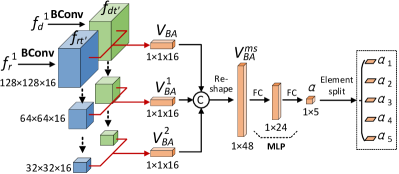
Figure 3. Architecture of DQW (depth quality-inspired weighting). The red line arrows indicate the computation of Eq. 3. The dash line arrows indicate the max pooling with stride 2.

3.2. Depth Quality-Inspired Feature Manipulation (DQFM)

DQFM consists of two key components, namely DQW (depth quality-inspired weighting) and DHA (depth holistic attention), which generate $\alpha_{i}$ and $\beta_{i}$ in Eq. 1, respectively. $\alpha_{i}\in\mathbb{R}^{1}$ is a scalar determining “how much” depth features are involved, while $\beta_{i}\in\mathbb{R}^{k\times k}$ ($k$ is the feature size at hierarchy $i$) is a spatial attention map, deciding “what regions” to focus in the depth features. Below we describe the internal structures of DQW and DHA.

Depth Quality-Inspired Weighting (DQW). Inspired by the aforementioned BA observation in Sec. 1, as shown in Fig. 3, DQW learns the weighting term $\alpha_{i}$ adaptively from low-level features $f_{r}^{1}$ and $f_{d}^{1}$, because such low-level features characterize image edges/boundaries (Zhang et al., 2017). To this end, we first apply convolutions to $f_{r}^{1}$/$f_{d}^{1}$ to obtain transferred features $f_{rt^{\prime}}$/$f_{dt^{\prime}}$, which are expected to capture more edge-related activation:

(2) $$f_{rt^{\prime}}=\textbf{BConv}_{1\times 1}(f_{r}^{1}),~{}f_{dt^{\prime}}=\textbf{BConv}_{1\times 1}(f_{d}^{1}),$$

where $\textbf{BConv}_{1\times 1}(\cdot{})$ denotes a $1\times 1$ convolution with BatchNorm and ReLU activation. To evaluate low-level feature alignment and inspired by Dice coefficient (Milletari et al., 2016), given edge activation $f_{rt^{\prime}}$ and $f_{dt^{\prime}}$, the alignment feature vector $V_{BA}$ that encodes the alignment between $f_{rt^{\prime}}$ and $f_{dt^{\prime}}$ is computed as:

(3) $$V_{BA}=\frac{\textbf{GAP}(f_{rt^{\prime}}\otimes f_{dt^{\prime}})}{\textbf{GAP}(f_{rt^{\prime}}+f_{dt^{\prime}})},$$

where $\textbf{GAP}(\cdot{})$ denotes the global average pooling operation, and $\otimes$ means element-wise multiplication. To make $V_{BA}$ robust against slight edge shifting, we propose to compute $V_{BA}$ at multi-scale and concatenate the results to generate an enhanced vector. As shown in Fig. 3, such multi-scale calculation is conducted by subsequently down-sampling the initial features $f_{rt^{\prime}}$/$f_{dt^{\prime}}$ by max pooling with stride 2, and then computing $V_{BA}^{1},V_{BA}^{2}$ the same as Eq. 3. Suppose $V_{BA}$, $V_{BA}^{1}$, and $V_{BA}^{2}$ are the alignment feature vectors computed from three scales as shown in Fig. 3, the enhanced vector $V_{BA}^{ms}$ is computed as:

(4) $$V_{BA}^{ms}=[V_{BA},V_{BA}^{1},V_{BA}^{2}],$$

where $[\cdot]$ denotes channel concatenation. Next, two fully connected layers are applied to derive $\alpha\in\mathbb{R}^{5}$ from $V_{BA}^{ms}$:

(5) $$\alpha=\textbf{MLP}({V_{BA}^{ms}}),$$

where $\textbf{MLP}(\cdot{})$ denotes a two-layer perceptron with the Sigmoid function at the end. Thus the vector $\alpha$ obtained contains $\alpha_{i}\in(0,1)~{}(i={1,2...,5})$ as its elements. Notably, here we adopt different weighting terms for different hierarchies rather than an identical one. The effectiveness of this strategy is validated in Sec. 4.4.

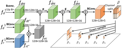
Figure 4. Architecture of DHA (depth holistic attention).

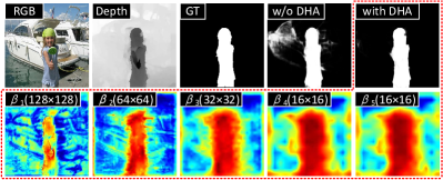
Figure 5. Visualization of holistic attention maps $\beta_{1}\sim\beta_{5}$, as well as the resulting saliency maps with and without DHA.

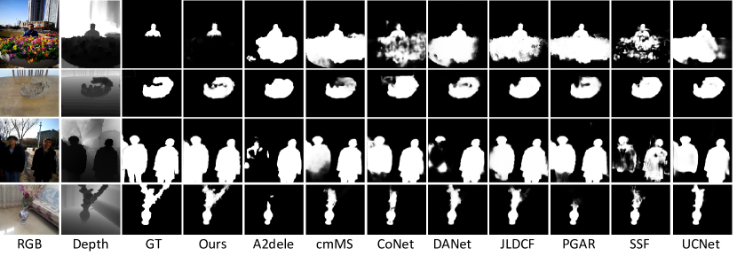
Figure 6. Qualitative comparisons of our method (DFM-Net) with SOTA RGB-D SOD models.

Depth Holistic Attention (DHA). Depth holistic attention (DHA) enhances depth features spatially, by deriving holistic attention map $\beta_{i}$ from the depth stream. Technically as in Fig. 4, we first utilize the highest-level features $f_{d}^{5}$ from the depth stream to locate coarse salient regions (with supervision signals imposed as shown in Fig.  2). To facilitate subsequent pixel-wise operations, we compress and then up-sample $f_{d}^{5}$ into $f_{dht}$, which has the same dimension as $f_{r}^{1}$/$f_{d}^{1}$, formulated as:

(6) $$f_{dht}=\textbf{F}_{UP}^{8}(\textbf{BConv}_{1\times 1}(f_{d}^{5})),$$

where $\textbf{F}_{UP}^{8}$ means 8$\times$ bilinear up-sampling. Then we combine low-level RGB and depth features to recalibrate $f_{dht}$. Similar to the computation of $V_{BA}$, we first transfer $f_{r}^{1}$/$f_{d}^{1}$ to $f_{rt^{\prime\prime}}$/$f_{dt^{\prime\prime}}$ as in DQW. The resulting features are element-wisely multiplied to generate features $f_{ec}$, which emphasizes common edge-related activation. To better model long-range dependencies across low-level and high-level features while maintaining efficiency for DHA, we employ the max pooling operation and dilated convolution to rapidly increase receptive fields. The recalibration process is defined as:

(7) $$\textbf{F}_{rec}(f_{dht})=\textbf{F}_{UP}^{2}\Big{(}\textbf{DConv}_{3\times 3}\big{(}\textbf{F}_{DN}^{2}(f_{dht}+f_{ec})\big{)}\Big{)},$$

where $\textbf{F}_{rec}(\cdot)$ denotes once recalibration process. $\textbf{DConv}_{3\times 3}(\cdot{})$ denotes the $3\times 3$ dilated convolution with stride 1 and dilation rate 2, followed by BatchNorm and ReLU activation. $\textbf{F}_{UP}^{2}(\cdot)/\textbf{F}_{DN}^{2}(\cdot)$ denotes bilinear up-sampling/down-sampling operation to $2/(\frac{1}{2})$ times the original size. As a trade-off between performance and efficiency, we conduct recalibration twice as below:

(8) $$f^{\prime}_{dht}=\textbf{F}_{rec}(f_{dht}),~{}f^{\prime\prime}_{dht}=\textbf{F}_{rec}(f^{\prime}_{dht}),$$

where $f^{\prime}_{dht}$ and $f^{\prime\prime}_{dht}$ represent the features recalibrated once and twice, respectively. Finally, we combine $f^{\prime\prime}_{dht}$ and the previous $f_{ec}$ to achieve holistic attention maps:

(9) $$\beta=\textbf{BConv}_{3\times 3}(f_{ec}+f^{\prime\prime}_{dht}).$$

Note that here the ReLU activation in $\textbf{BConv}_{3\times 3}$ is replaced by the Sigmoid one. Finally we have obtained 5 depth holistic attention maps $\{\beta_{1},\beta_{2},...,\beta_{5}\}$ by down-sampling from $\beta$, severing as spatial enhancement terms for the depth hierarchies. A visual case of DHA is shown in Fig. 5. One can see that $\beta_{1}$ is likely to highlight regions around edges, while $\beta_{5}$ focuses more on the dilated entire object. Generally, irrelevant background clutters in depth features can be somewhat suppressed by multiplying attention maps $\beta_{1}\sim\beta_{5}$.

Table 1. Detailed structure of the proposed tailored depth backbone (TDB), which is based on inverted residual bottleneck blocks (IRB) of MobileNet-V2 (Sandler et al., 2018). About notations, $t$: expansion factor of IRB, $c$: output channels, $n$: times the block is repeated, and $s$: stride of hierarchy, which is applied to the first block of the repeating blocks.

Input	Output	Block	$t$	$c$	$n$	$s$
$256\times 256\times 1$	$128\times 128\times 16$	IRB	3	16	1	2
$128\times 128\times 16$	$64\times 64\times 24$	IRB	3	24	3	2
$64\times 64\times 24$	$32\times 32\times 32$	IRB	3	32	7	2
$32\times 32\times 32$	$16\times 16\times 96$	IRB	2	96	3	2
$16\times 16\times 96$	$16\times 16\times 320$	IRB	2	320	1	1

3.3. Tailored Depth Backbone (TDB)

Usually, depth is less informative than RGB. Hence we consider using a tailored depth backbone (TDB), which is lighter, as a trade-off between efficiency and accuracy. Specifically, we base our TDB on the inverted residual bottleneck blocks (IRB) from MobileNet-V2 (Sandler et al., 2018), and construct a new smaller backbone with reduced channel numbers and stacked blocks, whose structure is detailed in Tab. 1. As a result, our TDB is much lighter than previous light-weight backbones, e.g.,  (Ours: only 0.9Mb, ATSA’s (Zhang et al., 2020b): 6.7Mb, PGAR’s (et al., 2020b): 6.2Mb, MobileNet-V2: 6.9Mb), and meanwhile, its performance is slightly better than MobileNet-V2 (see Sec. 4.4). During training, we embed TDB into DFM-Net without pre-training, and supervision signals are imposed at the end of the backbone to enforce saliency feature learning from depth, as shown in Fig. 2. The coarse prediction result obtained from TDB is formulated as:

(10) $$S_{d}=\textbf{F}_{p}^{d}(f_{d}^{5}),$$

where $S_{d}$ means the coarse prediction from TDB, which is supervised by ground truth (GT). $\textbf{F}_{p}^{d}(\cdot)$ denotes a prediction head consisting of a $1\times 1$ convolution followed by a BatchNorm layer and Sigmoid activation, and also $16\times$ bilinear up-sampling to recover the original input size. The effectiveness of the proposed TDB will be validated in Sec. 4.4 .

Table 2. Quantitative benchmark results. $\uparrow$/$\downarrow$ for a metric denotes that a larger/smaller value is better. Our results are highlighted in bold. The scores/numbers better than ours are underlined (efficient and non-efficient models are labeled separately).

	Metric	PCF	MMCI	CPFP	DMRA	D3Net	JL-DCF	UCNet	SSF	S2MA	CoNet	cmMS	DANet	ATSA	DFM-Net∗	A2dele	PGAR	DFM-Net
		CVPR18	PR19	CVPR19	ICCV19	TNNLS20	CVPR20	CVPR20	CVPR20	CVPR20	ECCV20	ECCV20	ECCV20	ECCV20	Ours	CVPR20	ECCV20	Ours
		(et al., 2018)	(Chen et al., 2019)	(Zhao et al., 2019)	(Piao et al., 2019)	(Fan et al., 2020b)	(Fu et al., 2020)	(Zhang et al., 2020a)	(Zhang et al., 2020c)	(et al., 2020a)	(Ji et al., 2020)	(Li et al., 2020a)	(Zhao et al., 2020)	(Zhang et al., 2020b)	-	(Piao et al., 2020)	(et al., 2020b)	-
	Size (Mb)$\downarrow$	534	930	278	228	530	520	119	125	330	167	430	102	123	93	57	62	8.5
	CPU (ms)$\downarrow$	35762	46886	16946	1521	851	7588	1011	650	1900	667	946	1147	1344	357	313	755	140
	GPU (FPS)$\uparrow$	5	8	6	13	32	9	42	21	25	36	15	32	29	70	120	61	64
SIP	$S_{\alpha}\uparrow$	0.842	0.833	0.850	0.806	0.860	0.879	0.875	0.874	0.878	0.858	0.867	0.878	0.864	0.885	0.829	0.875	0.883
	$F_{\beta}^{\rm max}\uparrow$	0.838	0.818	0.851	0.821	0.861	0.885	0.879	0.880	0.884	0.867	0.871	0.884	0.873	0.890	0.834	0.877	0.887
	$E_{\xi}^{\rm max}\uparrow$	0.901	0.897	0.903	0.875	0.909	0.923	0.919	0.921	0.920	0.913	0.091	0.920	0.911	0.926	0.889	0.914	0.926
	$\mathcal{M}\downarrow$	0.071	0.086	0.064	0.085	0.063	0.051	0.051	0.053	0.054	0.063	0.061	0.054	0.058	0.049	0.070	0.059	0.051
NLPR	$S_{\alpha}\uparrow$	0.874	0.856	0.888	0.899	0.912	0.925	0.920	0.914	0.915	0.908	0.915	0.915	0.907	0.926	0.890	0.918	0.923
	$F_{\beta}^{\rm max}\uparrow$	0.841	0.815	0.867	0.879	0.897	0.916	0.903	0.896	0.902	0.887	0.896	0.903	0.876	0.912	0.875	0.898	0.908
	$E_{\xi}^{\rm max}\uparrow$	0.925	0.913	0.932	0.947	0.953	0.962	0.956	0.953	0.950	0.945	0.949	0.953	0.945	0.961	0.937	0.948	0.957
	$\mathcal{M}\downarrow$	0.044	0.059	0.036	0.031	0.025	0.022	0.025	0.026	0.030	0.031	0.027	0.029	0.028	0.024	0.031	0.028	0.026
NJU2K	$S_{\alpha}\uparrow$	0.877	0.858	0.879	0.886	0.900	0.903	0.897	0.899	0.894	0.895	0.900	0.891	0.901	0.912	0.868	0.906	0.906
	$F_{\beta}^{\rm max}\uparrow$	0.872	0.852	0.877	0.886	0.900	0.903	0.895	0.896	0.889	0.892	0.897	0.880	0.893	0.913	0.872	0.905	0.910
	$E_{\xi}^{\rm max}\uparrow$	0.924	0.915	0.926	0.927	0.950	0.944	0.936	0.935	0.930	0.937	0.936	0.932	0.921	0.950	0.914	0.940	0.947
	$\mathcal{M}\downarrow$	0.059	0.079	0.053	0.051	0.041	0.043	0.043	0.043	0.053	0.047	0.044	0.048	0.040	0.039	0.052	0.045	0.042
RGBD135	$S_{\alpha}\uparrow$	0.842	0.848	0.872	0.900	0.898	0.929	0.934	0.905	0.941	0.910	0.932	0.904	0.907	0.938	0.884	0.894	0.931
	$F_{\beta}^{\rm max}\uparrow$	0.804	0.822	0.846	0.888	0.885	0.919	0.930	0.883	0.935	0.896	0.922	0.894	0.885	0.932	0.873	0.879	0.922
	$E_{\xi}^{\rm max}\uparrow$	0.893	0.928	0.923	0.943	0.946	0.968	0.976	0.941	0.973	0.945	0.970	0.957	0.952	0.973	0.920	0.929	0.972
	$\mathcal{M}\downarrow$	0.049	0.065	0.038	0.030	0.031	0.022	0.019	0.025	0.021	0.029	0.020	0.029	0.024	0.019	0.030	0.032	0.021
LFSD	$S_{\alpha}\uparrow$	0.786	0.787	0.828	0.839	0.825	0.862	0.864	0.859	0.837	0.862	0.849	0.845	0.865	0.870	0.834	0.833	0.865
	$F_{\beta}^{\rm max}\uparrow$	0.775	0.771	0.826	0.852	0.810	0.866	0.864	0.867	0.835	0.859	0.869	0.846	0.862	0.866	0.832	0.831	0.864
	$E_{\xi}^{\rm max}\uparrow$	0.827	0.839	0.863	0.893	0.862	0.901	0.905	0.900	0.873	0.907	0.896	0.886	0.905	0.903	0.874	0.893	0.903
	$\mathcal{M}\downarrow$	0.119	0.132	0.088	0.083	0.095	0.071	0.066	0.066	0.094	0.071	0.074	0.083	0.064	0.068	0.077	0.093	0.072
STERE	$S_{\alpha}\uparrow$	0.875	0.873	0.879	0.835	0.899	0.905	0.903	0.893	0.890	0.908	0.895	0.892	0.897	0.908	0.885	0.903	0.898
	$F_{\beta}^{\rm max}\uparrow$	0.860	0.863	0.874	0.847	0.891	0.901	0.899	0.890	0.882	0.904	0.891	0.881	0.884	0.904	0.885	0.893	0.893
	$E_{\xi}^{\rm max}\uparrow$	0.925	0.927	0.925	0.911	0.938	0.946	0.944	0.936	0.932	0.948	0.937	0.930	0.921	0.948	0.935	0.936	0.941
	$\mathcal{M}\downarrow$	0.064	0.068	0.051	0.066	0.046	0.042	0.039	0.044	0.051	0.040	0.042	0.048	0.039	0.040	0.043	0.044	0.045

3.4. Two-Stage Decoder

Unlike the popular U-Net (Ronneberger et al., 2015) which adopts the hierarchy-by-hierarchy top-down decoding strategy, we propose a simplified two-stage decoder, including pre-fusion and full-fusion, to further improve efficiency. The pre-fusion aims to reduce feature channels and hierarchies, by channel compression and hierarchy grouping, denoted as “CP” and “G” in Fig. 2. Based on the outputs of pre-fusion, the full-fusion further aggregates low-level and high-level hierarchies to generate the final saliency map.

Pre-fusion Stage. We first use $3\times 3$ depth-wise separable convolution (Howard et al., 2017) with BatchNorm and ReLU activation, denoted as $\textbf{DSConv}_{3\times 3}$, to compress the encoder features ($f_{c}^{i},i=1,2...6$) to a unified channel 16, denoted as “CP” in Fig. 2. Then we use the well-known channel attention operator (Hu et al., 2020) $\textbf{F}_{CA}$ to enhance features by weighting different channels, denoted as “CA” in Fig. 2. The above process can be described as:

(11) $$cf_{c}^{i}=\textbf{F}_{CA}(\textbf{DSConv}_{3\times 3}(f_{c}^{i})),$$

where $cf_{c}^{i}$ denotes the compressed and enhanced features. To reduce feature hierarchies, inspired by (Fan et al., 2020c), we group 6 hierarchies into two (i.e., low-level hierarchy and high-level hierarchy) as below:

(12) $$cf_{c}^{low}=\sum_{i=1}^{3}\textbf{F}_{UP}^{2^{i-1}}(cf_{c}^{i}),~{}cf_{c}^{high}=\sum_{i=4}^{6}cf_{c}^{i},$$

where $\textbf{F}_{UP}^{i}$ is bilinear up-sampling to $i$ times the original size.

Full-fusion Stage. Since in the pre-fusion stage, the channel numbers and hierarchies are already reduced, in the full-fusion stage, we directly concatenate high-level and low-level hierarchies, and then feed the concatenation to a prediction head to achieve the final full-resolution prediction map, denoted as:

(13) $$S_{c}=\textbf{F}_{p}^{c}\bigg{(}\big{[}cf_{c}^{low},\textbf{F}_{UP}^{8}(cf_{c}^{high})\big{]}\bigg{)},$$

where $S_{c}$ is the final saliency map, and $\textbf{F}_{p}^{c}(\cdot)$ indicates a prediction head consisting of two $3\times 3$ depth-wise separable convolutions (followed by BatchNorm layers and ReLU activation), a $3\times 3$ convolution with Sigmoid activation, as well as a $2\times$ bilinear up-sampling to recover the original input size.

3.5. Loss Function

The overall loss $\mathcal{L}$ is composed of the final loss $\mathcal{L}_{c}$ and deep supervision for the depth branch loss $\mathcal{L}_{d}$, formulated as:

(14) $$\mathcal{L}=\mathcal{L}_{c}(S_{c},G)+\mathcal{L}_{d}(S_{d},G),$$

where $G$ denotes the ground truth (GT). Similar to previous works (Fu et al., 2020; Fan et al., 2020c; Pang et al., 2020; Fan et al., 2020b), we use the standard cross-entropy loss for $\mathcal{L}_{c}$ and $\mathcal{L}_{d}$.

4. Experiments and Results

4.1. Datasets and Metrics

We conduct experiments on six widely used datasets, including NJU2K (Ju et al., 2014) (1,985 samples), NLPR (Peng et al., 2014) (1,000 samples), STERE (Niu et al., 2012) (1000 samples), RGBD135 (Cheng et al., 2014) (135 samples), LFSD (Li et al., 2014) (100 samples), and SIP (Fan et al., 2020b) (929 samples). Following previous works (Fu et al., 2020; Zhang et al., 2020a; Zhao et al., 2019), we use the same 1,500 samples from NJU2K and 700 samples from NLPR for training, and test on the remaining samples. Four commonly used metrics are used for evaluation, including S-measure ($S_{\alpha}$) (Chen and Fan, 2021), maximum F-measure ($F_{\beta}^{\rm max}$) (Achanta et al., 2009), maximum E-measure ($E_{\xi}^{\rm max}$) (Fan et al., 2018, 2021a), and mean absolute error (MAE, $\mathcal{M}$) (Borji et al., 2015). For efficiency analysis, we report model size (Mb, Mega-bytes), inference time (ms, millisecond) on CPU, and FPS (frame-per-second) on GPU.

Table 3. Ablation analyses for DQFM, where the effectiveness of DQW and DHA is validated. Details are in Sec. 4.4.

#	DQW	DHA	Size	SIP (Fan et al., 2020b)				NLPR (Peng et al., 2014)				NJU2K (Ju et al., 2014)				RGBD135 (Cheng et al., 2014)				LFSD (Li et al., 2014)				STERE (Niu et al., 2012)
			(Mb)	$S_{\alpha}$	$F_{\beta}^{\rm max}$	$E_{\xi}^{\rm max}$	$\mathcal{M}$	$S_{\alpha}$	$F_{\beta}^{\rm max}$	$E_{\xi}^{\rm max}$	$\mathcal{M}$	$S_{\alpha}$	$F_{\beta}^{\rm max}$	$E_{\xi}^{\rm max}$	$\mathcal{M}$	$S_{\alpha}$	$F_{\beta}^{\rm max}$	$E_{\xi}^{\rm max}$	$\mathcal{M}$	$S_{\alpha}$	$F_{\beta}^{\rm max}$	$E_{\xi}^{\rm max}$	$\mathcal{M}$	$S_{\alpha}$	$F_{\beta}^{\rm max}$	$E_{\xi}^{\rm max}$	$\mathcal{M}$
1			8.409	0.849	0.842	0.897	0.070	0.907	0.884	0.946	0.032	0.890	0.887	0.931	0.052	0.929	0.915	0.968	0.025	0.847	0.841	0.883	0.084	0.880	0.872	0.931	0.054
2	✓		8.416	0.878	0.884	0.922	0.054	0.918	0.902	0.957	0.027	0.898	0.898	0.938	0.047	0.932	0.922	0.971	0.022	0.857	0.856	0.896	0.078	0.894	0.886	0.939	0.047
3		✓	8.451	0.861	0.861	0.908	0.063	0.918	0.901	0.953	0.028	0.899	0.896	0.940	0.046	0.921	0.911	0.966	0.024	0.857	0.855	0.895	0.076	0.897	0.891	0.942	0.045
4	✓	✓	8.459	0.883	0.887	0.926	0.051	0.923	0.908	0.957	0.026	0.906	0.910	0.947	0.042	0.931	0.922	0.972	0.021	0.865	0.864	0.903	0.072	0.898	0.893	0.941	0.045

Table 4. Effectiveness of the recalibration process $\textbf{F}_{rec}$ in DHA. The number below “$\textbf{F}_{rec}$” in the table means the times of recalibration. Specifically, zero means that no recalibration is conducted.

#	$\textbf{F}_{rec}$	SIP (Fan et al., 2020b)				NLPR (Peng et al., 2014)				NJU2K (Ju et al., 2014)				RGBD135 (Cheng et al., 2014)				LFSD (Li et al., 2014)				STERE (Niu et al., 2012)
		$S_{\alpha}$	$F_{\beta}^{\rm max}$	$E_{\xi}^{\rm max}$	$\mathcal{M}$	$S_{\alpha}$	$F_{\beta}^{\rm max}$	$E_{\xi}^{\rm max}$	$\mathcal{M}$	$S_{\alpha}$	$F_{\beta}^{\rm max}$	$E_{\xi}^{\rm max}$	$\mathcal{M}$	$S_{\alpha}$	$F_{\beta}^{\rm max}$	$E_{\xi}^{\rm max}$	$\mathcal{M}$	$S_{\alpha}$	$F_{\beta}^{\rm max}$	$E_{\xi}^{\rm max}$	$\mathcal{M}$	$S_{\alpha}$	$F_{\beta}^{\rm max}$	$E_{\xi}^{\rm max}$	$\mathcal{M}$
5	0	0.877	0.881	0.919	0.054	0.920	0.904	0.953	0.027	0.904	0.904	0.943	0.043	0.934	0.924	0.973	0.021	0.855	0.855	0.894	0.076	0.897	0.890	0.940	0.045
6	1	0.872	0.873	0.918	0.056	0.920	0.904	0.957	0.027	0.903	0.902	0.943	0.043	0.929	0.922	0.973	0.023	0.864	0.865	0.902	0.072	0.900	0.893	0.942	0.044
4	2	0.883	0.887	0.926	0.051	0.923	0.908	0.957	0.026	0.906	0.910	0.947	0.042	0.931	0.922	0.972	0.021	0.865	0.864	0.903	0.072	0.898	0.893	0.941	0.045
7	3	0.864	0.868	0.916	0.059	0.921	0.9068	0.957	0.026	0.898	0.897	0.941	0.042	0.917	0.905	0.963	0.025	0.858	0.858	0.896	0.077	0.905	0.897	0.946	0.042

\begin{overpic}[abs,scale={0.55},unit=1mm]{fig/speed} \par\put(53.0,32.0){ \footnotesize \begin{tabular}[]{l|c}\hline\cr\hline\cr\hline\cr Methods&Model size\\ \hline\cr MMCI~{}\cite[citep]{(\@@bibref{AuthorsPhrase1Year}{MMCI}{\@@citephrase{, }}{})}&930\\ PCA~{}\cite[citep]{(\@@bibref{AuthorsPhrase1Year}{PCF}{\@@citephrase{, }}{})}&534\\ D3Net~{}\cite[citep]{(\@@bibref{AuthorsPhrase1Year}{D3Net}{\@@citephrase{, }}{})}&530\\ JL-DCF~{}\cite[citep]{(\@@bibref{AuthorsPhrase1Year}{JLDCF}{\@@citephrase{, }}{})}&520\\ cmMS~{}\cite[citep]{(\@@bibref{AuthorsPhrase1Year}{cmMS}{\@@citephrase{, }}{})}&430\\ S2MA~{}\cite[citep]{(\@@bibref{AuthorsPhrase1Year}{S2MA}{\@@citephrase{, }}{})}&330\\ CPFP~{}\cite[citep]{(\@@bibref{AuthorsPhrase1Year}{CPFP}{\@@citephrase{, }}{})}&278\\ DMRA~{}\cite[citep]{(\@@bibref{AuthorsPhrase1Year}{DRMA}{\@@citephrase{, }}{})}&228\\ CoNet~{}\cite[citep]{(\@@bibref{AuthorsPhrase1Year}{CoNet}{\@@citephrase{, }}{})}&167\\ SSF~{}\cite[citep]{(\@@bibref{AuthorsPhrase1Year}{SSF}{\@@citephrase{, }}{})}&125\\ ASTA~{}\cite[citep]{(\@@bibref{AuthorsPhrase1Year}{ATSA}{\@@citephrase{, }}{})}&123\\ UCNet~{}\cite[citep]{(\@@bibref{AuthorsPhrase1Year}{UCNet}{\@@citephrase{, }}{})}&119\\ DANet~{}\cite[citep]{(\@@bibref{AuthorsPhrase1Year}{DANet}{\@@citephrase{, }}{})}&102\\ {{DFM-Net*}}&{93}\\ \hline\cr PGAR~{}\cite[citep]{(\@@bibref{AuthorsPhrase1Year}{PGAR}{\@@citephrase{, }}{})}&62\\ A2dele~{}\cite[citep]{(\@@bibref{AuthorsPhrase1Year}{A2dele}{\@@citephrase{, }}{})}&57\\ {{DFM-Net}}&{8.5}\\ \hline\cr\hline\cr\hline\cr\end{tabular}} \end{overpic}

Figure 7. Performance visualization. The vertical axis indicates the accuracy ($F_{\beta}^{\rm max}$) on SIP (Fan et al., 2020b). The horizontal axis indicates the CPU speed (FPS). The circle area is proportional to the model size. More details refer to Tab. 2.

4.2. Implementation Details

Experiments are conducted on a workstation with Intel Core i7-8700 CPU, Nvidia GTX 1080Ti GPU with CUDA 10.1. We implement DFM-Net by PyTorch (Paszke et al., 2019), and RGB and depth images are both resized to $256\times 256$ for input. For testing, the inference time on CPU and FPS on GPU is obtained by averaging 100 times inference with batch size 1, and no any data augmentation or post processing is used. For training, in order generalize the network on limited training samples, following  (Fan et al., 2020c), we apply various data augmentation techniques  i.e., random translation/cropping, horizontal flipping, color enhancement and so on. We train DFM-Net for 300 epochs on a single 1080Ti GPU, taking about 4 hours. The initial learning rate is set as 1e-4 for Adam optimizer, and the batch size is 10. The poly learning rate policy is used, where the power is set to 0.9.

4.3. Quantitative and Qualitative Comparisons

Since we cannot expect that an extremely light-weight model can always outperform existing non-efficient models (which are much larger), we have also extended DFM-Net to obtain a larger but more powerful model called DFM-Net*, by replacing MobileNet-v2 used in the RGB branch with ResNet-34 (He et al., 2016). Then to align the features from the RGB branch to those from TDB, slight modifications are made. Results of DFM-Net and DFM-Net*, compared to 15 state-of-the-art (SOTA) models including PCF (et al., 2018), MMCI (Chen et al., 2019), CPFP (Zhao et al., 2019), DRMA (Piao et al., 2019), D3Net (Fan et al., 2020b), JL-DCF (Fu et al., 2020), UCNet (Zhang et al., 2020a), SSF (Zhang et al., 2020c), S2MA (et al., 2020a), CoNet (Ji et al., 2020), cmMS (Li et al., 2020a), DANet (Zhao et al., 2020), ATSA (Zhang et al., 2020b), A2dele (Piao et al., 2020) and PGAR (et al., 2020b), can be found in Tab. 2.

As shown in Tab. 2, DFM-Net surpasses existing efficient models A2dele (Piao et al., 2020) and PGAR (et al., 2020b) significantly on detection accuracy and model size, as well as CPU speed. It runs at 140ms on CPU, which is the fastest among all the contenders, with only $\sim$8.5Mb model size (14.9% of that of A2dele). About GPU speed, DFM-Net ranks the second after A2dele (Piao et al., 2020). This is because the depth-wise separable convolution layers, which have been extensively used in MobileNet-v2 and TDB, cannot be fully accelerated on GPU in the current implementation (Williams et al., 2009; Hong et al., 2021). On the other hand, one can see that DFM-Net* achieves SOTA performance when compared to existing non-efficient models, with absolutely the fastest CPU/GPU speed and the smallest model size. Visual comparisons with representative methods are shown in Fig. 6, where our results are closer to the ground truth (GT).

To better reflect the advantages of the proposed method, as shown in Fig. 7, we visualize all models by plotting their accuracy ($F_{\beta}^{\rm max}$ on SIP dataset, the vertical axis), w.r.t. their CPU speed (FPS is used here for better visualization, the horizontal axis) and model size (proportional to the circle diameter). It is clearly seen that DFM-Net and DFM-Net* can rank the most upper right with very small circles, indicating that our method can perform well in terms of both efficiency and accuracy when compared to existing techniques.

Table 5. DQFM gating strategy: using identical (only one) $\alpha_{i}$ and $\beta_{i}$ vs. using multiple (five different) $\alpha_{i}$ and $\beta_{i}$.

#	Strategy	SIP (Fan et al., 2020b)				NLPR (Peng et al., 2014)				NJU2K (Ju et al., 2014)				RGBD135 (Cheng et al., 2014)				LFSD (Li et al., 2014)				STERE (Niu et al., 2012)
		$S_{\alpha}$	$F_{\beta}^{\rm max}$	$E_{\xi}^{\rm max}$	$\mathcal{M}$	$S_{\alpha}$	$F_{\beta}^{\rm max}$	$E_{\xi}^{\rm max}$	$\mathcal{M}$	$S_{\alpha}$	$F_{\beta}^{\rm max}$	$E_{\xi}^{\rm max}$	$\mathcal{M}$	$S_{\alpha}$	$F_{\beta}^{\rm max}$	$E_{\xi}^{\rm max}$	$\mathcal{M}$	$S_{\alpha}$	$F_{\beta}^{\rm max}$	$E_{\xi}^{\rm max}$	$\mathcal{M}$	$S_{\alpha}$	$F_{\beta}^{\rm max}$	$E_{\xi}^{\rm max}$	$\mathcal{M}$
8	Identical	0.880	0.884	0.924	0.053	0.922	0.907	0.958	0.026	0.901	0.901	0.944	0.044	0.924	0.911	0.961	0.024	0.859	0.857	0.899	0.073	0.898	0.892	0.942	0.045
4	Multiple	0.883	0.887	0.926	0.051	0.923	0.908	0.957	0.026	0.906	0.910	0.947	0.042	0.931	0.922	0.972	0.021	0.865	0.864	0.903	0.072	0.898	0.893	0.941	0.045

Table 6. Performance of the proposed TDB (tailored depth backbone) against MobileNet-V2. Details are in Sec. 4.4.

#	Depth	Size	SIP (Fan et al., 2020b)				NLPR (Peng et al., 2014)				NJU2K (Ju et al., 2014)				RGBD135 (Cheng et al., 2014)				LFSD (Li et al., 2014)				STERE (Niu et al., 2012)
	backbone	(Mb)	$S_{\alpha}$	$F_{\beta}^{\rm max}$	$E_{\xi}^{\rm max}$	$\mathcal{M}$	$S_{\alpha}$	$F_{\beta}^{\rm max}$	$E_{\xi}^{\rm max}$	$\mathcal{M}$	$S_{\alpha}$	$F_{\beta}^{\rm max}$	$E_{\xi}^{\rm max}$	$\mathcal{M}$	$S_{\alpha}$	$F_{\beta}^{\rm max}$	$E_{\xi}^{\rm max}$	$\mathcal{M}$	$S_{\alpha}$	$F_{\beta}^{\rm max}$	$E_{\xi}^{\rm max}$	$\mathcal{M}$	$S_{\alpha}$	$F_{\beta}^{\rm max}$	$E_{\xi}^{\rm max}$	$\mathcal{M}$
9	MoblieNet-V2	6.9	0.879	0.886	0.923	0.054	0.919	0.904	0.954	0.027	0.906	0.908	0.948	0.042	0.930	0.922	0.969	0.022	0.864	0.864	0.902	0.070	0.893	0.889	0.942	0.046
4	Tailored	0.9	0.883	0.887	0.926	0.051	0.923	0.908	0.957	0.026	0.906	0.910	0.947	0.042	0.931	0.922	0.972	0.021	0.865	0.864	0.903	0.072	0.898	0.893	0.941	0.045

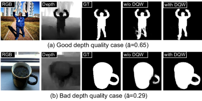
Figure 8. Visualized examples of setting #3 (w/o DQW) and #4 (with DQW) for good (a) and bad (b) depth quality cases. $\overline{\alpha}$ denotes the average of $\alpha_{1}\sim\alpha_{5}$, which can be deemed as an indicator for depth quality.

4.4. Ablation Studies

We conduct thorough ablation studies on six datasets by removing or replacing components from the full implementation of DFM-Net.

Effectiveness of DQFM. DQFM consists of two key components, namely DQW and DHA. Tab. 3 shows different configurations by ablating DQW/DHA. In detail, #1 denotes a baseline model which has removed both DQW and DHA from DFM-Net. Configuration #2 and #3 mean having either one component, while #4 means the full model of DFM-Net. Basically, from Tab. 3 one can see that incorporating either DQW and DHA into the baseline model #1 leads to consistent improvement on almost all datasets. Besides, comparing #2/#3 to #4, we see that employing both DQW and DHA can further enhance the results, demonstrating the complementary effect between DQW and DHA. The underlying reason could be that, although DHA is able to enhance potential target regions in the depth, it is unavoidable to make some mistakes (e.g., highlight wrong regions) especially in low depth quality cases. Luckily, DQW somewhat relieves such a side-effect because in the meantime it assigns low global weights to depth features. In all, these two components can work cooperatively to improve the robustness of the network, as we mentioned in Sec. 3.2. Last but not least, from the model sizes of different configurations shown in Tab. 3 , the extra model parameters for introducing DQW and DHA are quite few. This rightly meets our goal and implies that they could potentially become universal components for light-weight models in the future.

In Fig. 8, we show visual examples of setting #3 (namely without DQW) and #4. We also visualize the magnitudes of $\alpha$, namely the mean value $\overline{\alpha}$ of $\alpha_{1}\sim\alpha_{5}$. From Fig. 8 (a) and (b), we can see that incorporating DQW does help improve detection accuracy, and practically, DQW is able to function as expected, namely rendering the good quality case with higher weights ($\overline{\alpha}=0.65$), and vice versa ($\overline{\alpha}=0.29$). In the good quality case (a), it is difficult to distinguish between the shadow and the man’s legs in the RGB view, but this can be done easily in the depth view. Incorporating DQW to give more emphasis to depth features, therefore, can help better separate the entire human body from the shadow. In the bad quality case (b), although in the depth view the cup handle is much blurry, the impact of misleading depth has been alleviated, and the whole object still can be detected out accurately.

Recalibration in DHA. As described in Sec. 3.2, in DHA, we utilize operation $\textbf{F}_{rec}$ to recalibrate the coarse information from high-level depth features. To validate the necessity of using $\textbf{F}_{rec}$, we experiment with different times (from 0 to 3) of using $\textbf{F}_{rec}$. These variants are denoted as #5, #6, #4, and #7 in Tab. 4. Note that #4 corresponds to the default implementation of DFM-Net. From Tab. 4, we can see that #4 (recalibrate twice) achieves the overall best performance. The underlying reason should be that, appropriate usage of $\textbf{F}_{rec}$ can expand the coverage areas of attention maps to make conservative filtering for object edges as well as some inaccurately located objects, but too large receptive field leads to over-dilated attention regions that are less informative. This is the reason why when the times increase to 3, the performance starts to degenerate on most datasets, except on STERE whose depth quality is generally low, which easily leads to inaccurate attention location.

DQFM Gating Strategy. As we mentioned in Sec. 3.2, we adopt a multi-variable strategy for $\alpha_{i}$ and $\beta_{i}$. To validate this strategy, we compare it to the single-variable strategy, namely using identical (only one) $\alpha_{i}$ and $\beta_{i}$. Tab. 5 shows the results, from which it can be seen that our proposed multi-variable strategy is better, because it somewhat increases the network flexibility by rendering different hierarchies with different quality weights and attention maps.

Tailored Depth Backbone. The effectiveness of TDB is validated by comparing it to MobileNet-V2. We implement a configuration #9 by switching TDB directly to MobileNet-V2, while maintaining all other settings unchanged. Evaluation results are shown in Tab. 6. We can see that our tailored depth backbone is more efficient (0.9Mb vs. MobileNet-V2’s 6.9Mb) and also more accurate (with noticeable gains) than MobileNet-V2 when utilized in DFM-Net. This demonstrates the feasibility of using a lighter backbone to process depth data for efficiency purpose.

5. Conclusion

In this paper, we propose an efficient RGB-D SOD model called DFM-Net, characterized by the the DQFM process to explicitly control and enhance depth features during cross-modal fusion. The two key components in DQFM, namely DQW and DHA, are validated by comprehensive ablation experiments. The experimental results show that DQW and DHA are both essential for obtaining higher detection accuracy with very few model parameters added on. Besides, a tailored depth backbone and a two-stage decoder are elaborately designed to further improve the efficiency of DFM-Net. Our DFM-Net achieves new state-of-the-art records on light-weight model size as well as CPU speed, meanwhile retaining decent accuracy. In the future, it is very attractive to apply DFM-Net on some embedding or mobile systems that process RGB-D data.

References

- (1)
- Achanta et al. (2009) R. Achanta, S. Hemami, F. J. Estrada, and S. Süsstrunk. 2009. Frequency-tuned salient region detection. In CVPR. 1597–1604.
- Borji et al. (2015) A. Borji, M. Cheng, Huaizu Jiang, and J. Li. 2015. Salient Object Detection: A Benchmark. IEEE TIP 24 (2015), 5706–5722.
- Chen et al. (2021) C. Chen, J. Wei, C. Peng, and H. Qin. 2021. Depth-Quality-Aware Salient Object Detection. IEEE Transactions on Image Processing PP, 99 (2021), 1–1.
- Chen et al. (2019) Hao Chen, Youfu Li, and Dan Su. 2019. Multi-modal fusion network with multi-scale multi-path and cross-modal interactions for RGB-D salient object detection. Pattern Recognition 86 (2019), 376–385.
- Chen and Fan (2021) Ming-Ming Chen and Deng-Ping Fan. 2021. Structure-measure: A New Way to Evaluate Foreground Maps. IJCV (2021).
- Chen et al. (2020) Zuyao Chen, Runmin Cong, Q. Xu, and Qingming Huang. 2020. DPANet: Depth Potentiality-Aware Gated Attention Network for RGB-D Salient Object Detection. IEEE TIP (2020).
- Cheng et al. (2014) Yupeng Cheng, Huazhu Fu, Xingxing Wei, Jiangjian Xiao, and Xiaochun Cao. 2014. Depth enhanced saliency detection method. In ICIMCS. 23–27.
- Cong et al. (2016) Runmin Cong, Jianjun Lei, Changqing Zhang, Q. Huang, Xiaochun Cao, and C. Hou. 2016. Saliency Detection for Stereoscopic Images Based on Depth Confidence Analysis and Multiple Cues Fusion. IEEE Signal Processing Letters 23 (2016), 819–823.
- et al. (2013) Ciptadi et al. 2013. An in depth view of saliency. In BMVC. Georgia Institute of Technology, 112.
- et al. (2018) H. Chen et al. 2018. Progressively Complementarity-Aware Fusion Network for RGB-D Salient Object Detection. In CVPR. 3051–3060.
- et al. (2020a) Nian Liu et al. 2020a. Learning Selective Self-Mutual Attention for RGB-D Saliency Detection. In CVPR. 13756–13765.
- et al. (2020b) Shuhan Chen et al. 2020b. Progressively Guided Alternate Refinement Network for RGB-D Salient Object Detection. In ECCV. 520–538.
- Fan et al. (2018) Deng-Ping Fan, Cheng Gong, Yang Cao, Bo Ren, Ming-Ming Cheng, and Ali Borji. 2018. Enhanced-alignment Measure for Binary Foreground Map Evaluation. In IJCAI. 698–704.
- Fan et al. (2021a) Deng-Ping Fan, Ge-Peng Ji, Xuebin Qin, and Ming-Ming Cheng. 2021a. Cognitive Vision Inspired Object Segmentation Metric and Loss Function (in Chinese). SCIENTIA SINICA Informationis (2021). https://doi.org/10.1360/SSI-2020-0370
- Fan et al. (2020a) Deng-Ping Fan, Ge-Peng Ji, Tao Zhou, Geng Chen, Huazhu Fu, Jianbing Shen, and Ling Shao. 2020a. PraNet: Parallel Reverse Attention Network for Polyp Segmentation. MICCAI (2020).
- Fan et al. (2021b) Deng-Ping Fan, Tengpeng Li, Zheng Lin, Ge-Peng Ji, Dingwen Zhang, Ming-Ming Cheng, Huazhu Fu, and Jianbing Shen. 2021b. Re-thinking co-salient object detection. TPAMI (2021).
- Fan et al. (2020b) Deng-Ping Fan, Zheng Lin, Zhao Zhang, Menglong Zhu, and Ming-Ming Cheng. 2020b. Rethinking RGB-D salient object detection: Models, datasets, and large-scale benchmarks. IEEE TNNLS (2020).
- Fan et al. (2020c) Deng-Ping Fan, Yingjie Zhai, Ali Borji, Jufeng Yang, and Ling Shao. 2020c. BBS-Net: RGB-D Salient Object Detection with a Bifurcated Backbone Strategy Network. In ECCV. 275–292.
- Fu et al. (2020) Keren Fu, Deng-Ping Fan, Ge-Peng Ji, and Qijun Zhao. 2020. JL-DCF: Joint Learning and Densely-Cooperative Fusion Framework for RGB-D Salient Object Detection. In CVPR. 3052–3062.
- Fu et al. (2021) Keren Fu, Deng-Ping Fan, Ge-Peng Ji, Qijun Zhao, Jianbing Shen, and Ce Zhu. 2021. Siamese network for rgb-d salient object detection and beyond. IEEE TPAMI (2021). https://doi.org/10.1109/TPAMI.2021.3073689
- Goferman et al. (2012) Stas Goferman, L. Zelnik-Manor, and A. Tal. 2012. Context-Aware Saliency Detection. IEEE TPMAI 34 (2012), 1915–1926.
- Guo and Zhang (2010) Chenlei Guo and Liming Zhang. 2010. A Novel Multiresolution Spatiotemporal Saliency Detection Model and Its Applications in Image and Video Compression. TEEE TIP 19, 1 (2010), 185–198.
- He et al. (2019) Jianzhong He, Shiliang Zhang, Ming Yang, Yanhu Shan, and Tiejun Huang. 2019. Bi-Directional Cascade Network for Perceptual Edge Detection. In CVPR. 3823–3832.
- He et al. (2016) Kaiming He, Xiangyu Zhang, Shaoqing Ren, and Jian Sun. 2016. Deep Residual Learning for Image Recognition. In CVPR. 25–32.
- Hong et al. (2021) Yuanduo Hong, Huihui Pan, Weichao Sun, Senior Member, and Yisong Jia. 2021. Deep Dual-resolution Networks for Real-time and Accurate Semantic Segmentation of Road Scenes. arXiv:2101.06085 [cs.CV]
- Howard et al. (2017) Andrew G. Howard, Menglong Zhu, Bo Chen, Dmitry Kalenichenko, Weijun Wang, Tobias Weyand, Marco Andreetto, and Hartwig Adam. 2017. MobileNets: Efficient Convolutional Neural Networks for Mobile Vision Applications. arXiv:1704.04861 [cs.CV]
- Hu et al. (2020) Jie Hu, L. Shen, Samuel Albanie, G. Sun, and Enhua Wu. 2020. Squeeze-and-Excitation Networks. IEEE TPAMI 42 (2020), 2011–2023.
- Ji et al. (2021) Ge-Peng Ji, Yu-Cheng Chou, Deng-Ping Fan, Geng Chen, Debesh Jha, Huazhu Fu, and Ling Shao. 2021. Progressively Normalized Self-Attention Network for Video Polyp Segmentation. In MICCAI.
- Ji et al. (2020) Wei Ji, Jingjing Li, Miao Zhang, Yongri Piao, and Huchuan Lu. 2020. Accurate RGB-D Salient Object Detection via Collaborative Learning. In ECCV. 52–69.
- Jiang et al. (2020) Yao Jiang, Tao Zhou, Ge-Peng Ji, Keren Fu, Qijun Zhao, and Deng-Ping Fan. 2020. Light Field Salient Object Detection: A Review and Benchmark. arXiv preprint arXiv:2010.04968 (2020).
- Ju et al. (2014) Ran Ju, L. Ge, W. Geng, T. Ren, and Gangshan Wu. 2014. Depth saliency based on anisotropic center-surround difference. In ICIP. 1115–1119.
- Li et al. (2020a) Chongyi Li, Runmin Cong, Piao Yongri, Xu Qianqian, and Chen Change Loy. 2020a. RGB-D salient object detection with cross-modality modulation and selection. In ECCV. 225–241.
- Li et al. (2020b) Gongyang Li, Zhusong Liu, L. Ye, Yang Wang, and H. Ling. 2020b. Cross-Modal Weighting Network for RGB-D Salient Object Detection. In ECCV. 665–681.
- Li et al. (2014) Nianyi Li, J. Ye, Y. Ji, Haibin Ling, and J. Yu. 2014. Saliency Detection on Light Field. IEEE TPAMI 39 (2014), 1605–1616.
- Luo et al. (2020) Ao Luo, Xin Li, Fan Yang, Zhicheng Jiao, Hong Cheng, and Siwei Lyu. 2020. Cascade Graph Neural Networks for RGB-D Salient Object Detection. In ECCV. 346–364.
- Milletari et al. (2016) Fausto Milletari, Nassir Navab, and Seyed-Ahmad Ahmadi. 2016. V-Net: Fully Convolutional Neural Networks for Volumetric Medical Image Segmentation. 3DV (2016), 565–571.
- Mittal et al. (2012) Anish Mittal, Anush K. Moorthy, and A. Bovik. 2012. No-Reference Image Quality Assessment in the Spatial Domain. IEEE TIP 21 (2012), 4695–4708.
- Niu et al. (2012) Y. Niu, Yujie Geng, X. Li, and Feng Liu. 2012. Leveraging stereopsis for saliency analysis. In CVPR. 454–461.
- Pang et al. (2020) Youwei Pang, Lihe Zhang, Xiaoqi Zhao, and Huchuan Lu. 2020. Hierarchical Dynamic Filtering Network for RGB-D Salient Object Detection. In ECCV. 235–252.
- Paszke et al. (2019) Adam Paszke, S. Gross, Francisco Massa, A. Lerer, James Bradbury, Gregory Chanan, Trevor Killeen, Z. Lin, N. Gimelshein, L. Antiga, Alban Desmaison, Andreas Köpf, Edward Yang, Zach DeVito, Martin Raison, Alykhan Tejani, Sasank Chilamkurthy, B. Steiner, Lu Fang, Junjie Bai, and Soumith Chintala. 2019. PyTorch: An Imperative Style, High-Performance Deep Learning Library. In NeurIPS.
- Peng et al. (2014) Houwen Peng, B. Li, Weihua Xiong, W. Hu, and R. Ji. 2014. RGBD Salient Object Detection: A Benchmark and Algorithms. In ECCV. 92–109.
- Piao et al. (2019) Yongri Piao, Wei Ji, Jingjing Li, Miao Zhang, and Huchuan Lu. 2019. Depth-induced multi-scale recurrent attention network for saliency detection. In ICCV. 7254–7263.
- Piao et al. (2020) Yongri Piao, Zhengkun Rong, Miao Zhang, Weisong Ren, and Huchuan Lu. 2020. A2dele: Adaptive and Attentive Depth Distiller for Efficient RGB-D Salient Object Detection. In CVPR. 9060–9069.
- Qu et al. (2017) Liangqiong Qu, Shengfeng He, Jiawei Zhang, Jiandong Tian, Y. Tang, and Q. Yang. 2017. RGBD Salient Object Detection via Deep Fusion. IEEE TIP 26 (2017), 2274–2285.
- Ren et al. (2015) Jianqiang Ren, Xiaojin Gong, Lu Yu, Wenhui Zhou, and Michael Ying Yang. 2015. Exploiting global priors for RGB-D saliency detection. In CVPR. 25–32.
- Ronneberger et al. (2015) O. Ronneberger, P. Fischer, and T. Brox. 2015. U-Net: Convolutional Networks for Biomedical Image Segmentation. In MICCAI. 234–241.
- Sandler et al. (2018) Mark Sandler, A. Howard, Menglong Zhu, A. Zhmoginov, and Liang-Chieh Chen. 2018. MobileNetV2: Inverted Residuals and Linear Bottlenecks. In CVPR. 4510–4520.
- Simonyan and Zisserman (2015) Karen Simonyan and Andrew Zisserman. 2015. Very Deep Convolutional Networks for Large-Scale Image Recognition. ICLR (2015).
- Wang et al. (2021) Wenguan Wang, Qiuxia Lai, Huazhu Fu, J. Shen, and Haibin Ling. 2021. Salient Object Detection in the Deep Learning Era: An In-Depth Survey. IEEE TPAMI (2021).
- Wang et al. (2018) Wenguan Wang, J. Shen, Ruigang Yang, and F. Porikli. 2018. Saliency-Aware Video Object Segmentation. IEEE TPAMI 40 (2018), 20–33.
- Wang et al. (2020) X. Wang, S. Li, C. Chen, A. Hao, and H. Qin. 2020. Depth Quality-aware Selective Saliency Fusion for RGB-D Image Salient Object Detection. Neurocomputing 432 (2020).
- Williams et al. (2009) S. Williams, A. Waterman, and David A. Patterson. 2009. Roofline: an insightful visual performance model for multicore architectures. Commun. ACM 52 (2009), 65–76.
- Zhai et al. (2020) Yingjie Zhai, Deng-Ping Fan, Jufeng Yang, Ali Borji, Ling Shao, Junwei Han, and Liang Wang. 2020. Bifurcated backbone strategy for RGB-D salient object detection. arXiv preprint arXiv:2007.02713 (2020).
- Zhang et al. (2020a) Jing Zhang, Deng-Ping Fan, Yuchao Dai, Saeed Anwar, Fatemeh Sadat Saleh, Tong Zhang, and Nick Barnes. 2020a. UC-Net: Uncertainty Inspired RGB-D Saliency Detection via Conditional Variational Autoencoders. In CVPR. 8582–8519.
- Zhang et al. (2021a) Jing Zhang, Deng-Ping Fan, Yuchao Dai, Saeed Anwar, Fatemeh Saleh, Sadegh Aliakbarian, and Nick Barnes. 2021a. Uncertainty Inspired RGB-D Saliency Detection. IEEE TPAMI (2021). https://doi.org/10.1109/TPAMI.2021.3073564
- Zhang et al. (2020b) Miao Zhang, S. Fei, Jie Liu, Shuang Xu, Yongri Piao, and Huchuan Lu. 2020b. Asymmetric Two-Stream Architecture for Accurate RGB-D Saliency Detection. In ECCV. 374–390.
- Zhang et al. (2020c) Miao Zhang, Weisong Ren, Yongri Piao, Zhengkun Rong, and Huchuan Lu. 2020c. Select, Supplement and Focus for RGB-D Saliency Detection. In CVPR. 3472–3481.
- Zhang et al. (2019) Pingping Zhang, Wei Liu, Dong Wang, Yinjie Lei, and Huchuan Lu. 2019. Non-rigid object tracking via deep multi-scale spatial-temporal discriminative saliency maps. Pattern Recognition 100 (2019), 107130.
- Zhang et al. (2017) Pingping Zhang, D. Wang, H. Lu, Hongyu Wang, and X. Ruan. 2017. Amulet: Aggregating Multi-level Convolutional Features for Salient Object Detection. In ICCV. 202–211.
- Zhang et al. (2021b) Zhao Zhang, Zheng Lin, Jun Xu, Wen-Da Jin, Shao-Ping Lu, and Deng-Ping Fan. 2021b. Bilateral attention network for RGB-D salient object detection. IEEE TIP 30 (2021), 1949–1961.
- Zhao et al. (2017) Hengshuang Zhao, J. Shi, Xiaojuan Qi, Xiaogang Wang, and J. Jia. 2017. Pyramid Scene Parsing Network. In CVPR. 6230–6239.
- Zhao et al. (2019) Jia-Xing Zhao, Yang Cao, Deng-Ping Fan, Ming-Ming Cheng, Xuan-Yi Li, and Le Zhang. 2019. Contrast prior and fluid pyramid integration for RGBD salient object detection. In CVPR. 3927–3936.
- Zhao et al. (2020) Xiaoqi Zhao, Lihe Zhang, Youwei Pang, Huchuan Lu, and Lei Zhang. 2020. A Single Stream Network for Robust and Real-time RGB-D Salient Object Detection. In ECCV. 520–538.
- Zhou et al. (2020) Tao Zhou, Deng-Ping Fan, Ming-Ming Cheng, Jianbing Shen, and Ling Shao. 2020. RGB-D Salient Object Detection: A Survey. Computational Visual Media 7 (2020), 37–69.
- Zhu et al. (2019) Chunbiao Zhu, Xing Cai, Kan Huang, Thomas H Li, and Ge Li. 2019. PDNet: Prior-model guided depth-enhanced network for salient object detection. In ICME. 199–204.