Optimal Binary Classification Beyond Accuracy

Abstract

The vast majority of statistical theory on binary classification characterizes performance in terms of accuracy. However, accuracy is known in many cases to poorly reflect the practical consequences of classification error, most famously in imbalanced binary classification, where data are dominated by samples from one of two classes. The first part of this paper derives a novel generalization of the Bayes-optimal classifier from accuracy to any performance metric computed from the confusion matrix. Specifically, this result (a) demonstrates that stochastic classifiers sometimes outperform the best possible deterministic classifier and (b) removes an empirically unverifiable absolute continuity assumption that is poorly understood but pervades existing results. We then demonstrate how to use this generalized Bayes classifier to obtain regret bounds in terms of the error of estimating regression functions under uniform loss. Finally, we use these results to develop some of the first finite-sample statistical guarantees specific to imbalanced binary classification. Specifically, we demonstrate that optimal classification performance depends on properties of class imbalance, such as a novel notion called Uniform Class Imbalance, that have not previously been formalized. We further illustrate these contributions numerically in the case of $k$-nearest neighbor classification.

1 Introduction

Many binary classification problems exhibit class imbalance, in which one of the two classes vastly outnumbers the other. Classifiers that perform well with balanced classes routinely fail for imbalanced classes, and developing reliable techniques for classification in the presence of severe class imbalance remains a challenging area of research (He and Ma, 2013; Krawczyk, 2016; Fernández et al., 2018). Many practical approaches have been proposed to improve performance under class imbalance, including reweighting plug-in estimates of class probabilities (Lewis, 1995), resampling data to improve class imbalance (Chawla et al., 2002), or reformulating classification algorithms to optimize different performance metrics (Dembczynski et al., 2013; Fathony and Kolter, 2019; Joachims, 2005). Extensive discussion of practical methods for handling class imbalance are surveyed in the books of He and Ma (2013) and Fernández et al. (2018).

Despite the pervasive challenge of class imbalance, our theoretical understanding of class imbalance is limited. The vast majority of theoretical performance guarantees for classification characterize classification accuracy or, equivalently, misclassification risk (Mohri et al., 2018), which is typically an uninformative measure of performance for imbalanced classes. Under measures that are used with imbalanced classes in practice, such as precision, recall, $F_{\beta}$ scores, and class-weighted scores (Van Rijsbergen, 1974, 1979), existing theoretical guarantees are limited to statistical consistency, in that the algorithm under consideration asymptotically optimizes the metric of choice (Koyejo et al., 2014; Menon et al., 2013; Narasimhan et al., 2014); specifically, there is no finite-sample theory that would allow comparison of an algorithm’s performance to that of other algorithms or to theoretically optimal performance levels. Additionally, existing theory for classification does not explicitly model the effects of class imbalance, especially severe imbalance (i.e., as the proportion of samples from the rare class vanishes), and hence sheds little light on how severe imbalance influences optimal classification.

This paper provides two main contributions. First, in Section 4, we provide a novel characterization of classifiers optimizing general performance metrics that are functions of a classifier’s confusion matrix. This characterization generalizes a classical result, that the Bayes classifier optimizes classification accuracy, to a much larger class of performance measures, including those commonly used in imbalanced classification, while relaxing certain empirically unverifiable distributional assumptions that pervade existing such results. Interestingly, we show that, in general, a Bayes classifier always exists if one considers stochastic classifiers, but not if one considers only deterministic classifiers. We then use this result to provide relative performance guarantees under these more general performance measures, in terms of the error of estimating the class probability (regression) function under uniform ($\mathcal{L}_{\infty}$) loss.

This motivates our second main contribution: an analysis of $k$-nearest neighbor ($k$NN) classification under uniform loss. In doing so, we also propose an explicit model of a sub-type of class imbalance, which we call Uniform Class Imbalance, and we show that the $k$NN classifier behaves quite differently under Uniform Class Imbalance than under other sub-types of class imbalance. To the best of our knowledge, such sub-types of class imbalance have not previously been distinguished in either the theoretical or practical literature, and we hope that identifying such relevant features of imbalanced datasets may facilitate development of classifiers that perform well on specific imbalance problems of practical importance. Collectively, these contributions provide some of the first finite-sample performance guarantees for nonparametric binary classification under performance metrics that are appropriate for imbalanced data and show how optimal performance depends on the nature of imbalance in the data.

2 Related Work

Here, we discuss how our results relate to existing theoretical guarantees for imbalanced binary classification and prior analyses of $k$NN methods.

2.1 Theoretical Guarantees for Imbalanced Binary Classification

Statistical learning theory has studied classification extensively in terms of accuracy (Mohri et al., 2018). However, when classes are severely imbalanced, accuracy ceases to be an informative measure of performance (Cortes and Mohri, 2004), necessitating guarantees in terms of other performance metrics. Several papers have sought to address this (Narasimhan et al., 2014, 2015; Koyejo et al., 2014; Yan et al., 2018; Wang et al., 2019a) by generalizing the Bayes optimal classifier, a well-known classifier that provably optimizes accuracy, to more general performance measures better reflecting the desiderata of imbalanced classification. Relatedly, several works have investigated relationships between these different performance measures and demonstrated that they differ essentially in how they determine the optimal threshold between the two classes (Flach, 2003; Hernández-Orallo et al., 2013; Flach, 2016). However, existing results make empirically unverifiable assumptions about the distribution of the data, leaving questions about their relevance to real data. We discuss these assumptions in detail in Section 4, where our main result, Theorem 3, leverages the idea of stochastic thresholding to relax these assumptions.

Another body of closely related theoretical work studies Neyman-Pearson classification, which attempts to minimize misclassification error on one class subject to constraints on misclassification error on other classes, analogous to the approach of statistical hypothesis testing. While substantial theoretical guarantees do exist for Neyman-Pearson classification (Rigollet and Tong, 2011; Tong, 2013; Tong et al., 2016), these focus on performance within the Neyman-Pearson framework, rather than under general performance measures as in our work, and we know of no work considering stochastic classification under the Neyman-Pearson framework. Interestingly, our use of stochastic classifiers in Theorem 3 parallels classical results in hypothesis testing (Lehmann and Romano, 2006), and our proof of Theorem 3 involves a reduction (Lemma 22 in the Appendix) of optimization of general classification performance measures to Neyman-Pearson classification.

Meanwhile, many practical approaches to handling class imbalance, such as class-weighting and resampling have been proposed, but the theoretical understanding of these methods is limited. Class-weighting is a natural choice in applications where costs, or cost ratios (Flach, 2003), can be explicitly assigned and, in the case of binary classification, is statistically equivalent to threshold selection, which we discuss later in this paper (Scott, 2012). In practice, resampling appears to be the most popular approach to handling class imbalance (He and Ma, 2013). Undersampling the dominant class is straightforward and can provide computational benefits with little loss in statistical performance (Fithian and Hastie, 2014), while interest in oversampling rare classes, sometimes referred to as data augmentation, has grown with the advent of sophisticated generative models to produce additional data (Mariani et al., 2018). However, the theoretical ramifications of oversampling techniques used for imbalanced classification, most commonly variants of SMOTE (Chawla et al., 2002), are poorly understood.

2.2 $k$NN Classification and Regression

The $k$NN classifier is one of the oldest and most well-studied nonparametric classifiers Fix and Hodges (1951). Early theoretical results include, Cover and Hart (1967), who showed that the misclassification risk of the $k$NN classifier with $k=1$ is at most twice that of the Bayes-optimal classifier, and Stone (1977), who showed that the $k$NN classifier is Bayes-consistent if $k\to\infty$ and $k/n\to 0$. Extensive literature on the accuracy of $k$NN classification has since developed (Devroye et al., 1996; Györfi et al., 2002; Samworth, 2012; Chaudhuri and Dasgupta, 2014; Gottlieb et al., 2014; Biau and Devroye, 2015; Gadat et al., 2016; Döring et al., 2018; Kontorovich and Weiss, 2015; Gottlieb et al., 2018; Cannings et al., 2019; Hanneke et al., 2020).

Rather than accuracy bounds for $k$NN classification, the bounds on uniform error we present in Section 5 are most closely related to risk bounds for $k$NN regression, of which the results of Biau et al. (2010) are representative. Biau et al. (2010) gives convergence rates for $k$NN regression in $\mathcal{L}_{2}$ risk, weighted by the covariate distribution, in terms of noise variance and covering numbers of the covariate space. While closely related to our bounds on uniform ($\mathcal{L}_{\infty}$) risk, their results differ in at least three main ways. First, minimax rates under $\mathcal{L}_{\infty}$ risk are necessarily worse than under $\mathcal{L}_{2}$ risk by a logarithmic factor, as implied by our lower bounds. Second, the fact that Biau et al. (2010) use a risk that is weighted by the covariate distribution allows them to avoid our assumption that the covariate density is lower bounded away from $0$, whereas, the lower boundedness assumption is unavoidable under $\mathcal{L}_{\infty}$ risk. Finally, Biau et al. (2010) assume additive noise with finite variance; Bernoulli noise is crucial for us to model severe class imbalance.

Extensive research on $k$NN for imbalanced classification has focused on algorithmic modifications, which are surveyed by Fernández et al. (2018). Examples include prototype selection (Liu and Chawla, 2011; López et al., 2014; Vluymans et al., 2016), and gravitational methods (Cano et al., 2013; Zhu et al., 2015). We are aware of no statistical guarantees exist for such methods.

3 Setup and Notation

Let $(\mathcal{X},\rho)$ be a separable metric space, and let $\mathcal{Y}=\{0,1\}$ denote the set of classes. For any $x\in\mathcal{X}$ and $\epsilon>0$, $B(x,\epsilon):=\{z\in\mathcal{X}:\rho(x,z)<\epsilon\}$ denotes the open radius-$\epsilon$ ball around $x$. Consider $n$ independent samples $(X_{1},Y_{1}),\ldots,(X_{n},Y_{n})$ drawn from a distribution $P_{X,Y}$ on $\mathcal{X}\times\mathcal{Y}$ with marginals $P_{X}$ and $P_{Y}$. For positive sequences $\{a_{n}\}_{i=1}^{\infty}$ and $\{b_{n}\}_{i=1}^{\infty}$, $a_{n}\asymp b_{n}$ means $\liminf_{n\to\infty}a_{n}/b_{n}>0$ and $\limsup_{n\to\infty}a_{n}/b_{n}<\infty$.

To optimize general performance metrics, we must consider stochastic classifiers. Formally, letting $\mathcal{B}:=\{Y\sim\text{Bernoulli}(p):p\in[0,1]\}$ denote the set of binary random variables, a stochastic classifier can be modeled as a mapping $\widehat{Y}:\mathcal{X}\to\mathcal{B}$, where, for any $x\in\mathcal{X}$, $\operatornamewithlimits{\mathbb{E}}[\widehat{Y}(x)]$ is the probability that the classifier assigns $x$ to class $1$. We use $\mathcal{SC}$ to denote the class of stochastic classifiers.

The true regression function $\eta^{*}:\mathcal{X}\to[0,1]$ is defined as $\eta^{*}(x):=\mathbb{P}\left[Y=1|X=x\right]=\operatornamewithlimits{\mathbb{E}}\left[Y|X=x\right]$; that is, given an instance $X_{i}$, the label $Y_{i}$ is Bernoulli-distributed with mean $\eta(X_{i})$. As we show in the next section, an optimal classifier can always be written in terms of the true regression function $\eta$, motivating estimates $\widehat{\eta}:\mathcal{X}\to[0,1]$ of $\eta$. Such estimates $\widehat{\eta}$ are referred to as “regressors”.

4 Optimal Classification Beyond Accuracy

A famous result states that classification accuracy is maximized by the “Bayes” classifier

$$\widehat{Y}(x)\sim\text{Bernoulli}\left(1\{\eta^{*}(x)>0.5\}\right).$$ (1)

Here, $\widehat{Y}(x)$ is simply a constant (deterministic) random variable that takes either the value 0 or the value 1 with probability 1 (depending on $\eta^{*}(x)$). Our reason for writing Eq. (1) in this seemingly redundant way will become clear with Definition 2 below.

Although $\eta^{*}$ is unknown in practice, this result is a cornerstone of the statistical theory of binary classification because it provides an optimal performance benchmark against which a classifier can be evaluated in terms of accuracy (Devroye et al., 1996; Mitchell, 1997; James et al., 2013). As discussed previously, accuracy can be a poor measure of performance in the imbalanced case. Therefore, the main contribution of this section, provided in Theorem 3 below, is to generalize this result to a broad class of classification performance measures, including those commonly used in imbalanced classification. First, we specify performance measures for which our results apply.

4.1 Confusion Matrix Measures (CMMs)

Nearly all measures of classification performance, including accuracy, precision, recall, $F_{\beta}$ scores, and others, can be computed from the confusion matrix, which counts the number of test samples in each $(\text{true class, estimated class})$ pair. Formally, let $\mathcal{C}:=\{C\in[0,1]^{2\times 2}:C_{1,1}+C_{1,2}+C_{2,1}+C_{2,2}=1\}$ denote the set of all possible binary confusion matrices. Given a classifier $\widehat{Y}$, the confusion matrix $C_{\widehat{Y}}\in\mathcal{C}$ and empirical confusion matrix $\widehat{C}_{\widehat{Y}}\in\mathcal{C}$ are given by

$$C_{\widehat{Y}}=\begin{bmatrix}\text{TN}_{\widehat{Y}}&\text{FP}_{\widehat{Y}}\\ \text{FN}_{\widehat{Y}}&\text{TP}_{\widehat{Y}}\end{bmatrix},\widehat{C}_{\widehat{Y}}=\begin{bmatrix}\widehat{\text{TN}}_{\widehat{Y}}&\widehat{\text{FP}}_{\widehat{Y}}\\ \widehat{\text{FN}}_{\widehat{Y}}&\widehat{\text{TP}}_{\widehat{Y}}\end{bmatrix},$$ (2)

wherein the true positive probability $\text{TP}_{\widehat{Y}}$ and empirical true positive probability $\widehat{\text{TP}}_{\widehat{Y}}$ are given by

$$\text{TP}_{\widehat{Y}}=\operatornamewithlimits{\mathbb{E}}\left[\eta^{*}(X)\widehat{Y}(X)\right],\widehat{\text{TP}}_{\widehat{Y}}=\frac{1}{n}\sum_{i=1}^{n}Y_{i}\widehat{Y}(X_{i}),$$ (3)

and the true and empirical false positive ($\text{FP}_{\widehat{Y}}$ and $\widehat{\text{FP}}_{\widehat{Y}}$), false negative ($\text{FN}_{\widehat{Y}}$ and $\widehat{\text{FN}}_{\widehat{Y}}$), and true positive ($\text{TP}_{\widehat{Y}}$ and $\widehat{\text{TP}}_{\widehat{Y}}$) probabilities are defined similarly. Note that the expectation in Eq. (3) is over randomness both in the data and in the classifier.

Intuitively, measures of a classifier’s performance should improve as TN and TP increase and FN and FP decrease. We therefore define the class of Confusion Matrix Measures (CMMs) as follows:

Definition 1 (Confusion Matrix Measure (CMM)).

A function $M:\mathcal{C}\to\mathbb{R}$ is called a confusion matrix measure (CMM) if, for any confusion matrix

$$C=\begin{bmatrix}\text{TN}&\text{FP}\\ \text{FN}&\text{TP}\end{bmatrix}\in\mathcal{C},\epsilon_{1}\in[0,\text{FP}],\epsilon_{2}\in[0,\text{FN}],\;\text{ we have }\;M(C)\leq M\left(\begin{bmatrix}\text{TN}+\epsilon_{1}&\text{FP}-\epsilon_{1}\\ \text{FN}-\epsilon_{2}&\text{TP}+\epsilon_{2}\end{bmatrix}\right).$$

Essentially, correcting an incorrect classification should not reduce a CMM. This is true of any reasonable measure of classification performance, and hence analyzing CMMs allows us to obtain theoretical guarantees for all performance measures used in practice. Specifically, by evaluating their gradients in the directions $\begin{bmatrix}1&-1\\ 0&0\end{bmatrix}$ and $\begin{bmatrix}0&0\\ -1&1\end{bmatrix}$, one can verify that most performance measures, such as weighted accuracy, precision, recall, $F_{\beta}$ scores, and Matthew’s Correlation Coefficient are CMMs. We note that the area under receiver operating characteristic (AUROC) and area under precision-recall curve (AUPRC) are not CMMs because they evaluate ($\mathbb{R}$-valued) scoring functions rather than ($\{0,1\}$-valued) classification functions. However, both AUROC and AUPR are averages of CMMs computed at various classification thresholds, and, as we discuss in Appendix A.1, our results for CMMs thus imply similar results for these measures. We next present our main result of Section 4, which generalizes the Bayes classifier (1) to arbitrary CMMs.

4.2 Generalizing the Bayes Classifier

The Bayes classifier thresholds the regression function deterministically at the value $0.5$. The following generalizes this to a stochastic threshold:

Definition 2 (Regression-Thresholding Classifier (RTC)).

A classifier $\widehat{Y}:\mathcal{X}\to\mathcal{B}$ is called a regression-thresholding classifier (RTC) if, for some $p,t\in[0,1]$ and $\eta:\mathcal{X}\to[0,1]$,

$$\widehat{Y}(x)\sim\text{Bernoulli}(p\cdot 1\{\eta(x)=t\}+1\{\eta(x)>t\}),\quad\text{ for all }x\in\mathcal{X}.$$

In the sequel, we will denote such classifiers $\widehat{Y}_{p,t,\eta}$, and refer to the pair $(t,p)$ as the threshold.

Now we can state the main result of this paper:

Theorem 3.

For any CMM $M$ and stochastic classifier $\widehat{Y}$, there is an RTC $\widehat{Y}_{p,t,\eta}$ with $M(\widehat{Y}_{p,t,\eta})\geq M(\widehat{Y})$. In particular, if $M$ is maximized by any stochastic classifier, then $M$ is maximized by a RTC.

As a special case of Theorem 3, the classical Bayes classifier corresponds to $M(C)=\text{TN}+\text{TP}$, $p=0$, and $t=0.5$. However, as discussed in the next paragraph, without stronger assumptions, Theorem 3 does not hold for deterministic classifiers. Since RTCs generalize both the RTC structure and optimality properties of the Bayes classifier, we also refer to them as generalized Bayes classifiers. We note that existence of any maximizer $\widehat{Y}$ of $M(C_{\widehat{Y}})$ may depend on specific properties, such as (semi)continuity or convexity of $M$, which we do not investigate here.

We emphasize that Theorem 3 makes absolutely no assumptions on the distribution of the data. In particular, all prior characterizations of optimal classifiers under general performance metrics assume that the distribution of the class probability $\eta(X)$ is absolutely continuous (Narasimhan et al., 2014, 2015; Koyejo et al., 2014; Yan et al., 2018; Wang et al., 2019a), and Wang et al. (2019a) claim that regularity assumptions on $\eta(X)$ such as absolute continuity “seem to be unavoidable”. Our Theorem 3 is the first result to omit such assumptions, and we specifically show that this comes at the cost of the optimal classifier possibly being non-deterministic for a single atom of $\eta(X)$. Figure 1 visually compares the stochastic thresholding classifier in Theorem 3 to prior approaches.

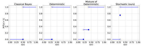
Figure 1: Examples of four different approaches to thresholding the regression function. Classical Bayes thresholding (Eq. (1)) always thresholds deterministically at $\eta(x)=0.5$ to optimize accuracy. Koyejo et al. (2014); Narasimhan et al. (2014) and others have suggested using other Deterministic thresholds (e.g., $\eta(x)=0.3$, shown here) to optimize other CMMs, assuming $\eta(X)$ is absolutely continuous. Wang et al. (2019a) showed that the optimal classifier can always be written as a Mixture of Deterministic (MD) classifiers (e.g., a $(0.3,0.7)$-mixture of thresholds at $\eta(x)=0.2$ and $\eta(x)=0.4$, shown here). Finally, we propose using a single Stochastic threshold (e.g., $(t,p)=(0.3,0.75)$, shown here). Only MD and Stochastic approaches are optimal in general (for arbitrary CMMs, without $\eta(X)$ absolutely continuous), while Stochastic thresholding is strictly simpler than MD.

The generality of Theorem 3 necessitates a significantly more complex proof than prior work. In particular, we prove Theorem 3 in Appendix A using a series of variational arguments. Roughly speaking, given a classifier $\widehat{Y}$, we construct a perturbation $\widehat{Y}^{\prime}$ of $\widehat{Y}$ such that either $M(C_{\widehat{Y}})<M(C_{\widehat{Y}^{\prime}})$ or $\widehat{Y}^{\prime}$ is an RTC and $M(C_{\widehat{Y}})\leq M(C_{\widehat{Y}^{\prime}})$. Since, the classifier $\widehat{Y}$ might be quite poorly behaved (e.g., its behavior on sets of $P_{X}$-measure $0$ could be arbitrary), the technical complexity lies in constructing admissible perturbations (i.e., those that are well-defined classifiers). For this reason, the proof of Theorem 3 involves a series of constructions of increasingly well-behaved classifiers.

Theorem 3 tells us that a generalized Bayes classifier can always be written in terms of the regression function $\eta$ and two scalar parameters $(t,p)$ depending on the distribution of $\eta(X)$ and the CMM $M$. The next example shows that this characterization cannot be simplified without stronger assumptions:

Example 4.

Suppose $\mathcal{X}=\{0\}$ is a singleton, $\eta(0)\in(0,1)$, and, for some $\theta>0$, $M(C)=(\text{TP})^{\theta}\text{TN}$. One can check that $M$ is a valid CMM. Suppose $\widehat{Y}$ is an RTC. It is straightforward to compute that $M(C_{\widehat{Y}})=(p\eta(0))^{\theta}(1-p)(1-\eta(0))1\{t=\eta(0)\}$, and that $M(C_{\widehat{Y}})$ is uniquely maximized by $p=\frac{\theta}{\theta+1}\in(0,1)$ and $t=\eta(0)\in(0,1)$. This shows that both threshold parameters $p$ and $t$ in an RTC are necessary, in the absence of further assumptions on $M$ or $\eta$. This example also illustrates the need for stochasticity to optimize general CMMs. Specifically, for any deterministic classifier $\widehat{Y}$, either $\widehat{Y}(0)=0$ (so $\text{TP}=0$) or $\widehat{Y}(0)=1$ (so $\text{TN}=0$); in either case, $M(C_{\widehat{Y}})=0$.

This performance gap between stochastic and deterministic classifiers is closely related to Theorem 1 of Cotter et al. (2019b), which provides a closely related lower bound on how well a stochastic classifier can be approximated by a deterministic one, in terms of the probability assigned to atoms of $\eta(X)$. However, Cotter et al. (2019b) only study how well stochastic classifiers can be approximated by deterministic ones (with the motivation of derandomizing classifiers), not whether stochastic classifiers can systematically outperform deterministic ones, as we show here.

4.3 Relative Performance Guarantees in terms of the Generalized Bayes Classifier

Theorem 3 motivates a two-step approach to imbalanced classification in which one first estimates the regression function $\eta$ and then selects a stochastic threshold $(t,p)$ that optimizes empirical performance $M(\widehat{C}_{\widehat{Y}})$. Such an approach has many practical advantages. For example, as we show in Appendix D, a simple algorithm can exactly optimize the threshold $(t,p)$ over large datasets in $O(n\log n)$ time. Additionally, one can address covariate shift or retune a classifier trained under one CMM to perform well under another CMM, simply by re-optimizing $(t,p)$, which is statistically and computationally much easier than retraining a classifier from scratch. In this section, we focus on an advantage for theoretical analysis, namely that the error of such a classifier decomposes into errors in selecting $(t,p)$ and errors in estimating $\eta$, allowing the derivation of performance guarantees relative a generalized Bayes classifier. All results in this section are proven in Appendix B.

We first bound the performance difference of thresholding two regressors in terms of their $\mathcal{L}_{\infty}$ distance. This will allow us to bound error due to using a regressor $\widehat{\eta}$ instead of the true $\eta$.

Lemma 5.

For $p,t\in[0,1]$, $\eta,\eta^{\prime}:\mathcal{X}\to[0,1]$, $\left\|C_{\widehat{Y}_{p,t,\eta}}-C_{\widehat{Y}_{p,t,\eta^{\prime}}}\right\|_{\infty}\leq\mathbb{P}\left[|\eta(X)-t|\leq\left\|\eta-\eta^{\prime}\right\|_{\infty}\right]$.

Intuitively, Lemma 5 bounds the largest difference in the confusion matrices of $\widehat{Y}_{p,t,\eta}$ and $\widehat{Y}_{p,t,\eta^{\prime}}$ by the probability that the threshold $t$ lies between $\eta$ and $\eta^{\prime}$. As we will show later, under a margin assumption, this can be bounded by the $\mathcal{L}_{\infty}$ distance between $\eta$ and $\eta^{\prime}$.

Our next lemma bounds the worst-case error over thresholds $(t,p)\in[0,1]$ of the empirical confusion matrix. This allows us to bound error due to using an empirical threshold $(\widehat{t},\widehat{p})$ instead of the threshold $(t^{*},p^{*})$ that is optimal for the true regression function.

Lemma 6.

Let $\eta:\mathcal{X}\to[0,1]$ be any regression function. Then, with probability at least $1-\delta$,

$$\sup_{p,t\in[0,1]}\left\|\widehat{C}_{\widehat{Y}_{p,t,\eta}}-C_{\widehat{Y}_{p,t,\eta}}\right\|_{\infty}\leq\sqrt{\frac{8}{n}\log\frac{32(2n+1)}{\delta}}.$$

Lemma 6 follows from Vapnik-Chervonenkis (VC) bounds on the complexity of the set $\{\widehat{Y}_{p,t,\eta}:p,t\in[0,1]\}$ of possible RTCs with fixed regression function $\eta$. In fact, Appendix B proves a more general bound on the error between empirical and true confusion matrices uniformly over any family $\mathcal{F}$ of stochastic classifiers in terms of the growth function of $\mathcal{F}$. Consequently, when $\mathcal{F}$ has finite VC dimension, we obtain uniform convergence at the fast rate $\sqrt{\log(n/\delta)/n}$. As we formalize later, this suggests that the difficulty in tuning an imbalanced classifier to optimize a CMM $M$ comes not from difficulty in estimating the confusion matrix but rather from the sensitivity of commonly used CMMs to the selected threshold. Because Theorem 3 shows that any CMM can be optimized by a RTC, we state here only the specific result for RTCs.

Before combining Lemmas 5 and 6 to give the main result of this section, we note a margin assumption, which characterizes separation between the two classes:

Definition 7 (Tsybakov Margin Condition).

Let $C,\beta\geq 0$, $t\in(0,1)$. A classification problem with covariate distribution $P_{X}$ and regression function $\eta$ satisfies a $(C,\beta)$-margin condition around $t$ if, for any $\epsilon>0$, $\mathbb{P}\left[|\eta(X)-t|\leq\epsilon\right]\leq C\epsilon^{\beta}$.

The Tsybakov margin condition, introduced by Mammen and Tsybakov (1999) for $t=0.5$, is widely used to establish convergence rates for classification in terms of accuracy (Audibert and Tsybakov, 2007; Arlot and Bartlett, 2011; Chaudhuri and Dasgupta, 2014). Together with the margin condition and a Lipschitz condition on the $M$, Lemmas 5 and 6 give the following bound on sub-optimality of an RTC if the threshold is selected by maximizing $M$ over the empirical confusion matrix:

Corollary 8.

Let $\eta:\mathcal{X}\to[0,1]$ be the true regression function and $\widehat{\eta}:\mathcal{X}\to[0,1]$ be any regressor.

$$\text{ Let }\quad\left(\widehat{p},\widehat{t}\right):=\operatornamewithlimits{\arg\!\max}_{(t,p)\in[0,1]^{2}}M\left(\widehat{C}_{\widehat{Y}_{p,t,\widehat{\eta}}}\right)\quad\text{and}\quad\left(p^{*},t^{*}\right):=\operatornamewithlimits{\arg\!\max}_{(t,p)\in[0,1]^{2}}M\left(C_{\widehat{Y}_{p,t,\eta}}\right)$$

denote the empirical and true optimal thresholds, respectively. Suppose $M$ is Lipschitz continuous with constant $L_{M}$ with respect to the uniform ($\mathcal{L}_{\infty}$) metric on $\mathcal{C}$. Finally, suppose $P_{X}$ and $\eta$ satisfy a $(C,\beta)$-margin condition around $t^{*}$. Then, with probability $\geq 1-\delta$,

$$M\left(C_{\widehat{Y}_{p^{*},t^{*},\eta}}\right)-M\left(C_{\widehat{Y}_{\widehat{p},\widehat{t},\widehat{\eta}}}\right)\leq L_{M}\left(C\left\|\eta-\widehat{\eta}\right\|_{\infty}^{\beta}+2\sqrt{\frac{8}{n}\log\frac{32(2n+1)}{\delta}}\right).$$

5 Uniform Error of the $k$NN Regressor

In the previous section, we bounded relative performance of an RTC in terms of uniform ($\mathcal{L}_{\infty}$) loss of the regression function estimate. Here, we bound uniform loss of one such regressor, the widely used $k$-nearest neighbor ($k$NN) regressor. Our analyses include a parameter $r$, introduced in Section 9, that characterizes a novel sub-type of class imbalance, which we call Uniform Class Imbalance. This leads to insights about how the behavior of the $k$NN classifier depends not only on the degree, but also on the structure, of class imbalance in a given dataset. We begin with some notation:

Definition 9 ($k$-Nearest Neighbor Regressor).

Given a point $x\in\mathcal{X}$, let $\sigma(x)$ denote a permutation of $\{1,...,n\}$ such that $X_{\sigma_{i}(x)}$ is the $i^{th}$-nearest neighbor of $x$ among $X_{1},...,X_{n}$. For integers $k\in[1,n]$, the $k$NN regressor $\widehat{\eta}_{k}:\mathcal{X}\to[0,1]$ is defined as

$$\widehat{\eta}_{k}(x)=\frac{1}{k}\sum_{i=1}^{k}Y_{\sigma_{i}(x)},\quad\text{ for all }x\in\mathcal{X}.$$ (4)

We now formalize a novel sub-type of class imbalance:

Definition 10 (Uniform Class Imbalance (UCI)).

Write the regression function as $\eta=r\zeta$, where $r\in(0,1]$ and $\zeta:\mathcal{X}\to[0,1]$ is a regression function with $\sup_{x\in\mathcal{X}}\zeta(x)=1$. A classification problem has Uniform Class Imbalance (UCI) in the number of samples $n$ if $r\to 0$ as $n\to\infty$.

Intuitively, in UCI, the class $Y=1$ is rare regardless of $X$. This includes “difficult” classification problems where the covariate $X$ provides only partial information about the class $Y$ and examples from the rare class lie deep within the distribution of the common class. Examples include rare disease diagnosis (Schaefer et al., 2020) or fraud detection (Awoyemi et al., 2017). In practice, the classifier’s role is often to flag “high-risk” samples $X$, those with $\eta(X)$ relatively high, for follow-up investigation. UCI can be distinguished from “easier” problems in which, for some $x\in\mathcal{X}$, $\eta(X)\approx 1$ and so, given enough training data, a classifier can confidently assign the label $Y=1$. These include well-separated classes or deterministic problems (e.g., protein structure prediction; Noé et al. (2020)).

To our knowledge, such notions of class imbalance have not previously been distinguished. In the particular case of data drawn from a logistic model, UCI reduces to the notion of class imbalance described in Wang (2020); however, UCI applies in more general contexts.

5.1 Uniform Risk Bounds

We now present bounds (proven in Appendix C.1) on uniform error $\left\|\eta-\widehat{\eta}\right\|_{\infty}=\sup_{x\in\mathcal{X}}|\eta(x)-\widehat{\eta}(x)|$ of the $k$NN regressor $\widehat{\eta}_{k}$. First, recall two standard quantities, covering numbers and shattering coefficients, by which we measure complexity of the feature space:

Definition 11 (Covering Number).

Suppose $(\mathcal{X},\rho)$ is a totally bounded metric space. Then, for any $\epsilon>0$, the $\epsilon$-covering number $N(\epsilon)$ of $(\mathcal{X},\rho)$ is the smallest integer such that there exist $N(\epsilon)$ points $x_{1},...,x_{N(\epsilon)}\in X$ satisfying $\mathcal{X}\subseteq\bigcup_{i=1}^{N(\epsilon)}B(x_{i},\epsilon)$.

Definition 12 (Shattering Coefficient).

For integers $n>0$, the shattering coefficient of balls in $(\mathcal{X},\rho)$ is $\displaystyle S(n)=\sup_{x_{1},...,x_{n}\in\mathcal{X}}\left|\left\{\{x_{1},...,x_{n}\}\cap B(x,\epsilon):x\in\mathcal{X},\epsilon\geq 0\right\}\right|$.

We now state two assumptions data distribution $P_{X,Y}$:

Assumption 13 (Dense Covariates Assumption).

For some $p_{*},\epsilon^{*},d>0$, the marginal distribution $P_{X}$ of covariates is lower bounded, for any $x\in\mathcal{X}$ and $\epsilon\in(0,\epsilon^{*}]$, by $P_{X}(B_{\epsilon}(x))\geq p_{*}\epsilon^{d}$.

Assumption 13 ensures that each query point’s nearest neighbors are sufficiently near to be informative. We also assume that the regression function $\zeta$ is smooth:

Assumption 14 (Hölder Continuity).

For some $\alpha\in(0,1]$, $L:=\sup_{x\neq x^{\prime}\in\mathcal{X}}\frac{\left|\zeta(x)-\zeta(x^{\prime})\right|}{\rho^{\alpha}(x,x^{\prime})}<\infty$.

We now state our upper bound on uniform error:

Theorem 15.

Under Assumptions 13 and 14, whenever $k/n\leq p_{*}(\epsilon^{*})^{d}/2$, for any $\delta>0$, with probability at least $1-N\left(\left(2k/(p_{*}n)\right)^{1/d}\right)e^{-k/4}-\delta$, we have

$$\left\|\eta-\widehat{\eta}\right\|_{\infty}\leq 2^{\alpha}Lr\left(\frac{2k}{p_{*}n}\right)^{\alpha/d}+\frac{2}{3k}\log\frac{2S(n)}{\delta}+\sqrt{\frac{2r}{k}\log\frac{2S(n)}{\delta}}.$$ (5)

If $r\in O\left((\log S(n)/n\right)$, this bound is minimized by $k\asymp n$, giving $\left\|\eta-\widehat{\eta}\right\|_{\infty}\in O_{P}\left((\log S(n))/n\right)$. Otherwise, this bound is minimized by $k\asymp n^{\frac{2\alpha}{2\alpha+d}}(\log S(n))^{\frac{d}{2\alpha+d}}r^{-\frac{d}{2\alpha+d}}$, giving

$$\left\|\eta-\widehat{\eta}\right\|_{\infty}\in O_{P}\left(\left((\log S(n))/n\right)^{\frac{\alpha}{2\alpha+d}}r^{\frac{\alpha+d}{2\alpha+d}}\right).$$

Of the three terms in (5), the first term, of order $r(k/n)^{\alpha/d}$, comes from smoothing bias of the $k$NN classifier. The second and third terms are due to label noise, with the second term dominating under extreme class imbalance $r\in O\left(\log S(n)/n\right)$ and the third term dominating otherwise. Theorem 5 shows that, under UCI, one should use a much larger choice of the tuning parameter $k$ than in the case of balanced classes; indeed, setting $k\asymp n^{\frac{2\alpha}{2\alpha+d}}(\log S(n))^{\frac{d}{2\alpha+d}}$, which is optimal in the balanced case, gives a rate that is suboptimal by a factor of $r^{-d/(4\alpha+d)}$.

The following example demonstrates how to apply Theorem 15 in a concrete setting of interest:

Corollary 16 (Euclidean, Absolutely Continuous Case).

Suppose $(\mathcal{X},\rho)=([0,1]^{d},\|\cdot\|_{2})$ is the unit cube in $\mathbb{R}^{d}$, equipped with the Euclidean metric, and $P_{X}$ has a density that is lower bounded away from $0$ on $\mathcal{X}$. Then, for $k\asymp n^{\frac{2\alpha}{2\alpha+d}}(\log n)^{\frac{d}{2\alpha+d}}r^{-\frac{d}{2\alpha+d}}$, $\left\|\eta-\widehat{\eta}\right\|_{\infty}\in O_{P}\left(\left((\log n)/n\right)^{\frac{\alpha}{2\alpha+d}}r^{\frac{\alpha+d}{2\alpha+d}}\right)$.

The most problematic term in this bound is the exponential dependence on the dimension $d$ of the covariates. Fortunately, since Theorem 15 utilizes covering numbers, it improves if the covariates exhibit structure, such as that of a low-dimensional manifold. We illustrate this in detail in Appendix C.1.

We close with a minimax lower bound, proven in Appendix C.2, on the uniform error of any estimator, over $(\alpha,L)$-Hölder regression functions. Up to a polylogarithmic factor in $r$, the rate of this lower bound matches that in Theorem 15, suggesting that both bounds are quite tight.

Theorem 17.

Suppose $\mathcal{X}=[0,1]^{d}$ is the $d$-dimensional unit cube and $X\sim\operatorname{Uniform}(\mathcal{X})$. Let $\Sigma^{\alpha}(L)$ denote the family of $(\alpha,L)$-Hölder continuous regression function. Then, there exist constants $n_{0}$ and $c>0$ (depending only on $\alpha$, $L$, and $d$) such that, for all $n\geq n_{0}$ and any estimator $\widehat{\eta}$,

$$\sup_{\zeta\in\Sigma^{\alpha}(L)}\mathop{\mathbb{P}}\left[\left\|\eta-\widehat{\eta}\right\|_{\infty}\geq c\left(\frac{\log(nr)}{n}\right)^{\frac{\alpha}{2\alpha+d}}r^{\frac{\alpha+d}{2\alpha+d}}\right]\geq\frac{1}{8}.$$

Discussion

Plugging the above upper bounds on $\left\|\eta-\widehat{\eta}\right\|_{\infty}$ into Corollary 8 provides error bound under arbitrary CMMs, in terms of the sample size $n$, hyperparameter $k$, UCI degree $r$, and complexity parameters (margin $\beta$, smoothness $\alpha$, intrinsic dimension $d$, etc.) of $\mathcal{X}$ and $P_{X,Y}$. Thus, these results collectively give some of the first complete finite-sample guarantees under general performance metrics used for imbalanced classification. Our analysis shows that, under severe UCI, the optimal $k$ is much larger than in balanced classification, whereas this same $k$ leads to sub-optimal, or even inconsistent, estimates of the regression function under other (nonuniform) forms of class imbalance.

6 Numerical Experiments

We provide two numerical experiments to illustrate our results from Sections 4 and 5. We repeat each experiment $100$ times and present average results with $95\%$ confidence intervals computed using the central limit theorem. Python implementations and instructions for reproducing each experiment can be found at https://gitlab.tuebingen.mpg.de/shashank/imbalanced-binary-classification-experiments. Further technical details regarding the experiments can be found in Appendix E, while Appendix F explores some predictions of our theoretical results on real data from a credit card fraud detection problem.

Experiment 1

Example 4 showed that, under general CMMs, deterministic RTCs are sometimes unable to approach optimal classification performance, necessitating stochastic RTCs. This experiment demonstrates this gap numerically. Suppose $\mathcal{X}=[0,1]$, over which $X$ is uniformly distributed, and for all $x\in\mathcal{X}$, $\eta(x)=0.5\cdot 1\{1/3\leq x<2/3\}+1\{2/3\leq x\}$.

Consider the CMM $M(C)=\text{TP}\cdot\text{TN}$. Similar to the analysis in Example 4, the optimal value of $M(C)=(5/12)^{2}=\frac{25}{144}$ is achievable only by a stochastic classifier, whereas as deterministic classifiers achieve at most $M(C)=1/6<25/144$.

For $10$ logarithmically spaced values of $n$ between $10^{2}$ and $10^{4}$, we drew $n$ independent samples of $(X,Y)$ according the above distribution. Using this training data, we selected optimal deterministic and stochastic thresholds $t\in[0,1]$ and $(t,p)\in[0,1]^{2}$ for the $k$NN classifier by maximizing $M(\widehat{C})$ over $10^{4}$ uniformly spaced values in $[0,1]$ and $[0,1]^{2}$, respectively. Since, in this example, $\alpha=d=1$, we set $k=\lfloor n^{2/3}\rfloor$ as suggested by Theorem 16. As another point of comparison, we also include a very different deterministic classifier, a random forest, trained with default parameters of Python’s scikit-learn package. We estimated $M(C)$ using $1000$ more independently generated test samples of $(X,Y)$. Figure 2(a) shows regret, i.e., sub-optimality of each classifier relative to the optimal classifier, in terms of $M(C)$. Consistent with our analysis, regrets of the deterministic classifiers are bounded away from $0$, while regret of the stochastic classifier vanishes as $n$ increases.

Experiment 2

This experiment demonstrates that making classifiers robust to severe class imbalance requires distinguishing different sub-types of class imbalance, such as UCI. Suppose $\mathcal{X}=[0,1]$, $X\sim\operatorname{Uniform}([0,1])$, and $r\in(0,1)$. Consider two regression functions $\eta_{1}(x)=r(1-x)$ and $\eta_{2}(x)=\max\{0,1-x/r\}$. $\eta_{1}$ and $\eta_{2}$ exhibit the same overall class imbalance, with $r/2$ proportion of samples from class $1$. The regression function $\eta_{1}$ satisfies UCI of degree $r$, whereas $\eta_{2}$ does not satisfy a nontrivial degree of UCI. For sufficiently small $r\in(0,1)$, specifically $r\in o\left(n^{-d/(2\alpha+2d)}\right)$, Theorem 15 gives that the optimal choice of $k$ under $\eta_{1}$ satisfies $k\in\omega(rn)$. On the other hand, if $k\in\omega(rn)$, then, under $\eta_{2}$, $\operatornamewithlimits{\mathbb{E}}\left[\widehat{\eta}_{k}(0)\right]\to 0$, so that $\widehat{\eta}_{k}(0)$ is an inconsistent estimate of $\eta_{2}(0)=1$.

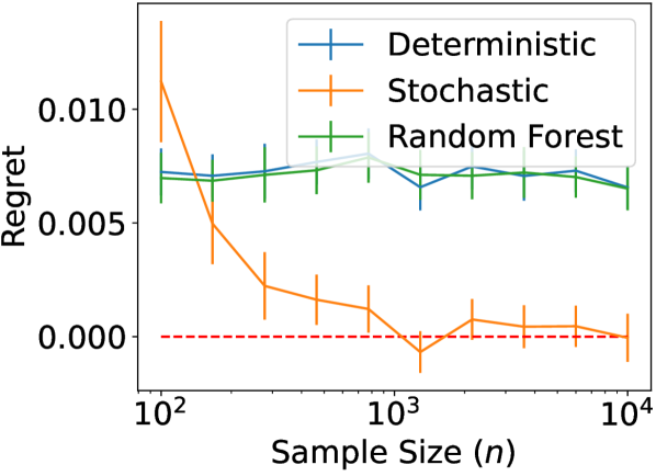
(a) Experiment 1

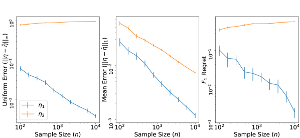
(b) Experiment 2

Figure 2: (a) Regret of deterministically and stochastically thresholding the $k$NN classifier, under the CMM $M(C)=\text{TP}\cdot\text{TN}$. (b) Uniform ($\mathcal{L}_{\infty}$) and average ($\mathcal{L}_{1}$) errors of $k$NN regressor, as well as $F_{1}$ regret of estimating regression functions $\eta_{1}$ and $\eta_{2}$. Error bars indicate $95\%$ confidence intervals.

For $10$ logarithmically spaced values of $n$ between $10^{2}$ and $10^{4}$, we drew $n$ independent samples of $(X,Y)$ according the joint distributions corresponding to each of $\eta_{1}$ and $\eta_{2}$. Since, in this example, $\alpha=d=1$, to ensure $r\in o\left(n^{-d/(2\alpha+2d)}\right)$, we set $r=n^{-1/2}$. As indicated by Corollary 16, we set $k=\lfloor n^{2/3}r^{-1/3}\rfloor$. We then computed $\mathcal{L}_{\infty}$ and $\mathcal{L}_{1}$ distances between the $k$NN regressor (Eq. (4)) and true regression function. We also drew $1000$ independent test samples of $(X,Y)$ and used these to estimate the $F_{1}$ score of thresholding the $k$NN regressor at a threshold $t$ determined by optimizing the empirical $F_{1}$ score (over the training data) over $100$ uniformly-spaced values of $t\in[0,1]$. Figure 2(b) shows the uniform ($\mathcal{L}_{\infty}$) error, the average ($\mathcal{L}_{1}$) error, and the $F_{1}$ regret, which we bounded in Corollary 8. Consistent with our analysis above, the uniform ($\mathcal{L}_{\infty}$) error decays to $0$ under $\eta_{1}$ but not under $\eta_{2}$. Meanwhile, the average error ($\mathcal{L}_{1}$) decays to $0$ under both $\eta_{1}$ and $\eta_{2}$. Consistent with Corollary 8, the $F_{1}$ regret of the thresholded classifier, which decays to $0$ under $\eta_{1}$ but not under $\eta_{2}$, mirrors performance of the regressor in uniform ($\mathcal{L}_{\infty}$) error rather than average ($\mathcal{L}_{1}$) error.

7 Conclusions

Our main conclusions are as follows. First, without any assumptions on the data-generating distribution, the Bayes-optimal classifier generalizes from accuracy to other performance metrics using a stochastic thresholding procedure, while, in general, deterministic classifiers may not achieve Bayes-optimality. This generalized Bayes classifier provides an optimal performance benchmark relative to which one can analyze classifiers that threshold estimates of the regression function. This includes the $k$NN classifier, for which we provided new guarantees, including minimax-optimally under uniform loss in the presence of Uniform Class Imbalance. Our results imply that the parameter $k$ needs to be tuned differently for different sub-types of imbalanced classification, suggesting that developing reliable classifiers for severely imbalanced classes may require a more nuanced understanding of the data at hand. Further work is needed to (a) understand how sub-types of class imbalance can be distinguished in practice, (b) develop adaptive classifiers that perform well under multiple imbalance sub-types, and (c) extend our results to the multiclass case.

While this paper focused on statistical properties of stochastic classification, we should point out that using stochastic classifiers in real applications may require careful consideration of possible downstream consequences. On one hand, Theorem 3 provides justification for using (a limited degree of) stochasticity to break certain ties between classes: sometimes, this is provably necessary to optimize performance according to certain metrics. Stochastic classifiers can also be easier to train (Cotter et al., 2019a; Lu et al., 2020) or more robust to adversarial examples (Pinot et al., 2022). However, stochastic classifiers have risks, including being harder to interpret, explain, or debug, and being vulnerable to manipulation by downstream users (e.g., a user might query the classifier multiple times to produce a desired prediction). Stochastic classifiers may also violate certain notions of fairness, as individuals with identical features might be assigned to different classes. Techniques for derandomizing classifiers (Cotter et al., 2019b; Wu et al., 2022) may help address these issues.

Checklist

1. For all authors…

   1. Do the main claims made in the abstract and introduction accurately reflect the paper’s contributions and scope? [Yes]

   2. Did you describe the limitations of your work? [Yes]

   3. Did you discuss any potential negative societal impacts of your work? [N/A]

   4. Have you read the ethics review guidelines and ensured that your paper conforms to them? [Yes]

2. If you are including theoretical results…

   1. Did you state the full set of assumptions of all theoretical results? [Yes]

   2. Did you include complete proofs of all theoretical results? [Yes] See Appendices A, B, and C.

3. If you ran experiments…

   1. Did you include the code, data, and instructions needed to reproduce the main experimental results (either in the supplemental material or as a URL)? [Yes] Code and instructions for reproducing the experimental results are included in the supplemental material.

   2. Did you specify all the training details (e.g., data splits, hyperparameters, how they were chosen)? [Yes]

   3. Did you report error bars (e.g., with respect to the random seed after running experiments multiple times)? [Yes]

   4. Did you include the total amount of compute and the type of resources used (e.g., type of GPUs, internal cluster, or cloud provider)? [Yes] See Appendix E.

4. If you are using existing assets (e.g., code, data, models) or curating/releasing new assets…

   1. If your work uses existing assets, did you cite the creators? [Yes]

   2. Did you mention the license of the assets? [Yes]

   3. Did you include any new assets either in the supplemental material or as a URL? [N/A]

   4. Did you discuss whether and how consent was obtained from people whose data you’re using/curating? [N/A]

   5. Did you discuss whether the data you are using/curating contains personally identifiable information or offensive content? [N/A]

5. If you used crowdsourcing or conducted research with human subjects…

   1. Did you include the full text of instructions given to participants and screenshots, if applicable? [N/A]

   2. Did you describe any potential participant risks, with links to Institutional Review Board (IRB) approvals, if applicable? [N/A]

   3. Did you include the estimated hourly wage paid to participants and the total amount spent on participant compensation? [N/A]

Appendix A Derivation of the Generalized Bayes Classifier

In this Appendix, we prove Theorem 3, in which we characterize a stochastic generalization of the Bayes classifier to arbitrary CMMs. We reiterate the theorem for the reader here:

Theorem 3.

If $\operatornamewithlimits{\arg\!\max}_{\widehat{Y}\in\mathcal{SC}}M(C_{\widehat{Y}})\neq\varnothing$, then there exists a regression-thresholding classifier

$$\widehat{Y}_{p,t,\eta}\in\operatornamewithlimits{\arg\!\max}_{\widehat{Y}\in\mathcal{SC}}M(C_{\widehat{Y}}).$$

As described in the main paper, unlike prior results [Koyejo et al., 2014, Yan et al., 2018, Wang et al., 2019b], we do not assume that the distribution of $\eta(X)$ is absolutely continuous. This makes proving Theorem considerably more complicated than these previous results. We prove Theorem 3 in a sequence of steps, constructing optimal classifiers in forms progressively closer to that of the generalized Bayes classifier described in Theorem 3. Specifically, we first show, in Lemma 18, that there exists an optimal classifier that is a (stochastic) function of the true regression function $\eta^{*}$. We then construct an optimal classifier in which this function of $\eta^{*}$ is non-decreasing. Finally, we construct an optimal classifier in which this function of $\eta^{*}$ is a threshold function, as in Theorem 3.

Lemma 18.

For any stochastic classifier $\widehat{Y}:\mathcal{X}\to\mathcal{B}$, there is a stochastic classifier $\widehat{Y}^{\prime}:\mathcal{X}\to\mathcal{B}$ of the form

$$\widehat{Y}^{\prime}(x)\sim\text{Bernoulli}(f(\eta^{*}(x))),$$ (6)

for some $f:[0,1]\to[0,1]$, such that $C_{\widehat{Y}^{\prime}}=C_{\widehat{Y}}$.

Proof.

We start by defining the regression function and discussing formal probability notation. Let $\mathcal{F}=\sigma(\eta^{*}(Z))$ be the $\sigma$-field generated by the true regression function $\eta^{*}(Z)$. Define $\widehat{Y}^{\prime}:\mathcal{X}\to\mathcal{B}$ by

$$\widehat{Y}^{\prime}(x)\sim\text{Bernoulli}\left(\operatornamewithlimits{\mathbb{E}}_{Z\sim P_{X}}\left[\widehat{Y}(Z)\middle|\mathcal{F}\right](\eta^{*}(x))\right),$$

where by the $\eta^{*}(x)$ we are explicitly indicating that $\eta^{*}(x)$ is the input to the conditional expectation, as the conditional expectation is a measurable function of $\eta^{*}(Z)$. In the sequel, following standard conventions, we omit such notation. Note that $\widehat{Y}^{\prime}$ has the desired form and is defined almost surely.

Now, we get our final notes in place before proceeding with calculations. Let $\mathcal{G}=\sigma(X)$ be the $\sigma$-field generated by $X$.

A key step in the proof is showing the equality

$$\operatornamewithlimits{\mathbb{E}}\left[Y\widehat{Y}^{\prime}(X)\middle|\mathcal{F}\right] =\eta^{*}(X)\operatornamewithlimits{\mathbb{E}}\left[\widehat{Y}(X)\middle|\mathcal{F}\right]=\operatornamewithlimits{\mathbb{E}}\left[Y\widehat{Y}(X)\middle|\mathcal{F}\right].$$ (7)

We first provide an intuitive summary. Observe that conditioned on $\eta^{*}(X)$, $Y$ is independent of $\widehat{Y}$ and $\widehat{Y}^{\prime}$ separately. Thus, we can integrate over $Y$ and get the $\eta^{*}(X)$. By the definition of $\widehat{Y}^{\prime}$ we obtain the conditional expectation with respect to $Y$, and we have the resulting equality.

For the time being, taking Equation (7) as fact, we complete the rest of the proof. Combining Equation (7) and the tower property of conditional expectation, we have

$$\text{TP}_{\widehat{Y}^{\prime}} =\operatornamewithlimits{\mathbb{E}}\left[Y\widehat{Y}^{\prime}(X)\right]=\operatornamewithlimits{\mathbb{E}}\left[\operatornamewithlimits{\mathbb{E}}\left[Y\widehat{Y}^{\prime}(X)\middle|\mathcal{F}\right]\right]=\operatornamewithlimits{\mathbb{E}}\left[\operatornamewithlimits{\mathbb{E}}\left[Y\widehat{Y}(X)\middle|\mathcal{F}\right]\right]=\operatornamewithlimits{\mathbb{E}}\left[Y\widehat{Y}(X)\right]=\text{TP}_{\widehat{Y}}.$$

Similarly, one can check that $C_{\widehat{Y}^{\prime}}=C_{\widehat{Y}}$. ∎

Proof of Equation (7).

We now present the formal details to establish Equation (7), which may be skipped if one is uninterested in the measure-theoretic details. We first to set up the random variables needed to formalize the above intuition. Let $S$, $T$, $U$, $V$, and $W$ be random variables. Let $(S,T)=(\eta^{*}(X),X)$. We also require $U$ and $V$ to be uniform on $[0,1]$. We need not specify the precise distribution $W$. Further, let $(S,T)$, $U$, $V$, and $W$ all be independent. For notation purposes, it is convenient for the underlying probability space $(\Omega,\mathcal{G},\mathbb{P})$ to be the product probability space of some probability spaces to the extent possible. In particular, we require the set $\Omega=\bigtimes_{i=S}^{W}\Omega_{i}$ and a set $B$ in $\mathcal{G}$ to have a product structure $B=\bigtimes_{i=S}^{W}B_{i}$ for ease of exposition. Note that the measure $\mathbb{P}$ is not a product measure, as $S$ and $T$ are dependent, although it is a product measure with respect to the laws of $(S,T)$, $U$, $V$, $W$.

Now, we define $Y$, $\widehat{Y}^{\prime}$, and $\widehat{Y}$ in terms of $U$, $V$, $W$, and $X$. Define

$$Y(\eta^{*}(X)) =\mathbf{1}\{U\leq\eta^{*}(X)\}$$

$$\widehat{Y}^{\prime}(\eta^{*}(X)) =\mathbf{1}\{V\leq\operatornamewithlimits{\mathbb{E}}[\widehat{Y}|\mathcal{F}]\}$$

$$\widehat{Y}(X) =r(S,T,W),$$

where here $U$ serves as the noise in $Y$, $V$ serves as the internal randomization of $\widehat{Y}^{\prime}$, and $W$ serves as the possible internal randomization of $\widehat{Y}$. Here, $\mathbf{1}$ is the indicator taking the value 1 if the event in curly braces occurs and 0 otherwise, and $r$ is some function. Note that this is still of the desired form.

To prove the first part of Equation (7), i.e., to show that the middle term $M=\eta^{*}(X)\operatornamewithlimits{\mathbb{E}}[\widehat{Y}(X)|\mathcal{F}]=S\operatornamewithlimits{\mathbb{E}}[\widehat{Y}|\mathcal{F}]$ is indeed the conditional expectation of the left of Equation (7), we must verify two conditions: (i) $M$ is $\mathcal{F}$-measurable and (ii) the integrals of $Y\widehat{Y}^{\prime}$ and $M$ are identical on any event $A$ in $\mathcal{F}$ [Durrett, 2010, page 221]. Condition (i) is immediate, since $M$ is a function of $\eta^{*}(X)$ and nothing more.

For condition (ii), we do a bit of computation. Let $A=A_{S}\times A_{T}\times A_{U}\times A_{V}\times A_{W}$ be an event in $\mathcal{F}$. Note that because $A$ is $\mathcal{F}$-measurable, the sets $A_{U}$ and $A_{V}$ must be all of $\Omega_{U}$ and $\Omega_{V}$ or the empty set. Suppose for the moment that both are non-empty. Then, we have

$$\int_{A}Y\widehat{Y}^{\prime}d\mathbb{P} =\int_{A_{S}}\int_{A_{V}}\int_{A_{U}}\mathbf{1}\left\{U\leq S\right\}\mathbf{1}\{V\leq\operatornamewithlimits{\mathbb{E}}[\widehat{Y}|\mathcal{F}]\}d\mathbb{P}_{U}d\mathbb{P}_{V}d\mathbb{P}_{S}$$

$$=\int_{A_{S}}\int_{A_{V}}S\mathbf{1}\{V\leq\operatornamewithlimits{\mathbb{E}}[\widehat{Y}|\mathcal{F}]\}d\mathbb{P}_{V}d\mathbb{P}_{S}$$

$$=\int_{A_{S}}S\operatornamewithlimits{\mathbb{E}}[\widehat{Y}|\mathcal{F}]d\mathbb{P}_{S}$$

$$=\int_{A}S\operatornamewithlimits{\mathbb{E}}[\widehat{Y}|\mathcal{F}]d\mathbb{P}.$$

Note that the crucial first and last equalities in which we break and reform the integral over the entire event in terms of its coordinates is possible due to Fubini’s theorem for integrable functions. This proves the desired equality when $A_{U}=\Omega_{U}$ and $A_{V}=\Omega_{V}$, and from the preceding calculation we can see that the integrals are both 0 when either $A_{U}=\emptyset$ or $A_{V}=\emptyset$, and so the desired equality holds. This establishes the left equality of Equation (7).

Establishing the right hand side of Equation (7) also takes a bit of calculation. First, we have already verified the measurability condition (i), and so all that remains is to check the integral equality. Again, let $A$ be an event in $\mathcal{F}$, and assume that $A_{T}$, $A_{U}$, and $A_{W}$ are non-empty. We have

$$\int_{A}Y\widehat{Y}d\mathbb{P} =\int_{A_{S}}\int_{A_{T}}\int_{A_{W}}\int_{A_{U}}\mathbf{1}\left\{U\leq S\right\}r(S,T,W)d\mathbb{P}_{U}d\mathbb{P}_{W}d\mathbb{P}_{T}d\mathbb{P}_{S}$$

$$=\int_{A_{S}}\int_{A_{T}}\int_{A_{W}}S\;r(S,T,W)d\mathbb{P}_{W}d\mathbb{P}_{T}d\mathbb{P}_{S}$$

$$=\int_{A_{S}}S\left(\int_{A_{T}}\int_{A_{W}}r(S,T,W)d\mathbb{P}_{W}d\mathbb{P}_{T}\right)d\mathbb{P}_{S}.$$

Note that Fubini’s theorem is again used in the first step. In the event that any of $A_{T}$, $A_{U}$, or $A_{W}$ is empty, then the above equation is 0 and equality holds. Now, we have to show that the random variable $M^{\prime}=\int_{A_{T}}\int_{A_{W}}r(S,T,W)d\mathbb{P}_{W}d\mathbb{P}_{T|S}$ is the conditional expectation of $\widehat{Y}$ with respect to $\mathcal{F}$. Measurability is readily apparent, as $M^{\prime}$ is a function of $S$ and no more. Now, we check the condition that $\widehat{Y}$ and $M^{\prime}$ have the same integral on an event $A$ in $\mathcal{F}$. Again assume that $A_{U}$ and $A_{W}$ are non-empty, observing in the calculation to follow that equality holds with the value 0 if either is empty. Using Fubini’s theorem and some direct computation, we have

$$\int_{A}\widehat{Y}d\mathbb{P} =\int_{A}r(S,T,W)d\mathbb{P}$$

$$=\int_{A_{S}}\int_{A_{T}}\int_{A_{W}}r(S,T,W)d\mathbb{P}_{W}d\mathbb{P}_{T}d\mathbb{P}_{S}$$

$$=\int_{A}\left(\int_{A_{T}}\int_{A_{W}}r(S,T,W)d\mathbb{P}_{W}d\mathbb{P}_{T}\right)d\mathbb{P}$$

$$=\int_{A}M^{\prime}d\mathbb{P}.$$

This completes the proof that the conditional expectation of $\widehat{Y}$ is $M^{\prime}$, and so it proves that the conditional expectation of $Y\widehat{Y}$ is $\eta^{*}(X)\operatornamewithlimits{\mathbb{E}}[\widehat{Y}|\mathcal{F}].$ This is the right equality of Equation (7), thus completing the proof. ∎

It follows from Lemma 18 that, if $M(C_{\widehat{Y}})$ is maximized by any stochastic classifier, then it is maximized by a classifier $\widehat{Y}$ of the form in Eq. (6). It remains to show that $f$ in Eq. (6) can be of the form $z\mapsto p1\{z=t\}+1\{z>t\}$ for some threshold $(p,t)\in[0,1]^{2}$. Before proving this, we give a simplifying lemma showing that the problem of maximizing a CMM can be equivalently framed as a particular functional optimization problem. This will allow us to to significantly simplify the notation in the subsequent proofs.

Lemma 19.

Let $M$ be a CMM, and suppose that $M(C_{\widehat{Y}})$ is maximized (over $\mathcal{SC}$) by a classifier $\widehat{Y}$ of the form

$$\widehat{Y}(x)\sim\operatorname{Bernoulli}(f(\eta(x))),$$

for some $f^{*}:[0,1]\to[0,1]$. Let $f$ be a solution to the optimization problem

$$\max_{f:[0,1]\to[0,1]}\operatornamewithlimits{\mathbb{E}}[\eta(X)f(\eta(X))]\;\text{ s.t. }\;\operatornamewithlimits{\mathbb{E}}[(1-\eta(X))f(\eta(X))]\leq\operatornamewithlimits{\mathbb{E}}[(1-\eta(X))f^{*}(\eta(X))].$$ (8)

Then, the classifier

$$\widehat{Y}^{\prime}(x)\sim\operatorname{Bernoulli}(f(\eta(x))),$$

also maximizes $M(C_{\widehat{Y}^{\prime}})$ (over $\mathcal{SC}$).

Proof.

This result follows from the definition (Definition 1) of a CMM. Specifically, by construction of $\widehat{Y}^{\prime}$,

$$\text{TP}_{\widehat{Y}^{\prime}}=\operatornamewithlimits{\mathbb{E}}[\eta(X)f(\eta(X))]\geq\operatornamewithlimits{\mathbb{E}}[\eta(X)f^{*}(\eta(X))]=\text{TP}_{\widehat{Y}}$$

and

$$\text{FP}_{\widehat{Y}^{\prime}}=\operatornamewithlimits{\mathbb{E}}[(1-\eta(X))f(\eta(X))]\leq\operatornamewithlimits{\mathbb{E}}[(1-\eta(X))f^{*}(\eta(X))]=\text{FP}_{\widehat{Y}}.$$

Moreover, since the proportions of positive and negative true labels are independent of the chosen classifier (i.e., $\text{TP}_{\widehat{Y}^{\prime}}+\text{FN}_{\widehat{Y}^{\prime}}=\text{TP}_{\widehat{Y}}+\text{FN}_{\widehat{Y}}$ and $\text{FP}_{\widehat{Y}^{\prime}}+\text{TN}_{\widehat{Y}^{\prime}}=\text{FP}_{\widehat{Y}}+\text{TN}_{\widehat{Y}}$), we have

$$C_{\widehat{Y}^{\prime}}=\begin{bmatrix}\text{TN}_{\widehat{Y}}+\epsilon_{1}&\text{FP}_{\widehat{Y}}-\epsilon_{1}\\ \text{FN}_{\widehat{Y}}-\epsilon_{2}&\text{TP}_{\widehat{Y}}+\epsilon_{2},\end{bmatrix},$$

where $\epsilon_{1}:=\text{FP}_{\widehat{Y}}-\text{FP}_{\widehat{Y}^{\prime}}\in[0,\text{FP}_{\widehat{Y}}]$ and $\epsilon_{2}:=\text{TP}_{\widehat{Y}^{\prime}}-\text{TP}_{\widehat{Y}}\in[0,\text{FN}]$. Thus, by the definition (Definition 1) of a CMM, $M(C_{\widehat{Y}^{\prime}})\geq M(C_{\widehat{Y}})$. ∎

Lemma 19 essentially shows that maximizing any CMM $M$ is equivalent to performing Neyman-Pearson classification, at some particular false positive level $\alpha$ depending on $M$ (through $f^{*}$) and on the distribution of $\eta(X)$. For our purposes, this simplifies the remaining steps in proving Theorem 3 by allowing us to ignore the details of the particular CMM $M$ and regression function $\eta$ and focus on characterizing solutions to an optimization problem of the form (8) (see, specifically, (9) below).

To characterize solutions to this optimization problem, we will utilize the following two measure-theoretic technical lemmas:

Lemma 20.

Let $\mu$ be a measure on $[0,1]$ with $\mu([0,1])>0$. Then, there exists $z\in\mathbb{R}$ such that, for all $\epsilon>0$, $\mu([0,1]\cap(z-\epsilon,z))>0$.

Proof.

We prove the contrapositive. Suppose that, for every $z\in[0,1]$, there exists $\epsilon_{z}>0$ such that $\mu([0,1]\cap(z-\epsilon_{z},z))=0$. The family $\mathcal{S}:=\{[0,1]\cap(z-\epsilon_{z},z):z\in\mathbb{R}\}$ is an open cover of $[0,1]$. Since $[0,1]$ is compact, there exists a finite sub-cover $\mathcal{S}^{\prime}\subseteq\mathcal{S}$ of $[0,1]$. Thus, by countable subaddivity of measures,

$$\mu([0,1])\leq\sum_{S\in\mathcal{S}^{\prime}}\mu(\mathcal{S})=0.$$

∎

Lemma 21.

Let $(\mathcal{X},\Sigma,\mu)$ be a measure space, let $E,F\in\Sigma$ be measurable sets, and let $f:\mathcal{X}\to\mathbb{R}$ be a $\Sigma$-measurable function. If

$$\operatorname*{\text{ess~{}sup}}_{\mu}f(E)>\operatorname*{\text{ess~{}inf}}_{\mu}f(F),$$

then there exist measurable sets $A\subseteq E$ and $B\subseteq F$ with $\mu(A),\mu(B)>0$, and

$$\inf_{x\in A}f(x)>\sup_{x\in B}f(x).$$

Proof.

If $\operatorname*{\text{ess~{}sup}}_{\mu}f(E)>\operatorname*{\text{ess~{}inf}}_{\mu}f(F)$, then there exist $a>b$ such that $\operatorname*{\text{ess~{}sup}}_{\mu}f(E)>a>b>\operatorname*{\text{ess~{}inf}}_{\mu}f(F)$. Since $\operatorname*{\text{ess~{}sup}}_{\mu}f(E)>a$, it follows that $P_{Z}(E\cap\{z:f(z)\geq a\})>0$. Similarly, since $\operatorname*{\text{ess~{}inf}}_{\mu}f(F)<b$, it follows that $P_{Z}(F\cap\{z:f(z)\leq b\})>0$. Hence, letting $A=E\cap\{z:f(z)\geq a\}$ and $B=F\cap\{z:f(z)\leq b\}$, we have

$$\inf_{z\in A}f(z)\geq a>b\geq\sup_{z\in B}f(z).$$

∎

We are now ready for the main remaining step in the proof of Theorem 3, namely characterizing solutions of (a generalization of) the optimization problem (8):

Lemma 22.

Let $Z$ be a $[0,1]$-valued random variable, and let $c\in[0,1]$. Suppose that the optimization problem

$$\max_{f:[0,1]\to[0,1]\text{ measurable}}\operatornamewithlimits{\mathbb{E}}[Zf(Z)]\quad\text{ subject to }\quad\operatornamewithlimits{\mathbb{E}}[(1-Z)f(Z)]\leq c$$ (9)

has a solution. Then, there is a solution to (9) that is a stochastic threshold function.

Proof.

Suppose that there exists a solution $f$ to (9). We will construct a stochastic threshold function that solves (9) in two main steps. First, we will construct a monotone solution to (9). Second, we will show that this monotone solution is equal to a stochastic threshold function except perhaps on a set of probability $0$ with respect to $Z$. This stochastic threshold function is therefore a solution to (9).

Construction of Monotone Solution to (9): Define

$$g(z):=\operatorname*{\text{ess~{}sup}}_{P_{Z}}f([0,z])\quad\text{ and }\quad h(z):=\operatorname*{\text{ess~{}inf}}_{P_{Z}}f((z,1]),$$

where the essential supremum and infimum are taken with respect to the measure $P_{Z}$ of $Z$, with the conventions $g(z)=0$ whenever $P_{Z}([0,z])=0$ and $h(z)=1$ whenever $P_{Z}((z,1])=0$. We first show that, for all $z\in[0,1]$, $g(z)\leq h(z)$. We will then use this to show that $g=f$ except on a set of $P_{Z}$ measure $0$ (i.e., $P_{Z}(\{z\in[0,1]:g(z)\neq f(z)\})=0$). Therefore, both $\operatornamewithlimits{\mathbb{E}}[Zg(Z)]=\operatornamewithlimits{\mathbb{E}}[Zf(Z)]$ and $\operatornamewithlimits{\mathbb{E}}[(1-Z)g(Z)]=\operatornamewithlimits{\mathbb{E}}[(1-Z)f(Z)]$. Since $g:[0,1]\to[0,1]$ is clearly monotone non-decreasing, the result follows.

Suppose, for sake of contradiction, that, for some $z\in[0,1]$, $g(z)>h(z)$. By Lemma 21, there exist $A\subseteq[0,z]$ and $B\subseteq(z,1]$ such that $\inf_{z\in A}f(z)>\sup_{z\in B}f(z)$ and $P_{Z}(A),P_{Z}(B)>0$. Define $z_{A}:=\operatornamewithlimits{\mathbb{E}}[Z|Z\in A]$ and $z_{B}:=\operatornamewithlimits{\mathbb{E}}[Z|Z\in B]$, and note that, since $A\subseteq[0,z]$ and $B\subseteq(z,1]$, $z_{A}<z_{B}$. Define,

$$\epsilon:=\min\left\{\frac{P_{Z}(A)(1-z_{A})}{P_{Z}(B)(1-z_{B})}\inf_{z\in A}f(z),\quad 1-\sup_{z\in B}f(z)\right\}>0$$

and define $\phi:[0,1]\to[0,1]$ by

$$\phi(z):=\left\{\begin{array}[]{cc}f(z)-\epsilon\frac{P_{Z}(B)(1-z_{B})}{P_{Z}(A)(1-z_{A})}&\text{ if }z\in A\\ f(z)+\epsilon&\text{ if }z\in B\\ f(z)&\text{ otherwise,}\end{array}\right.$$

noting that, by construction of $\epsilon$, $\phi(z)\in[0,1]$ for all $z\in[0,1]$. Then, by construction of $\phi$,

$$\operatornamewithlimits{\mathbb{E}}[(1-Z)\phi(Z)]-\operatornamewithlimits{\mathbb{E}}[(1-Z)f(Z)] =-(1-z_{A})\epsilon\frac{P_{Z}(B)(1-z_{B})}{P_{Z}(A)(1-z_{A})}P_{Z}(A)+(1-z_{B})\epsilon P_{Z}(B)$$

$$=0\cdot\epsilon=0,$$

while

$$\operatornamewithlimits{\mathbb{E}}[Z\phi(Z)]-\operatornamewithlimits{\mathbb{E}}[Zf(Z)] =-z_{A}\epsilon\frac{P_{Z}(B)(1-z_{B})}{P_{Z}(A)(1-z_{A})}P_{Z}(A)+z_{B}\epsilon P_{Z}(B)$$

$$=\left(-\frac{z_{A}}{1-z_{A}}(1-z_{B})+z_{B}\right)\epsilon P_{Z}(B)>0,$$

since the function $z\mapsto\frac{z}{1-z}$ is strictly increasing. This contradicts the assumption that $f$ optimizes (9), implying $g\leq h$.

We now show that $g=f$ except on a set of $P_{Z}$ measure $0$. First, note that, if $g(z)\neq f(z)$, then $g(z)=\operatorname*{\text{ess~{}sup}}f([0,z])=\operatorname*{\text{ess~{}sup}}f([0,z))$, and so $g$ is left-continuous at $z$.

For any $\delta>0$, define

$$A_{\delta}:=\left\{z\in[0,1]:g(z)<f(z)-\delta\right\}\quad\text{ and }\quad B_{\delta}:=\left\{z\in[0,1]:g(z)>f(z)+\delta\right\}.$$

Since

$$\{z\in[0,1]:g(z)<f(z)\}=\bigcup_{j=1}^{\infty}\left\{z\in[0,1]:g(z)<f(z)-\frac{1}{j}\right\}$$

and

$$\{z\in[0,1]:g(z)>f(z)\}=\bigcup_{j=1}^{\infty}\left\{z\in[0,1]:g(z)>f(z)+\frac{1}{j}\right\},$$

by countable subadditivity, it suffices to show that $P_{Z}(A_{\delta})=P_{Z}(B_{\delta})=0$ for all $\delta>0$.

Suppose, for sake of contradiction, that $P_{Z}(A_{\delta})>0$. Applying Lemma 20 to the measure $E\mapsto P_{Z}(A_{\delta}\cap E)$, there exists $z\in\mathbb{R}$ such that, for any $\epsilon>0$, $P_{Z}(A_{\delta}\cap(z-\epsilon,z))>0$. Since $g$ is continuous at $z$, there exists $\epsilon>0$ such that $g(z-\epsilon)\geq g(z)-\delta$, so that, for all $z\in A_{\delta}\cap(z-\epsilon,z)$, $f(z)>g(z)+\delta$. Then, since $P_{Z}(A_{\delta}\cap(z-\epsilon,z))>0$, we have the contradiction

$$g(z)\geq\operatorname*{\text{ess~{}sup}}f(A_{\delta}\cap(z-\epsilon,z))>g(z).$$

On the other hand, suppose, for sake of contradiction, that $P_{Z}(B_{\delta})>0$. Applying Lemma 20 to the measure $E\mapsto P_{Z}(B_{\delta}\cap E)$, there exists $z\in\mathbb{R}$ such that, for any $\epsilon>0$, $P_{Z}(B_{\delta}\cap(z-\epsilon,z))>0$. Since $g$ is continuous at $z$, there exists $\epsilon>0$ such that $g(z-\epsilon)\geq g(z)-\delta$. At the same time, since $g$ is non-decreasing, for $t\in B_{\delta}\cap(z-\epsilon,z)$, $f(t)<g(t)-\delta\leq g(z)-\delta$. Thus, since $P_{Z}(B_{\delta}\cap(z-\epsilon,z))>0$, we have $h(z-\epsilon)<g(z)-\delta<g(z-\epsilon)$, contradicting the previously shown fact that $g\leq h$.

To conclude, we have shown that $P_{Z}(\{z\in[0,1]:g(z)\neq f(z)\})=0$.

Construction of a Stochastic Threshold Solution: We now construct a solution to (9) that is equal to a stochastic threshold function (i.e., a function that has the form $p1\{z=t\}+1\{z>t\}$) except on a set of $P_{Z}$-measure $0$. To show this, it suffices to construct a function $f:[0,1]\to[0,1]$ such that (a) $f$ is monotone non-decreasing and (b) the set $f^{-1}((0,1))$ is the union of the singleton $\{t\}$ and a set of $P_{Z}$-measure $0$.

From the previous step of this proof, we may assume that we have a solution $f$ to (9) that is monotone non-decreasing. It suffices therefore to show that $A:=f^{-1}((0,1))$ is the union of a singleton and a set of $P_{Z}$-measure $0$. Define

$$t_{0}:=\inf\{z\in[0,1]:P_{Z}(A\cap[0,z])>0\}\quad\text{ and }\quad t_{1}:=\sup\{z\in[0,1]:P_{Z}(A\cap[z,1])>0\}.$$

Then, for all $\epsilon>0$, $P_{Z}(A\cap[0,t_{0}-\epsilon])=P_{Z}(A\cap[t_{1}+\epsilon,1])=0$. Hence, if $t_{0}=t_{1}$, then, since

$$A\backslash\{t_{0}\}=\bigcup_{j=1}^{\infty}A\cap\left([0,t_{0}-1/j]\cup[t_{1}+1/j,1]\right)$$

by countable subadditivity, $P_{Z}(A\backslash\{t_{0}\})=0$, which implies that $A=\{t_{0}\}\cup(A\backslash\{t_{0}\})$ is the union of a singleton and a set of measure $0$.

It suffices therefore to prove that $t_{0}=t_{1}$. It is easy to see, from the definitions of $t_{0}$ and $t_{1}$, that $t_{0}\leq t_{1}$. Suppose, for sake of contradiction, that $t_{0}<t_{1}$. Then, there exists $t\in(t_{0},t_{1})$, and, by definition of $t_{0}$ and $t_{1}$, both $P_{Z}(A\cap[0,t))>0$ and $P_{Z}(A\cap(t,1])>0$. For any $\delta\geq 0$, define

$$B_{\delta}:=\{z\in[0,t):\delta<f(z)<1-\delta\}\quad\text{ and }\quad C_{\delta}:=\{z\in(t,1]:\delta<f(z)<1-\delta\},$$

so that $P_{Z}(B_{0})>0$ and $P_{Z}(C_{0})>0$. By countable subadditivity, there exists $\delta>0$ such that $P_{Z}(B_{\delta})>0$ and $P_{Z}(C_{\delta})>0$.

Define $\epsilon:=\delta\cdot\min\{P_{Z}(B_{\delta}),P_{Z}(C_{\delta})\}\}>0$. Define $g:[0,1]\to\mathbb{R}$ for all $z\in[0,1]$ by

$$g(z)=\left\{\begin{array}[]{cc}f(z)-\frac{\epsilon}{P_{Z}(B_{\delta})}&\text{ if }z\in B_{\delta}\\ f(z)+\frac{\epsilon}{P_{Z}(C_{\delta})}&\text{ if }z\in C_{\delta}\\ f(z)&\text{ otherwise}.\end{array}\right.,$$

and note that, by definition of $\epsilon$, $B_{\delta}$, and $C_{\delta}$, $g:[0,1]\to[0,1]$. Then,

$$\operatornamewithlimits{\mathbb{E}}[g(Z)]-\operatornamewithlimits{\mathbb{E}}[f(Z)]=-\frac{\epsilon}{P_{Z}(B_{\delta})}P_{Z}(B_{\delta})+\frac{\epsilon}{P_{Z}(C_{\delta})}P_{Z}(C_{\delta})=0,$$

while

$$\operatornamewithlimits{\mathbb{E}}[Zg(Z)]-\operatornamewithlimits{\mathbb{E}}[Zf(Z)] =-\operatornamewithlimits{\mathbb{E}}[Z|Z\in B_{\delta}]\frac{\epsilon}{P_{Z}(B_{\delta})}P_{Z}(B_{\delta})+\operatornamewithlimits{\mathbb{E}}[Z|Z\in C_{\delta}]\frac{\epsilon}{P_{Z}(C_{\delta})}P_{Z}(C_{\delta})$$

$$=\epsilon\left(\operatornamewithlimits{\mathbb{E}}[Z|Z\in C_{\delta}]-\operatornamewithlimits{\mathbb{E}}[Z|Z\in B_{\delta}]\right).$$

Since $B_{\delta}\subseteq[0,t)$ and $C_{\delta}\subseteq(t,1]$, this difference is strictly positive, contradicting the assumption that $f$ optimizes (9). ∎

Combining Lemma 22 with Lemma 19 completes the proof of our main result, Theorem 3.

A.1 Extension to AUROC

For any regression function $\eta$, the receiver operating characteristic (ROC) function $\operatorname{ROC}_{\eta}:[0,1]\to[0,1]$ is

$$\operatorname{ROC}_{\eta}(x):=\sup_{(p,t)\in[0,1]^{2}}\text{TP}_{\widehat{Y}_{p,t,\eta}}\cdot 1\{\text{FP}_{\widehat{Y}_{p,t,\eta}}\leq x\}\quad\text{ for all }\quad x\in[0,1],$$ (10)

i.e., $\operatorname{ROC}(x)$ is the maximum true positive probability (over all regression-thresholding classifiers with regression function $\eta$) achievable while keeping the false positive probability below $x$. The area under the ROC curve (AUROC) is then given by

$$\operatorname{AUROC}_{\eta}=\int_{0}^{1}\operatorname{ROC}_{\eta}(x)\,dx.$$ (11)

While AUROC is not a CMM (as it depends on the entire family of confusion matrices computed at all possible thresholds $(p,t)\in[0,1]^{2}$), AUROC is widely used to measure performance of classifiers across the classification thresholds. Here, we show that our Theorem 3 extends naturally from CMMs to AUROC.

We begin by noting that, for any $x\in[0,1]$, the performance measure $\text{TP}\cdot 1\{\text{FP}\leq x\}$ is a CMM. Therefore, letting $\eta^{*}$ denote the true regression function, by Theorem 3, there exists a threshold $(p,t)\in[0,1]^{2}$ such that the regression-thresholding classifier $\widehat{Y}_{p,t,\eta^{*}}\in\operatornamewithlimits{\arg\!\max}_{\widehat{Y}\in\mathcal{SC}}\text{TP}\cdot 1\{\text{FP}\leq x\}$; i.e., $\widehat{Y}_{p,t,\eta^{*}}$ maximizes $\text{TP}\cdot 1\{\text{FP}\leq x\}$ over all stochastic classifiers. By definition of ROC (Eq. (10)), it follows that, for any $x\in[0,1]$,

$$\eta^{*}\in\operatornamewithlimits{\arg\!\max}_{\eta:\mathcal{X}\to[0,1]}\operatorname{ROC}_{\eta}(x),$$

and, by definition AUROC (Eq. (11)), it then follows that

$$\eta^{*}\in\operatornamewithlimits{\arg\!\max}_{\eta:\mathcal{X}\to[0,1]}\operatorname{AUROC}_{\eta}.$$

To conclude, we have shown that thresholding the true regression function is optimal not only under any CMM but also under AUROC. A identical argument can be made for other performance measures, such as the area under the precision-recall curve (AUPRC), that aggregate CMMs across multiple classification thresholds.

Appendix B Relative Performance Guarantees in terms of the Generalized Bayes Classifier

In this Appendix, we prove Lemmas 5 and 6, as well as their consequence, Corollary 8. Also, in Section B.1, we demonstrate, in a few key examples, how to compute the Lipschitz constant used in Corollary 8.

We begin with the proof of Lemma 5, which, at a given threshold $(p,t)$, bounds the difference between the confusion matrices of the true regression function $\eta$ and an estimate $\eta^{\prime}$ of $\eta$. We restate the result for the reader’s convenience:

Lemma 5.

Let $p,t\in[0,1]$ and let $\eta,\eta^{\prime}:\mathcal{X}\to[0,1]$. Then,

$$\left\|C_{\widehat{Y}_{p,t,\eta}}-C_{\widehat{Y}_{p,t,\eta^{\prime}}}\right\|_{\infty}\leq\mathbb{P}\left[|\eta(X)-t|\leq\left\|\eta-\eta^{\prime}\right\|_{\infty}\right].$$ (12)

Proof.

For the true negative probability, we have

$$\left|\text{TN}_{\widehat{Y}_{p,t,\eta}}-\text{TN}_{\widehat{Y}_{p,t,\eta^{\prime}}}\right| =\left|\mathbb{P}\left[Y=0,\eta^{\prime}(X)\leq t<\eta(X)\right]-\mathbb{P}[Y=0,\eta(X)\leq t<\eta^{\prime}(X)]\right|$$

$$\leq\mathbb{P}\left[|\eta(X)-t|\leq\|\eta-\eta^{\prime}\|_{\infty}\right].$$

This type of inequality is standard and follows from the fact that, if $t$ lies between $\eta$ and $\eta^{\prime}$, then the difference of $\eta$ and $t$ is necessarily less than $\eta$ and $\eta^{\prime}$. Repeating this calculation for the true positive, false positive, and false negative probabilities gives (12). ∎

Note that, in the presence of degree $r$ Uniform Class Imbalance (see Section 9), one can obtain a tighter error bound $r\mathbb{P}\left[|\eta(X)-t|\leq\|\eta-\eta^{\prime}\|_{\infty}\right]$ for the true positive and false negative probabilities because, for all $x\in\mathcal{X}$, $\mathbb{P}[Y=1|X=x]\leq r$. However, the weaker bound (12) simplifies the exposition.

We now turn to proving Lemma 6, which we use to bound the maximum difference between the empirical and true confusion matrices of a regression-thresholding classifier over thresholds $(p,t)$. Specifically, we will use this result to bound the difference in confusion matrices between the optimal threshold $(p^{*},t^{*})$ and the threshold $(\widehat{p},\widehat{t})$ selected by maximizing the empirical CMM. We actually prove a more general version of Lemma 6, for arbitrary classifiers, based on the following definition:

Definition 23 (Stochastic Growth Function).

Let $\mathcal{F}$ be a family of $[0,1]$-valued functions on $\mathcal{X}$. The stochastic growth function $\Pi_{\mathcal{F}}:\mathbb{N}\to\mathbb{N}$, defined by

$$\Pi_{\mathcal{F}}(n):=\max_{\begin{subarray}{c}x_{1},...,x_{n}\in\mathcal{X},\\ z_{1},...,z_{n}\in[0,1]\end{subarray}}\left|\left\{\left(1\{f(x_{i})>z_{i}\}\right)_{i=1}^{n}:f\in\mathcal{F}\right\}\right|\quad\text{ for all }\quad n\in\mathbb{N},$$

is the maximum number of distinct classifications of $n$ points $x_{1},...,x_{n}$ by a stochastic classifier $\widehat{Y}$ with $(x\mapsto\operatornamewithlimits{\mathbb{E}}[\widehat{Y}(x)])\in\mathcal{F}$ and randomness given by $z_{1},...,z_{n}$.

Definition 23 generalizes the growth function [Mohri et al., 2018], a classical measure of the complexity of a hypothesis class originally due to Vapnik and Chervonenkis [2015], to non-deterministic classifiers. Importantly for our purposes, one can easily bound the stochastic growth function of regression-thresholding classifiers:

Example 24 (Stochastic Growth Function of Regression-Thresholding Classifiers).

Suppose

$$\mathcal{F}=\left\{f:\mathcal{X}\to[0,1]\middle|\text{ for some }p,t\in[0,1],f(x)=p\cdot 1\{\eta(x)=t\}+1\{\eta(x)>t\}\text{ for all }x\in\mathcal{X}\right\},$$

so that $\{\widehat{Y}_{f,\eta}:f\in\mathcal{F}\}$ is the class of regression-thresholding classifiers. Any set of points $(x_{1},z_{1}),...,(x_{n},z_{n})$, can be sorted in increasing order by $\eta(x)$’s, breaking ties in decreasing order by $z$’s. Having sorted the points in this way, $\{f(x)>z\}=0$ for the first $j$ points and $\{f(x)>z\}=1$ for the remaining $n-j$ points, for some $j\in[n]\cup\{0\}$. Thus, $\Pi_{\mathcal{F}}(n)=n+1$.

We will now prove the following result, from which, together with Example 24, Lemma 6 follows immediately:

Lemma 6 (Generalized Version).

Let $\mathcal{F}$ be a family of $[0,1]$-valued functions on $\mathcal{X}$. Then, with probability at least $1-\delta$,

$$\sup_{f\in\mathcal{F}}\left\|\widehat{C}_{\widehat{Y}_{f}}-C_{\widehat{Y}_{f}}\right\|_{\infty}\leq\sqrt{\frac{8}{n}\log\frac{32\Pi_{\mathcal{F}}(2n)}{\delta}}.$$

Before proving Lemma 6, we note a standard symmetrization lemma, which allows us to replace the expectation of $\widehat{\text{TN}}_{\widehat{Y}_{p,t,\eta}}$ with its value on an independent, identically distributed “ghost sample”.

Lemma 25 (Symmetrization; Lemma 2 of Bousquet et al. [2003]).

Let $X$ and $X^{\prime}$ be independent realizations of a random variable with respect to which $\mathcal{F}$ is a family of integrable functions. Then, for any $\epsilon>0$,

$$\mathbb{P}\left[\sup_{f\in\mathcal{F}}f(X)-\operatornamewithlimits{\mathbb{E}}f(X)>\epsilon\right]\leq 2\mathbb{P}\left[\sup_{f\in\mathcal{F}}f(X)-f(X^{\prime})>\frac{\epsilon}{2}\right].$$

We now use this lemma to prove Lemma 6.

Proof.

To facilitate analyzing the stochastic aspect of the classifier $\widehat{Y}_{f,\eta}$, let $Z_{1},...,Z_{n}\stackrel{{\scriptstyle IID}}{{\sim}}\operatorname{Uniform}([0,1])$, such that $\widehat{Y}_{f,\eta}(X_{i})=1\{Z_{i}<f(\eta((X_{i}))\}$.

Now suppose that we have a ghost sample $(X_{1}^{\prime},Y_{1}^{\prime},Z_{1}^{\prime}),...,(X_{n}^{\prime},Y_{n}^{\prime},Z_{n}^{\prime})$. Let $\widehat{\text{TN}}^{\prime}_{\widehat{Y}_{f,\eta}}$ denote the empirical true negative probability computed on this ghost sample, and let $\widehat{\text{TN}}^{(i)}_{\widehat{Y}_{f,\eta}}$ denote the empirical true negative probability computed on

$$(X_{1},Y_{1},Z_{1}),...,(X_{i-1},Y_{i-1}Z_{i-1}),(X_{i}^{\prime},Y_{i}^{\prime},Z_{i}^{\prime}),(X_{i+1},Y_{i+1},Z_{i+1}),...(X_{n},Y_{n},Z_{n})$$

(i.e., replacing only the $i^{th}$ sample with its ghost). By the Symmetrization Lemma,

$$\mathbb{P}\left[\sup_{f\in\mathcal{F}}\widehat{\text{TN}}_{\widehat{Y}_{f,\eta}}-\operatornamewithlimits{\mathbb{E}}\widehat{\text{TN}}_{\widehat{Y}_{f,\eta}}>\epsilon\right] \leq 2\mathbb{P}\left[\sup_{f\in\mathcal{F}}\widehat{\text{TN}}_{\widehat{Y}_{f,\eta}}-\widehat{\text{TN}}^{\prime}_{\widehat{Y}_{f,\eta}}>\epsilon/2\right]$$

$$\leq 2\Pi_{\mathcal{F}}(2n)\sup_{f\in\mathcal{F}}\mathbb{P}\left[\widehat{\text{TN}}_{\widehat{Y}_{f,\eta}}-\widehat{\text{TN}}^{\prime}_{\widehat{Y}_{f,\eta}}>\epsilon/2\right]$$

$$\leq 4\Pi_{\mathcal{F}}(2n)\sup_{f\in\mathcal{F}}\mathbb{P}\left[\widehat{\text{TN}}_{\widehat{Y}_{f,\eta}}-\operatornamewithlimits{\mathbb{E}}\widehat{\text{TN}}_{\widehat{Y}_{f,\eta}}>\epsilon/4\right],$$ (13)

where the second inequality is a union bound over the $\Pi_{\mathcal{F}}(2n)$ distinct classifications of $2n$ points that can be assigned by $\widehat{Y}_{f,\eta}$ with $f\in\mathcal{F}$, and the last inequality is from the fact that $\widehat{\text{TN}}_{\widehat{Y}_{f,\eta}}$ and $\widehat{\text{TN}}^{\prime}_{\widehat{Y}_{f,\eta}}$ are identically distributed and the algebraic fact that, if $a-b>\epsilon$, then either $a-c>\epsilon/2$ or $b-c>\epsilon/2$.

For any particular $f\in\mathcal{F}$, by McDiarmid’s inequality [McDiarmid, 1998],

$$\mathbb{P}\left[\widehat{\text{TN}}_{\widehat{Y}_{f,\eta}}-\operatornamewithlimits{\mathbb{E}}\widehat{\text{TN}}_{\widehat{Y}_{f,\eta}}>\epsilon/4\right]\leq e^{-n\epsilon^{2}/8},$$ (14)

since, for any $i\in[n]$,

$$\left|\widehat{\text{TN}}_{\widehat{Y}_{f,\eta}}-\widehat{\text{TN}}^{(i)}_{\widehat{Y}_{f,\eta}}\right|=\frac{1}{n}\left|1\left\{Y_{i}=\widehat{Y}_{f,\eta}(X_{i})=0\right\}-1\left\{Y_{i}^{\prime}=\widehat{Y}_{f,\eta}(X_{i}^{\prime})=0\right\}\right|\leq\frac{1}{n}.$$

Plugging Inequality (14) into Inequality (13) gives

$$\mathbb{P}\left[\sup_{f\in\mathcal{F}}\widehat{\text{TN}}_{\widehat{Y}_{f,\eta}}-\operatornamewithlimits{\mathbb{E}}\widehat{\text{TN}}_{\widehat{Y}_{f,\eta}}>\epsilon\right]\leq 4\Pi_{\mathcal{F}}(2n)e^{-n\epsilon^{2}/8}.$$

Repeating this argument with $-\widehat{\text{TN}}$ instead of $\widehat{\text{TN}}$, as well as with $\widehat{\text{TP}}$, $\widehat{\text{FN}}$, $\widehat{\text{FP}}$ and their negatives, and taking a union bound over these $8$ cases, gives the desired result. ∎

Finally, we will use these two lemmas, together with the margin and Lipschitz assumptions, to prove Corollary 8, which bounds the sub-optimality of the trained classifier, relative to the generalized Bayes classifier, in terms of the desired CMM.

Corollary 8.

Let $\eta:\mathcal{X}\to[0,1]$ denote the true regression function, and let $\widehat{\eta}:\mathcal{X}\to[0,1]$ denote any empirical regressor. Let

$$\left(\widehat{p},\widehat{t}\right):=\operatornamewithlimits{\arg\!\max}_{(p,t)\in[0,1]^{2}}M\left(\widehat{C}_{\widehat{Y}_{p,t,\widehat{\eta}}}\right)\quad\text{ and }\quad\left(p^{*},t^{*}\right):=\operatornamewithlimits{\arg\!\max}_{(p,t)\in[0,1]^{2}}M\left(C_{\widehat{Y}_{p,t,\eta}}\right)$$

denote the empirically selected and true optimal thresholds, respectively. Suppose that $M$ is Lipschitz continuous with constant $L_{M}$ with respect to the uniform ($\mathcal{L}_{\infty}$) metric on $\mathcal{C}$. Finally, suppose that $P_{X}$ and $\eta$ satisfies a $(C,\beta)$-margin condition around $t^{*}$. Then, with probability at least $1-\delta$,

$$M\left(C_{\widehat{Y}_{p,t,\eta}}\left(p^{*},t^{*}\right)\right)-M\left(C_{\widehat{Y}_{p,t,\widehat{\eta}}}\left(\widehat{p},\widehat{t}\right)\right) \leq L_{M}\left(C\left\|\eta-\widehat{\eta}\right\|_{\infty}^{\beta}+2\sqrt{\frac{8}{n}\log\frac{32(2n+1)}{\delta}}\right).$$

Proof.

First, note that

$$M\left(C_{\widehat{Y}_{p^{*},t^{*},\eta}}\right)-M\left(C_{\widehat{Y}_{\widehat{p},\widehat{t},\widehat{\eta}}}\right) \leq M\left(C_{\widehat{Y}_{p^{*},t^{*},\eta}}\right)-M\left(C_{\widehat{Y}_{p^{*},t^{*},\widehat{\eta}}}\right)$$

$$+M\left(C_{\widehat{Y}_{p^{*},t^{*},\widehat{\eta}}}\right)-M\left(\widehat{C}_{\widehat{Y}_{p^{*},t^{*},\widehat{\eta}}}\right)$$

$$+M\left(\widehat{C}_{\widehat{Y}_{\widehat{p},\widehat{t},\widehat{\eta}}}\right)-M\left(C_{\widehat{Y}_{\widehat{p},\widehat{t},\widehat{\eta}}}\right),$$

since, by definition of $(\widehat{p},\widehat{t})$,

$$M\left(\widehat{C}_{\widehat{Y}_{p^{*},t^{*},\widehat{\eta}}}\right)-M\left(\widehat{C}_{\widehat{Y}_{\widehat{p},\widehat{t},\widehat{\eta}}}\right)\leq 0;$$

this term sits between the second and third lines above. By the Lipschitz assumption,

$$M\left(C_{\widehat{Y}_{p^{*},t^{*},\eta}}\right)-M\left(C_{\widehat{Y}_{\widehat{p},\widehat{t},\widehat{\eta}}}\right)$$

$$\leq L_{M}\bigg{(}\left\|C_{\widehat{Y}_{p^{*},t^{*},\eta}}-C_{\widehat{Y}_{p^{*},t^{*},\widehat{\eta}}}\right\|_{\infty}$$ (15)

$$\hskip 26.19998pt+\left\|C_{\widehat{Y}_{p^{*},t^{*},\widehat{\eta}}}-\widehat{C}_{\widehat{Y}_{p^{*},t^{*},\widehat{\eta}}}\right\|_{\infty}$$ (16)

$$\hskip 26.19998pt+\left\|\widehat{C}_{\widehat{Y}_{\widehat{p},\widehat{t},\widehat{\eta}}}-C_{\widehat{Y}_{\widehat{p},\widehat{t},\widehat{\eta}}}\right\|_{\infty}\bigg{)}.$$ (17)

Corollary 8 follows by applying Lemma 5 and the $(C,\beta)$-margin condition to (15) and applying Lemma 6 to both terms (16) and (17). ∎

B.1 Lipschitz constants for some common CMMs

Corollary 8 assumed that the CMM $M$ was Lipschitz continuous with respect to the $\sup$-norm on confusion matrices. In this section, we show how to compute appropriate Lipschitz constants for several simple example CMMs. We begin with a simple example:

Example 26 (Weighted Accuracy).

For a fixed $w\in(0,1)$, the $w$-weighted accuracy is given by $M(C)=(1-w)\text{TP}+w\text{TN}$. In this case, $M$ clearly has Lipschitz constant $L_{M}=\max\{w,1-w\}$.

For the remainder of this section (only), we will use $P:=\operatornamewithlimits{\mathbb{E}}[Y]$ to denote the positive probability of the true labels and $\widehat{P}:=\frac{1}{n}\sum_{i=1}^{n}Y_{i}$ to denote the empirical positive probability of the true labels. Many CMMs of interest, such as Recall and $F_{\beta}$ scores, are not Lipschitz continuous over all of $\mathcal{C}$. Fortunately, inspecting the proof of Corollary 8, it suffices for the CMM $M$ to be Lipschitz continuous on the line segments between three specific pairs of confusion matrices, given in Eqs. (15), (16), and (17). Deriving the appropriate Lipschitz constants is a bit more complex, and we demonstrate here how to derive them for the specific CMMs of Recall and $F_{\beta}$ scores.

Of the six confusion matrices in Eqs. (15), (16), and (17), four are true confusion matrices, while the other two are empirical. The four true confusion matrices have the same positive probability $\text{TP}+\text{FN}=P$, which is a function of the true distribution of labels. The two empirical confusion matrices have the positive probability $\widehat{\text{TP}}+\widehat{\text{FN}}=\widehat{P}$, which is a function of the data. By a multiplicative Chernoff bound, with probability at least $1-e^{-nP/8}$, $\widehat{P}\geq P/2$. Thus, with high probability, it suffices for the CMM $M$ to be Lipschitz continuous over confusion matrices with positive probability at least $P/2$. For Recall and $F_{\beta}$ scores, this gives the following Lipschitz constants:

Example 27 (Recall).

Recall is given by $M(C)=\frac{\text{TP}}{\text{TP}+\text{FN}}=\frac{\text{TP}}{P}$. Thus, $M$ is Lipschitz continuous with constant $L_{M}=\frac{2}{P}$ over the confusion matrices in Eqs. (15), (16), and (17).

Example 28 ($F_{\beta}$ Score).

For $\beta\in(0,\infty)$, the $F_{\beta}$ score is given by

$$M(C)=\frac{(1+\beta^{2})\text{TP}}{(1+\beta^{2})\text{TP}+\text{FP}+\beta^{2}\text{FN}}=\frac{(1+\beta^{2})\text{TP}}{\text{TP}+\text{FP}+\beta^{2}P}.$$

Hence,

$$\left|\frac{\partial}{\partial\text{TP}}M(C)\right|=(1+\beta^{2})\frac{\text{FP}+\beta^{2}P}{\left(\text{TP}+\text{FP}+\beta^{2}P\right)^{2}}\leq\frac{1+\beta^{2}}{\beta^{2}P},$$

while, since $\text{TP}\leq P$,

$$\left|\frac{\partial}{\partial\text{FP}}M(C)\right|=(1+\beta^{2})\frac{\text{TP}}{\left(\text{TP}+\text{FP}+\beta^{2}P\right)^{2}}\leq\frac{1+\beta^{2}}{\beta^{4}P}.$$

Hence, $M$ is Lipschitz continuous with constant $\frac{2(1+\beta^{2})}{P}\max\left\{\beta^{-2},\beta^{-4}\right\}$ over the confusion matrices in Eqs. (15), (16), and (17).

As Examples 27 and 28 demonstrate, the Lipschitz constants of some CMMs can become large when the proportion $P$ is positive samples is small. In particular, when $P\in O\left(\sqrt{\frac{\log n}{n}}\right)$, the $\asymp L_{M}\sqrt{\frac{\log(n/\delta)}{n}}$ term of Corollary 8 fails to vanish as $n\to\infty$. We believe that some loss of convergence rate is inevitable if $P\to 0$ as $n\to\infty$, due to the inherent instability of such metrics, but further work is needed to understand if the rates given by Corollary 8 are optimal under these metrics. See also Dembczyński et al. [2017] for detailed discussion of Lipschitz constants of many common CMMs.

Appendix C Bounds on Uniform Error of the Nearest Neighbor Regressor

In this appendix, we prove our upper bound on the uniform risk of the $k$NN regressor (Theorem 15), as well as the corresponding minimax lower bound (Theorem 17).

C.1 Upper Bounds

Here, we prove Theorem 15, our upper bound on the uniform error of the $k$-NN regressor, restated below:

Theorem 15.

Under Assumptions 13 and 14, whenever $k/n\leq p_{*}(\epsilon^{*})^{d}/2$, for any $\delta>0$, with probability at least $1-N\left(\left(2k/(p_{*}n)\right)^{1/d}\right)e^{-k/4}-\delta$, we have the uniform error bound

$$\left\|\eta-\widehat{\eta}\right\|_{\infty}\leq 2^{\alpha}Lr\left(\frac{2k}{p_{*}n}\right)^{\alpha/d}+\frac{2}{3k}\log\frac{2S(n)}{\delta}+\sqrt{\frac{2r}{k}\log\frac{2S(n)}{\delta}}.$$ (18)

Proof.

For any $x\in\mathcal{X}$, let

$$\widetilde{\eta}_{k}(x):=\frac{1}{k}\sum_{j=1}^{k}\eta(X_{\sigma_{j}(x)})$$

denote the mean of the true regression function over the $k$ nearest neighbors of $x$. By the triangle inequality,

$$\|\eta-\widehat{\eta}\|_{\infty}\leq\|\eta-\widetilde{\eta}_{k}\|_{\infty}+\|\widetilde{\eta}_{k}-\widehat{\eta}\|_{\infty},$$

wherein $\|\eta-\widetilde{\eta}_{k}\|_{\infty}$ captures bias due to smoothing and $\|\widetilde{\eta}_{k}-\widehat{\eta}\|_{\infty}$ captures variance due to label noise. We separately show that, with probability at least $1-N\left(\left(\frac{2k}{p_{*}n}\right)^{1/d}\right)e^{-k/4}$,

$$\left\|\eta-\widetilde{\eta}_{k}\right\|_{\infty}\leq 2^{\alpha}Lr\left(\frac{2k}{p_{*}n}\right)^{\alpha/d},$$

and that, with probability at least $1-\delta$,

$$\|\widetilde{\eta}_{k}-\widehat{\eta}\|_{\infty}\leq\frac{2}{3k}\log\frac{2S(n)}{\delta}+\sqrt{\frac{2r}{k}\log\frac{2S(n)}{\delta}}.$$

Bounding the smoothing bias

Fix some $r>0$ to be determined, and let $\{B_{r}(z_{1}),...,B_{r}(z_{N(r)})\}$ be a covering of $(\mathcal{X},\rho)$ by $N(r)$ balls of radius $r$, with centers $z_{1},...,z_{N(r)}\in\mathcal{X}$.

By the lower bound assumption on $P_{X}$, each $P_{X}(B_{r}(z_{j}))\geq p_{*}r^{d}$. Therefore, by a multiplicative Chernoff bound, with probability at least $1-N(r)e^{-p_{*}nr^{d}/8}$, each $B_{r}(z_{j})$ contains at least $p_{*}nr^{d}/2$ samples. In particular, if $r\geq\left(\frac{2k}{p_{*}n}\right)^{1/d}$, then each $B_{k}$ contains at least $k$ samples, and it follows that, for every $x\in\mathcal{X}$, $\rho(x,X_{\sigma_{k}(x)})\leq 2r$. Thus, by Hölder continuity of $\eta$,

$$\left|\eta(x)-\widetilde{\eta}_{k}(x)\right|=\left|\eta(x)-\frac{1}{k}\sum_{j=1}^{k}\eta(X_{\sigma_{j}(x)})\right|\leq\frac{1}{k}\sum_{j=1}^{k}\left|\eta(x)-\eta(X_{\sigma_{j}(x)})\right|\leq L(2r)^{\alpha}.$$

Finally, if $\frac{k}{n}\leq\frac{p_{*}}{2}(r^{*})^{d}$, then we can let $r=\left(\frac{2k}{p_{*}n}\right)^{1/d}$.

Bounding variance due to label noise

Let $\Sigma:=\{\sigma(x)\in[n]^{k}:x\in\mathcal{X}\}$ denote the set of possible $k$-nearest neighbor index sets. One can check from the definition of the shattering coefficient that $|\Sigma|\leq S(n)$.

For any $\sigma\in[n]^{k}$, let $Z_{\sigma}:=\sum_{j=1}^{k}Y_{\sigma_{j}}$ and let $\mu_{\sigma}:=\operatornamewithlimits{\mathbb{E}}\left[Z_{\sigma}\right]$. Note that the conditional random variables $Y_{\sigma_{j}}|X_{1},...,X_{n}$ have conditionally independent Bernoulli distributions with means $\operatornamewithlimits{\mathbb{E}}[Y_{\sigma_{j}}|X_{1},...,X_{n}]=\eta(X_{\sigma_{j}})$ and variances $\operatornamewithlimits{\mathbb{E}}\left[\left(Y_{\sigma_{j}}-\eta(X_{\sigma_{j}})\right)^{2}|X_{1},...,X_{n}\right]=\eta(X_{\sigma_{j}})(1-\eta(X_{\sigma_{j}}))\leq r$. Therefore, by Bernstein’s inequality (Eq. (2.10) of Boucheron et al. [2013]), for any $\epsilon>0$,

$$\mathbb{P}\left[|Z_{\sigma}/k-\mu_{\sigma}|\geq\epsilon\right]\leq 2\exp\left(-\frac{k\epsilon^{2}}{2(r+\epsilon/3)}\right).$$ (19)

Moreover, for any $x\in\mathcal{X}$, $\mu_{\sigma(x)}=\widetilde{\eta}_{k}(x)$ and $Z_{\sigma(x)}/k=\widehat{\eta}(x)$. Hence, by a union bound over $\sigma$ in $\Sigma$,

$$\mathbb{P}\left(\sup_{x\in\mathcal{X}}\left|\widetilde{\eta}_{k}(x)-\widehat{\eta}(x)\right|>\epsilon\middle|X_{1},...,X_{n}\right) =\mathbb{P}\left(\sup_{x\in\mathcal{X}}\left|\mu_{\sigma(x)}-Z_{\sigma(x)}/k\right|>\epsilon\middle|X_{1},...,X_{n}\right)$$

$$\leq\mathbb{P}\left(\sup_{\sigma\in\Sigma}\left|\mu_{\sigma}-Z_{\sigma}/k\right|>\epsilon\middle|X_{1},...,X_{n}\right)$$

$$\leq|\Sigma|\sup_{\sigma\in\Sigma}\mathbb{P}\left(\left|\mu_{\sigma}-Z_{\sigma}/k\right|>\epsilon\middle|X_{1},...,X_{n}\right)$$

$$\leq 2S(n)\exp\left(-\frac{k\epsilon^{2}}{2(r+\epsilon/3)}\right).$$

Since the right-hand side is independent of $X_{1},...,X_{n}$, the unconditional bound

$$\mathbb{P}\left(\sup_{x\in\mathcal{X}}\left\|\widetilde{\eta}_{k}(x)-\widehat{\eta}(x)\right\|_{\infty}>\epsilon\right)\leq 2S(n)\exp\left(-\frac{k\epsilon^{2}}{2(r+\epsilon/3)}\right)$$

follows. Plugging in

$$\epsilon=\frac{1}{3k}\log\frac{2S(n)}{\delta}+\sqrt{\left(\frac{1}{3k}\log\frac{2S(n)}{\delta}\right)^{2}+\frac{2r}{k}\log\frac{2S(n)}{\delta}}\leq\frac{2}{3k}\log\frac{2S(n)}{\delta}+\sqrt{\frac{2r}{k}\log\frac{2S(n)}{\delta}}$$

and simplifying gives the final result. ∎

Recall that there is a small (polylogarithmic in $r$) gap between our upper and lower bounds. We believe that the upper bound may be slightly loose, and that this might be tightened by using a stronger concentration inequality, such as Bennett’s inequality [Bennett, 1962], instead of Bernstein’s inequality in Inequality (19).

Naively applying Theorem 15 results in very slow convergence rates in high dimensions. For this reason, we close this section with a corollary of Theorem 15, illustrating that the convergence rates provided by Theorem 15 improve if the covariates are assumed to lie on an (unknown) lower dimensional manifold:

Corollary 29 (Implicit Manifold Case).

Suppose $Z$ is a $[0,1]^{d}$-valued random variable with a density lower bounded away from $0$, and suppose that, for some Lipschitz map $T:[0,1]^{d}\to\mathbb{R}^{D}$, $X=T(Z)$. Then, $N(\epsilon)\leq(2/\epsilon)^{d}$, and $S(n)\leq 2n^{D+1}+2$, and so, by Theorem 15, $k\asymp n^{\frac{2\alpha}{2\alpha+d}}(\log n)^{\frac{d}{2\alpha+d}}r^{-\frac{d}{2\alpha+d}}$,

$$\left\|\eta-\widehat{\eta}\right\|_{\infty}\in O_{P}\left(\left(\frac{\log n}{n}\right)^{\frac{\alpha}{2\alpha+d}}r^{\frac{\alpha+d}{2\alpha+d}}\right).$$

This shows that, if the $D$ covariates lie implicitly on a $d$-dimensional manifold, convergence rates depend on $d$, which may be much smaller than $D$.

C.2 Lower Bounds

In this section, we prove Theorem 17, our lower bound on the minimax uniform error of estimating a Hölder continuous regression function. We use a standard approach based on the following version of Fano’s lemma:

Lemma 30.

(Fano’s Lemma; Simplified Form of Theorem 2.5 of Tsybakov 2009) Fix a family $\mathcal{P}$ of distributions over a sample space $\mathcal{X}$ and fix a pseudo-metric $\rho:\mathcal{P}\times\mathcal{P}\to[0,\infty]$ over $\mathcal{P}$. Suppose there exist $P_{0}\in\mathcal{P}$ and a set $T\subseteq\mathcal{P}$ such that

$$\sup_{P\in T}D_{KL}(P,P_{0})\leq\frac{\log|T|}{16},$$

where $D_{KL}:\mathcal{P}\times\mathcal{P}\to[0,\infty]$ denotes Kullback-Leibler divergence. Then,

$$\inf_{\widehat{P}}\sup_{P\in\mathcal{P}}\mathbb{P}\left(\rho(P,\widehat{P})\geq\frac{1}{2}\inf_{P\in T}\rho(P,P_{0})\right)\geq 1/8,$$

where the first $\inf$ is taken over all estimators $\widehat{P}$.

Proof.

We now proceed to construct an appropriate $P_{0}\in\mathcal{P}$ and $T\subseteq\mathcal{P}$. Let $g:[-1,1]^{d}\to[0,1]$ defined by

$$g(x)=\left\{\begin{array}[]{cc}\exp\left(1-\frac{1}{1-\|x\|_{2}^{2}}\right)&\text{ if }\|x\|_{2}<1\\ 0&\text{ else }\end{array}\right.$$

denote the standard bump function supported on $[-1,1]^{d}$, scaled to have $\|g\|_{\mathcal{X},\infty}=1$. Since $g$ is infinitely differentiable and compactly supported, it has a finite $\alpha$-Hölder semi-norm:

$$\|g\|_{\Sigma^{\alpha}}:=\sup_{\ell\in\mathbb{N}^{d}:\|\ell\|_{1}\leq\alpha}\quad\sup_{x\neq y\in\mathcal{X}}\quad\frac{|g^{\ell}(x)-g^{\ell}(y)|}{\|x-y\|^{\alpha-\|\ell\|_{1}}}<\infty,$$ (20)

where $\ell$ is any $\lfloor\beta\rfloor$-order multi-index and $g^{\ell}$ is the corresponding mixed derivative of $g$. Define $M:=\left(\frac{64(2\alpha+d)nr}{d\log(nr)}\right)^{\frac{1}{2\alpha+d}}\geq 1$, since $r\geq 1/n$. For each $m\in[M]^{d}$, define $g_{m}:\mathcal{X}\to[0,1]$ by

$$g_{m}(x):=g\left(Mx-\frac{2m-1_{d}}{2}\right),$$

so that $\{g_{m}:m\in[M]^{d}\}$ is a grid of $M^{d}$ bump functions with disjoint supports. Let $\zeta_{0}\equiv\frac{1}{4}$ denote the constant-$\frac{1}{4}$ function on $\mathcal{X}$. Finally, for each $m\in[M]^{d}$, define $\zeta_{m}:\mathcal{X}\to[0,1]$ by

$$\zeta_{m}:=\zeta_{0}+\min\left\{\frac{1}{2},\frac{L}{\|g\|_{\Sigma^{\alpha}}}\right\}M^{-\alpha}g_{m}.$$ (21)

Note that, for any $m\in[M]^{d}$,

$$\|\zeta_{m}\|_{\Sigma^{\alpha}}\leq LM^{-\alpha}\frac{\|g_{m}\|_{\Sigma^{\alpha}}}{\|g\|_{\Sigma^{\alpha}}}=L,$$

so that $\zeta_{m}$ satisfies the Hölder smoothness condition. For any particular $\eta$, let $P_{\eta}$ denote the joint distribution of $(X,Y)$. Note that $P_{\zeta}(x,1)=\zeta(x)\geq 1/4$. Moreover, one can check that, for all $x\geq-2/3$, $-\log(1+x)\leq x^{2}-x$. Hence, for any $x\in\mathcal{X}$,

$$P_{\eta_{m}}(x,1)\log\frac{P_{\eta_{m}}(x,1)}{P_{\eta}(x,1)} =rP_{\zeta_{m}}(x,1)\log\frac{P_{\zeta_{m}}(x,1)}{P_{\zeta}(x,1)}$$

$$=r\zeta_{m}(x)\log\frac{\zeta_{m}(x)}{\zeta(x)}$$

$$=-r\zeta_{m}(x)\log\left(1+\frac{\zeta(x)-\zeta_{m}(x)}{\zeta_{m}(x)}\right)$$

$$\leq r\zeta_{m}(x)\left(\left(\frac{\zeta(x)-\zeta_{m}(x)}{\zeta_{m}(x)}\right)^{2}-\frac{\zeta(x)-\zeta_{m}(x)}{\zeta_{m}(x)}\right)$$

$$=r\left(\frac{\left(\zeta(x)-\zeta_{m}(x)\right)^{2}}{\zeta_{m}(x)}-\zeta(x)+\zeta_{m}(x)\right)$$

$$\leq r\left(4\left(\zeta(x)-\zeta_{m}(x)\right)^{2}-\zeta(x)+\zeta_{m}(x)\right),$$

and, similarly, since $P_{\zeta}(x,0)=1-\zeta(x)\geq 1/4$,

$$P_{r\eta_{m}}(x,0)\log\frac{P_{r\eta_{m}}(x,0)}{P_{r\eta}(x,0)}\leq r\left(4\left(\zeta(x)-\zeta_{m}(x)\right)^{2}+\zeta(x)-\zeta_{m}(x)\right).$$

Adding these two terms gives

$$D_{\text{KL}}\left(P_{r\eta}^{n},P_{r\eta_{m}}^{n}\right) =n\left(\int_{\mathcal{X}}P_{r\eta_{m}}(x,0)\log\frac{P_{r\eta}(x,0)}{P_{r\eta_{m}}(x,0)}\,dx+\int_{\mathcal{X}}P_{r\eta_{m}}(x,1)\log\frac{P_{r\eta}(x,1)}{P_{r\eta_{m}}(x,1)}\,dx\right)$$

$$\leq 8nr\int_{\mathcal{X}}\left(\zeta(x)-\zeta_{m}(x)\right)^{2}$$

$$=8nr\|\zeta-\zeta_{m}\|_{2}^{2}$$

$$\leq 2nrM^{-2\alpha}\|g_{m}\|_{2}^{2}$$

$$=2nrM^{-(2\alpha+d)}\|g\|_{2}^{2}$$

$$=2nr\left(\left(\frac{64(2\alpha+d)nr}{d\log(nr)}\right)^{\frac{1}{2\alpha+d}}\right)^{-(2\alpha+d)}\|g\|_{2}^{2}$$

$$=\frac{1}{32}\frac{d}{2\alpha+d}\|g\|_{2}^{2}\log(nr)$$

$$\leq\frac{1}{16}\frac{d}{2\alpha+d}\left(\log(nr)-\log\log(nr)+\log\frac{64(2\alpha+d)}{d}\right)=\frac{\log|[M]^{d}|}{16},$$

where the second inequality comes from the definition of $\zeta_{m}$ (Eq. 21) and the third inequality comes from the facts that $\|g\|_{2}^{2}\leq 1$ and $\log\log x\leq\frac{1}{2}\log x$ for all $x>1$. Fano’s lemma therefore implies the lower bound

$$\inf_{\widehat{\eta}}\sup_{r\in(0,1],\zeta\in\Sigma^{\alpha}(L)}\mathbb{P}_{\{(X_{i},Y_{i})\}_{i=1}^{n}\sim P_{\eta}^{n}}\left(\left\|r\zeta-r\widehat{\zeta}\right\|_{\infty}\geq C\left(\frac{\log(nr)}{n}\right)^{\frac{\alpha}{2\alpha+d}}r^{\frac{\alpha+d}{2\alpha+d}}\right)\geq\frac{1}{8},$$

where

$$C=\frac{1}{2}\min\left\{\frac{1}{2},\frac{L}{\|g\|_{\Sigma^{\alpha}}}\right\}\left(\frac{d}{64(2\alpha+d)}\right)^{\frac{\alpha}{2\alpha+d}}.$$

∎

Appendix D Efficient Computation of the Optimal Stochastic Threshold

Although the focus of this paper is on statistical properties of regression-thresholding classifiers, we note that, given an estimate $\widehat{\eta}$ of the regression function, the empirically optimal stochastic threshold $(\widehat{p},\widehat{t})$, i.e., that which maximizes $M(\widehat{C}_{\widehat{Y}_{\widehat{\eta},\widehat{p},\widehat{t}}})$, can be efficiently computed. In this appendix, we describe a simple algorithm for doing so. The key insight is that, because $(\widehat{p},\widehat{t})$ is used to threshold the observed empirical class probabilities $\widehat{\eta}(X_{1}),...,\widehat{\eta}(X_{n})$ before computing $M$, $M(\widehat{C}_{\widehat{Y}_{\widehat{\eta},p,t}})$ only needs to be computed at the $n$ values of $\widehat{\eta}$ actually observed in the data.

We also note that, while, by Corollary 8, one can safely use the original training dataset to compute $(\widehat{p},\widehat{t})$, one can also safely use a much smaller subset of the data, since the rate of convergence in Lemma 6 is quite fast in $n$.

Input: Estimated regression function $\widehat{\eta}$, training covariate samples $X_{1},...,X_{n}$, CMM $M$.

Output: Estimated optimal stochastic threshold $(\widehat{p},\widehat{t})$

1 Sample $Z_{1},...,Z_{n}\stackrel{{\scriptstyle IID}}{{\sim}}\operatorname{Uniform}([0,1])$

2 $e_{1},...,e_{n}\leftarrow\widehat{\eta}(X_{1}),...,\widehat{\eta}(X_{n})$

3 $(e_{1},Z_{1}),...,(e_{n},Z_{n})\leftarrow\mathsf{LexicographicSort}((e_{1},Z_{n}),...,(e_{n},Z_{n}))$

4 $\text{TP}\leftarrow\frac{1}{n}\sum_{i=1}^{n}Y_{i}$

5 $\text{FP}\leftarrow 1-\text{TP}$

6 $\text{TN},\text{FN}\leftarrow 0$

7 $(\widehat{p},\widehat{t})\leftarrow(0,0)$

8 $M_{\text{max}}\leftarrow M\left(\begin{bmatrix}\text{TN}&\text{FP}\\ \text{FN}&\text{TP}\end{bmatrix}\right)$

9 for $i=1;i<=n;i++$ do

10       $\text{TP}\leftarrow\text{TP}-Y_{i}/n$

11       $\text{FP}\leftarrow\text{TP}-(1-Y_{i})/n$

12       $\text{TN}\leftarrow\text{TN}+(1-Y_{i})/n$

13       $\text{FN}\leftarrow\text{FN}+Y_{i}/n$

14       $M_{\text{new}}\leftarrow M\left(\begin{bmatrix}\text{TN}&\text{FP}\\ \text{FN}&\text{TP}\end{bmatrix}\right)$

15       if $M_{\text{new}}>M_{\text{max}}$ then

16             $(\widehat{p},\widehat{t})\leftarrow(e_{i},Z_{i})$

17             $M_{\text{max}}\leftarrow M_{\text{new}}$

18            

19      

20 end for

return $(\widehat{p},\widehat{t})$

Algorithm 1 Efficient threshold-optimization algorithm.

For large $n$, the runtime of Algorithm 1 is dominated by Line 3, which involves lexicographically sorting $n$ pairs. This can be done in $O(n\log n)$ time using standard comparison-based sorting algorithms. Hence, the overall runtime of Algorithm 1 is $O(n\log n)$.

Appendix E Further Experimental Details

Experiments were run using the numpy and scikit-learn packages in Python 3.9, on a machine running Ubuntu 20.04 with an Intel Core i5-9600 CPU and 64 gigabytes of memory. Each experiment took about 10 minutes to run. Python code and instructions for reproducing Figures 2(b) and 2(a) are available at https://gitlab.tuebingen.mpg.de/shashank/imbalanced-binary-classification-experiments.

Appendix F Experiments with Real Data: Case Study in Credit Card Fraud Detection

In this section, we explore theoretical predictions from the main paper in a real dataset, the Kaggle Credit Card Fraud Detection dataset (available at https://www.kaggle.com/datasets/mlg-ulb/creditcardfraud under an Open Database License (ODbL)), a widely used benchmark dataset for imbalanced classification. This dataset contains $29$ continuous features (computed via PCA from an underlying set of features) for each of 284,807 credit card transactions, of which $492$ ($0.172\%$) are labeled as fraudulent, and the remaining are assumed to be non-fraudulent. The supervised learning task is to predict whether a credit card transaction is fraudulent, given its $29$ PCA features. Due to computational limitations, we down-sampled the negative set (non-fraudulent transactions) by a factor of $0$ before conducting our experiments; however, we expect our main observations to hold on the full dataset as well. We also $Z$-scored each feature (to have mean $0$ and variance $1$).

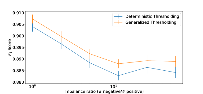
Figure 3: Mean $F_{1}$ scores (over $100$ random training/validation/test splits) of optimal deterministic and stochastic thresholding nearest neighbor classifiers, on the credit card fraud dataset, at various degrees of class imbalance. Error bars denote standard errors, computed over the $100$ random training/validation/test splits.

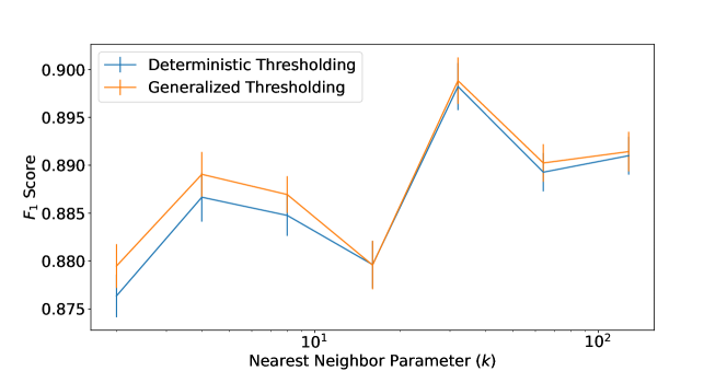
Figure 4: Mean $F_{1}$ scores (over $100$ random training/validation/test splits) of optimal deterministic and stochastic thresholding nearest neighbor classifiers, on the credit card fraud dataset, for various values of the nearest neighbor hyperparameter $k$. Error bars denote standard errors, computed over the $100$ random training/validation/test splits.

The main question we sought to investigate here was whether the theoretical finding, in Theorem 3, that stochastic classification is sometimes necessary in order to obtain optimal prediction performance under general performance metrics, would be visible in real data. To investigate this, we partitioned the dataset randomly into a training subset ($60\%$ of samples), a validation subset ($20\%$ of samples), and a test subset ($20\%$ of samples). We fit a $k$-nearest neighbor regressor (with Euclidean distance as the underlying metric) to the training subset, used the validation subset to select optimal deterministic and generalization thresholds, and then used the test subset to evaluate performance. We evaluated performance in terms of $F_{1}$ score, since it is perhaps the CMM most widely used with imbalanced datasets. We then repeated this experiment with $100$ random train/validation/test splits and report aggregate results over these independent trials.

We generally found that, as predicted by our theoretical results, stochastic thresholding generally outperforms deterministic thresholding by a small but consistent margin. Figure 3 shows that, for fixed nearest neighbor hyperparameter $k=4$, this effect is robust across differing degrees of class imbalance, for imbalance ratios ranging from $1:1$ (perfect balance) to $57:1$ (the full dataset), where class imbalance here was manipulated by down-sampling the negative class. Similarly, Figure 4 shows that this effect is robust over different values of the nearest neighbor hyperparameter $k\in\{2,4,8,16,32,64,128\}$.

References

- Arlot and Bartlett [2011] Sylvain Arlot and Peter L Bartlett. Margin-adaptive model selection in statistical learning. Bernoulli, 17(2):687–713, 2011.
- Audibert and Tsybakov [2007] Jean-Yves Audibert and Alexandre B Tsybakov. Fast learning rates for plug-in classifiers. The Annals of Statistics, 35(2):608–633, 2007.
- Awoyemi et al. [2017] John O Awoyemi, Adebayo O Adetunmbi, and Samuel A Oluwadare. Credit card fraud detection using machine learning techniques: A comparative analysis. In 2017 International Conference on Computing Networking and Informatics (ICCNI), pages 1–9. IEEE, 2017.
- Bennett [1962] George Bennett. Probability inequalities for the sum of independent random variables. Journal of the American Statistical Association, 57(297):33–45, 1962.
- Biau and Devroye [2015] Gérard Biau and Luc Devroye. Lectures on the Nearest Neighbor Method. Springer, 2015.
- Biau et al. [2010] Gérard Biau, Frédéric Cérou, and Arnaud Guyader. Rates of convergence of the functional -nearest neighbor estimate. IEEE Transactions on Information Theory, 56(4):2034–2040, 2010.
- Boucheron et al. [2013] Stéphane Boucheron, Gábor Lugosi, and Pascal Massart. Concentration Inequalities: A Nonasymptotic Theory of Independence. Oxford University Press, 2013.
- Bousquet et al. [2003] Olivier Bousquet, Stéphane Boucheron, and Gábor Lugosi. Introduction to statistical learning theory. In Summer School on Machine Learning, pages 169–207. Springer, 2003.
- Cannings et al. [2019] Timothy I Cannings, Thomas B Berrett, and Richard J Samworth. Local nearest neighbour classification with applications to semi-supervised learning. arXiv preprint arXiv:1704.00642 v3, 2019.
- Cano et al. [2013] Alberto Cano, Amelia Zafra, and Sebastián Ventura. Weighted data gravitation classification for standard and imbalanced data. IEEE Transactions on Cybernetics, 43(6):1672–1687, 2013.
- Chaudhuri and Dasgupta [2014] Kamalika Chaudhuri and Sanjoy Dasgupta. Rates of convergence for nearest neighbor classification. In Advances in Neural Information Processing Systems, pages 3437–3445, 2014.
- Chawla et al. [2002] Nitesh V Chawla, Kevin W Bowyer, Lawrence O Hall, and W Philip Kegelmeyer. SMOTE: synthetic minority over-sampling technique. Journal of Artificial Intelligence Research, 16:321–357, 2002.
- Cortes and Mohri [2004] Corinna Cortes and Mehryar Mohri. AUC optimization vs. error rate minimization. Advances in Neural Information Processing Systems, 16(16):313–320, 2004.
- Cotter et al. [2019a] Andrew Cotter, Heinrich Jiang, and Karthik Sridharan. Two-player games for efficient non-convex constrained optimization. In Algorithmic Learning Theory, pages 300–332. PMLR, 2019a.
- Cotter et al. [2019b] Andrew Cotter, Harikrishna Narasimhan, and Maya R Gupta. On making stochastic classifiers deterministic. Advances in Neural Information Processing Systems (NeurIPS), 2019b.
- Cover and Hart [1967] Thomas Cover and Peter Hart. Nearest neighbor pattern classification. IEEE Transactions on Information Theory, 13(1):21–27, 1967.
- Dembczynski et al. [2013] Krzysztof Dembczynski, Arkadiusz Jachnik, Wojciech Kotlowski, Willem Waegeman, and Eyke Huellermeier. Optimizing the F-measure in multi-label classification: Plug-in rule approach versus structured loss minimization. In Proceedings of the 30th International Conference on Machine Learning. PMLR, 2013.
- Dembczyński et al. [2017] Krzysztof Dembczyński, Wojciech Kotłowski, Oluwasanmi Koyejo, and Nagarajan Natarajan. Consistency analysis for binary classification revisited. In International Conference on Machine Learning, pages 961–969. PMLR, 2017.
- Devroye et al. [1996] Luc Devroye, László Györfi, and Gábor Lugosi. A probabilistic theory of pattern recognition. Springer Science & Business Media, 1996.
- Döring et al. [2018] Maik Döring, László Györfi, and Harro Walk. Rate of convergence of k-nearest-neighbor classification rule. The Journal of Machine Learning Research, 18(227):1–16, 2018.
- Durrett [2010] Rick Durrett. Probability: Theory and Examples. Cambridge university press, fourth edition, 2010.
- Fathony and Kolter [2019] Rizal Fathony and J Zico Kolter. AP-perf: Incorporating generic performance metrics in differentiable learning. arXiv preprint arXiv:1912.00965, 2019.
- Fernández et al. [2018] Alberto Fernández, Salvador García, Mikel Galar, Ronaldo C Prati, Bartosz Krawczyk, and Francisco Herrera. Learning from Imbalanced Data Sets. Springer, 2018.
- Fithian and Hastie [2014] William Fithian and Trevor Hastie. Local case-control sampling: Efficient subsampling in imbalanced data sets. Annals of Statistics, 42(5):1693, 2014.
- Fix and Hodges [1951] Evelyn Fix and Joseph L Hodges. Discriminatory analysis-nonparametric discrimination: consistency properties. Technical report, USAF School of Aviation Medicine, Randolph Field, Texas, 1951.
- Flach [2003] Peter A Flach. The geometry of ROC space: understanding machine learning metrics through roc isometrics. In Proceedings of the 20th International Conference on Machine Learning (ICML-03), pages 194–201, 2003.
- Flach [2016] Peter A Flach. Classifier calibration. In Encyclopedia of Machine Learning and Data Mining. Springer US, 2016.
- Gadat et al. [2016] Sébastien Gadat, Thierry Klein, and Clément Marteau. Classification in general finite dimensional spaces with the k-nearest neighbor rule. The Annals of Statistics, 44(3):982–1009, 2016.
- Gottlieb et al. [2018] L. Gottlieb, A. Kontorovich, and P. Nisnevitch. Near-optimal sample compression for nearest neighbors. IEEE Transactions on Information Theory, 64(6):4120–4128, 2018.
- Gottlieb et al. [2014] Lee-Ad Gottlieb, Aryeh Kontorovich, and Robert Krauthgamer. Efficient classification for metric data. IEEE Transactions on Information Theory, 60(9):5750–5759, 2014.
- Györfi et al. [2002] László Györfi, Michael Kohler, Adam Krzyzak, and Harro Walk. A distribution-free theory of nonparametric regression. Springer Science & Business Media, 2002.
- Hanneke et al. [2020] Steve Hanneke, Aryeh Kontorovich, Sivan Sabato, and Roi Weiss. Universal Bayes consistency in metric spaces. In 2020 Information Theory and Applications Workshop (ITA), pages 1–33. IEEE, 2020.
- He and Ma [2013] Haibo He and Yunqian Ma. Imbalanced Learning: Foundations, Algorithms, and Applications. John Wiley & Sons, 2013.
- Hernández-Orallo et al. [2013] José Hernández-Orallo, Peter Flach, and César Ferri. Roc curves in cost space. Machine learning, 93(1):71–91, 2013.
- James et al. [2013] Gareth James, Daniela Witten, Trevor Hastie, and Robert Tibshirani. An Introduction to Statistical Learning, volume 112. Springer, 2013.
- Joachims [2005] Thorsten Joachims. A support vector method for multivariate performance measures. In Proceedings of the 22nd International Conference on Machine Learning, pages 377–384. ACM, 2005.
- Kontorovich and Weiss [2015] Aryeh Kontorovich and Roi Weiss. A Bayes consistent 1-NN classifier. In Artificial Intelligence and Statistics, pages 480–488. PMLR, 2015.
- Koyejo et al. [2014] Oluwasanmi O Koyejo, Nagarajan Natarajan, Pradeep K Ravikumar, and Inderjit S Dhillon. Consistent Binary Classification with Generalized Performance Metrics. In Advances in Neural Information Processing Systems 27, pages 2744–2752. Curran Associates, Inc., 2014.
- Krawczyk [2016] Bartosz Krawczyk. Learning from imbalanced data: open challenges and future directions. Progress in Artificial Intelligence, 5(4):221–232, 2016.
- Lehmann and Romano [2006] Erich L Lehmann and Joseph P Romano. Testing Statistical Hypotheses. Springer Science & Business Media, 2006.
- Lewis [1995] David D Lewis. Evaluating and optimizing autonomous text classification systems. In SIGIR, volume 95, pages 246–254. Citeseer, 1995.
- Lipton et al. [2014] Zachary C Lipton, Charles Elkan, and Balakrishnan Naryanaswamy. Optimal thresholding of classifiers to maximize f1 measure. In Joint European Conference on Machine Learning and Knowledge Discovery in Databases, pages 225–239. Springer, 2014.
- Liu and Chawla [2011] Wei Liu and Sanjay Chawla. Class confidence weighted knn algorithms for imbalanced data sets. In Pacific-Asia Conference on Knowledge Discovery and Data Mining, pages 345–356. Springer, 2011.
- López et al. [2014] Victoria López, Isaac Triguero, Cristóbal J Carmona, Salvador García, and Francisco Herrera. Addressing imbalanced classification with instance generation techniques: IPADE-ID. Neurocomputing, 126:15–28, 2014.
- Lu et al. [2020] Zhihe Lu, Yongxin Yang, Xiatian Zhu, Cong Liu, Yi-Zhe Song, and Tao Xiang. Stochastic classifiers for unsupervised domain adaptation. In Proceedings of the IEEE/CVF Conference on Computer Vision and Pattern Recognition, pages 9111–9120, 2020.
- Mammen and Tsybakov [1999] Enno Mammen and Alexandre B Tsybakov. Smooth discrimination analysis. The Annals of Statistics, 27(6):1808–1829, 1999.
- Mariani et al. [2018] Giovanni Mariani, Florian Scheidegger, Roxana Istrate, Costas Bekas, and Cristiano Malossi. Bagan: Data augmentation with balancing GAN. arXiv preprint arXiv:1803.09655, 2018.
- McDiarmid [1998] Colin McDiarmid. Concentration. In Probabilistic Methods for Algorithmic Discrete Mathematics, pages 195–248. Springer, 1998.
- Menon et al. [2013] Aditya Menon, Harikrishna Narasimhan, Shivani Agarwal, and Sanjay Chawla. On the statistical consistency of algorithms for binary classification under class imbalance. In International Conference on Machine Learning, pages 603–611, 2013.
- Mitchell [1997] Tom M Mitchell. Machine Learning. McGraw-hill New York, 1997.
- Mohri et al. [2018] Mehryar Mohri, Afshin Rostamizadeh, and Ameet Talwalkar. Foundations of Machine Learning. MIT press, 2018.
- Narasimhan et al. [2014] Harikrishna Narasimhan, Rohit Vaish, and Shivani Agarwal. On the statistical consistency of plug-in classifiers for non-decomposable performance measures. In Advances in Neural Information Processing Systems, pages 1493–1501, 2014.
- Narasimhan et al. [2015] Harikrishna Narasimhan, Harish Ramaswamy, Aadirupa Saha, and Shivani Agarwal. Consistent multiclass algorithms for complex performance measures. In International Conference on Machine Learning, pages 2398–2407. PMLR, 2015.
- Noé et al. [2020] Frank Noé, Gianni De Fabritiis, and Cecilia Clementi. Machine learning for protein folding and dynamics. Current Opinion in Structural Biology, 60:77–84, 2020.
- Pinot et al. [2022] Rafael Pinot, Laurent Meunier, Florian Yger, Cédric Gouy-Pailler, Yann Chevaleyre, and Jamal Atif. On the robustness of randomized classifiers to adversarial examples. Machine Learning, pages 1–33, 2022.
- Rigollet and Tong [2011] Philippe Rigollet and Xin Tong. Neyman-Pearson classification, convexity and stochastic constraints. Journal of Machine Learning Research, 12(Oct):2831–2855, 2011.
- Samworth [2012] Richard J Samworth. Optimal weighted nearest neighbour classifiers. Annals of Statistics, 40(5):2733–2763, 2012.
- Schaefer et al. [2020] Julia Schaefer, Moritz Lehne, Josef Schepers, Fabian Prasser, and Sylvia Thun. The use of machine learning in rare diseases: a scoping review. Orphanet Journal of Rare Diseases, 15(1):1–10, 2020.
- Scott [2012] Clayton Scott. Calibrated asymmetric surrogate losses. Electronic Journal of Statistics, 6:958–992, 2012.
- Stone [1977] Charles J Stone. Consistent nonparametric regression. The Annals of Statistics, pages 595–620, 1977.
- Tong [2013] Xin Tong. A plug-in approach to Neyman-Pearson classification. The Journal of Machine Learning Research, 14(1):3011–3040, 2013.
- Tong et al. [2016] Xin Tong, Yang Feng, and Anqi Zhao. A survey on Neyman-Pearson classification and suggestions for future research. Wiley Interdisciplinary Reviews: Computational Statistics, 8(2):64–81, 2016.
- Tsybakov [2009] Alexandre B Tsybakov. Introduction to Nonparametric Estimation. Revised and extended from the 2004 French original. Translated by Vladimir Zaiats. Springer Series in Statistics. Springer, New York, 2009.
- Van Rijsbergen [1974] Cornelis Joost Van Rijsbergen. Foundation of evaluation. Journal of Documentation, 30(4):365–373, 1974.
- Van Rijsbergen [1979] Cornelis Joost Van Rijsbergen. Information Retrieval. Butterworth-Heinemann, London, 2nd edition, 1979.
- Vapnik and Chervonenkis [2015] Vladimir N Vapnik and A Ya Chervonenkis. On the uniform convergence of relative frequencies of events to their probabilities. In Measures of Complexity, pages 11–30. Springer, 2015.
- Vluymans et al. [2016] Sarah Vluymans, Isaac Triguero, Chris Cornelis, and Yvan Saeys. Eprennid: An evolutionary prototype reduction based ensemble for nearest neighbor classification of imbalanced data. Neurocomputing, 216:596–610, 2016.
- Wang [2020] HaiYing Wang. Logistic regression for massive data with rare events. In International Conference on Machine Learning, pages 9829–9836. PMLR, 2020.
- Wang et al. [2019a] Xiaoyan Wang, Ran Li, Bowei Yan, and Oluwasanmi Koyejo. Consistent classification with generalized metrics. arXiv preprint arXiv:1908.09057, 2019a.
- Wang et al. [2019b] Xin Wang, Hao Helen Zhang, and Yichao Wu. Multiclass probability estimation with support vector machines. Journal of Computational and Graphical Statistics, pages 1–18, 2019b.
- Wu et al. [2022] Jimmy Wu, Yatong Chen, and Yang Liu. Metric-fair classifier derandomization. In International Conference on Machine Learning, pages 23999–24016. PMLR, 2022.
- Yan et al. [2018] Bowei Yan, Sanmi Koyejo, Kai Zhong, and Pradeep Ravikumar. Binary classification with karmic, threshold-quasi-concave metrics. In International Conference on Machine Learning, pages 5531–5540. PMLR, 2018.
- Zhao et al. [2013] Ming-Jie Zhao, Narayanan Edakunni, Adam Pocock, and Gavin Brown. Beyond fano’s inequality: Bounds on the optimal f-score, ber, and cost-sensitive risk and their implications. The Journal of Machine Learning Research, 14(1):1033–1090, 2013.
- Zhu et al. [2015] Yujin Zhu, Zhe Wang, and Daqi Gao. Gravitational fixed radius nearest neighbor for imbalanced problem. Knowledge-Based Systems, 90:224–238, 2015.