Nonequilibrium thermodynamic process with hysteresis and metastable states — A contact Hamiltonian with unstable and stable segments of a Legendre submanifold

Abstract

In this paper, a dynamical process in a statistical thermodynamic system of spins exhibiting a phase transition is described on a contact manifold, where such a dynamical process is a process that a metastable equilibrium state evolves into the most stable symmetry broken equilibrium state. Metastable and the most stable equilibrium states in the symmetry broken phase or ordered phase are assumed to be described as pruned projections of Legendre submanifolds of contact manifolds, where these pruned projections of the submanifolds express hysteresis and pseudo-free energy curves. Singularities associated with phase transitions are naturally arose in this framework as has been suggested by Legendre singularity theory. Then a particular contact Hamiltonian vector field is proposed so that a pruned segment of the projected Legendre submanifold is a stable fixed point set in a region of a contact manifold, and that another pruned segment is a unstable fixed point set. This contact Hamiltonian vector field is identified with a dynamical process departing from a metastable equilibrium state to the most stable equilibrium one. To show the statements above explicitly an Ising type spin model with long-range interactions, called the Husimi-Temperley model, is focused, where this model exhibits a phase transition.

1 Introduction

Contact geometry is known as an odd-dimensional analogue of symplectic geometry [1, 2, 3], and has been studied from viewpoints of pure and applied mathematics [4]. From the pure mathematics side, contact topology[5], contact Riemannian geometry [6], and so on [7] are studied. From the applied mathematics side, geometrization of thermodynamics [8, 9], statistical mechanics [10, 11], applications to information geometry [12, 13, 14], and so on [15, 16, 17, 18, 19] are studied. In particular contact geometric approaches to thermodynamics  [20, 21] and dissipative mechanics [22, 23, 24] are intensively studied. Although the both sides are close in some sense [25], we feel that some gap between them exists, and that profound theorems found in pure mathematics should be applied to such application areas. By filling such a gap, undiscovered notions and facts are expected to be found as in other previous contacts between physics and geometry [26, 27].

Nonequilibrium statistical mechanics and thermodynamics are developing branches of physics, interesting in their own right [28, 29], and their development should prove useful in various research areas, since these branches are closely related to nanotechnology [30], mathematical engineering including Markov chain Monte Carlo methods[31], and so on [32, 33]. Nonequilibrium phenomena are time-dependent thermodynamic phenomena, and some simple cases have successfully been addressed [34, 35]. Although intricate systems are never fully appreciated, some progress in understanding such has been made in proper frameworks. An example is on a dynamical process from a metastable state into a most stable equilibrium state [36]. Another example is to deal with hysteresis curves in magnetic systems [37]. Beyond these, one should expect further progress. As stated above, although considerable activity is being devoted to formulate nonequilibrium statistical thermodynamics, there is little consensus in the literature on its foundation. To establish a foundation of nonequilibrium theory, one might focus on a canonical example as a first step. This is because the Ising model, a canonical model, played a central role in developing equilibrium theory [38]. Choosing a simple toy model appropriately many quantities are evaluated analytically, and insights can be gained from its simplicity. One of such a good model is the Husimi-Temperley model. This is based on the Ising model, by modifying the interaction range from the nearest neighbor one to the global or mean field type. This model, the Husimi-Temperley model, exhibits a phase transition, and several quantities can be calculated analytically [39, 40, 41]. On the one hand, one might be concerned that such long-range interactions are physically irrelevant. On the other hand, one might think that systems with long-range interactions are ubiquitous in the world. Examples of such systems include self-gravitating particles, two-dimensional fluid, and so on [36]. Since these examples exist, the study of a class of statistical systems with long-range interactions is meaningful, where this class includes spin systems with long-range interactions. In this paper this later perspective is adapted.

To formulate nonequilibrium statistical mechanics one might take the attitude that a contact geometric approach is employed  [42, 12, 43]. One of the questions in constructing such a formulation is how to deal with phase transitions [44], and another one is how to introduce dynamics describing nonequilibrium phenomena. In this paper both of these questions are addressed for the case of the Husimi-Temperley model, that is an Ising type model. This model enables many quantities to be expressed analytically, and because of its simplicity physical insights can be gained. One advantage of the use of contact geometry is that Legendre singularity theory [45] is expected to provide a sophisticated tool set to elucidate mechanisms of phase transitions [46, 47].

Outline of this contribution

In this paper analysis of the Husimi-Temperley model is summarized to make this paper self-contained, and then its geometric description is proposed. In this proposal stable and unstable segments of the hysteresis and pseudo-free energy curves are considered. Each curve is identified with a union of pruned segments of a projected Legendre submanifold, where this Legendre submanifold is a $1$-dimensional submanifold of a $3$-dimensional contact manifold. In this framework a thermodynamic phase space is identified with a contact manifold where the contact form restricts vector fields so that the first law of thermodynamics holds, and the time-development of contact Hamiltonian systems is identified with the time-development of thermodynamic processes in thermodynamic phase spaces. The main theorem in this paper and its physical interpretation are informally stated as follows.

Claim 1.1.

(informal version of Theorem 3.1). The integral curves of a contact Hamiltonian vector field on a $3$-dimensional contact manifold connect a unstable segment of a Legendre submanifold and a stable one. Physically this contact Hamiltonian vector field expresses the dynamical process departing from a unstable branch of the hysteresis curve to a stable one. Simultaneously this vector field expresses the dynamical process departing from a unstable branch of the free-energy curve to a stable one.

To explain how to arrive at this claim, a procedure together with calculations of this paper is summarized below. Since this summary is an abstraction of the calculations for the specific model, this summary is seen as a generalization from the specific procedure.

1. Introduce a statistical model (of spins) with a parameter $J_{\,0}\in\mathbb{R}$, let $x\,\in\mathbb{R}$ and $y\,\in\mathbb{R}$ denote a dimensionless applied external field and magnetization, respectively. Then $x$ and $y$ form a pair of thermodynamic conjugate variables. In general, the main task for elucidating thermodynamic properties of a microscopic model is to calculate the corresponding partition function by integrating all the degrees of freedom with some measure. This measure is often chosen as the canonical measure, and the partition function yields the free-energy. Consider the case that a dimensionless free-energy per degree of freedom $\psi_{\,J_{0}}$ is obtained with the so-called saddle point method:

   $$\psi_{\,J_{0}}(x,y^{\,*})\simeq\min_{y}\ \psi_{\,J_{0}}(x,y)=\min_{\mu}\ \psi_{\,J_{0}}(x,y_{\,\mu}^{\,*}),$$

   where $\mu\,\in\mathbb{N}$ is a label for discriminating various local minima of $\psi_{\,J_{0}}$ with respect to $y$, and $y_{\,\mu}^{\,*}$ denotes a local minimum point. In this paper the following form of $\psi_{\,J_{0}}$ is focused:

   $$\psi_{\,J_{0}}(x,y)=J_{\,0}y^{\,2}-\int\check{s}(\Delta)\,\mathrm{d}\,\Delta,\qquad\Delta:=2J_{\,0}y+x,$$

   where $\check{s}$ is a function, and $\check{s}(\Delta)=\tanh(\Delta)$ for the Husimi-Temperley model.

2. Introduce the $3$-dimensional contact manifold $(T^{\,*}\mathbb{R}\times\mathbb{R},\lambda)$ whose coordinates are $(x,y,z)$ so that $\lambda=\mathrm{d}z+y\,\mathrm{d}x$ is a contact $1$-form. Then a union of (metastable) equilibrium states are identified with a Legendre submanifold. The coordinate expression of a (metastable) equilibrium state is $(x,y_{\mu}^{\,*}(x),z(x,y_{\,\mu}^{\,*}(x)))$ labeled by $\mu$, where

   $$\frac{\partial\psi_{\,J_{0}}}{\partial y_{\,\mu}^{\,*}}=2\left(y_{\,\mu}^{\,*}-\check{s}(\Delta_{\,\mu}^{\,*})\,\right)J_{\,0}=0,\quad\frac{\partial\psi_{\,J_{0}}}{\partial x}=-y_{\,\mu}^{\,*},\quad z=\psi_{\,J_{0}}(x,y_{\,\mu}^{\,*}),\qquad\Delta_{\,\mu}^{\,*}:=2J_{\,0}y_{\,\mu}^{\,*}+x,$$

   with $\check{s}$ constituting a self-consistent equation $y_{\,\mu}^{\,*}=\check{s}(\Delta_{\,\mu}^{\,*})$. Self-consistent equations are often derived in the study of systems with phase transitions, where a phase transition is equivalent to a bifurcation of the solution of the self-consistent equation. From this construction, the hysteresis curve is nothing but the projection of the Legendre submanifold onto the $(x,y)$-plane up to sign convention. In addition, the pseudo-free energy curve is the projection of the Legendre submanifold onto the $(x,z)$-plane. The set of multiple branches of the hysteresis curve is recognized as a multi-valued function of $x$, $x\mapsto y_{\,\mu}^{\,*}=y_{\,\mu}^{\,*}(x)$. If this multi-valued function is invertible, then $x=x(y_{\,\mu}^{\,*})$ exists, where the function $y_{\,\mu}^{\,*}\mapsto x(y_{\,\mu}^{\,*})$ may be a single-valued function. In the Husimi-Temperley model $x$ can explicitly be written in terms of $y_{\mu}^{\,*}$ on the Legendre submanifold, and the multiple branches of the hysteresis curve can be drawn by varying the value of $y_{\,\mu}^{\,*}$ continuously in the recognition that the graph $(x,y_{\,\mu}^{\,*}(x))$ is depicted by $(x(y_{\,\mu}^{\,*}),y_{\,\mu}^{\,*})$, where $x:y_{\,\mu}^{\,*}\mapsto x(y_{\,\mu}^{\,*})$ is a single-valued function. Thus the Legendre submanifold whose projections are labeled by $\mu$ can be treated as a one submanifold, rather than multiple submanifolds. The projection of the Legendre submanifold onto the $(x,z)$-plane expresses a pseudo-free energy as a multi-valued function. This multi-valued function expresses a set of metastable, unstable, and most stable equilibrium states. These projections in the symmetry broken phase are depicted in Fig. 1. Note that $\psi_{\,J_{0}}$ is not convex with respect to $x$  (see Remark 2.1 and Ref. [48]), whereas $\psi_{\,J_{0}}$ is convex with respect to $y$ in the high temperature phase  (see Remark 2.1 together with Fig. 7).

   Figure 1: Unpruned projections of the Legendre submanifold in the low temperature phase (symmetry broken phase). (Left) The $(x,z)$-plane. (Right) The $(x,y)$-plane.

3. Prune the top branch on the $(x,z)$-plane of the projection (see Fig. 2). This pruning procedure is equivalent to prune the middle segment passing through $(0,0)$ on the $(x,y)$-plane. Then the resultant disconnected segments of the projection of the Legendre submanifold yield disconnected hysteresis and pseudo-free energy curves that are expected to be observed in experiments.

   Figure 2: Pruned segments of the projections of the Legendre submanifold in the low temperature phase (symmetry broken phase). The regions ${\cal I}^{\,\mp}$ are such that ${\cal I}^{\,-}:=\{\,x\in\mathbb{R}_{\,<0}\,|\,\psi_{\,1}(x)<\psi_{\,2}(x)\,\}\subset\mathbb{R}$ and ${\cal I}^{\,+}:=\{\,x\in\mathbb{R}_{\,>0}\,|\,\psi_{\,1}(x)<\psi_{\,2}(x)\,\}\subset\mathbb{R}$, where $\psi_{\,\mu}(x)=\psi_{\,J_{0}}(x,y_{\,\mu}^{\,*}(x))$ is an abbreviation. (Left) The $(x,z)$-plane. (Right) The $(x,y)$-plane.

4. Choose a contact Hamiltonian

   $$h(x,y,z)=-\,\psi_{\,0}(x)(z-\psi_{\,1}(x))(z-\psi_{\,2}(x))^{\,2},$$

   where $\psi_{\,0}$ is a positive function of $x$. Its corresponding contact Hamiltonian vector field expresses the dynamical process on the $(x,y)$- and $(x,z)$-planes. The pruned projections of the Legendre submanifold are shown to be stable and unstable (see Fig. 3). This gives Claim 1.1.

   Figure 3: Contact Hamiltonian vector field that expresses the dynamical process in the low temperature phase (symmetry broken phase). The fixed point sets are pruned segments of the projections of the Legendre submanifold. (Left) The $(x,z)$-plane. (Right) The $(x,y)$-plane.

In the case where there is only one single-valued function of $x$ one can find a contact Hamiltonian such that the corresponding segment of the projection of the Legendre submanifold is attractor as has been argued in Refs. [12, 25].

As a corollary of Claim 1.1, the following is obtained.

Claim 1.2.

(informal version of Corollary 3.1). When pruning the unstable segments of the projected Legendre submanifold, as the set of attractors of the contact Hamiltonian systems, the cusp of the shape $\wedge$ appears on the $(x,z)$-plane, and the kink of the shape $\lrcorner\ulcorner$ appears on the $(x,y)$-plane (see Fig. 4).

Figure 4: Union of the stable pruned projections of the Legendre submanifold in the low temperature phase (symmetry broken phase). (Left) The $(x,z)$-plane. The cusp of the shape $\wedge$ appears, and the existence of this cusp corresponds to the existence of the $1$st-order phase transition. (Right) The $(x,y)$-plane. The kink of the shape $\lrcorner\ulcorner$ appears, and this expresses the experimental observation where the hysteresis curve is ruined by perturbation.

From Claim 1.2, the long-time evolution of the proposing contact Hamiltonian system plays a similar role of the Maxwell construction discussed in thermodynamics and the role of the convexification by the Legendre transforms.

The rest of this paper is organized as follows. In Section 2, some preliminaries are provided in order to keep this paper self-contained. They are basics of contact geometry including projections of Legendre submanifolds, contact Hamiltonian systems, and so on. In addition the so-called Husimi-Temperley model and its thermodynamics are briefly summarized. In Section 3, after arguing that metastable and unstable equilibrium states are described as a Legendre submanifold in a contact manifold, pruned segments of the projected Legendre submanifold are introduced. Then, a contact Hamiltonian vector field is introduced where this vector field expresses the dynamical process under the case that the unstable and stable segments of the hysteresis curve exist in the symmetry broken phase. Section 4 summarizes this paper and discusses some future works. In Appendix A, some other contact Hamiltonian systems are discussed.

2 Preliminaries

This section is intended to provide a brief summary of the necessary background, and consists of $2$ parts. They are about contact geometry, and about thermodynamic properties of the Husimi-Temperley model.

2.1 Contact and symplectic geometries

To argue contact geometry of nonequilibrium thermodynamics, some known facts on contact and symplectic geometries are summarized and notations are fixed here [1, 2]. Various formulas and tools developed in differential geometry are known [26, 27]. For example, the Lie derivative of a $k$-form $\alpha$ along a vector field $X$ can be written as ${\cal L}_{X}\alpha=\mathrm{d}\imath_{\,X}\alpha+\imath_{\,X}\mathrm{d}\alpha$, where $\mathrm{d}$ is the exterior derivative and $\imath_{\,X}$ the interior product with $X$. This is known as the Cartan formula.

Let ${\cal C}$ be a $(2n+1)$-dimensional manifold ($n=1,2,\ldots$), and $\lambda$ a $1$-form on ${\cal C}$ such that

$$\lambda\wedge\underbrace{\mathrm{d}\lambda\wedge\cdots\wedge\mathrm{d}\lambda}_{n}\neq 0,\quad\mbox{at any point on ${\cal C}$}.$$

Then this $\lambda$ is referred to as a contact form. Notice that another $1$-form $f\,\lambda$ with $f$ being a non-vanishing function is also a contact form if $\lambda$ is contact. If a $2n$-dimensional vector space $E\subset T_{\,p}{\cal C}$ is written by $E=\ker\lambda$ with $\ker\lambda=\{\ X\in T_{p}{\cal C}\ |\ \lambda(X)=0\ \}$ around $p\in{\cal C}$, then the pair $({\cal C},\ker\lambda)$ is referred to as a $(2n+1)$-dimensional contact manifold (in the wider sense), where $\lambda(X)$ denotes the pairing between $\lambda$ and $X$. According to the Darboux theorem, there exist coordinates $(x,y,z)$ such that

$$\lambda=\mathrm{d}z-\sum_{a=1}^{n}y_{\,a}\,\mathrm{d}x^{\,a},\quad\mbox{or}\quad\lambda=\mathrm{d}z+\sum_{a=1}^{n}y_{\,a}\,\mathrm{d}x^{\,a},$$ (1)

where $x=(x^{\,1},\ldots,x^{\,n})$ and $y=(y_{\,1},\ldots,y_{\,n})$. These coordinates are referred to as canonical or Darboux coordinates. If there exists such a contact form globally over ${\cal C}$, then the pair $({\cal C},\lambda)$ is referred to as a contact manifold (in the narrower sense). In Section 3 of this paper, this case, $\lambda$ is globally defined, is considered and contact manifolds are written as $({\cal C},\lambda)$. One typical contact manifold is given as $T^{\,*}\mathbb{R}^{n}\times\mathbb{R}$ with some $1$-form.

On a contact manifold $({\cal C},\lambda)$, there exists a vector field $R$ that satisfies

$$\imath_{\,R}\,\mathrm{d}\lambda=0,\qquad\mbox{and}\qquad\imath_{\,R}\lambda=1.$$

This $R$ is referred to as the Reeb vector field, and is uniquely determined for a fixed $\lambda$. This is written as $R=\partial/\partial z$ in the canonical coordinates such that $\lambda$ is written as (1).

A contact vector field $X$ is a vector field on a contact manifold $({\cal C},\lambda)$ that preserves the contact structure $\ker\lambda$, ${\cal L}_{\,X}\lambda=f\lambda$ with $f$ being a non-vanishing function. There is a way to specify a contact vector field with a function described below. The contact Hamiltonian vector field $X_{\,h}$ associated with a function $h$ is the uniquely determined vector field such that

$$\imath_{X_{\,h}}\lambda=h,\qquad\lambda\wedge{\cal L}_{X_{\,h}}\lambda=0,$$ (2)

where the second equation reduces to

$$\imath_{\,X_{h}}\mathrm{d}\lambda=-\,(\mathrm{d}h-(Rh)\lambda),$$

which is shown by applying $\imath_{\,R}$ and the Cartan formula. The function $h$ is referred to as a contact Hamiltonian. Note that there are some sign conventions on defining contact Hamiltonian vector fields. The coordinate expression of $X_{\,h}$ is obtained as follows. Let $(x,y,z)$ be canonical coordinates such that $\lambda=\mathrm{d}z-\sum_{a=1}^{n}y_{\,a}\mathrm{d}x^{\,a}$ in (1). Then from (2), one has

$$X_{\,h}=\sum_{a=1}^{n}\left(\dot{x}^{\,a}\frac{\partial}{\partial x^{\,a}}+\dot{y}_{\,a}\frac{\partial}{\partial y_{\,a}}\right)+\dot{z}\frac{\partial}{\partial z},$$

where $\dot{x}$, $\dot{y}$, and $\dot{z}$ are the functions

$$\dot{x}^{\,a}=-\,\frac{\partial h}{\partial y_{\,a}},\quad\dot{y}_{\,a}=\frac{\partial h}{\partial x^{\,a}}+y_{\,a}\frac{\partial h}{\partial z},\quad\dot{z}=h-\sum_{b=1}^{n}y_{\,b}\frac{\partial h}{\partial y_{\,b}},\qquad a=1,\ldots,n.$$

Identifying $\dot{\ }=\mathrm{d}/\mathrm{d}t$ and $t\in{\cal I}$, $({\cal I}\subseteq\mathbb{R})$, one has that $X_{\,h}$ expresses a dynamical system. This $t$ will be identified with time in Section 3. This dynamical system is referred to as a contact Hamiltonian system associated with $h$. For $3$-dimensional contact manifolds, one can drop the subscripts and superscripts as

$$\dot{x}=-\,\frac{\partial h}{\partial y},\quad\dot{y}=\frac{\partial h}{\partial x}+y\,\frac{\partial h}{\partial z},\quad\dot{z}=h-y\,\frac{\partial h}{\partial y}.$$

In the case of $\lambda=\mathrm{d}z+y\,\mathrm{d}x$ for $3$-dimensional manifolds, one derives

$$\dot{x}=\frac{\partial h}{\partial y},\quad\dot{y}=-\,\frac{\partial h}{\partial x}+y\,\frac{\partial h}{\partial z},\quad\dot{z}=h-y\,\frac{\partial h}{\partial y}.$$ (3)

On contact manifolds, some special submanifolds play important roles. Given a $(2n+1)$-dimensional contact manifold $({\cal C},\lambda)$, an $n$-dimensional submanifold such that $\phi^{\,*}\lambda=0$ is referred to as a Legendre submanifold ( Legendrian submanifold ), where $\phi^{\,*}$ is the pullback of an embedding $\phi$. Such a submanifold is generated by a function, and an example is shown in Example 2.1. If the dimension of a Legendre submanifold is unity, then this submanifold is referred to as a Legendre curve.

Example 2.1.

Let $(\mathbb{R}^{\,3},\lambda)$ be a $3$-dimensional contact manifold, $(x,y,z)$ its coordinates, and $\lambda=\mathrm{d}z\mp y\,\mathrm{d}x$. In addition, let $\psi_{\,\mathrm{R}}$ be a function of $x$. Then

$$\phi\,{\cal A}_{\,\psi_{\mathrm{R}}}=\left\{\ (x,y,z)\in\mathbb{R}^{\,3}\ \bigg{|}\ z=\psi_{\,\mathrm{R}}(x),\quad\mbox{and}\quad y=\pm\frac{\mathrm{d}\psi_{\,\mathrm{R}}}{\mathrm{d}x}\ \right\}$$

is a Legendre submanifold generated by $\psi_{\,\mathrm{R}}$ due to $\phi^{\,*}\lambda=0$ and $\dim(\phi\,{\cal A}_{\psi_{\mathrm{R}}})=1$.

Another example being relevant to this paper is as follows.

Example 2.2.

Let $(\mathbb{R}^{\,3},\lambda)$ be a $3$-dimensional contact manifold, $(x,y,z)$ its coordinates, and $\lambda=\mathrm{d}z-y\,\mathrm{d}x$. In addition, let $\psi_{\,\mathrm{I}}$, $f_{\,\mathrm{I}}$, and $\Delta$ be the functions

$$\psi_{\,\mathrm{I}}(x,y)=y^{\,2}-f_{\,\mathrm{I}}(\Delta),\quad\Delta(x,y)=2y-x.$$

Then the embedded manifold

$$\phi\,{\cal A}_{\,\psi_{\,\mathrm{I}}}=\left\{\ (x,y,z)\in\mathbb{R}^{\,3}\ \bigg{|}\ z=\psi_{\,\mathrm{I}}(x,y),\quad\mbox{and}\quad y=\frac{\mathrm{d}f_{\,\mathrm{I}}}{\mathrm{d}\Delta}(\Delta(x,y)),\quad\mbox{where}\ x\in{\cal I}\ \right\},$$ (4)

is a Legendre submanifold, where $y=\mathrm{d}f_{\,\mathrm{I}}/\mathrm{d}\Delta$ can be treated as an algebraic equation for $y$ with $x$ being a continuous parameter, and ${\cal I}\subset\mathbb{R}$ is a region in which the real solution for $y$ exists. The submanifold (4) is verified to be Legendrian as $\dim(\phi\,{\cal A}_{\,\psi_{\,\mathrm{I}}})=1$ and

$$\phi^{\,*}\lambda = \mathrm{d}\,(\phi^{\,*}z)-(\phi^{\,*}y)\,\mathrm{d}(\phi^{\,*}x)$$

$$= \frac{\partial\psi_{\,\mathrm{I}}}{\partial x}\mathrm{d}x+\frac{\partial\psi_{\,\mathrm{I}}}{\partial y}\mathrm{d}y-\frac{\mathrm{d}f_{\,\mathrm{I}}}{\mathrm{d}\Delta}\mathrm{d}x$$

$$= -\frac{\mathrm{d}f_{\,\mathrm{I}}}{\mathrm{d}\Delta}\frac{\partial\Delta}{\partial x}\mathrm{d}x+\left(2y-\frac{\mathrm{d}f_{\,\mathrm{I}}}{\mathrm{d}\Delta}\frac{\partial\Delta}{\partial y}\right)\mathrm{d}y-\frac{\mathrm{d}f_{\,\mathrm{I}}}{\mathrm{d}\Delta}\mathrm{d}x$$

$$= 0.$$

Similarly, for the case that

$$\lambda=\mathrm{d}z+y\,\mathrm{d}x,\quad\psi_{\,\mathrm{I}}=y^{\,2}-f_{\,\mathrm{I}}(\Delta),\quad\Delta=-2\,y-x,$$

the embedded submanifold

$$\phi\,{\cal A}_{\,\psi_{\,\mathrm{I}}}=\left\{\ (x,y,z)\in\mathbb{R}^{\,3}\ \bigg{|}\ z=\psi_{\,\mathrm{I}}(x,y),\quad\mbox{and}\quad y=-\frac{\mathrm{d}f_{\,\mathrm{I}}}{\mathrm{d}\Delta}(\Delta(x,y)),\quad\mbox{where}\ x\in{\cal I}\ \right\},$$

is Legendrian. In some physical context, the algebraic equation above is derived as a self-consistent equation for determining the value of an order parameter in statistical mechanics (see around (15)).

In Example 2.2 with $\lambda=\mathrm{d}z-y\,\mathrm{d}x$, it follows that

$$\frac{\partial\psi_{\,\mathrm{I}}}{\partial y}=2y-2\frac{\mathrm{d}f_{\,\mathrm{I}}}{\mathrm{d}\Delta}=0\qquad\mbox{on $\phi{\cal A}_{\,\psi_{\mathrm{I}}}$ },$$

implying that $y$ on the Legendre submanifold is written by the solution to $\partial\psi_{\,\mathrm{I}}/\partial y=0$, and that the solution is written in terms of the derivative $y=\mathrm{d}f_{\,\mathrm{I}}/\mathrm{d}\Delta$. This structure motivates the following generalization from Example 2.2.

Example 2.3.

Let $(T^{\,*}\mathbb{R}\times\mathbb{R},\lambda)$ be a $3$-dimensional contact manifold with $\lambda=\mathrm{d}z+y\,\mathrm{d}x$ where $(x,y,z)$ its coordinates. In addition, let $\psi_{\,\mathrm{II}}$ be a function of $(x,y)$. Then the embedded manifold expressed in coordinates

$$\phi\,{\cal A}_{\,\psi_{\,\mathrm{II}}}=\left\{\ (x,y,z)\ \bigg{|}\ z=\psi_{\,\mathrm{II}}(x,y),\ y=-\frac{\partial\psi_{\,\mathrm{II}}}{\partial x},\ \frac{\partial\psi_{\,\mathrm{II}}}{\partial y}=0.\quad\mbox{where}\ x\in{\cal I}\ \right\},$$ (5)

is a Legendre submanifold, where $\partial\psi_{\,\mathrm{II}}/\partial y=0$ can be treated as an algebraic equation for $y$ with $x$ being a parameter, and ${\cal I}\subset\mathbb{R}$ is a region in which the real solution for $y$ exists. This submanifold is Legendrian due to $\dim(\phi\,{\cal A}_{\,\psi_{\,\mathrm{II}}})=1$ and $\phi^{\,*}\lambda=0$.

In what follows some projections of Legendre submanifolds are defined. Consider first the cotangent bundle $T^{\,*}\mathbb{R}$. Let $x$ be a coordinate of $\mathbb{R}$, and $y$ a coordinate of $T_{\,x}^{\,*}\mathbb{R}$. The so-called Liouville $1$-form is expressed as $\alpha=y\,\mathrm{d}x$, inducing a symplectic form expressed as $\omega=\mathrm{d}\alpha=\mathrm{d}y\wedge\mathrm{d}x$. Second, let $z$ be a coordinate of another $\mathbb{R}$. Then take the $3$-dimensional contact manifold, $(T^{\,*}\mathbb{R}\times\mathbb{R},\lambda)$ where $\lambda=\mathrm{d}z\mp\alpha$. On this contact manifold a Legendre submanifold, or Legendre curve, is identified with an embedded $1$-dimensional curve in the $3$-dimensional manifold, and its projection onto a plane could yield some singularities. The projection of the Legendre curve onto the $(x,y)$-plane is referred to as a Lagrange map, and that onto the $(x,z)$-plane as a Legendre map. The image of a Legendre map is referred to as the wave front of the Legendre curve.

Example 2.4.

For the case of $\lambda=\mathrm{d}z\mp y\,\mathrm{d}x$ on $T^{\,*}\mathbb{R}\times\mathbb{R}$, the wave front of the Legendre curve generated by $\psi_{\,\mathrm{R}}$ being a (single-valued) function depending on $x$

$$\phi{\cal A}_{\,\psi_{\mathrm{R}}}=\left\{\ (x,y,z)\ \bigg{|}\ y=\pm\frac{\mathrm{d}\psi_{\,\mathrm{R}}}{\mathrm{d}x}(x),\quad\mbox{and}\quad z=\psi_{\,\mathrm{R}}(x)\ \right\}$$

is the graph $(x,\psi_{\,\mathrm{R}}(x))$ on the $(x,z)$-plane. Here there is no singularity associated with this projection provided that $\psi_{\,\mathrm{R}}$ is smooth.

Example 2.5.

For the case of $\lambda=\mathrm{d}z-y\,\mathrm{d}x$, the wave front of the Legendre curve expressed in coordinates

$$\phi{\cal A}_{\,\psi_{\,\mathrm{I}}^{\,\prime}}=\left\{\ (x,y,z)\ \bigg{|}\ z=y^{2}-\frac{\Delta^{\,3}}{3},\ y=\Delta^{\,2},\quad\mbox{where}\ \Delta(x,y)=2y-x,\ \mbox{and}\ \frac{-1}{8}\leq x\ \right\}$$ (6)

is obtained as follows (see Example 2.2, and take $f(\Delta)=\Delta^{\,3}/3$ with $\lambda=\mathrm{d}z-y\,\mathrm{d}x$). First the conditions $y=\Delta^{\,2}=(2y-x)^{\,2}$, and $-1/8\leq x$ yield on the $(x,y)$-plane as the image of the Lagrange curve

$$y_{\,\pm}(x)=\frac{4x+1\pm\sqrt{1+8x}}{8},\quad\mbox{for}\quad-\frac{1}{8}\leq x,$$

which can be seen as a multi-valued function of $x$. Each branch of this multi-valued function is jointed at $x=-1/8$, as can be verified from $y_{\,+}(-1/8)=y_{\,-}(-1/8)=1/16$. Second, $z=y^{\,2}-\Delta^{\,3}/3$ is drawn on the $(x,z)$-plane as

$$z(x,y_{\,\pm}(x))=y_{\,\pm}(x)^{\,2}-\frac{y_{\,\pm}(x)^{\,3/2}}{3}.$$

Hence, the wave front is $(x,z_{\,+}(x))\cup(x,z_{\,-}(x))$, where $z_{\,\pm}(x)=z(x,y_{\,\pm}(x))$.

In Fig.5, the projections of the Legendre curve onto various planes are shown. A singular point appears at $x=-1/8$ on the wave front. The projection onto the $(x,z)$-plane can be seen as a double-valued function. This view will be used in analyzing a dynamical process in Section 3.

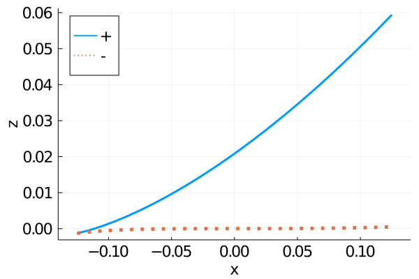
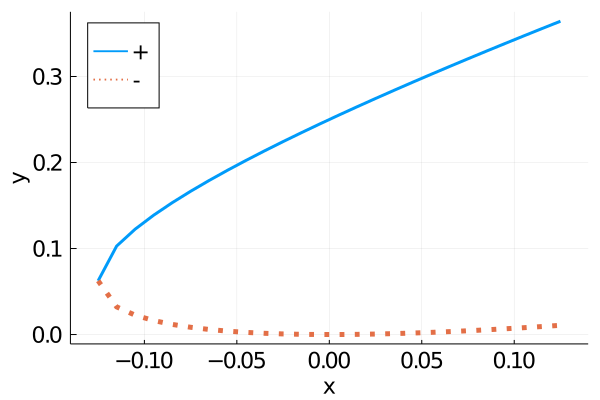
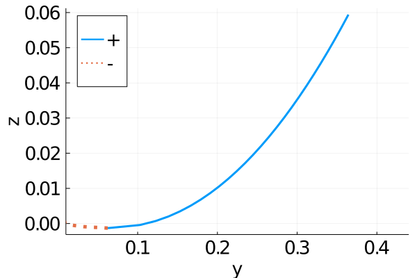
Figure 5: Projection of (6), where $+$ and $-$ denote the lines obtained by $y_{\,+}(x)$ and $y_{\,-}(x)$, respectively. (Left) Projection onto the $(x,z)$-plane, the wave front. (Middle) Projection onto the $(x,y)$-plane, the image of the Lagrange map. (Right) Projection onto the $(y,z)$-plane.

2.2 Thermodynamics of the Husimi-Temperley model

In this subsection an Ising type spin system is introduced, and then its thermodynamic properties derived with canonical statistical mechanics are summarized. The aim of this subsection is to introduce a toy model, where that model should be appropriate in the sense that most of quantities are analytically obtained and introduced quantities are physically interpretable. In Section 3, geometric analysis of this model will be shown.

Consider a lattice whose total number of lattice points is $N$. At the lattice point specified by $i\in\{1,\ldots,N\}\subset\mathbb{N}$ put a spin variable $\sigma_{\,i}=\pm 1$, and then $\sigma:=(\sigma_{\,1},\ldots,\sigma_{\,N})$. The space of the spin variables is denoted ${\cal S}=\{\pm 1\}^{\,N}$, so that $\sigma\in{\cal S}$. The total energy defined for this system is introduced as

$${\cal H}(\sigma)=-\frac{J_{\,0}}{N}\sum_{i=1}^{N}\sum_{j=1}^{N}\sigma_{\,i}\sigma_{\,j}-H\sum_{i=1}^{N}\sigma_{\,i},$$ (7)

where $J_{\,0}\in\mathbb{R}$ is constant expressing the strength of spin interactions, and $H\in\mathbb{R}$ constant expressing an externally applied magnetic field. This ${\cal H}(\sigma)$ has the physical dimension of energy by fixing the physical dimensions of $J_{\,0}$ and $H$. Equation (7) is seen as a function, ${\cal H}:{\cal S}\to\mathbb{R}$. This model is referred to as the Husimi-Temperley model. To elucidate thermodynamic properties of the model, introduce $m:{\cal S}\to\mathbb{R}$ such that

$$m(\sigma)=\frac{1}{N}\sum_{i=1}^{N}\sigma_{\,i},$$

which is an order parameter. The variables $m$ and $H$ form a thermodynamic conjugate pair.

The canonical statistical mechanics is then applied to the Husimi-Temperley model so that thermodynamic properties of this model are elucidated, where the heat bath temperature is denoted by $T>0$. The main task is to calculate the partition function

$$Z=\sum_{\sigma_{1}=\pm 1}\cdots\sum_{\sigma_{N}=\pm 1}\mathrm{e}^{\ -\,\beta{\cal H}(\sigma)}=\sum_{\sigma_{1}=\pm 1}\cdots\sum_{\sigma_{N}=\pm 1}\ \mathrm{e}^{\ \beta J_{\,0}\left(\sum_{l=1}^{N}\sigma_{l}\right)^{\,2}/\,N}\,\mathrm{e}^{\,\beta H\sum_{l=1}^{N}\sigma_{\,l}},$$

where $\beta$ has been defined by $\beta=1/(k_{\mathrm{B}}T)$ with $k_{\,\mathrm{B}}$ being the Boltzmann constant. In the following the so-called saddle point method for Gaussian integral is applied so that an approximate expression of $Z$ is obtained for $N\gg 1$. Under this approximation the free energy obtained from that $Z$ yields various thermodynamic quantities by differentiation.

The expression of $Z$ reduces as follows. The identity

$$\mathrm{e}^{\ bs^{\,2}}=\int_{\mathbb{R}}\frac{\mathrm{d}\varpi}{\sqrt{2\pi}}\mathrm{e}^{\ -\varpi^{\ 2}+2\varpi\sqrt{b}\,s},\quad s\in\mathbb{R}$$

with substitutions $b=\beta J_{\,0}/N$ and $s=\sum_{a=1}^{N}\sigma_{a}$ yields

$$Z=\int_{\mathbb{R}}\frac{\mathrm{d}\varpi}{\sqrt{2\pi}}\mathrm{e}^{\ -\varpi^{\ 2}}\left[2\cosh\left(2\varpi\sqrt{\frac{\beta J_{\,0}}{N}}+\beta H\right)\right]^{\,N}.$$

Furthermore, the change of variables from $\varpi$ to $\xi$ so that $\varpi=\sqrt{N}\xi$, one has

$$Z=\sqrt{\frac{N}{2\pi}}\int_{\mathbb{R}}\,\mathrm{d}\xi\exp\left[\,-\,N\left[\,\xi^{\,2}-\ln\left(2\,\cosh\left(2\xi\sqrt{\beta J_{\,0}}+\beta H\,\right)\,\right)\,\right]\right].$$

In the limit $N\gg 1$, the expression of $Z$ above reduces to

$$Z\simeq\exp\left[\,-\,N\min_{\xi\in\mathbb{R}}\left[\,\xi^{\,2}-\ln\left(2\,\cosh\left(2\xi\sqrt{\beta J_{\,0}}+\beta H\,\right)\,\right)\,\right]\right],$$

where some irrelevant constants have been omitted. This approximation is known as the saddle point method. Under this approximation the free energy ${\cal F}=-k_{\,\mathrm{B}}T\ln Z$ is

$${\cal F}\simeq{\cal F}^{\,\mathrm{saddle}},\quad{\cal F}^{\,\mathrm{saddle}}(T,H;\beta,J_{\,0})=k_{\,\mathrm{B}}TN\min_{\xi\in\mathbb{R}}\left[\,\xi^{\,2}-\ln\left(2\,\cosh\left(2\xi\sqrt{\beta J_{\,0}}+\beta H\,\right)\,\right)\,\right].$$

This expression is rewritten by introducing the variable $y$ satisfying $\xi=y\sqrt{\beta J_{\,0}}$ as

$${\cal F}^{\,\mathrm{saddle}}(T,H;\beta,J_{\,0}) = k_{\,\mathrm{B}}TN\min_{y\in\mathbb{R}}\left[\,\beta J_{\,0}y^{\,2}-\ln\left(2\,\cosh\left(2\beta J_{\,0}y+\beta H\,\right)\,\right)\,\right]$$ (8)

$$= Nf_{\,\beta,J_{\,0}}(x,y^{\,*}),$$ (9)

where

$$x = H,$$ (10)

$$y^{\,*} = \arg\min_{y\in\mathbb{R}}f_{\,\beta,J_{\,0}}(x,y),$$ (11)

$$f_{\,\beta,J_{\,0}}(x,y) = J_{\,0}y^{\,2}-\frac{1}{\beta}\ln\left(2\,\cosh\left(2\beta J_{\,0}\,y+\beta x\,\right)\,\right),$$ (12)

From (9), the physical meaning of $f_{\,\beta,J_{\,0}}(x,y^{\,*})$ is the value of the free energy per degree of freedom. From (9) and (12), $f_{\,\beta,J_{\,0}}(x,y)$ can be interpreted as a relaxation or extension of $f_{\,\beta,J_{\,0}}(x,y^{\,*})$, where $y^{\,*}$ is relaxed to $y\in\mathbb{R}$. This function $f_{\,\beta,J_{\,0}}:\mathbb{R}^{\,2}\to\mathbb{R}$ is referred to as a pseudo-free energy (per degree of freedom) in this paper. The dissimilarity between pseudo-free energy and free energy is that the convexity of pseudo-free energy is not guaranteed.

The $y^{\,*}$ obtained as (11) is chosen from $\{y_{\,\mu}^{\,*}\,|\,\mu=1,2,3\}$, where $y_{\,\mu}^{\,*}$ satisfies

$$\left.\frac{\partial f_{\,\beta,J_{\,0}}}{\partial y}\right|_{y_{\,\mu}^{\,*}}=0,$$ (13)

with $\mu\in\mathbb{N}$ denoting a label for a solution to (13). The reason for introducing labels $\mu$ is to take into account the possibility that the algebraic equation (13) has at most countably many solutions. This equation, (13), is explicitly expressed as

$$y_{\,\mu}^{\,*}-\tanh(2\beta J_{\,0}y_{\,\mu}^{\,*}+\beta x\,)=0,\qquad\mu=1,2,\ldots.$$ (14)

Notice that $y^{\,*}$ satisfies (14), since $y^{\,*}$ is chosen from possible $y_{\,\mu}^{\,*}$, $(\mu=1,2,\ldots)$. One way to solve (14) is to find intersection points of the curve and the line on the $(y,s)$-plane,

$$s_{\,x;\beta,J_{\,0}}(y)=\tanh(2\beta J_{\,0}y+\beta x\,),\qquad\mbox{and}\qquad s(y)=y.$$ (15)

In Fig. 6, the intersection points discussed above are shown.

Figure 6: Intersection points of (15) are the solutions to (14). (Left) There are $3$ intersection points in the low temperature phase ($\beta=1.0$, $J_{\,0}=1.0$, $x=0.1$), which are denoted by $y_{\,1}^{\,*},y_{\,2}^{\,*},y_{\,3}^{\,*}$. (Right) There is $1$ intersection point in the high temperature phase ($\beta=0.4$, $J_{\,0}=1.0$, $x=0.1$), which is denoted by $y_{\,1}^{\,*}$.

Although an explicit expression for $y_{\,\mu}^{\,*}$ as a function of $x,\beta,J_{\,0}$ is not obtained, a condition when the number of solutions changes is found, that is obtained from

$$\left.\frac{\mathrm{d}s_{\,x;\beta,J_{\,0}}}{\mathrm{d}y}\right|_{\,y=\widetilde{y}^{\,*}}\quad\left\{\begin{array}[]{cl}>1&\mbox{the number of solutions is $3$,}\\ =1&\mbox{the critical point,}\\ <1&\mbox{the number of solutions is $1$ }\end{array}\right.,$$ (16)

where $\widetilde{y}^{\,*}$ is the solution of (14) near $y=0$. Hence the critical point is determined by the tangency condition $\mathrm{d}s_{\,x;\beta,J_{\,0}}/\mathrm{d}y=1$ at $y=\widetilde{y}^{\,*}$, and is expressed as

$$\left.\frac{\mathrm{d}s_{\,x;\beta,J_{\,0}}}{\mathrm{d}y}\right|_{\,y=\widetilde{y}^{\,*}}=\left.\frac{2\beta J_{\,0}}{\cosh^{\,2}(2\beta J_{\,0}y+\beta x)}\right|_{\,y=\widetilde{y}^{\,*}}=1.$$ (17)

For example, consider the systems without external magnetic field, $x=0$, from which $\widetilde{y}^{\,*}=0$. This and (17) yield that $\beta=1/(2J_{\,0})$ is the critical point, at which the number of the solutions changes. This critical point associated with a phase transition with respect to temperature divides $1$-dimensional region $\mathbb{R}_{>0}$ into two, where this domain is the totality of $\beta$. One is the low temperature phase, and the other one the high temperature phase. The low temperature phase is also referred to as the ordered phase and as symmetry broken phase. For each phase, $f_{\,\beta,J_{\,0}}(x,y)$ as a function of $y$ is shown in Fig.7.

Figure 7: Graph of $f_{\,\beta,J_{\,0}}(x,y)$ as a function of $y$ with $x$ kept fixed. The point $y^{\,*}(x)$ as a particular point of the $y$-axis assigns the equilibrium thermodynamic state for each $x$, where $y^{\,*}(x)=\arg\min_{\mu}f_{\,\beta,J_{\,0}}(x,y_{\,\mu}^{\,*})$ with $y_{\,\mu}^{\,*}$ being solutions to $\partial f_{\,\beta,J_{\,0}}/\partial y=0$, (see (13)). (Left) There are $3$ solutions $y_{\,\mu}^{\,*}$ in the low temperature phase ($\beta=1.0$, $J_{\,0}=1.0$, $x=0.1$), which are denoted by $y_{\,1}^{\,*},y_{\,2}^{\,*},y_{\,3}^{\,*}$. (Right) There is $1$ solution $y_{\,\mu}^{\,*}$ in the high temperature phase ($\beta=0.4$, $J_{\,0}=1.0$, $x=0.1$), which is denoted by $y_{\,1}^{\,*}$.

The solution found around $y=0$ of $s_{\,x;\beta,J_{\,0}}(y)=s(y)$ in (15) is approximately expressed as

$$y\sim\frac{\beta x}{1-2\beta J_{\,0}},\quad\mbox{around $y=0$},$$

where the Taylor expansion of $\tanh(\cdot)$ around the origin has been used.

The variable $y^{\,*}$ is interpreted as the canonical average of $m$, denoted $\left\langle\,{m}\,\right\rangle_{\mathrm{can}}$,

$$\left\langle\,{m}\,\right\rangle_{\mathrm{can}}=\frac{1}{Z}\sum_{\sigma_{\,1}=\pm 1}\cdots\sum_{\sigma_{\,N}=\pm 1}m(\sigma)\,\mathrm{e}^{\,-\,\beta{\cal H}(\sigma)}.$$

To verify this interpretation, one first expresses $\left\langle\,{m}\,\right\rangle_{\mathrm{can}}$ in terms of a derivative of ${\cal F}$. Then, the resultant expression is shown to be written in terms of $y^{\,*}$. First, it follows that

$$\left\langle\,{m}\,\right\rangle_{\mathrm{can}}=\frac{1}{N}\left\langle\,{\sum_{i=1}^{N}\sigma_{\,i}}\,\right\rangle_{\mathrm{can}}=\frac{1}{N}\frac{\partial\ln Z}{\partial(\beta H)}=\frac{-1}{N}\frac{\partial(\beta{\cal F})}{\partial(\beta H)}.$$

Under the approximation

$$\beta{\cal F}\simeq\beta{\cal F}^{\,\mathrm{saddle}}=\beta Nf_{\,\beta,J_{\,0}}(x,y^{\,*}),$$

together with (12) and (14), one has the desired relation,

$$\left\langle\,{m}\,\right\rangle_{\mathrm{can}}\simeq-\,\frac{\partial(\beta f_{\,\beta,J_{\,0}}(x,y^{\,*}))}{\partial(\beta x)}=\tanh(2\beta J_{\,0}y^{\,*}+\beta x)=\,y^{\,*}.$$

Since $\left\langle\,{m}\,\right\rangle_{\mathrm{can}}\simeq y^{\,*}$ and

$$-1\leq\left\langle\,{m}\,\right\rangle_{\mathrm{can}}\leq 1,$$

the $y^{\,*}$ is physically interpretable if

$$y^{\,*}\in\overline{\Upsilon},\quad\Upsilon=(-1,1),$$

where $\overline{\Upsilon}=[-1,1]$. To discuss properties of the pseudo-free energy, restrict ourselves to the case that $\{\,y_{\,\mu}^{\,*}\,|\,\mu=1,2,3\,\}\subset\Upsilon$ and that $y_{\,\mu}^{\,*}\in\Upsilon$ depends on $x$ smoothly for each $\mu$. In this case, from (14) and the relation

$$\tanh^{\,-1}(\varsigma)=\frac{1}{2}\ln\frac{1+\varsigma}{1-\varsigma},\qquad-1<\varsigma<1,$$

that this $x$ can be written as a function of $y_{\,\mu}^{\,*}$, $x:\Upsilon\to\mathbb{R}$ such that

$$x(y_{\,\mu}^{\,*})=-2J_{\,0}y_{\,\mu}^{\,*}+\frac{1}{2\beta}\ln\left(\frac{1+y_{\,\mu}^{\,*}}{1-y_{\,\mu}^{\,*}}\right),\qquad y_{\,\mu}^{\,*}\in\Upsilon.$$ (18)

The curve $y_{\,\mu}^{\,*}\mapsto x(y_{\,\mu}^{\,*})$ is a single-valued function of $y_{\,\mu}^{\,*}$, and has the property that $x(-y_{\,\mu}^{\,*})=-x(y_{\,\mu}^{\,*})$. Around $y_{\,\mu}^{\,*}=0$, this curve is approximately expressed as the line

$$x(y_{\,\mu}^{\,*})\sim\frac{1-2\beta J_{\,0}}{\beta}y_{\,\mu}^{\,*},\qquad\quad\mbox{around $y_{\,\mu}^{\,*}=0$},$$

where the Taylor expansion of $\ln(1+\cdot)$ has been used.

To discuss various quantities without any physical dimension, one introduces

$$\psi_{\,\overline{J_{0}}}(\overline{x},\overline{y}):=\overline{J_{\,0}}\overline{y}^{\,2}-\ln(2\cosh(2\overline{J_{\,0}}\overline{y}+\overline{x})),\qquad\overline{J_{\,0}}:=\beta J_{\,0},\quad\overline{x}:=\beta x,\quad\overline{y}(\overline{x}):=y(\beta x),$$ (19)

from (10), (11), and (12). Note that $\psi_{\,\overline{J_{0}}}(\overline{x},\overline{y})$ can be written as $\beta f_{\,\overline{J_{0}}}(\overline{x},\overline{y})$, and that $\overline{y}=y$ due to the property that $y$ is dimensionless. Similarly, $\overline{y_{\,\mu}^{\,*}}(\overline{x}):=y_{\,\mu}^{\,*}(\beta x)$, and from the definition of $\overline{y_{\,\mu}^{\,*}}$ and (14) it follows that

$$\overline{y_{\,\mu}^{\,*}}-\tanh(2\overline{J_{\,0}}\overline{y_{\,\mu}^{\,*}}+\overline{x})=0,$$ (20)

which can be written as

$$\overline{x}(\overline{y_{\,\mu}^{\,*}})=-\,2\overline{J_{\,0}}\overline{y_{\,\mu}^{\,*}}+\frac{1}{2}\ln\left(\frac{1+\overline{y_{\,\mu}^{\,*}}}{1-\overline{y_{\,\mu}^{\,*}}}\right),\qquad\overline{y_{\,\mu}^{\,*}}\in\Upsilon.$$ (21)

The graph $(\overline{x},\overline{y_{\,\mu}^{\,*}}(\overline{x}))$ can be depicted with (21), and this curve passes from $(-\infty,-1)$, via $(0,0)$, to $(+\infty,+1)$ on the $(\overline{x},\overline{y})$-plane. It is convenient to introduce the function

$$s_{\,\overline{x};\overline{J_{\,0}}}(\overline{y})=\tanh(2\overline{J_{\,0}}\overline{y}+\overline{x}),$$

that corresponds to $s_{\,x;\beta,J_{\,0}}(y)$ in (15).

Differentiation of the above equations yields the following:

$$-\frac{\partial\psi_{\,\overline{J_{0}}}(\overline{x},\overline{y_{\,\mu}^{\,*}})}{\partial\overline{x}} = \tanh(2\overline{J_{\,0}}\overline{y_{\,\mu}^{\,*}}+\overline{x})=\overline{y_{\,\mu}^{\,*}},$$ (22)

$$\frac{\partial\psi_{\,\overline{J_{0}}}(\overline{x},\overline{y})}{\partial\overline{y}} = 2\overline{J_{\,0}}\left(\,\overline{y}-\tanh(2\overline{J_{\,0}}\overline{y}+\overline{x})\,\right),$$ (23)

$$\frac{\mathrm{d}\overline{x}}{\mathrm{d}\overline{y_{\,\mu}^{\,*}}} = -\left(2\overline{J_{\,0}}-\frac{1}{1-\overline{y_{\,\mu}^{\,*}}^{\,2}}\right).$$ (24)

Remark 2.1.

Observe from (16)–(17) and (22)–(24) the following.

1. For each $\overline{y_{\,\mu}^{\,*}}$, the function $\psi_{\,\overline{J_{0}}}(\overline{x},\overline{y_{\,\mu}^{\,*}})$ is not convex with respect to $\overline{x}$ due to the derivative of (22),

   $$\frac{\partial^{2}\psi_{\,\overline{J_{0}}}(\overline{x},\overline{y_{\,\mu}^{\,*}})}{\partial\overline{x}^{2}}=\frac{-1}{\cosh^{2}(2\overline{J_{\,0}}\overline{y_{\,\mu}^{\,*}}+\overline{x})}<0.$$

2. In the low temperature phase, the function $\psi_{\,\overline{J_{0}}}(\overline{x},\overline{y})$ is not convex with respect to $\overline{y}$, due to the derivative of (23),

   $$\frac{\partial^{2}\psi_{\,\overline{J_{0}}}(\overline{x},\overline{y})}{\partial\overline{y}^{2}}=2\overline{J_{\,0}}\left(\,1-\frac{2\overline{J_{\,0}}}{\cosh^{2}(2\overline{J_{\,0}}\overline{y}+\overline{x})}\,\right).$$

3. When $2\overline{J_{\,0}}\geq 1$, it follows from $1/(1-\overline{y_{\,\mu}^{\,*}}^{\,2})\geq 1$ in (24) that $\mathrm{d}\overline{x}/\mathrm{d}\overline{y_{\,\mu}^{\,*}}$ can vanish,

   $$\frac{\mathrm{d}\overline{x}}{\mathrm{d}\overline{y_{\,\mu}^{\,*}}}=0\quad\mbox{at}\quad\overline{y_{\,\mu}^{\,*}}_{\,\pm},\quad\overline{y_{\,\mu}^{\,*}}_{\,\pm}:=\pm\sqrt{1-\frac{1}{2\overline{J_{\,0}}}}.$$ (25)

   Hence in the region $2\overline{J_{\,0}}\geq 1$, the quantity $\mathrm{d}\overline{y_{\,\mu}^{\,*}}/\mathrm{d}\overline{x}$ can diverge, where the $\mathrm{d}\overline{y_{\,\mu}^{\,*}}/\mathrm{d}\overline{x}$ is the negative of the normalized magnetic susceptibility.

To avoid cumbersome notation we drop the bar, $\overline{\cdots}$, in what follows.

Remark 2.2.

Observe that the $y_{\,\mu}^{\,*}$ is a solution to the algebraic equation $\partial\psi_{\,J_{0}}/\partial y=0$, due to (23). This solution $y_{\,\mu}^{\,*}$ is written as the negative of the derivative $-\partial\psi_{\,J_{0}}/\partial x$, due to (22). This structure for $x$ and $y$ has also appeared in Example 2.3.

Physical interpretations of states specified with $y^{\,*}$ and $y_{\,\mu}^{\,*}$ are assumed.

Postulate 2.1.

(metastable and unstable equilibrium states). Fix $J_{\,0}(\neq 0)$ and $x$. When $y=y_{\,\mu}^{\,*}(x)$ and $z=\psi_{\,J_{\,0}}(x,y_{\,\mu}^{\,*}(x))$ with $y_{\,\mu}^{\,*}\neq y^{\,*}=\arg\min_{\mu^{\prime}}\psi_{\,J_{\,0}}(x,y_{\,\mu^{\prime}}^{\,*})$, the state specified by $(x,y_{\,\mu}^{\,*}(x),\psi_{\,J_{\,0}}(x,y_{\,\mu}^{\,*}(x)))$ is assumed to express a metastable or unstable equilibrium state labeled with $\mu$. In addition, when $y=y^{\,*}$ and $z=\psi_{\,J_{\,0}}(x,y^{\,*}(x))$, the state $(x,y^{\,*}(x),\psi_{\,J_{\,0}}(x,y^{\,*}(x)))$ is assumed to express the (most-stable) equilibrium state.

In Postulate 2.1, the terms “metastable equilibrium state” and “unstable equilibrium state” have been written, and they are briefly explained here. In this paper, equilibrium states are special states where pairs of thermodynamic variables can be described as the derivatives of a (multi-valued) potential. By definition, there is a potential function defined at equilibrium states. Equilibrium states are then classified with these potential functions as follows. If the potential function is a single-valued function and convex, then this function expresses the most stable equilibrium state. If it is not the case, then such an equilibrium state is either a metastable equilibrium state or a unstable equilibrium state. There is little consensus in the literature on how to define or to distinguish between metastable and unstable equilibrium states. In this paper, the dissimilarity of the metastable and unstable equilibrium states is that the unstable equilibrium states are not observed in experiments. In the conventional thermodynamics, the most stable equilibrium state is constructed by the convexification with the Legendre transform.

Definitions of metastable, unstable, and the most stable equilibrium states for the Husimi-Temperley model will be given in the language of contact geometry in the following section (see Definition 3.2).

From Postulate 2.1, the discussions in this subsection have been about unstable and metastable equilibrium states and the equilibrium state. So far no dynamical property of the system has been discussed. In the next section, dynamical equations will be proposed by giving a contact Hamiltonian.

3 Geometry of dynamical process in symmetry broken phase

In this section, a contact geometric description of the thermodynamic variables derived from the Husimi-Temperley model is given, and a physically appropriate dynamical system is proposed. To this end, physically allowed process are discussed in terms of contact geometry first.

Consider a possible thermodynamic state specified by $(2n+1)$ variables, where the even number $2n$ is due to the pair of thermodynamic conjugate variables, and the $1$ due to the free energy value. During a change of thermodynamic states, the first law of thermodynamics should hold. To discuss a smooth change of a state in time in terms of differential geometry, one introduces a $(2n+1)$-dimensional manifold, a $1$-form, and a vector field on the manifold. This $1$-form is used for restricting vector fields so that the first law of thermodynamics holds. From this discussion, a contact manifold $({\cal C},\lambda)$, or $({\cal C},\ker\lambda)$ in a wider sense, and a class of vector fields are introduced for describing thermodynamics. In this context, ${\cal C}=T^{\,*}Q\times\mathbb{R}$ is a natural manifold with $Q$ being a manifold. On this setting an infinitesimal contact transform, that is a contact vector field, gives physically allowed processes as curves by integrating the vector field. Thus, in this paper

• a thermodynamic phase space is identified with a contact manifold,

• a thermodynamic state is identified with a point of the manifold,

• a dynamical thermodynamic process in a certain class of nonequilibrium processes is identified with an integral curve of a contact vector field.

Beyond this formal procedure, for describing a particular thermodynamic process or phenomenon, one specifies an appropriate contact vector field on the contact manifold. Choosing such an appropriate vector field from various allowed contact vector fields is not straightforward in general. Instead, rather than a vector field, one can alternatively choose a function, since there is a correspondence between a function and a contact vector field, where such a function is a contact Hamiltonian.

For the Husimi-Temperley model, the thermodynamic phase space is specified as follows in this paper.

Definition 3.1.

(thermodynamic phase space and contact manifold). Let $x$ be a coordinate for $\mathbb{R}$, $y$ that for $T_{\,x}^{\,*}\mathbb{R}$, and $z$ that for another $\mathbb{R}$. Take the $3$-dimensional manifold ${\cal C}=T^{\,*}\mathbb{R}\times\mathbb{R}$, and $\lambda$ the $1$-form $\lambda=\mathrm{d}z+y\,\mathrm{d}x$. This ${\cal C}$ is referred to as the thermodynamic phase space for the Husimi-Temperley model. In addition the pair $({\cal C},\lambda)$ is referred to as the contact manifold for the Husimi-Temperley model.

The coordinates in Definition 3.1 at the most stable equilibrium are interpreted as $x=\beta H$, $y\simeq\,\left\langle\,{m}\,\right\rangle_{\mathrm{can}}$, and $z$ is the lowest value of the dimensionless free-energy, $\beta f_{\,\beta,J_{\,0}}$, where $\simeq$ is due to the saddle point approximation. Notice that entropy and temperature are not included in Definition 3.1, and the magnetization and the externally applied magnetic field are focused in this paper so that the dimension of the manifold is $3$, which renders various discussions on geometric properties simple. Temperature is then treated as a parameter, and thus all the curves in the thermodynamic phase space express isothermal processes in this paper.

3.1 Equilibrium

Equilibrium states are the most fundamental states in thermodynamic systems since they form the backbone of various thermodynamic states. At equilibrium a thermodynamic quantity as a function can be obtained by differentiating a potential with respect to the corresponding thermodynamic conjugate variable. In case of a gas system with constant temperature and volume environment, this potential is the Helmholtz free energy. In case of systems of spins on lattices, an appropriate potential is $\psi=\beta{\cal F}$ with ${\cal F}$ being the Gibbs free energy. From some arguments in thermodynamics, there is a set of correspondences between a fluid system contained in a box and a spin system. A magnetization and an applied external magnetic field in the spin system correspond to a volume and the negative of pressure in the fluid system.

In the framework of contact geometric thermodynamics, an equilibrium state is described as a Legendre submanifold generated by a function, where such a function is identified with a thermodynamic potential. For the Husimi-Temperley model, the metastable, unstable, and the most stable equilibrium states are defined as in a special case of Example 2.3. In the high temperature phase, the projection of the Legendre submanifold onto the $(x,z)$-plane can be expressed as a (single-valued) function, where the number of the labels is unity and thus the label can be omitted. Meanwhile in the symmetry broken phase, the projection of the Legendre submanifold onto the $(x,z)$-plane can be expressed as a $3$-valued function. To discriminate these branches of this $3$-valued function, introduce the single-valued functions $\psi_{\,3}$, $\psi_{\,1}$, and $\psi_{\,2}$ such that

$$\psi_{\,J_{\,0}}(x,y)=\left\{\begin{array}[]{ll}\psi_{\,3}(x,y)&\mbox{the top branch on the $(x,z)$-plane}\\ \psi_{\,1}(x,y)&\mbox{the bottom branch on the $(x,z)$-plane}\\ \psi_{\,2}(x,y)&\mbox{the middle branch on the $(x,z)$-plane}\end{array}\right.\qquad\mbox{in the symmetry broken phase,}$$

where the suffix $J_{\,0}$ for $\psi_{\,1}$, $\psi_{\,2}$, and $\psi_{\,3}$ has been omitted.

Definition 3.2.

(metastable, unstable, and most stable equilibrium states). On the thermodynamic phase space ${\cal C}$ of $({\cal C},\lambda)$ in Definition 3.1, let $\psi_{\,J_{\,0}}$ be the function of $(x,y)$ as in (19). Then in the high temperature phase, the submanifold specified by $z=\psi_{\,J_{\,0}}$, $y=y^{\,*}=-\,\partial\psi_{\,J_{\,0}}/\partial x$, and $\partial\psi_{\,J_{\,0}}/\partial y|_{\,y=y^{\,*}}=0$ is the Legendre submanifold generated by $\psi_{\,J_{\,0}}$, where $y^{\,*}$ is the unique solution that is written as the derivative of $\psi_{\,J_{\,0}}$, (see (22)). This Legendre submanifold is referred to as the equilibrium state. In the symmetry broken phase, the Legendre submanifold with $z=\psi_{\,1}$, $y=y_{\,1}^{\,*}=-\,\partial\psi_{\,1}/\partial x$, and $\partial\psi_{\,1}/\partial y|_{\,y=y_{\,1}^{\,*}}=0$ is referred to as the most stable equilibrium state. The the Legendre submanifold with $z=\psi_{\,3}$, $y=y_{\,3}^{\,*}=-\,\partial\psi_{\,3}/\partial x$, and $\partial\psi_{\,3}/\partial y|_{\,y=y_{\,3}^{\,*}}=0$ is referred to as the unstable equilibrium state. The Legendre submanifold with $z=\psi_{\,2}$, $y=y_{\,2}^{\,*}=-\,\partial\psi_{\,2}/\partial x$, and $\partial\psi_{\,2}/\partial y|_{\,y=y_{\,2}^{\,*}}=0$ is referred to as the metastable equilibrium state.

Notice in Definition 3.2 that, although the number of the Legendre submanifold is $1$, there are $2$ non-most-stable equilibrium states and $1$ the most stable equilibrium state for the Husimi-Temperley model. The metastable, unstable, and most stable equilibrium states are originated from the Legendre submanifold, and are yielded by a classification and partition of the submanifold.

Several projections of Legendre submanifolds are defined in contact geometry as have briefly been summarized in Section 2.1. In some cases singular points are described in a lower dimensional space and some multi-valued functions can be described. To detect phase transition and to characterize transitions in terms of contact geometry, such projections are applied to the equilibrium states of the Husimi-Temperley model. In the physics literature it is common to draw graphs on the $(y,z)$-plane. These graphs on the $(y,z)$-plane correspond to the graphs in Fig. 7 with some scaling factor. In the following other projections are focused.

In Fig. 8, the $2$ cases of the wave front are depicted. From this set of the cases, as known in the literature, the one in the lower temperature phase and the one in high temperature phase are distinguished. Such a difference is due to a phase transition. In the framework of standard thermodynamics [49], the branch having the lowest value of the free energy is observed, and the ones having higher values are not observed. Hence the cusp of the wedge shape $\wedge$, obtained by pruning the branches forming $\triangledown$ in the left and middle panels, should appear in perturbed or noisy systems in experiments. A physical interpretation of the branches having non-lowest values varies, and ours is that those branches represent metastable and unstable equilibrium states (see Fig.2 of Ref.[46]). In the case where the shape $\wedge$ appears, the phase transition with respect to the externally applied field $H$ is classified as the $1$st-order phase transition, since the free energy $z$ as a function is not differentiable at this cusp point.

Figure 8: Projections of the Legendre submanifold generated by $\psi_{\,J_{\,0}}(x,y)$ onto the $(x,z)$-plane (wave front). These were drawn with the use of (21) and (19) by varying the value of $y$ in $(-1,1)$. (Left) Far from the critical point in the low temperature phase ($J_{\,0}=1.0$ in the dimensionless variable, obtained from $\beta=1.0$ and $J_{\,0}=1.0$ as the dimensional variables), (Middle) Near the critical point in the low temperature phase ($J_{\,0}=0.6$ in the dimensionless variable, obtained from $\beta=0.6$ and $J_{\,0}=1.0$ as the dimensional variables), (Right) the high temperature phase ($J_{\,0}=0.4$ in the dimensionless variable, obtained from $\beta=0.4$ and $J_{\,0}=1.0$ as the dimensional variables).

In Fig. 9, the images of the Lagrange map are drawn. As in the case of Fig. 8, the lower temperature phase differs from the higher temperature one, and forms a multi-valued function with the shape of $\mathcal{S}$. In perturbed or noisy systems, such a multi-valued function does not appear. One of observed structures in such experiments is a kink structure of the shape $\lrcorner\ulcorner$. Another one, which we focus on first, is a pair of the disconnected curves that are obtained by pruning the middle segment passing through the origin $(0,0)$, since such middle segment is physically unstable. In this case, a hysteresis phenomenon takes place. As will be discussed, from Corollary 3.1, the kink $\lrcorner\ulcorner$ will be obtained as a stable fixed point set in the contact manifold.

Figure 9: Projections of the Legendre submanifold generated by $\psi_{\,J_{\,0}}(x,y)$ onto the $(x,y)$-plane (Images of the Lagrange map). These were drawn with the use of (21) by varying the value of $y$ in $(-1,1)$. (Left) Far from the critical point in the low temperature phase ($J_{\,0}=1.0$ in the dimensionless variable constructed from $\beta=1.0$ and $J_{\,0}=1.0$ in the dimensional variables), (Middle) Near the critical point in the low temperature phase ($J_{\,0}=0.6$ in the dimensionless variable, obtained from $\beta=0.6$ and $J_{\,0}=1.0$ as the dimensional variables), (Right) The high temperature phase ($J_{\,0}=0.4$ in the dimensionless variable, obtained from $\beta=0.4$ and $J_{\,0}=1.0$ as the dimensional variables).

In Fig. 10, points of the projections shown in Figs. 8 and 9 are plotted for the low temperature phase. A spinodal point is the point where $\mathrm{d}x/\mathrm{d}y=0$ in general, and in this case they are $\mathrm{ii}$ and $\mathrm{iv}$ on the $(x,y)$-plane. In Section 9-4 of Ref.[49] the Van der Waals gas system is considered, and a branch is identified with being “unphysical”. Then, in the Husimi-Temperley model, the segment in between the spinodal points is unphysical. In this paper unphysical states are assumed to be invisible or ruined. In this sense the present projection of the curve does not reflect correct thermodynamics. To render this segment non-existent, introduce a pruned projection of the Legendre curve by removing such an invisible segment. The resultant pruned projection of the Legendre curve onto the $(x,y)$-plane consists of disconnected curves. Similarly the resultant projection onto the $(x,z)$-plane consists of disconnected curves.

Figure 10: Points of the projections shown in Figs. 8 and 9. The points $0,\ldots,\mathrm{vi}$ in the left figure correspond to the points $0,\ldots,\mathrm{vi}$ in the right one. (Left) The curve was drawn with the use of (21) and (19) by varying the value of $y$ in $(-1,1)$. The undirected curves $\overline{\mathrm{v-vi}}$, $\overline{\mathrm{i-ii}}$, $\overline{\mathrm{ii-iii}}$ in the left figure are the images of the functions $\psi_{\,1}$, $\psi_{\,2}$, and $\psi_{\,3}$, argued in Section 3.2 and Appendix A. (Right) The line was drawn with the use of (21) by varying the value of $y$ in $(-1,1)$. The points $\mathrm{ii}$ and $\mathrm{iv}$ are spinodal points, and they are expressed as $(x(y_{\,\mu\,-}^{\,*}),y_{\,\mu\,-}^{\,*})$ and $(x(y_{\,\mu\,+}^{\,*}),y_{\,\mu\,+}^{\,*})$. These spinodal points $y_{\,\mu\,\pm}^{\,*}$ and $x$ as a function of $y$ have been defined in (25) and (21), respectively.

In Fig. 11 the pair of the disconnected curves is shown on the $(x,y)$-plane. This pair of the curves is obtained by pruning the middle segment passing through the origin $(x,y)=(0,0)$. Edges of the pruned segments are located at the spinodal points $(x(y_{\,\mu\,-}^{\,*}),y_{\,\mu\,-}^{\,*})$ and $(x(y_{\,\mu\,+}^{\,*}),y_{\,\mu\,+}^{\,*})$, where $y_{\,\mu\,\pm}^{\,*}$ have been defined in (25) and $x$ as a function of $y_{\,\mu}^{\,*}$ has been defined in (21). The corresponding pruned projections onto the $(x,z)$-planes form double-valued functions.

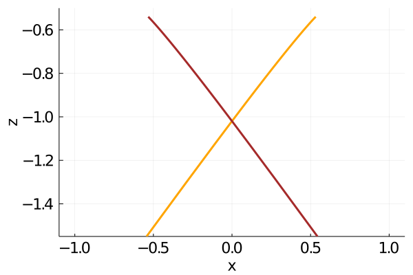
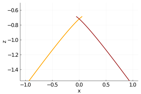
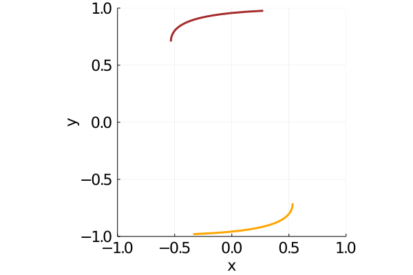
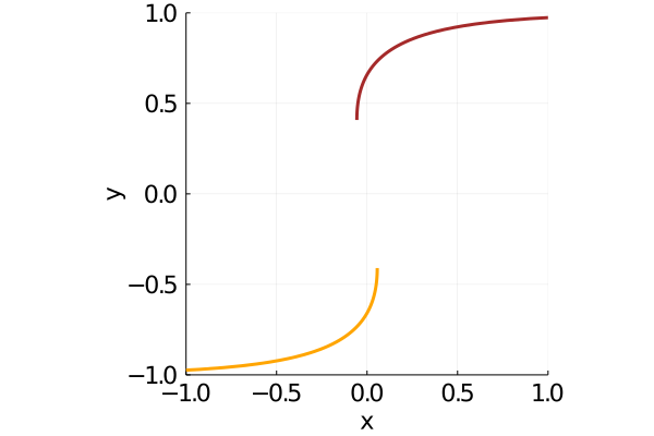
Figure 11: Pruned projections of the Legendre submanifold generated by $\psi_{\,J_{\,0}}(x,y)$ onto the $(x,y)$- and $(x,z)$-planes. These were depicted with the use of (21) by varying the value of $y$ in $(-1,1)$, and pruning the middle segments. Such middle parts on the $(x,y)$-plane are from $(x(y_{\,\mu\,-}^{\,*}),y_{\,\mu\,-}^{\,*})$ to $(x(y_{\,\mu\,+}^{\,*}),y_{\,\mu\,+}^{\,*})$, where $y_{\,\mu\,\pm}^{\,*}$ and $x$ as a function of $y$ have been defined in (25) and (21), respectively. The curves expressing lower values of $y$ in the lower panels of the left and right figures correspond to the curves of the shape of $/$ in the upper panels. (Left) Far from the critical point in the low temperature phase ($J_{\,0}=1.0$ in the dimensionless variable constructed from $\beta=1.0$ and $J_{\,0}=1.0$ in the dimensional variables). (Right) Near the critical point in the low temperature phase ($J_{\,0}=0.6$ in the dimensionless variable, obtained from $\beta=0.6$ and $J_{\,0}=1.0$ as the dimensional variables).

Singularities associated with the phase transition with respect to the external field do not appear in the $1$-dimensional Legendre submanifold $\phi{\cal A}$ embedded in the $3$-dimensional contact manifold. To verify this, first recall that in general a singular point of a curve is a point where its tangent vector vanishes. Second, focus on the curve as the Legendre submanifold $\gamma_{\,xyz}:\Upsilon\to\phi{\cal A}$, ($y\mapsto(x(y),y,z(y))$), where $y$ is the abbreviation of $y_{\,\mu}^{\,*}$ and $z(y)=\psi_{\,J_{0}}(x(y),y)$. Then calculate the tangent vector along $\gamma_{\,xyz}$, from which one has

$$\gamma_{\,xyz\,*}\left(\frac{\mathrm{d}}{\mathrm{d}y}\right) = \frac{\mathrm{d}x}{\mathrm{d}y}\frac{\partial}{\partial x}+\frac{\partial}{\partial y}+\frac{\mathrm{d}z}{\mathrm{d}y}\frac{\partial}{\partial z}\qquad=\frac{\mathrm{d}x}{\mathrm{d}y}\frac{\partial}{\partial x}+\frac{\partial}{\partial y}+\left(\frac{\partial z}{\partial y}+\frac{\partial z}{\partial x}\frac{\mathrm{d}x}{\mathrm{d}y}\right)\frac{\partial}{\partial z}$$

$$= \left(-2J_{\,0}+\frac{1}{1-y^{\,2}}\right)\frac{\partial}{\partial x}+\frac{\partial}{\partial y}+\left(-2J_{\,0}+\frac{1}{1-y^{\,2}}\right)\frac{\partial\psi_{\,J_{0}}}{\partial x}\frac{\partial}{\partial z}\neq 0,\quad\mbox{at any point of $y\in\Upsilon$,}$$

where (20), (23), (24) have been used, and $\gamma_{\,xyz\,*}$ is the push-forward of $\gamma_{\,xyz}$. Thus, there is no singular point on the Legendre curve. Meanwhile such singularities appear on the $(x,z)$-plane as the result of the projection. To show this, one calculates the tangent vector of the curve $\gamma_{\,xz}:\Upsilon\to\mathbb{R}\times\mathbb{R}$, ($y\mapsto(x(y),z(y))$),

$$\gamma_{\,xz\,*}\left(\frac{\mathrm{d}}{\mathrm{d}y}\right) = \frac{\mathrm{d}x}{\mathrm{d}y}\frac{\partial}{\partial x}+\frac{\mathrm{d}z}{\mathrm{d}y}\frac{\partial}{\partial z}$$

$$= \left(-2J_{\,0}+\frac{1}{1-y^{\,2}}\right)\frac{\partial}{\partial x}+\left(-2J_{\,0}+\frac{1}{1-y^{\,2}}\right)\frac{\partial\psi_{\,J_{0}}}{\partial x}\frac{\partial}{\partial z}.$$

From this calculation and (25), one verifies that there are singular points at the spinodal points, $y_{\,\mu\,\pm}^{\,*}$.

3.2 Nonequilibrium

Nonequilibrium processes are time-dependent thermodynamic processes, and their geometric descriptions have been proposed in the literature. There are a variety of classes of nonequilibrium states, and our nonequilibrium thermodynamic states are such that thermodynamic variables can uniquely specify thermodynamic states. In the contact geometric framework, such a description of a thermodynamic process is to choose a suitable contact Hamiltonian system. Among various nonequilibrium thermodynamic processes, relaxation processes have mainly been investigated, where such a process describes a time-development of a state towards the most stable equilibrium state. In this section, an appropriate contact Hamiltonian is introduced for describing the dynamical process from metastable equilibrium states to the most stable equilibrium ones.

We focus on the low temperature phase (symmetry broken phase), since the system in the high temperature phase is equivalent to systems with no-phase transitions and has been addressed [12]. To discuss system in Fig. 11, label branches of the $2$-valued function of $x$ as in Fig. 12 (left, low temperature phase), where the function $\psi_{\,J_{0}}$ does not depend on $y$ on the Legendre submanifold due to (23) with (22). Then, on the Legendre submanifold generated by $\psi_{\,J_{0}}$, the abbreviation $\psi_{\,\mu}(x)=\psi_{\,J_{0}}(x,y_{\,\mu}^{\,*})$ is introduced for each $\mu$. The region ${\cal I}^{\,+}\subset\mathbb{R}_{\,>0}$ is defined such that there are two (single-valued) functions, in particular $\psi_{\,1}$ and $\psi_{\,2}$ are labeled such that $\psi_{\,1}(x)<\psi_{\,2}(x)$, $(x\in{\cal I}^{\,+})$. That is, ${\cal I}^{\,+}:=\{\,x\in\mathbb{R}_{\,>0}\,|\,\psi_{\,1}(x)<\psi_{\,2}(x)\,\}$, (see Figs. 2 and 12). In the high temperature phase, the (single-valued) function appears. Then, decompose the subset of the Legendre submanifold $\phi{\cal A}_{\,\psi_{\,J_{0}}}$ into the ones with ${\cal I}^{\,+}$

$$\phi{\cal A}_{\,\mu}^{\,{\cal I}^{\,+}}=\left\{\ (x,y,z)\in{\cal C}\ \bigg{|}\ y=-\,\frac{\mathrm{d}\psi_{\,\mu}}{\mathrm{d}x},\ z=\psi_{\,\mu}(x),\quad x\in{\cal I}^{\,+}\ \right\},\quad\mu=1,2.$$

Figure 12: Wave front. (Left) Low temperature phase. The label $\mu$ for $\psi_{\,\mu}$ is chosen so that $\psi_{\,1}(x)<\psi_{\,2}(x)$. (Right) High temperature phase, the (single-valued) function appears.

One then can show the main theorem of this paper as below. Notice that no explicit expression of $\psi_{\,\mu}$ defined on ${\cal I}^{\,+}$ is needed for each $\mu$. Other different Theorems closely related to this main theorem are stated in Appendix A.

Theorem 3.1.

(satable segments of the hysteresis curve in the symmetry broken phase). On the thermodynamic phase space for the Husimi-Temperley model, choose a contact Hamiltonian $h$ as

$$h(x,z)=-\psi_{\,0}(x)(z-\psi_{\,1}(x))(z-\psi_{\,2}(x))^{\,2},$$ (26)

where $\psi_{\,0}$ is an arbitrary function of $x$ such that $\psi_{\,0}(x)>0$. Then the following hold.

1. The space $\phi{\cal A}_{\,1}^{\,{\cal I}^{\,+}}$ is asymptotically stable in ${\cal D}_{\,1}^{\,+}$, where

   $${\cal D}_{\,1}^{\,+}=\{\ (x,y,z)\ |\ x\in{\cal I}^{\,+},\ z<\psi_{\,2}(x)\ \}.$$

2. The space $\phi{\cal A}_{\,2}^{\,{\cal I}^{\,+}}$ is asymptotically stable in ${\cal D}_{\,2}^{\,+}$, where

   $${\cal D}_{\,2}^{\,+}=\{\ (x,y,z)\ |\ x\in{\cal I}^{\,+},\ \psi_{\,2}(x)\leq z\ \}.$$

Proof.

Our strategy for proving this is to show the existence of Lyapunov functions [50] for the dynamical system, where this dynamical system is obtained from substituting the contact Hamiltonian (26) into (3). The details are as follows.

First, a point of departure for this proof is to express the explicit form of the dynamical system written in terms of the coordinates $(x,y,z)$. From (3) and (26), the dynamical system is explicitly written as

$$\dot{x} = 0,$$ (27)

$$\dot{y} = \frac{\mathrm{d}\psi_{\,0}}{\mathrm{d}x}(z-\psi_{\,1})(z-\psi_{\,2})^{\,2}-\psi_{\,0}\left(y+\frac{\mathrm{d}\psi_{\,1}}{\mathrm{d}x}\right)(z-\psi_{\,2})^{\,2}-2\psi_{\,0}\left(y+\frac{\mathrm{d}\psi_{\,2}}{\mathrm{d}x}\right)(z-\psi_{\,1})(z-\psi_{\,2}),$$ (28)

$$\dot{z} = h=-\,\psi_{\,0}(x)(z-\psi_{\,1}(x))(z-\psi_{\,2}(x))^{\,2}.$$ (29)

The next step is to find fixed point sets. From

$$\dot{x}|_{\,\phi{\cal A}_{\mu}^{{\cal I}^{+}}}=0,\quad\dot{y}|_{\,\phi{\cal A}_{\mu}^{{\cal I}^{+}}}=0,\quad\dot{z}|_{\,\phi{\cal A}_{\mu}^{{\cal I}^{+}}}=0,\qquad\mu=1,2$$

one has that $\phi{\cal A}_{\,\mu}^{{\cal I}^{+}}\subset{\cal C}$, $(\mu=1,2)$ forms a fixed point set for each $\mu$. Here a phase portrait of the dynamical system is roughly discussed. It follows from (27) that $x$ is constant in time, and thus $\psi_{\,\mu}(x)$ does not depend on time.

Third, to prove the theorem, Lyapunov functions are constructed [50]. Define the functions $V_{\,1}$ on ${\cal D}_{\,1}^{\,+}$, and $V_{\,2}$ on ${\cal D}_{\,2}^{\,+}$, such that

$$V_{\,1}(x,z) = \frac{1}{2}(z-\psi_{\,1}(x))^{\,2},\qquad(x,y,z)\in{\cal D}_{\,1}^{\,+},$$

$$V_{\,2}(x,z) = z-\psi_{\,2}(x),\qquad(x,y,z)\in{\cal D}_{\,2}^{\,+}.$$

Then, differentiation of $V_{1}$ and that of $V_{2}$ yield the following.

• It follows that

  $$V_{\,1}(x,z)\geq 0,\quad\frac{\mathrm{d}V_{\,1}}{\mathrm{d}t}=(z-\psi_{\,1})h(x,z)=-\,\psi_{\,0}(x)(z-\psi_{\,1})^{\,2}(z-\psi_{\,2})^{\,2}\leq 0,\qquad(x,y,z)\in{\cal D}_{\,1}^{\,+},$$

  where the equality holds on the fixed point set $\phi{\cal A}_{\,1}^{\,{\cal I}^{\,+}}$. Hence $V_{\,1}$ is a Lyapunov function on ${\cal D}_{\,1}^{\,+}$.

• It follows that

  $$V_{\,2}(x,z)\geq 0,\quad\frac{\mathrm{d}V_{\,2}}{\mathrm{d}t}=h(x,z)=-\,\psi_{\,0}(x)(z-\psi_{\,1})(z-\psi_{\,2})^{\,2}\leq 0,\qquad(x,y,z)\in{\cal D}_{\,2}^{\,+},$$

  where the equality holds on the fixed point set $\phi{\cal A}_{\,2}^{\,{\cal I}^{\,+}}$. Hence $V_{\,2}$ is a Lyapunov function on ${\cal D}_{\,2}^{\,+}$.

According to the theorem of Lyapunov, one completes the proof. ∎

Theorem 3.1 shows that the proposed contact Hamiltonian vector field is such that the pruned segments of the projected Legendre submanifold are stable in regions of a contact manifold. The global behavior for $z$ is understood from Fig. 13. One then deduces from Fig. 13 that, given $x$, $\lim_{t\to\infty}z(t)=\psi_{\,1}(x)$ in ${\cal D}_{\,1}^{\,+}$, and that $\lim_{t\to\infty}z(t)=\psi_{\,2}(x)$ in ${\cal D}_{\,2}^{\,+}$. If initial states are near $\phi{\cal A}_{\,2}^{\,+}$ in ${\cal D}_{\,1}^{\,+}$, then the integral curves connect metastable states and the most stable states. Meanwhile, in the case where there is only one (single-valued) function $\psi$ of $x$ defined on a region in $\mathbb{R}$, one can find a contact Hamiltonian system such that the projection of the Legendre submanifold is stable as has been argued in Refs. [12, 25].

Figure 13: Phase space of the dynamical system consisting of $\dot{z}=h(x,z)$ and $\dot{x}=0$ ((29) and (27), respectively). From $\dot{z}=h$, it follows that the zeros of $h$ are the fixed points. From $h$ in (26) its zeros are the set $z=\psi_{\,1}(x)$ and the set $z=\psi_{\,2}(x)$. In addition, from the sign of $h$, it follows that the set $z=\psi_{\,1}(x)$ is stable in ${\cal D}_{\,1}^{\,+}$ and that the set $z=\psi_{\,2}(x)$ is stable in ${\cal D}_{\,2}^{\,+}$.

Physically, the contact Hamiltonian vector field with (26) expresses the dynamical process towards equilibrium states when initial states are not at equilibrium.

To grasp local flow around the fixed point set $(y_{\,1},z_{\,1})=(-\psi_{\,1}^{\,\prime},\psi_{\,1})$, the integral curves of the linearized equations are shown below. For the point $(y_{\,1},z_{\,1})=(-\psi_{\,1}^{\,\prime},\psi_{\,1})$, introduce $Y_{\,1}$ and $Z_{\,1}$ such that

$$y(t)=-\psi_{\,1}^{\,\prime}(x)+Y_{\,1}(t),\quad z(t)=\psi_{\,1}(x)+Z_{\,1}(t),\quad\mbox{where}\quad\psi_{\,1}^{\,\prime}(x):=\frac{\mathrm{d}\psi_{\,1}}{\mathrm{d}x}(x),$$

which yield linearized equations. For ease of notation, introduce

$$\psi_{\,21}(x)=\psi_{\,2}(x)-\psi_{\,1}(x)\ >0,$$ (30)

for each point $x$. Then the linearized equations are obtained as

$$\dot{Z}_{\,1}=-\,\underbrace{\psi_{\,0}\,\psi_{\,21}^{\ 2}}_{>\ 0}\,Z_{\,1},\qquad\dot{Y}_{\,1}=-\underbrace{\psi_{\,0}\,\psi_{\,21}^{\ 2}}_{>\ 0}\,Y_{\,1}+(\,\psi_{\,0}^{\,\prime}\,\psi_{\,21}^{\ 2}+\psi_{\,0}\,\psi_{\,21}\,\psi_{\,21}^{\,\prime}\,)\,Z_{\,1},$$

where $\psi_{\,21}^{\,\prime}(x)=\mathrm{d}\psi_{\,21}/\mathrm{d}x$ and $\psi_{\,0}^{\,\prime}=\mathrm{d}\psi_{\,0}/\mathrm{d}x$ are constants in time. To solve this linear system of equations, letting $c_{\,1}$ and $d_{\,1}$ be the constants such that

$$c_{\,1}=\psi_{\,0}\,\psi_{\,21}^{\ 2},\qquad d_{\,1}=\psi_{\,0}^{\,\prime}\,\psi_{\,21}^{\ 2}+\psi_{\,0}\,\psi_{\,21}\,\psi_{\,21}^{\,\prime},$$

one can write

$$\dot{Z}_{\,1}=-\,c_{\,1}Z_{\,1},\quad\dot{Y}_{\,1}=-\,c_{\,1}Y_{\,1}+d_{\,1}Z_{\,1},$$

The solution of this system is

$$Z_{\,1}(t)=Z_{\,1}(0)\,\mathrm{e}^{\,-c_{1}\,t},\quad Y_{\,1}(t)=(\,Y_{\,1}(0)+d_{\,1}Z_{\,1}(0)\,t\,)\,\mathrm{e}^{\,-c_{1}\,t}.$$

From this solution and the inequality $c_{\,1}>0$, one has that the fixed point set $\phi{\cal A}_{\,1}^{{\cal I}^{\,+}}$ is linearly stable. Observe from (30) that the strength of stability is large when the value $c_{\,1}=\psi_{\,0}\,\psi_{\,21}^{\,2}$ is large. The condition when $\psi_{\,21}(x)$ is large can be read off from Fig. 11. The value $\psi_{\,21}(x)$ is small near the critical point, and it is large far from the critical point.

So far the phase space ${\cal D}_{\,1}^{\,+}\cup{\cal D}_{\,2}^{\,+}$ of the dynamical system is focused, and then a similar claim can be stated for the region ${\cal D}_{\,1}^{\,-}\cup{\cal D}_{\,2}^{\,-}$, where ${\cal D}_{\,1}^{\,-}$ and ${\cal D}_{\,2}^{\,-}$ are defined with some ${\cal I}^{\,-}\subset\mathbb{R}_{<0}$. To state such a claim, introduce some notations as follows. Similar to the sets ${\cal D}_{\,1}^{\,+}=\{(x,y,z)\,|\,x\in{\cal I}^{\,+},z<\psi_{\,2}(x)\}$, and ${\cal I}^{\,+}=\{\,x\in\mathbb{R}_{\,>0}\,|\,\psi_{\,1}(x)<\psi_{\,2}(x)\,\}\subset\mathbb{R}$, introduce

$${\cal D}_{\,1}^{\,-}=\{(x,y,z)\ \,|\,x\in{\cal I}^{\,-},z<\psi_{\,2}(x)\},$$

where ${\cal I}^{\,-}$ has been defined in the caption to Fig. 2 as

$${\cal I}^{\,-}=\{\,x\in\mathbb{R}_{\,<0}\,|\,\psi_{\,1}(x)<\psi_{\,2}(x)\,\}\subset\mathbb{R}.$$

By combining these and refining it, one has the following.

Corollary 3.1.

(reconstruction of the stability of the hysteresis and pseudo-free energy curves as the Legendre submanifold). Consider the system shown in Fig. 10. In the joined region ${\cal D}_{\,1}^{\,+}\cup{\cal D}_{\,1}^{\,-}$ in the contact manifold ${\cal C}$, one has the contact Hamiltonian vector fields where the undirected curves $\overline{\mathrm{0-i}}$ and $\overline{\mathrm{v-vi}}$ are stable fixed point sets for $z<\psi_{\,2}$, and $\overline{\mathrm{i-ii}}$ and $\overline{\mathrm{iv-v}}$ are stable fixed point sets of the curve for $\psi_{\,2}\leq z$.

Notice that the $(y,z)$-plane at $x=0$ has been removed from ${\cal C}$ in Corollary 3.1. On this removed plane, the double-valued function becomes a single valued function, and thus the present contact Hamiltonian is not relevant. In addition, even if the segment $\overline{\mathrm{ii-iv}}$ is unremoved in Fig. 10, flows of the contact Hamiltonian system are not affected by the existence of the segment $\overline{\mathrm{ii-iv}}$.

In Fig. 14, the projected contact Hamiltonian vector fields stated in Corollary 3.1 are shown. From this corollary, one has the following.

Remark 3.1.

1. The cusp of the shape $\wedge$ on the $(x,z)$-plane is obtained in the long-time limit of the time-development of the contact Hamiltonian system, where such a shape is expected to be observed in experiments under perturbation.

2. The kink structure of the shape $\lrcorner\ulcorner$ on the $(x,y)$-plane is obtained in the long-time limit of the time-development of the contact Hamiltonian system, where such a kink shape is expected to be observed in experiments under perturbation.

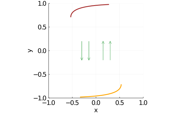
Figure 14: Projected contact Hamiltonian vector fields stated in Corollary 3.1, where the values of $\beta$ and $J_{\,0}$ were chosen to express a thermodynamic phase space being far from the critical point in the low temperature phase ($J_{\,0}=1.0$ in the dimensionless variable constructed from $\beta=1.0$ and $J_{\,0}=1.0$ in the dimensional variables). The pruned segments of the projections of the Legendre submanifold are stable and unstable fixed point sets. (Left) The $(x,z)$-plane. (Right) The $(x,y)$-plane.

4 Discussions and conclusions

This paper offers a contact geometric approach to thermodynamic systems that exhibit a phase transition. One key in this paper has been that the set of metastable, unstable, and the most stable equilibrium states is identified with a Legendre submanifold whose projections form multi-valued functions. As the main theorem of this paper unstable and stable segments of a hysteresis curve have been described as unstable and stable fixed point sets for a contact Hamiltonian vector field. Simultaneously the pseudo-free energy curve has also been described similarly, where this simultaneity is ascribed to the different projections of the unique Legendre submanifold. On this $1$-dimensional Legendre submanifold there is no singularity even in the symmetry broken phase. Meanwhile there are singularities on the $2$-dimensional plane as the result of the projection. Although these calculations have been for the so-called Husimi-Temperley model, calculations for other models and those for the present model are expected to be similar. The series of calculations has been summarized as a procedure, and then this procedure has been summarized in Introduction of this paper. A significance of this study is to provide a unified geometric manner in which a contact Hamiltonian and a single Legendre submanifold together with an associated pruning process lead to various notions and tools in thermodynamics. Such notions and tools are non-most-stable and most stable equilibrium states, hysteresis and pseudo-free energy curves, and rules similar to the Maxwell construction and the convexification.

There remain unsolved problems that have not been addressed in this paper. They include the following:

• derivation of the contact Hamiltonian vector field from a dynamical system that describes microscopic spins [40],

• application of the present approach to various statistical mechanical models, thermodynamic systems, and electric circuits [17],

• extension of the present or similar analysis to high-dimensional systems, rather than the present $3$-dimensional contact manifold,

• application of Legendre singularity and cobordism theories intensively to thermodynamic systems [46, 51],

• clarification of the relation between a contact version of the (graph) selector [52, 53] and the pruning introduced in this paper.

By addressing these, it is expected that a relevant and sophisticated geometric methodology will be established for dealing with various intricate systems and critical phenomena.

Data Availability Statement

In this paper various numerical figures have been drawn with the Julia language on a personal computer. To draw these figures, numerical plots have been made with elementary functions, including $\log$, $\tanh$, and so on. Hence there is no raw data, and these figures are easily reproduced. For this reason, data sharing is not applicable to this article as no new data were created or analyzed in this study.

Appendix A Appendix: Various contact Hamiltonian systems

For the sake of completeness, a system with the unpruned projection of the Legendre submanifold is argued in this section. In addition, a system similar to that in Theorem 3.1 is considered, and then it is shown that in $z>\psi_{\,2}$ the Legendre submanifold $\phi{\cal A}_{\,2}^{\,{\cal I}^{\,+}}$ forms a fixed point set but is unstable. Several contact Hamiltonian systems are considered in the main text and Appendix in this paper. They are summarized in Table 1. From a physical viewpoint, in Theorem A.1, one unsatisfactory feature is that $\phi{\cal A}_{\,3}^{\,{\cal I}^{+}}$ is stable, and another one is that the (meta-)stability of $\phi{\cal A}_{\,2}^{\,+}$ is lost. In addition, in Theorem A.2, one unsatisfactory feature is that the (meta-)stability of $\phi{\cal A}_{\,2}^{\,{\cal I}^{+}}$ is lost.

Theorem	Contact Hamiltonian $h$	Graph of $h$	Stable fixed point sets
3.1	$h=-\psi_{\,0}(z-\psi_{\,1})(z-\psi_{\,2})^{\,2}$	Fig. 13	$\phi{\cal A}_{\,1}^{\,{\cal I}^{+}}$ in ${\cal D}_{\,1}^{\,+}$, and $\phi{\cal A}_{\,2}^{\,{\cal I}^{+}}$ in ${\cal D}_{\,2}^{\,+}$
A.1	$h=-\psi_{\,0}(z-\psi_{\,1})(z-\psi_{\,2})(z-\psi_{\,3})$	Fig. 16	$\phi{\cal A}_{\,1}^{\,{\cal I}^{+}}$ in ${\cal D}_{\,1}^{\,+}$, and $\phi{\cal A}_{\,3}^{\,{\cal I}^{+}}$ in ${\cal D}_{\,3}^{\,+}$
A.2	$h=\ \ \psi_{\,0}(z-\psi_{\,1})(z-\psi_{\,2})$	Fig. 17	$\phi{\cal A}_{\,1}^{\,{\cal I}^{+}}$ in ${\cal D}_{\,1}^{\,+}$

Table 1: Various contact Hamiltonian systems

A.1 Three branch system

To discuss system in Fig. 8, label branches of the $3$-valued function of $x$ as in Fig. 15 (left, low temperature phase), where the function $\psi_{\,J_{0}}$ does not depend on $y$ on the Legendre submanifold due to (23) with (22). Then, as in the case of Section 3.2, on the Legendre submanifold generated by $\psi_{\,J_{0}}$, the abbreviation $\psi_{\,\mu}(x)=\psi_{\,J_{0}}(x,y_{\,\mu}^{\,*})$ is introduced for each $\mu$. In the region ${\cal I}^{\,+}\subset\mathbb{R}$, there are three (single-valued) functions $\psi_{\,1},\psi_{\,2},\psi_{\,3}$ labeled such that $\psi_{\,1}(x)<\psi_{\,2}(x)<\psi_{\,3}(x)$, $(x\in{\cal I}^{\,+})$. In the high temperature phase, the (single-valued) function appears.

Figure 15: Wave front. (Left) Low temperature phase. The label $\mu$ for $\psi_{\,\mu}$ is chosen so that $\psi_{\,1}(x)<\psi_{\,2}(x)<\psi_{\,3}(x)$. (Right) High temperature phase, the (single-valued) function appears.

We focus on the low temperature phase again as in the case of the $2$-valued function. To discuss the low temperature phase, decompose the subset of the Legendre submanifold $\phi{\cal A}_{\,\psi_{\,J_{0}}}$ into the ones with ${\cal I}^{\,+}$

$$\phi{\cal A}_{\,\mu}^{\,{\cal I}^{+}}=\left\{\ (x,y,z)\ \bigg{|}\ y=-\,\frac{\mathrm{d}\psi_{\,\mu}}{\mathrm{d}x},\ z=\psi_{\,\mu}(x),\quad x\in{\cal I}^{\,+}\ \right\},\quad\mu=1,2,3.$$

One can show the following theorem. Notice, as well as in Theorem 3.1, that no explicit expression of $\psi_{\,\mu}$ defined on ${\cal I}^{\,+}$ is needed for each $\mu$.

Theorem A.1.

(stable and unstable segments of the hysteresis curve in the symmetry broken phase). On the thermodynamic phase space for the Husimi-Temperley model, choose a contact Hamiltonian $h$ as

$$h(x,z)=-\psi_{\,0}(x)(z-\psi_{\,1}(x))(z-\psi_{\,2}(x))(z-\psi_{\,3}(x)).$$ (A.1)

where $\psi_{\,0}$ is an arbitrary function of $x$ such that $\psi_{\,0}(x)>0$. Then the following hold.

1. The space $\phi{\cal A}_{\,1}^{\,{\cal I}^{+}}$ is asymptotically stable in ${\cal D}_{\,1}^{+}$, where

   $${\cal D}_{\,1}^{\,+}=\{\ (x,y,z)\ |\ x\in{\cal I}^{\,+},\ z<\psi_{\,2}(x)\ \}.$$

2. The space $\phi{\cal A}_{\,3}^{\,{\cal I}^{+}}$ is asymptotically stable in ${\cal D}_{\,3}^{+}$, where

   $${\cal D}_{\,3}^{\,+}=\{\ (x,y,z)\ |\ x\in{\cal I}^{\,+},\ z>\psi_{\,2}(x)\ \}.$$

Proof.

Our strategy for proving this is to show the existence of a Lyapunov function [50] for the dynamical system obtained from substituting the contact Hamiltonian (A.1) into (3). The details are as follows.

First, a point of departure for this proof is to express the explicit form of the dynamical system written in terms of the coordinates $(x,y,z)$. From (3) and (A.1), the dynamical system is explicitly written as

$$\dot{x} = 0,$$ (A.2)

$$\dot{y} = \frac{\mathrm{d}\psi_{\,0}}{\mathrm{d}x}(z-\psi_{\,1})(z-\psi_{\,2})(z-\psi_{\,3})-\psi_{\,0}\left(y+\frac{\mathrm{d}\psi_{\,1}}{\mathrm{d}x}\right)(z-\psi_{\,2})(z-\psi_{\,3})$$ (A.3)

$$-\psi_{\,0}\left(y+\frac{\mathrm{d}\psi_{\,2}}{\mathrm{d}x}\right)(z-\psi_{\,1})(z-\psi_{\,3})-\psi_{\,0}\left(y+\frac{\mathrm{d}\psi_{\,3}}{\mathrm{d}x}\right)(z-\psi_{\,1})(z-\psi_{\,2})$$

$$\dot{z} = h=-\,\psi_{\,0}(x)(z-\psi_{\,1}(x))(z-\psi_{\,2}(x))(z-\psi_{\,3}(x)).$$ (A.4)

The next step is to find fixed point sets. From

$$\dot{x}|_{\,\phi{\cal A}_{\mu}^{\,{\cal I}^{+}}}=0,\quad\dot{y}|_{\,\phi{\cal A}_{\mu}^{\,{\cal I}{+}}}=0,\quad\dot{z}|_{\,\phi{\cal A}_{\mu}^{\,{\cal I}^{+}}}=0.\qquad\mu=1,2,3$$

one has that $\phi{\cal A}_{\,\mu}^{\,{\cal I}^{+}}\subset{\cal C}$, $(\mu=1,2,3)$ forms a fixed point set for each $\mu$. Here a phase portrait of the dynamical system is roughly discussed. It follows from (A.2) that $x$ is constant in time, and thus $\psi_{\,\mu}(x)$ does not depend on time.

Third, to prove the theorem, Lyapunov functions are constructed  [50]. Define the functions $V_{\,1}$ in ${\cal D}_{\,1}^{\,+}$ and $V_{\,3}$ in ${\cal D}_{\,3}^{\,+}$ such that

$$V_{\,1}(x,z) = \frac{1}{2}(z-\psi_{\,1}(x))^{\,2},\qquad(x,y,z)\in{\cal D}_{\,1}^{\,+}$$

$$V_{\,3}(x,z) = \frac{1}{2}(z-\psi_{\,3}(x))^{\,2},\qquad(x,y,z)\in{\cal D}_{\,3}^{\,+}.$$

Then, differentiation of $V_{\,1}$ and that of $V_{\,3}$ yield the following.

• In ${\cal D}_{\,1}^{\,+}$, it follows that

  $$V_{\,1}(x,z)\geq 0,\quad\frac{\mathrm{d}V_{\,1}}{\mathrm{d}t}=(z-\psi_{\,1})h(x,z)=-\psi_{\,0}(z-\psi_{\,1})^{\,2}(z-\psi_{\,2})(z-\psi_{\,3})\leq 0,\qquad(x,y,z)\in{\cal D}_{\,1}^{\,+},$$

  where the equality holds on the fixed point set $\phi{\cal A}_{\,1}^{\,{\cal I}^{+}}$. Hence $V_{\,1}$ is a Lyapunov function in ${\cal D}_{\,1}^{\,+}$.

• In ${\cal D}_{\,3}^{\,+}$, it follows that

  $$V_{\,3}(x,z)\geq 0,\quad\frac{\mathrm{d}V_{\,3}}{\mathrm{d}t}=(z-\psi_{\,3})h(x,z)=-\psi_{\,0}(z-\psi_{\,1})(z-\psi_{\,2})(z-\psi_{\,3})^{\,2}\leq 0,\qquad(x,y,z)\in{\cal D}_{\,3}^{\,+},$$

  where equality holds on the fixed point set $\phi{\cal A}_{\,3}^{\,{\cal I}^{+}}$. Hence $V_{\,3}$ is a Lyapunov function in ${\cal D}_{\,3}^{\,+}$.

According to the theorem of Lyapunov, one completes the proof. ∎

The global behavior for $z$ is understood from Fig. 16. One then deduces from Fig. 16 that, given $x$, $\lim_{t\to\infty}z(t)=\psi_{\,1}(x)$ in ${\cal D}_{\,1}^{\,+}$, and that $\lim_{t\to\infty}z(t)=\psi_{\,3}(x)$ in ${\cal D}_{\,3}^{\,+}$.

Figure 16: Phase space of the dynamical system consisting of $\dot{z}=h(x,z)$ and $\dot{x}=0$ ((A.4) and (A.2)). From $\dot{z}=h$, it follows that the zeros of $h$ are the fixed points. From $h$ in (A.1) its zeros are the set $z=\psi_{\,1}(x)$, $z=\psi_{\,2}(x)$ and the set $z=\psi_{\,3}(x)$. In addition, from the sign of $h$, the set $z=\psi_{\,1}(x)$ and the set $z=\psi_{\,3}(x)$ are stable in some domains.

To elucidate the behavior of the contact Hamiltonian vector field in Theorem A.1 on the lower dimensional spaces that have been used for the projections, see Fig. 10. This Theorem states that $\phi{\cal A}_{\,1}^{\,{\cal I}^{+}}$ and $\phi{\cal A}_{\,3}^{\,{\cal I}^{+}}$ are stable. This is equivalent to say that the part of Legendre curves $\overline{\mathrm{v-vi}}$ and $\overline{\mathrm{ii-iii}}$ are stable in some domains. Although it is not immediately clear how the stability of the curve $\overline{\mathrm{ii-iii}}$ plays a role in physical context, the role of stability of the curve $\overline{\mathrm{v-vi}}$ is clear. That stability for $\overline{\mathrm{v-vi}}$ is consistent with the thermodynamic stability.

To grasp local flow around the fixed point sets, integral curves of the linearized equations are shown below. For the point $(y_{\mu},z_{\mu})=(-\psi_{\,\mu}^{\,\prime},\psi_{\,\mu})$, introduce $Y_{\,\mu}$ and $Z_{\,\mu}$ such that

$$y(t)=-\psi_{\,\mu}^{\,\prime}(x)+Y_{\,\mu}(t),\quad z(t)=\psi_{\,\mu}(x)+Z_{\,\mu}(t),\quad\mbox{where}\quad\psi_{\,\mu}^{\,\prime}(x):=\frac{\mathrm{d}\psi_{\,\mu}}{\mathrm{d}x}(x),\quad\mu=1,2,3$$

which yield linearized equations. For ease of notation, introduce

$$\psi_{\,\mu\mu^{\prime}}=\psi_{\,\mu}(x)-\psi_{\,\mu^{\prime}}(x),\quad\mu,\mu^{\,\prime}=1,2,3,\qquad\psi_{\,\mu\mu^{\prime}}>0,\quad\qquad(\mu>\mu^{\,\prime}).$$ (A.5)

Then the linearized equations are obtained as

$$\dot{Z}_{\,1}=-\,\underbrace{\psi_{\,0}\,\psi_{\,21}\psi_{\,31}}_{>\ 0}\,Z_{\,1},\qquad\dot{Z}_{\,2}=\ \ \underbrace{\psi_{\,0}\,\psi_{\,21}\psi_{\,32}}_{>\ 0}\,Z_{\,2},\qquad\dot{Z}_{\,3}=-\,\underbrace{\psi_{\,0}\psi_{\,31}\psi_{\,32}}_{>\ 0}\,Z_{\,3},$$ (A.6)

and

$$\dot{Y}_{\,1} = -\psi_{\,0}\,\psi_{\,21}\psi_{\,31}\,Y_{\,1}+(\,\psi_{\,0}^{\,\prime}\,\psi_{\,21}\,\psi_{\,31}+\psi_{\,0}\,\psi_{\,21}^{\,\prime}\,\psi_{\,31}+\psi_{\,0}\,\psi_{\,21}\,\psi_{\,31}^{\,\prime})\,Z_{\,1},$$

$$\dot{Y}_{\,2} = \ \psi_{\,0}\,\psi_{\,21}\psi_{\,32}\,Y_{\,2}-(\,\psi_{\,0}^{\,\prime}\,\psi_{\,21}\,\psi_{\,32}+\psi_{\,0}\,\psi_{\,21}^{\,\prime}\,\psi_{\,32}+\psi_{\,0}\,\psi_{\,21}\,\psi_{\,32}^{\,\prime})\,Z_{\,2},$$

$$\dot{Y}_{\,3} = -\psi_{\,0}\,\psi_{\,31}\psi_{\,32}\,Y_{\,3}+(\,\psi_{\,0}^{\,\prime}\,\psi_{\,31}\,\psi_{\,32}+\psi_{\,0}\,\psi_{\,31}^{\,\prime}\,\psi_{\,32}+\psi_{\,0}\,\psi_{\,31}\,\psi_{\,32}^{\,\prime})\,Z_{\,3}.$$

To solve this linear system of equations, letting $c_{\,\mu}$ and $d_{\,\mu}$ be some constants, one can write the system as

$$\dot{Z}_{\,\mu}=-\,c_{\,\mu}Z_{\,\mu},\quad\dot{Y}_{\,\mu}=-\,c_{\,\mu}Y_{\,\mu}+d_{\,\mu}Z_{\,\mu}.$$

The solution of this system is

$$Z_{\,\mu}(t)=Z_{\,\mu}(0)\,\mathrm{e}^{\,-c_{\mu}\,t},\quad Y_{\,\mu}(t)=(\,Y_{\,\mu}(0)+d_{\,\mu}Z_{\,\mu}(0)\,t\,)\,\mathrm{e}^{\,-c_{\mu}\,t}.$$

From this and the inequalities $c_{\,1}>0$, $c_{\,3}>0$, $c_{\,2}<0$, one has that the fixed point sets $\phi{\cal A}_{\,1}^{\,{\cal I}^{+}}$ and $\phi{\cal A}_{\,3}^{\,{\cal I}^{+}}$ are linearly stable, and the $\phi{\cal A}_{\,2}^{\,{\cal I}^{+}}$ is linearly unstable. Observe from (A.5) and (A.6) that the strength of instability/stability is large when the value $\psi_{\,\mu\mu^{\,\prime}}$ is large. The condition when $\psi_{\,\mu\mu^{\,\prime}}(x)$ is large can be read off from Fig. 8. The values $\psi_{\,\mu\mu^{\prime}}$ are small near the critical point, and they are large far from the critical point.

A.2 Two branch system

We focus on the low temperature phase again, and the following is about another contact Hamiltonian system.

Theorem A.2.

(stable segment of the hysteresis curve in the symmetry broken phase). On the thermodynamic phase space for the Husimi-Temperley model, choose a contact Hamiltonian $h$ as

$$h(x,z)=\psi_{\,0}(x)(z-\psi_{\,1}(x))(z-\psi_{\,2}(x)),$$ (A.7)

where $\psi_{\,0}$ is an arbitrary function of $x$ such that $\psi_{\,0}(x)>0$. Then the following holds.

1. The space $\phi{\cal A}_{\,1}^{\,{\cal I}^{\,+}}$ is asymptotically stable in ${\cal D}_{\,1}^{\,+}$, where

   $${\cal D}_{\,1}^{\,+}=\{\ (x,y,z)\ |\ x\in{\cal I}^{\,+},\ z<\psi_{\,2}(x)\ \}.$$

Proof.

Our strategy for proving this is to show the existence of a Lyapunov function [50] for the dynamical system, where this system is obtained from substituting the contact Hamiltonian (A.7) into (3). The details are as follows.

First, a point of departure for this proof is to express the explicit form of the dynamical system written in terms of the coordinates $(x,y,z)$. From (3) and (A.7), the dynamical system is explicitly written as

$$\dot{x} = 0,$$ (A.8)

$$\dot{y} = -\,\frac{\mathrm{d}\psi_{\,0}}{\mathrm{d}x}(z-\psi_{\,1})(z-\psi_{\,2})+\psi_{\,0}\left(y+\frac{\mathrm{d}\psi_{\,1}}{\mathrm{d}x}\right)(z-\psi_{\,2})+\psi_{\,0}\left(y+\frac{\mathrm{d}\psi_{\,2}}{\mathrm{d}x}\right)(z-\psi_{\,1})$$ (A.9)

$$\dot{z} = h=\psi_{\,0}(x)(z-\psi_{\,1}(x))(z-\psi_{\,2}(x)).$$ (A.10)

The next step is to find fixed point sets. From

$$\dot{x}|_{\,\phi{\cal A}_{\mu}^{{\cal I}^{+}}}=0,\quad\dot{y}|_{\,\phi{\cal A}_{\mu}^{{\cal I}^{+}}}=0,\quad\dot{z}|_{\,\phi{\cal A}_{\mu}^{{\cal I}^{+}}}=0,\qquad\mu=1,2$$

one has that $\phi{\cal A}_{\,\mu}^{{\cal I}^{+}}\subset{\cal C}$, $(\mu=1,2)$ forms a fixed point set for each $\mu$. Here a phase portrait of the dynamical system is roughly discussed. It follows from (A.8) that $x$ is constant in time, and thus $\psi_{\,\mu}(x)$ does not depend on time.

Third, to prove the theorem, a Lyapunov function is constructed [50]. Define the function $V_{\,1}$ in ${\cal D}_{\,1}^{\,+}$ such that

$$V_{\,1}(x,z)=\frac{1}{2}(z-\psi_{\,1}(x))^{\,2},\qquad(x,y,z)\in{\cal D}_{\,1}^{\,+}.$$

Then, it follows that

$$V_{\,1}(x,z)\geq 0,\quad\frac{\mathrm{d}V_{\,1}}{\mathrm{d}t}=(z-\psi_{\,1})h(x,z)=\psi_{\,0}(z-\psi_{\,1})^{\,2}(z-\psi_{\,2})\leq 0,\qquad(x,y,z)\in{\cal D}_{\,1}^{\,+},$$

where the equality holds on the fixed point set $\phi{\cal A}_{\,1}^{\,{\cal I}^{\,+}}$. Hence $V_{\,1}$ is a Lyapunov function in ${\cal D}_{\,1}^{\,+}$. According to the theorem of Lyapunov, one completes the proof. ∎

Theorem A.2 shows that the proposed contact Hamiltonian vector field is such that a segment of the projected Legendre submanifold is stable in a region of a contact manifold. The global behavior for $z$ is understood from Fig. 17. One then deduces from Fig. 17 that, given $x$, $\lim_{t\to\infty}z(t)=\psi_{\,1}(x)$ in ${\cal D}_{\,1}^{\,+}$.

Figure 17: Phase space of the dynamical system consisting of $\dot{z}=h(x,z)$ and $\dot{x}=0$ ((A.10) and (A.8), respectively). From $\dot{z}=h$, it follows that the zeros of $h$ are the fixed points. From $h$ in (A.7) its zeros are the set $z=\psi_{\,1}(x)$ and the set $z=\psi_{\,2}(x)$. In addition, from the sign of $h$, it follows that the set $z=\psi_{\,1}(x)$ is stable in ${\cal D}_{\,1}^{\,+}$.

Physically, the contact Hamiltonian vector field with (A.7) expresses the dynamical process departing from initial states in ${\cal D}_{\,1}^{\,+}$ to the most stable equilibrium ones.

To grasp local flow around the fixed point sets, the integral curves of the linearized equations are shown below. For the point $(y_{\mu},z_{\mu})=(-\psi_{\,\mu}^{\,\prime},\psi_{\,\mu})$, introduce $Y_{\,\mu}$ and $Z_{\,\mu}$ such that

$$y(t)=-\psi_{\,\mu}^{\,\prime}(x)+Y_{\,\mu}(t),\quad z(t)=\psi_{\,\mu}(x)+Z_{\,\mu}(t),\quad\mbox{where}\quad\psi_{\,\mu}^{\,\prime}(x):=\frac{\mathrm{d}\psi_{\,\mu}}{\mathrm{d}x}(x),\quad\mu=1,2$$

which yield linearized equations. For ease of notation, introduce

$$\psi_{\,21}(x)=\psi_{\,2}(x)-\psi_{\,1}(x)\ >0,\quad$$ (A.11)

for each point $x$. Then the linearized equations are obtained as

$$\dot{Z}_{\,1} = -\,\underbrace{\psi_{\,0}\,\psi_{\,21}}_{>\ 0}\,Z_{\,1},\qquad\dot{Z}_{\,2}=\ \ \underbrace{\psi_{\,0}\,\psi_{\,21}}_{>\ 0}\,Z_{\,2},$$

$$\dot{Y}_{\,1} = -\psi_{\,0}\,\psi_{\,21}\,Y_{\,1}+(\,\psi_{\,0}^{\,\prime}\,\psi_{\,21}+\psi_{\,0}\,\psi_{\,21}^{\,\prime}\,)\,Z_{\,1},\qquad\dot{Y}_{\,2}=\ \psi_{\,0}\,\psi_{\,21}\,Y_{\,2}-(\psi_{\,0}^{\,\prime}\,\psi_{\,21}+\psi_{\,0}\,\psi_{\,21}^{\,\prime}\,)\,Z_{\,2},$$

where $\psi_{\,21}^{\,\prime}(x)=\mathrm{d}\psi_{\,21}/\mathrm{d}x$ and $\psi_{\,0}^{\,\prime}=\mathrm{d}\psi_{\,0}/\mathrm{d}x$ that are constants in time. To solve this linear system of equations, letting $c_{\,\mu}$ and $d_{\,\mu}$ be the constants such that

$$c_{\,1}=\psi_{\,0}\,\psi_{\,21},\quad c_{\,2}=-\,c_{\,1},\qquad d_{\,1}=\psi_{\,0}^{\,\prime}\,\psi_{\,21}+\psi_{\,0}\,\psi_{\,21}^{\,\prime},\quad d_{\,2}=-d_{\,1},$$

one can write

$$\dot{Z}_{\,\mu}=-\,c_{\,\mu}Z_{\,\mu},\quad\dot{Y}_{\,\mu}=-\,c_{\,\mu}Y_{\,\mu}+d_{\,\mu}Z_{\,\mu},\quad\mu=1,2.$$

The solution of this system is

$$Z_{\,\mu}(t)=Z_{\,\mu}(0)\,\mathrm{e}^{\,-c_{\mu}\,t},\quad Y_{\,\mu}(t)=(\,Y_{\,\mu}(0)+d_{\,\mu}Z_{\,\mu}(0)\,t\,)\,\mathrm{e}^{\,-c_{\mu}\,t}.$$

From this, the inequalities $c_{\,1}>0$ and $c_{\,2}<0$, one has that the fixed point set $\phi{\cal A}_{\,1}^{{\cal I}^{\,+}}$ is linearly stable, and that the $\phi{\cal A}_{\,2}^{{\cal I}^{\,+}}$ linearly unstable. Observe from (A.11) that the strength of instability/stability is large when the value $c_{\,1}=\psi_{\,0}\,\psi_{\,21}$ is large. The condition when $\psi_{\,21}(x)$ is large can be read off from Fig. 11. The value $\psi_{\,21}(x)$ is small near the critical point, and it is large far from the critical point.

So far the phase space ${\cal D}_{\,1}^{\,+}$ of the dynamical system is focused, and then a similar claim can be stated for the region ${\cal D}_{\,1}^{\,-}$, where ${\cal D}_{\,1}^{\,-}$ is defined with some ${\cal I}^{\,-}\subset\mathbb{R}_{<0}$. To state such a claim, recall the following:

$${\cal D}_{\,1}^{\,+}=\{(x,y,z)\ |\,x\in{\cal I}^{\,+},z<\psi_{\,2}(x)\},\quad{\cal I}^{\,+}=\{\,x\in\mathbb{R}_{\,>0}\,|\,\psi_{\,1}(x)<\psi_{\,2}(x)\,\}\subset\mathbb{R},$$

and

$${\cal D}_{\,1}^{\,-}=\{(x,y,z)\ |\,x\in{\cal I}^{\,-},z<\psi_{\,2}(x)\},\quad{\cal I}^{\,-}=\{\,x\in\mathbb{R}_{\,<0}\,|\,\psi_{\,1}(x)<\psi_{\,2}(x)\,\}\subset\mathbb{R}.$$

By combining these and refining it, one has the following.

Corollary A.1.

(reconstruction of the stability of the hysteresis and pseudo-free energy curves as the Legendre submanifold). Consider the system shown in Fig. 10 with the curve $\overline{\mathrm{ii-iv}}$ being removed. In the joined region ${\cal D}_{\,1}^{\,+}\cup{\cal D}_{\,1}^{\,-}$ in the contact manifold ${\cal C}$, one has the contact Hamiltonian vector fields where the undirected curves $\overline{\mathrm{0-i}}$ and $\overline{\mathrm{v-vi}}$ are stable fixed point sets.

Notice that the $(y,z)$-plane at $x=0$ has been removed from ${\cal C}$ in Corollary A.1. On this removed plane, the double-valued function becomes a single valued function, and thus the present contact Hamiltonian is not relevant. The projected contact Hamiltonian vector fields stated in Corollary A.1 can be shown, and they are the same as Fig. 14. From this corollary, one has again Remark 3.1.

References

- [1] P. Libermann, and C-M. Marle, Symplectic Geometry and Analytical Mechanics, Springer, 1987
- [2] A. da Silva, Lectures on Symplectic Geometry, Springer, 2008
- [3] A. McInerney, First Steps in Differential Geometry, Springer, 2013
- [4] V.I. Arnold, Mathematical Methods of Classical Mechanics, Springer, 1976
- [5] H. Geiges, An Introduction to Contact Topology, Cambridge University Press, 2008
- [6] D.E. Blair, Contact Manifolds in Riemannian Geometry, Springer, 1976
- [7] K. Wang, L. Wang, and J. Yan, Aubry–Mather Theory for Contact Hamiltonian Systems, Comm. Math. Phys., 366, 981–1023, 2019
- [8] R. Harmann, Geometry, physic and systems, Dekker, 1973
- [9] R. Mrugala, On contact and metric structures on thermodynamic spaces, Suken kokyuroku, 1142, 167–181, 2000
- [10] R. Mrugala, J.D. Nulton, J.C. Schön, and P. Salamon, Statistical approach to the geometric structure of thermodynamics, Phys. Rev. A, 41, 3156–3160, 1990
- [11] A. Kushner, V. Lychagin, and M. Roop, Optimal Thermodynamic Processes For Gases, Entropy, 22, 448, 2020
- [12] S. Goto, Legendre submanifolds in contact manifolds as attractors and geometric nonequilibrium thermodynamics, J. Math. Phys., 56, 073301, 2015
- [13] A. Mori, Information geometry in a global setting, Hiroshima Math. J., 48, 291–305, 2018
- [14] N. Nakajima, and T. Ohmoto, The dually flat structure for singular models, Information Geometry, 2021
- [15] J. Etnyre, and R. Ghrist, Contact topology and hydrodynamics I: Beltrami fields and the Seifert conjecture, Nonlinearity, 13, 441–458, 2000
- [16] T. Ohsawa, Contact geometry of the Pontryagin maximum principle, Automatica, 55, 1–5, 2015
- [17] S. Goto, Contact geometric descriptions of vector fields on dually flat spaces and their applications in electric circuit models and nonequilibrium statistical mechanics J. Math. Phys., 57, 102702, 2016
- [18] A. Bravetti, M. Seri, M. Vermeeren, and F. Zadra, Numerical integration in Celestial Mechanics: a case for contact geometry, Celest. Mech. Dyn. Astr. 132, 2020
- [19] S. Goto, and H. Hino, Fast symplectic integrator for Nesterov-type acceleration method, arXiv:2106.07620
- [20] A. van der Schaft, and B. Maschke, Geometry of thermodynamic processes, Entropy , 20, 925, 2018
- [21] C.S. Lopez-Monsalvo, F. Nettel, V. Pineda-Reyes, and L.F. Escamilla-Herrera, Contact polarizations and associated metrics in geometric thermodynamics, J. Phys. A: Math. Theor., 54, 105202, 2021
- [22] J.F. Cariena, and P. Guha, Non-Standard Hamiltonian Structures of the Lienard Equation and Contact Geometry, Int. J. Geom. Methods Mod. Phys., 16, 1940001, 2019
- [23] A. Bravetti, H. Cruz, and D. Tapias, Contact Hamiltonian mechanics, Ann. Phys., 376, 17–39, 2017
- [24] M. de León and M.L. Valcazar, Contact Hamiltonian systems, J. Math. Phys., 60, 102902, 2019
- [25] M. Entov, and L. Polterovich, Contact topology and non-equilibirum thermodynamics, arXiv:2101.03770
- [26] T. Frenkel, The Geometry of Physics, 3rd edition, Cambridge University Press, 2011
- [27] M. Nakahara, Geometry, topology and physics, CRC press, 2003
- [28] R. Kubo, M. Toda, and N. Hashitsume, Statistical Physics II, Springer, 1991
- [29] M. Tuckerman, Statistical Mechanics: Theory and Molecular Simulation, Oxford University Press, 2010
- [30] S. Tasaki, Nonequilibrium stationary states of noninteracting electrons in a one-dimensional lattice, Chaos, Solitons and Fractals, 12, 2657-2674, 2001
- [31] C. Andrieu, et al, An Introduction to MCMC for Machine Learning, Machine Learning, 50, 5–43, 2003
- [32] T. Kita, Introduction to Nonequilibrium Statistical Mechanics with Quantum Field Theory, Prog. Theor. Phys., 123, 581–658, 2010
- [33] S. Goto, and H. Hino, Diffusion equations from master equations - A discrete geometric approach, J. Math. Phys., 61, 113301, 2020
- [34] D.N. Zubarev, V. Morozov, and G. Ropke, Statistical Mechanics of Nonequilibrium Processes, Volume 1 : Basic Concepts, Kinetic Theory, Wiley-VCH, 1996
- [35] D.N. Zubarev, V. Morozov, and G. Ropke, Statistical Mechanics of Nonequilibrium Processes, Volume 2 : Relaxation and Hydrodynamic Processes, Wiley-VCH, 1997
- [36] A. Campa, T. Dauxois, S. Ruffo, Statistical mechanics and dynamics of solvable models with long-range interactions, Physics Reports, 480, 57–159, 2009
- [37] I.D. Mayergoyz, Mathematical models of hysteresis, IEEE Trans. Magnetics, 22, 603–608, 1986
- [38] M. Toda, R. Kubo, and N, Saito, Statistical Physics, Springer, 1983
- [39] J.G. Brankov, and V.A. Zagrebnov, On the description of the phase transition in the Husimi-Temperley model, J. Phys. A: Math. Gen., 16 2217, 1983
- [40] T. Mori, S. Miyashita, and P.A. Rikvold, Asymptotic forms and scaling properties of the relaxation time near threshold points in spinodal-type dynamical phase transitions, Phys. Rev. E, 81, 011135, 2010
- [41] Y. Hashizume, and H. Matsueda, Information Geometry for Husimi-Temperley Model, arXiv:1407.2667
- [42] M. Grmela, Contact geometry of mesoscopic thermodynamics and dynamics, Entropy, 16, 1652–1686, 2014
- [43] H.W. Haslach, Geometric structure of the non-equilibrium thermodynamics of homogeneous systems, Rep. Math. Phys., 39, 147–162, 1997
- [44] H. Quevedo, A. Sanchez, S. Taj, and A. Vazquez, Phase transitions in geometrothermodynamics, Gen. Relative. Gravit., 43, 1135–1165, 2011
- [45] V.I. Arnold, Singularities of caustics and wave fronts, Springer, 1990
- [46] F. Aicardi, On the classification of singularities in thermodynamics, Physica D, 158, 175–196, 2001
- [47] F. Aicardi, P. Valentin, and E. Ferrand, On the classification of generic phenomena in one-parameter families of thermodynamic binary mixture, Phys. Chem. Chem. Phys., 4, 884–895, 2002
- [48] A. Shimizu, Principles of Thermodynamics, Tokyo University Press, In Japanese, 2007
- [49] H.B. Callen, Thermodynamics and an Introduction to Thermostatistics, 2nd Edition, Wiley, 1985
- [50] M. W. Hirsch and S. Smale, Differential Equations, Dynamical Systems, and Linear Algebra, Academic Press, 1974
- [51] V.I. Arnold and A.B. Givental, Symplectic geometry, Dynamical Systems IV, Symplectic Geometry and its Applications, edited by V.I. Arnold, and S. Novikov, Encyclopaedia of Mathematical Sciences 4, Springer, 1990
- [52] P. Gabriel, L. Polterovich, and K.F. Siburg, Boundary rigidity for Lagrangian submanifolds, non-removable intersections, and aubry-mather theory, Moscow Math. J., 3, 593–619, 2003
- [53] M. Limouzineau, Operations on Legendrian submanifolds, arXiv:1611.06823