Auxiliary-Classifier GAN for Malware Analysis

Abstract

Generative adversarial networks (GAN) are a class of powerful machine learning techniques, where both a generative and discriminative model are trained simultaneously. GANs have been used, for example, to successfully generate “deep fake” images. A recent trend in malware research consists of treating executables as images and employing image-based analysis techniques. In this research, we generate fake malware images using auxiliary classifier GANs (AC-GAN), and we consider the effectiveness of various techniques for classifying the resulting images. Our results indicate that the resulting multiclass classification problem is challenging, yet we can obtain strong results when restricting the problem to distinguishing between real and fake samples. While the AC-GAN generated images often appear to be very similar to real malware images, we conclude that from a deep learning perspective, the AC-GAN generated samples do not rise to the level of deep fake malware images.

1 Introduction

Malware is malicious software that is intentionally designed to do harm. The potential dangers of malware include access to private data, which in turn can lead to confidential or financial data theft, identity theft, ransomware, and other problems. Those affected by malware attacks can range from large corporations and government organizations to a typical individual computer user. According to McAfee Labs, “419 malware threats were encountered per minute in the second quarter of 2020, an increase of almost 12% over the previous quarter” [34]. Malware plays a major role in computer crime and information warfare, and hence malware research plays a prominent—if not dominant—role in the field of cybersecurity.

A recent trend in malware research consists of treating executables as images, which opens the door to the use of image-based analysis techniques. For example, a malware detector that uses image features known as “gist descriptors” is considered in [54]. Other image-based approaches that have been used with success in the malware domain include convolution neural networks (CNN) and extreme learning machines (ELM); see [24] and [55], respectively.

A generative adversarial network (GAN) is a powerful machine learning concept where both a generative and discriminative networks are trained simultaneously [54]. GANs have previously been studied in the context of malware images. For example, in [31] a transfer learning-based GAN method is used to classify previously unknown malware—so-called zero-day malware. In this approach, GANs are used to generate fake malware images that serve to augment the training data, thereby reducing the required number of training samples.

In this research, we focus on generating realistic fake malware images using GANs, and we consider classification of the resulting fake and real images. Specifically, we use auxiliary classifier GAN (AC-GAN), which enables us to work with multiclass data. We first convert malware executables from a large and diverse malware datasets into images. We train AC-GAN models on these images, which enables us to generate fake malware images corresponding to each family. To determine the quality of these fake samples, we train various models, including CNNs and ELMs, to distinguish between the real and fake samples. The performance of these models provide an indication of the quality of our fake malware images—the worse the models perform, the better, in some sense, are our fake malware images. We also consider the quality of the discriminative models trained using AC-GANs. In all cases, we experiment with various combinations of real and fake malware images.

The remainder of this paper is organized as follows. Section 2 covers relevant related work. In Section 3, we outline the methodologies used in this project. Section 4 provides details on the datasets and our specific implementation. Our experimental results appear in Section 5, while in Section 6, we conclude the paper and provide a brief discussion of possible avenues for future work.

2 Related Work

In this section, we selectively survey some of the previous work related to malware classification using machine learning techniques. The limitations and advantages of various approaches are considered.

Most malware detectors are based on some form of pattern matching. An inherent weakness of such techniques is that a malware writer can evade detection by altering the underlying pattern. Even statistical and machine learning-based malware detectors can be susceptible to a wide variety of code obfuscation techniques [54]. Hence, the challenge is to find an efficient approach that provides strong results along with robustness, even under such attack scenarios.

In [27] deep learning techniques are considered for malware classification. The results from two different experiments show that deep learning techniques achieves better accuracy than standard malware detectors. However, these models are costly, particularly in terms of training.

A semi-supervised malware detection approach is proposed [43]. Here, the authors use a technique that they refer to as “learning with local and global consistency” to reduce dependency on labeled data. In [11], another popular deep learning model, Word2Vec, is used for malware representation. Paired with a gradient search algorithm, this method achieves an accuracy of about 94%. However, for both this model, the training time is high.

In [31], the authors show that the generative aspect of GANs can be used to improve malware classification. The article [21] proposes a GAN-based model, denoted as MalGAN, that generates fake malware, which the authors claim are undetectable by state-of-the-art techniques. In [25], MalGAN is extended to “improved MalGAN,” which additionally learns benign features. These approaches were trained on a variety of features, including opcodes. Experiments in [26] show that a deep convolution GAN can enable training with limited data, while in [31], deep learning GAN models are used to produce images that appear to be malware samples visualized as images [22].

In [37], a conditional GAN is used to produce results comparable to previous research, while additionally providing more control over the image generation. One problem in this case, is that the discriminator model cannot be used to classify the sample labels, as the labels are passed as a parameter to the model.

In [21, 25], malware detection models are trained on a variety of features, including opcodes. Specifically, in [21], detectors based on neural networks are generated by considering malware features such as opcodes. It should be noted that the extraction and processing of opcodes is a relatively costly process.

A recent trend in malware research consists of treating executables as images, which opens the door to the use of image-based analysis techniques. In [35], the authors develop a procedure to convert executable binary files into grayscale images. In [13], the authors determine the parts of an executable (.text, .data,. etc.) based on image structure. As mentioned above, a malware detector that relies on image features known as gist descriptors is described in [54], where experiments show that using malware images results in a relatively robust detection technique.

Deep learning techniques including recurrent neural networks (RNN) and convolutional neural networks (CNN) are applied to malware images in [46]. Good accuracies are observed for these approaches, which further supports the use of images for malware analysis. Other image-based malware research involves CNNs and extreme learning machines (ELM); see [24] and [55], respectively.

The literature to date clearly shows that deep learning models applied to malware images can yield strong results. In this vein, we build on previous GAN-based malware research.

3 Methodology

The goal of this research is to create realistic-looking fake malware images, and then analyze these images using various learning techniques. We achieve this using GANs, in particular, AC-GANs. The real malware images are fed through AC-GAN which, as part of its training, learns to generate fake malware images (generator) as well as to discriminate between real and fake (discriminator). Once, we generate these fake malware images, we analyze their quality by various means.

3.1 Data

We use two distinct datasets in this research. First, the MalImg dataset contains more than 9000 malware images belonging to 25 distinct families [35]. The MalImg dataset has been widely studied in image-based malware research. We have also constructed a new malware image dataset that we refer to as MalExe. The MalExe dataset is derived from more than 24,000 executables belonging to 18 families—we obtained the executables from [15].

The malware families in the MalImg and MalExe datasets are listed in Tables 1 and 2, respectively. Since the MalExe files are executable binaries, we convert them to images using a similar approach as in [24, 35]. We discuss this conversion process in more detail below.

Table 1: Details of MalExe dataset

Family Type Description Alureon Trojan Provides access to confidential data [5] BHO Trojan Performs malicious activities [8] CeeInject VirTool Obfuscated code performs any actions [12] Cycbot Backdoor Provides control of a system to a server [14] DelfInject VirTool Provides access to sensitive information [16] FakeRean Rogue Raises false vulnerabilities [19] Hotbar Adware Displays ads on browsers [20] Lolyda.BF Password Stealer Monitors and sends user’s network activity [28] Obfuscator VirTool Obfuscated code, hard to detect [36] OnLineGames Password Stealer Acquires login information of online games [38] Rbot Backdoor Provides control of a system [40] Renos Trojan Downloader Raises false warnings [42] Startpage Trojan Change browser homepage/other malicious actions [45] Vobfus Worm Download malware and spreads it through USB [50] Vundo Trojan Downloader Downloads malware using pop-up ads [51] Winwebsec Rogue Raises false vulnerabilities [53] Zbot Password Stealer Steals personal information through spam emails [57] Zeroaccess Trojan Horse Downloads malware on host machines [58]

Table 2: Details of MalImg dataset

Family Type Description Adialer.C Dialer Perform malicious activities [1]. Agent.FYI Backdoor Exploits DNS server service [2]. Allaple.A Worm Performs DoS attacks [3]. Allaple.L Worm Worm that spreads itself [4]. Alureon.gen!J Trojan Modifies DNS settings [6]. Autorun.K Worm:AutoIT Worm that spreads itself [7]. C2LOP.gen!g Trojan Changes browser settings [9]. C2LOP.P Trojan Modifies bookmarks, popup adds [10]. Dialplatform.B Dialer Automatically dials high premium numbers [17]. Dontovo.A Trojan downloader Download and execute arbitrary files [18]. Fakerean Rogue Pretends to scan, but steals data [19]. Instantaccess Dialer Drops trojan to system [23]. Lolyda.AA1 PWS Steals sensitive information [29]. Lolyda.AA2 PWS Steals sensitive information [29]. Lolyda.AA3 PWS Steals sensitive information [29]. Lolyda.AT PWS Steals sensitive information [30]. Malex.gen!J Trojan Allows hacker to perform desired actions [33]. Obfuscator.AD Trojan Downloader Allows hacker to perform desired actions [36]. Rbot!gen Backdoor Allows hacker to perform desired actions [41]. Skintrim.N Trojan Allows hacker to perform desired actions [44]. Swizzor.gen!E Trojan downloader Downloads and installs unwanted software [47]. Swizzor.gen!I Trojan downloader Downloads and installs unwanted software [48]. VB.AT Worm Spreads automatically across machines [49]. Wintrim.BX Trojan downloader Download and install other software [52]. Yuner.A Worm Spreads automatically across machines [56].

Figure 1 shows samples of images from the Adialer.C family of the MalImg dataset and images of the Obfuscator family from the MalExe dataset. For these samples we observe a strong similarity of images within the same family, and obvious differences in images between different families. This is typical, and indicates that image-based analysis should be useful in the malware field.

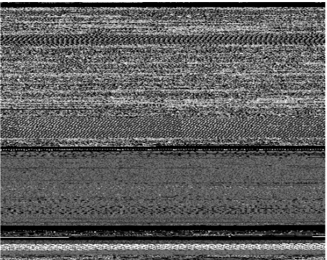
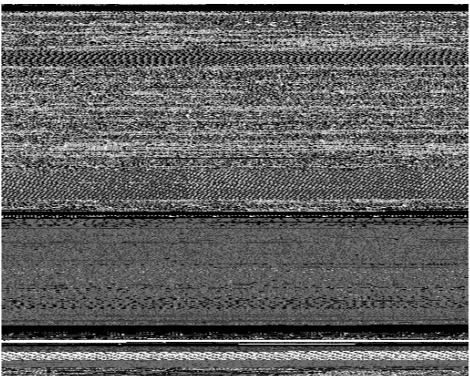
(a) Examples of Adialer.C from MalImg
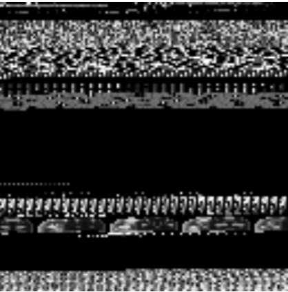
(b) Examples of Obfuscator from MalExe

Figure 1: Images from the MalImg and MalExe datasets

3.2 AC-GAN

A generative adversarial network (GAN) is a type of neural network that—among many other uses—can generate so-called “deep fake” images [37]. A GAN includes a generator model and a discriminative model that compete with each other in a min-max game. Intuitively, this competition will should make both models stronger than if each was trained separately, using only the available training data. The GAN generator generates fake training samples, with the goal of defeating the GAN discriminative model, while the discriminative model tries to distinguish real training samples from fake.

However, a standard GAN is not designed to work with multiclass data. Since we have multiclass data, we use auxiliary-classifier GAN (AC-GAN), which is an enhanced type of GAN that includes a class label in the generative model. Additionally, the discriminator predicts both the class label and the validity (i.e., real or fake) of a given sample. A schematic representation of AC-GAN is given in Figure 2.

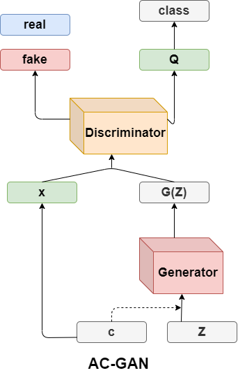
Figure 2: Schematic representation of AC-GAN

For the research in this paper, the key aspect of AC-GAN is that it enables us to have control of the class of any image that we generate. We will also make use of AC-GAN discriminative models, as they will serve as a baseline for comparison to other deep learning techniques—specifically, CNNs and ELMs.

3.3 Evaluation Plan

Once, we have trained and tested our AC-GAN model, we need to evaluate the quality of the fake images. To do this, we compare the AC-GAN classifier to CNN and ELM models trained on real and fake samples. The remainder of this section is devoted to a brief introduction to CNNs and ELMs.

3.3.1 CNN

A convolutional neural network (CNN) is loosely based on the way that a human perceives an image. We first recognize edges, the general shape, texture, and so on, eventually building up to the point where we can identify a complex object.

A CNN is a feed-forward neural network that includes convolution layers in which convolutions (i.e., filters) are applied to produce higher level feature maps. CNNs typically also include pooling layers that primarily serve to reduce the dimensionality of the problem via downsampling. CNNs also typically have a final fully-connected layer, where all inputs from previous layers are mapped to all possible outputs. A generic CNN architecture is given in Figure 3.

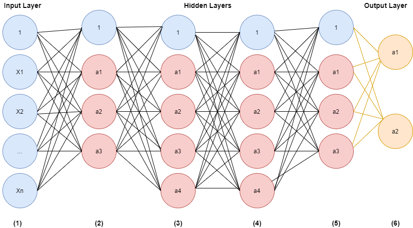
Figure 3: A generic CNN

For our experiments, we will use the specific CNN architecture and hyperparameters specified in [24]. The CNN experiments performed in our research involve malware images, and the specific architecture that we adopt was optimized for precisely this problem.

3.3.2 ELM

A so-called extreme learning machine (ELM) is a feedforward deep learning architecture that does not require any back-propagation. The weights and biases in the hidden layers of an ELM are assigned at random, and only the output weights are determined via training. Due to this simple structure, an ELM can be trained using a straightforward equation solving technique—specifically, the Moore-Penrose generalized inverse. Thus, ELMs are extremely efficient to train. A schematic representation of a generic ELM can be seen in Figure 4.

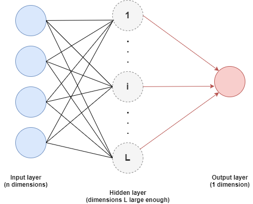
Figure 4: Schematic representation of ELM

For our experiments, we will use ELM models with parameters as specified in [24]. As with the CNN experiments mentioned above, the experiments performed in our research involve malware images, and the specific ELM architecture that we use was optimized for this specific problem.

To evaluate the quality of our AC-GAN generated images, we first divide the real and fake images into training and testing sets. Then we train a CNN (respectively, ELM) on the training dataset. Once, the CNN (respectively, ELM) has been trained, we predict class labels and determine the accuracy of the predictions. The worse the classification accuracy of the CNN (respectively, ELM), the better are our AC-GAN generated fake images. We also want to compare the accuracy of the CNN and ELM models to the AC-GAN discriminator. Note that we consider each real family and each fake family as a separate class, in effect doubling the number of classes from the original dataset.

4 Implementation

In this section, we present details on the implementation of the techniques discussed in Section 3. All of our learning techniques have been implemented in Python using PyTorch and Keras, with the experiments run on Google Colab Pro under a local Windows OS. The precise specifications are given in the Table 3.

Table 3: Environment specifications

Specification Description Local machine Windows OS Intel(R) Core(TM) i7-9750H CPU @ 2.60GHz 16.0 GB RAM NVIDIA GeForce RTX 2060 14GB GPU Google Colab Pro 24 hours available runtime 25 GB memory T4 and P100 GPUs Software PyTorch Keras Numpy Scipy PIL

In the remainder of this section we provide details on the pre-processing applied to the datasets used in our experiments, we outline our AC-GAN training process, and we discuss the training and testing of our CNN and ELM evaluation models. Then in Section 5 we present out experimental results.

4.1 Dataset Analysis and Conversion

As mentioned above, we experiment with two distinct datasets. In both cases, we use the ImageDataGenerator and Dataloader modules from Keras (in PyTorch) to extract images and labels from the data. Additionally we use the transforms functions to compose our pre-processing requirement.

4.1.1 Datasets

The first dataset we consider is the well-known MalImg dataset, which was originally described in [32]. This dataset has become a standard for comparison in image-based malware research. The MalImg dataset contains 9339 grayscale images belonging to 25 classes, where all samples are in the form of images, not executable files.

We refer to our second malware image dataset as MalExe, and it is of our own creation. This dataset contains 24,558 malware images belonging to 18 classes. These samples are in the form of exe files.

Since the MalExe samples are executable binary files, we must converting them to images. We perform this transform as follows. iWe also construct images by specify a desired size of each (square) images as $n\times n$. We then read the first $n^{2}$ bytes from a malware binary, and these bytes are viewed as $n\times n$ images of type png. For example, if we specify $64\times 64$ images, each image is based on the first 4096 bytes of the corresponding exe file. In this conversion process, we only convert samples that contain a sufficient number of bytes. In Table 4, we see the image counts obtained for the MalExe dataset for various image sizes considered. Note that for $512\times 512$ image, we only have 9963 samples from 17 classes—the family Zeroaccess has no samples with at least $512^{2}=2^{18}$ bytes.

Table 4: MalExe dataset counts

Specified image size Count Families Standard 24,652 18 $32\times 32$ 24,557 18 $64\times 64$ 24,371 18 $128\times 128$ 23,369 18 $512\times 512$ 0,9963 17

Figure 5 illustrate images of various sizes for one specific sample from the Alureon family. We see that that these different image construction techniques can provide distinct views of the same data.

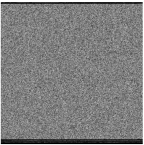
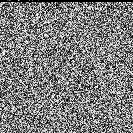
(a) Real	(b) $512\times 512$	(c) $128\times 128$	(d) $64\times 64$	(e) $32\times 32$

Figure 5: Image conversions of an Alureon sample

In Figure 6 we give bar graphs showing the distribution of samples for the MalImg and MalExe datasets. We note that the MalImg dataset is highly imbalanced, with the majority of the images belong to Allaple.A, Allaple.L, and Yuner.A. To deal with this imbalance, we shuffle the data during training and use balanced accuracy while testing.

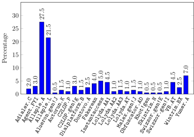
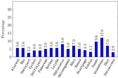
(a) MalImg	(b) MalExe

Figure 6: Distribution of samples among families

Next, we want to scale the pixel values to the range $[-1,1]$ in order to match the output of the generator model. This is achieve by simply calculating the mean pixel value of an entire image and then subtracting this mean from each pixel and normalizing, which gives us a floating point value in the closed interval from $-1$ to $+1$ in place of each pixel value.

4.2 AC-GAN Implementation

In this section, we provide additional detail on our implement of AC-GAN. Recall that our model is generated using Python, PyTorch, and Keras modules. Also, recall that an AC-GAN includes both a generator and a discriminator.

4.2.1 AC-GAN Generator

Our AC-GAN generator produces a single channel grayscale image by plotting random points on a latent space—the latent space simply consists of noise drawn from a Gaussian distribution with $\mu=0$ and $\sigma=1$. Additionally, the model includes the class label as a parameter. The generator is composed as a sequential model. To this sequential model, we add a series of deconvolutional layers. The specific parameters used for the AC-GAN generator are given in the Table 5.

Table 5: AC-GAN generator construction parameters

Layer Functions Parameters Embedding Embedding() $\mbox{classLabels}\times 100$ Sequential() Linear() in-features: 100; out-features: 131, Sequential() $1^{\operatorname{st}}$ convolutional BatchNormal2d() in: 128; momentum: 0.1 Upsample() Scale factor: 2.0 Conv2d() in: 128; out: 128; kernel: (3,3); stride: (1,1); padding: (1,1) $2^{\operatorname{nd}}$ convolutional BatchNormal2d() in: 128; momentum: 0.1 LeakyReLU() negativeslope: 0.2 Upsample() Scale factor: 2.0 Conv2d() in: 128; out: 64; kernel: (3,3); stride: (1,1); padding: (1,1) $3^{\operatorname{rd}}$ convolutional BatchNormal2d() in: 64; momentum: 0.1 LeakyReLU() negativeslope: 0.2 Conv2d() in: 64; outchannels: 1; kernel: (3,3); stride: (1,1); padding: (1,1) Output Tanh() Scale factor: 2.0

4.2.2 AC-GAN Discriminator

The discriminator model discriminates between the original and fake images, while predicting the class label. The generator and discriminator both deal with cross-entropy loss—the generator attempts to minimize binary cross-entropy loss, while the discriminator tries to maximize this loss. The discriminator parameters used in our experiments are given in Table 6.

Table 6: AC-GAN discriminator construction parameters

Layer Functions Parameters Input Sequential() $1^{\operatorname{st}}$ deconvolutional Conv2d() in: 1; out: 16; kernel: (3,3); stride: (2,2); padding: (1,1) $2^{\operatorname{nd}}$ deconvolutional LeakyReLU() negativeslope: 0.2 Dropout2d() rate: 0.25 Conv2d() in: 16; out: 32; kernel: (3,3); stride: (2,2); padding: (1,1) $3^{\operatorname{rd}}$ deconvolutional LeakyReLU() negativeslope: 0.2 Dropout2d() rate: 0.25 BatchNormal2d() in: 32; momentum: 0.1 Conv2d() in: 32; out: 64; kernel: (3,3); stride: (2,2); padding: (1,1) $4^{\operatorname{th}}$ deconvolutional LeakyReLU() negativeslope: 0.2 Dropout2d() rate: 0.25 BatchNormal2d() in: 64; momentum: 0.1 Conv2d() in: 64; out: 128; kernel: (3,3); stride: (2,2); padding: (1,1) LeakyReLU() negativeslope: 0.2 Dropout2d() rate: 0.25 BatchNormal2d() in: 128; momentum: 0.1 Adversarial Sequential() Linear() in-features: 8192; out-features: 1 Sigmoid() Auxiliary Sequential() Linear() in-features: 8192; out-features: 18 Sigmoid()

Once we have initialized the generator and discriminator models, the models are then trained. This training process is typical of any AC-GAN, and hence we omit the details here. After training, we plot loss graphs to verify training stability.

4.3 Evaluation Models

To evaluate our AC-GAN generator results, we train CNN and ELM models on the real and fake images. The better (in some sense) our AC-GAN generated fake images, the worse the CNN and ELM models should perform.

4.3.1 CNN Implementation

CNN models include a fully-connected layer, a convolution layer (or layers), and a pooling layer (or layers). The parameters used in our specific implementation are given in Table 7. The parameters that awe use in our CNN models are as specified in [55]. Note that due to the imbalance in the MalImg dataset, we use balanced accuracy.

Table 7: CNN construction parameters

Layer Functions Parameters $1^{\operatorname{st}}$ convolutional Sequential() Conv2d() filters: 30; $\mbox{in}=\mbox{image-size}$; $\mbox{out}=840$; kernel: (3,3); activation: relu $1^{\operatorname{st}}$ pooling MaxPooling2D() size: (2,2) $2^{\operatorname{nd}}$ convolutional Conv2d() $\mbox{filters}=15$; $\mbox{in}=840$; $\mbox{out}=4065$; kernel: (3,3); activation: relu $2^{\operatorname{nd}}$ pooling MaxPooling2D() size: (2,2) Dropout() rate: 0.25 Flatten() Dense() units: 128; out: 376,448; activation: relu Dropout() rate: 0.5 Other Dense() units: 50; out: 6450; activation: relu Dense() units: num-of-classes; activation: softmax — Loss categorical cross entropy — Optimizer Adam

4.3.2 ELM Implementation

Any ELM includes an initial input layer, a final output layer, and in between these two layers, there is a hidden layer. The hidden layer weights are assigned at random, with only the output layer weights determined via training. For an ELM, the only parameter is the number of hidden units, and we use the value specified in [24], namely 5000.

5 Experimental Results

Here, we first consider the use of AC-GAN to generate fake malware images of various sizes. As part of these experiments, we also consider the discriminative ability of AC-GAN discriminator model.

As a followup on our AC-GAN experiments, we conduct CNN and ELM experiments in Section 5.2. The purpose of these experiments is to determine how well these deep learning techniques can distinguish between real malware images and the AC-GAN generated fake images.

5.1 AC-GAN Experiments

We consider AC-GAN experiments to generate fake malware images of sizes $32\times 32$, $64\times 64$, and $128\times 128$. In each case, we experiment with both the MalImg and MalExe datasets.

5.1.1 AC-GAN with $32\times 32$ Images

Our objective here is generate and classify malware images of size $32\times 32$. For the MalImg dataset, which is in the form of images, we resize all of the images to $32\times 32$. We train our AC-GAN model for 1000 epochs with the number of batches set to 100. Since there are 9400 MalImg samples in total, we have 94 samples per batch, and hence about 94,000 iterations. Training this model requires about 24 hours on Google Colab Pro.

In contrast, for the MalExe dataset we read the first 1024 bytes from each binary, and treat these bytes as a $32\times 32$ image. We train an AC-GAN model on this dataset for 500 epochs with the number of batches set to 50. Since there are 42,266 samples in the MalExe dataset, we have about 492 samples per batch and requires about 246,000 iterations. Training this model also takes about 24 hours on Google Colab Pro.

Figures 7 (a) shows the training loss plots for our AC-GAN generator and discriminator models when training on the MalImg dataset. Figures 7 (b) shows the corresponding loss plots for the MalExe dataset.

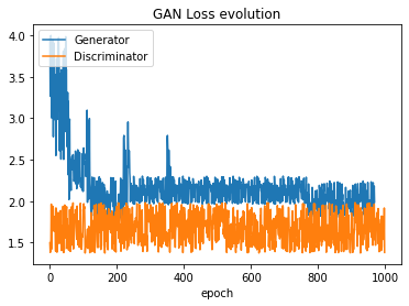
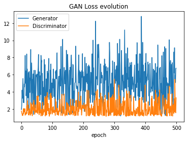
(a) MalImg		(b) MalExe

Figure 7: Loss plot for $32\times 32$ images

From Figure 7 (a), we see that both the generator and discriminator stabilizes at around epoch 100 for the MalImg experiment. The generator spikes up occasionally, but has generally stable loss values, while the discriminator loss is more consistent throughout. In contrast, from Figure 7 (b) we see that the MalExe model remains relatively unstable throughout its 500 iterations.

Our AC-GAN discriminator achieves an accuracy of about 95% in the MalImg experiment. In contrast, on the MalExe dataset, the AC-GAN discriminator only attains an accuracy of about 89%.

Figure 8 shows a comparison of real and AC-GAN generated fake $32\times 32$ images for the families C2LOP.P and Allaple.L from the MalImg dataset. Figure 9 shows a comparison between real and fake images for the Alureon and Zeroaccess families from the MalExe data. Visually the real and fake images share some characteristics, with the MalExe fake images being better than the MalImg case. However, the resolution appears to be too low in all cases. Hence, we perform further AC-GAN experiments based on higher resolution images.

(a) C2LOP.P	(b) C2LOP.P_fake	(c) Allaple.L	(d) Allaple.L_fake

Figure 8: Real and fake examples from MalImg ($32\times 32$)

(a) Alureon	(b) Alureon_fake	(c) Zeroaccess	(d) Zeroaccess_fake

Figure 9: Real and fake examples from MalExe ($32\times 32$)

5.1.2 AC-GAN with $64\times 64$ Images

Our AC-GAN experiments for $64\times 64$ images are analogous to those for $32\times 32$ images, as discussed in Section 5.1.1. Again, the training time for each dataset is about 24 hours. Figures 10 (a) and (b) give the training loss plots for the MalImg and MalExe experiments, respectively.

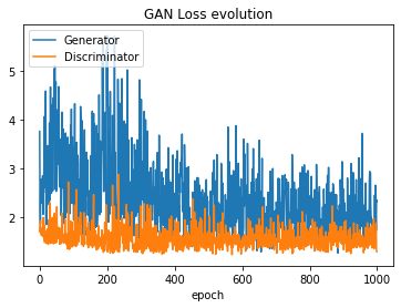
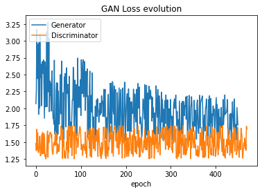
(a) MalImg		(b) MalExe

Figure 10: Loss plot for $64\times 64$ images

From Figure 10 (a), we see that the training loss stabilizes at around epoch 250 for the MalImg case, while the MalExe experiment stabilizes at around epoch 100. In contrast to the $32\times 32$ case, the MalExe model becomes reasonably stable after about 125 epochs.

The classification accuracy for the MalImg dataset is about 94%, while the AC-GAN achieves a classification accuracy of about 88% on the MalExe dataset. These results are essentially the same as in the $32\times 32$ case.

Again, we compare real and AC-GAN generated fake images. Figure 11 shows the comparison between real and fake images of class Lolyda.AA3 and Agent.FYI from the MalImg dataset. We observe that the fake samples in this case are, visually, extremely good.

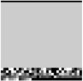
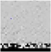
(a) Lolyda.AA3	(b) Lolyda.AA3_fake	(c) Agent.FYI	(d) Agent.FYI_fake

Figure 11: Real and fake examples from MalImg ($64\times 64$)

In Figure 12, we give a comparison between real and fake images of class Zbot and Vobfus for the MalExe dataset. In this case, the MalExe fake samples are surprisingly poor.

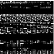
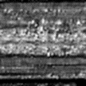
(a) Zbot	(b) Zbot_fake	(c) Vobfus	(d) Vobfus_fake

Figure 12: Real and fake examples from MalExe ($64\times 64$)

5.1.3 AC-GAN with $128\times 128$ Images

We consider AC-GAN experiments based on $128\times 128$ images. These experiments are again analogous to those for the $32\times 32$ and $64\times 64$ cases discussed above. Figures 13 (a) and (b) show the training loss plots for AC-GAN trained on the MalImg and MalExe datasets, respectively. While the MalImg experiments stabilize, the MalExe experiment would likely have benefited from additional iterations.

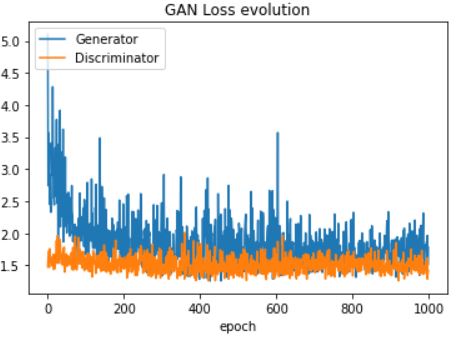
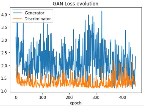
(a) MalImg		(b) MalExe

Figure 13: Loss plot for $128\times 128$ images

In this case, we attain a maximum classification accuracy from the AC-GAN of about 92% for MalImg and about 85% for MalExe. Figure 14 shows comparisons of real and fake Yuner.A and VB.AT from MalImg. As in the $64\times 64$ case, we see that the fake images appear to be very good approximations for this dataset.

(a) Yuner.A	(b) Yuner.A_fake	(c) VB.AT	(d) VB.AT_fake

Figure 14: Real and fake examples from MalImg ($128\times 128$)

Figure 15 shows a comparison of real and fake Alureon and Zeroaccess images from the MalExe data. In contrast to the  $32\times 32$ and $64\times 64$ cases, here the fake MalExe images are very good approximations to the real images.

(a) Alureon	(b) Alureon_fake	(c) Zeroaccess	(d) Zeroaccess_fake

Figure 15: Real and fake examples from MalExe ($128\times 128$)

5.1.4 Summary of AC-GAN Results

Table 8 gives the discriminative accuracies for each of the AC-GAN experiments in Sections 5.1.1 through 5.1.3. We see that the results are fairly consistent, irrespective of the size of the images.

Table 8: AC-GAN discriminator accuracy (rounded to nearest percent)

Image Size Dataset Accuracy $32\times 32$ MalImg 95% MalExe 89% $64\times 64$ MalImg 94% MalExe 88% $128\times 128$ MalImg 92% MalExe 85%

With respect to the visual inspection of the fake images in Figures 8 and 9 (for the $32\times 32$ case), Figures 11 and 12 (for the $64\times 64$ case), and Figures 14 and 15 (for the $128\times 128$ case), we observed a clear improving trend for larger image sizes. However, there is a price to be paid for this increased fidelity, as the training time increases significantly with image size.

5.2 CNN and ELM Experiments

As a first step towards evaluating the quality of the AC-GAN generated images, we experiment with CNN and ELM. Specifically, we test the ability of these two deep learning techniques to distinguish between real malware images and our AC-GAN generated fake images by treating the real data and fake images as distinct classes in multiclass experiments. For example, if we consider 10 classes from the MalImg dataset, then for our CNN and ELM experiments, we will have 20 classes consisting of the 10 original families plus another 10 classes consisting of fake samples from each of the original 10 families. In the following sections, we separately consider experiments for $32\times 32$, $64\times 64$, and $128\times 128$ image sizes.

5.2.1 CNN and ELM for $32\times 32$ Images

Here, we consider $32\times 32$ real and fake images and perform experiments for the MalImg and MalExe datasets. For MalExe, we consider all 18 classes and therefore, including classes for the fake images, we have a total of 36 classes. Our dataset consists of 100 samples for each class, and hence we have 3600 images. We train our CNN for 3000 epochs and we generate an ELM with 5000 hidden units. The CNN test accuracy is only about 51%, in spite of a training accuracy of 100%, which is a sign of overfitting. The ELM performs slightly worse, achieving an accuracy of 48%.

Figures 18 and 19 in the appendix give the confusion matrices for our CNN and ELM experiments on the MalExe dataset. In both cases, we observe that most of the fakes are largely misclassified, but this is not the case for all families. For example, in the CNN experiments, the fake Vundo samples are classified correctly with 100% accuracy, whereas the real Vundo samples are only classified correctly 33% of the time.

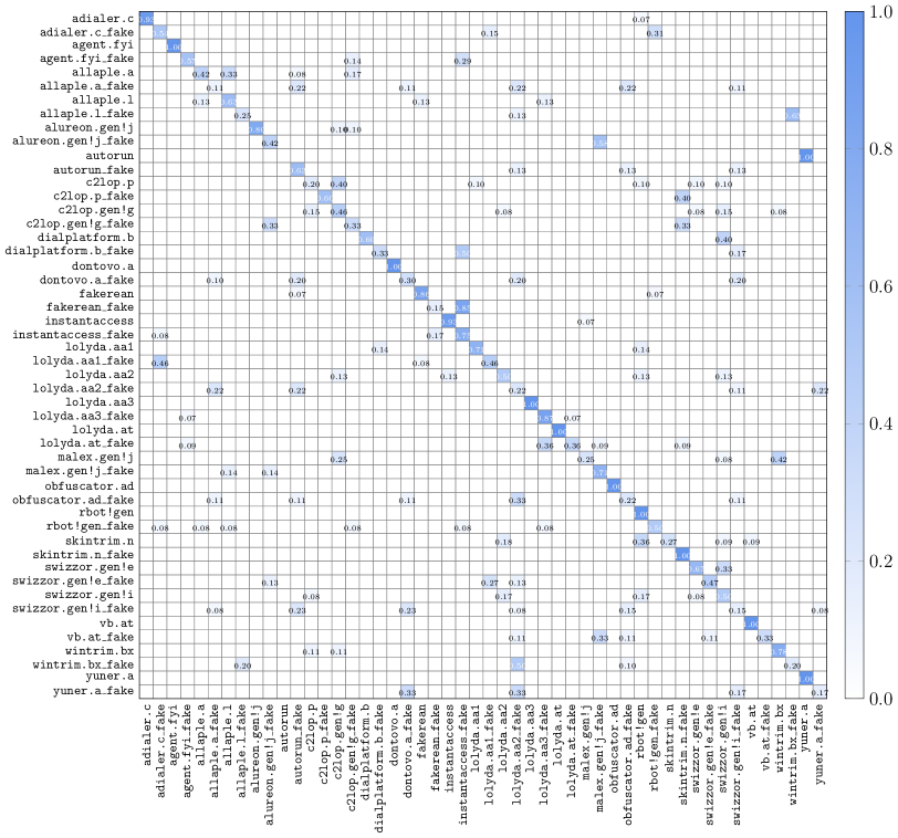
Figure 20: CNN confusion matrix (MalImg $32\times 32$)

For MalImg, we consider all 25 real classes, which gives 50 classes and a total of 5000 images. Again, our CNN is trained for 3000 epochs and we construct an ELM with 5000 hidden units. For the MalImg dataset, our CNN again has a very high training accuracy, but achieves a test accuracy of only about 56%, while our ELM achieves an accuracy of about 37%. The confusion matrices for these experiments are in Figures 20 and 21 in the appendix. Again, we see that the fakes are misclassified at a much higher rate than the real samples.

5.2.2 CNN and ELM for $64\times 64$ Images

In this section, we consider similar experiments as in the previous section, but based on $64\times 64$ images. In this case, we consider 10 of the MalImg families and the corresponding fake samples, for a total of 20 classes for each dataset. We again consider 100 images from each class, and we use 70% of the samples for training and reserve the remaining 30% for testing.

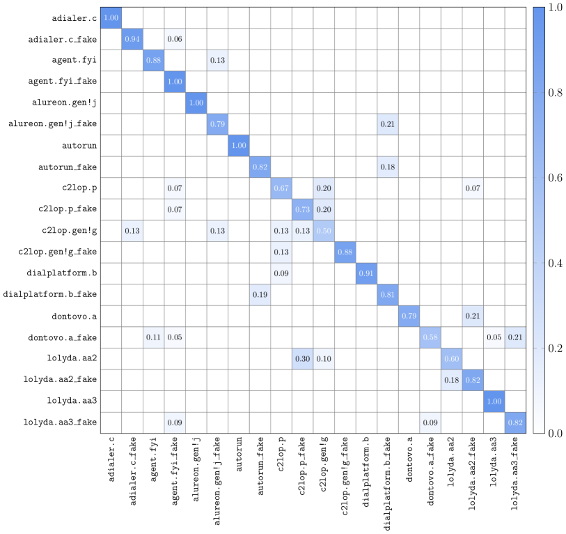
Figure 22: CNN confusion matrix (MalImg $64\times 64$)

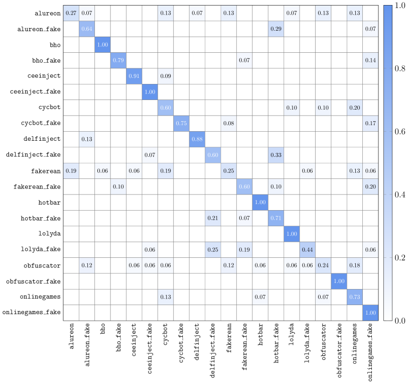
Figure 24: CNN confusion matrix (MalExe $64\times 64$)

We train a CNN for 3000 epochs with a batch size of 500 while for the ELM we use 50,000 hidden units. For the CNN, we attain 100% training accuracy, but only about 82% test accuracy, which is again a sign of overfitting. For the ELM, we attain an accuracy of 64%. Figures 22 and 23 in the appendix show the confusion matrices for these experiments. From the confusion matrices, we can see that some images are misclassified as fakes, while some families are consistently classified as other families. For both the CNN and ELM, we see that most images are misclassified, with the exception of specific families. The $64\times 64$ results—in the form of confusion matrices—for the MalExe dataset are in Figures 24 and 25 in the appendix.

5.2.3 CNN and ELM for $128\times 128$ Images

In this MalImg experiment, we consider all families in the dataset. In this case, we train the CNN for 5000 epochs and generate an ELM with 20,000 hidden units. Again, we treat real and fake images as a separate set of classes. We consider all 18 classes in our MalExe experiments.

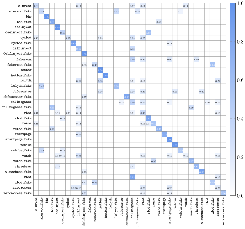
Figure 26: CNN confusion matrix (MalExe $128\times 128$)

On the MalExe dataset, we achieve 43% test accuracy with the CNN, and 52% accuracy with out ELM. Figures 26 and 27 in the appendix show the confusion matrices for our CNN and ELM experiments on the MalExe data. Similar to other experiments on MalExe, we see mostly miscalculation for the CNN. For the ELM, we note that Rbot fake, and Ceeinject fake are particularly poor results. The results of these $128\times 128$ experiments again indicate that AC-GAN produces strong fake images.

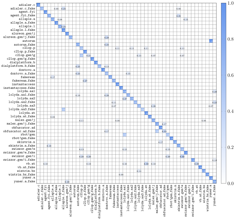
Figure 28: CNN confusion matrix (MalImg $128\times 128$)

For the $128\times 128$ MalImg experiments, we consider all classes, we train the CNN for 3000 epochs, and we generate an ELM with 20,000 hidden units. The results for these MalImg experiments are given in Figures 28 and 29 in the appendix. The CNN achieves only 43% test accuracy, while ELM performs better, but still only attains an accuracy of 52%.

5.2.4 Discussion of CNN and ELM Experiments

In Figure 16 we compare the test accuracies of our CNN and ELM experiments to our AC-GAN classifier. Here, we observe that the AC-GAN models are able to to produce much higher classification rates in all cases. This shows that while the AC-GAN generator is able to produce images that are difficult for other deep learning techniques to distinguish, the AC-GAN discriminator is not so easily defeated by these fake images. These results suggest that AC-GAN is not only a source for generating fake malware images, but it is also a powerful model for discriminating between families—both real and fake.

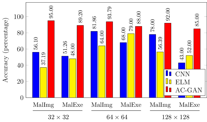
Figure 16: Test accuracy for all experiments

Finally, we consider the narrower problem of distinguishing real samples from fake samples. In Figures 30 through 32 in the appendix, we have “condensed” the confusion matrices of Figures 18 through 29 to better highlight the ability of our CNN and ELM models to distinguish real from fake. Each of these condensed confusion matrices includes the eight (exhaustive) cases listed in Table 9.

Table 9: Condensed confusion matrix cases

Actual class Classification Description real real-same real sample classified correctly fake-same real sample classified as fake of the same family real-other real sample classified as a different real family fake-other real sample classified as a different fake family fake real-same fake sample classified as real of the same family fake-same fake sample classified correctly real-other fake sample classified as a different real family fake-other fake sample classified as a different fake family

If we are only concerned with the ability of our models to distinguish between real and fake samples, then any real sample that is classified as real—either the correct real family or a different real family—is considered a correct classification. Similarly, any fake sample that is classified as any class of fake is considered a correct classification. The results in Figure 17 are easily obtained from the condensed confusion matrices in Figures 30 through 32. From this perspective, we see that our CNN models always outperform the corresponding ELM model, and in most cases, the CNN models perform remarkably well. These results indicate that in spite of the relatively low accuracies obtained in the multiclass case, most of the errors are within the real and fake categories, and not between real and fake samples. In particular, for the CNN models, real and fake samples from a specific family are rarely confused with each other. This provides strong evidence that the real and fake categories are substantially different from each other. Perhaps surprisingly, these results strongly suggest that AC-GAN generated fake malware images do not satisfy the requirements of “deep fakes,” at least not from the perspective of evaluation by deep learning techniques.

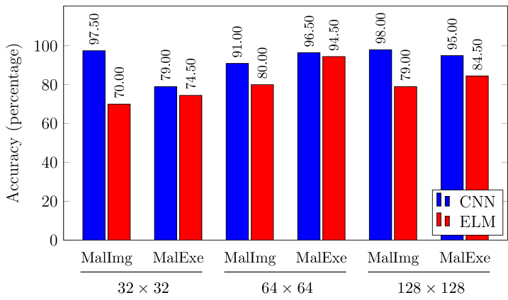
Figure 17: Distinguishing between real and fake

6 Conclusion and Future Work

In this research we considered AC-GAN in the context of malware research. We experimented with a standard malware image dataset (MalImg) and a larger and more balanced malware image dataset of our own construction (MalExe). We evaluated the images generated by our AC-GAN using CNN and ELM models.

We were not able to reliably classify our AC-GAN generated fake malware images from genuine malware images using either CNNs or ELMs, but the AC-GAN discriminator provided good accuracy. However, we also found that CNNs can distinguish between real and AC-GAN generated fake samples with surprisingly high accuracy.

For future work, more experiments aimed at classifying real and fake malware images would be useful. Additional state-of-the-art deep learning models, such as ResNet152 and VGG-19, could be considered [39]. In addition, the quest for true “deep fake” malware images that cannot be reliably distinguished from real malware images appears to be a challenging problem.

In addition, it would be interesting to explore adversarial attacks on image-based malware detectors. For example, tt would be interesting to quantify the effectiveness of such attacks. That is, assuming that an attacker is able to corrupt the training data, what is the minimum percentage of the data that must be modified to achieve a desired level of degradation in the resulting model?

Appendix A Appendix

In this appendix, we give the confusion matrices for each of the $32\times 32$, $64\times 64$, and $128\times 128$ experiments discussed in Sections 5.2.1, 5.2.2 and 5.2.3, respectively.

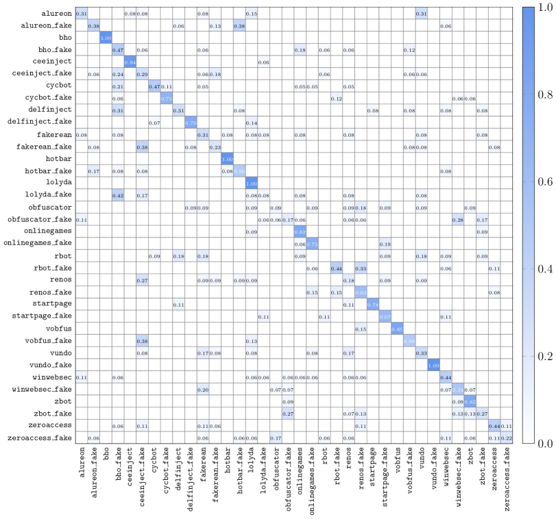
Figure 18: CNN confusion matrix (MalExe $32\times 32$)

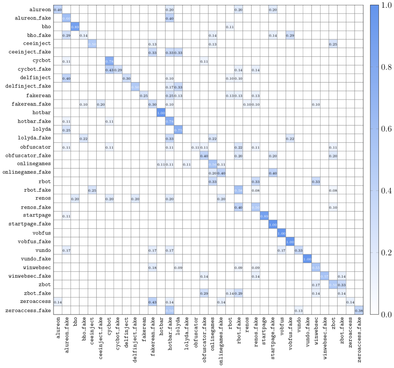
Figure 19: ELM confusion matrix (MalExe $32\times 32$)

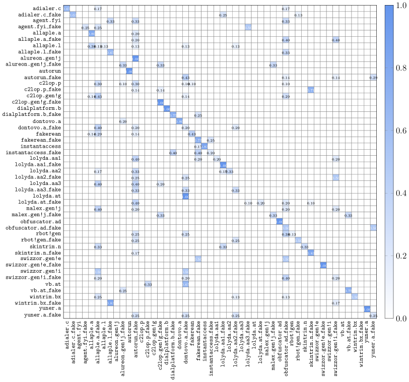
Figure 21: ELM confusion matrix (MalImg $32\times 32$)

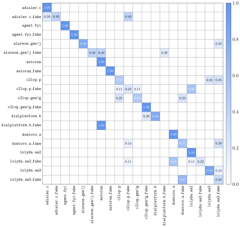
Figure 23: ELM confusion matrix (MalImg $64\times 64$)

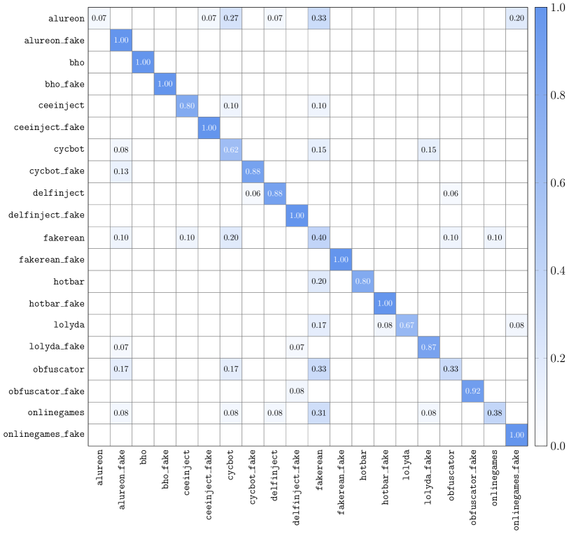
Figure 25: ELM confusion matrix (MalExe $64\times 64$)

Figure 27: ELM confusion matrix (MalExe $128\times 128$)

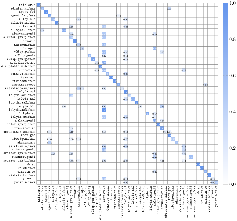
Figure 29: ELM confusion matrix (MalImg $128\times 128$)

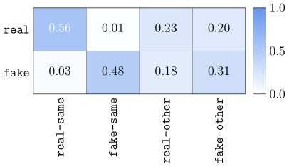
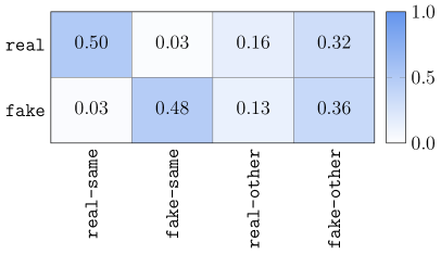
(a) CNN MalExe	(b) ELM MalExe
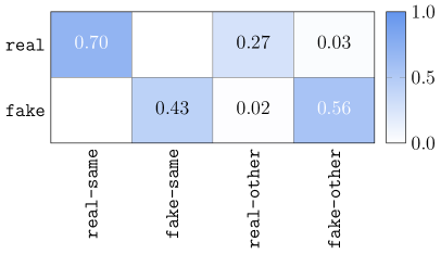
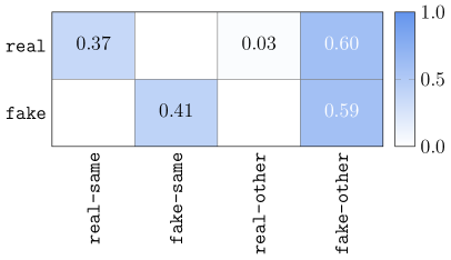
(a) CNN MalImg	(b) ELM MalImg

Figure 30: Condensed confusion matrices ($32\times 32$)

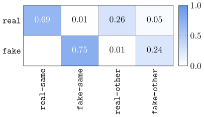
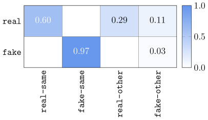
(a) CNN MalExe	(b) ELM MalExe
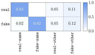
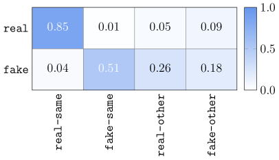
(a) CNN MalImg	(b) ELM MalImg

Figure 31: Condensed confusion matrices ($64\times 64$)

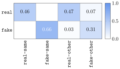
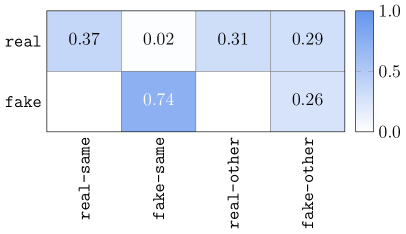
(a) CNN MalExe	(b) ELM MalExe
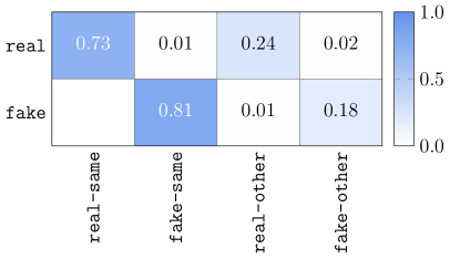
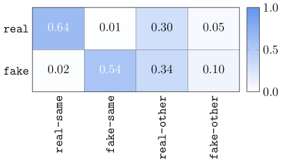
(a) CNN MalImg	(b) ELM MalImg

Figure 32: Condensed confusion matrices ($128\times 128$)

References

- [1] Adialer.c. https://www.microsoft.com/en-us/wdsi/threats/malware-encyclopedia-description?Name=Trojan:Win32/Adialer.C&threatId=-2147460766.
- [2] Agent.fyi. https://www.microsoft.com/en-us/wdsi/threats/malware-encyclopedia-description?Name=Exploit:Win32/Siveras.A.
- [3] Allaple.a. https://www.microsoft.com/en-us/wdsi/threats/malware-encyclopedia-description?Name=worm:win32/allaple.a&ThreatID=2147574777.
- [4] Allaple.l. https://www.microsoft.com/en-us/wdsi/threats/malware-encyclopedia-description?Name=Worm:Win32/Allaple.L.
- [5] Alureon. https://www.microsoft.com/en-us/wdsi/threats/malware-encyclopedia-description?Name=Win32/Alureon.
- [6] Alureon.gen!j. https://www.microsoft.com/en-us/wdsi/threats/malware-encyclopedia-description?Name=Trojan:Win32/Alureon.gen!J.
- [7] Autorun.k. https://www.microsoft.com/en-us/wdsi/threats/malware-encyclopedia-description?Name=Worm:Win32/Autorun.K&threatId=-2147369124.
- [8] Bho. https://www.microsoft.com/en-us/wdsi/threats/malware-encyclopedia-description?Name=Trojan:Win32/BHO&threatId=-2147364778.
- [9] C2lop.gen!g. https://www.microsoft.com/en-us/wdsi/threats/malware-encyclopedia-description?Name=Trojan:Win32/C2Lop.gen!G&threatId=139219.
- [10] C2lop.p. https://www.microsoft.com/en-us/wdsi/threats/malware-encyclopedia-description?Name=Trojan:Win32/C2Lop.P.
- [11] Bugra Cakir and Erdogan Dogdu. Malware classification using deep learning methods. In Proceedings of the ACMSE 2018 Conference, pages 1–5, 2018.
- [12] Ceeinject. https://www.microsoft.com/en-us/wdsi/threats/malware-encyclopedia-description?Name=VirTool%3AWin32%2FCeeInject.
- [13] Gregory Conti, Sergey Bratus, Anna Shubina, Andrew Lichtenberg, Roy Ragsdale, Robert Perez-Alemany, Benjamin Sangster, and Matthew Supan. A visual study of primitive binary fragment types. https://www.semanticscholar.org/paper/A-Visual-Study-of-Primitive-Binary-Fragment-Types-Conti-Bratus/b406e34d0c203deadfb028f14607bfe88e5763ac, 2010.
- [14] Cycbot. https://www.microsoft.com/en-us/wdsi/threats/malware-encyclopedia-description?Name=Win32/Cycbot&threatId=.
- [15] Dennis Dang, Fabio Di Troia, and Mark Stamp. Malware classification using long short-term memory models. https://arxiv.org/abs/2103.02746, 2021.
- [16] Delfinject. https://www.microsoft.com/en-us/wdsi/threats/malware-encyclopedia-description?Name=PWS:Win32/DelfInject&threatId=-2147241365.
- [17] Diaplatform.b. https://www.microsoft.com/en-us/wdsi/threats/malware-encyclopedia-description?Name=Dialer:Win32/DialPlatform.B.
- [18] Dontovo.a. https://www.microsoft.com/en-us/wdsi/threats/malware-encyclopedia-description?Name=TrojanDownloader:Win32/Dontovo.A&threatId=-2147342037.
- [19] Fakerean. https://www.microsoft.com/en-us/wdsi/threats/malware-encyclopedia-description?Name=Win32/FakeRean.
- [20] Hotbar. https://www.microsoft.com/en-us/wdsi/threats/malware-encyclopedia-description?Name=Adware:Win32/Hotbar&threatId=6204.
- [21] Weiwei Hu and Ying Tan. Generating adversarial malware examples for black-box attacks based on GAN. https://arxiv.org/abs/1702.05983, 2017.
- [22] Nathan Inkawhich. PyTorch DCGAN tutorial. https://pytorch.org/tutorials/beginner/dcgan_faces_tutorial.html.
- [23] Instantaccess. https://www.microsoft.com/en-us/wdsi/threats/malware-encyclopedia-description?name=dialer:win32/instantaccess.
- [24] Mugdha Jain. Image-based malware classification with convolutional neural networks and extreme learning machines. https://scholarworks.sjsu.edu/etd_projects/900/, 2019.
- [25] Masataka Kawai, Kaoru Ota, and Mianxing Dong. Improved MalGAN: Avoiding malware detector by leaning cleanware features. In 2019 International Conference on Artificial Intelligence in Information and Communication, ICAIIC, pages 040–045, 2019.
- [26] Jin-Young Kim, Seok-Jun Bu, and Sung-Bae Cho. Malware detection using deep transferred generative adversarial networks. In International Conference on Neural Information Processing, pages 556–564, 2017.
- [27] David Kornish, Justin Geary, Victor Sansing, Soundararajan Ezekiel, Larry Pearlstein, and Laurent Njilla. Malware classification using deep convolutional neural networks. In 2018 IEEE Applied Imagery Pattern Recognition Workshop, AIPR, pages 1–6, 2018.
- [28] Lolyda. https://www.microsoft.com/en-us/wdsi/threats/malware-encyclopedia-description?Name=PWS%3AWin32%2FLolyda.BF.
- [29] Lolyda.aa1. https://www.microsoft.com/en-us/wdsi/threats/malware-encyclopedia-description?Name=PWS:Win32/Lolyda.AA&threatId=-2147345828.
- [30] Lolyda.at. https://www.microsoft.com/en-us/wdsi/threats/malware-encyclopedia-description?Name=PWS:Win32/Lolyda.AT&ThreatID=2147627867.
- [31] Yan Lu and Jiang Li. Generative adversarial network for improving deep learning based malware classification. In 2019 Winter Simulation Conference, WSC, pages 584–593, 2019.
- [32] Adam Lutz, Victor F. Sansing III, Waleed E. Farag, and Soundararajan Ezekiel. Malware classification using fusion of neural networks. In Misty Blowers, Russell D. Hall, and Venkateswara R. Dasari, editors, Disruptive Technologies in Information Sciences II, pages 165–170. SPIE, 2019.
- [33] Malex.gen!j. https://www.microsoft.com/en-us/wdsi/threats/malware-encyclopedia-description?Name=Trojan:Win32/Malex.gen!J.
- [34] McAfee 2020 2nd quarter report. https://www.mcafee.com/enterprise/en-us/lp/threats-reports/apr-2021.html.
- [35] Lakshmanan Nataraj, Sreejith Karthikeyan, Gregoire Jacob, and Bangalore S Manjunath. Malware images: Visualization and automatic classification. In Proceedings of the 8th International Symposium on Visualization for Cyber Security, pages 1–7, 2011.
- [36] Obfuscator. https://www.microsoft.com/en-us/wdsi/threats/malware-encyclopedia-description?Name=Win32/Obfuscator&threatId=.
- [37] Augustus Odena, Christopher Olah, and Jonathon Shlens. Conditional image synthesis with auxiliary classifier GANs. https://arxiv.org/abs/1610.09585, 2017.
- [38] Onlinegames. https://www.microsoft.com/en-us/wdsi/threats/malware-encyclopedia-description?Name=PWS%3AWin32%2FOnLineGames, journal=Onlinegames.
- [39] Pratikkumar Prajapati and Mark Stamp. An empirical analysis of image-based learning techniques for malware classification. In Malware Analysis Using Artificial Intelligence and Deep Learning, pages 411–435. Springer, 2020.
- [40] Rbot. https://www.microsoft.com/en-us/wdsi/threats/malware-encyclopedia-description?Name=Win32/Rbot&threatId=.
- [41] Rbot!gen. https://www.microsoft.com/en-us/wdsi/threats/malware-encyclopedia-description?Name=Backdoor:Win32/Rbot.gen.
- [42] Renos. https://www.microsoft.com/en-us/wdsi/threats/malware-encyclopedia-description?Name=TrojanDownloader:Win32/Renos&threatId=16054.
- [43] Igor Santos, Javier Nieves, and Pablo G Bringas. Semi-supervised learning for unknown malware detection. In International Symposium on Distributed Computing and Artificial Intelligence, pages 415–422, 2011.
- [44] Skintrim.n. https://www.microsoft.com/en-us/wdsi/threats/malware-encyclopedia-description?Name=Trojan:Win32/Skintrim.N.
- [45] Startpage. https://www.microsoft.com/en-us/wdsi/threats/malware-encyclopedia-description?Name=Trojan:Win32/Startpage&threatId=15435.
- [46] Guosong Sun and Quan Qian. Deep learning and visualization for identifying malware families. IEEE Transactions on Dependable and Secure Computing, 18(1):283–295, 2021.
- [47] Swizzor.gen!e. https://www.microsoft.com/en-us/wdsi/threats/malware-encyclopedia-description?Name=TrojanDownloader%253aWin32%252fSwizzor.gen!E&navV3Index=3, key=Swizzor.gen!E.
- [48] Swizzor.gen!i. https://www.microsoft.com/en-us/wdsi/threats/malware-encyclopedia-description?Name=TrojanDownloader:Win32/Swizzor.gen!I.
- [49] Vb.at. https://www.microsoft.com/en-us/wdsi/threats/malware-encyclopedia-description?Name=Worm:Win32/VB.AT.
- [50] Vobfus. https://www.microsoft.com/en-us/wdsi/threats/malware-encyclopedia-description?Name=Win32/Vobfus&threatId=.
- [51] Vundo. https://www.microsoft.com/en-us/wdsi/threats/malware-encyclopedia-description?Name=Win32/Vundo&threatId=.
- [52] Wintrim.bx. https://www.microsoft.com/en-us/wdsi/threats/malware-encyclopedia-description?Name=TrojanDownloader:Win32/Wintrim.BX.
- [53] Winwebsec. https://www.microsoft.com/en-us/wdsi/threats/malware-encyclopedia-description?Name=Win32/Winwebsec.
- [54] Sravani Yajamanam, Vikash Raja Samuel Selvin, Fabio Di Troia, and Mark Stamp. Deep learning versus gist descriptors for image-based malware classification. In Paolo Mori, Steven Furnell, and Olivier Camp, editors, Proceedings of the 4th International Conference on Information Systems Security and Privacy, ICISSP 2018, pages 553–561, 2018.
- [55] Songqing Yue. Imbalanced malware images classification: A CNN based approach. https://arxiv.org/abs/1708.08042, 2017.
- [56] Yuner.a. https://www.microsoft.com/en-us/wdsi/threats/malware-encyclopedia-description?Name=Worm:Win32/Yuner.A&ThreatID=2147600986.
- [57] Zbot. https://www.microsoft.com/en-us/wdsi/threats/malware-encyclopedia-description?Name=PWS:Win32/Zbot&threatId=-2147368817.
- [58] Zeroaccess. https://www.symantec.com/security-center/writeup/2011-071314-0410-99.