Estimating Counts Through an Average Rounded to the Nearest Non-negative Integer and its Theoretical & Practical Effects

Abstract

In practice, the use of rounding is ubiquitous. Although researchers have looked at the implications of rounding continuous random variables, rounding may be applied to functions of discrete random variables as well. For example, to infer on suicide excess deaths after a national emergency, authorities may provide a rounded average of deaths before and after the emergency started. Suicide rates tend to be relatively low around the world and such rounding may seriously affect inference on the change of suicide rate. In this paper, we study the scenario when a rounded to nearest integer average is used as a proxy for a non-negative discrete random variable. Specifically, our interest is in drawing inference on a parameter from the pmf of $Y$, when we get $U=n[Y/n]$ as a proxy for $Y$. The probability generating function of $U$, $\operatorname{E}(U)$, and $\operatorname{Var}(U)$ capture the effect of the coarsening of the support of $Y$. Also, moments and estimators of distribution parameters are explored for some special cases. We show that under certain conditions, there is little impact from rounding. However, we also find scenarios where rounding can significantly affect statistical inference as demonstrated in three examples. The simple methods we propose are able to partially counter rounding error effects. While for some probability distributions it may be difficult to derive maximum likelihood estimators as a function of $U$, we provide a framework to obtain an estimator numerically.

1 Introduction

The need to study the effects of rounding is appreciated more naturally in the realm of continuous random variables. For example, children occipito-frontal circumference measures, which are important markers of cerebral development, are customarily recorded to the nearest centimeter and such rounding could mask contrasts (Wang and Wertelecki, 2013). Weight may be rounded to the nearest pound, and age rounded to the nearest year. The effects of rounding on the first two moments of the probability distribution of a continuous random variable were considered by Tricker (1984), while Tricker (1990); Tricker et al (1998) considered the effects of rounding errors on Type I errors, power and R charts. The characteristic function, moments and oscillatory behavior of rounded continuous random variables were investigated by Janson (2006); Pace et al (2004) studied the properties of likelihood procedures after decimal point rounding, Wang and Wertelecki (2013) suggested rounding errors may affect statistical inference, and Chen (2021) defined non-asymptotic moment bounds for rounded random variables. Many of these studies have found that rounded random variables can have similar properties to the true (hidden) random variable counterparts. Yet it is unclear how generally good the approximation is. Moreover, the exponential growth in data (Beath et al, 2012; Rivera et al, 2019; Rivera, 2020), recent tendencies in deep learning to lower precision (Rodriguez et al, 2018; Wang et al, 2018; Colangelo et al, 2018; Gupta et al, 2015), and development of physically informed machine learning models (Raissi et al, 2017; Rao et al, 2020; Hooten et al, 2011; Wikle and Hooten, 2010) make it paramount to better understand the effects of rounding and truncation error (Kutz, 2013).

Our emphasis is on the effects of rounding for a non-negative discrete count random variable. Say $Y=X_{1}+...+X_{n}$ are the total counts from $n$ independent measurements and the random variable has some probability mass function (pmf), $P_{Y}(y)$, parameterized by $\nu$. However, instead of obtaining $Y$ directly, only an average over the $n$ measurements rounded to the nearest non-negative integer is available which is then used to estimate the counts. Define $[X]$ as $X$ rounded to the nearest integer. The rounded average random variable is $[\frac{Y}{n}]$ and an estimator of the count may be expressed as

$$U=n[\frac{Y}{n}]$$

where $n\geq 1$. Whether $u$ has an upper bound or not depends on the pmf of $Y$. $[\frac{Y}{n}]$ has support $0,1,..$ so $u\in\{0,n,2n,...\}$; a multiplier of $n$. When $n=1$, then $Y=u$. Since $n$ is fixed, it is possible that $P(U=y)=0$ for some $y$ although $P(Y=y)\neq 0$. For example, if $n=3$, then $P(n[\frac{Y}{n}]=10)=0$ even if $P(Y=10)\neq 0$. From the support of $U$ it is clear that a noticeable binning of $Y$ values occurs and the larger the $n$, the more separated the support values of $U$ become. This is a form of coarsening (Taraldsen, 2011). Because the average is rounded to the nearest integer, attempting to estimate the total by $U$ and treating it as $Y$ will not adequately account for uncertainty. Our aim is to study how using $U$ as a proxy for $Y$ affects inference on $\nu$.

Consider comparing counts between two different periods of time. Instead of having access to true counts, $X_{1}$ for period 1, and $X_{2}$ for period 2, we instead are provided with $[\frac{X_{1}}{n_{1}}]$ and $[\frac{X_{2}}{n_{2}}]$ which we then use to get $U_{1}$ for period 1, $U_{2}$ for period 2; values that we rely on to infer on the difference in true mean counts of both periods. Take how mortality patterns may change during an emergency. Mortality is often underestimated for pandemics, heatwaves, influenza, natural disasters, and other emergencies, times when accurate mortality estimates are crucial for emergency response (Rivera et al, 2020; Lugo and Rivera, 2023). The Covid-19 pandemic has made it more apparent than ever that determining the death toll of serious emergencies is difficult (Rosenbaum et al, 2021). Excess mortality estimates can yield a complementary assessment of mortality. Excess mortality can be estimated using statistical models to evaluate whether the number of deaths during an emergency is greater than would be expected from past mortality patterns by comparing the total deaths for period 1 with total deaths for period 2. If excess mortality estimates exceed the official death count from the emergency, the official death count may be an under-estimate. Excess death models have shown discrepancies with the official death toll from the Covid-19 pandemic (Rivera et al, 2020), Hurricane Katrina (Kutner et al, 2009; Stephens et al, 2007), Hurricane Maria (Rivera and Rolke, 2018, 2019; Santos-Lozada and Howard, 2018; Santos-Burgoa et al, 2018; Kishore et al, 2018), heatwaves (Canoui-Poitrine et al, 2006; Tong et al, 2010) and other emergencies. How would statistical inference be affected when using $U_{1}$ and $U_{2}$ as proxies for $X$ and $Y$ respectively when drawing inference on expected difference on mean mortality?

This article is structured as follows. Section 2 presents some theoretical properties of $U$. The special cases when $Y$ follows a Poisson distribution and when it follows a binomial distribution are also studied. Section 3 demonstrates the developed theory through three examples: estimating excess deaths, estimating probability of success, and assessing the effect of rounding through numerical likelihood maximization. We summarize our findings and their implications in Section 4. Proofs of all theorems and corollaries are relayed to the Appendix.

2 Properties of the Proxy Random Variable $U$

Scientists often round data and then misspecify the probability distribution of the proxy random variable. For example, Tilley et al (2019) round raw catch per unit effort fishing data and then models this data as a Poisson random variable. In our context, the proxy random variable $U$ may have a probability distribution that is significantly different than $Y$.

Lemma 1.

If $\lfloor x\rfloor$ maps $x$ to the greatest integer less than or equal to $x$, $\lceil x\rceil$ maps $x$ to the least integer greater than or equal to $x$, $Y$ is a non-negative discrete random variable, and $U=n[\frac{Y}{n}]$, then,

$$P(U=u) = \sum_{q=0}^{n-1-g(u)}P\Bigl{(}Y=h(u)+q+g(u)\Bigr{)}\hskip 14.22636ptu\in\{0,n,2n,..\}$$ (1)

where,

$$g(u) = \begin{cases}\lfloor\frac{n}{2}\rfloor\hskip 14.22636ptu=0\\ 0\hskip 14.22636ptu\geq 1\end{cases}$$ (2)

and

$$h(u) = \begin{cases}u-\frac{n}{2}+\frac{1}{2}\hskip 14.22636ptn\text{ is odd}\\ u-\frac{n}{2}\hskip 14.22636ptn\text{ is even}\end{cases}$$

More succinctly, $h(u)=\lceil u-\frac{n}{2}\rceil$.

Note that when $n=1$, then $P(U=u)=P(Y=u)$. Lemma 1 assumes round half up tie breaking rule is used. If $n$ is even, the pmf will depend on the type of of tie breaking rule used (a tie is when the fraction of the average is 0.5). If the round half to even rule is used, then it can be shown that (see the Appendix),

$$P(U=u) = \begin{cases}\sum_{q=0}^{n}P(Y=u-\frac{n}{2}+q)&u/n\text{ is even}\\ \sum_{q=0}^{n-2}P(Y=u-\frac{n}{2}+1+q)&u/n\text{ is odd}\\ \end{cases}$$

The rest of this paper proceeds according to the round half up tie breaking rule. This was a pragmatic choice, as the rule made theoretical results more compact and did not have an effect on the overall conclusions of the paper.

Turning to moments, the expected value of $U$ is

$$\operatorname{E}(U)=\sum_{u_{k}\in\mathcal{U}}u_{k}P(U=u_{k})$$

where $\mathcal{U}$ is the support of $U$. Observe from (1) that the pmf of $U$ for the most part aggregates the probabilities of $n$ values of $Y.$ Thus, to calculate moments of $U$ as a function of $Y,$ a projection is useful so that moments of $U$ are a function of moments of $Y$. To accomplish this, first we derive an expression for the probability generating function (Resnick, 1992), pgf, of $U$ from the pgf of $Y,$

$$G_{Y}(s)=\operatorname{E}(s^{Y})=\sum_{y=0}^{\infty}p_{y}s^{y}=p_{0}+p_{1}s+p_{2}s^{2}+\cdots p_{n}s^{n}+\cdots$$

where $p_{y}=P(Y=y)$ and the sum converges for any $s\in{\rm I\!R}$ such that $\mid s\mid\leq 1$.

Theorem 1.

If $Y$ is a non-negative discrete random variable, let $U=n[\frac{Y}{n}]$, and $\omega=exp(\frac{2\pi i}{n})$. Then the pgf of $U$ is,

$$G_{U}(s) = \frac{(s^{n}-1)}{ns^{n/2-r}}\sum_{j=0}^{n-1}a(j)\frac{G_{Y}(s/\omega^{j})}{s-\omega^{j}}$$ (3)

where

$$r = \begin{cases}1\hskip 14.22636ptn\text{ is even}\\ 1/2\hskip 14.22636ptn\text{ is odd}\end{cases}$$

and

$$a(j) = \begin{cases}(-1)^{j}\hskip 14.22636ptn\text{ is even}\\ (-1)^{j}\omega^{j/2}\hskip 14.22636ptn\text{ is odd}\end{cases}$$

Thus, when $n=1$ $G_{U}(s)=G_{Y}(s)$, and when $n=2$,

$$G_{U}(s) = \frac{1}{2}\Bigl{(}(s+1)G_{Y}(s)-(s-1)G_{Y}(-s)\Bigr{)}$$

Notice from (3) that $\omega$ combined with $a(j)$ will lead to non-negligible oscillatory behavior of the moments of $U$ as we will see later on. For large $n$, if $p_{y}\rightarrow 0$ as $y$ increases then less terms in the summation in (3) will be different from zero, giving $G_{U}(s)$ a simpler form. Theorem 1 helps us find expressions for moments of $U$ as a function of moments of $Y$ and therefore better understand the impact of rounding.

Theorem 2.

For any non-negative discrete random variable $Y,$ if $U=n[\frac{Y}{n}]$ and $\omega=exp(\frac{2\pi i}{n})$, then:

$$\operatorname{E}(U) = \operatorname{E}(Y)+\frac{1}{2}\left(2r-1\right)+\sum^{n-1}_{j=1}a(j)\frac{G_{Y}(\frac{1}{\omega^{j}})}{1-\omega^{j}}$$ (4)

and

$$\operatorname{Var}(U) = \operatorname{Var}(Y)+\frac{1}{12}(n^{2}-1)-\left(2\operatorname{E}(Y)-1\right)\sum^{n-1}_{j=1}a(j)\frac{G_{Y}(\frac{1}{\omega^{j}})}{1-\omega^{j}}$$ (5)

$$-\left(\sum^{n-1}_{j=1}a(j)\frac{G_{Y}(\frac{1}{\omega^{j}})}{1-\omega^{j}}\right)^{2}$$

$$+2\sum^{n-1}_{j=1}a(j)\left(\frac{G_{Y}^{{}^{\prime}}(\frac{1}{\omega^{j}})}{\omega^{j}(1-\omega^{j})}-\frac{G_{Y}(\frac{1}{\omega^{j}})}{\left(1-\omega^{j}\right)^{2}}\right)$$

where

$$r = \begin{cases}1\hskip 14.22636ptn\text{ is even}\\ 1/2\hskip 14.22636ptn\text{ is odd}\end{cases}$$

and

$$a(j) = \begin{cases}(-1)^{j}\hskip 14.22636ptn\text{ is even}\\ (-1)^{j}\omega^{j/2}\hskip 14.22636ptn\text{ is odd}\end{cases}$$

Let’s take a moment to take in the results up until now and examine properties of $U$ as $n\to\infty$. According to Lemma 1, $P(U=u)\approx P(u-\frac{n}{2}\leq Y\leq u-\frac{n}{2})$. As $n\to\infty$ the support of $U$ becomes more spread out, and probability mass of $U$ must concentrate on less values of the random variable. Figure 1 illustrates how $U$ coarsens the support of $Y\sim Poisson(\theta=2)$; the higher the sample size, the more drastic the coarsening. At $n=10$, treating $U$ as a Poisson random variable would lead us to underestimate $\theta$.

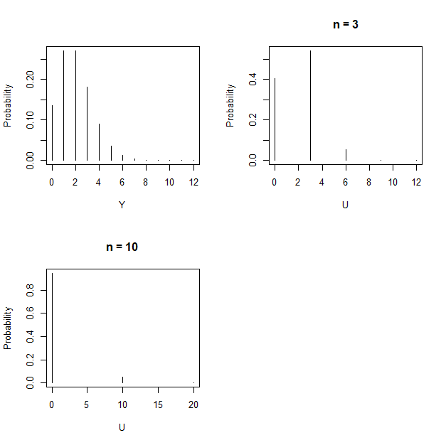
Figure 1: Upper left panel shows the pmf of $Y\sim Poisson(\theta=2)$. Upper right panel presents the pmf of $U$ when $n=3$ while lower left panel shows the pmf of $U$ when $n=10$.

Equation (5) is similar to the proposed Sheppard’s correction Sheppard (1898); Tricker et al (1998); Schneeweiß et al (2010) except that Sheppard’s correction ignores that the rounded random variable $U$ and the rounded error are dependent on $Y$ Zhao and Bai (2020). Furthermore, (4) and (5) include alternating series terms dependent on $\omega$, and for large $n$ the difference between successive terms in each series is small.

However, the summation terms in (4) and (5) will also depend on distribution parameters values relative to $n$. To look further into this, let $X_{k}$ be independent and identically distributed (iid) non-negative discrete random variables with finite mean $\lambda$ and finite variance $\sigma^{2}$. Define $Y=\sum_{k=1}^{n}X_{k}$. By the central limit theorem, $Y/n$ will get close to $\lambda$ with smaller variance as $n\to\infty$. When $\lambda\in\mathbb{Z}^{+}$, then rounding will not have much effect; $\operatorname{E}(U)\to n\lambda$ and $\operatorname{Var}(U)\to 0$. For non-integer $\lambda$, the parameter has a nonzero fractional part and therefore the rounding will play a role. When $n$ is much larger than $\lambda$, fractional parts less than 0.5 will result in $\operatorname{E}(U)\to n[\lambda]<<n\lambda$, and fractional parts greater than 0.5 will result in $\operatorname{E}(U)\to n[\lambda]>>n\lambda$. Despite this behavior of $\operatorname{E}(U)$, for non-integer $\lambda$ we still have $\operatorname{Var}(U)\to 0$. As the fractional part tends to 0.5, $\operatorname{Var}(U)$ becomes larger than $\operatorname{Var}(Y)$, with their separation increasing as $n$ becomes large.

2.1 Poisson Distribution Case

Now we explore working with $U$ when $Y\sim Poisson(\theta)$. From (1) we have

$$P(U=u) = \sum_{q=0}^{n-1-g(u)}\frac{\theta^{h(u)+q+g(u)}e^{-\theta}}{(h(u)+q+g(u))!}\hskip 14.22636ptu\in\{0,n,2n,..\}$$

$$= \begin{cases}\theta^{h(u)+g(u)}e^{-\theta}\sum_{q=0}^{n-1-g(u)}\frac{\theta^{q}}{(h(u)+q+g(u))!}\hskip 14.22636ptn\geq 2\\ \frac{\theta^{u}e^{-\theta}}{u!}\hskip 14.22636ptn=1\end{cases}$$

As expected, for $n=1$, $P(U=u)$ is the Poisson pmf.

Our intention is to draw inference on $\theta$ using $U$ instead of $Y$. Specifically, we study whether the rounding leads to substantial differences between $\operatorname{E}(U),\operatorname{Var}(U)$ and $\theta$. If we consider that $Y$ is counting events over $n$ periods such that each has independent counts $X_{k}\sim Poisson(\lambda_{k})$, then $Y=\sum_{k=1}^{n}X_{k}\sim Poisson(\sum_{k=1}^{n}\lambda_{k})$ and $\operatorname{E}(U)$ would also be increasing with $n$ since $\theta=\sum_{k=1}^{n}\lambda_{k}$. Assuming all $X_{k}$ are identically distributed, as $n\rightarrow\infty$ $\sum_{k=1}^{n}X_{k}/n\rightarrow\lambda$. However, if $\lambda=0.4$ and $n\rightarrow 10000$, then $\sum_{k=1}^{n}X_{k}/n\rightarrow 0.4$ means that $U\rightarrow 0$, although $\theta=4000$. In contrast, if $\lambda=0.6$ and $n\rightarrow 10000$, then $\sum_{k=1}^{n}X_{k}/n\rightarrow 0.6$ means that $U\rightarrow 10000$, although $\theta=6000$. That is, we can’t generally say that for any $\lambda$, $\operatorname{bias}(U)\rightarrow 0$ as $n\rightarrow\infty$ (the bias of $U$ as an estimator of $n\lambda$).

Corollary 1.

If $Y\sim Poisson(\theta)$, $U=n[\frac{Y}{n}]$ and $\omega=exp(\frac{2\pi i}{n})$, then

$$\operatorname{E}(U) = \theta+\frac{1}{2}(2r-1)+e^{-\theta}\sum^{n-1}_{j=1}a(j)\frac{e^{\frac{\theta}{\omega^{j}}}}{1-\omega^{j}}$$ (7)

and

$$\operatorname{Var}(U) = \theta+\frac{1}{12}(n^{2}-1)-e^{-2\theta}\left(\sum^{n-1}_{j=1}a(j)\frac{e^{\frac{\theta}{\omega^{j}}}}{1-\omega^{j}}\right)^{2}$$ (8)

$$-\sum^{n-1}_{j=1}a(j)\frac{e^{\frac{\theta}{\omega^{j}}}}{1-\omega^{j}}\left(\frac{2e^{-\theta}}{1-\omega^{j}}-e^{-\theta}\right)$$

where

$$r = \begin{cases}1\hskip 14.22636ptn\text{ is even}\\ 1/2\hskip 14.22636ptn\text{ is odd}\end{cases}$$

and

$$a(j) = \begin{cases}(-1)^{j}\hskip 14.22636ptn\text{ is even}\\ (-1)^{j}\omega^{j/2}\hskip 14.22636ptn\text{ is odd}\end{cases}$$

See the Appendix for the proof. When $n=1$, then using Corollary 1 it can be shown that $\operatorname{E}(U)=\operatorname{Var}(U)=\theta$. As stated earlier, the expressions for moment of $U$ include alternating series terms that will depend on parameters and $n$. For small $\theta$, $e^{\theta}\approx 1+\theta$. When $n$ is even, for some small values of $\theta$ we see from (7) that $U$ displays substantial bias in estimating $\theta$. The oscillatory behavior of $\operatorname{E}(U)$ and $\operatorname{Var}(U)$ as $\theta$ and $n$ vary are not generally negligible. Specifically, if $n=2$ then

$$\operatorname{E}(U) = \theta+\frac{1}{2}-\frac{e^{-2\theta}}{2}$$

and

$$\operatorname{Var}(U) = \theta+\frac{1}{4}+2\theta e^{-\theta}-2\theta e^{-2\theta}-e^{-2\theta}+e^{-3\theta}-\frac{e^{-4\theta}}{4}$$

Thus, when $n=2$, $\operatorname{E}(U)\to 0$ as $\theta\rightarrow 0$. Same for $\operatorname{Var}(U)$. In contrast, if $\theta=0.1$, $\operatorname{E}(U)$ is approximately twice as large yet the variance is approximately 0.12. But what happens to $\operatorname{E}(U)$ and $\operatorname{Var}(U)$ as $\theta$ becomes large?

Lemma 2.

For independent $X_{k}\sim Poisson(\lambda)$, $Y=\sum_{k=1}^{n}X_{k}\sim Poisson(\theta)$, and fixed $n$,

$$\lim_{\lambda\to\infty}\frac{1}{n\lambda}\operatorname{E}(U)=\lim_{\lambda\to\infty}\frac{1}{n\lambda}\operatorname{Var}(U)=1$$

This result makes intuitive sense. When $\lambda$ is very large relative to $n$, the effect of rounding is small because its fractional part becomes minor. However, when $n$ is much bigger than $\lambda$, then the fractional part of $\lambda$ becomes relevant and rounding will have a significant effect.

2.2 Maximum Likelihood Estimator of $\theta$

In light of the theoretical properties of $U$, we now turn to estimation of $\theta$ using the likelihood function given the proxy random variable. We also show the asymptotic behavior of this estimator.

Theorem 3.

If $Y\sim Poisson(\theta)$, and $U=n[\frac{Y}{n}]$, then the maximum likelihood estimator (MLE) is

$$\hat{\theta} = \prod_{q\in\mathcal{P}}(\lceil u-\frac{n}{2}\rceil+g(u)+q)^{\frac{1}{m}}$$ (9)

where $q=0,...,n-1$ and $\mathcal{P}$ is the set such that $\lceil u-\frac{n}{2}\rceil+g(u)+q>0$ and $m$ is the length of $\mathcal{P}$.

If $n=2$, then

$$\hat{\theta} = \begin{cases}\Bigl{(}u(u-1)\Bigr{)}^{1/2}\hskip 14.22636ptu\geq 1\\ 0\hskip 71.13188ptu=0\end{cases}$$

For even $n$, $\hat{\theta}<u$ except when $u=0$, then $\hat{\theta}=0$.

Theorem 4.

For independent $X_{k}\sim Poisson(\lambda)$, $Y=\sum_{k=1}^{n}X_{k}\sim Poisson(\theta)$, $U=n[\frac{Y}{n}]$ and if $\hat{\theta}$ is the MLE of $\theta$, then (fixed $n$),

$$\lim_{\lambda\to\infty}\frac{1}{n\lambda}\operatorname{E}(\hat{\theta})=1$$

Theorem 5.

For independent $X_{k}\sim Poisson(\lambda)$, $Y=\sum_{k=1}^{n}X_{k}$, $U=n[\frac{Y}{n}]$, let $\lambda>0.5$ and $\lambda\neq I+0.5$, where $I$ is a positive integer. If $\hat{\theta}$ is the MLE of $\theta$, then

$$\lim_{n\to\infty}\frac{1}{n}\operatorname{E}(\hat{\theta})=\left(v_{0}-\frac{1}{2}\right)e^{\Biggl{(}\Bigl{(}v_{0}-\frac{1}{2}\Bigr{)}\Bigr{(}\frac{1}{v_{0}-\frac{1}{2}}+1\Bigr{)}\log\left(\frac{1}{v_{0}-\frac{1}{2}}+1\right)-1\Biggr{)}}$$ (10)

where $v_{0}=\lfloor\lambda+0.5\rfloor$.

When $\lambda<0.5$, then as $n\to\infty$, $U\to 0$, and $\hat{\theta}>0$.

Theorem 6.

For independent $X_{k}\sim Poisson(\lambda)$, $Y=\sum_{k=1}^{n}X_{k}$, $U=n[\frac{Y}{n}]$, $\lambda<0.5$. If $\hat{\theta}$ is the MLE of $\theta$, then

$$\lim_{n\to\infty}\frac{1}{n}\operatorname{E}(\hat{\theta}) = \frac{1}{2e}$$

The two previous theorems explain the large-$n$ limit of the MLE, except for the cases where $\lambda=I+0.5$. In this case, the expected value of the MLE becomes the average of the expected value formulas we just derived, for $v_{0}=I$, and $v_{0}=I+1$. For $I>0$ we have

$$\lim_{n\to\infty}\frac{1}{n}\operatorname{E}(\hat{\theta}) = \frac{1}{2}\left(I-\frac{1}{2}\right)e^{\Biggl{(}\Bigl{(}I-\frac{1}{2}\Bigr{)}\Bigl{(}\frac{1}{I-\frac{1}{2}}+1\Bigr{)}\log\left(\frac{1}{I-\frac{1}{2}}+1\right)-1\Biggr{)}}$$

$$+\frac{1}{2}\left(I+\frac{1}{2}\right)e^{\Biggl{(}\Bigl{(}I+\frac{1}{2}\Bigr{)}\Bigl{(}\frac{1}{I+\frac{1}{2}}+1\Bigr{)}\log\left(\frac{1}{I+\frac{1}{2}}+1\right)-1\Bigr{)}}$$

2.2.1 Mean Squared Error of $\hat{\theta}$ and $U$

$U$ may be seen as the quasi-maximum likelihood estimator for $\theta$ (assuming $U$ follows a Poisson distribution). If the distribution of $U$ is misspecified to be a Poisson with mean $\theta^{o}$, then $U$ will be a consistent estimator of $\theta^{o}$, although the random variable may fail to estimate $\theta$ (White, 1982). From Corollary 1, when $Y\sim Poisson(\theta)$,

$$Bias_{\theta}\ U=\operatorname{E}(U)-\theta=\frac{1}{2}(2r-1)+e^{-\theta}\sum^{n-1}_{j=1}a(j)\frac{e^{\frac{\theta}{\omega^{j}}}}{1-\omega^{j}}$$

Theorems 4, 5, and 6 showed us some aspects of $\operatorname{E}(\hat{\theta})$, but how does $\hat{\theta}$ generally perform against $U$ as an estimator of $\theta$? To assess this, we take 50,000 draws from Poisson distributions with varying values of $\theta,n$ and compute the mean squared error (MSE) of each estimator. We assume we have $n$ independent and identically distributed $X_{1},\ldots,X_{n}\sim Poisson(\lambda)$. Then $Y=\sum_{k=1}^{n}X_{k}\sim Poisson(\theta)$ where $\theta=n\lambda$.

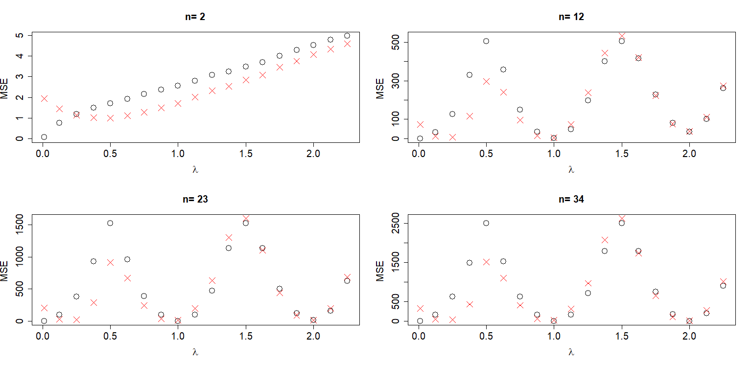
Figure 2: MSE as a function of $\lambda$ and fixed values of $n$. Circles represent $\operatorname{MSE}(U)$ while red x represent $\operatorname{MSE}(\hat{\theta})$.

The simulations indicate a periodic behavior of the $\operatorname{MSE}$ of $U$ and $\hat{\theta}$ as $\theta$ increases for most $n$, except $n=2$ (Figure 2). $\operatorname{MSE}(\hat{\theta})$ is generally smaller than $\operatorname{MSE}(U)$ until $\lambda\geq 1$, when $\operatorname{MSE}(\hat{\theta})$ is slightly bigger than $\operatorname{MSE}(U)$ most of the time. The exception is when $\lambda\approx 0$, when the MLE struggles to be close to $\theta$ (Theorem 6). There is evidence of oscillations in mean squared errors, with a dip when $\lambda$ is an integer. The peaks of the mean squared errors occur when $\lambda=1/2,3/2,...$; and at these values both mean squared errors become larger as $n\to\infty$.

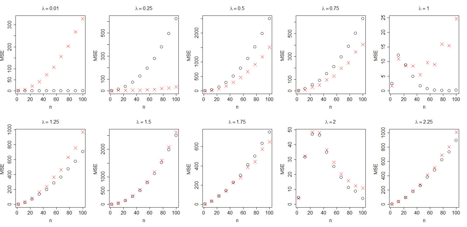
Figure 3: MSE as a function of $n$ and fixed values of $\lambda$. Circles represent $\operatorname{MSE}(U)$ while red x represent $\operatorname{MSE}(\hat{\theta})$.

In contrast, as a function of $n$ the mean squared errors generally increase (Figure 3). To see why, recall that $\operatorname{MSE}(U)=bias^{2}+\operatorname{Var}(U)$. While $\operatorname{Var}(U)\to 0$ as $n\to\infty$ (unless $\theta=I+0.5$), $bias^{2}$ tends to $(n[\lambda]-n\lambda)^{2}$. However, when $\lambda$ is a whole number, then the bias of $U$ tends to 0 as seen in the chart when $\lambda=1,\lambda=2$.

For $\lambda$ values close to 0 and large $n$ (first upper panel, Figure 3), $\hat{\theta}$ has a significantly larger mean squared error than $U$. This is because as $n\rightarrow\infty$, $\lceil u-\frac{n}{2}\rceil$ becomes smaller. This can cause the MLE to use as little as $n/2$ terms which will bias its result such that $\hat{\theta}>\theta$.

2.3 Binomial Distribution Case

We now consider the case where there are independent random variables $X_{k}\sim binomial(m,\phi)$, $Y=\sum_{k=1}^{n}X_{k}$ and the goal is to infer on $\phi$. Now $U$ has domain $u\in\{0,n,...,mn\}$. Once more, $U$ has effectively binned the possible values of $Y$.

Corollary 2.

If $Y\sim binomial(mn,\phi)$, $q=1-\phi$, $U=n[\frac{Y}{n}]$ and $\omega=exp(\frac{2\pi i}{n})$, then

$$\operatorname{E}(U) = mn\phi+\frac{1}{2}\left(2r-1\right)+\sum^{n-1}_{j=1}a(j)\frac{(1-\phi+\frac{\phi}{\omega^{j}})^{mn}}{1-\omega^{j}}$$

and

$$\operatorname{Var}(U) = mn\phi q+\frac{1}{12}(n^{2}-1)-\left(2mn\phi-1\right)\sum^{n-1}_{j=1}a(j)\frac{(q+\frac{\phi}{\omega^{j}})^{mn}}{1-\omega^{j}}$$

$$-\left(\sum^{n-1}_{j=1}a(j)\frac{(q+\frac{\phi}{\omega^{j}})^{mn}}{1-\omega^{j}}\right)^{2}-2\sum^{n-1}_{j=1}a(j)\left(\frac{mn\phi(q+\frac{\phi}{\omega^{j}})^{mn-1}}{1-\omega^{j}}-\frac{(q+\frac{\phi}{\omega^{j}})^{mn}}{\left(1-\omega^{j}\right)^{2}}\right)$$

where

$$r = \begin{cases}1\hskip 14.22636ptn\text{ is even}\\ 1/2\hskip 14.22636ptn\text{ is odd}\end{cases}$$

and

$$a(j) = \begin{cases}(-1)^{j}\hskip 14.22636ptn\text{ is even}\\ (-1)^{j}\omega^{j/2}\hskip 14.22636ptn\text{ is odd}\end{cases}$$

If $n=2$ then,

$$\operatorname{E}(U)=2m{\phi}+\dfrac{1}{2}+\frac{\left(1-2{\phi}\right)^{2m}}{2}$$

When $m=1$ in this scenario, $\operatorname{E}(U)=1+2\phi^{2}$ instead of $2\phi=\operatorname{E}(Y)$. The MLE of $\phi$ in terms of $U$ appears to have a complicated form and requires further research.

3 Example Applications

In this section we first consider the situation when we have estimated counts according to two averages rounded to the nearest non-negative integer coming from two separate time periods, and we wish to draw inference on the difference of the mean total counts. In a second application, the hidden random variable $Y$ follows a binomial distribution and the aim is to draw inference on the probability of success $\phi$. Lastly, we provide a framework to obtain the MLE based on $U$ when the underlying true count follows a Poisson, binomial or negative binomial distribution.

3.1 Estimating Excess Deaths Due to an Emergency

We now present an example of a rather simple before and after comparison to estimate excess deaths due to an emergency. Let $X\sim Poisson(\theta)$ represent the total deaths occurring in $n_{1}$ days before the emergency and $Y\sim Poisson(\theta+\beta)$ are the deaths in $n_{2}$ days after the emergency starts. $X$ and $Y$ are independent. $\beta$ measures excess deaths, a proxy of the impact of the emergency on mortality. A reasonable point estimator of excess deaths would be (Rivera and Rolke, 2018, 2019)

$$L^{*}\equiv(\bar{Y}-\bar{X})n_{2}=(Y-\frac{n_{2}}{n_{1}}X)$$ (11)

where $\bar{X}=\frac{X}{n_{1}}$ and $\bar{Y}=\frac{Y}{n_{2}}$. For this estimator,

$$\operatorname{E}(L^{*})=\beta+\theta\left(1-\frac{n_{2}}{n_{1}}\right)$$ (12)

and

$$\operatorname{Var}(L^{*})=\beta+\theta\left(1+\frac{n_{2}^{2}}{n_{1}^{2}}\right)$$ (13)

The second term makes adjustments to the moments dependent on the size of the before and after emergency sample sizes. However, when total counts must be estimated through averages rounded to the nearest non-negative integer, then the estimator becomes

$$([\bar{Y}]-[\bar{X}])n_{2}=U_{2}-[\bar{X}]n_{2}=\left(U_{2}-\frac{n_{2}}{n_{1}}U_{1}\right)\equiv L$$ (14)

That is, $U_{2}-U_{1}$ where $U_{1}=n_{1}[\frac{X}{n_{1}}]$, is only a suitable estimator when $n_{1}=n_{2}$. Our theoretical results shed light on the impact of supplanting (11) with (14). Now referring to Corollary 1 we have,

$$\operatorname{E}(L) = \beta+\theta\left(1-\frac{n_{2}}{n_{1}}\right)+\frac{1}{2}(2r_{2}-1)-\frac{n_{2}}{2n_{1}}(2r_{1}-1)+$$ (15)

$$e^{-\beta}\sum^{n_{1}-1}_{j=1}a_{1}(j)\frac{e^{\frac{\beta}{\omega_{1}^{j}}}}{1-\omega_{1}^{j}}-\frac{n_{2}e^{-(\theta+\beta)}}{n_{1}}\sum^{n_{2}-1}_{j=1}a_{2}(j)\frac{e^{\frac{(\theta+\beta)}{\omega_{2}^{j}}}}{1-\omega_{2}^{j}}$$

where $\omega_{k}=exp(\frac{2\pi k}{n_{k}})$ and

$$r_{k} = \begin{cases}1\hskip 14.22636ptn_{k}\text{ is even}\\ 1/2\hskip 14.22636ptn_{k}\text{ is odd}\end{cases}$$

and

$$a_{k}(j) = \begin{cases}(-1)^{j}\hskip 14.22636ptn_{k}\text{ is even}\\ (-1)^{j}\omega_{k}^{j/2}\hskip 14.22636ptn_{k}\text{ is odd}\end{cases}$$

Moreover,

$$\operatorname{Var}(L)=\beta+\theta\left(1+\frac{n_{2}^{2}}{n_{1}^{2}}\right)+\frac{n_{2}^{2}-1}{12}+\frac{n_{2}^{2}(n_{1}^{2}-1)}{12n_{1}^{2}}+Q_{1}$$ (16)

where $Q_{1}$ is a term resulting from the series in (8). Alternatively, $\widehat{\theta+\beta}-\frac{n_{2}}{n_{1}}\hat{\theta}$ can be used as an MLE estimator for $L^{*}$; where the first term is a function of $U_{2}$ and the second of $U_{1}$. Considering the application, it is reasonable to assume that $n_{1},n_{2}$ are not large. Rounding effects on the expected value of the estimator can be studied comparing (12) and (15), while rounding effects on estimator variance can be studied comparing (13) and (16). The main points are:

• If $\theta$ is large, then from (14) and Lemma 2 we have that $\operatorname{E}(L)\approx\operatorname{E}(L^{*})$ and $\operatorname{Var}(L)\approx\operatorname{Var}(L^{*})$.

• If $\theta$ is not large, $n_{1}$ is even and $n_{2}>2n_{1}$, then from (15) we see that $\operatorname{E}(L)$ will deviate considerably from $\operatorname{E}(L^{*})$. When $n_{2}>n_{1}$, (16) shows that $\operatorname{Var}(L)$ will deviate considerably from $\operatorname{Var}(L^{*})$ regardless of whether $n_{1}$ is even or odd. Moderate values of $n_{1}$ and $n_{2}$ would create a bias due to the third and fourth term in (16). The level of the bias is dependent on $\beta$ and $\theta$, which impact $Q_{1}$.

• As implied in section 2, if either $\theta$ or $\theta+\beta$ are of form $n_{k}(I+0.5)$, then $\operatorname{Var}(L)$ will be large. Both parameters having this form will result in a larger value of (16).

• Corollary 1 and Figure 2 imply that for $\theta+\beta\leq n_{2}/2$, $U_{2}$ will have a substantially larger $\operatorname{MSE}$ than the MLE of $\theta+\beta$. If $n_{1}=n_{2}$ and $\theta\leq n_{1}/2$, $U_{1}$ will have a substantially larger $\operatorname{MSE}$ than the MLE of $\theta$. This would lead to an overestimation of excess deaths unless $\theta+\beta\leq n_{2}/2$; when an underestimation may occur.

• When $\theta$ or $\theta+\beta$ are large, their respective MLEs $\hat{\theta}$, $\widehat{\theta+\beta}$ should perform well (Lemma 2).

3.2 Inference on probability of success $\phi$

Now consider a sequence of latent random variables $X_{k}\sim binomial(m,\phi)$, $k=1,..,n$ and our aim is to draw inference on $\phi$. Clearly, $Y=\sum_{k}X_{k}\sim binomial(mn,\phi)$. Corollary 2 demonstrates how moments of $U$ theoretically deviate from moments of $Y$ and section 2.3 gives an example where $\operatorname{E}(U)$, and $\operatorname{E}(Y)$ can be very different. In this section, we compare the true significance level when using $Y$ vs when we actually have $U=n[Y/n]$ available to examine the practical implications of the theoretical results presented. When using $U$, many analysts will draw inference on $\phi$ by misspecifying its distribution as $binomial(mn,\phi)$. Specifically, we will test

$$H_{o}:\phi=\phi_{o}\text{ vs. }H_{a}:\phi\neq\phi_{o}$$

with test statistic

$$T=\frac{w-mn\phi_{o}}{\sqrt{mn\phi_{o}(1-\phi_{o})}}$$

where the null is rejected at significance level $\alpha$ if $\mid T\mid$ is greater than the standardized score $z_{\alpha/2}$ and $w$ is either $y$ or $u$. The true significance level is (Casella and Berger, 2001)

$$P(W\leq mn\phi_{o}-z_{\alpha/2}\sqrt{mn(1-\phi_{o})})+P(W\geq mn\phi_{o}+z_{\alpha/2}\sqrt{mn(1-\phi_{o})})$$

To ensure the normal approximation is good we choose $m=500,n=31$ and values of $\phi_{o}$ between 0.1 and 0.9. Comparison was done based on 0.01, 0.05, and 0.1 nominal significance levels. The left panel of Figure 4 shows the true significance when $Y$ is available. The oscillatory behavior in true significance can be attributed to the lattice structure in $Y$ (Brown et al, 2001). When using $U$ and misspecifying its distribution as binomial, the true significance levels oscillate as a function of $\phi_{o}$ much more than when $Y$ is available, with values that can be far higher than the nominal significance level (right panel Figure 4). With $U$ the true significance value is always higher than the nominal $\alpha$.

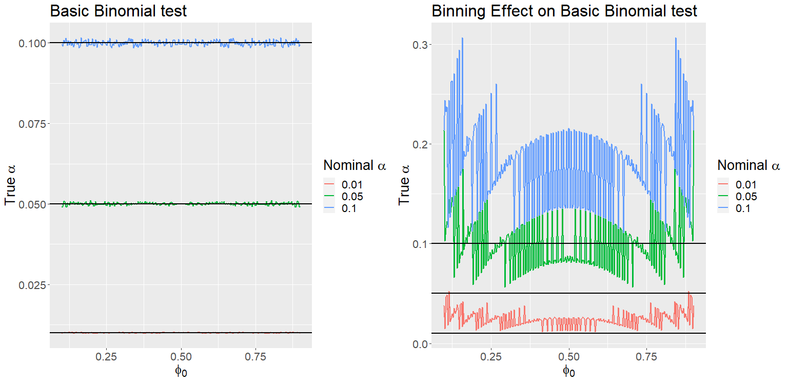
Figure 4: On the left we see the true significance level if $Y$ was available. On the right we have the true significance level when using $U$ and assuming it follows a binomial distribution.

Instead of misspecifying the distribution of $U$, Figure 5 shows the true significance level of $U$ when a binned binomial test is performed; where calculations are based on the pmf of $U$ according to Lemma 1. While the true significance value is now always lower than the nominal $\alpha$, the bias of the true significance level can be much smaller than when misspecifying the distribution of $U$. Still, the use of $U$ has caused the oscillations in interval coverage to be much more pronounced in comparison to using $Y$. For example, when the nominal significance level is 0.1, the true significance level of $U$ may be closer to 0.025 for some values $\phi_{o}$, and when the nominal significance level is 0.05, the true significance level of $U$ may be closer to 0.01 for some values $\phi_{o}$ (Figure 5). R code for the binned binomial test is available as supplementary material (R Core Team, 2020).

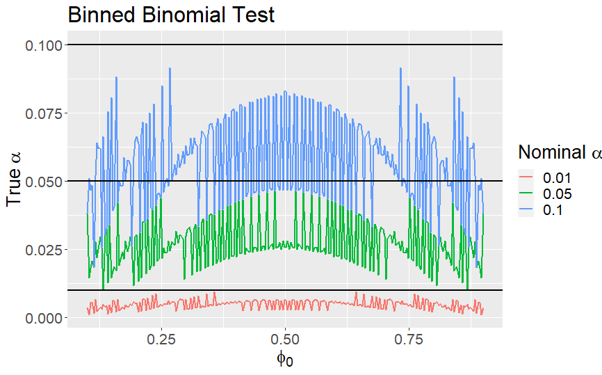
Figure 5: The true significance level when using $U$ with probability mass function as given in Lemma 1.

3.3 Numerical MLE

We can also measure the effect of rounding as the ratio of the mean squared errors of the maximum likelihood estimators of parameter $\nu$ with and without rounding:

$$\psi(\nu,n)=\frac{\operatorname{MSE}\left(\hat{\nu}(u(Y,n))\right)}{\operatorname{MSE}\left(\hat{\nu}(Y)\right)}=\frac{\operatorname{E}\left(\hat{\nu}(u(Y,n))-\nu\right)^{2}}{\operatorname{E}\left(\hat{\nu}(Y)-\nu\right)^{2}}$$

Because of the discrete nature of the distributions under consideration these mean squared errors can be found numerically. For the Poisson, Binomial or Negative Binomial distributions we proceed as follows (see R routine mse.ratio in supplementary material): (i) for a set of parameter values, find integers $y$ for which $\ignorespaces P(Y=y)>10^{-10}$ ; (ii) for these values $y$ find the MLE of the rounded number $u$ via numerical optimization of the log likelihood function; (iii) finally, to obtain $\psi(\nu,n)$ evaluate

$$\operatorname{E}\left(T(Y)-\nu\right)^{2}=\sum_{k=0}^{\infty}\left(T(k)-\nu\right)^{2}P(Y=k)\\$$

The result of the routine is either a graph of $\psi(\nu,n)$ or a list of the vectors with the mean squared errors and $\psi(\nu,n)$.

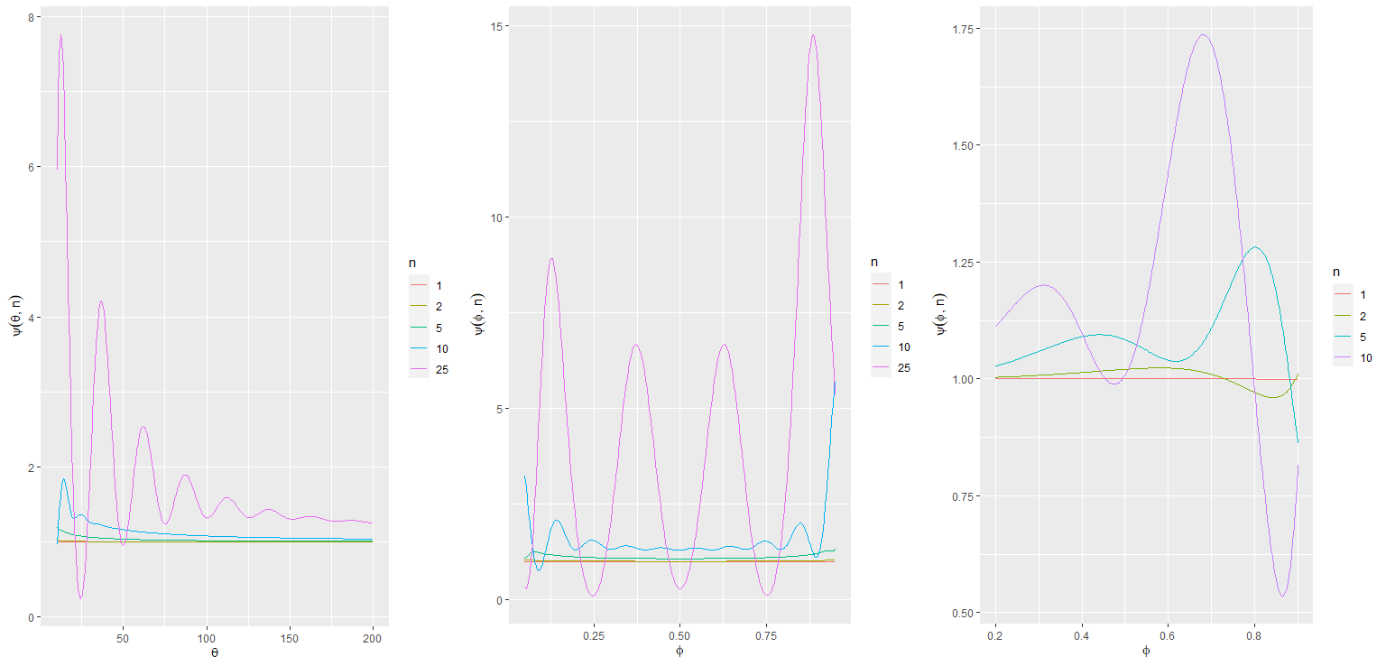
Figure 6: The mean squared errors of estimators based on $u$, $y$, and 5 sample sized when $Y$ follows a Poisson distribution (left), a binomial (middle) and negative binomial (right).

As examples, we consider $\psi(\nu,n)$ in the case of Poisson, binomial, and negative binomial $Y$ when $n=1,2,5,10,25$. For the Poisson case our aim is to estimate expected value $\theta$ and for the other two distributions, success probability $\phi$. When $Y$ follows a Poisson distribution, $\psi(\theta,n)$ is generally larger for small values of $\theta$. This makes sense as counts $u$ are biased to small values (left panel, Figure 6). Larger values of $n$ will make the ratio more pronounced and $\psi(\theta,n)$ will oscillate until $\theta$ is large enough. In the case of $Y$ following a binomial distribution, $\psi(\phi,n)$ oscillates with greater amplitude as $n$ increases (middle panel, Figure 6). When $n=25$, $\operatorname{MSE}\left(\hat{\phi}(u(Y,n))\right)>\operatorname{MSE}\left(\hat{\phi}(Y)\right)$ for some $\phi$ but for other $\phi$ $\operatorname{MSE}\left(\hat{\phi}(u(Y,n))\right)<\operatorname{MSE}\left(\hat{\phi}(Y)\right)$. Lastly, when $Y$ follows a negative binomial distribution, the right panel of Figure 6 also demonstrates possible large oscillations regardless of value of $\phi$. It should be noted that the results for the binomial and negative binomial will depend on the chosen parameter $N=nm$, and similarly, the Poisson chart will depend on the ratio between $n$ and $\theta$. Nevertheless, this example presents further evidence of rounding effects not being ignorable.

Importantly, the examples presented here show that in some cases rounding has an effect on estimating the parameter of interest regardless of sample size or parameter value.

4 Discussion

The explosion of data and the proposal of lower precision deep learning algorithms to speed up computations has made scientists rethink ignoring rounding error.

In this paper, we study the effects of relying on an average rounded to the nearest non-negative integer times $n$ measurements to get $U$ as a proxy of total counts. We derive expressions for $P(U=u),\operatorname{E}(U)$, and $\operatorname{Var}(U)$. As far as we know, this is the first time the effect of rounding is assessed for discrete random variables. Conditions when rounding error is negligible and when it is not, are presented. Most notably, if $X_{k}$ are iid non-negative discrete random variables with finite mean $\lambda$ and finite variance $\sigma^{2}$ we find that when $n$ is much larger than $\lambda$, $\operatorname{Var}(U)>>\operatorname{Var}(Y)$ when $\lambda\approx I+0.5$. Also, when $n$ is much larger than $\lambda$, fractional parts of $\lambda$ less than 0.5 will result in $\operatorname{E}(U)<<n\lambda$, and fractional parts greater than 0.5 will result in $\operatorname{E}(U)>>n\lambda$. For a long time it was considered that rounding had negligible consequences in statistical inference. Yet the alternating series found in $\operatorname{E}(U)$ and $\operatorname{Var}(U)$ can result in an oscillating behavior dependent on $n$ and parameter values; which can significantly alter statistical inference as the three examples demonstrate. Studies have reached similar conclusions assessing impact of rounding error on continuous variables and statistical inference Wang and Wertelecki (2013); Tricker et al (1998). As illustrated through the excess deaths example, rounding may result in significant first order bias as well. Equation (14) combined with the work from Janson (2006) may elucidate the influence of rounding when comparing means from two different continuous random variables.

We demonstrated how the use of the true pmf of $U$, helped reduce the bias in significance level calculations, albeit the bias may still be substantial. We also present a maximum likelihood estimator for the case of $Y\sim Poisson(\theta)$ and explore its theoretical properties. The MLE $\hat{\theta}$ performs well for most values of $\theta$ and $\operatorname{MSE}(\hat{\theta})$ is generally smaller than $\operatorname{MSE}(U)$ for small parameter values. Code to obtain numerical MLE when the underlying distribution is binomial or negative binomial is provided as supplementary material.

We did not explore methods that calibrate rounding errors. Future research includes following a Berkson measurement error model, such that a nonparametric estimator of the distribution of $Y$ could be constructed (Wang and Wertelecki, 2013). The optimal transport theory approach Peyré et al (2019) is another promising research path. Future work could examine the Wasserstein distance between the distributions of $U$ and $Y$, develop minimum Wasserstein distance estimators Bernton et al (2019) or approximating intractable $U$ distributions Torres et al (2021).

Author contributions

Conceptualization: Rivera; Methodology: Rivera, Cortes; Formal analysis and investigation: Rivera, Cortes, Reyes, Rolke; Writing - original draft preparation: Rivera, Cortes, Reyes; Writing - review and editing: Rivera; Supervision: Rivera.

Financial disclosure

None reported.

Conflict of interest

The authors declare no potential conflict of interests.

Supporting information

Additional supporting information may be found in the online version of the article at the publisher’s website.

Appendix A Proofs

A.1 Proof of Lemma 1

Proof:

It is straightforward to show that,

$$P(U=u)=P(n[\frac{Y}{n}]=u)=P([\frac{Y}{n}]=\frac{u}{n})$$

The pmf of $U$ depends on $n$. Specifically, when $n$ is odd then,

$$P(U=u) = P(u-\frac{n}{2}+\frac{1}{2}\leq Y\leq u+\frac{n}{2}-\frac{1}{2})\hskip 28.45274pt\text{Since }Y\text{ must be an integer}$$

$$= \sum_{q=g(u)}^{n-1}P(Y=u-\frac{n}{2}+\frac{1}{2}+q)\hskip 56.9055ptu\in\{0,n,2n,..\}$$

Assuming $n$ is even then things get a bit more complicated, mainly because the pmf will depend on the type of of tie breaking rule used (a tie is when the fraction of the average is 0.5). If the round half to even rule is used, then

$$P(U=u) = P(\frac{u}{n}-0.5\leq\frac{Y}{n}<\frac{u}{n}+0.5)$$

$$= \begin{cases}\sum_{q=0}^{n}P(Y=u-\frac{n}{2}+q)&u/n\text{ is even}\\ \sum_{q=0}^{n-2}P(Y=u-\frac{n}{2}+1+q)&u/n\text{ is odd}\\ \end{cases}$$

where $u\in\{0,n,2n,..\}$. When $u=0,n\geq 2$, then $u-\frac{n}{2}+q<0$, and $P(Y=u-\frac{n}{2}+q)=0$ until $q\geq\frac{n}{2}$. Alternatively we may use a round half up tie breaking rule,

$$P(U=u) = P([\frac{Y}{n}]=\frac{u}{n})=P(\lfloor\frac{Y}{n}+0.5\rfloor=\frac{u}{n})$$

$$= P(\frac{u}{n}\leq\frac{Y}{n}+0.5<\frac{u}{n}+1)=P(\frac{u}{n}-0.5\leq\frac{Y}{n}<\frac{u}{n}+0.5)$$

$$= P(u-\frac{n}{2}\leq Y<u+\frac{n}{2})=\sum_{q=g(u)}^{n-1}P(Y=u-\frac{n}{2}+q)$$

Adjusting the summation index to start at zero completes the proof.

A.2 Proof of Theorem 1

Proof: For even $n$,

$$G_{U}(s) = (p_{0}+\cdots+p_{\frac{n}{2}-1})+(p_{\frac{n}{2}}+\cdots+p_{n+\frac{n}{2}-1})s^{n}+(p_{n+\frac{n}{2}}+\cdots+p_{2n+\frac{n}{2}-1})s^{2n}+\cdots$$ (17)

$$+(p_{(m-1)n+\frac{n}{2}}+\cdots+p_{mn+\frac{n}{2}-1})s^{mn}+\cdots$$

$$= \sum_{k=0}^{n/2-1}p_{k}+\sum_{l=0}^{\infty}\sum_{k=0}^{n-1}p_{n/2+ln+k}s^{n/2+ln}$$

Recall that the sum of the pgf converges for any $s\in{\rm I\!R}$ such that $\mid s\mid\leq 1$. Meanwhile, we may write $G_{Y}(s)$ as

$$G_{Y}(s)=\sum_{k=0}^{n/2-1}p_{k}s^{k}+\sum_{l=0}^{\infty}\sum_{k=0}^{n-1}p_{n/2+ln+k}s^{n/2+ln+k}.$$ (18)

Next, we transform (18) the following way,

$$\omega^{jn/2}G_{Y}(s/\omega^{j}) = \sum_{k=0}^{n/2-1}p_{k}s^{k}\omega^{j(n/2-k)}+\sum_{l=0}^{\infty}\sum_{k=0}^{n-1}p_{n/2+ln+k}s^{n/2+ln+k}\omega^{-j(ln+k)}$$ (19)

$$= \sum_{k=0}^{n/2-1}p_{k}s^{k}\omega^{j(n/2-k)}+\sum_{l=0}^{\infty}\sum_{k=0}^{n-1}p_{n/2+ln+k}s^{n/2+ln+k}\omega^{-jk}$$

where the second equality is due to $\omega^{-jln}=1$, for integer values of $j$. The inverse discrete Fourier transform of this function is

$$\frac{1}{n}\sum_{j=0}^{n-1}\omega^{j\left(\frac{n}{2}+q\right)}G_{Y}\left(\frac{s}{\omega^{j}}\right) = \frac{1}{n}\sum_{j=0}^{n-1}(-1)^{j}\omega^{jq}G_{Y}\left(\frac{s}{\omega^{j}}\right)$$ (20)

$$= p_{q-n/2}s^{q-n/2}+\sum_{l=0}^{\infty}p_{\frac{n}{2}+ln+q}s^{\frac{n}{2}+ln+q},$$

where $p_{k}=0$, for any $k<0$.

The probability generating function for $U$ can then be written as,

$$G_{U}(s) = \sum_{q=0}^{n/2-1}p_{q}+\sum_{l=0}^{\infty}\sum_{q=0}^{n-1}p_{n/2+ln+q}s^{n+ln}$$ (21)

$$= \sum_{q=0}^{n-1}\left(s^{n/2-q}\frac{1}{n}\sum_{j=0}^{n-1}\omega^{jq}(-1)^{j}G_{Y}(s/\omega^{j})\right)$$

$$= \frac{s^{n}-1}{ns^{n/2-1}}\sum_{j=0}^{n-1}(-1)^{j}\frac{G_{Y}\left(\frac{s}{\omega^{j}}\right)}{s-\omega^{j}},$$

where the last equality follows from resumming the $q$-dependent terms as a geometric series.

For odd $n$

$$G_{U}(s)=\operatorname{E}(s^{U})=(p_{0}+\cdots+p_{\frac{n}{2}-\frac{1}{2}})+(p_{\frac{n}{2}+\frac{1}{2}}+\cdots+p_{n+\frac{n}{2}-\frac{1}{2}})s^{n}+\cdots$$

and following a similar procedure as for even sample we get,

$$G_{U}(s) = \sum_{q=0}^{n/2-1/2}p_{q}+\sum_{l=0}^{\infty}\sum_{q=0}^{n-1}p_{n/2+1/2+ln+q}s^{n+ln}$$

$$= \sum_{q=0}^{n-1}\left(s^{n/2+1/2-q}\frac{1}{n}\sum_{j=0}^{n-1}\omega^{j(q+1/2)}(-1)^{j}G_{Y}(s/\omega^{j})\right)$$

$$= \frac{s^{n}-1}{ns^{(n-1)/2}}\sum_{j=0}^{n-1}(-1)^{j}\frac{\omega^{j/2}G_{Y}\left(\frac{s}{\omega^{j}}\right)}{s-\omega^{j}}$$

A.3 Proof of Theorem 2

We will consider the version of $G_{U}(s)$ free of pole singularity at $s=1$; thus for $j=0$ in (3) we have:

$$\frac{s^{n}-1}{s-1}$$

a finite geometric series (when $s\neq 1$) and therefore:

$$G_{U}(s) = \frac{1}{n}\left(G_{Y}(s)\sum_{t=0}^{n-1}s^{t+r-\frac{n}{2}}+\frac{s^{n}-1}{s^{\frac{n}{2}-r}}\sum^{n-1}_{j=1}a(j)\frac{G_{Y}(s/\omega^{j})}{s-\omega^{j}}\right)$$

Taking the derivative with respect to $s$ we have:

$$nG^{\prime}_{U}(s) = \frac{G_{Y}(s)}{2}\sum_{t=1}^{n}(2r-2+2t-n)s^{r-2+t-\frac{n}{2}}+G_{Y}^{{}^{\prime}}(s)\sum_{t=1}^{n}s^{r-1+t-\frac{n}{2}}+$$ (23)

$$\frac{1}{2}\Bigl{(}(n+2r)s^{\frac{n}{2}+r-1}-(-n+2r)s^{-\frac{n}{2}+r-1}\Bigr{)}\sum^{n-1}_{j=1}a(j)\frac{G_{Y}(\frac{s}{\omega^{j}})}{s-\omega^{j}}+$$

$$\left(s^{\frac{n+2r}{2}}-s^{\frac{-n+2r}{2}}\right)\sum^{n-1}_{j=1}a(j)\left(\frac{G_{Y}^{{}^{\prime}}(\frac{s}{\omega^{j}})}{\omega^{j}(s-\omega^{j})}-\frac{G_{Y}(\frac{s}{\omega^{j}})}{\left(s-\omega^{j}\right)^{2}}\right)$$

Thus, at $s=1$ we get:

$$nG^{\prime}_{U}(1) = \frac{1}{2}G_{Y}(1)\left(2r-1\right)n+nG_{Y}^{{}^{\prime}}(1)+n\sum^{n-1}_{j=1}a(j)\frac{G_{Y}(\frac{1}{\omega^{j}})}{1-\omega^{j}}$$ (24)

Lastly, recall that $G_{Y}(1)=\sum_{k=0}^{\infty}p_{k}=1$.

A.3.1 Proof for $\operatorname{Var}(U)$

From equation (23):

$$nG^{{}^{\prime\prime}}_{U}(s) = \frac{1}{4}G_{Y}(s)\sum^{n}_{t=1}(2r-4-n+2t)(2r-2-n+2t)s^{r-3-\frac{n}{2}+t}$$

$$+\frac{1}{2}G_{Y}^{{}^{\prime}}(s)\sum^{n}_{t=1}s^{r-2-\frac{n}{2}+t}+\frac{1}{2}G_{Y}^{{}^{\prime}}(s)\sum^{n}_{t=1}(2r-2-n+2t)s^{r-1-\frac{n}{2}+t}$$

$$+\sum^{n}_{t=1}s^{r-1-\frac{n}{2}+t}G_{Y}^{{}^{\prime\prime}}(s)+\frac{1}{4}(n+2r-2)(n+2r)s^{\frac{n}{2}+r-1}$$

$$-\frac{1}{4}(-n+2r-2)(-n+2r)s^{-\frac{n}{2}+r-1}\sum^{n-1}_{j=1}a(j)\frac{G_{Y}(\frac{s}{\omega^{j}})}{s-\omega^{j}}$$

$$+\frac{1}{2}\leavevmode\resizebox{422.77661pt}{}{$\Bigl{(}(n+2r)s^{\frac{n}{2}+r-1}-(-n+2r)s^{-\frac{n}{2}+r-1}\Bigr{)}\sum^{n-1}_{j=1}a(j)\left(\frac{G_{Y}^{{}^{\prime}}(\frac{s}{\omega^{j}})}{\omega^{j}(s-\omega^{j})}-\frac{G_{Y}(\frac{s}{\omega^{j}})}{(s-\omega^{j})^{2}}\right)$}$$

$$+\frac{1}{2}\leavevmode\resizebox{422.77661pt}{}{$\Bigl{(}(n+2r)s^{\frac{n+2r}{2}}-(-n+2r)s^{\frac{-n+2r}{2}}\Bigr{)}\sum^{n-1}_{j=1}a(j)\left(\frac{G_{Y}^{{}^{\prime}}(\frac{s}{\omega^{j}})}{\omega^{j}(s-\omega^{j})}-\frac{G_{Y}(\frac{s}{\omega^{j}})}{(s-\omega^{j})^{2}}\right)$}$$

$$+\left(s^{\frac{n+2r}{2}}-s^{\frac{-n+2r}{2}}\right)\sum^{n-1}_{j=1}a(j)\left(\frac{G_{Y}^{{}^{\prime\prime}}(\frac{s}{\omega^{j}})}{\omega^{2j}(s-\omega^{j})}-2\frac{G_{Y}^{{}^{\prime}}(\frac{s}{\omega^{j}})}{\omega^{j}(s-\omega^{j})^{2}}+2\frac{G_{Y}(\frac{s}{\omega^{j}})}{\left(s-\omega^{j}\right)^{3}}\right)$$

Which leads to:

$$nG^{{}^{\prime\prime}}_{U}(1) = \frac{1}{4}G_{Y}(1)\sum^{n}_{t=1}(2r-4-n+2t)(2r-2-n+2t)$$ (25)

$$+G_{Y}^{{}^{\prime}}(1)\sum^{n}_{t=1}(2r-2-n+2t)+nG_{Y}^{{}^{\prime\prime}}(1)$$

$$+\frac{1}{4}(4n)\left(2r-1\right)\sum^{n-1}_{j=1}a(j)\frac{G_{Y}(\frac{1}{\omega^{j}})}{1-\omega^{j}}+2n\sum^{n-1}_{j=1}a(j)\left(\frac{G_{Y}^{{}^{\prime}}(\frac{1}{\omega^{j}})}{\omega^{j}(1-\omega^{j})}-\frac{G_{Y}(\frac{1}{\omega^{j}})}{\left(1-\omega^{j}\right)^{2}}\right)$$

$$= (r^{2}+\frac{n^{2}}{4}-rn-3r+\frac{3n}{2}+2)n+(4r-2n-6)\frac{n(n+1)}{4}$$

$$+\frac{n(n+1)(2n+1)}{6}G_{Y}(1)+(2r-1)nG_{Y}^{{}^{\prime}}(1)+nG_{Y}^{{}^{\prime\prime}}(1)$$

$$+n\left(2r-1\right)\sum^{n-1}_{j=1}a(j)\frac{G_{Y}(\frac{1}{\omega^{j}})}{1-\omega^{j}}+2n\sum^{n-1}_{j=1}a(j)\left(\frac{G_{Y}^{{}^{\prime}}(\frac{1}{\omega^{j}})}{\omega^{j}(1-\omega^{j})}-\frac{G_{Y}(\frac{1}{\omega^{j}})}{\left(1-\omega^{j}\right)^{2}}\right)$$

$$= \frac{n}{12}\left(n^{2}+12r^{2}-24r+8\right)G_{Y}(1)+(2r-1)nG_{Y}^{{}^{\prime}}(1)+nG_{Y}^{{}^{\prime\prime}}(1)+$$

$$n\left(2r-1\right)\sum^{n-1}_{j=1}a(j)\frac{G_{Y}(\frac{1}{\omega^{j}})}{1-\omega^{j}}+2n\sum^{n-1}_{j=1}a(j)\left(\frac{G_{Y}^{{}^{\prime}}(\frac{1}{\omega^{j}})}{\omega^{j}(1-\omega^{j})}-\frac{G_{Y}(\frac{1}{\omega^{j}})}{\left(1-\omega^{j}\right)^{2}}\right)$$

and

$$G^{{}^{\prime\prime}}_{U}(1) = \frac{1}{12}\left(n^{2}+12r^{2}-24r+8\right)+(2r-1)\operatorname{E}(Y)+G_{Y}^{{}^{\prime\prime}}(1)+$$

$$\left(2r-1\right)\sum^{n-1}_{j=1}a(j)\frac{G_{Y}(\frac{1}{\omega^{j}})}{1-\omega^{j}}+2\sum^{n-1}_{j=1}a(j)\left(\frac{G_{Y}^{{}^{\prime}}(\frac{1}{\omega^{j}})}{\omega^{j}(1-\omega^{j})}-\frac{G_{Y}(\frac{1}{\omega^{j}})}{\left(1-\omega^{j}\right)^{2}}\right)$$

Therefore $\operatorname{Var}(U)=G^{\prime\prime}_{U}(1)+\operatorname{E}(U)-(\operatorname{E}(U))^{2}$ becomes

$$\operatorname{Var}(U) = G_{Y}^{{}^{\prime\prime}}(1)+\operatorname{E}(Y)-(\operatorname{E}(Y))^{2}+\frac{1}{12}(n^{2}-1)-\left(2\operatorname{E}(Y)-1\right)\sum^{n-1}_{j=1}a(j)\frac{G_{Y}(\frac{1}{\omega^{j}})}{1-\omega^{j}}$$

$$-\left(\sum^{n-1}_{j=1}a(j)\frac{G_{Y}(\frac{1}{\omega^{j}})}{1-\omega^{j}}\right)^{2}+2\sum^{n-1}_{j=1}a(j)\left(\frac{G_{Y}^{{}^{\prime}}(\frac{1}{\omega^{j}})}{\omega^{j}(1-\omega^{j})}-\frac{G_{Y}(\frac{1}{\omega^{j}})}{\left(1-\omega^{j}\right)^{2}}\right)$$

$$= \operatorname{Var}(Y)+\frac{1}{12}(n^{2}-1)-\left(2\operatorname{E}(Y)-1\right)\sum^{n-1}_{j=1}a(j)\frac{G_{Y}(\frac{1}{\omega^{j}})}{1-\omega^{j}}$$

$$-\left(\sum^{n-1}_{j=1}a(j)\frac{G_{Y}(\frac{1}{\omega^{j}})}{1-\omega^{j}}\right)^{2}+2\sum^{n-1}_{j=1}a(j)\left(\frac{G_{Y}^{{}^{\prime}}(\frac{1}{\omega^{j}})}{\omega^{j}(1-\omega^{j})}-\frac{G_{Y}(\frac{1}{\omega^{j}})}{\left(1-\omega^{j}\right)^{2}}\right)$$

A.4 Proof of Corollary 1

For $\operatorname{E}(U)$ simply replace in (7) $G_{Y}(1/\omega^{j})$ and $\operatorname{E}(Y)$ by their respective values when $Y\sim Poisson(\theta)$.

For $\operatorname{Var}(U)$ replace in (8) $G_{Y}(1/\omega^{j}),G_{Y}^{{}^{\prime}}(1/\omega^{j}),\operatorname{E}(Y),\operatorname{Var}(Y)$ by their respective values when $Y\sim Poisson(\theta)$ leads to

$$\operatorname{Var}(U) = \theta+\frac{1}{12}(n^{2}-1)-e^{-2\theta}\left(\sum^{n-1}_{j=1}a(j)\frac{e^{\frac{\theta}{\omega^{j}}}}{1-\omega^{j}}\right)^{2}$$

$$-e^{-\theta}(2\theta-1)\sum^{n-1}_{j=1}a(j)\frac{e^{\frac{\theta}{\omega^{j}}}}{1-\omega^{j}}$$

$$+2e^{-\theta}\sum^{n-1}_{j=1}a(j)\frac{e^{\frac{\theta}{\omega^{j}}}}{1-\omega^{j}}\left(\theta-\frac{1}{1-\omega^{j}}\right)$$

Re-expressing algebraically the answer is obtained.

A.5 Proof of Lemma 2

Proof: In terms of the probabilities $p_{k}$, according to (17) and (A.2) $\operatorname{E}(U)$ is given by,

$$\operatorname{E}(U)=\sum_{l=0}^{\infty}\sum_{q=0}^{n-1}(n+ln)p_{n/2+a+ln+q}$$

where $a=0$ if $n$ is even and $a=1/2$ is $n$ is odd. At large values of $\lambda$, the Poisson probabilities are approximated by a Gaussian distribution as,

$$\operatorname{E}(U)\to\sum_{l=0}^{\infty}\sum_{q=0}^{n-1}(n+ln)\frac{e^{-(n/2+a+ln+q-\theta)^{2}/2\theta}}{\sqrt{2\pi\theta}}$$

We define the new variable $x=n/2+a+ln+q$, such that

$$\operatorname{E}(U)\to J_{1}-J_{2}-J_{3}-J_{4}$$

where,

$$J_{1} \equiv \sum_{x=0}^{\infty}x\,\frac{e^{-(x-\theta)^{2}/2\theta}}{\sqrt{2\pi\theta}},$$

$$J_{2} \equiv \sum_{x=0}^{n/2+a}x\,\frac{e^{-(x-\theta)^{2}/2\theta}}{\sqrt{2\pi\theta}},$$

$$J_{3} \equiv \sum_{l=0}^{\infty}\sum_{q=0}^{n-1}(a-n/2)\frac{e^{-(n/2+a+ln+q-\theta)^{2}/2\theta}}{\sqrt{2\pi\theta}},$$

$$J_{4} \equiv \sum_{l=0}^{\infty}\sum_{q=0}^{n-1}q\frac{e^{-(n/2+a+ln+q-\theta)^{2}/2\theta}}{\sqrt{2\pi\theta}}$$

The first sum is a standard Poisson-expected value calculation, such that $J_{1}=\theta$.

For the second sum we can place an upper bound by substituting each term in the sum with the highest value of $x=n/2+a$,

$$J_{2}<(n/2+a)^{2}\frac{e^{-(n/2+a-\theta)^{2}/2\theta}}{\sqrt{2\pi\theta}}$$

which vanishes exponentially if $\theta\gg n/2+a$. The third integral is simply,

$$J_{3}=(a-n/2)\sum_{x=0}^{\infty}\frac{e^{-(x-\theta)^{2}/2\theta}}{\sqrt{2\pi\theta}}=(a-n/2)$$

For the fourth integral we can again place an upper bound, by replacing in each term in the sum over $q$ with its highest value,

$$J_{4}<(n-1)\sum_{l=0}^{\infty}\sum_{q=0}^{n-1}\frac{e^{-(n/2+a+ln+q-\theta)^{2}/2\theta}}{\sqrt{2\pi\theta}}=(n-1)$$

Then it is easy to show,

$$\lim_{\lambda\to\infty}\frac{1}{n\lambda}\operatorname{E}(U)=\lim_{\lambda\to\infty}\frac{1}{n\lambda}(J_{1}+J_{2}+J_{3}+J_{4})=\lim_{\Lambda\to\infty}\frac{1}{n\lambda}J_{1}=1$$

Now we turn to the variance, which can be written in the large $\lambda$ limit as

$$\operatorname{Var}(U) = \sum_{l=0}^{\infty}\sum_{q=0}^{n-1}(n+ln)^{2}\frac{e^{-(n/2+a+ln+q-\theta)^{2}/2\theta}}{\sqrt{2\pi\theta}}$$

$$-\left(\sum_{l=0}^{\infty}\sum_{q=0}^{n-1}(n+ln)\frac{e^{-(n/2+a+ln+q-\theta)^{2}/2\theta}}{\sqrt{2\pi\theta}}\right)^{2}$$

Again we define $x=n/2+a+ln+q$. such that

$$\operatorname{Var}(U)=J_{1}-J_{2}-J_{3}-J_{4}+J_{5}-J_{6}+J_{7}$$

where,

$$J_{1} \equiv \sum_{x=0}^{\infty}x^{2}\,\frac{e^{-(x-\theta)^{2}/2\theta}}{\sqrt{2\pi\theta}}-\left(\sum_{x=0}^{\infty}x\,\frac{e^{-(x-\theta)^{2}/2\theta}}{\sqrt{2\pi\theta}}\right)^{2}$$

$$J_{2} \equiv \sum_{x=0}^{n/2+a}x^{2}\,\frac{e^{-(x-\theta)^{2}/2\theta}}{\sqrt{2\pi\theta}}-\left(\sum_{x=0}^{n/2+a}x\,\frac{e^{-(x-\theta)^{2}/2\theta}}{\sqrt{2\pi\theta}}\right)^{2}$$

$$J_{3} \equiv \sum_{l=0}^{\infty}\sum_{q=0}^{n-1}2x(n/2-a-q)\frac{e^{-(n/2+a+ln+q-\theta)^{2}/2\theta}}{\sqrt{2\pi\theta}},$$

$$J_{4} \equiv \sum_{l=0}^{\infty}\sum_{q=0}^{n-1}(n/2-a-q)^{2}\frac{e^{-(n/2+a+ln+q-\theta)^{2}/2\theta}}{\sqrt{2\pi\theta}},$$

$$J_{5} \equiv \left(\sum_{0}^{\infty}2x\frac{e^{-(x-\theta)^{2}/2\theta}}{\sqrt{2\pi\theta}}\right)\left(\sum_{l=0}^{\infty}\sum_{q=0}^{n-1}(n/2-a-q)\frac{e^{-(n/2+a+ln+q-\theta)^{2}/2\theta}}{\sqrt{2\pi\theta}}\right),$$

$$J_{6} \equiv \left(\sum_{0}^{x=n/2+a}2x\frac{e^{-(x-\theta)^{2}/2\theta}}{\sqrt{2\pi\theta}}\right)\left(\sum_{l=0}^{\infty}\sum_{q=0}^{n-1}(n/2-a-q)\frac{e^{-(n/2+a+ln+q-\theta)^{2}/2\theta}}{\sqrt{2\pi\theta}}\right),$$

$$J_{7} \equiv \left(\sum_{l=0}^{\infty}\sum_{q=0}^{n-1}(n/2-a-q)\frac{e^{-(n/2+a+ln+q-\theta)^{2}/2\theta}}{\sqrt{2\pi\theta}}\right)^{2}$$

The first expression is the standard Poisson variance $J_{1}=\theta$. We again find bounds for the rest of the sums,

$$J_{2} < (n/2+a)^{3}\frac{e^{-(n/2+a-\theta)^{2}/2\theta}}{\sqrt{2\pi\theta}}-\left((n/2+a)^{2}\frac{e^{-(n/2+a-\theta)^{2}/2\theta}}{\sqrt{2\pi\theta}}\right)^{2}$$

$$J_{4} < (n/2-a-n+1)^{2}$$

$$J_{6} < 2(n/2-a+1)(n/2-a)^{2}(n-1)\frac{e^{-(n/2-a-\theta)^{2}/2\theta}}{\sqrt{2\pi\theta}}$$

$$J_{7} < (n/2-a-n+1)^{2}$$

and,

$$J_{3}-J_{5}=\sum_{l=0}^{\infty}\sum_{q=0}^{n-1}(2\theta-n/2+a+ln+q)q\frac{e^{-(n/2+a+ln+q-\theta)^{2}/2\theta}}{\sqrt{2\pi\theta}}.$$ (26)

In expression (26) we define the new variable $y=ln/\theta$, and for large $\lambda$ we approximate the sum over $l$ with an integral over $y$,

$$J_{3}-J_{5}\approx\frac{\theta}{n}\int_{0}^{\infty}\sum_{q=0}^{n-1}2\theta(1-n/2\theta-a/\theta-y-q/\theta)q\,\frac{e^{-\theta(n/2\theta+a/\theta+y+q/\theta-1)^{2}/2}}{\sqrt{2\pi\theta}}dy$$

At large $\lambda$, the integral over $y$ can be calculated with a saddle point approximation, where the saddle point is given by $y_{sp}=1-n/2\theta-a/\theta-q/\theta$, resulting in,

$$J_{3}-J_{5}\to 0+\mathcal{O}\left(\frac{1}{\sqrt{\theta}}\right)$$

Putting all these results together we then find,

$$\lim_{\lambda\to\infty}\frac{1}{n\lambda}\operatorname{Var}(U)=\lim_{\lambda\to\infty}\frac{1}{n\lambda}J_{1}=1$$

A.6 Proof for Theorem 3

Proof:

From (2.1) we see that for $n>1$ the log-likelihood is,

$$l = \log(L(\theta\mid u))=(h(u)+g(u))\log(\theta)-\theta+\log(\sum_{q=0}^{n-1-g(u)}\frac{\theta^{q}}{(h(u)+g(u)+q)!})$$

$$= c\log(\theta)-\theta+\log(\sum_{q=0}^{n-1-g(u)}d_{q}\theta^{q})$$

where $c=h(u)+g(u)$ and $d_{q}=\frac{1}{(c+q)!}$. Then

$$\frac{d\log l}{d\theta} = \frac{c}{\theta}-1+\frac{\sum_{q=1}^{n-1-g(u)}d_{q}q\theta^{q-1}}{\sum_{q=0}^{n-1-g(u)}d_{q}\theta^{q}}=0$$

$$= \frac{c-\theta}{\theta}+\frac{\sum_{q=1}^{n-1-g(u)}d_{q}q\theta^{q-1}}{\sum_{q=0}^{n-1-g(u)}d_{q}\theta^{q}}=0$$

$$= \frac{c\sum_{q=0}^{n-1-g(u)}d_{q}\theta^{q}-\theta\sum_{q=0}^{n-1-g(u)}d_{q}\theta^{q}+\theta\sum_{q=1}^{n-1-g(u)}d_{q}q\theta^{q-1}}{\theta\sum_{q=0}^{n-1-g(u)}d_{q}\theta^{q}}=0$$

$$= c\sum_{q=0}^{n-1-g(u)}d_{q}\theta^{q}-\theta\sum_{q=0}^{n-1-g(u)}d_{q}\theta^{q}+\theta\sum_{q=1}^{n-1-g(u)}d_{q}q\theta^{q-1}=0$$

$$= c\sum_{q=0}^{n-1-g(u)}d_{q}\theta^{q}-\sum_{q=0}^{n-1-g(u)}d_{q}\theta^{q+1}+\sum_{q=1}^{n-1-g(u)}d_{q}q\theta^{q}=0$$

$$= c\sum_{q=0}^{n-1-g(u)}d_{q}\theta^{q}-\sum_{q=1}^{n-1+1-g(u)}d_{q-1}\theta^{q}+\sum_{q=1}^{n-1-g(u)}d_{q}q\theta^{q}=0$$

$$= cd_{0}-d_{n-1}\theta^{n-1+1-g(u)}+c\sum_{q=1}^{n-1-g(u)}d_{q}\theta^{q}-\sum_{q=1}^{n-1-g(u)}(c+q)d_{q}\theta^{q}+$$

$$\sum_{q=1}^{n-1-g(u)}d_{q}q\theta^{q}=0$$

$$= cd_{0}-d_{n-1}\theta^{n-1+1}=0$$

The equality before last occurs because $d_{q-1}=(c+q)d_{q}$. Therefore,

$$\hat{\theta} = (\frac{cd_{0}}{d_{n-1}})^{1/(n-1+1)}=\Bigl{(}(h(u)+g(u)+n-1)....(h(u)+g(u))\Bigr{)}^{1/n}$$

$$= \begin{cases}\Bigl{(}(u-\frac{n}{2}+\frac{1}{2}+g(u)+n-1)...(u-\frac{n}{2}+\frac{1}{2}+g(u))\Bigr{)}^{\frac{1}{n}}\hskip 14.22636ptn\text{ is odd}\\ \Bigl{(}(u+\frac{n}{2}-1+g(u))....(u-\frac{n}{2}+g(u))\Bigr{)}^{\frac{1}{n}}\hskip 14.22636ptn\text{ is even}\end{cases}$$

$$= \begin{cases}\prod_{q=0}^{n-1-g(u)}\Bigl{(}u-\frac{n}{2}+\frac{1}{2}+g(u)+q\Bigr{)}^{\frac{1}{n}}\hskip 14.22636ptn\text{ is odd}\\ \prod_{q=0}^{n-1-g(u)}\Bigl{(}u-\frac{n}{2}+g(u)+q\Bigr{)}^{\frac{1}{n}}\hskip 14.22636ptn\text{ is even}\\ \end{cases}$$

$$= \prod_{q=0}^{n-1-g(u)}\Bigl{(}\lceil u-\frac{n}{2}\rceil+g(u)+q\Bigr{)}^{\frac{1}{n}}$$

This MLE adjusts for the effect of rounding to the nearest integer. Occasions when $\lceil u-\frac{n}{2}\rceil+g(u)+q<0$ are of probability zero and thus must be omitted before calculating the geometric mean,

$$\hat{\theta} = \prod_{q\in\mathcal{P}}\Bigl{(}\lceil u-\frac{n}{2}\rceil+g(u)+q\Bigr{)}^{\frac{1}{m}}$$

where $\mathcal{P}$ is the set such that $\lceil u-\frac{n}{2}\rceil+g(u)+q>0$ and $m$ is the length of $\mathcal{P}$.

A.7 Proof of Theorem 4

Proof:

Considering large $\lambda$ we omit $g(u)$ from (9),

$$\operatorname{E}(\hat{\theta})=\sum_{u/n=0}^{\infty}\prod_{k\in\mathcal{P}}\Bigl{(}\lceil u-n/2\rceil+k\Bigr{)}^{\frac{1}{m}}P(U=u)$$

At large $\lambda$, with (17) and (A.2) we use the fact that $P(Y=y)$ is approximately Gaussian, and we can express the expectation value as,

$$\operatorname{E}(\hat{\theta})=\sum_{l=0}^{\infty}\sum_{q=0}^{n-1}\prod_{k\in\mathcal{P}}(ln-n/2+a)\prod_{k\in\mathcal{P}}\left(1+\frac{k}{ln-n/2+a}\right)^{\frac{1}{m}}\frac{e^{-(ln+n/2+a+q-\theta)^{2}/2\theta}}{\sqrt{2\pi\theta}}$$

where $a=0$ if $n$ is even and $a=1/2$ is $n$ is odd. The Gaussian distribution for large $\lambda$ implies that the only contributions to the sum that are not exponentially small are where $ln\sim\theta$, therefore we can assume $ln\gg n,a,k,q$, in the expression for $\operatorname{E}(\hat{\theta})$ and,

$$\operatorname{E}(\hat{\theta})\approx\sum_{l=0}^{\infty}\sum_{q=0}^{n-1}ln\prod_{k=0}^{n-1}\left(1+\frac{k}{ln}\right)^{\frac{1}{n-1}}\frac{e^{-(ln+n/2+a+q-\theta)^{2}/2\theta}}{\sqrt{2\pi\theta}}$$

where since we exclude the probability that $l=0$, now all $\mathcal{P}$ are of the same size $n-1$. Furthermore, since $k\ll ln$, we can approximate,

$$\operatorname{E}(\hat{\theta}) \approx \sum_{l=0}^{\infty}\sum_{q=0}^{n-1}ln\frac{e^{-(ln+n/2+a+q-\theta)^{2}/2\theta}}{\sqrt{2\pi\theta}}$$

$$= \operatorname{E}(U)-\sum_{l=0}^{\infty}\sum_{q=0}^{n-1}n\frac{e^{-(ln+n/2+a+q-\theta)^{2}/2\theta}}{\sqrt{2\pi\theta}}$$

Now invoking Lemma 2, we find

$$\lim_{\lambda\to\infty}\frac{1}{n\lambda}\operatorname{E}(\hat{\theta})=\lim_{\lambda\to\infty}\frac{1}{n\lambda}\left(\operatorname{E}(U)-n\right)=1$$

A.8 Proof of Theorem 5

Proof:

The expected value of the MLE is given by,

$$\operatorname{E}(\hat{\theta})=\sum_{u/n=0}^{\infty}\prod_{k\in\mathcal{P}}\left(\lceil u-n/2\rceil+k\right)^{\frac{1}{m}}P(U=u)$$

where we express the sum in terms of $u/n$ which has a non-negative integers support. From Lemma 1, for large $n$ we have $v_{0}=\lfloor\lambda+0.5\rfloor$ and $P(U=u)\approx\delta^{\rm Kronecker}_{u,nv_{0}}$, so

$$\lim_{n\to\infty}\operatorname{E}(\hat{\theta})=\lim_{n\to\infty}\prod_{k=0}^{n-1}(\lceil nv_{0}-n/2\rceil+k)^{\frac{1}{n}}=\lim_{n\to\infty}\lceil nv_{0}-n/2\rceil\prod_{k=0}^{n-1}\left(1+\frac{k}{\lceil nv_{0}-n/2\rceil}\right)^{\frac{1}{n}}$$

In the large $n$ limit, It is more convenient to work with the logarithm of $\operatorname{E}(\hat{\theta})$,

$$\lim_{n\to\infty}\log(\operatorname{E}(\hat{\theta}))=\lim_{n\to\infty}\left[\log(\lceil nv_{0}-n/2\rceil)+\sum_{k=0}^{n-1}\frac{1}{n}\log\left(1+\frac{k}{\lceil nv_{0}-n/2\rceil}\right)\right]$$

In the large $n$ limit, the sum over $k$ can be approximated with an integral over variable $x=k/\lceil nv_{0}-n/2\rceil$,

$$\lim_{n\to\infty}\log(\operatorname{E}(\hat{\theta})) = \lim_{n\to\infty}\left[\log(\lceil nv_{0}-n/2\rceil)+\frac{\lceil nv_{0}-n/2\rceil}{n}\int_{0}^{\frac{n-1}{\lceil nv_{0}-n/2\rceil}}\log(1+x)dx\right]$$

$$= \lim_{n\to\infty}\left[\log(\lceil nv_{0}-n/2\rceil)+\Bigl{(}v_{0}-\frac{1}{2}\Bigr{)}\Bigl{(}\frac{1}{v_{0}-\frac{1}{2}}+1\Bigr{)}\log\left(\frac{1}{v_{0}-1/2}+1\right)-1\right]$$

Exponentiating both sides and dividing by $n$ we get our result (10).

A.9 Proof of Theorem 6

Proof:

Observe that in the large $n$ limit, probability mass concentrates more in $u=0$, such that

$$\lim_{n\to\infty}\operatorname{E}(\hat{\theta})=\lim_{n\to\infty}\prod_{k=n/2}^{n-1}(\lceil-n/2\rceil+k)^{2/n}=\lim_{n\to\infty}\frac{n}{2}\prod_{k=n/2}^{n-1}\left(-1+\frac{2k}{n}\right)^{2/n}$$

We now take the logarithm on both sides, such that

$$\lim_{n\to\infty}\log(\operatorname{E}(\hat{\theta}))=\lim_{n\to\infty}\left[\log\left(\frac{n}{2}\right)+\sum_{k=n/2}^{n-1}\frac{2}{n}\log\left(-1+\frac{2k}{n}\right)\right]$$

where the sum can be approximated by an integral in the large $n$ limit as,

$$\lim_{n\to\infty}\log(\operatorname{E}(\hat{\theta}))=\lim_{n\to\infty}\left[\log\left(\frac{n}{2}\right)+\int_{1}^{2}\log\left(-1+x\right)dx\right]=\log\left(\frac{n}{2}\right)-1$$

Exponentiating both sides of the equation, and dividing by $n$, we have,

$$\lim_{n\to\infty}\frac{1}{n}\operatorname{E}(\hat{\theta})=\frac{1}{2e}$$

A.10 Proof for Corollary 2

For $\operatorname{E}(U)$ simply replace $G_{Y}(1/\omega^{j})$ and $\operatorname{E}(Y)$ by their respective values when

$Y\sim binomial(mn,\phi)$.

For $\operatorname{Var}(U)$:

$$\begin{split}nG^{\prime\prime}_{U}(s)=&\frac{mn\phi}{2}\left(q+\phi s\right)^{mn-1}\sum^{n}_{t=1}(2r-n-2+2t)s^{r-2+t-\frac{n}{2}}+\\ &\frac{1}{2}\left((q+\phi s)^{m}n-q^{m}n\right)\sum^{n}_{t=1}\left(r-2+t-\frac{n}{2}\right)\left(2r-n-2+2t\right)s^{r-3+t-\frac{n}{2}}+\\ &mn(mn-1)\phi^{2}\left(q+\phi s\right)^{mn-2}\sum^{n}_{t=1}s^{r-1+t-\frac{n}{2}}+\\ &mn\phi\left(q+\phi s\right)^{mn-1}\sum^{n}_{t=1}\left(r-1+t-\frac{n}{2}\right)s^{r-2+t-\frac{n}{2}}\\ &+\frac{1}{2}(\left(\frac{n}{2}+r-1\right)\left(n+2r\right)s^{\frac{n}{2}+r-2}\\ &-\left(-\frac{n}{2}+r-1\right)\left(-n+2r\right)s^{-\frac{n}{2}+r-2})\sum^{n-1}_{j=1}\frac{(q+\frac{\phi s}{\omega^{j}})^{mn}-q^{mn}}{s-\omega^{j}}\\ &\leavevmode\resizebox{422.77661pt}{}{$+\left((n+2r)s^{\frac{n+2r-2}{2}}-(-n+2r)s^{\frac{-n+2r-2}{2}}\right)\sum^{n-1}_{j=1}\left(\frac{\frac{mn\phi}{\omega^{j}}(q+\frac{\phi s}{\omega^{j}})^{mn-1}}{s-\omega^{j}}-\frac{(q+\frac{\phi s}{\omega^{j}})^{mn}-q^{mn}}{\left(s-\omega^{j}\right)^{2}}\right)$}\\ &\leavevmode\resizebox{422.77661pt}{}{$+\left(s^{\frac{n+2r}{2}}-s^{\frac{-n+2r}{2}}\right)\sum^{n-1}_{j=1}(\frac{mn(mn-1)\left(\frac{\phi}{\omega^{j}}\right)^{2}(q+\frac{\phi s}{\omega^{j}})^{mn-2}}{s-\omega^{j}}-2\frac{\frac{mn\phi}{\omega^{j}}(q+\frac{\phi s}{\omega^{j}})^{mn-1}}{\left(s-\omega^{j}\right)^{2}}$}\\ &+2\frac{(q+\frac{\phi s}{\omega^{j}})^{mn}-q^{mn}}{\left(s-\omega^{j}\right)^{3}})\end{split}$$

Thus, $nG^{\prime\prime}_{U}(1)$ is given by:

$$nG^{\prime\prime}_{U}(1) = \frac{mn\phi}{2}n\left(2r-1\right)+\frac{n}{12}\left(n^{2}+12r^{2}-24r+8\right)\left(1-q^{mn}\right)$$

$$+mn(mn-1)n\phi^{2}+(r-\frac{1}{2})mn^{2}\phi$$

$$-n\left(2r-1\right)\sum^{n-1}_{j=1}\frac{(q+\frac{\phi}{\omega^{j}})^{mn}-q^{mn}}{\omega^{j}-1}$$

$$-2n\sum^{n-1}_{j=1}\left(\frac{\frac{mn\phi}{\omega^{j}}(q+\frac{\phi}{\omega^{j}})^{mn-1}}{\omega^{j}-1}+\frac{(q+\frac{\phi}{\omega^{j}})^{mn}-q^{mn}}{\left(\omega^{j}-1\right)^{2}}\right)$$

Some additional algebraic calculations lead to the result.

References

- \bibcommenthead
- Beath et al (2012) Beath C, Becerra-Fernandez I, Ross J, et al (2012) Finding value in the information explosion. MIT Sloan Management Review 53(4):18
- Bernton et al (2019) Bernton E, Jacob PE, Gerber M, et al (2019) On parameter estimation with the wasserstein distance. Information and Inference: A Journal of the IMA 8(4):657–676
- Brown et al (2001) Brown LD, Cai TT, DasGupta A (2001) Interval estimation for a binomial proportion. Statistical Science pp 101–117
- Canoui-Poitrine et al (2006) Canoui-Poitrine F, Cadot E, Spira A (2006) Excess deaths during the august 2003 heat wave in paris, france. Revue d’épidémiologie et de santé publique 54(2):127–135
- Casella and Berger (2001) Casella G, Berger RL (2001) Statistical inference
- Chen (2021) Chen T (2021) Non-asymptotic moment bounds for random variables rounded to non-uniformly spaced sets. Stat p e395
- Colangelo et al (2018) Colangelo P, Nasiri N, Nurvitadhi E, et al (2018) Exploration of low numeric precision deep learning inference using intel® fpgas. In: 2018 IEEE 26th annual international symposium on field-programmable custom computing machines (FCCM), IEEE, pp 73–80
- Gupta et al (2015) Gupta S, Agrawal A, Gopalakrishnan K, et al (2015) Deep learning with limited numerical precision. In: International conference on machine learning, PMLR, pp 1737–1746
- Hooten et al (2011) Hooten MB, Leeds WB, Fiechter J, et al (2011) Assessing first-order emulator inference for physical parameters in nonlinear mechanistic models. Journal of Agricultural, Biological, and Environmental Statistics 16(4):475–494
- Janson (2006) Janson S (2006) Rounding of continuous random variables and oscillatory asymptotics. The Annals of Probability 34(5):1807–1826
- Kishore et al (2018) Kishore N, Marqués D, Mahmud A, et al (2018) Mortality in puerto rico after hurricane maria. New England Journal of Medicine
- Kutner et al (2009) Kutner NG, Muntner P, Huang Y, et al (2009) Effect of hurricane katrina on the mortality of dialysis patients. Kidney international 76(7):760–766
- Kutz (2013) Kutz JN (2013) Data-driven modeling & scientific computation: methods for complex systems & big data
- Lugo and Rivera (2023) Lugo O, Rivera R (2023) A closer look at indirect causes of death after hurricane maria using a semiparametric model. Disaster Medicine and Public Health Preparedness 17:e528. 10.1017/dmp.2023.165
- Pace et al (2004) Pace L, Salvan A, Ventura L (2004) The effects of rounding on likelihood procedures. Journal of Applied Statistics 31(1):29–48
- Peyré et al (2019) Peyré G, Cuturi M, et al (2019) Computational optimal transport: With applications to data science. Foundations and Trends® in Machine Learning 11(5-6):355–607
- Raissi et al (2017) Raissi M, Perdikaris P, Karniadakis GE (2017) Physics informed deep learning (part i): Data-driven solutions of nonlinear partial differential equations. arXiv preprint arXiv:171110561
- Rao et al (2020) Rao C, Sun H, Liu Y (2020) Physics-informed deep learning for incompressible laminar flows. Theoretical and Applied Mechanics Letters 10(3):207–212
- R Core Team (2020) R Core Team (2020) R: A Language and Environment for Statistical Computing. R Foundation for Statistical Computing., Vienna, Austria
- Resnick (1992) Resnick SI (1992) Adventures in stochastic processes
- Rivera (2020) Rivera R (2020) Principles of managerial statistics and data science
- Rivera and Rolke (2018) Rivera R, Rolke W (2018) Estimating the death toll of hurricane maria. Significance 15(1):8–9
- Rivera and Rolke (2019) Rivera R, Rolke W (2019) Modeling excess deaths after a natural disaster with application to hurricane maria. Statistics in medicine 38(23):4545–4554
- Rivera et al (2019) Rivera R, Marazzi M, Torres-Saavedra PA (2019) Incorporating open data into introductory courses in statistics. Journal of Statistics Education 27(3):198–207
- Rivera et al (2020) Rivera R, Rosenbaum JE, Quispe W (2020) Excess mortality in the united states during the first three months of the covid-19 pandemic. Epidemiology & Infection 148
- Rodriguez et al (2018) Rodriguez A, Segal E, Meiri E, et al (2018) Lower numerical precision deep learning inference and training. Intel White Paper 3:1–19
- Rosenbaum et al (2021) Rosenbaum JE, Stillo M, Graves N, et al (2021) Timeliness of us mortality data releases during the covid-19 pandemic: delays are associated with electronic death registration system and elevated weekly mortality. medRxiv
- Santos-Burgoa et al (2018) Santos-Burgoa C, Sandberg J, Suárez E, et al (2018) Differential and persistent risk of excess mortality from hurricane maria in puerto rico: a time-series analysis. The Lancet Planetary Health 2(11):e478–e488
- Santos-Lozada and Howard (2018) Santos-Lozada AR, Howard JT (2018) Use of death counts from vital statistics to calculate excess deaths in puerto rico following furricane maria. Jama 320(14):1491–1493
- Schneeweiß et al (2010) Schneeweiß H, Komlos J, Ahmad AS (2010) Symmetric and asymmetric rounding: a review and some new results. AStA Advances in Statistical Analysis 94(3):247–271
- Sheppard (1898) Sheppard WF (1898) On the calculation of the most probable values of frequency-constants, for data arranged according to equidistant division of a scale. Proceedings of the London Mathematical Society 1(1):353–380
- Stephens et al (2007) Stephens KU, Grew D, Chin K, et al (2007) Excess mortality in the aftermath of hurricane katrina: A preliminary report. Disaster Medicine and Public Health Preparedness 1(1):15–20. 10.1097/DMP.0b013e3180691856
- Taraldsen (2011) Taraldsen G (2011) Analysis of rounded exponential data. Journal of Applied Statistics 38(5):977–986
- Tilley et al (2019) Tilley A, Wilkinson SP, Kolding J, et al (2019) Nearshore fish aggregating devices show positive outcomes for sustainable fisheries development in timor-leste. Frontiers in Marine Science p 487
- Tong et al (2010) Tong S, Ren C, Becker N (2010) Excess deaths during the 2004 heatwave in brisbane, australia. International journal of biometeorology 54(4):393–400
- Torres et al (2021) Torres LC, Pereira LM, Amini MH (2021) A survey on optimal transport for machine learning: Theory and applications. arXiv preprint arXiv:210601963
- Tricker (1990) Tricker A (1990) The effect of rounding on the significance level of certain normal test statistics. Journal of Applied Statistics 17(1):31–38
- Tricker et al (1998) Tricker A, Coates E, Okell E (1998) The effect on the r chart of precision of measurement. Journal of Quality Technology 30(3):232–239
- Tricker (1984) Tricker AR (1984) Effects of rounding on the moments of a probability distribution. The Statistician pp 381–390
- Wang and Wertelecki (2013) Wang B, Wertelecki W (2013) Density estimation for data with rounding errors. Computational Statistics & Data Analysis 65:4–12
- Wang et al (2018) Wang N, Choi J, Brand D, et al (2018) Training deep neural networks with 8-bit floating point numbers. In: Proceedings of the 32nd International Conference on Neural Information Processing Systems, pp 7686–7695
- White (1982) White H (1982) Maximum likelihood estimation of misspecified models. Econometrica: Journal of the econometric society pp 1–25
- Wikle and Hooten (2010) Wikle CK, Hooten MB (2010) A general science-based framework for dynamical spatio-temporal models. Test 19(3):417–451
- Zhao and Bai (2020) Zhao N, Bai Z (2020) Bayesian statistical inference based on rounded data. Communications in Statistics-Simulation and Computation 49(1):135–146