Deep calibration of the quadratic rough Heston model

Abstract

The quadratic rough Heston model provides a natural way to encode Zumbach effect in the rough volatility paradigm. We apply multi-factor approximation and use deep learning methods to build an efficient calibration procedure for this model. We show that the model is able to reproduce very well both SPX and VIX implied volatilities. We typically obtain VIX option prices within the bid-ask spread and an excellent fit of the SPX at-the-money skew. Moreover, we also explain how to use the trained neural networks for hedging with instantaneous computation of hedging quantities.

Keywords— Quadratic rough Heston, multi-factor approximation, SPX smile, VIX smile, deep learning, joint calibration, hedging

1 Introduction

The rough volatility paradigm introduced in [13] is now widely accepted, both by practitioners and academics. On the macroscopic side, rough volatility models can fit with remarkable accuracy the shape of implied volatility smiles and at-the-money skew curves. They also reproduce amazingly well stylized facts of realized volatilities, see for example [3, 5, 8, 13, 23]. On the microstructural side, it is shown in [6, 7, 22] that the rough Heston model introduced and developed in [9, 10] naturally emerges from agents behaviors at the microstructural scale.

Nevertheless, one stylized fact of financial time series that is not reflected in the rough Heston model is the feedback effect of past price trends on future volatility, which is discussed by Zumbach in [24]. Super-Heston rough volatility models introduced in [6] fill this gap by considering quadratic Hawkes processes from microstructural level, and showing that the Zumbach effect remains explicit in the limiting models. As a particular example of super-Heston rough volatility models, the authors in [14] propose the quadratic rough Heston model, and show its promising ability to calibrate jointly SPX smiles and VIX smiles, where other continuous-time models have been struggling for a long time [17].

The VIX index is in fact by definition a derivative of the SPX index $S$, which can be represented as

$$\text{VIX}_{t}=\sqrt{-2\mathbb{E}[\log(S_{t+\Delta}/S_{t})|\mathcal{F}_{t}]}\times 100\,,$$ (1.1)

where $\Delta=30$ days and $\mathbb{E}$ is the risk-neutral expectation. Consequently, VIX options are also derivatives of SPX. Finding a model which jointly calibrates the prices of SPX and VIX options is known to be very challenging, especially for short maturities. As indicated in [17], “the very negative skew of short-term SPX options, which in continuous models implies a very large volatility of volatility, seems inconsistent with the comparatively low levels of VIX implied volatilities”. Through numerical examples, the authors in [14] show the relevance of the quadratic rough Heston model in terms of pricing simultaneously SPX and VIX options. In this paper, in the spirit of [2], we propose a multi-factor approximated version of this model and an associated efficient calibration procedure.

Under the rough Heston model, the characteristic function of the log-price has semi-closed form formula, and thus fast numerical pricing methods can be designed, see [10]. However, pricing in the quadratic rough Heston model is more intricate. The multi-factor approximation method for the rough kernel function developed in [2] makes rough volatility models Markovian in high dimension. Thus Monte-Carlo simulations become more feasible in practice. Still, in our case, model calibration remains a difficult task. Inspired by recent works about applications of deep learning in quantitative finance, see for example [4, 19, 20], we use deep neural networks to speed up model calibration. The effectiveness of the calibrated model for fitting jointly SPX and VIX smiles is illustrated through numerical experiments. Interestingly, under our model, the trained networks also allow us to hedge options with instantaneous computation of hedging quantities.

The paper is organized as follows. In Section 2, we give the definition of our model and introduce the approximation method. In Section 3, we develop the model calibration with deep neural networks. Validity of the methods is tested both on simulated data and market data. Finally in Section 4, we show how to perform hedging in the model with neural networks through some toy examples.

2 The quadratic rough Heston model and its multi-factor approximation

The quadratic rough Heston model, proposed in [14], for the price of an asset $S$(here the SPX) and its spot variance $V$ under risk-neutral measure is

$$dS_{t}=S_{t}\sqrt{V_{t}}dW_{t},\qquad V_{t}=a(Z_{t}-b)^{2}+c\,,$$ (2.1)

where $W$ is a Brownian motion, $a,b,c$ are all positive constants and $Z_{t}$ is defined as

$$Z_{t}=\int_{0}^{t}\lambda\frac{(t-s)^{\alpha-1}}{\Gamma(\alpha)}\big{(}\theta_{0}(s)-Z_{s}\big{)}ds+\int_{0}^{t}\eta\frac{(t-s)^{\alpha-1}}{\Gamma(\alpha)}\sqrt{V_{s}}dW_{s}\,,$$ (2.2)

for $t\in[0,T]$. Here $T$ is a positive time horizon, $\alpha\in(1/2,1)$, $\lambda>0$, $\eta>0$ and $\theta_{0}(\cdot)$ is a deterministic function. $Z_{t}$ is driven by the returns through $\sqrt{V_{t}}dW_{t}=dS_{t}/S_{t}$. Then the square in $V_{t}$ can be understood as a natural way to encode the so called strong Zumbach effect, which means that the conditional law of future volatility depends not only on path volatility trajectory but also on past returns. Note that in this case we have a pure-feedback model as $S_{t}$ and $V_{t}$ are driven by the same Brownian motion, see [6] for more details on the derivation of this type of models. We will see in Section 4 that this setting enables us to hedge perfectly European options with SPX only. We recall the parameter interpretation given in [14]:

• $a$ stands for the strength of the feedback effect on volatility.

• $b$ encodes the asymmetry of the feedback effect. It reflects the empirical fact that negative price returns can lead to volatility spikes, while it is less pronounced for positive returns.

• $c$ is the base level of variance, independent from past prices information.

It is shown in [10] that under the rough Heston model the volatility trajectories have almost surely H$\ddot{\text{o}}$lder regularity $\alpha-1/2-\varepsilon$, for any $\varepsilon>0$. This actually recalls the observation in [13] that the dynamic of log-volatility is similar to that of a fractional Brownian motion with Hurst parameter of order 0.1. Similarly the fractional kernel $K(t)=\frac{t^{\alpha-1}}{\Gamma(\alpha)}$ in (2.2) enables us to generate rough volatility dynamics, which is highly desirable as explained in the introduction. However, it makes the quadratic rough Heston model non-Markovian and non-semimartingale, and thus difficult to simulate efficiently. In this paper, we apply the multi-factor approximation proposed in [2] to do so. The key idea is to write the fractional kernel $K(t)$ as the Laplace transform of a positive measure $\mu$

$$K(t)=\int_{0}^{\infty}e^{-\gamma t}\mu(d\gamma),\quad\mu(d\gamma)=\frac{\gamma^{-\alpha}}{\Gamma(\alpha)\Gamma(1-\alpha)}d\gamma\,.$$

Then we approximate $\mu$ by a finite sum of Dirac measures $\mu^{n}=\sum_{i=1}^{n}c_{i}^{n}\delta_{\gamma_{i}^{n}}$ with positive weights $(c_{i}^{n})_{i=1,\cdots,n}$ and discount coefficients $(\gamma_{i}^{n})_{i=1,\cdots,n}$, with $n\geq 1$. This gives us the approximated kernel function

$$K^{n}(t)=\sum_{i=1}^{n}c_{i}^{n}e^{-\gamma^{n}_{i}t},\quad n\geq 1\,.$$

A well-chosen parametrization of the $2n$ parameters $(c^{n}_{i},\gamma^{n}_{i})_{i=1,\cdots,n}$ in terms of $\alpha$ can make $K^{n}(t)$ converge to $K(t)$ in the $L^{2}$ sense as $n$ goes to infinity, and the multi-factor approximation models behave closely to their counterparts in the rough volatility paradigm, see [1, 2] for more details. We recall in Appendix A the parametrization method proposed in [1]. Then given the time horizon $T$ and $n$, $(c^{n}_{i})_{i=1,\cdots,n}$ and $(\gamma^{n}_{i})_{i=1,\cdots,n}$ are just deterministic functions of $\alpha$, and therefore not free parameters to calibrate. We can give the following multi-factor approximation of the quadratic rough Heston model:

$$dS^{n}_{t} =S^{n}_{t}\sqrt{V^{n}_{t}}dW_{t},\quad V^{n}_{t}=a(Z^{n}_{t}-b)^{2}+c\,\,,$$ (2.3)

$$Z^{n}_{t} =\sum_{i=1}^{n}c^{n}_{i}Z^{n,i}_{t}\,\,,$$ (2.4)

$$dZ^{n,i}_{t} =(-\gamma^{n}_{i}Z^{n,i}_{t}-\lambda Z^{n}_{t})dt+\eta\sqrt{V^{n}_{t}}dW_{t},\qquad Z^{n,i}_{0}=z^{i}_{0}\,,$$ (2.5)

with $(z^{i}_{0})_{i=1,\cdots,n}$ some constants. Contrary to the case of the rough Heston model, $\theta(t)$ cannot be easily written as a functional of the forward variance curve in the quadratic rough Heston model. Then instead of making the factors $(Z^{n,i})_{i=1,\cdots,n}$ starting from 0 and taking $Z_{t}^{n}=\lambda\sum_{i=1}^{n}c_{i}^{n}\int_{0}^{t}e^{-\gamma_{i}^{n}(t-s)}\theta(s)ds+\sum_{i=1}^{n}c^{n}_{i}Z_{t}^{n,i}$, as the authors do in [1, 2], here we discard $\theta(\cdot)$ in Equation (2.4) and consider the starting values of factors $(z^{i}_{0})_{i=1,\cdots,n}$ as free parameters to calibrate from market data. This setting allows $Z_{0}$ and $V_{0}$ to adapt to market conditions and also encodes various possibilities for the “term-structure” of $Z^{n}_{t}$. To see this, given a solution for (2.3)-(2.5), (2.5) can be rewritten as

$$Z^{n,i}_{t}=z_{0}^{i}e^{-\gamma^{n}_{i}t}+\int_{0}^{t}e^{-\gamma^{n}_{i}(t-s)}\big{(}-\lambda Z^{n}_{s}ds+\eta\sqrt{V^{n}_{s}}dW_{s}\big{)}\,.$$ (2.6)

Then from (2.4) we can get

$$Z^{n}_{t}=g^{n}(t)+\int_{0}^{t}K^{n}(t-s)\big{(}b(Z^{n}_{s})ds+\sigma(Z^{n}_{s})dW_{s}\big{)}\,,$$ (2.7)

with $g^{n}(t)=\sum_{i=1}^{n}z^{i}_{0}c^{n}_{i}e^{-\gamma_{i}^{n}t}$, $b(Z^{n}_{t})=-\lambda Z^{n}_{t}$ and $\sigma(Z^{n}_{t})=\eta\sqrt{a(Z^{n}_{t}-b)^{2}+c}$. By taking expectation on both sides of (2.7), we get

$$\mathbb{E}[Z_{t}^{n}]+\lambda\sum_{i=1}^{n}c_{i}^{n}\int_{0}^{t}e^{-\gamma_{i}(t-s)}\mathbb{E}[Z_{s}^{n}]ds=\sum_{i=1}^{n}z_{0}^{i}c_{i}^{n}e^{-\gamma^{n}_{i}t}\,.$$

Thus we can see that the $(z^{i}_{0})_{i=1,\cdots,n}$ allows us to encode initial “term-structure” of $Z_{t}^{n}$. Therefore, it can be understood as an analogy of $\theta(t)$ for the variance process in the rough Heston model. Besides, we will see in Section 4 that this setting allows us to hedge options perfectly with only SPX.

By virtue of Proposition B.3 in [2], for given $n$, Equations (2.7) and equivalently (2.6) admit a unique strong solution, since $g^{n}(t)$ is H$\ddot{\text{o}}$lder continuous, $b(\cdot)$ and $\sigma(\cdot)$ have linear growth, and $K^{n}$ is continuously differentiable admitting a resolvent of the first kind. We stress again the fact that Model (2.3-2.5) does not bring new parameters to calibrate compared to the quadratic rough Heston model defined in (2.1-2.2), with the idea of the correspondance between $\theta(t)$ and $(z^{i}_{0})_{i=1,\cdots,n}$. The fractional kernel in the rough volatility paradigm helps us to build the factors $(Z^{n,i})_{i=1,\cdots,n}$. Factors with large discount coefficient $\gamma^{n}_{i}$ can mimic roughness and account for short timescales, while ones with small $\gamma^{n}_{i}$ capture information from longer timescales. The quantity $Z^{n}$ aggregates these factors and therefore encodes the multi-timescales nature of volatility processes, which is discussed for example in [11, 13].

Remark 2.1.

With multi-factor approximation, Model (2.3-2.5) is Markovian with a state vector of dimension $n+1$ given by $\mathbf{X}^{n}_{t}:=(S^{n}_{t},Z^{n,1}_{t},\cdots,Z^{n,n}_{t})$. Hence the price of SPX options at time $t$ is fully determined by $\mathbf{X}^{n}_{t}$.

As discussed in Appendix A, we choose $n=10$ in our numerical experiments. To simplify notations, we discard the label $n$ in the following, and let $\boldsymbol{\omega}:=(\lambda,\eta,a,b,c)\in\Omega\subset R^{5}$, $\mathbf{z}_{0}:=(z^{1}_{0},\cdots,z^{10}_{0})\in\mathcal{Z}\subset R^{10}$.

3 Model calibration with deep learning

The Markovian nature of Model (2.3-2.5) makes the calibration with Monte-Carlo simulations more feasible. However, besides parameters $\boldsymbol{\omega}$, the initial state of factors $\mathbf{z}_{0}$ is also supposed to be calibrated from market data. In this case pricing with Monte-Carlo is not well adapted to classical optimal parameter search methods for model calibration, as it leads to heavy computation and the results are not always satisfactory. To bypass this “curse of dimensionality”, we apply deep learning to speed up further model calibration. Deep learning has already achieved remarkable success with high-dimensional data like images and audio. Recently its potentials for model calibration in quantitative finance has been investigated for example in [4, 19, 20]. Two types of methods are proposed in the literature:

• From prices to model parameters (PtM) [19]: deep neural networks are trained to approximate the mapping from prices of some financial contracts, e.g. options, to model parameters. With this method, we can get directly the calibrated parameters from market data, without use of some numerical methods searching for optimal parameters.

• From model parameters to prices (MtP) [4, 20]: in the first step, deep neural networks are trained to approximate the pricing function, that is the mapping from model parameters to prices of financial contracts. Then in the second step, traditional optimization algorithms can be used to find optimal parameters, to minimize the discrepancy between market data and model outputs.

It is hard to say that one method is always better than the other. PtM method is faster and avoids computational errors caused by optimization algorithms, while MtP method is more robust to the varying nature of options data (strike, maturity, $\ldots$). In the following, the two methods are applied with implied volatility surfaces (IVS), represented by certain points with respect to some predetermined strikes and maturities. During model calibration, all these points need to be built from market quotes for PtM method, while we could focus on some points of interest for MtP method, for example those near-the-money. For comparison, we will test both methods in the following with simulated data.

3.1 Methodology

The neural networks used in our tests are all multilayer perceptrons. They are trained with synthetic dataset generated from the model. Our methodology is mainly based on two steps: data generation and model training.

- Synthetic data generation

The objective is to generate data samples $\big{\{}\boldsymbol{\omega},\mathbf{z}_{0},IVS_{SPX},IVS_{VIX}\big{\}}$, where $IVS_{SPX}$ and $IVS_{VIX}$ stand for implied volatility surface of SPX and VIX options respectively. We randomly sample $\boldsymbol{\omega}$ and $\mathbf{z}_{0}$ with the following distribution:

$$\boldsymbol{\omega} \in\mathcal{U}[0.5,2.5]\times\mathcal{U}[1.0,1.5]\times\mathcal{U}[0.1,0.6]\times\mathcal{U}[0.01,0.5]\times\mathcal{U}[0.0001,0.03]\,,$$

$$\mathbf{z}_{0} \in\mathcal{U}[-0.5,0.5]^{10}\,,\text{where }\mathcal{U}\text{ denotes the uniform distribution}\,.$$

For each sampling from above distribution, we generate 50,000 random paths of SPX and VIX with the explicit-implicit Euler scheme (A.1). Then Monte-Carlo prices are used to compute $IVS_{SPX}^{MC}$ and $IVS_{VIX}^{MC}$ with respect to some predetermined log-moneyness strikes and maturities:

• log-moneyness strikes of SPX options: $k_{SPX}$ = {-0.15, -0.12, -0.1, -0.08, -0.05, -0.04, -0.03, -0.02, -0.01, 0.0, 0.01, 0.02, 0.03, 0.04, 0.05},

• log-moneyness strikes of VIX options: $k_{VIX}$ = {-0.1, -0.05, -0.03, -0.01, 0.01, 0.03, 0.05, 0.07, 0.09, 0.11, 0.13, 0.15, 0.17, 0.19, 0.21},

• maturities $T$ = {0.03, 0.05, 0.07, 0.09}.

Then $IVS_{SPX}^{MC}$ is represented by a vector of size $m=\#k_{SPX}\times\#T$, where $\#A$ is the cardinality of set $A$. We use flattened vectors instead of matrices as the former is more adapted to multilayer perceptrons, and analogously for $IVS_{VIX}^{MC}$. We generate in total 150,000 data pairs as training set, 20,000 data pairs as validation set, which is used for early stopping to avoid overfitting neural networks, and 10,000 pairs as test set for evaluating the performance of trained neural networks.

- Model training

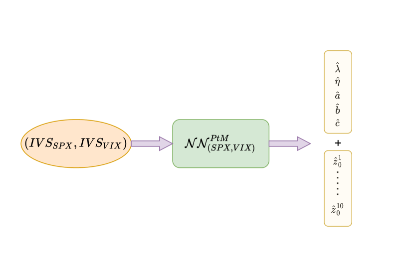
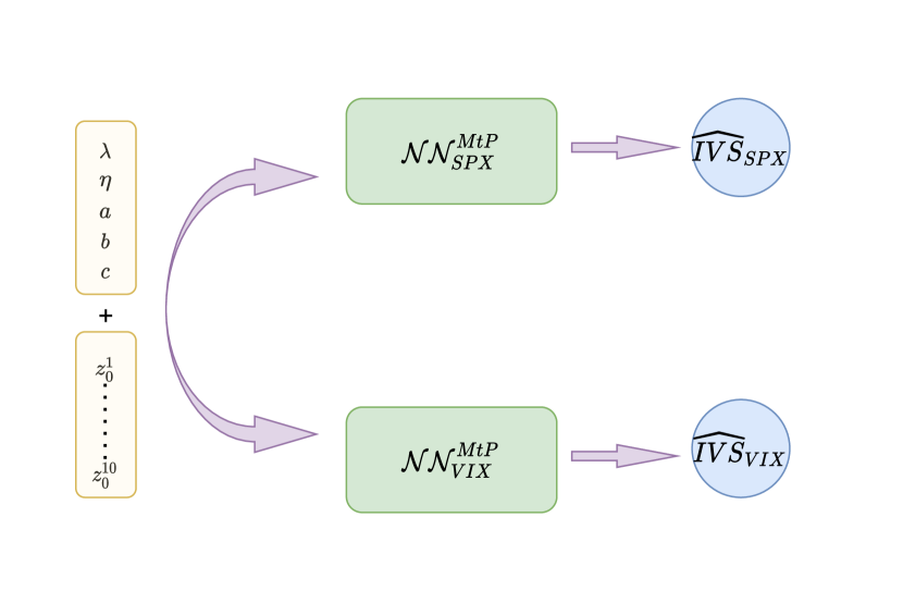
Figure 3.1: Scheme of PtM and MtP method.

We denote the neural network of PtM method by $\mathcal{NN}^{PtM}_{(SPX,VIX)}:\text{R}_{+}^{2m}\mapsto\Omega\times\mathcal{Z}$. It takes $IVS_{SPX}$ and $IVS_{VIX}$ as input, and outputs estimation of parameters $\boldsymbol{\omega}$ and $\mathbf{z}_{0}$. As for MtP method, the network consists of two sub-networks, denoted with $\mathcal{NN}^{MtP}_{SPX}:\Omega\times\mathcal{Z}\mapsto\text{R}_{+}^{m}$ and $\mathcal{NN}^{MtP}_{VIX}:\Omega\times\mathcal{Z}\mapsto\text{R}_{+}^{m}$. They aim at approximating the mappings from model parameters to $IVS_{SPX}$ and $IVS_{VIX}$ respectively. The methodology is illustrated in Figure 3.1. Table 3.1 summarizes some key characteristics of these networks and the training process. Note that for model training, each element of $\boldsymbol{\omega}$ and $\mathbf{z}_{0}$ is standardized to be in $[-1,1]$, every point of the $IVS^{MC}$ is subtracted by the sample mean, and divided by the sample standard deviation across training set.

	$\mathcal{NN}^{PtM}_{(SPX,VIX)}$	$\mathcal{NN}^{MtP}_{SPX}$	$\mathcal{NN}^{MtP}_{VIX}$
Input dimension	120	15	15
Output dimension	15	60	60
Hidden layers	7 with 25 hidden nodes for each, followed by SiLU activation function, see [18]
Training epochs	150 epochs with early stopping if not improved on validation set for 5 epochs
Others	Adam optimizer, initial learning rate 0.001, reduced by a factor of 2 every 10 epochs, mini-batch size 128

Table 3.1: Some key characteristics of the networks and the training process.

3.2 Pricing

Figure 3.2: Average Monte-Carlo absolute errors of implied volatilities across test set, defined as the half 95% confidence interval of Monte-Carlo simulations.

In this part we first check the ability of neural networks to approximate the pricing function of the model, i.e. the mapping from model parameters to $IVS_{SPX}$ and $IVS_{VIX}$. To see this, we compare the estimations $\widehat{IVS}_{SPX}$ and $\widehat{IVS}_{VIX}$, given by $\mathcal{NN}_{SPX}^{MtP}$ and $\mathcal{NN}_{VIX}^{MtP}$, with the “true” counterparts given by Monte-Carlo method.

Figure 3.2 presents the benchmark, given by the half 95% confidence interval of Monte-Carlo simulations for each points on $IVS_{SPX}$ and $IVS_{VIX}$. We then apply $\mathcal{NN}^{MtP}_{SPX}$ and $\mathcal{NN}^{MtP}_{VIX}$ on test set and evaluate the average absolute errors $\big{(}\text{abs}(\widehat{IVS}_{I}-IVS_{I}^{MC})\big{)}_{I=SPX,VIX}$. The results are shown in Figure 3.3. We can see that the estimations given by neural networks are close to Monte-Carlo references, with the majority of points of IVS falling in the 95% confidence interval of Monte-Carlo. We also tested average relative errors as an alternative metric, defined as $\big{(}\text{abs}(\widehat{IVS}_{I}-IVS_{I}^{MC})\oslash IVS_{I}^{MC}\big{)}_{I=SPX,VIX}$, where $\oslash$ means element-wise division between vectors. The results are given in Figure C.1 and Figure C.2 in Appendix, and are consistent with the observations in Figures 3.2-3.3.

Figure 3.3: Average absolute errors of implied volatilities across test set for $\mathcal{NN}^{MtP}_{SPX}$ and $\mathcal{NN}^{MtP}_{VIX}$. Errors are calculated with respect to Monte-Carlo counterparts.

At this stage, it is reasonable to conclude that $\mathcal{NN}^{MtP}_{SPX}$ and $\mathcal{NN}^{MtP}_{VIX}$ are able to learn the pricing functions from data of Monte-Carlo simulations. With these networks we can generate implied volatility surfaces for SPX and VIX for any model parameters.

3.3 Calibration

In this part, we use $\mathcal{NN}^{PtM}_{(SPX,VIX)}$, $\mathcal{NN}^{MtP}_{SPX}$ and $\mathcal{NN}^{MtP}_{VIX}$ to perform model calibration. For PtM method, the output of network gives directly calibration results. For MtP method, the result is given as

$$\hat{\boldsymbol{\omega}},\hat{\mathbf{z}}_{0}=\text{argmin}_{\boldsymbol{\omega}\in\Omega,\mathbf{z}_{0}\in\mathcal{Z}}\,\|\mathcal{NN}^{MtP}_{SPX}(\boldsymbol{\omega},\mathbf{z}_{0})-IVS_{SPX}\|^{2}_{2}+\|\mathcal{NN}^{MtP}_{VIX}(\boldsymbol{\omega},\mathbf{z}_{0})-IVS_{VIX}\|^{2}_{2}\,.$$ (3.1)

where $\Omega=[0.5,2.5]\times[1.0,1.5]\times[0.1,0.6]\times[0.01,0.5]\times[0.0001,0.03]$, $\mathcal{Z}=[-0.5,0.5]^{10}$. We use the same weight for all points of IVS in (3.1). In practice we could consider different weights to adapt to the varying nature of market quotes in terms of liquidity, bid-ask spread, etc. We apply L-BFGS-B algorithm for this optimization problem. Note that it is a gradient-based algorithm, and the gradients needed are calculated directly with $\mathcal{NN}_{SPX}^{MtP}$ and $\mathcal{NN}_{VIX}^{MtP}$ via automatic adjoint differentiation (AAD), which is already implemented in popular deep learning frameworks like TensorFlow and PyTorch. One can refer to Section 4.1 for calculation principles.

Calibration on simulated data

We apply the two methods on test set generated by Monte-Carlo simulations, and we evaluate the calibration by Normalized Absolute Errors (NAE) of parameters and the reconstruction Root Mean Square Errors (RMSE) of IVS:

NAE $$=\frac{|\hat{\theta}-\theta|}{\theta_{up}-\theta_{low}}\,,$$

RMSE $$=\sqrt{\frac{1}{\#k_{I}\times\#T}\|\mathcal{NN}^{MtP}_{I}(\hat{\boldsymbol{\omega}},\mathbf{\hat{z}}_{0})-IVS^{MC}_{I}\|_{2}^{2}},\quad I\in\{\text{SPX},\text{VIX}\}\,,$$

where $\theta$ is one element of $\boldsymbol{\omega}$ or $\mathbf{z}_{0}$, and $\theta_{up},\theta_{low}$ stand for the upper bound and lower bound of the uniform distribution for sampling $\theta$. Note that we could alternatively use Monte-Carlo to reconstruct IVS with the calibrated parameters instead of $\mathcal{NN}^{MtP}_{SPX}$ and $\mathcal{NN}^{MtP}_{VIX}$. However it would be much slower and we have seen in the above that the outputs given by $\mathcal{NN}^{MtP}_{SPX}$ and $\mathcal{NN}^{MtP}_{VIX}$ are very close to those of Monte-Carlo. Figure C.3 in Appendix shows the empirical cumulative distribution function of NAE for all the calibrated parameters. Figure 3.4 gives the empirical distribution of RMSE of IVS with the calibrated parameters from the two methods. We can make the following remarks:

• From Figure C.3 in Appendix, we see that PtM method can usually get smaller discrepancy for calibrated parameters than MtP method. This is not surprising since the latter may end with locally optimal solutions when we use gradient-based optimization algorithms.

• MtP method performs better in terms of reconstruction error, which is expected since it is exactly what the algorithm tries to minimize.

• Our results are of course not as accurate as those reported in [20] for some other rough volatility models, especially in terms of calibration errors for model parameters. This is because our model is more complex and has more parameters. Consequently more data and more complicated network architecture are demanded for training. The algorithms are also more likely to end with locally optimal solutions.

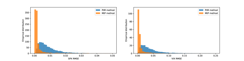
Figure 3.4: Empirical distribution of reconstruction RMSE of IVS.

Calibration on market data

We use MtP approach on market data since there are no “true” reference model parameter values in this case, and the objective is to minimize the discrepancy between model outputs and market observations. The arbitrage-free implied volatility interpolation method presented in [12] is used to generate IVS with the same log-moneyness strikes and maturities as before. Taking the data of 19 May 2017 tested in [14] as example, we get the following calibration results:

$$\boldsymbol{\omega} =(2.5,1.485,0.401,0.235,0.001),$$

$$\mathbf{z}_{0} =(-0.033,0.015,-0.004,0.017,0.028,0.098,0.192,-0.076,0.072,-0.062)\,.$$

We then use Monte-Carlo to get whole IVS of SPX and VIX with these parameters. The slices corresponding to several existing maturities in the market are shown in Figure 3.5 and Figure 3.6.

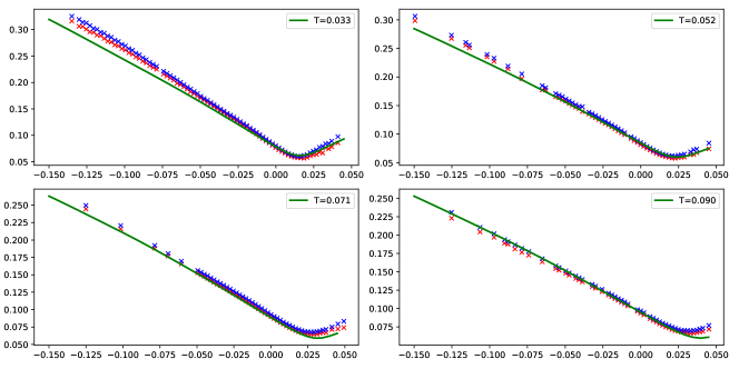
Figure 3.5: Implied volatilities on SPX options for 19 May 2017. Bid and ask of market volatilities are represented respectively by red and blue points. Green line is the output of model with Monte-Carlo method.

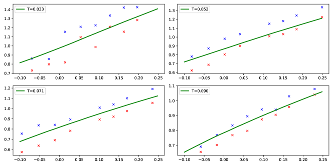
Figure 3.6: Implied volatilities on VIX options for 19 May 2017. Bid and ask of market volatilities are represented respectively by red and blue points. Green line is the output of model with Monte-Carlo method.

Our model fits very well the globe shape of IVS of SPX and VIX options at the same time. Model’s outputs fall essentially between bid and ask quotes for VIX options. In addition, excellent fits are obtained in terms of at-the-money skew of SPX options . Note that we do not require the market quotes of SPX options and VIX options to have same maturities. Another example of joint calibration is given in Appendix C.2.

Figure C.6 in Appendix presents the historical dynamics of parameters from daily calibration on market data. It is interesting to remark that during the beginning of COVID-19 crisis, $a,b,c$ all increased, which means stronger feedback effect, more distinct feedback asymmetry and larger base variance level. The quantity $Z_{0}:=\sum_{i=1}^{10}c_{i}z^{i}_{0}$ became negative. All these changes contributed to larger volatility.

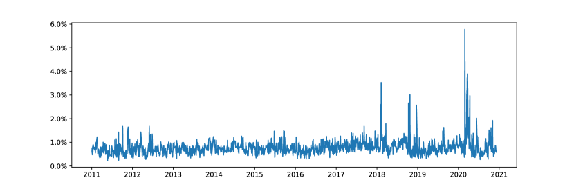
Figure 3.7: Historical reconstruction RMSE of $IVS_{SPX}$.

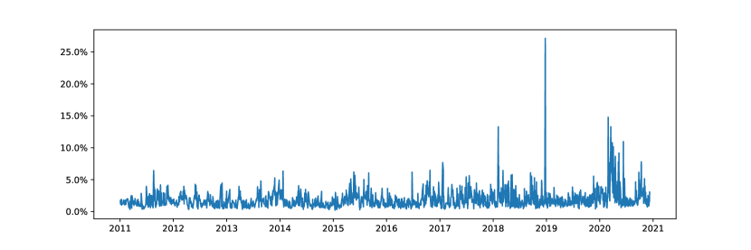
Figure 3.8: Historical reconstruction RMSE of $IVS_{VIX}$.

Figures 3.7 and 3.8 show historical RMSE for $IVS_{SPX}$ and $IVS_{VIX}$. For most time periods, the model can fit very well the two IVS at the same time, with small RMSE. For certain dates with extremely large market moves, we observe some spikes of errors. In fact for these dates market liquidity is usually very concentrated on one type of contract (Call or Put) with specific strikes and maturities. In this case, market IVS is not smooth enough so that the model may fail to output satisfying fit. Alternative more robust IVS interpolation methods could be tested in practice to generate smoother IVS. We could also focus only on some points of interest on IVS by excluding other points from the calibration objective (3.1). Note that all the empirical results presented here are with $\alpha=0.51$ and $n=10$. Interested readers can try other $\alpha$ or bigger $n$ to improve globally historical RMSE, while new synthetic data need to be generated for each new setting.

4 Toy examples for hedging

We have seen in the previous section that the proposed model can jointly fit $IVS_{SPX}$ and $IVS_{VIX}$ with small errors. Then it is important to know how to hedge options with this model. In this section, we give toy examples on synthetic data and market data as well to show how to use the neural networks to perform hedging for vanilla SPX calls. We will see that in our model perfect hedging for these products is possible with only SPX.

4.1 Hedging portfolio computation with neural networks

Let $\mathbf{Z}_{t}:=(Z^{1}_{t},\cdots,Z^{10}_{t})$ and $\mathbf{X}_{t}:=(S_{t},\mathbf{Z}_{t})$. As indicated in Remark (2.1), Model (2.3-2.5) being Markovian, given strike $K$, maturity $T$ and model parameters $\boldsymbol{\omega}$, the price of vanilla SPX call at time $t$ is then a function of $\mathbf{X}_{t}$. Let $P_{t}(\mathbf{X}_{t};K,T,\boldsymbol{\omega})$ denote this quantity. With the dynamics of $(Z^{i}_{t})_{i=1,\cdots,10}$ in Equation (2.5), we then have

$$dP_{t}(\mathbf{X}_{t};K,T,\boldsymbol{\omega})=\delta_{t}dS_{t}\,,$$ (4.1)

where

$$\delta_{t}=\frac{\partial P_{t}(\mathbf{X}_{t};K,T,\boldsymbol{\omega})}{\partial S_{t}}+\frac{\eta}{S_{t}}\sum_{i=1}^{10}\frac{\partial P_{t}(\mathbf{X}_{t};K,T,\boldsymbol{\omega})}{\partial Z^{i}_{t}}\,.$$ (4.2)

Note that the factors $(Z^{i})_{i=1,\cdots,10}$ can be fully traced because they are assumed to be driven by the same Brownian motion as $S$, which is observable from market data. With the neural networks approximating the pricing function of the model, we will see that we can then obtain approximation of $\delta_{t}$ for any $t$. Of course continuous hedging is impossible in practice. Here we perform discrete hedging with time step $\Delta t$. The Profit and Loss (P&L) of hedging at $t\in(0,T]$ is given by

$$\mathcal{J}_{t}=\mathcal{J}^{\delta}_{t}-\mathcal{J}^{P}_{t},$$ (4.3)

where

$$\mathcal{J}^{\delta}_{t} =\sum_{k=0}^{\left\lfloor t/\Delta t\right\rfloor-1}\hat{\delta}_{t_{k}}\triangle S_{t_{k+1}}+\hat{\delta}_{t_{\left\lfloor t/\Delta t\right\rfloor}}(S_{t}-S_{\left\lfloor t/\Delta t\right\rfloor\Delta t})\,,$$

$$\mathcal{J}^{P}_{t} =P_{t}-P_{0}\,,$$

with $t_{k}=k\triangle t$, $\triangle S_{t_{k}}:=S_{t_{k}}-S_{t_{k-1}}$, $\hat{\delta}_{t_{k}}$ is the hedging ratio given by neural networks at $k$-th hedging time $t_{k}$, and $P_{t}$ is the price of the SPX option to hedge at time $t$. As we can see, $\mathcal{J}^{\delta}$ stands for the P&L coming from holding the underlying and $\mathcal{J}^{P}$ reflects the price evolution of the option. We show in the following that $\hat{\delta}_{t_{k}}$ can be given directly from $\mathcal{NN}_{SPX}^{MtP}$ in our model.

Note that $\mathcal{NN}_{SPX}^{MtP}$ behaves like a “global” pricer that is reusable under any model parameters $\boldsymbol{\omega}$. Given $\boldsymbol{\omega}$, we could actually train a finer network as a “local” pricer taking only $\mathbf{z}_{0}$ as input. Of course the same methodology as before can be used with fixed $\boldsymbol{\omega}$. Here we apply alternatively Differential Machine Learning as a fast method to obtain approximation of pricing function from simulated paths, under a given calibration of the model, see [21].

Method 1: with $\mathcal{NN}_{SPX}^{MtP}$

With $\mathcal{NN}_{SPX}^{MtP}$ outputing implied volatilities with respect to log-moneyness strikes, we have

$$P_{t}(\mathbf{X}_{t};K,T,\boldsymbol{\omega})\simeq P^{BS}\big{(}S_{t},K,T-t,\sigma_{\mathcal{NN}}^{\log(K/S_{t}),T-t}(\boldsymbol{\omega},\mathbf{Z}_{t})\big{)}\,,$$

where $P^{BS}(S,K,T,\sigma)$ is the price of European call under Black-Scholes model and $\sigma_{\mathcal{NN}}^{k,T}(\boldsymbol{\omega},\mathbf{Z}_{t})$ is the implied volatility corresponding to log-moneyness strike $k$ and maturity $T$, calculated directly by $\mathcal{NN}^{MtP}_{SPX}$ with $(\boldsymbol{\omega},\mathbf{Z}_{t})$ as input. Then the partial derivatives in (4.2) are given by

$$\begin{split}\frac{\partial P_{t}(\mathbf{X}_{t};K,T,\boldsymbol{\omega})}{\partial S_{t}}&\simeq\delta_{BS}\big{(}S_{t},K,T-t,\sigma_{\mathcal{NN}}^{\log(K/S_{t}),T-t}(\boldsymbol{\omega},\mathbf{Z}_{t})\big{)}+\\ &\nu_{BS}\big{(}S_{t},K,T-t,\sigma_{\mathcal{NN}}^{\log(K/S_{t}),T-t}(\boldsymbol{\omega},\mathbf{Z}_{t})\big{)}\frac{\partial\sigma_{\mathcal{NN}}^{k,T-t}(\boldsymbol{\omega},\mathbf{Z}_{t})}{\partial k}\lvert_{k=\log(K/S_{t})}\frac{\partial\log(K/S_{t})}{\partial S_{t}},\,\end{split}$$ (4.4)

$$\frac{\partial P_{t}(\mathbf{X}_{t};K,T,\boldsymbol{\omega})}{\partial Z_{t}^{i}}\simeq\nu_{BS}\big{(}S_{t},K,T-t,\sigma_{\mathcal{NN}}^{\log(K/S_{t}),T-t}(\boldsymbol{\omega},\mathbf{Z}_{t})\big{)}\frac{\partial\sigma_{\mathcal{NN}}^{\log(K/S_{t}),T-t}(\boldsymbol{\omega},\mathbf{Z}_{t})}{\partial Z^{i}_{t}},\,$$ (4.5)

where $\delta_{BS}(S,K,T,\sigma)$ and $\nu(S,K,T,\sigma)$ stand for the Delta and Vega respectively under Black-Scholes model. The quantity $\frac{\partial\sigma_{\mathcal{NN}}^{k,T}}{\partial Z^{i}_{t}}$ corresponds actually to the derivative of the outputs of $\mathcal{NN}^{MtP}_{SPX}$ with respect to its inputs. Thus it can be obtained instantaneously with built-in AAD. $\frac{\partial\sigma_{\mathcal{NN}}^{k,T-t}(\boldsymbol{\omega},\mathbf{Z}_{t})}{\partial k}$ in (4.4) can be approximated by the finite difference $\frac{(\sigma^{k+\delta_{k},T-t}_{\mathcal{NN}}-\sigma^{k-\delta_{k},T-t}_{\mathcal{NN}})}{2\delta_{k}}(\boldsymbol{\omega},\mathbf{Z}_{t})$. Note that some interpolation methods need to be applied for arbitrary pair $(K,T-t)$ since $\mathcal{NN}^{MtP}_{SPX}$ has fixed log-moneyness strikes and maturities.

Method 2: with Differential Machine Learning

Given parameters $\boldsymbol{\omega}$, we can simulate a path of model state $(\mathbf{X}_{t})_{0\leq t\leq T}$ starting from the initial state $\mathbf{X}_{0}$. The pathwise payoff $(S_{T}-K)_{+}$ is in fact an unbiased estimation of $P_{0}(\mathbf{X}_{0};K,T,\boldsymbol{\omega})$. Under some regularity conditions, the pathwise derivative $\frac{\partial(S_{T}-K)_{+}}{\partial\mathbf{X}_{0}}$ is also an unbiased estimation of $\frac{\partial P_{0}(\mathbf{X}_{0};K,T,\boldsymbol{\omega})}{\partial\mathbf{X}_{0}}$. We show in the following how to calculate this quantity with the simulation scheme proposed in (A.1). The basic idea of Differential Machine Learning [15, 21] is to concatenate pathwise payoff and pathwise derivatives as targets to train a neural network, denoted by $\mathcal{NN}_{DML}$, to approximate the pricing mapping from $\mathbf{X}_{0}$ to $P_{0}$ under some fixed $\boldsymbol{\omega}$. Thus, the training samples are like $\big{\{}\mathbf{X}_{0},\big{(}(S_{T}-K)_{+},\frac{\partial(S_{T}-K)_{+}}{\partial\mathbf{X}_{0}}\big{)}\big{\}}$, and the loss function for training is like

$$\mathcal{L}=\mathcal{L}_{1}\big{(}\mathcal{NN}_{DML}(\mathbf{X}_{0}),(S_{T}-K)_{+}\big{)}+\mathcal{L}_{2}\big{(}\frac{\partial\mathcal{NN}_{DML}(\mathbf{X}_{0})}{\partial\mathbf{X}_{0}},\frac{\partial(S_{T}-K)_{+}}{\partial\mathbf{X}_{0}}\big{)}\,,$$ (4.6)

with $\mathcal{L}_{1}$ and $\mathcal{L}_{2}$ some suitably chosen loss functions. Similarly to the case with $\mathcal{NN}^{MtP}_{SPX}$, $\frac{\partial\mathcal{NN}_{DML}(\mathbf{X}_{0})}{\partial\mathbf{X}_{0}}$ can be calculated efficiently with AAD. In this way, $\mathcal{NN}_{DML}$ aims at learning both the pricing function and its derivatives during training. This can help the networks converge with few samples, see [21].

The quantity $\frac{\partial(S_{T}-K)_{+}}{\partial\mathbf{X}_{0}}$ can be calculated with AAD, which is based on the chain rule of derivatives computation, see [15] for more details. In our case, with the Euler scheme in (A.1), let $\Delta t$ the simulation step with $N\Delta t=T$. We have

$$\frac{\partial\hat{S}_{k+1}}{\partial X^{j}_{0}} =\big{(}1+\sqrt{\hat{V}_{k}}(W_{k+1}-W_{k})\big{)}\frac{\partial\hat{S}_{k}}{\partial X^{j}_{0}}+\frac{a\hat{S}_{k}(W_{k+1}-W_{k})(\sum_{i=1}^{10}c_{i}\hat{Z}^{i}_{k}-b)}{\sqrt{\hat{V}_{k}}}\sum_{i=1}^{10}c_{i}\frac{\partial\hat{Z}^{i}_{k}}{\partial X^{j}_{0}}\,,$$

$$\frac{\partial\hat{Z}^{i}_{k+1}}{\partial X^{j}_{0}} =\frac{1}{1+\gamma_{i}\Delta t}\big{(}\frac{\partial\hat{Z}^{i}_{k}}{\partial X^{j}_{0}}+(-\lambda\Delta t+\frac{\eta a(W_{k+1}-W_{k})(\sum_{i=1}^{10}c_{i}\hat{Z}^{i}_{k}-b)}{\sqrt{\hat{V}_{k}}})\sum_{i=1}^{10}c_{i}\frac{\partial\hat{Z}^{i}_{k}}{\partial X^{j}_{0}}\big{)}\,,$$

where $X^{j}_{0}$ is the $j$-th element of $\mathbf{X}_{0}$. Let $\mathbf{\hat{X}}_{k}:=(\hat{S}_{k},\hat{Z}^{1}_{k},\cdots,\hat{Z}^{10}_{k})$. This can be rewritten in matrix form $\boldsymbol{\Delta}(k+1)=\mathbf{D}(k)\mathbf{\Delta}(k)$, with $\mathbf{\Delta}_{i,j}(k)=\frac{\partial\hat{X}^{i}_{k}}{\partial X^{j}_{0}},i,j=1,\cdots,11$, and

$$\mathbf{D}(k)=\begin{pmatrix}1+\sqrt{\hat{V}_{k}}\Delta W_{k+1},&\hat{S}_{k}M^{1}_{k}c_{1},&\cdots&\hat{S}_{k}M^{1}_{k}c_{10}\\ 0,&\frac{1+c_{1}M^{2}_{k}}{1+\gamma_{1}\Delta t},&\cdots&\frac{c_{10}M^{2}_{k}}{1+\gamma_{10}\Delta t}\\ \vdots&\vdots&\vdots&\vdots\\ 0&\frac{c_{1}M_{k}^{2}}{1+\gamma_{1}\Delta t},&\cdots&\frac{1+c_{10}M_{k}^{2}}{1+\gamma_{10}\Delta t}\end{pmatrix}\,,$$

where

$$\Delta W_{k+1} :=W_{k+1}-W_{k}\,,$$

$$M_{k}^{1} :=\frac{a\Delta W_{k+1}(\sum_{i=1}^{10}c_{i}\hat{Z}_{k}^{i}-b)}{\sqrt{\hat{V}_{k}}}\,,$$

$$M_{k}^{2} :=\eta M^{1}_{k}-\lambda\Delta t\,.$$

Then we have

$$\begin{split}\frac{\partial(\hat{S}_{T}-K)_{+}}{\partial\mathbf{X}_{0}}&=\mathbf{\Delta}(N)^{T}\frac{\partial(\hat{S}_{T}-K)_{+}}{\partial\mathbf{\hat{X}}_{N}}\\ &=\mathbf{\Delta}(0)^{T}\mathbf{D}(0)^{T}\cdots\mathbf{D}(N-2)^{T}\mathbf{D}(N-1)^{T}\frac{\partial(\hat{S}_{T}-K)_{+}}{\partial\mathbf{\hat{X}}_{N}}\\ &=\mathbf{\Delta}(0)^{T}\mathbf{V}(0)\,,\end{split}$$ (4.7)

where $\mathbf{\Delta}(0)$ is simply the identity matrix by definition, and $\mathbf{V}(0)$ can be calculated recursively:

$$\begin{split}\mathbf{V}(k)&=\mathbf{D}(k)^{T}\mathbf{V}(k+1),\quad k=0,\cdots,N-1\,,\\ \mathbf{V}(N)&=\frac{\partial(\hat{S}_{T}-K)_{+}}{\partial\mathbf{\hat{X}}_{N}}=\mathbf{1}(\hat{S}_{T}>K)(1,0,\cdots,0)^{T}\,.\end{split}$$ (4.8)

Note that for each simulated path, $\big{(}\mathbf{D}(k)\big{)}_{k=0,\cdots,N-1}$ can be readily obtained, so the quantity $\frac{\partial(\hat{S}_{T}-K)_{+}}{\partial\mathbf{X}_{0}}$ can be efficiently computed following (4.7, 4.8).

Since we use the same trained network for hedging at any $t\in(0,T]$, to accommodate the varying time to maturity $(T-t)$, we consider multiple outputs corresponding to different maturities ${T_{1},T_{2},\cdots,T_{m}}$ for $\mathcal{NN}_{DML}$, with $T_{1}<T<T_{m}$. The quantities $(\frac{\partial(\hat{S}_{T_{i}}-K)_{+}}{\partial\mathbf{X}_{0}})_{i=1,\cdots,m}$ can be computed following (4.7, 4.8). For training, we use the average of $m$ derivatives in (4.6) for simplification, see [21] for more details on designs with multi-dimensional output. After training $\mathcal{NN}_{DML}$ with respect to strike $K$ and parameter $\boldsymbol{\omega}$, we have

$$P_{t}(\mathbf{X}_{t};K,T,\boldsymbol{\omega})\simeq\mathcal{NN}_{DML}^{T-t}(\mathbf{X}_{t})\,,$$

with $\mathcal{NN}_{DML}^{T-t}(\cdot)$ the output corresponding to maturity $(T-t)$. Thus we get

$$\frac{\partial P_{t}(\mathbf{X}_{t};K,T,\boldsymbol{\omega})}{\partial S_{t}} \simeq\frac{\partial\mathcal{NN}_{DML}^{T-t}(\mathbf{X}_{t})}{\partial S_{t}}\,,$$

$$\frac{\partial P_{t}(\mathbf{X}_{t};K,T,\boldsymbol{\omega})}{\partial Z_{t}^{i}} \simeq\frac{\partial\mathcal{NN}_{DML}^{T-t}(\mathbf{X}_{t})}{\partial Z_{t}^{i}}\,.$$

Then the formula in (4.2) is used to obtain hedging ratio. As in the case with $\mathcal{NN}^{MtP}_{SPX}$, some interpolation methods are needed for arbitrary $(T-t)$. In our tests, we choose the following characteristics for $\mathcal{NN}_{DML}$ and its training:

• 4 hidden layers, with 20 hidden nodes for each, SiLU as activation function,

• input dimension is 11, output dimension is 5 corresponding to maturities $0.02,0.04,0.06,0.08,0.1$,

• mini-batch gradient descent with batch size 128, initial learning rate 0.001, divided by 2 every 5 epochs,

• sample uniformly $\mathbf{X}_{0}$ and simulate 50,000 paths, train $\mathcal{NN}_{DML}$ with 20 epochs.

4.2 Numerical results

Hedging on synthetic data

Without loss of generality, we take the following parameters in the experiments:

• $\boldsymbol{\omega}=(1,1.2,0.35,0.2,0.0025)$

• $S_{0}=100,Z^{i}_{0}=0,i=1,\cdots,10$

• $K=98,T=0.08$

First we generate 50,000 paths of $(S_{t})_{0\leq t\leq T}$ by following the scheme A.1 with time step $\Delta t=0.0012$. The price $P_{0}$ is estimated by the average of pathwise payoffs. Then we evaluate $\mathcal{J}_{T}$ for 5000 paths among them, with hedging time step $\Delta t\in\{0.0012,0.0036\}$. From Figure 4.1 we can see that both methods lead to hedging payoffs around 0. Hedging less frequently brings slightly larger variance of payoffs. We also remark that the method with $\mathcal{NN}^{MtP}_{SPX}$ generates smaller variance than the other with $\mathcal{NN}_{DML}$. It is expected as the latter is trained with pathwise labels while the former is trained with “true” labels given by Monte-Carlo means, which have certainly smaller variance.

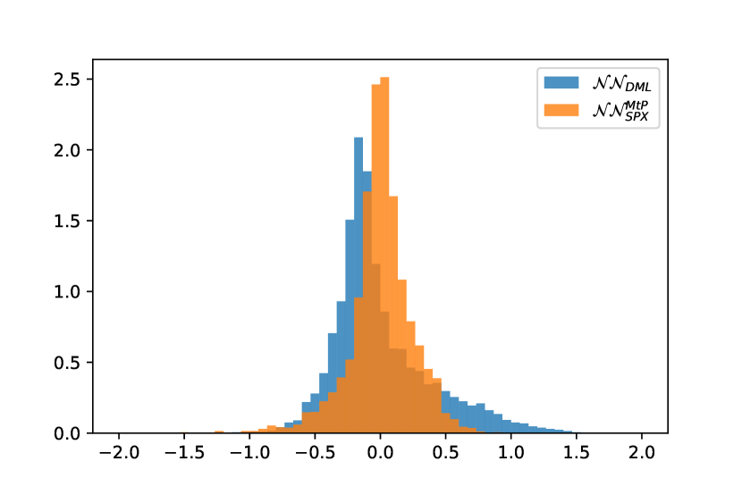
(a) $\Delta_{t}=0.0012$ (three times daily)

(b) $\Delta_{t}=0.0036$(daily)

Figure 4.1: Hedging P&L with $\mathcal{NN}_{DML}$ and $\mathcal{NN}_{SPX}^{MtP}$ on simulated data. $P_{0}$ given by Monte-Carlo is 2.9.

Hedging on market data

We perform daily hedging on two SPX monthly calls:

1. Maturity date 16 June 2017, strike 2425, hedged since 18 May 2017.

2. Maturity date 16 February 2018, strike 2750, hedged since 18 January 2018.

Figure 4.2: Hedging P&L on two SPX calls with maturity 16 June 2017, strike 2425 (left), and maturity 16 February 2018, strike 2750 (right).

On first day of hedging, we take market data for model calibration and get $\boldsymbol{\omega}$ and $\mathbf{z}_{0}$. $\mathcal{NN}_{DML}$ is then trained on paths generated under $\boldsymbol{\omega}$. Then for each following day, we update the value of factors $(Z^{i})_{i=1,\cdots,10}$ with respect to the evolution of SPX, and we compute the hedging portfolio with $\mathcal{NN}_{SPX}^{MtP}$ and $\mathcal{NN}_{DML}$ as explained in the above. Besides, we also test with Black-Scholes model where the implied volatility of the first day is used to compute Delta as hedging ratio. Figure 4.2 presents the evolution of $\mathcal{J}^{P}$ and $\mathcal{J}^{\delta}$ for these two examples. Note that all quantities are divided by $P_{0}$ to be unitless. We see that $\mathcal{NN}_{SPX}^{MtP}$ and $\mathcal{NN}_{DML}$ can follow very well the market price of options, with smaller $|\mathcal{J}_{T}|$ than Black-Scholes approach. Of course, in practice we need to consider more elements like hedging cost, slippage, and to do more tests for systematic comparison, but this is out of the scope of our current work.

5 Conclusion

We have seen that the deep neural networks can be used in calibrating the quadratic rough Heston model with reliable results. The training of network demands indeed lots of simulated data, especially when the dimension of model parameters is high. However, it is done off-line only once and the network will be reusable in many situations. Under the particular setting of our model, we can also use the network for risk hedging. Certainly, we can still improve the results presented in the above, for example fixing finer grids of strikes and maturities, or using more factors for the approximation. We emphasize that the methodologies presented in our work are of course not limited to the model introduced here, and can be adapted to other models and other financial products.

Appendix A Kernel function approximation and simulation scheme

Here we recall the geometric partition of $(c^{n}_{i},\gamma^{n}_{i})_{i=1,\cdots,n}$ proposed in [1]:

$$c^{n}_{i}=\int_{\eta^{n}_{i-1}}^{\eta^{n}_{i}}\mu(dx),\quad\gamma^{n}_{i}=\frac{1}{c^{n}_{i}}\int_{\eta^{n}_{i-1}}^{\eta^{n}_{i}}x\mu(dx),\quad i=1,\cdots,n\,,$$

with $\mu(dx)=\frac{x^{-\alpha}}{\Gamma(\alpha)\Gamma(1-\alpha)}dx$ and $\eta^{n}_{i}=x^{i-n/2}_{n}$. Hence we have

$$c^{n}_{i}=\frac{x_{n}^{(1-\alpha)(i-n/2)}(1-x_{n}^{\alpha-1})}{(1-\alpha)\Gamma(\alpha)\Gamma(1-\alpha)},\quad\gamma^{n}_{i}=\frac{(1-\alpha)x_{n}^{i-1-n/2}(x_{n}^{2-\alpha}-1)}{(2-\alpha)(x_{n}^{1-\alpha}-1)}\,.$$

Given $n$, $\alpha$ and $T$, we can determine the “optimal” $x_{n}$ as

$$x^{*}_{n}(\alpha,T)=\arg\min_{x^{*}_{n}>1}\|K^{n}-K\|_{L^{2}(0,T)}\,.$$

We fix $T=0.1$ as we are more interested in short maturities and we get the optimal $x^{*}_{n}$ for different $n$ and $\alpha$ as shown in Figure A.1. It is consistent with the analysis in [1] that given $\alpha$, we need to increase $x_{n}$ to mimic roughness with less factors. Given $n$, $x^{*}_{n}$ does not change a lot with $\alpha$, which indicates that in practice we can actually fix $x^{*}_{n}$ independently of $\alpha$.

Figure A.1: $x^{*}_{n}$ for different n and $\alpha$.

Choosing a good $n$ is a trade-off between simulation efficiency and good approximation of rough volatility models. In our test, we take $n=10$ and $x_{10}^{*}=3.92$. On one hand, we can see from Figure A.2 that the approximation of $K^{10}$ to $K$ is not far away from other $K^{n}$ with larger $n$. On the other hand, it means a margin for improvement with larger $n$. Figure A.3 gives the resulting $c_{i}^{n}$ and $\gamma_{i}^{n}$. We see that the wide range of $\gamma$ contributes to the multi-timescales nature of volatility processes.

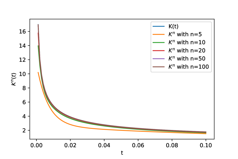
Figure A.2: $K(t)$ and $K^{n}(t)$ with different $n$ with $\alpha=0.51$.

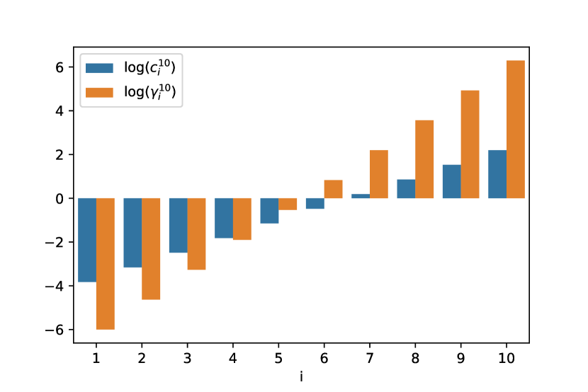
Figure A.3: Logarithm of $c_{i}^{10}$ and $\gamma_{i}^{10}$ by taking $x_{10}^{*}=3.92$.

We discard the notation $n$ and use the following modified explicit-implicit Euler scheme for simulating Model (2.3-2.5):

$$\begin{split}\hat{S}_{k+1}&=\hat{S}_{k}+\hat{S}_{k}\sqrt{\hat{V}_{k}}(W_{k+1}-W_{k}),\qquad\hat{V}_{k}=a(\hat{Z}_{k}-b)^{2}+c\,,\\ \hat{Z}^{i}_{k+1}&=\frac{1}{1+\gamma_{i}\Delta t}\big{(}\hat{Z}^{i}_{k}-\lambda\hat{Z}_{k}\Delta t+\eta\sqrt{\hat{V}_{k}}(W_{k+1}-W_{k})\big{)}\,,\\ \hat{Z}_{k}&=\sum_{i=1}^{n}c_{i}\hat{Z}^{i}_{k}\,,\end{split}$$ (A.1)

for a time step $\Delta t=T/N$, $k=1,\cdots,N$ and $(W_{k+1}-W_{k})\sim\mathcal{N}(0,\Delta t)$. One could also use the explicit sheme for $Z^{i}$ given by

$$\hat{Z}^{i}_{k+1}=(1-\gamma_{i}\Delta t)\hat{Z}^{i}_{k}-\lambda\hat{Z}_{k}\Delta t+\eta\sqrt{\hat{V}_{k}}(W_{k+1}-W_{k})\,.$$

However, with above $x_{10}^{*}$, we get $\gamma_{10}=542.32$. One then need $\Delta t$ to be necessarily small to ensure the scheme’s stability. Instead we could use

$$\hat{Z}^{i}_{k+1}-\hat{Z}^{i}_{k}=-\gamma_{i}\Delta t\hat{Z}^{i}_{k+1}-\lambda\hat{Z}_{k}\Delta t+\eta\sqrt{\hat{V}_{k}}(W_{k+1}-W_{k})\,,$$

which leads to Scheme A.1 and avoids this issue.

Appendix B Network training with transfer learning

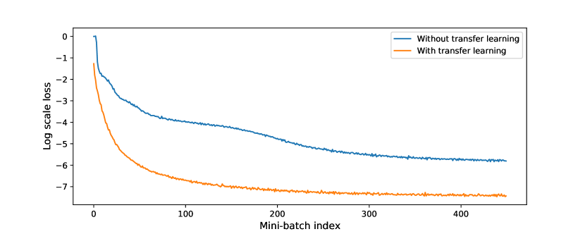
Figure B.1: Training loss evolution for $\alpha=0.65$ with 10,000 samples.

When we switch to models with $\alpha$ not equal to $0.51$, we can apply the idea of transfer learning to accelerate network training. More precisely, we use the parameters of the network corresponding to the case $\alpha=0.51$ to initialise the network for cases with different $\alpha$. Here we give an example on the training of $\mathcal{NN}_{SPX}^{MtP}$ with $\alpha=0.65$. With 10,000 training samples, we can see from Figure B.1 that transfer learning can help the training converge much faster to a lower loss than the one with random parameter initialization.

Appendix C Pricing and calibration with neural networks

C.1 On simulated data

Here we present the average relative pricing errors across test as an alternative evaluation metric. Figure C.1 stands for the benchmark given by Monte-Carlo and Figure C.2 gives the results with $\mathcal{NN}_{SPX}^{MtP}$ and $\mathcal{NN}_{VIX}^{MtP}$. Figure C.3 shows the accuracy of calibrated parameters by plotting the empirical CDFs of NAE.

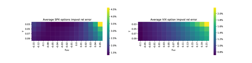
Figure C.1: Average Monte-Carlo relative errors of implied volatilities across test set, defined as the normalized half 95% confidence interval of Monte-Carlo simulations.

Figure C.2: Average relative errors of implied volatilities across test set for $\mathcal{NN}^{MtP}_{SPX}$ and $\mathcal{NN}^{MtP}_{VIX}$.

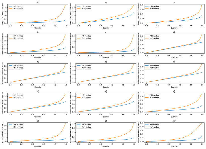
Figure C.3: Empirical CDF of NAE of calibrated parameters.

C.2 On market data

We give another IVS fit example on 10 September 2019. The parameters calibrated are:

$$\boldsymbol{\omega} =(1.717,1.5,0.265,0.246,0.0001)\,,$$

$$\mathbf{z}_{0} =(-0.009,0.015,0.011,0.036,0.002,-0.011,-0.018,0.074,0.142,-0.171)\,.$$

The Monte-Carlo results with these parameters are shown in Figure C.4 and Figure C.5. Figure C.6 presents the historical dynamics of parameters from daily calibration on market data.

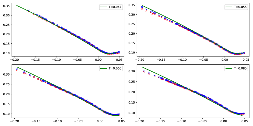
Figure C.4: Implied volatilities fit on SPX options for 10 September 2019. Bid and ask of market volatilities are represented respectively by red and blue points. Green line is the output of model with Monte-Carlo method.

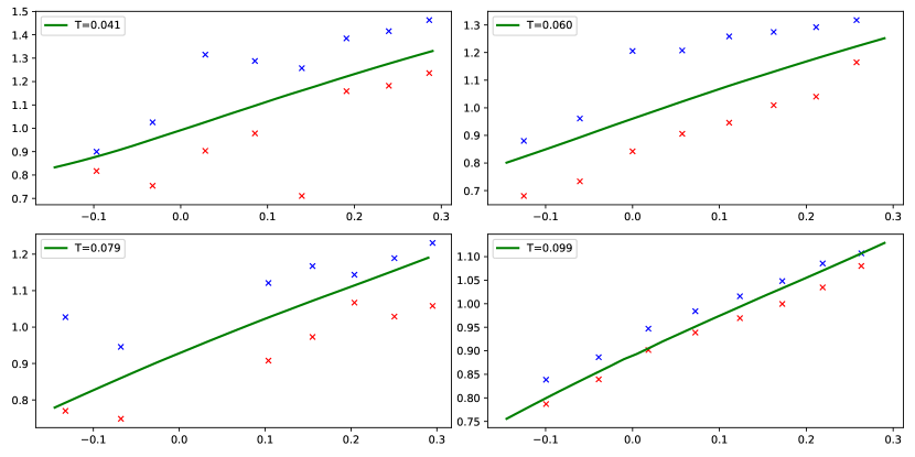
Figure C.5: Implied volatilities fit on VIX options for 10 September 2019. Bid and ask of market volatilities are represented respectively by red and blue points. Green line is the output of model with Monte-Carlo method.

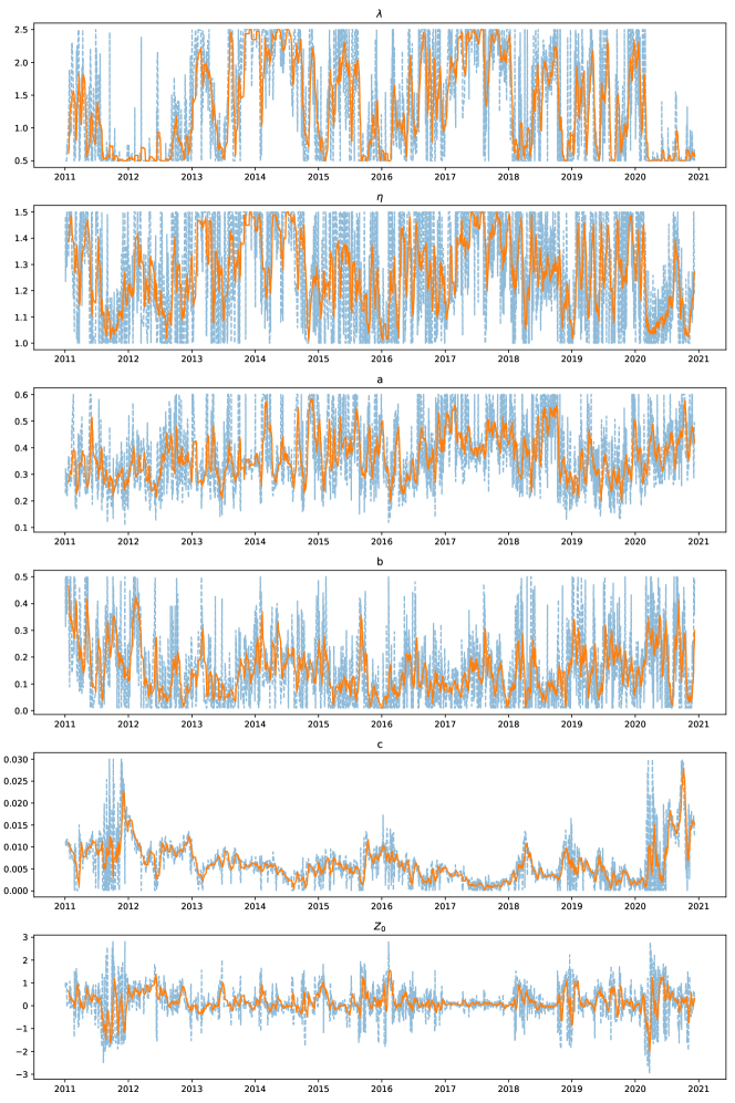
Figure C.6: Historical dynamics of calibrated parameters. The orange lines are 10-day moving average of parameters. Recall that $Z_{0}:=\sum_{i=1}^{10}c_{i}z^{i}_{0}$.

References

- [1] E. Abi Jaber. Lifting the Heston model. Quantitative Finance, 19(12):1995–2013, 2019.
- [2] E. Abi Jaber and O. El Euch. Multifactor approximation of rough volatility models. SIAM Journal on Financial Mathematics, 10(2):309–349, 2019.
- [3] C. Bayer, P. Friz, and J. Gatheral. Pricing under rough volatility. Quantitative Finance, 16(6):887–904, 2016.
- [4] C. Bayer, B. Horvath, A. Muguruza, B. Stemper, and M. Tomas. On deep calibration of (rough) stochastic volatility models. arXiv preprint arXiv:1908.08806, 2019.
- [5] M. Bennedsen, A. Lunde, and M. Pakkanen. Decoupling the short-and long-term behavior of stochastic volatility. Journal of Financial Econometrics, 2021.
- [6] A. Dandapani, P. Jusselin, and M. Rosenbaum. From quadratic Hawkes processes to super-Heston rough volatility models with Zumbach effect. Quantitative Finance, pages 1–13, 2021.
- [7] O. El Euch, M. Fukasawa, and M. Rosenbaum. The microstructural foundations of leverage effect and rough volatility. Finance and Stochastics, 22(2):241–280, 2018.
- [8] O. El Euch, J. Gatheral, and M. Rosenbaum. Roughening Heston. Risk, pages 84–89, 2019.
- [9] O. El Euch and M. Rosenbaum. Perfect hedging in rough Heston models. Annals of Applied Probability, 28(6):3813–3856, 2018.
- [10] O. El Euch and M. Rosenbaum. The characteristic function of rough Heston models. Mathematical Finance, 29(1):3–38, 2019.
- [11] J.-P. Fouque, G. Papanicolaou, R. Sircar, and K. Sølna. Multiscale stochastic volatility for equity, interest rate, and credit derivatives. Cambridge University Press, 2011.
- [12] J. Gatheral and A. Jacquier. Arbitrage-free SVI volatility surfaces. Quantitative Finance, 14(1):59–71, 2014.
- [13] J. Gatheral, T. Jaisson, and M. Rosenbaum. Volatility is rough. Quantitative Finance, 18(6):933–949, 2018.
- [14] J. Gatheral, P. Jusselin, and M. Rosenbaum. The quadratic rough Heston model and the joint S&P 500/VIX smile calibration problem. Risk, May, 2020.
- [15] M. Giles and P. Glasserman. Smoking Adjoints: fast Monte Carlo Greeks. Risk, 19(1):88–92, 2006.
- [16] I. Goodfellow, Y. Bengio, and A. Courville. Deep learning. MIT press, 2016.
- [17] J. Guyon. The joint S&P 500/VIX smile calibration puzzle solved. Risk, April, 2020.
- [18] D. Hendrycks and K. Gimpel. Gaussian error linear units (gelus). arXiv preprint arXiv:1606.08415, 2016.
- [19] A. Hernandez. Model calibration with neural networks. Available at SSRN 2812140, 2016.
- [20] B. Horvath, A. Muguruza, and M. Tomas. Deep learning volatility: a deep neural network perspective on pricing and calibration in (rough) volatility models. Quantitative Finance, 21(1):11–27, 2021.
- [21] B. N. Huge and A. Savine. Differential Machine Learning. Risk, October, 2020.
- [22] T. Jaisson and M. Rosenbaum. Rough fractional diffusions as scaling limits of nearly unstable heavy tailed Hawkes processes. Annals of Applied Probability, 26(5):2860–2882, 2016.
- [23] G. Livieri, S. Mouti, A. Pallavicini, and M. Rosenbaum. Rough volatility: evidence from option prices. IISE transactions, 50(9):767–776, 2018.
- [24] G. Zumbach. Volatility conditional on price trends. Quantitative Finance, 10(4):431–442, 2010.