Physical properties of the Hall current

Abstract

We study the stationary state of Hall devices composed of a load circuit connected to the lateral edges of a Hall-bar. We follow the approach developed in a previous work (Creff et al. J. Appl. Phys 2020) in which the stationary state of a ideal Hall bar is defined by the minimum power dissipation principle. The presence of both the lateral circuit and the magnetic field induces the injection of a current: the so-called Hall current. Analytical expressions for the longitudinal and the transverse currents are derived. It is shown that the efficiency of the power injection into the lateral circuit is quadratic in the Hall angle and obeys to the maximum transfer theorem. For usual values of the Hall angle, the main contribution of this power injection provides from the longitudinal current flowing along the edges, instead of the transverse current crossing the Hall bar.

I Introduction

The classical Hall effect Hall ; Corbino is usually described by the local transport equations for the charge carriers that takes into account the effect of the Laplace-Lorentz force generated by a static magnetic field. Typically, in a planar Hall device, an electric generator imposes a constant electric current $J_{x}^{0}$ along the $x$ direction (see Fig.1), and the Hall voltage is then measured transversally along the $y$ direction at stationary regime, as a function of the magnetic field. The physical mechanisms behind this effect and the corresponding transport equations are well-known and are described in all reference textbooks. At stationary state under a perpendicular magnetic field, the Hall voltage can be measured, which is due to the accumulation of electric charges between the two edges of the Hall-bar. This state corresponds to a vanishing transverse current - or Hall current - $J_{y}=0$ along the $y$ axis Aschcroft ; Kittel . Indeed, the accumulation of electric charges at the edges produces a transverse electric field $E_{y}$ that balances the Lorentz force, so that the system reaches an “equilibrium” along the $y$ axis.

However, due to the contact with the power generator, the system is not at equilibrium (heat is dissipated), and the presence of the magnetic field is likely to couple the two directions $x$ and $y$ of the device (assumed to be planar), as shown by the transport equations. The reason why - or under what conditions - the system imposes a vanishing Hall current $J_{y}=0$ at stationary regime is given by a variational principle: the current distributes itself so as to minimize the Joule heating. A stationary state with $J_{y}\neq 0$ occurs in some specific situations, that are for instance : (i) the Corbino disk under a magnetic field Corbino , (ii) the spin-Hall effect, in which the effective magnetic field is defined by the spin-orbit scattering (presence of a pure spin-current) or (iii) the case of an electric contact that links the two opposite edges to a load resistance. This last situation is present while measuring the Hall voltage, since the internal resistance of a real voltmeter is finite.

The investigation of the condition $J_{y}=0$ in a ideal Hall bar was the object of previous publications Benda ; JAP ; JAP2 , in which the variational method used in the present work was developed. Beyond, the case (i) of the Corbino disk is well-known: in the presence of the static magnetic field, an orthoradial current is indeed flowing perpendicular to the radial electric field. The power dissipated in the stationary state is higher than for the equivalent Hall bar Benda ; Madon . The case (ii) is still controversial EPL1 ; EPL2 and will not be discussed here. The question (iii) seems to be disregarded in the literature, but it could be related to the so-called current mode in Hall devices Popovic . However, the measured “Hall current” is usually an effect of the non-uniform current-lines, due e.g. to misalignment of the metallic electrodes New1 ; New2 . In contrast, the goal of this report is to study the physical properties for the configuration that corresponds to the highest symmetry of the device, compatible with the constraints applied to it.

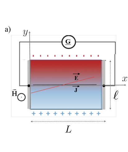
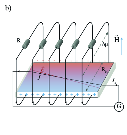
Figure 1: Schematic representation of a Hall-bar with the electrostatic charge accumulation $\pm\delta n$ at the edges, the electric field lines (red) and the current lines (black). The static magnetic field $H$ is applied along the $z$ direction. Note that the scales along $x$ and $y$ are not respected since we need $\ell\ll L$ in order to assume translational invariance along $x$. (a) planar Hall bar without dissipative leakage. (b) Same Hall bar including lateral circuit with transverse resistance $R_{H}$ and representation of the load resistance $R_{l}$ (preserving the translational invariance along $x$). The chemical potential difference $\Delta\mu$ is also represented.

II Joule dissipation

The system under interest is studied in the context of non-equilibrium thermodynamics Onsager ; Onsager_Diss ; Bruers ; MinDiss ; DeGroot ; Rubi . It is a thin homogeneous conducting layer of length $L$ and width $\ell$ contacted to an electric generator, and submitted to a constant magnetic field $\vec{H}$ oriented along the $z$ axis (see Fig.1). We assume that the conducting layer is planar, invariant by translation along the $x$ axis $\ell\ll L$ (this excludes the region in contact with the power generator), and the two lateral edges are symmetric.

Let us define the distribution of electric charge carriers by $n(y)=n_{0}+\delta n(y)$, where $\delta n(y)$ is the charge accumulation and $n_{0}$ the homogeneous density in the electrically neutral system (e.g. density of carriers without the magnetic field). The charge accumulation is governed by the Poisson’s equation $\nabla^{2}V=-\frac{q}{\varepsilon}\delta n$, where $V$ is the electrostatic potential, $q$ is the electric charge, and $\varepsilon$ is the electric permittivity. The local electrochemical potential $\mu(x,y)$ - that takes into account not only the electrostatic potential $V$ but also the energy (or the entropy) responsible for the diffusion - is given by the expression DeGroot ; Rubi (local equilibrium is assumed everywhere):

$$\mu=\frac{kT}{q}\ln\left(\frac{n}{n_{0}}\right)+V,$$ (1)

where $k$ is the Boltzmann constant and the temperature $T$ is the temperature of the heat bath in the case of a non-degenerate semiconductor, or the Fermi temperature $T_{F}$ in the case of a fully degenerate conductor Rque . Poisson’s equation now reads

$$\nabla^{2}\mu-\lambda_{D}^{2}\frac{q}{\varepsilon}n_{0}\nabla^{2}\ln\left(\frac{n}{n_{0}}\right)+\frac{q}{\varepsilon}\delta n=0,$$ (2)

where $\lambda_{D}=\sqrt{\frac{kT\varepsilon}{q^{2}n_{0}}}$ is the Debye-Fermi length. On the other hand, the transport equation under a magnetic field is given by the Ohm’s law:

$$\vec{J}=-\hat{\sigma}\vec{\nabla}\mu=-qn\hat{\eta}\vec{\nabla}\mu,$$ (3)

where the transport coefficients are the conductivity tensor $\hat{\sigma}$ or the mobility tensor $\hat{\eta}$. In two dimensions and for isotropic material, the mobility tensor is defined by Onsager relations Onsager :

$$\hat{\eta}=\begin{pmatrix}\eta&\eta_{H}\\ -\eta_{H}&\eta\end{pmatrix}=\eta\begin{pmatrix}1&\theta_{H}\\ -\theta_{H}&1\end{pmatrix}\quad\text{ with }\quad\theta_{H}=\frac{\eta_{H}}{\eta},$$

where $\eta$ is the ohmic mobility, $\eta_{H}$ the Hall mobility (usually proportional to the magnetic field $\vec{H}=H\vec{e}_{z}$) and $\theta_{H}$ the Hall angle. The electric current then reads:

$\vec{J}=-qn\eta\left(\vec{\nabla}\mu-\theta_{H}\,\vec{e_{z}}\times\vec{\nabla}\mu\right)$ (where $\times$ denotes the cross product), or:

$$-qn\eta(1+\theta_{H}^{2})\partial_{x}\mu =J_{x}-\theta_{H}J_{y}$$ (4)

$$-qn\eta(1+\theta_{H}^{2})\partial_{y}\mu =J_{y}+\theta_{H}J_{x}$$ (5)

$$\|\vec{J}\|^{2}\equiv J_{x}^{2}+J_{y}^{2} =(qn\eta)^{2}\,(1+\theta_{H}^{2})\,\|\vec{\nabla}\mu\|^{2}.$$ (6)

The expression of the Joule power dissipated by the system reads:

$$P_{J}=S_{\text{lat}}\int_{-\ell}^{\ell}qn\eta\|\vec{\nabla}\mu\|^{2}\differential{y}=\frac{L}{qn_{0}\eta(1+\theta_{H}^{2})}\int_{-\ell}^{\ell}\frac{n_{0}}{n}\|\vec{J}\|^{2}\differential{y}.$$

where $S_{\text{lat}}$ is the lateral surface of the Hall bar (product of the length $L$ by the thickness), and $2\ell$ is the width.

III The ideal Hall bar

The stationary state is defined by the least dissipation principle, that states that the current distributes itself so as to minimize Joule heating $P_{J}$ compatible with the constraints Onsager_Diss ; Bruers ; MinDiss .

Due to the symmetry of the device and the global charge conservation we have $\int_{-\ell}^{+\ell}\delta n\differential{y}=0$, and the total charge carrier density is constant $n_{\text{tot}}=\frac{1}{2\ell}\int n\differential{y}$. For the sake of simplicity, we assume a global charge neutrality so that $n_{\text{tot}}=n_{0}$. On the other hand, the global current flowing in the $x$ direction throughout the device is also constant along $x$ by definition of the galvanostatic condition. The two global constraints read:

$$\int_{-\ell}^{\ell}n(y)\differential{y}=2\ell n_{0}\quad\textrm{and}\quad\int_{-\ell}^{\ell}J_{x}(y)\differential{y}=2\ell J_{x}^{0}$$ (7)

We define for convenience the reduced power $\tilde{P_{J}}=\frac{q\eta(1+\theta_{H}^{2})}{S_{\text{lat}}}\,P_{J}=\int_{-\ell}^{\ell}\frac{J_{x}^{2}+J_{y}^{2}}{n}\differential{y}$. Let us introduce the two Lagrange multiplayers $\lambda_{J}$ and $\lambda_{n}$ corresponding to the two constraints Eqs(7). The functional to be minimized then reads:

$$\tilde{\mathcal{P}}_{J}[J_{x},J_{y},n]=\int_{-\ell}^{\ell}\left(\frac{J_{x}^{2}+J_{y}^{2}}{n}-\lambda_{J}\,J_{x}-\lambda_{n}\,n\right)\differential{y}$$ (8)

The minimum corresponds to:

$$\frac{\bm{\delta}\tilde{\mathcal{P}}_{J}}{\bm{\delta}J_{x}}=0\ \Longleftrightarrow\ 2J_{x}=n\lambda_{J},$$ (9)

$$\frac{\bm{\delta}\tilde{\mathcal{P}}_{J}}{\bm{\delta}J_{y}}=0\ \Longleftrightarrow\ J_{y}=0,$$ (10)

$$\frac{\bm{\delta}\tilde{\mathcal{P}}_{J}}{\bm{\delta}(n)}=0\ \Longleftrightarrow\ J_{x}^{2}+J_{y}^{2}=-\lambda_{n}n^{2},$$ (11)

Using Eqs.(7) and Eq.(9) leads to $\lambda_{J}=\frac{2J_{x}^{0}}{n_{0}}$ so that $J_{x}=\frac{n}{n_{0}}J_{x}^{0}$ (and from Eq.(11) we have furthermore : $\lambda_{n}=-(J_{x}^{0}/n_{0})^{2}$). Hence, the minimum is reached for

$$J_{x}(y)=J_{x}^{0}\frac{n(y)}{n_{0}}\quad\text{and}\quad J_{y}=0,$$ (12)

The usual stationarity condition $\vec{\nabla}\cdot\vec{J}=0$ is verified. Inserting the solution (12) into the transport equations (4,5), we deduce $\partial_{x}\mu=\frac{-J_{x}^{0}}{qn_{0}\eta(1+\theta_{H}^{2})}$ and $\partial_{y}\mu=\frac{\theta_{H}J_{x}^{0}}{qn_{0}\eta(1+\theta_{H}^{2})}$. These two terms are constant so that the electochemical potential of the stationary state is harmonic: $\nabla^{2}\mu=0$. Since the profile of the lateral current $J_{y}(y)$ is defined by the charge density $n(y)$, the Poisson’s equation Eq.(2) for $\nabla^{2}\mu=0$ gives the solution:

$$\lambda_{D}^{2}\partial_{y}^{2}\ln\left(1+\frac{\delta n}{n_{0}}\right)=\frac{\delta n}{n_{0}}.$$ (13)

Once again, the boundary conditions for the density $n$ are not defined locally but globally by Eq.(7), and by the integration of the Gauss’s law $\vec{\nabla}\cdot\vec{E}=\partial_{y}E_{y}=\frac{q}{\varepsilon}\delta n$, at a point $y_{0}$ (see Appendix C in reference JAP ):

$$E_{y}(y_{0})=-\partial_{y}V(y_{0})=-\frac{q}{2\varepsilon}\int_{-\ell}^{\ell}\delta n(y)\operatorname{sgn}(y-y_{0})\differential{y}+\Delta E^{\infty},$$ (14)

where the constant $\Delta E^{\infty}=E(+\infty)+E(-\infty)$ accounts for the electromagnetic environment of the Hall device ($\Delta E^{\infty}=0$ in vacuum) and the Sign function $\operatorname{sgn}(y-y_{0})\equiv(y-y_{0})/\absolutevalue{y-y_{0}}$ accounts for the opposite sign of the charge accumulation at both edges. Inserting the stationary solution (12) and the relation (5) for $\partial_{y}\mu$ gives the condition:

$$\frac{2\theta_{H}J_{x}^{0}C_{0}}{1+\theta_{H}^{2}}+2\lambda_{D}^{2}\partial_{y}\ln(\frac{n}{n_{0}})(y_{0})+2C_{E}+\int_{-\ell}^{\ell}\delta n(y)\operatorname{sgn}(y-y_{0})\differential{y}=0,$$ (15)

where $C_{0}=\frac{\varepsilon}{q^{2}n_{0}\eta}$ and $C_{E}=\frac{\varepsilon\Delta E^{\infty}}{qn_{0}}$. Using this condition and fixing $n_{0}$ gives a unique solution for $n(y)$, and the stationary current Eq.(12) is fully determined.

This derivation was the object of the report published in reference JAP , and the result was confirmed by an independent stochastic approachJAP2 . For small Debye length $\lambda_{D}/\ell\ll 1$, the charge accumulation $\pm\delta n$ at the edges give rise to the voltage $V_{H}^{0}=\frac{\theta_{H}2\ell J_{x}^{0}}{qn_{0}\eta}$. For low magnetic field $H$ we have $\theta_{H}\approx\eta H$ and the usual expression of the Hall voltage is recovered: $V_{H}^{0}=\frac{H2\ell J_{x}^{0}}{qn_{0}}$.

IV Effect of a lateral passive circuit

The solution found in the preceding section is valid as long as the dissipation due to charge leakage at the edges is negligible with respect to the dissipation inside the device. However, if it is no longer the case, the stationary regime should be reconsidered by introducing the dissipation due to the resistance of a lateral passive circuit that connects the edges of the Hall bar. In order to take into account this supplementary dissipation, we introduce the load conductivity $g$ ($\Omega^{-1}\cdot\mathrm{m}^{-2}$) of the lateral circuit (see Fig.1b). The power dissipated in the lateral circuit is, by definition of $g$:

$$P_{\text{lat}}\ =\ S_{\text{lat}}\,g\,\Delta\mu^{2}$$

where $\Delta\mu=\mu(+\ell)-\mu(-\ell)$ is the difference of the chemical potential between both edges (see Fig.1b). We assume that the load conductivity $g$ does not depend on the magnetic field. From a topological point of view, despite the presence of electric charge accumulation at the edges $\delta n\neq 0$, the fact that the system is doubly connected - instead of simply connected - suggests that the corresponding device is closer to a Corbino disk than a Hall bar Benda .
Note that due to our hypothesis of the invariance along $x$, we do not treat the case of a unique wire that joints the two edges of the Hall bar, that would form two “punctual” contacts on both edges (see Fig.1b). Indeed, such a contact would break the translation invariance symmetry along $x$, and would distort the current lines in a specific manner that depends on the details of the contact geometry and resistivity. Such a contact-specific effect is not related the generic problem studied here. Incidentally, it is well-known that the main advantage of the Corbino disk with respect to the Hall-bar device is precisely that it is much easier to design two quasi-perfect concentric equipotentials (circular symmetry) instead of two quasi-perfect longitudinal equipotentials (translational symmetry).

Using Eq.(5), the difference of chemical potential can be expressed as a function of the current:

$$\Delta\mu\ =\ \int_{-\ell}^{+\ell}\differential{y}\,\partial_{y}\mu\ =\ \int_{-\ell}^{+\ell}\differential{y}\,\frac{J_{y}+\theta_{H}J_{x}}{qn\eta(1+\theta_{H}^{2})}$$ (16)

so that

$$P_{\text{lat}}\ =\ \frac{S_{\text{lat}}\,g}{(q\eta)^{2}(1+\theta_{H}^{2})^{2}}\left(\int_{-\ell}^{+\ell}\differential y\frac{J_{y}+\theta_{H}J_{x}}{n}\right)^{2}$$ (17)

As in the preceding section, we define the reduced power $\tilde{P}=\frac{q\eta(1+\theta_{H}^{2})}{S_{\text{lat}}}P$. The total power dissipated is then:

$$\tilde{P}\ =\ \tilde{P}_{J}+\tilde{P}_{\text{lat}}\ =\ \int_{-\ell}^{+\ell}\differential y\frac{J_{x}^{2}+J_{y}^{2}}{n}\ +\ \alpha\left(\frac{n_{0}}{2\ell}\int_{-\ell}^{+\ell}\differential y\frac{J_{y}+\theta_{H}J_{x}}{n}\right)^{2}$$ (18)

where we have introduced the dimensionless control parameter $\alpha$:

$$\alpha=\frac{2\ell\,g}{q\eta n_{0}(1+\theta_{H}^{2})}$$ (19)

Note that the control parameter $\alpha$ is the ratio $\alpha=\frac{R_{H}}{R_{l}}$ of the “Hall resistance” per surface unit $R_{H}\equiv\frac{V_{H}}{J_{x}^{0}}=\frac{2\ell}{qn_{0}\eta(1+\theta_{H}^{2})}$ over the resistivity $R_{l}=\frac{1}{g}$ of the load.

Accordingly, the minimization of the corresponding functional $\tilde{\mathcal{P}}$ now reads:

$$\frac{\bm{\delta}\tilde{\mathcal{P}}}{\bm{\delta}J_{x}}=0\ \Longleftrightarrow\ 2\,\alpha\,A\,\theta_{H}+2J_{x}=n\lambda_{J},$$ (20)

where we have defined for convenience the constant $A\equiv\frac{n_{0}}{2\ell}\int_{-\ell}^{\ell}\frac{J_{y}+\theta_{H}J_{x}}{n}\differential{y}$. Furthermore:

$$\frac{\bm{\delta}\tilde{\mathcal{P}}}{\bm{\delta}J_{y}}=0\ \Longleftrightarrow\ \alpha\,A+J_{y}=0,$$ (21)

and

$$\frac{\bm{\delta}\tilde{\tilde{\mathcal{P}}}}{\bm{\delta}(n)}=0\ \Longleftrightarrow\ 2\alpha\,A+J_{x}^{2}+J_{y}^{2}=-\lambda_{n}\,n^{2},$$ (22)

Equations (20) and (22) define the Lagrange multipliers $\lambda_{J}$ and $\lambda_{n}$ and will not be used in the following. From Eq.(21) we can immediately deduce that :

• $J_{y}$ does not depend on $y$.

• In the absence of a magnetic field, $\theta_{H}=0$, and we have $\frac{n_{0}}{2\ell}\alpha\,J_{y}\int\tfrac{\differential y}{n}+J_{y}=0$, and $J_{y}=0$ is the unique solution (since $\alpha$ and $n$ are positive).

• If the load resistance goes to infinity $R_{l}\to\infty$ (or $g\to 0$), the power dissipated by the current leakage is negligible and we are back to the case discussed in the preceding section: the stationary state is defined by $J_{x}(y)=J_{x}^{0}\frac{n(y)}{n_{0}}$ and $J_{y}=0$.

• In the case of a short-circuit by the edges (i.e. the case of a Corbino disk), $R_{l}\to 0$ (or $g\to\infty$), we have $A\equiv\int\frac{J_{y}+\theta_{H}J_{x}}{n}\differential{y}\to 0$, which leads to the solution, at the limit: $J_{y}=-\theta_{H}J_{x}$. This is indeed the well-known stationary state for the Corbino disk, which corresponds to the maximum current $J_{y}$ Benda .

V Between Corbino disk and Hall bar

Introducing the constant current inside the integral of Eq.(21) with $J_{y}\equiv\int_{-\ell}^{+\ell}\frac{J_{y}\differential y}{2\ell}$, and dividing by $\frac{J_{y}}{2\ell}$ (for $J_{y}\neq 0$), we obtain

$$\int_{-\ell}^{+\ell}\differential y\left(1+\alpha\frac{n_{0}}{n}\left(1+\tfrac{\theta_{H}}{J_{y}}J_{x}\right)\right)\ =\ 0$$ (23)

As pointed-out above, the two limiting cases are solution of Eq.(23). At the limit of the perfect Hall bar (defined by an infinite load resistance and $\alpha=0$), a vanishing transverse current $J_{y}\rightarrow 0$ is recovered, while at the limit of the perfect Corbino disk (defined by $R_{l}=0$ or $\alpha=\infty$) the Corbino current $J_{y}=-\theta_{H}J_{x}$ is recovered. Without loss of generality, the solution $J_{y}(\alpha)$ can be expressed with introducing an arbitrary function $f(\alpha)$ such that $J_{y}=-f(\alpha)\,\theta_{H}J_{x}^{0}$. The function $f(\alpha)$ can be determined by using the sufficient condition

$$1+\alpha\frac{n_{0}}{n}\left(1+\theta_{H}\frac{J_{x}}{J_{y}}\right)=0.$$ (24)

We then obtain $J_{x}(y)=J_{x}^{0}\,f(\alpha)\left(1+\frac{1}{\alpha}\frac{n(y)}{n_{0}}\right)$. Applying the two global contraints Eqs.(7) leads to the expression $f(\alpha)=\frac{\alpha}{\alpha+1}\in\,[0,1]$, and thus to:

$$J_{y}=-\frac{\alpha}{\alpha+1}\theta_{H}J_{x}^{0}.$$ (25)

which interpolates the two limiting regimes for arbitrary ratio $\alpha=R_{H}/R_{\ell}$. From Eq.(24) we deduce:

$$J_{x}(y)=\frac{J_{x}^{0}}{\alpha+1}\left(\alpha+\frac{n(y)}{n_{0}}\right).$$ (26)

The lateral current $J_{y}$ is homogeneous (it does not depend on $y$), while the corresponding longitudinal current $J_{x}(y)$ is non-uniform and follows the profile of the charge accumulation $n(y)$. The relation $\vec{\nabla}\cdot\vec{J}=0$ is still verified, but the chemical potential is no longer harmonic. The derivative $\partial_{y}\mu=-\frac{J_{x}^{0}}{\alpha+1}\,\frac{\theta_{H}}{q\eta n_{0}(1+\theta_{H}^{2})}$ is still constant (decreased by a factor $1/(\alpha+1)$) while $\partial_{x}\mu(y)$ now depends on $y$. The typical profiles of the longitudinal and transverse currents Eq.(26) and Eq.(25) are plotted in Fig.2 in unit of the injected current $J_{x}^{0}$.

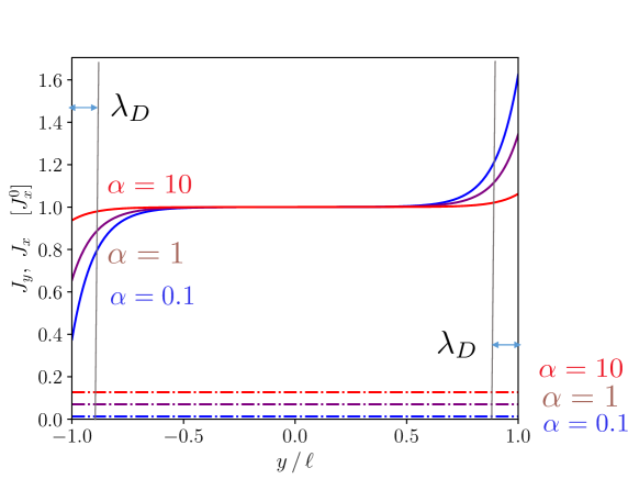
Figure 2: Typical profiles for the longitudinal current $J_{x}(y)$ (plain lines) and homogeneous transversal current $J_{y}$ (dotted horizontal lines) across the Hall-bar for various values of the parameter $\alpha=\{0.1,1,10\}$, and in units of the injected current $J_{x}^{0}$. The Debye length $\lambda_{D}$ is indicated by the vertical lines.

The Hall voltage with lateral load resistance can be derived easily. Inserting the solution Eqs.(25,26) instead of Eqs.(12) into Eq.(15), only the expression of the parameter $C_{0}$ is modified by the factor $1/(1+\alpha)$:

$$C_{0}(\alpha)=\frac{\epsilon}{q^{2}n_{0}\eta}\,\frac{1}{1+\alpha}$$ (27)

Assuming $C_{E}=0$, the charges accumulation $\delta n/n_{0}$ at the edges is reduced by the same factor:

$$\frac{\delta n(\alpha)}{n_{0}}=\,\frac{\mathcal{C}}{1+\alpha}$$ (28)

where $\mathcal{C}=\frac{\delta n}{n_{0}}(\alpha=0)$ is the charge accumulation without lateral circuit, as calculated in reference JAP :

$\mathcal{C}\equiv\frac{\theta_{H}J_{x}^{0}C_{0}}{n_{0}(1+\theta_{H}^{2})}\frac{1}{\lambda_{D}}\frac{\operatorname{sh}(y/\lambda_{D})}{\operatorname{ch}(y/(2\lambda_{D}))}$. For a vanishing screening length $\lambda_{D}\rightarrow 0$, the charge accumulation reduces to Dirac distributions at the edges of the Hall bar JAP :

$$q\,\delta n(y)=\sigma^{\mathsf{S}}\,\big{(}\delta\left(y-\ell\right)-\delta\left(y+\ell\right)\big{)}$$ (29)

where $\sigma^{\mathsf{S}}$ is the surface charge:

$$\sigma^{\mathsf{S}}(\alpha)=J_{x}^{0}\,\frac{\theta_{H}}{1+\theta_{H}^{2}}\frac{\varepsilon}{qn_{0}\eta}\frac{1}{1+\alpha},$$ (30)

that does not depend on $J_{y}$. Assuming the usual low magnetic field limit, we have $\theta_{H}\approx\eta H$ and the Hall voltage is deduced:

$$V_{H}(\alpha)=\frac{\sigma^{\mathsf{S}}L}{\varepsilon}=\frac{J_{x}^{0}HL}{qn_{0}}\frac{1}{1+\alpha}$$ (31)

The voltage Eq.(31) divided by Hall voltage $V_{H}^{0}$ of the ideal Hall bar is simply given by $\frac{V_{H}}{V_{H}^{0}}=\frac{1}{1+\frac{R_{H}}{R_{l}}}$, where we have replaced the parameter $\alpha$ by its value $\alpha=R_{H}/R_{l}$.

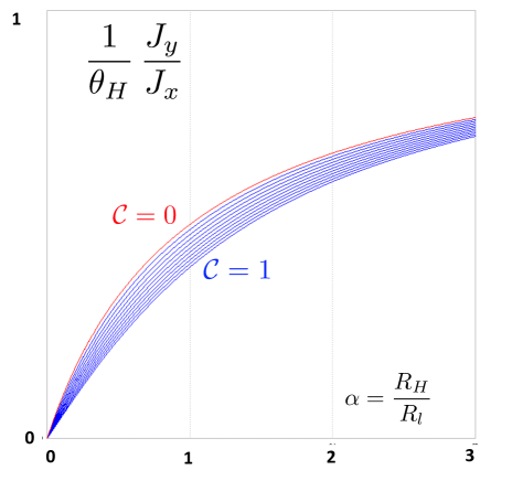
Figure 3: The ratio of the transverse current over longitudinal current divided by $\theta_{H}$: $J_{y}(\alpha)/\left(\theta_{H}\,J_{x}(\alpha)\right)$ at the edge ($y=\ell$) is plotted as a function of the parameter $\alpha=R_{H}/R_{l}$ for different values of the initial charge accumulation $\mathcal{C}=\delta n/n_{0}(\alpha=0)$ (varying from $0$ to $1$ with step $0.1$).

Note that the ratio if the transverse current over longitudinal current:

$$\frac{J_{y}}{J_{x}}(\alpha)=\frac{\theta_{H}\,\alpha}{\alpha+1+\frac{\mathcal{C}}{1+\alpha}}$$ (32)

is small for usual values of the angle $\theta_{H}$. This ratio divided by $\theta_{H}$ is plotted in Fig.3 at the edge $y=\ell$, as a function of $\alpha=R_{H}/R_{l}$. The quantitative study of the result Eq.(32) shows that the power injected into the lateral circuit is mainly carried by the longitudinal current $J_{x}(y)$ instead of the transverse current $J_{y}$. Indeed, as shown by Eq(29) and (30), the system can be interpreted as a capacitor which is recharged permanently by the longitudinal current $J_{x}$ only, in order to keep the charge accumulation $\delta n$ at stationary state. In other terms, the electric charges that are injected into the external circuit are mainly due to the discharge of the lateral edges, resupplied permanently by the longitudinal current $J_{x}$. This rather counter-intuitive picture invalidates that of a Hall current $J_{y}$ composed of carriers of charge carriers flowing transversally from one edge to the other through the Hall bar.

However, if the parameter $\alpha$ is large enough, the contribution of the transverse current $J_{y}$ to the total current becomes sizable for small values of the load resistance $R_{l}\ll R_{H}$ in nearly intrinsic semiconductors. Typically, the value of $\theta_{H}\approx 0.14$ is obtained in a field of $1\text{\,}\mathrm{T}$ in Silicon with impurity density of about $10^{15}$ $\mathrm{cm}^{-3}$. The transverse current $J_{y}$ injected into the lateral circuit can then reach the amplitude of the longitudinal current $J_{x}$ for a magnetic field of the order of $1\text{\,}\mathrm{T}$ if the coefficient $\alpha$ is of the order of $100$. The load circuit is then close to a short-circuit between the two edges of the Hall-bar, and the corresponding device is like a Corbino disk, i.e. a device in which the charge accumulation is not allowed.

VI Power injected

The total power $\tilde{P}=\tilde{P}_{J}+\tilde{P}_{\text{lat}}$ - given in Eq.(18) - is the sum of the Joule heating $\tilde{P}_{J}$ dissipated inside the Hall device, and the power $\tilde{P}_{\text{lat}}$ dissipated into the lateral passive circuit. Inserting the stationary state Eqs.(25,26) and using the first global condition in Eqs.(7), we obtain:

$$\tilde{P}(\alpha)=\frac{\left(J_{x}^{0}\right)^{2}}{(\alpha+1)^{2}}\left(\alpha^{2}(1+\theta_{H}^{2})\int_{-\ell}^{+\ell}\frac{\differential{y}}{n}+(2\alpha+1)\frac{2\ell}{n_{0}}+\frac{2\ell\alpha}{n_{0}}\theta_{H}^{2}\right)$$ (33)

Assuming that $\delta n\ll n_{0}$, we have $\int_{-\ell}^{+\ell}\frac{\differential{y}}{n(y)}\simeq 2\ell/n_{0}$ and the total dissipated power reads:

$$P_{\text{tot}}(\alpha)\,\simeq\,\frac{2\ell\left(J_{x}^{0}\right)^{2}}{q\eta n_{0}}\,\frac{\alpha^{2}(1+\theta_{H}^{2})+\alpha(2+\theta_{H}^{2})+1}{(\alpha+1)^{2}}\,=\,P(0)\,\left(1+\theta_{H}^{2}\frac{\alpha}{\alpha+1}\right)$$ (34)

where $P(0)$ is the power dissipated by the ideal Hall-bar without lateral contact.

On the other hand, the power injected into the lateral circuit is

$$P_{\text{lat}}(\alpha)=P(0)\,\left(\theta_{H}^{2}\frac{\alpha}{(\alpha+1)^{2}}\right)$$ (35)

The total power dissipated in the lateral circuit Eq.(34) normalized by $P(0)$ is plotted in Fig.4(a) and the power injected into the lateral circuit Eq.(35) normalized by $P(0)$ is plotted in Fig.4(b), as a function of $\alpha=R_{H}/R_{l}$. The different profiles corresponds to different values of $\theta_{H}$ from $0$ to $0.1$. Due to the small values of the Hall angle $\theta_{H}$, the power injected into the lateral circuit is a small fraction of the total power dissipated by the device. The ratio $P_{\text{lat}}/P_{\text{tot}}$ - i.e. the efficiency of the injection - is indeed proportional to $\theta_{H}^{2}$.

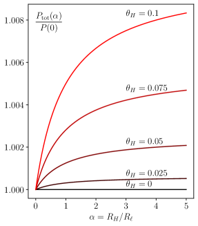
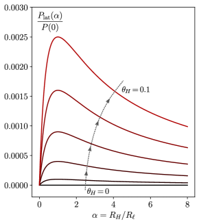
(a)                 (b)

Figure 4: Amplification of the power as a function of $\alpha=R_{H}/R_{l}$ for different values of the Hall angle $\theta_{H}$ (i.e. of the static magnetic field $H$) from $0$ to $0.1$. (a) Total power $P_{\text{tot}}$ dissipated in the device normalized by the power without lateral circuit $P(0)$. (b) Power $P_{\text{lat}}$ injected in the lateral circuit normalized by the power without lateral circuit $P(0)$. The maximum coincides with the resistance matching $R_{\ell}=R_{H}$.

Note that in Fig.4(b) the power injected into the lateral circuit reaches a maximum at $\alpha=1$, i.e. for $R_{\ell}=R_{H}$, independently of the magnetic field. Indeed, the situation is analogous to a voltage source with internal resistance $R_{H}$, loaded with $R_{\ell}$. The expression $P_{\text{lat}}(R_{\ell})$ is then an illustration of the so called maximum power transfer theorem, where the maximal injected power is achieved at the impedance matching condition $R_{\ell}=R_{H}$. This observation gives an intuitive meaning of the Hall resistance $R_{H}$ as the internal resistance of a voltage source, when the Hall bar is used as the power supply for a lateral circuit.

VII CONCLUSION

We have performed a quantitative analysis of the stationary state of a Hall-bar connected to a load circuit at the lateral edges. This configuration corresponds to the so-called current mode of Hall devices. This analysis is based on a variational approach developed in previous works. The model assumes a planar device, a perfect symmetry of the two lateral edges, and a translational invariance along the longitudinal direction $x$ (the deformation of the current lines due to the contacts is not taken into account). The expression of the non-uniform longitudinal current $J_{x}(y)$ is calculated. This current allows the charge accumulation to be maintained at stationary state. When a lateral circuit is connected to the lateral edges of the Hall-bar, it is shown that the current $J_{x}(y)$ is amplified and a Hall current is generated: $J_{y}\neq 0$. The power injected from the Hall bar to the lateral circuit can be controlled by the magnetic field and by the load resistance $R_{\ell}$. It is shown that the physical significance of the Hall resistance $R_{H}$ is that of the usual internal resistance of a voltage source, when the Hall bar is used as the power supply for the lateral circuit.

Beyond, the surprising result of this study is that, for usual values of the Hall angle, the main contribution of the power injected into the lateral circuit is due to the longitudinal current $J_{x}$ instead of the transverse current $J_{y}$. This means that the device can be interpreted as a capacitor which is recharged permanently by the longitudinal current $J_{x}$ only, in order to keep the charge accumulation $\delta n$ at stationary state. In other terms, the electric charges that are injected into the external circuit are mainly due to the discharge of the lateral edges, resupplied permanently by the longitudinal current $J_{x}$. This rather counter-intuitive picture invalidates that of a Hall current $J_{y}$ composed of charge carriers flowing transversally from one edge to the other through the Hall bar. However, this more intuitive Hall-current regime with sizable $J_{y}$ is able to take place for nearly intrinsic semiconductors (for which $\theta_{H}\approx 0.15$ or above), for small enough load resistance $R_{ell}<(R_{H}/100)$: the device is then close to a Corbino disk. The two different regimes are then able to take place in the same device, depending on the values of the load resistance $R_{\ell}$.

References

- (1) E. H. Hall On a new action of the magnet on electric currents, Am. J. Math. 2, 287 (1879).
- (2) O. Corbino, Elektromagnetische effekte, die von der verzerrung herrühren, welche ein feld and der bahn der ionen in metallen hervorbringt, Phyz. Z 12, 561 (1911).
- (3) N. W. Ashcroft and N. D. Mermin, Solid State Physics, Holt-Saunders, Philadelphia, 1976: page 12.
- (4) Ch. Kittel, Introduction to solid state physics, Ed. Wiley, Eighth Edition (2008), Chapter 6 p153 and explicitly page 499.
- (5) R. Benda, E. Olive, M. J. Rubì and J.-E. Wegrowe Towards Joule heating optimization in Hall devices, Phys. Rev. B 98, 085417 (2018).
- (6) M. Creff, F. Faisant, M. Rubì, J.-E. Wegrowe surface current in Hall devices, J. Appl. Phys. 128, 054501 (2020). https://doi.org/10.1063/5.0013182.
- (7) P.-M. Déjardin and J-E. Wegrowe Stochastic description of the stationary Hall effect, J. Appl. Phys. 128, 184504 (2020)
- (8) B. Madon, M. Hehn, F. Montaigne, D. Lacour, and J.-E. Wegrowe. Corbino magnetoresistance in ferromagnetic layers : Two representative examples and Phys. Rev B (R) 98 220405(R) (2018).
- (9) J.-E. Wegrowe, R. V. Benda, and J. M. Rubì., Conditions for the generation of spin current in spin-Hall devices, Europhys. Lett 18 67005 (2017).
- (10) J.-E. Wegrowe, P.-M. Dejardin, Variational approach to the stationary spin-Hall effect, Europhys. Lett 124, 17003 (2018).
- (11) R.S. Popovic, Hall Effect Devices, IoP Publishing, Bristol and Philadelphia 2004 (Second Edition): Chapter 4, Paragraph 4.4: The Hall current mode of operation .
- (12) H. Heidari, E. Bonizzoni, F. Maloberti, A CMOS Current-Mode Magnetic Hall Sensor With Integrated Front-End, IEEE Trans. Circuits Syst. 62, 2015.
- (13) Yue Xu, Xingxing Hu and Lei Jiang An Analytical Geometry Optimization Model foe Current-Mode Cross-Like Hall Plates, Sensors 19, 2490 (2019) .
- (14) L. Onsager Reciprocal relations in irreversible processes II, Phys. Rev. 38, 2265 (1931)
- (15) L. Onsager and S. Machlup, Fluctuations and irreversible processes, Phy. Rev. 91 1505 (1953).
- (16) S. Bruers, Ch. Maes, K. Netocný, On the validity of entropy production principles for linear electrical circuits, J. Stat. Phys. 129, 725 (2007).
- (17) L. Bertini, A. De Sole, D. Gabrielli, G. Jona-Lasinio, and C. Landim Minimum Dissipation Principle in Stationary Non-Equilibrium Sates, J. Stat. Phys. 116, 831 (2004).
- (18) See the sections relaxation phenomena and internal degrees of freedom in Chapter 10 of De Groot, S.R.; Mazur, P. Non-equilibrium Thermodynamics; North-Holland: Amsterdam, The Netherlands, 1962.
- (19) D. Reguera, J. M. G. Vilar, and J. M. Rubì, The mesoscopic Dynamics of Thermodynamic Systems, J. Phys. Chem. B 109 (2005).
- (20) The expression is valid for non-degenerate semiconductor (Maxwellian distribution). However, in the case of degenerate metal, the expression is an approximation for .