Deterministic and Probabilistic Error Bounds for Floating Point Summation Algorithms

Abstract

We analyse the forward error in the floating point summation of real numbers, from algorithms that do not require recourse to higher precision or better hardware. We derive informative explicit expressions, and new deterministic and probabilistic bounds for errors in three classes of algorithms: general summation, shifted general summation, and compensated (sequential) summation. Our probabilistic bounds for general and shifted general summation hold to all orders. For compensated summation, we also present deterministic and probabilistic first and second order bounds, with a first order bound that differs from existing ones. Numerical experiments illustrate that the bounds are informative and that among the three algorithm classes, compensated summation is generally the most accurate method.

65G99, 60G42, 60G50

1 Introduction

Given $n$ real numbers $x_{1},\ldots,x_{n}$, we consider algorithms for summation $s_{n}=x_{1}+\cdots+x_{n}$ in floating point arithmetic. The algorithms operate in one and only one precision, without any recourse to higher precision as in [1], or wider accumulators as in [6].

We analyze the forward error $e_{n}=\hat{s}_{n}-s_{n}$ in the computed sum $\hat{s}_{n}$ in terms of the unit roundoff $u$, for three classes of algorithms: general summation (Section 2), shifted general summation (Section 3), and compensated summation (Section 4). Numerical experiments (Section 5) illustrate that the bounds are informative, and that, among the three classes of algorithms, compensated summation is the most accurate method. Hybrid algorithms as in [1] will be analyzed in future work.

1.1 Contributions

We present informative bounds, based on clear and structured derivations, for three classes of summation algorithms.

General summation

We derive explicit expressions for the error (Lemmas 2.2 and 2.3); as well as deterministic bounds that hold to all orders (Theorem 2.4) and depends on the height $h$ of the computational tree associated with the particular summation order. We present two probabilistic bounds that treat the roundoffs as random variables, one for independent roundoffs (Theorem 2.8) and one for mean-independent roundoffs (Theorem 2.12). Both bounds hold to all orders, depend only on $\sqrt{h}$, and suggest that reducing the tree height $h$ increases the accuracy.

Shifted general summation

We present the extension of shifted sequential summation to shifted general summation (Algorithm 2). For the special case of shifted sequential summation we present an explicit expression for the error, and a simple probabilistic bound for independent roundoffs (Theorem 3.2). For shifted general summation, we deduce probabilistic bounds for mean-independent roundoffs (Theorem 3.4) and independent roundoffs (Theorem 3.6) as respective special cases of Theorems 2.12 and 2.8.

Compensated summation

We derive three different explicit expressions for the error (Theorems 4.3 and 4.5), and bounds that are valid to first and second order, both deterministic (Corollary 4.6, Theorem 4.9) and probabilistic (Theorem 4.11, Corollary 4.13). In particular (Remark 4.8) we note the discrepancy by a factor $u$ of existing bounds with ours in Corollary 4.6,

$$|\hat{s}_{n}-s_{n}|\leq 3u\,\sum_{k=1}^{n}{|x_{k}|}+\mathcal{O}(u^{2}).$$

1.2 Models for roundoff error

Our analyses assume that the inputs $x_{k}$ are floating point numbers, i.e. can be stored exactly without error, and that the summation produces no overflow or underflow.

Let $u$ denote the unit roundoff.

Standard model [9]

This holds for IEEE floating-point arithmetic and implies that in the absence of underflow or overflow, the operations $\text{op}\in\{+,-,\times,/,\sqrt{}\}$ when applied to floating point inputs $x$ and $y$ produce

(1) $$\operatorname*{fl}(x\text{ op }y)=(x\text{ op }y)(1+\delta_{xy}),\qquad|\delta_{xy}|\leq u.$$

In order to derive probabilistic bounds, we treat the roundoffs as zero-mean random variables, according to two models that differ in the assumption of independence.

Model 1.1.

In the computation of interest, the quantities $\delta_{xy}$ in the model (1) associated with every pair of operands are independent random variables of mean zero.

Model 1.2.

Let the computation of interest generate rounding errors $\delta_{1},\delta_{2},\ldots$ in that order. The $\delta_{k}$ are random variables of mean zero such that

$$\mathbb{E}(\delta_{k}|\delta_{1},\ldots,\delta_{k-1})=\mathbb{E}(\delta_{k})=0.$$

Higham and Mary [11] note that the mean independence assumption of Model 1.2 is weaker than the independence assumption of Model 1.1, but stronger than the assumption that the errors are uncorrelated. Connolly, et al. [3] observe that at least one mode of stochastic rounding produces errors satisfying Model 1.2, but with the weaker bound $|\delta_{xy}|\leq 2u$ in place of (1).

1.3 Probability theory

For the derivation of the probabilistic bounds, we need a martingale, and a concentration inequality.

Definition 1.1 (Martingale [18]).

A sequence of random variables $Z_{1},\ldots,Z_{n}$ is a martingale with respect to the sequence $X_{1},\ldots,X_{n}$ if, for all $k\geq 1$,

• $Z_{k}$ is a function of $X_{1},\ldots,X_{k}$,

• $\mathbb{E}[|Z_{k}|]<\infty$, and

• $\mathbb{E}(Z_{k+1}|X_{1},\ldots,X_{k})=Z_{k}$.

Lemma 1.2 (Azuma-Hoeffding inequality [20]).

Let $Z_{1},\ldots,Z_{n}$ be a martingale with respect to a sequence $X_{1},\ldots,X_{n}$, and let $c_{k}$ be constants with

$$|Z_{k}-Z_{k-1}|\leq c_{k},\qquad 2\leq k\leq n.$$

Then for any $\delta\in(0,1)$, with probability at least $1-\delta$,

(2) $$|Z_{n}-Z_{1}|\leq\left(\sum_{k=2}^{n}c_{k}^{2}\right)^{1/2}\sqrt{2\ln(2/\delta)}.$$

If the bounds on the differences $|Z_{k}-Z_{k-1}|$ are permitted to fail with a small probability, then a similar but weaker concentration inequality holds [2]. Specifically, if $|Z_{k}-Z_{k-1}|\leq c_{k}$ simultaneously for all $2\leq k\leq n$ with exceptional probability at most $\eta$, then (2) still holds with probability at least $1-(\delta+\eta)$.

2 General summation

We analyse the error for general summation, presented in Algorithm 1. After representing the summation algorithm as a computational tree, we present error expressions and a deterministic error bound (Section 2.1), deterministic and probabilistic bounds valid to first order (Section 2.2), followed by two probabilistic bounds, one for Model 1.1 (Section 2.3) and one for Model 1.2 (Section 2.4).

Algorithm 1 General Summation [9, Algorithm 4.1]

0:  A set of floating point numbers $\mathcal{S}=\{x_{1},\ldots,x_{n}\}$

0:  $s_{n}=\sum_{k=1}^{n}{x_{k}}$

1:  for $k=2:n$ do

2:     Remove two elements $x$ and $y$ from $\mathcal{S}$

3:     $s_{k}=x+y$

4:     Add $s_{k}$ to $\mathcal{S}$

5:  end for

Denote by $s_{k}$ the exact partial sum, by $\hat{s}_{k}$ the computed sum, and by $e_{k}=\hat{s}_{k}-s_{k}$ the forward error, $2\leq k\leq n$.

Computational tree for Algorithm 1

We represent the specific ordering of summations in Algorithm 1 by a binary tree with $2n-1$ vertices and the following properties:

• Each vertex represents a partial sum $s_{k}$ or an input $x_{k}$.

• Each operation $s_{k}=x+y$ gives rise to two edges $(x,s_{k})$ and $(y,s_{k})$.

• The root is the output $s_{n}$, and the leaves are the inputs $x_{1},\ldots,x_{n}$.

Figure 1 shows two examples, one for sequential (recursive) summation and one for pairwise summation.

Figure 1: Computational trees for two different summation orderings in Algorithm 1 when $n=4$. Left: sequential (recursive) summation. Right: pairwise summation.

Definition 2.1.

Consider the computational tree associated for Algorithm 1 applied to $n$ inputs.

• The tree defines a partial ordering. If $s_{j}$ is a descendant of $s_{k}$, we say $j\prec k$ and $j\preceq k$ if $s_{j}=s_{k}$ is possible.

• The height of a node is the length of the longest downward path from that node to a leaf. Leaves have a height of zero.

• The height of the tree is the height of its root. Sequential (recursive) summation yields a tree of height $n-1$, while pairwise summation yields a tree of height $\lceil\ln_{2}n\rceil$, see Figure 1.

2.1 Explicit expressions and deterministic bounds for the error

We present two expressions for the error in Algorithm 1 (Lemmas 2.2 and 2.3) each geared towards a different model for the subsequent probabilistic bounds; and two deterministic bounds (Theorem 2.4).

If the computed children are $\hat{x}=x+e_{x}$ and $\hat{y}=y+e_{y}$, then the computed parent sum, in line 3 of Algorithm 1, is

$$\hat{s}_{k}=(\hat{x}+\hat{y})(1+\delta_{k}),\qquad 2\leq k\leq n.$$

Highlight the error in the children,

$$s_{k}+e_{k}=\hat{s}_{k}=((x+e_{x})+(y+e_{y}))(1+\delta_{k})=(s_{k}+e_{x}+e_{y})(1+\delta_{k})$$

to obtain the error in the parent

(3) $$e_{k}=(s_{k}+e_{x}+e_{y})(1+\delta_{k})-s_{k}=(e_{x}+e_{y})(1+\delta_{k})+s_{k}\delta_{k},\qquad 2\leq k\leq n.$$

This means the error at node $s_{k}$ equals the sum of the children errors, perturbed slightly, plus a local error that is proportional to the exact partial sum $s_{k}$.

The unravelled recursions in Lemma 2.2 generalize the explicit expressions for sequential (recursive) summation in [8, Lemma 3.1],

(4) $$e_{n}=\hat{s}_{n}-s_{n}=\sum_{k=2}^{n}{s_{k}\delta_{k}\prod_{\ell=k+1}^{n}{(1+\delta_{\ell})}}$$

to general summation algorithms.

We present two expressions that differ in their usefulness under particular probabilistic models. The expression in Lemma 2.2 works well with Model 1.1 because the sum is a martingale if summed in reverse order, see Section 2.3. Unfortunately, this approach does not work under the weaker Model 1.2. This is the reason for Lemma 2.3 where the sum is a martingale under the original ordering, see Section 2.4.

Lemma 2.2 (First explicit expression).

The error in Algorithm 1 equals

(5) $$e_{n}=\hat{s}_{n}-s_{n}=\sum_{k=2}^{n}s_{k}\delta_{k}\prod_{k\prec j\preceq n}(1+\delta_{j}).$$

This means the forward error is the sum of the local errors at each node, each perturbed by subsequent rounding errors. A similar expression is derived in [9, (4.2)]

(6) $$e_{n}=\sum_{k=2}^{n}\hat{s}_{k}\tilde{\delta}_{k},$$

but in terms of the computed partial sums $\hat{s}_{k}$. By contrast, our (5) depends only on the exact partial $s_{k}$, which make it more amenable to a probabilistic analysis.

Write (3) in terms of the sum $f_{k}$ of the children errors at node $s_{k}$,

$$e_{k}=f_{k}+(s_{k}+f_{k})\delta_{k},\qquad f_{k}\equiv e_{x}+e_{y},\qquad 2\leq k\leq n.$$

Unraveling the recurrence gives the second explicit expression for the errors.

Lemma 2.3 (Second explicit expression).

The errors in Algorithm 1 equal

(7) $$e_{k}=\hat{s}_{k}-s_{k}=\sum_{j\preceq k}(s_{j}+f_{j})\delta_{j},\qquad 2\leq k\leq n,$$

and similarly

(8) $$f_{k}=\sum_{j\prec k}(s_{j}+f_{j})\delta_{j},\qquad 2\leq k\leq n.$$

Theorem 2.4.

If $h$ is the height of the computational tree for Algorithm 1, the error is bounded by

$$|e_{n}| \leq\sum_{k=2}^{n}|s_{k}||\delta_{k}|\left|\prod_{k\prec j\preceq n}(1+\delta_{j})\right|\leq u(1+u)^{h}\sum_{k=2}^{n}|s_{k}|$$

$$\leq\frac{h^{2}u^{2}}{1-hu}\,\sum_{k=1}^{n}{|x_{k}|},\qquad\mathrm{provided}~{}hu<1.$$

Proof 2.5.

The first bound is a direct consequence of Lemma 2.2. The second one follows from $\sum_{k=2}^{n}|s_{k}|\leq h\sum_{k=1}^{n}|x_{k}|$, and $(1+u)^{h}\leq hu/(1-hu)$ [9, Lemma 3.1].

A similar bound is derived from (6) in [9, (4.3)],

$$|e_{n}|\leq u\sum_{k=2}^{n}|\hat{s}_{k}|,$$

is accompanied by the following observation:

In designing or choosing a summation method to achieve high accuracy, the aim should be to minimize the absolute values of the intermediate sums $s_{k}$.

Our probabilistic bounds in Sections 2.3 and 2.4 corroborate this observation, the main difference being a dependence on $\left(\sum_{k}s_{k}^{2}\right)^{1/2}$ rather than $\sum_{k}|s_{k}|$.

2.2 Deterministic and probabilistic error bounds valid to first order

We present a deterministic bound (9), and a probabilistic bound (Theorem 2.6) under Model 1.2, both valid to first order.

Truncating in Theorem 2.4 yields the first order bound

(9) $$e_{n}=\sum_{k=2}^{n}s_{k}\delta_{k}+\mathcal{O}(h^{2}u^{2}),$$

which is also derived in [11, Lemma 2.1] for the special case sequential (recursive) summation.

Theorem 2.6.

Let $\delta_{2},\ldots,\delta_{n}$ be mean-indepen-dent, zero mean random variables. Then for any $\delta\in(0,1)$, with probability at least $1-\delta$, the error in Algorithm 1 is bounded by

$$|e_{n}|\leq u\left(\sum_{k=2}^{n}s_{k}^{2}\right)^{1/2}\sqrt{2\ln(2/\delta)}+\mathcal{O}(u^{2}).$$

Proof 2.7.

With $\delta_{1}=0$, the sequence $Z_{1}=0$, $Z_{i}=\sum_{k=2}^{i}s_{k}\delta_{k}$, $2\leq i\leq n$, is a martingale with respect to $\delta_{1},\ldots,\delta_{n}$, satisfying

$$|Z_{i}-Z_{i-1}|\leq u|s_{k}|,\qquad 2\leq i\leq n.$$

Now apply Lemma 1.2.

A closely related bound for sequential (recursive) summation is derived in [11, Theorem 2.8] under a model where the inputs $x_{k}$ are themselves random variables. Under this assumption, the probabilistic error bounds become significantly tighter if $\mathbb{E}[x_{k}]=0$, leading to the conclusion that centering the data prior to summation can reduce the error, see Section 3.

A disadvantage of Theorem 2.6 is its uncertainty about the point where the second-order term $\mathcal{O}(u^{2})$ starts to become relevant. For input dimensions $n>u^{-1}$ or $h>u^{-1}$ in particular, it is desirable to derive bounds that hold to all orders.

2.3 General probabilistic bound under Model 1.1

We derive a bound under the assumption of independent roundoffs $\delta_{2},\ldots,\delta_{n}$.

Theorem 2.8.

Let $\delta_{2},\ldots,\delta_{n}$ be independent zero-mean random variables, $h$ the height of the computational tree for Algorithm 1, and $\lambda\equiv\sqrt{2\ln(2n/\eta)}$. Then for any $\delta\in(0,1)$ and $\eta\in(0,1)$, with probability at least $1-(\delta+\eta)$, the error in Algorithm 1 is bounded by

$$|\hat{s}_{n}-s_{n}|\leq u\exp(\lambda\sqrt{h}u)\left(\sum_{k=2}^{n}{s_{k}^{2}}\right)^{1/2}\sqrt{2\ln(2/\delta)}.$$

Proof 2.9.

We start by bounding the products in the error expression (5). Since

$$\prod_{k\prec j\preceq n}(1+\delta_{j})\leq\exp\left(\sum_{k\prec j\preceq n}\delta_{j}\right),\qquad 2\leq k\leq n-1,$$

we can apply Lemma 1.2 to the sum on the right to conclude that for each $k$, $\eta\in(0,1)$, and $\lambda=\sqrt{2\ln(2/\eta)}$ with failure probability at most $\eta$, the bound

$$\prod_{k\prec j\preceq n}(1+\delta_{j})\leq\exp(\lambda\sqrt{h}u)$$

holds. Since the product is nonnegative, we can replace the expression on the left with its absolute value and the statement still holds. A union bound over at most $n$ such inequalities shows that with failure probability at most $n\cdot\eta$ the bound

$$\max_{2\leq k\leq n}\left|\prod_{k\prec j\preceq n}(1+\delta_{j})\right|\leq\exp(\lambda\sqrt{h}u)$$

holds. Then substitute $\eta\mapsto\eta/n$ and $\lambda=\sqrt{2\ln(2n/\eta)}$.

Next, with $\delta_{1}=0$, the sequence

$$Z_{1}=0,\qquad Z_{i}=\sum_{k=n-i+2}^{n}s_{k}\delta_{k}\prod_{k\prec j\preceq n}(1+\delta_{j}),\qquad 2\leq i\leq n$$

is a martingale with respect to $\delta_{n},\delta_{n-1},\ldots,\delta_{2}$, that satisfies

$$|Z_{i}-Z_{i-1}|\leq u\exp(\lambda\sqrt{h}u)|s_{n-i+2}|,\qquad 2\leq i\leq n$$

with failure probability at most $\eta$. At last apply Lemma 1.2 with additional failure probability $\delta$.

The bound $\left(\sum_{k=2}^{n}s_{k}^{2}\right)^{1/2}\leq\sqrt{h}\sum_{i=1}^{n}|x_{i}|$ illustrates that, with high probability, the error in Theorem 2.8 is bounded by a quantity proportional to the square root of the height of the computational tree in Algorithm 1. This suggests that minimizing the height of the computational tree should reduce the error.

As long as $\lambda\sqrt{h}u\ll 1$, the probability $\eta$ can be made small, without much effect on the overall bound in Theorem 2.8.

2.4 General probabilistic bound under Model 1.2

We derive a bound under the assumption of mean-independent roundoffs $\delta_{2},\ldots,\delta_{n}$. To this end we rely on the recurrence in (8) and induction.

Lemma 2.10.

Let $\delta_{2},\ldots,\delta_{n}$ be mean-independent mean-zero random variables, $h$ the height of the computational tree for Algorithm 1, and $\lambda\equiv\sqrt{2\ln(2n/\eta)}$. For any $\eta>0$ with $\lambda\sqrt{h}u<1$, the bounds

(10) $$|f_{k}|\leq\frac{\lambda u}{1-\lambda\sqrt{h}u}\left(\sum_{j\prec k}s_{j}^{2}\right)^{1/2},\qquad 2\leq k\leq n$$

all hold simultaneously with probability at least $1-\eta$.

Proof 2.11.

The proof is by induction, and in terms of the failure probability $\eta$.

Induction basis $k=2$

The children of $s_{2}$ are both leaves and floating point numbers, hence $f_{2}=0$ and (10) holds deterministically.

Induction hypothesis

Assume that (10) holds simultaneously for all $2\leq j\leq k-1$ with failure probability at most $(k-1)\eta/n$.

Induction step

Write (8) as

$$f_{k}=\sum_{j=2}^{k-1}(s_{j}+f_{j})\delta_{j}\mathds{1}_{j\prec k}.$$

With $\delta_{1}=0$, the sequence $Z_{1}=0$, $Z_{i}=\sum_{j=2}^{i}(s_{j}+f_{j})\delta_{j}\mathds{1}_{j\prec k}$ is a martingale with respect to $\delta_{1},\ldots,\delta_{k-1}$, and by the induction hypothesis satisfies

$$|Z_{i}-Z_{i-1}|\leq\begin{cases}us_{i}+\frac{\lambda u^{2}}{1-\lambda\sqrt{h}u}\left(\sum_{j\prec i}s_{j}^{2}\right)^{1/2}&i\prec k,\\ 0&i\nprec k,\end{cases},\qquad 2\leq i\leq k-1,$$

with failure probability at most $(k-1)\eta/n$. Lemma 1.2 then implies that with additional failure probability $\eta/n$,

$$|f_{k}| \leq\lambda u\left(\sum_{j\prec k}\left(s_{j}+\frac{\lambda u}{1-\lambda\sqrt{h}u}\Big{(}\sum_{\ell\prec j}s_{\ell}^{2}\Big{)}^{1/2}\right)^{2}\right)^{1/2}$$

$$\leq\lambda u\left(\sum_{j\prec k}s_{j}^{2}\right)^{1/2}+\lambda u\left(\sum_{j\prec k}\left(\frac{\lambda u}{1-\lambda\sqrt{h}u}\Big{(}\sum_{\ell\prec j}s_{\ell}^{2}\Big{)}^{1/2}\right)^{2}\right)^{1/2}$$

where the second inequality follows from the two-norm triangle inequality. Exploit the fact that $s_{j}$ can appear at most $h$ times, once for itself and once for each of its ancestors, to bound the second summand by

$$\lambda u\left(\sum_{j\prec k}\left(\frac{\lambda u}{1-\lambda\sqrt{h}u}\Big{(}\sum_{\ell\prec j}s_{\ell}^{2}\Big{)}^{1/2}\right)^{2}\right)^{1/2} =\frac{\lambda^{2}u^{2}}{1-\lambda\sqrt{h}u}\left(\sum_{j\prec k}\sum_{\ell\prec j}s_{\ell}^{2}\right)^{1/2}$$

$$\leq\frac{\lambda^{2}u^{2}}{1-\lambda\sqrt{h}u}\left(h\sum_{j\prec k}s_{j}^{2}\right)^{1/2}.$$

Combine everything

$$|f_{k}| \leq\lambda u\left(\sum_{j\prec k}s_{j}^{2}\right)^{1/2}+\frac{\lambda^{2}u^{2}}{1-\lambda\sqrt{h}u}\left(h\sum_{j\prec k}s_{j}^{2}\right)^{1/2}$$

$$=\lambda u\left(1+\frac{\lambda\sqrt{h}u}{1-\lambda\sqrt{h}u}\right)\left(\sum_{j\prec k}s_{j}^{2}\right)^{1/2}=\frac{\lambda u}{1-\lambda\sqrt{h}u}\left(\sum_{j\prec k}s_{j}^{2}\right)^{1/2}.$$

Thus (10) holds simultaneously for all $2\leq j\leq k$ with failure probability at most $k\eta/n$. By induction (10) holds for all $2\leq k\leq n$ with failure probability at most $\eta$.

Below is the final probabilistic bound under Model 1.2.

Theorem 2.12.

Let $\delta_{2},\ldots,\delta_{n}$ be mean-independent mean-zero random variables, $h$ the height of the computational tree for Algorithm 1, and $\lambda\equiv\sqrt{2\ln(2n/\eta)}$. For any $\eta>0$ with $\lambda\sqrt{h}u<1$ and $\delta\in(0,1)$, with probability at least $1-(\delta+\eta)$, the error in Algorithm 1 is bounded by

(11) $$|\hat{s}_{n}-s_{n}|\leq\frac{u}{1-\lambda\sqrt{h}u}\left(\sum_{k=2}^{n}s_{k}^{2}\right)^{1/2}\sqrt{2\ln(2/\delta)}.$$

Proof 2.13.

Apply Lemma 1.2 to (7) with failure probability $\delta$, and bound $|f_{k}|$ with Lemma 2.10.

The bound in Theorem 2.12 is nearly identical to the one in Theorem 2.8, the difference becoming significant only when $\lambda\sqrt{h}u$ is close to 1.

3 Shifted General Summation

After discussing the motivation for shifted summation, we present Algorithm 2 for shifted general summation; and derive error expressions, deterministic and probabilistic bounds for shifted sequential (recursive) summation (Section 3.1) and shifted general summation (Section 3.2).

Shifted summation is motivated by work in computer architecture [5, 4] and formal methods for program verification [17] where not only the roundoffs but also the inputs are interpreted as random variables sampled from some distribution. Then one can compute statistics for the total roundoff error and estimate the probability that it is bounded by $tu$ for a given $t$.

Adopting instead the approach for probabilistic roundoff error analysis in [10, 13], probabilistic bounds for random data are derived in [11], with improvements in [8]. The bound below suggests that sequential summation is accurate if the summands $x_{k}$ are tightly clustered around zero.

Lemma 3.1 (Theorem 5.2 in [8]).

Let the roundoffs $\delta_{k}$ be independent mean-zero random variables, and the summands $x_{k}$ be independent random variables with mean $\mu$ and ‘variance’ $\max_{1\leq k\leq n}{|x_{k}-\mu|}\leq\sigma$. Then for any $0<\delta<1$, with probability at least $1-\delta$, the error in sequential (recursive) summation is bounded by

$$|\hat{s}_{n}-s_{n}|\leq(1+\gamma)(\lambda\,n^{3/2}\,|\mu|+\lambda^{2}n\,\sigma)\,u$$

where $\lambda=\sqrt{2\ln{(6/\delta)}}$ and $\gamma=\exp{(\lambda\,(\sqrt{n}u+nu^{2})/(1-u))}-1$

This observation has been applied to non-random data to reduce the backward error [11, Section 4]. The shifted algorithm for sequential (recursive) summation [11, Algortihm 4.1] is extended to general summation in Algorithm 2.

Algorithm 2 Shifted General Summation

0:  Summands $x_{k}$, $1\leq k\leq n$, shift $c$

0:  $s_{n}=\sum_{k=1}^{n}{x_{k}}$

1:  for $k=1:n$ do

2:     $y_{k}=x_{k}-c$

3:  end for

4:  $t_{n}$ = output of Algorithm 1 on $\{y_{1},\ldots,y_{n}\}$

5:  return  $s_{n}=t_{n}+nc$

Note that the pseudo-code in Algorithm 2 is geared towards exposition. In practice, one shifts the $x_{k}$ immediately prior to the summation, to avoid allocating additional storage for the $y_{k}$. The ideal but impractical choice for centering is the empirical mean $c=s_{n}/n$. A more practical approximation is $c=(\min_{k}{x_{k}}+\max_{k}{x}_{k})/2$.

3.1 Shifted sequential (recursive) summation

We present an expression for the error (12), a deterministic bound (13), and a probabilistic bound under Model 1.1 (Theorem 3.2).

We incorporate the final uncentering operation as the $(n+1)$st summation, and describe shifted sequential summation in exact arithmetic as

$$t_{k}=\sum_{j=1}^{k}{y_{j}}=t_{k-1}+y_{k},\quad 1\leq k\leq n+1,\qquad s_{n}=t_{n+1}=t_{n}+nc,$$

where $y_{k}=x_{k}-c$, $1\leq k\leq n$ and $y_{n+1}=nc$. In floating point arithmetic, the $\epsilon_{j}$ denote the (un)centering errors, and the $\delta_{j}$ the summation errors.

$$\hat{t}_{1} = y_{1}(1+\epsilon_{1})(1+\delta_{1}),\qquad\delta_{1}=0$$

$$\hat{t}_{k} = \left(\hat{t}_{k-1}+y_{k}(1+\epsilon_{k})\right)(1+\delta_{k}),\qquad 2\leq k\leq n+1.$$

The idea behind shifted summation for non-random data is that the centered sum

$$|\hat{t}_{n}-t_{n}|\leq nu\sum_{k=1}^{n}{|y_{k}|}+\mathcal{O}(u^{2})$$

can be more accurate if centering reduces the magnitude of the partial sums and the summands, see also the discussions after Theorems 2.4 and 3.2.

The error expression corresponding to (4) and Lemma 2.2 is

(12) $$e_{n}=\hat{s}_{n}-s_{n}=\underbrace{\sum_{k=2}^{n+1}{t_{k}\delta_{k}\prod_{\ell=k+1}^{n+1}{(1+\delta_{\ell})}}}_{\text{Summation}}+\underbrace{\sum_{k=1}^{n+1}{y_{k}\epsilon_{k}\prod_{\ell=k}^{n+1}{(1+\delta_{\ell})}}}_{\text{Centering}}$$

with the deterministic bound

(13) $$|e_{n}|\leq u(1+u)^{n}\left(\sum_{k=2}^{n}{|s_{k}-kc|}+\sum_{k=1}^{n}{|x_{k}-c|}+|s|+|nc|\right).$$

If all $\epsilon_{k}=0$ and $\delta_{n+1}=0$, then $t_{k}=s_{k}$ and the error (12) reduces to that for plain sequential summation (4).

The probabilistic bound below can be considered to be a special case of the general bound in Theorem 3.6, but it requires only a single probability.

Theorem 3.2 (Probabilistic bound for shifted sequential (recursive) summation).

Let $\delta_{j}$ and $\epsilon_{j}$ be independent mean-zero random variables, and $\gamma_{k}\equiv(1+u)^{k}-1$. Then for any $0<\delta<1$, with probability at least $1-\delta$,

$$|\hat{s}_{n}-s_{n}|\leq\max_{1\leq k\leq n+1}{\left(|s_{k}-kc|+|x_{k}-c|\right)}\sqrt{\frac{u\,\gamma_{2(n+2)}}{2}}\,\sqrt{2\ln(2/\delta)}.$$

For $n\ll 1/u$ we have

$$\sqrt{\frac{u\gamma_{2(n+2)}}{2}}\leq\sqrt{\frac{(n+2)u^{2}}{1-2(n+2)u}}\approx\sqrt{n+2}\,u.$$

Proof 3.3.

We construct a Martingale by extracting the accumulated roundoffs in a last-in first-out manner. Set $Z_{0}\equiv 0$,

$$Z_{1} = t_{n+1}\delta_{n+1}+y_{n+1}\epsilon_{n+1}(1+\delta_{n+1})=s\delta_{n+1}+nc\,\epsilon_{n+1}(1+\delta_{n+1})$$

$$Z_{k} = \sum_{j=n-k+2}^{n+1}{t_{j}\delta_{j}\prod_{\ell=j+1}^{n+1}{(1+\delta_{\ell})}}+\sum_{j=n-k+2}^{n+1}{y_{j}\epsilon_{j}\prod_{\ell=j}^{n+1}{(1+\delta_{\ell})}},\qquad 1\leq k\leq n$$

$$Z_{n+1} = \sum_{j=2}^{n+1}{t_{j}\delta_{j}\prod_{\ell=j+1}^{n+1}{(1+\delta_{\ell})}}+\sum_{j=1}^{n+1}{y_{j}\epsilon_{j}\prod_{\ell=j}^{n+1}{(1+\delta_{\ell})}}=\hat{s}_{n}-s_{n}.$$

By construction, $Z_{1}$ is a function of $\xi_{n+1}\equiv(\delta_{n+1},\epsilon_{n+1})$, while $Z_{k}$ is a function of $\xi_{j}\equiv(\delta_{j},\epsilon_{j})$ for $n-k+2\leq j\leq n+1$, and finally $Z_{n+1}$ is a function of all $\xi_{j}\equiv(\delta_{j},\epsilon_{j})$ for $1\leq j\leq n+1$.

By assumption $\eta_{j}\equiv(\delta_{j},\epsilon_{j})$ are tuples of $2(n+1)$ independent random variables with $\mathbb{E}[\delta_{j}]=0=\mathbb{E}[\epsilon_{j}]$ and $|\delta_{j}|,|\epsilon_{j}|\leq u$, $1\leq j\leq n+1$. Then

$$\mathbb{E}[Z_{k+1}|\xi_{n-k+2},\ldots,\xi_{n+1}]=Z_{k},\qquad 0\leq k\leq n.$$

Combining all of the above shows that $Z_{0},\ldots,Z_{n+1}$ is a Martingale in $\xi_{n+1},\ldots,\xi_{1}$.

The differences are for $2\leq k\leq n$

$$Z_{1}-Z_{0} = t_{n+1}\delta_{n+1}+y_{n+1}\epsilon_{n+1}(1+\delta_{n+1})$$

$$Z_{k}-Z_{k-1} = t_{n-k+2}\delta_{n-k+2}\prod_{\ell=n-k+3}^{n+1}{(1+\delta_{\ell})}+y_{n-k+2}\epsilon_{n-k+2}\prod_{\ell=n-k+2}^{n+1}{(1+\delta_{\ell})},$$

$$Z_{n+1}-Z_{n} = y_{1}\epsilon_{1}\prod_{\ell=1}^{n+1}{(1+\delta_{\ell})}.$$

They are bounded by

$$|Z_{1}-Z_{0}| \leq c_{1}\equiv u(1+u)\,(|t_{n+1}|+|y_{n+1}|)=u(1+u)(|s|+|nc|)$$

$$|Z_{k}-Z_{k-1}| \leq c_{k}\equiv u(1+u)^{k-1}\,(|t_{n-k+2}|+|y_{n-k+2}|),\qquad 2\leq k\leq n$$

$$|Z_{n+1}-Z_{n}| \leq c_{n+1}\equiv u\,(1+u)^{n}\,|y_{1}|$$

Lemma 1.2 implies that for any $0<\delta<1$ with probability at least $\delta$

$$|Z_{n+1}-Z_{0}|\leq\sqrt{\sum_{k=1}^{n+1}{c_{k}^{2}}}\sqrt{2\ln(2/\delta)}.$$

Here $|Z_{n+1}-Z_{0}|=|\hat{s}_{n}-s_{n}|$. With $v_{1}=|y_{1}|$, $v_{k}=|t_{k}|+|y_{k}|$, $2\leq k\leq n+1$, the sum under the square root is bounded by

$$\sum_{k=1}^{n+1}{c_{k}^{2}}\leq\sum_{k=1}^{n+1}{u^{2}(1+u)^{2k}\,|v_{n+2-k}|^{2}}\leq\max_{1\leq j\leq n+1}{|v_{j}|^{2}}{u^{2}\sum_{k=1}^{n+1}{(1+u)^{2k}}}$$

The trailing term is a geometric sum

$$\sum_{k=1}^{n+1}(1+u)^{2k}\leq\frac{(1+u)^{2(n+2)}-1}{(1+u)^{2}-1}=\frac{\gamma_{2n}}{u^{2}+2u}$$

Combining everything gives $\sqrt{\sum_{k=1}^{n+1}{c_{k}^{2}}}\leq\max_{1\leq j\leq n+1}{|v_{j}|}\sqrt{\frac{u\gamma_{2(n+2)}}{2}}$. The inequality for $\sqrt{u\gamma_{2(n+2)}/2}$ follows from [9, Lemma 3.1].

Theorem 3.2 suggests that the error has a bound proportional to $\sqrt{n+2}$, and that shifted sequential summation improves the accuracy over plain sequential summation if

$$\max_{k}{\left(|s_{k}-kc|+|x_{k}-c|\right)}\ll\max_{k}{\left(|s_{k}|+|x_{k}|\right)},$$

that is, if shifting reduces the magnitude of the partial sums. This is confirmed by numerical experiments. However, the experiments also illustrate that shifted summation can decrease the accuracy in the summation of naturally centered data, such as $x_{k}$ being normal(0,1) random variables.

3.2 Shifted general summation

We present a probabilistic bound for shifted general summation under Model 1.2, based on the following computational tree. If Algorithm 1 operates with a tree of height $h$, then the analogous version in Algorithm 2 operates with a tree of height $h+2$ on the $2n+1$ input data

$$x_{1},-c,x_{2},-c,\ldots,x_{n},-c,nc$$

The leading $2n$ inputs are centered in pairs $y_{k}=x_{k}-c$ at the beginning, the intermediate sums are $t_{k}$, and the final uncentering is $s_{n}=t_{n}+nc$.

Theorem 3.4 (Probabilistic bound for shifted general summation).

Let $\delta_{k}$ be mean-independent mean-zero random variables, $h$ the height of the computational tree in the inner call to Algorithm 1, and $\lambda\equiv\sqrt{2\ln(2(2n+1)/\eta)}$. For any $\eta>0$ with $\lambda\sqrt{h+2}u<1$ and $\delta\in(0,1)$, with probability at least $1-(\delta+\eta)$, the error in Algorithm 2 is bounded by

$$|\hat{s}_{n}-s_{n}|\leq\frac{u}{1-\lambda\sqrt{h+2}u}\left(s_{n}^{2}+\sum_{k=2}^{n}t_{k}^{2}+\sum_{k=1}^{n}y_{k}^{2}\right)^{1/2}\sqrt{2\ln(2/\delta)}.$$

Proof 3.5.

This is a direct consequence of Theorem 2.12.

A similar bound under Model 1.1 follows from Theorem 2.8.

Theorem 3.6 (Probabilistic bound for shifted general summation).

Let $\delta_{k}$ be independent mean-zero random variables, $h$ the height of the computational tree in the inner call to Algorithm 1, and $\lambda\equiv\sqrt{2\ln(2(2n+1)/\eta)}$. For any $\eta>0$ with $\lambda\sqrt{h+2}u<1$ and $\delta\in(0,1)$, with probability at least $1-(\delta+\eta)$, the error in Algorithm 2 is bounded by

$$|\hat{s}_{n}-s_{n}|\leq u\exp(\lambda\sqrt{h+2}u)\left(s_{n}^{2}+\sum_{k=2}^{n}t_{k}^{2}+\sum_{k=1}^{n}y_{k}^{2}\right)^{1/2}\sqrt{2\ln(2/\delta)}.$$

4 Compensated sequential summation

We analyse the forward error for compensated sequential summation.

After presenting compensated summation (Algorithm 3) and the roundoff error model (14), we derive three different expressions for the compensated summation error (Section 4.1), followed by bounds that are exact to first order (Section 4.2) and to second order (Section 4.3).

Algorithm 3 is the formulation [7, Theorem 8] of the ‘Kahan Summation Formula’ [14]. A version with opposite signs is presented in [9, Algorithm 4.2].

Algorithm 3 Compensated Summation [7, Theorem 8] [15, page 9-4]

0:  Summands $x_{k}$, $1\leq k\leq n$

0:  $s_{n}=\sum_{k=1}^{n}{x_{k}}$

1:  $s_{1}=x_{1}$, $c_{1}=0$

2:  for $k=2:n$ do

3:     $y_{k}=x_{k}-c_{k-1}$

4:     $s_{k}=s_{k-1}+y_{k}$

5:     $c_{k}=(s_{k}-s_{k-1})-y_{k}$

6:  end for

7:  return  $s_{n}$

Following [15, page 9-5], our finite precision model of Algorithm 3 is

(14) $$\begin{split}\hat{s}_{1}&=s_{1}=x_{1},\qquad\hat{c}_{1}=0\\ \hat{y}_{k}&=(x_{k}-\hat{c}_{k-1})(1+\eta_{k}),\qquad 2\leq k\leq n,\qquad\eta_{2}=0\\ \hat{s}_{k}&=(\hat{s}_{k-1}+\hat{y}_{k})(1+\sigma_{k})\\ \hat{c}_{k}&=\left((\hat{s}_{k}-\hat{s}_{k-1})(1+\delta_{k})-\hat{y}_{k}\right)(1+\beta_{k}),\end{split}$$

4.1 Error expressions

We express the accumulated roundoff in Algorithm 3 as a recursive matrix vector product (Lemma 4.1), then unravel the recursions into an explicit form (Theorem 4.3), followed by two other exact expressions derived in a different way (Theorem 4.5).

Lemma 4.1.

With assumptions (14), and

$$\Gamma_{k}\equiv(1+\sigma_{k})(1+\delta_{k}),\qquad\Psi_{k}\equiv(1+\delta_{k})(1+\beta_{k}),\qquad 2\leq k\leq n,$$

define

$$P_{k}\equiv\begin{bmatrix}1+\sigma_{k}&-(1+\eta_{k})(1+\sigma_{k})\\ \sigma_{k}\Psi_{k}&(1+\eta_{k})(1-\Gamma_{k})(1+\beta_{k})\end{bmatrix},\qquad 2\leq k\leq n.$$

Then

$$\begin{bmatrix}e_{k}\\ \hat{c}_{k}\end{bmatrix}=P_{k}\begin{bmatrix}e_{k-1}\\ \hat{c}_{k-1}\end{bmatrix}+P_{k}\begin{bmatrix}s_{k-1}\\ -x_{k}\end{bmatrix}+\begin{bmatrix}-s_{k}\\ 0\end{bmatrix},\qquad 2\leq k\leq n.$$

Proof 4.2.

Since $e_{1}=\hat{c}_{1}=0$,

$$\begin{bmatrix}e_{2}\\ c_{2}\end{bmatrix}=P_{2}\begin{bmatrix}x_{1}\\ -x_{2}\end{bmatrix}+\begin{bmatrix}-s_{2}\\ 0\end{bmatrix}.$$

For the subsequent recursions abbreviate

$$p_{11} = 1+\sigma_{k},\quad p_{12}=-(1+\eta_{k})(1+\sigma_{k}),\quad p_{21}=\sigma_{k}\Psi_{k}=\sigma_{k}(1+\delta_{k})(1+\beta_{k}),$$

$$p_{22} = (1+\eta_{k})(1-\Gamma_{k})(1+\beta_{k})=(1+\eta_{k})\left(1-(1+\sigma_{k})(1+\delta_{k})\right)(1+\beta_{k})$$

To derive the recurrence for $e_{k}$, write

(15) $$\hat{s}_{k}=(\hat{s}_{k-1}+\hat{y}_{k})(1+\sigma_{k})=(e_{k-1}+s_{k-1}+\hat{y}_{k})(1+\sigma_{k})$$

Thus

$$e_{k} = \hat{s}_{k}-s_{k}=(e_{k-1}+s_{k-1})(1+\sigma_{k})-(\hat{c}_{k-1}-x_{k})(1+\eta_{k})(1+\sigma_{k})-s_{k}$$

$$= p_{11}(e_{k-1}+s_{k-1})+p_{12}(\hat{c}_{k-1}-x_{k})-s_{k}.$$

To derive the recurrence for $\hat{c}_{k}$, start with (15)

$$\hat{s}_{k}-\hat{s}_{k-1}=\hat{s}_{k-1}\sigma_{k}+\hat{y}_{k}(1+\sigma_{k})=(e_{k-1}+s_{k-1})\sigma_{k}+\hat{y}_{k}(1+\sigma_{k}).$$

Multiply by $1+\delta_{k}$ and subtract $\hat{y}_{k}=x_{k}-\hat{c}_{k-1}$

$$(\hat{s}_{k}-\hat{s}_{k-1})(1+\delta_{k})-\hat{y}_{k} = (e_{k-1}+s_{k-1})\sigma_{k}(1+\delta_{k})+\hat{y}_{k}(\underbrace{(1+\sigma_{k})(1+\delta_{k})}_{\Gamma_{k}}-1)$$

$$= (e_{k-1}+s_{k-1})\sigma_{k}(1+\delta_{k})+(\hat{c}_{k-1}-x_{k})(1+\eta_{k})(1-\Gamma_{k}).$$

Multiply by $1+\beta_{k}$ to obtain $\hat{c}_{k}=p_{21}(e_{k-1}+s_{k-1})+p_{22}(\hat{c}_{k-1}-x_{k})$.

Now we unravel this recursion, so that the matrix product ends with a matrix $\widetilde{P}_{j}$ all of whose elements are $\mathcal{O}(u)$. Note the correspondence between (16) and the error expression in (4).

Theorem 4.3.

With assumptions (14), the recursions in Lemma 4.1 have the explicit form

(16) $$\begin{bmatrix}e_{k}\\ \hat{c}_{k}\end{bmatrix}=\sum_{j=2}^{k-1}(P_{k}\cdots P_{j+1})\widetilde{P}_{j}\begin{bmatrix}s_{j}\\ x_{j}\end{bmatrix}+\widetilde{P}_{k}\begin{bmatrix}s_{k}\\ x_{k}\end{bmatrix},\qquad 2\leq k\leq n,$$

where

$$\widetilde{P}_{j}\equiv\begin{bmatrix}\sigma_{j}&\eta_{j}(1+\sigma_{j})\\ \sigma_{j}\Psi_{j}&(1+\beta_{j})(\delta_{j}+\eta_{j}(\Gamma_{j}-1)).\end{bmatrix}=\mathcal{O}(u),\qquad 2\leq j\leq n.$$

Proof 4.4.

Write the last two summands in the recursion in Lemma 4.1 as

$$P_{k}\begin{bmatrix}s_{k-1}\\ -x_{k}\end{bmatrix}+\begin{bmatrix}-s_{k}\\ 0\end{bmatrix}=P_{k}\begin{bmatrix}1&-1\\ 0&-1\end{bmatrix}\begin{bmatrix}s_{k}\\ x_{k}\end{bmatrix}-\begin{bmatrix}1&0\\ 0&0\end{bmatrix}\begin{bmatrix}s_{k}\\ x_{k}\end{bmatrix}=\widetilde{P}_{k}\begin{bmatrix}s_{k}\\ x_{k}\end{bmatrix},$$

where

$$\begin{split}\widetilde{P}_{k}=P_{k}\begin{bmatrix}1&-1\\ 0&-1\end{bmatrix}-\begin{bmatrix}1&0\\ 0&0\end{bmatrix}=\begin{bmatrix}\sigma_{k}&\eta_{k}(1+\sigma_{k})\\ \sigma_{k}\Psi_{k}&(1+\beta_{k})(\delta_{k}+\eta_{k}(\Gamma_{k}-1))\end{bmatrix}.\end{split}$$

Then the recursion in Lemma 4.1 is identical to

$$\begin{bmatrix}e_{k}\\ \hat{c}_{k}\end{bmatrix}=P_{k}\begin{bmatrix}e_{k-1}\\ \hat{c}_{k-1}\end{bmatrix}+\widetilde{P}_{k}\begin{bmatrix}s_{k}\\ x_{k}\end{bmatrix},\qquad 2\leq k\leq n.$$

Now unravel the recursion and terminate with $e_{1}=\hat{c}_{1}=0$.

To strengthen the justification for the first order bound in Section 4.2, we present two additional exact expressions for the error that are independent of Theorem 4.3.

Theorem 4.5.

With assumptions (14), the error in Algorithm 3 equals

$$e_{n}=s_{n}\sigma_{n}+\sum_{j=4}^{n}{x_{j}\eta_{j}\prod_{k=j}^{n}{(1+\sigma_{k})}}+\sum_{j=2}^{n-1}{\left(s_{j}\sigma_{j}-\hat{c}_{j}(1+\eta_{j+1})\right)\prod_{k=j+1}^{n}{(1+\sigma_{k})}}$$

and

$$e_{n}=s_{n}\,\sigma_{n}+\left(X_{n}+E_{n-1}\right)(1+\sigma_{n}),$$

where

$$X_{n} \equiv x_{n}\eta_{n}(1+\beta_{n})+\sum_{j=2}^{n-1}{x_{j}(\eta_{j}-\delta_{j})\prod_{\ell=j}^{n-1}{(1+\beta_{\ell})(1+\eta_{\ell+1})}}$$

$$\Theta_{k} \equiv 1-(1+\delta_{k})(1+\beta_{k})(1+\eta_{k+1}),\qquad 2\leq k\leq n-1$$

$$E_{n-1} \equiv e_{n-1}\Theta_{n-1}+\sum_{j=2}^{n-2}{e_{j}(\Theta_{j}+\delta_{j+1})\prod_{\ell=j+1}^{n-1}{(1+\beta_{\ell})(1+\eta_{\ell+1})}}.$$

4.2 First order bound

We present a first-order expression and bound for the error in Algorithm 3 and note the discrepancy with existing bounds (Remark 4.8.

Corollary 4.6.

With assumptions (14), Algorithm 3 has the first order error

$$e_{n}=\hat{s}_{n}-s_{n}=s_{n}\,\sigma_{n}+x_{n}\eta_{n}+\sum_{j=2}^{n-1}{x_{j}(\eta_{j}-\delta_{j})}+\mathcal{O}(u^{2}),$$

with the bound

$$|\hat{s}_{n}-s_{n}|\leq 3u\,\sum_{j=1}^{n}{|x_{j}|}+\mathcal{O}(u^{2}).$$

Proof 4.7.

This follows from the three expressions in Theorems 4.3 and 4.5, but is most easily seen from the second expression in Theorem 4.5. There the first order error is extracted from the summands $s_{n}\sigma_{n}+X_{n}(1+\sigma_{n})$, where

$$X_{n} =x_{n}\eta_{n}(1+\beta_{n})+\sum_{j=2}^{n-1}{x_{j}(\eta_{j}-\delta_{j})\prod_{\ell=j}^{n-1}{(1+\beta_{\ell})(1+\eta_{\ell+1})}}$$

$$=x_{n}\eta_{n}+\sum_{j=2}^{n-1}{x_{j}(\eta_{j}-\delta_{j})}+\mathcal{O}(u^{2}).$$

Corollary 4.6 suggests that the errors in the ’correction’ steps 3 and 5 of Algorithm 3 dominate the first order error.

Remark 4.8.

The existing bounds in [7, Section 4.3, Appendix], [9, (4.9)], [15, page 9-5], and [16, Section 4.2.2] are not consistent with Corollary 4.6, which implies that the computed sum equals

$$\hat{s}_{n}=s_{n}\,(1+\sigma_{n})+\sum_{j=2}^{n-1}{x_{j}(\eta_{j}-\delta_{j})}+x_{n}\eta_{n}+\mathcal{O}(u^{2}).$$

In contrast, the expressions in [7, Theorem 8], [15, page 9-5], and [16, Section 4.2.2] are equal to

$$\hat{s}_{n}=\sum_{j}{x_{j}(1+\phi_{j})}+\mathcal{O}(nu^{2})\sum_{k}{|x_{k}|}\qquad\text{where}\quad|\phi_{j}|\leq 2u$$

implying the bound $|e_{n}|\leq 2u\sum_{k}{|x_{k}|}+\mathcal{O}(u^{2})$.

The reason for the discrepancy with Corollary 4.6 may be the focus of [7, Section 4.3, Appendix] on the coefficients of $x_{1}$, which is subjected to one less error than the other $x_{k}$.

4.3 Second order deterministic and probabilistic bounds

For the second order in Algorithm 3, we present an explicit expression and deterministic bound (Theorem 4.9) and a probabilistic bound (Theorem 4.11).

Theorem 4.9 specifies the second order coefficient in the existing bounds [7, Theorem 8], [9, (4.9)], [16, Section 4.2.2] and improves the coefficient $n^{2}u^{2}$ in [15, page 9-5] and [19, Section4].

Theorem 4.9 (Explicit expression and deterministic bound).

With assumptions (14), define $\mu_{k}\equiv\eta_{k}-\delta_{k}$, $2\leq k\leq n-1$, and $\mu_{n}\equiv\eta_{n}$. Then Algorithm 3 has the second order error

$$e_{n}=s_{n}\sigma_{n}+ (1+\sigma_{n})\sum_{k=2}^{n}{x_{k}\mu_{k}}$$

$$-\sum_{k=2}^{n-1}{s_{k}\sigma_{k}(\mu_{k+1}+\delta_{k}+\beta_{k})}$$

$$-\sum_{k=2}^{n-1}{x_{k}\delta_{k}(\mu_{k+1}+\beta_{k}+\eta_{k})}+\mathcal{O}(u^{3}).$$

with the bound

$$|\hat{s}_{n}-s_{n}|\leq(3u+4nu^{2})\,\sum_{k=1}^{n}{|x_{k}|}+\mathcal{O}(u^{3}).$$

Proof 4.10.

For the second order error in Theorem 4.3, it suffices to compute the products $P_{k}\cdots P_{j+1}$ to first order only. The matrices in Lemma 4.1 equal to first order

$$P_{k}=\begin{bmatrix}1+\sigma_{k}&-(1+\sigma_{k}+\eta_{k})\\ \sigma_{k}&-(\sigma_{k}+\delta_{k})\end{bmatrix}+\mathcal{O}(u^{2}).$$

Induction shows that $P_{k}\cdots P_{j+1}=Q_{k:j+1}+\mathcal{O}(u^{2})$ for $k>j+1$, where

(17) $$Q_{k:j+1}\equiv\begin{bmatrix}1+\sigma_{k}&\mu_{j+1}-(1+\sigma_{k})\\ \sigma_{k}&-\sigma_{k}\end{bmatrix},\qquad k>j+1.$$

The matrix in Theorem 4.3 is to second order

$$\widetilde{P}_{k}=\begin{bmatrix}\sigma_{k}&\eta_{k}(1+\sigma_{k})\\ \sigma_{k}(1+\delta_{k}+\beta_{k})&(1+\beta_{k})\delta_{k}+\eta_{k}(\delta_{k}+\sigma_{k})\end{bmatrix}+\mathcal{O}(u^{3}),\qquad 2\leq k\leq n.$$

This implies for the matrix products with $n>j+1$ in Theorem 4.3

$$Q_{n:j+1}\widetilde{P}_{j}=\begin{bmatrix}-\sigma_{j}(\mu_{j+1}+\delta_{j}+\beta_{j})&(1+\sigma_{n})\mu_{j}-\delta_{j}(\mu_{j+1}+\beta_{j}+\eta_{j})\\ 0&\sigma_{n}\mu_{j}\end{bmatrix}+\mathcal{O}(u^{3}).$$

For $j=n-1$ we have

$$P_{n}\widetilde{P}_{n-1}=\begin{bmatrix}-\sigma_{n-1}(\eta_{n}+\delta_{n-1}+\beta_{n-1})&(1+\sigma_{n})\mu_{n-1}-\delta_{n-1}(\eta_{n}+\beta_{n-1}+\eta_{n-1})\\ -\sigma_{n-1}\delta_{n}&\sigma_{n}\mu_{n-1}-\delta_{n}\delta_{n-1}\end{bmatrix}$$

Substitute the above products into the recurrence for the second order error

$$\begin{bmatrix}e_{n}\\ \hat{c}_{n}\end{bmatrix}=\widetilde{P}_{n}\begin{bmatrix}s_{n}\\ x_{n}\end{bmatrix}+P_{n}\widetilde{P}_{n-1}\begin{bmatrix}s_{n-1}\\ x_{n-1}\end{bmatrix}+\sum_{j=2}^{n-2}Q_{n:j+1}\widetilde{P}_{j}\begin{bmatrix}s_{j}\\ x_{j}\end{bmatrix}+\mathcal{O}(u^{3}).$$

The error is bounded up to second order by

$$|e_{n}| \leq(3u+6u^{2})\sum_{k=1}^{n}{|x_{k}|}+4u^{2}\sum_{k=2}^{n-1}{|s_{k}|}\leq(3u+6u^{2}+4(n-2)u^{2})\sum_{k=1}^{n}{|x_{k}|}$$

$$\leq(3u+4nu^{2})\,\sum_{k=1}^{n}{|x_{k}|}*\mathcal{O}(u^{3}).$$

The probabilistic bound below is derived from the explicit expression in Theorem 4.9.

Theorem 4.11 (Probabilistic second order bound).

Let $\delta_{j}$ and $\epsilon_{j}$ be independent zero-mean random variables, then for any $0<\delta<1$ with probability at least $\delta$, the error in Algorithm 2 is bounded by

$$|\hat{s}_{n}-s_{n}| \leq u\left(2(1+3u)\sqrt{\sum_{k=1}^{n}{|x_{k}|^{2}}}+\sqrt{|s_{n}|^{2}+16u^{2}\sum_{k=1}^{n-1}{|s_{k}|^{2}}}\right)\sqrt{2\ln(2/\delta)}+\mathcal{O}(u^{3})$$

$$\leq u\left(2(1+3u)\|\mathbf{x}\|_{2}+\sqrt{1+16(n-2)u^{2}}\|\mathbf{x}\|_{1}\right)\sqrt{2\ln(2/\delta)}+\mathcal{O}(u^{3}),$$

where $\mathbf{x}=\begin{bmatrix}x_{1}&\cdots&x_{n}\end{bmatrix}^{T}$.

Proof 4.12.

Analogously to the proof of Theorem 3.2, we construct a martingale by unravelling the second order error in Theorem 4.9 in a last-in first-out manner. Let $\mu_{k}=\eta_{k}-\delta_{k}$, $2\leq k\leq n-1$, $\mu_{n}=\eta_{n}$, $Z_{0}=0$, and

$$Z_{1} =s_{n}\sigma_{n}+x_{n}\mu_{n}(1+\sigma_{n})$$

$$Z_{k} =s_{n}\sigma_{n}+x_{n}\mu_{n}(1+\sigma_{n})-\sum_{j=n-k+1}^{n-1}{s_{j}\sigma_{j}(\mu_{j+1}+\delta_{j}+\beta_{j})}$$

$$\qquad+\sum_{j=n-k+1}^{n-1}{x_{j}\left(\mu_{j}(1+\sigma_{n})-\delta_{j}(\mu_{j+1}+\beta_{j}+\eta_{j})\right)},\qquad 2\leq k\leq n-1.$$

Setting $\delta_{n}=\beta_{n}=\eta_{2}=0$ show that $Z_{1}$ is a function of $\xi_{n}\equiv(\sigma_{n},\eta_{n},\delta_{n},\beta_{n})$ while $Z_{k}$ is a function of $\xi_{j}\equiv(\sigma_{j},\eta_{j},\delta_{j},\beta_{j})$ for $n-k+1\leq j\leq n-1$.

By assumption $\eta_{j}\equiv(\sigma_{j},\eta_{j},\delta_{j},\beta_{j})$ are tuples of $4(n-1)$ independent random variables that have zero mean and are bounded, that is,

$$\mathbb{E}[\sigma_{j}]=\mathbb{E}[|\eta_{j}]=E[\delta_{j}]=\mathbb{E}[\beta_{j}]=0,\quad\text{and}\quad|\sigma_{j}|,|\eta_{j}|,|\delta_{j}|,|\beta_{j}|\leq u,\qquad 2\leq j\leq n.$$

Thus $\mathbb{E}[Z_{k+1}|\xi_{n-k+1},\ldots,\xi_{n}]=Z_{k}$, $0\leq k\leq n-2$. Combine everything to conclude that $Z_{0},\ldots,Z_{n-1}$ is a Martingale in $\xi_{n},\ldots,\xi_{2}$.

The differences are for $1\leq k\leq n-2$

$$Z_{1}-Z_{0} =s_{n}\sigma_{n}+x_{n}\mu_{n}(1+\delta_{n})$$

$$Z_{k+1}-Z_{k} =-s_{n-k}\sigma_{n-k}(\mu_{n-k+1}+\delta_{n-k}+\beta_{n-k})$$

$$\quad+x_{n-k}\left(\mu_{n-k}(1+\sigma_{n})-\delta_{n-k}(\mu_{n-k+1}+\beta_{n-k}+\eta_{n-k})\right).$$

Since $|\mu_{k}|\leq 2u$, $2\leq k\leq n-1$, the differences are bounded by

$$|Z_{1}-Z_{0}| \leq c_{1}\equiv u(v_{1}+w_{1}),\qquad v_{1}\equiv|s_{n}|,\qquad w_{1}\equiv|x_{n}|(1+u)$$

$$|Z_{k+1}-Z_{k}| \leq c_{k+1}\equiv u(v_{k+1}+w_{k+1}),\qquad 1\leq k\leq n-2,$$

where $v_{k+1}\equiv 4|s_{n-k}|u$ and $w_{k+1}\equiv 2|x_{n-k}|(1+3u)$.

Lemma 1.2 implies that for any $0<\delta<1$ with probability at least $\delta$

$$|\hat{s}_{n}-s_{n}|=|Z_{n-1}-Z_{0}|\leq\sqrt{\sum_{k=1}^{n-1}{c_{k}^{2}}}\sqrt{2\ln(2/\delta)}.$$

The triangle inequality implies the first desired inequality

$$\sqrt{\sum_{k=1}^{n-1}{c_{k}^{2}}}\leq\sqrt{\sum_{k=1}^{n-1}{v_{k}^{2}}}+\sqrt{\sum_{k=1}^{n-1}{w_{k}^{2}}},$$

while the second one follows from $|s_{k}|\leq\|\mathbf{x}\|_{1}$, $2\leq k\leq n$.

The above immediately implies a first order bound.

Corollary 4.13.

Let $\delta_{j}$ and $\epsilon_{j}$ be independent zero-mean random variables, then for any $0<\delta<1$ with probability at least $\delta$, the error in Algorithm 2 is bounded by

$$|\hat{s}_{n}-s_{n}| \leq u\left(2\|\mathbf{x}\|_{2}+|s_{n}|\right)\sqrt{2\ln(2/\delta)}+\mathcal{O}(u^{2}),$$

where $\mathbf{x}=\begin{bmatrix}x_{1}&\cdots&x_{n}\end{bmatrix}^{T}$.

5 Numerical experiments

After describing the setup, we present numerical experiments for shifted summation (Section 5.1), compensated summation (Section 5.3), and a comparison of the two (Section 5.2).

The unit roundoffs in the experiments are [12]

• Double precision $u=2^{-53}\approx 1.11\cdot 10^{-16}$.
  Here double precision is Julia Float64, while ‘exact’ computations are performed in Julia Float256.

• Half precision $u=2^{-11}\approx 4.88\cdot 10^{-4}$. Here half precision is Julia Float16, while ‘exact’ computations are performed in Julia Float64.

We plot relative errors $|\hat{s}_{n}-s_{n}|/|s_{n}|$ rather than absolute errors to allow for meaningful calibration: Relative errors $\leq u$ indicate full accuracy; while relative errors $\geq.5$ indicate zero accuracy.

For shifted summation we use the empirical mean of two extreme summands,

$$c=(\min_{k}{x_{k}}+\max_{k}{x_{k}})/2.$$

For probabilistic bounds, the failure probability is $\delta=10^{-2}$, hence $\sqrt{2\ln(2/\delta)}\approx 3.26$.

Two classes of summands will be considered:

• $x_{k}=m+y_{k}$ where $y_{k}$ are independent uniform$[0,1]$ random variables, with $0\leq y\leq 1$; and $m=10^{4}$ in Sections 5.1 and 5.2 and $m=0$ in Section 5.3.
  Since all summands have the same sign, this is a well-conditioned problem with $|s_{n}|=\sum_{k=1}^{n}{|x_{k}|}$. The case $m=10^{4}$ is designed to increase the accuracy in shifted summation since $x_{k}$ are tightly clustered at $10^{4}$.

• $x_{k}$ are normal$(0,1)$ random variables with mean 0 and variance Summands have different signs, which may lead to cancellation. The $x_{k}$ are naturally clustered around zero.

The plots show relative errors $|\hat{s}_{n}-s_{n}|/|s_{n}|$ versus $n$, where $10\leq n\leq n_{max}$. To speed up the computations, we compute $x_{1},\ldots,x_{n_{max}}$ once, and then pick its leading $n$ elements as $x_{1},\ldots,x_{n}$.

5.1 Errors and bounds for sequential summation

We compare the errors from sequential versions of Algorithm 1 and 2, that is, sequential summation without and with shifting, and an easy relative version of the probabilistic bound in Theorem 3.2

(18) $$u\sqrt{n+2}\,\max_{1\leq k\leq n+1}{\frac{|s_{k}-kc|+|x_{k}-c|}{|s_{n}|}}\,\sqrt{2\ln{(2/\delta)}}$$

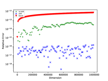
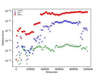
Figure 2: Relative errors in plain summation (green +) and summation with shift (blue x); and (18) (red triangle). Left panel: $x_{k}=10^{4}+\mathrm{uniform}[0,1]$. Right panel: $x_{k}=\mathrm{normal}(0,1)$.

In Figure 2, the range for the number of summands is $n=10:10^{4}:10^{6}$, and working precision is double with $u\approx 10^{-16}$. Figure 2 illustrates that, compared to plain summation, shifted summation can increase the accuracy when summands are artificially and tightly clustered at a large mean, however it can hurt the accuracy when summands are naturally clustered around zero. For the normal(0,1) summands in the right panel, the range of shifts is $.003\leq c\leq 1.2$. The expression (18) represents an upper bound accurate within a factor 10-100.

5.2 Comparison of shifted and compensated summation

We compare the errors from sequential summation with shifting (sequential version of Algorithm 1) and compensated summation (Algorithm 3).

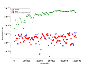
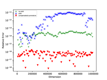
Figure 3: Relative errors in plain summation (green +), summation with shift (blue x), and compensated summation (red triangle). Left panel: $x_{k}=10^{4}+\mathrm{uniform}[0,1]$. Right panel: $x_{k}=\mathrm{normal}(0,1)$.

In Figure 3, the range for the number of summands is $n=10:10^{4}:10^{6}$, and working precision is double with $u\approx 10^{-16}$. Figure 3 illustrates that compensated summation is at least as accurate and can be much more accurate than shifted summation. in both panels, compensated summation is accurate to machine precision.

5.3 Errors and bounds for compensated summation

We compare the errors from sequential summation (sequential version of Algorithm 1) and compensated summation (Algorithm 3) with the relative version of the first order probabilistic bound in Corollary 4.13

(19) $$u\,\frac{2\|\mathbf{x}\|_{2}+|s_{n}|}{|s_{n}|}\sqrt{2\ln(2/\delta)},\qquad\mathbf{x}=\begin{bmatrix}x_{1}&\cdots&x_{n}\end{bmatrix}^{T}.$$

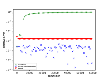
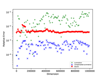
Figure 4: Relative errors in plain summation (green +), compensated (blue x), and (19) (red triangle). Left panel: $x_{k}=\mathrm{uniform}[0,1]$. Right panel: $x_{k}=\mathrm{normal}(0,1)$.

In Figure 4, the working precision is double with $u\approx 5\cdot 10^{-4}$. In the left panel the number of uniform(0,1) summands is $n=10:10^{3}:6\cdot 10^{4}$, to avoid overflow since the largest value in binary16 is about 65,504. In the right panel in contrast, the number of normal(0,1) summands is $n=10:10^{4}:10^{6}$, as summands of different signs are less likely to cause overflow.

Figure 4 illustrates that, in contrast to plain summation, compensated summation is accurate to machine precision, even for $n>u^{-1}$ in the right panel, and that (19) represents an upper bound accurate with a factor 10.

Acknowledgement

We thank Johnathan Rhyne for helpful discussions.

References

• [1] P. Blanchard, N. J. Higham, and T. Mary, A class of fast and accurate summation algorithms, SIAM J. Sci. Comput., 42 (2020), pp. A1541–A1557.
• [2] F. Chung and L. Lu, Concentration inequalities and martingale inequalities: a survey, Internet Math., 3 (2006), pp. 79–127.
• [3] M. P. Connolly, N. J. Higham, and T. Mary, Stochastic rounding and its probabilistic backward error analysis, SIAM J. Sci. Comput., 43 (2021), pp. A566–A585.
• [4] G. Constantinides, F. Dahlqvist, Z. Rakamaric, and R. Salvia, Rigorous roundoff error analysis of probabilistic floating-point computations, 2021, https://arxiv.org/abs/2105.13217.
• [5] F. Dahlqvist, R. Salvia, and G. A. Constantinides, A probabilistic approach to floating-point arithmetic, 2019, https://arxiv.org/abs/1912.00867.
• [6] J. Demmel and Y. Hida, Accurate and efficient floating point summation, SIAM J. Sci. Comput., 25 (2003/04), pp. 1214–1248.
• [7] D. Goldberg, What every computer scientist should know about floating-point arithmetic, ACM Comput. Surv., 23 (1991), pp. 5–48.
• [8] E. Hallman, A refined probabilistic error bound for sums, 2021, https://arxiv.org/abs/2104.06531.
• [9] N. J. Higham, Accuracy and stability of numerical algorithms, SIAM, Philadelphia, second ed., 2002.
• [10] N. J. Higham and T. Mary, A new approach to probabilistic rounding error analysis, SIAM J. Sci. Comput., 41 (2019), pp. A2815–A2835.
• [11] N. J. Higham and T. Mary, Sharper probabilistic backward error analysis for basic linear algebra kernels with random data, SIAM J. Sci. Comput., 42 (2020), pp. A3427–A3446.
• [12] IEEE Computer Society, IEEE Standard for Floating-Point Arithmetic, IEEE Standard 754–2008, 2019. http://ieeexplore.ieee.org/document/4610935.
• [13] I. C. F. Ipsen and H. Zhou, Probabilistic error analysis for inner products, SIAM J. Matrix Anal. Appl., 41 (2020), pp. 1726–1741.
• [14] W. Kahan, Further remarks on reducing truncation errors, Comm. ACM, 8 (1965), p. 40.
• [15] W. Kahan, Implementation of algorithms (lecture notes by W. S. Haugeland and D. Hough), Tech. Report 20, Department of Computer Science, University of California, Berkeley, CA 94720, 1973.
• [16] D. Knuth, The Art of Computer Programming, vol. II, Addison-Wesley, Reading, MA, third ed., 1998.
• [17] D. Lohar, M. Prokop, and E. Darulova, Sound probabilistic numerical error analysis, in Intern. Conf. Integrated Formal Methods, Springer, 2019, pp. 322–340.
• [18] M. Mitzenmacher and E. Upfal, Probability and computing: randomization and probabilistic techniques in algorithms and data analysis, Cambridge University Press, 2005.
• [19] A. Neumaier, Rundungsfehleranalyse einiger Verfahren zur Summation endlicher Summen, Z. Angew. Math. Mech., 54 (1974), pp. 39–51.
• [20] S. Roch, Modern discrete probability: An essential toolkit, University Lecture, (2015).